Alfvénic superradiance for a monopole magnetosphere around a Kerr black hole

Abstract

Herein, we explore superradiance for Alfvén waves (Alfvénic superradiance) in an axisymmetric rotating magnetosphere of a Kerr black hole within the force-free approximation. On the equatorial plane of the Kerr spacetime, the Alfvén wave equation is reduced to a one-dimensional Schrödinger-type equation by separating variables of the wave function and introducing a tortoise coordinate mapping the inner and outer light surfaces to $-\infty$ and $+\infty$, respectively, and we investigate a wave scattering problem for Alfvén waves. An analysis of the asymptotic solutions of the wave equation and conservation of the Wronskian provides the superradiant condition for Alfvén waves, and it is shown that the condition coincides with that for the Blandford-Znajek process. This indicates that when Alfvénic superradiance occurs, the Blandford-Znajek process also occurs in the force-free magnetosphere. Then, we evaluate the reflection rate of Alfvén waves numerically and confirm that Alfvénic superradiance is indeed possible in the Kerr spacetime. Moreover, we will discuss a resonant scattering of Alfvén waves, which is related to a “quasinormal mode” of the magnetosphere.

I Introduction

The mechanism for extracting the rotational energy from a black hole has been discussed as an energy source for high-energy astronomical phenomena such as relativistic jets in active galactic nuclei, compact objects, and gamma-ray bursts. The Blandford-Znajek (BZ) process Blandford1977 is one of the most promising candidates to describe this mechanism, which is driven by rotating black hole magnetosphere. The original BZ process Blandford1977 was discussed with focus on Kerr spacetime and force-free magnetospshere, for which the plasma inertia is ignored due to the strong electromagnetic fields. Then, they discovered that if the angular velocity of the rotating black hole $\Omega_{\text{H}}$ exceeds that of magnetic field lines $\Omega_{F}$:

$$0<\Omega_{F}<\Omega_{\text{H}},$$ (1)

the rotational energy of the black hole is transported outward in the form of the Poynting flux, which is caused by the magnetic torque acting on magnetic field lines due to the dragging effect of the rotating black hole. After the pioneering work by Blandford and Znajek in 1977 Blandford1977 , several supportive works have been conducted based on analytical and numerical computations not only for force-free manetosphere, but also for magnetohydrodynamic case, for example Toma2014 ; Toma2016 ; Jacobson2019 ; Kinoshita2018 ; Komissarov2004 ; Komissarov2005 ; Koide2006 ; McKinney2006 ; Ruiz2012 ; Koide2014 ; Koide2018 .

Superradiance Zeldovich1971 ; Zeldovich1972 ; Starobinsky1973 ; Starobinsky1974 ; Brito2015 is also an energy extraction mechanism, which is often described as a wave version of the Penrose process Penrose ; Wagh1985 ; Dadhich2012 . The condition for superradiance (superradiant condition) is given by

$$0<\dfrac{\omega}{m}<\Omega_{\text{H}},$$ (2)

where $\omega$ is the frequency of a wave and $m$ is the azimuthal quantum number. As various wave phenomena will occur in the magnetosphere, the effect of energy extraction by waves should also be considered.

Although, in general, the BZ process and superradiance are considered as different mechanisms, conditions (1) and (2) appear similar regarding the ratio $\omega/m$ as the angular velocity of a wave pattern. There must be various wave modes in a black hole magnetosphere, hence investigation of the relationship between the BZ process and superradiance is important not only for clarifying their mathematical relation, but also for understanding the essence of the BZ process. Indeed, there are several works on superradiant scattering of waves in black hole magnetospheres: superradiance for the fast magnetosonic wave Uchida1997c ; Putten1999 and energy extraction via scalar clouds as a proxy for the force-free magnetosphere Wilson-Gerow2016 , but the relationship between superradiance and the BZ process had not been clarified until our previous work Noda2020 . In our previous work Noda2020 , we investigated the relationship between the BZ process and superradiance by discussing the superradiant scattering of Alfvén waves (Alfvénic superradiance) for a force-free magnetosphere in Bañados-Teitelboim-Zanelli (BTZ) black string spacetime Jacobson2019 , and suggested that the BZ process is the zero mode of Alfvénic superradiance. The BTZ black string spacetime is asymptotically anti-de Sitter spacetime and its horizon geometry is cylinder, hence, it is not an astrophysical black hole. As black hole candidates observed so far are well-explained with Kerr black hole, it is important to check whether or not the Alfvénic superradiance is possible for a force-free magnetosphere around a Kerr black hole.

One of the differences between the magnetospheres in the BTZ string spacetime and the Kerr spacetime is the existence of the outer light surface. For the Kerr spacetime case there is an outer light surface that provides outgoing one-way boundary condition to Alfvén waves. If we solve the wave equation with the outgoing boundary condition at the outer light surface, which is similar to the computation of black hole quasinormal modes, it is possible to discuss the stability of the magnetosphere for the perturbation associated with Alfvén waves.

In this paper, we investigate the possibility of the Alfvénic superradiance in the Kerr spacetime. To achieve this, we solve the equation for force-free black hole magnetosphere in the Kerr spacetime to obtain a background magnetosphere. Then, we apply a perturbation to it and discuss the wave propagation in the background black hole magnetosphere. However, the global magnetosphere around a Kerr black hole is difficult to obtain as we need to solve the Grad-Shafranov equation Grad ; Shafranov ; Blandford1977 in the Kerr spacetime. Hence, our computation will be restricted to the electromagnetic field in the vicinity of the equatorial plane of the Kerr spacetime. Moreover, the force-free magnetosphere is assumed to be symmetric about the equatorial plane, axisymmetric, and stationary. Then, applying an appropriate perturbation to the background magnetosphere, the wave equation for Alfvén waves will be derived.

This paper is organized as follows. In section II, we review the force-free electromagnetic field and obtain the background magnetosphere around the equatorial plane of the Kerr spacetime and confirm whether the BZ process is possible for the background magnetosphere solution. In section III, the Alfvén wave equation will be derived by giving a perturbation to the background magnetosphere. Then, we rewrite the wave equation in the form of the Schrödinger-type equation to clarify the propagation and scattering problem of Alfvén waves with the effective potential. Section IV presents the discussion of Alfvénic superradiance and the derivation of the superradiant condition, and the reflection rates of Alfvén waves are evaluated with a numerical calculation. Furthermore, we discuss a resonant scattering of Alfvén waves, which is related to a “quasinormal mode” of the background magnetosphere. The conclusion is provided in section V. We use the CGS units in electromagnetism and $c=G=1$ throughout this paper.

II Force-free electromagnetic field in the Kerr spacetime

First, we briefly review the force-free approximation of the plasma-electromagnetic field system in a curved spacetime. Applying it to the Maxwell equation in the Kerr spacetime, we obtain a configuration of force-free electromagnetic field in the vicinity of the equatorial plane of the Kerr spacetime. Then, we discuss the BZ process for the background magnetosphere solution.

II.1 Force-free approximation

The basic equations are Maxwell’s equation with electric 4-current $j^{\mu}$,

$$\nabla_{\alpha}F^{\mu\alpha}=4\pi j^{\mu},\ \ \nabla_{[\mu}F_{\nu\lambda]}=0,$$ (3)

and conservation of the energy-momentum tensor,

$$\nabla_{\nu}(T^{\mu\nu}_{\text{plasma}}+T_{\text{em}}^{\mu\nu})=0,$$ (4)

where $T^{\mu\nu}_{\text{plasma}}$ is the energy momentum tensor of plasma and $T_{\text{em}}^{\mu\nu}$ is that of electromagnetic field. If the electromagnetic fields are so strong that the inertia of plasmas can be ignored, the above conservation law becomes $\nabla_{\nu}T_{\text{em}}^{\mu\nu}\simeq 0$. This is the force-free approximation. Hereafter, we simply denote $T_{\text{em}}^{\mu\nu}$ as $T^{\mu\nu}$, and it is given by

$$T_{\mu\nu}=F_{\mu\alpha}F_{\nu}^{\ \alpha}-\frac{1}{4}F_{\alpha\beta}F^{\alpha\beta}g_{\mu\nu}.$$ (5)

Using the force-free approximation, it can be shown that $\nabla_{\nu}T_{\ \mu}^{\nu}=-4\pi F_{\mu\nu}j^{\nu}\simeq 0$. Therefore, the Maxwell equation under the force-free approximation is

$$F_{\mu\nu}\nabla_{\alpha}F^{\nu\alpha}=0,\quad\nabla_{[\mu}F_{\nu\lambda]}=0.$$ (6)

For an observer of which 4-velocity is given by $u^{\mu}$, the electric field $E^{\mu}$ and the magnetic filed $B^{\mu}$ are defined as $E^{\mu}=F^{\mu\nu}u_{\nu}$ and $B^{\mu}=-{}^{*}F^{\mu\nu}u_{\nu}$, respectively. The field strength $F_{\mu\nu}$ is assumed to be magnetically dominated, as

$$F_{\mu\nu}F^{\mu\nu}=2(B^{\mu}B_{\mu}-E^{\mu}E_{\mu})>0.$$ (7)

This condition ensures the existence of a timelike observer who only sees the magnetic field. The field strength satisfying Eq. (6) can be represented with the Euler potentials $\phi_{1}$ and $\phi_{2}$ Uchida1997 ; Uchida1997a ; Uchida1997b ; Uchida1997c ; Gralla2014 as

$$F_{\mu\nu}=\partial_{\mu}\phi_{1}\partial_{\nu}\phi_{2}-\partial_{\mu}\phi_{2}\partial_{\nu}\phi_{1},$$ (8)

and the Maxwell equation with the force-free approximation yields the following nonlinear equations for the Euler potentials:

$$\partial_{\mu}\phi_{i}\partial_{\nu}\left[\sqrt{-g}\left(\partial^{\mu}\phi_{1}\partial^{\nu}\phi_{2}-\partial^{\nu}\phi_{1}\partial^{\mu}\phi_{2}\right)\right]=0,\ \ (i=1,2).$$ (9)

By solving these two equations, we obtain the Euler potentials and the field strength. In the next subsection, we present a solution around the equatorial plane of the Kerr spacetime with arbitrary values of the spin parameter.

II.2 Background force-free magnetosphere

As a background magnetosphere to investigate the propagation of Alfvén waves, we obtain a force-free magnetosphere solution with monopole-like magnetic field lines around the equatorial plane of a Kerr black hole by solving Eq. (9) with the fixed Kerr metric. First, let us introduce the Boyer-Lindquist coordinates $(t,r,\theta,\varphi)$ of the Kerr spacetime

$$g= -\left(1-\dfrac{2Mr}{\Sigma}\right)dt^{2}-\dfrac{4aMr\sin^{2}{\theta}}{\Sigma}dtd\varphi$$

$$+\dfrac{\Sigma}{\Delta}dr^{2}+\Sigma d\theta^{2}+\dfrac{A\sin^{2}{\theta}}{\Sigma}d\varphi^{2},$$ (10)

where $\Delta=r^{2}-2Mr+a^{2}$ ,  $\Sigma=r^{2}+a^{2}\cos^{2}{\theta}$ , $A=(r^{2}+a^{2})^{2}-\Delta a^{2}\sin^{2}{\theta}$, and the constants $M$ and $a$ are the mass and angular momentum per unit mass of the Kerr black hole, respectively. The outer horizon radius $r_{\text{H}}$ is given as the larger root of $\Delta=0$. The dragging of spacetime is represented by the angular velocity of the zero angular momentum observer

$$\Omega(r):=-\dfrac{g_{t\varphi}}{g_{\varphi\varphi}},$$ (11)

and the value of this function at the outer horizon is $\Omega_{\text{H}}:=a/(2Mr_{\text{H}})$. The Kerr spacetime has two Killing vectors, ${\xi}_{(t)}={\bf{\partial}}_{t}$ and ${\xi}_{(\varphi)}={\bf{\partial}}_{\varphi}$. The region where the timelike Killing vector becomes spacelike is called the ergoregion.

The solution of a monopole-type magnetic field for a force-free magnetosphere around the equatorial plane is given as

$$\phi_{1}=q\cos{\theta},\ \phi_{2}=\varphi-\Omega_{F}t+J_{B}\int\dfrac{r^{2}}{\Delta}dr,\ \text{with}\ \frac{\pi}{2}-\theta\ll 1,$$ (12)

in terms of the Euler potentials, where $q$ is the monopole charge, the angular velocity of the magnetic field line $\Omega_{F}$ is a free parameter here, and $J_{B}$ is given by the regularity condition of $F_{\mu\nu}F^{\mu\nu}$ at the horizon as

$$J_{B}=\frac{r_{\text{H}}^{2}+a^{2}}{r_{\text{H}}^{2}}(\Omega_{\text{H}}-\Omega_{F}).$$ (13)

Note that solution (12) is valid for arbitrary values of the spin parameter $a$, but it is consistent with the solution of magnetic field lines for a slowly rotating black hole obtained by Blandford1977 (see also Yang2014 ; Gralla2014 ). The derivation of solution (12) is discussed in the Appendix.

The physical meaning of the Euler potentials is as follows. The function $\phi_{1}$ is the so-called stream function, which defines a magnetic surface as $\phi_{1}=\text{const}$, and $\Omega_{F}$ is, in general, a function of $\phi_{1}$. Therefore, $\Omega_{F}$ is a constant for a fixed magnetic surface. The condition $\phi_{2}=\text{const}$ determines the shape and the time evolution of the magnetic field lines on the magnetic surface. The timelike two-dimensional surface defined by the intersection of $\phi_{1}=\text{const}$ and $\phi_{2}=\text{const}$ lying in the four-dimensional spacetime is called the field sheet Gralla2014 . Considering the above properties, we see that a constant time slice on the field sheet gives the magnetic field line on the magnetic surface at that time.

The background magnetosphere has both the inner and outer light surfaces, which are given as the condition that the corotating vector with the magnetic field line $\chi^{\mu}:=\xi_{(t)}^{\mu}+\Omega_{F}\xi^{\mu}_{(\varphi)}$ becomes null. We denote the norm of $\chi^{\mu}$ by $\Gamma$ and it is evaluated as

$$\Gamma :=g_{\mu\nu}\chi^{\mu}\chi^{\nu}=g_{tt}+2\Omega_{F}g_{t\varphi}+\Omega_{F}^{2}g_{\varphi\varphi}$$

$$=-\frac{\Omega_{F}^{2}}{r}(r_{0}-r)(r-r_{\text{in}})(r-r_{\text{out}}),\ r_{0}<0<r_{\text{in}}<r_{\text{out}}.$$ (14)

The two positive roots on the equatorial plane $\theta=\pi/2$ are obtained analytically as

$$r_{\text{in}} =2d_{1}\cos\left(\frac{1}{3}\mathrm{arccos}\left(\frac{d_{2}}{2d_{1}}\right)-\frac{2\pi}{3}\right),$$ (15)

$$r_{\text{out}} =2d_{1}\cos\left(\frac{1}{3}\mathrm{arccos}\left(\frac{d_{2}}{2d_{1}}\right)\right),$$ (16)

and these are the radii of the inner and outer light surfaces, respectively. The negative root $r_{0}$ is

$$r_{0}=2d_{1}\cos\left(\frac{1}{3}\mathrm{arccos}\left(d_{2}/(2d_{1})\right)+2\pi/3\right),$$ (17)

where

$$d_{1}=\left(\frac{1-a^{2}\Omega_{F}^{2}}{3\Omega_{F}^{2}}\right)^{1/2},\ \ d_{2}=-6M\left(\frac{1-a\Omega_{F}}{1+a\Omega_{F}}\right).$$ (18)

The inner light surface is located outside the black hole horizon: $r_{\text{H}}<r_{\text{in}}$, which is always satisfied for the present background magnetosphere. As shown in Fig. 1, $\Gamma$ is negative in the region between the light surfaces.

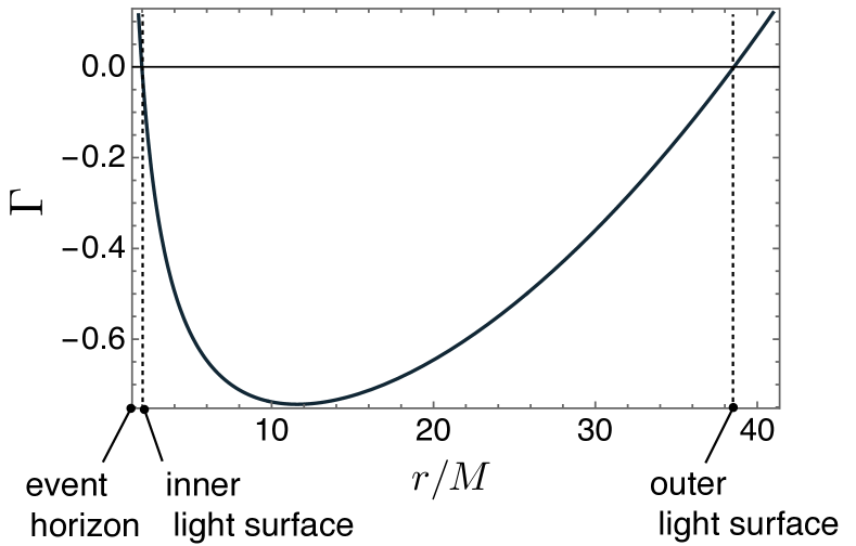
Figure 1: Plot of $\Gamma$ for $a/M=0.2$ and $M\Omega_{F}=0.027$; $\Gamma<0$ in the region between $r_{\text{in}}$ and $r_{\text{out}}$, and outside the region, $\Gamma$ becomes positive. The left end of this curve is the position of the black hole horizon.

The light surfaces are causal surfaces for propagation of Alfvén waves Gralla2014 . For all computations in the present paper, we consider Alfvén wave propagation within the range $r_{\text{in}}\leq r\leq r_{\text{out}}$ where $\chi^{\mu}$ is timelike and the velocities of corotating observers are less than the speed of light. The outer light surface forms due to the fact that the velocity of the magnetic field lines becomes faster and faster at a distant point, then finally, it exceeds the speed of light at a far point; whereas, the inner light surface is due to the effect of the gravitational redshift: Near the black hole, the speed of light is relatively slow and the velocity of the magnetic field lines becomes larger than the speed of light.

II.3 Energy and angular momentum flux

The energy and angular momentum flux vectors are defined with the timelike and spacelike Killing vectors as

$$P^{\mu}=-T^{\mu}_{\ \ \nu}\xi^{\nu}_{(t)},\quad L^{\mu}=T^{\mu}_{\ \ \nu}\xi^{\nu}_{(\varphi)}.$$ (19)

Evaluating the radial components of these vectors Blandford1977 , we obtain

$$P^{r}=-g^{rr}T_{rt}=-g^{rr}g^{\theta\theta}F_{r\theta}F_{t\theta}\simeq\Omega_{F}J_{B}\frac{q^{2}}{r^{2}}\sin^{2}{\theta},$$ (20)

$$L^{r}=g^{rr}T_{r\varphi}=g^{rr}g^{\theta\theta}F_{r\theta}F_{\varphi\theta}\simeq J_{B}\frac{q^{2}}{r^{2}}\sin^{2}{\theta},$$ (21)

where we consider $\pi/2-\theta\ll 1$. As $J_{B}\propto(\Omega_{\text{H}}-\Omega_{F})$, both the energy and angular momentum fluxes become outward only if

$$0<\Omega_{F}<\Omega_{\text{H}}.$$ (22)

This is the condition for occurrence of the BZ process, and if $\Omega_{F}=\Omega_{\text{H}}/2$, then the energy flux takes the maximum.

III Alfvén waves

In this section, we apply a perturbation to the background magnetosphere obtained in the previous section and discuss the wave propagation in the magnetosphere. There are two different wave modes in the force-free magnetosphere: the fast magnetosonic and Alfvén wave, which is a longitudinal wave mode due to the magnetic and gas pressure, and a transverse wave mode propagating along magnetic field line due to the magnetic tension. In general, these wave modes are coupled to each other, but they can be decoupled by considering the perpendicular perturbation to a magnetic surface.

III.1 Perturbation and wave modes

Let $\delta\phi_{i}$ be a perturbation to the Euler potential $\phi_{i}$ for $i=1,2$. To define the perturbation, it is useful to introduce the displacement vector Uchida1997c ; Uchida1997b in the $\theta$ direction, whose component is denoted by $\zeta^{\theta}$. Taking the inner product between the derivative of the Euler potentials of the background magnetosphere and $\zeta^{\mu}:=\delta^{\mu}_{\theta}\zeta^{\theta}$, the perturbations are obtained as

$$\delta\phi_{1}=\zeta^{\mu}\partial_{\mu}\phi_{1}=\zeta^{\theta}(t,r,\varphi)\partial_{\theta}\phi_{1},\ \ \delta\phi_{2}=\zeta^{\mu}\partial_{\mu}\phi_{2}=0$$ (23)

Note that we choose the magnetic surface on the equatorial plane of the Kerr spacetime; therefore, the first derivative of $\delta\phi_{1}$ with respect to $\theta$ becomes zero due to the definition of the perturbation and the $\theta$ dependence of the background magnetosphere solution (12). This indicates that the wave mode $\delta\phi_{1}$ does not propagate in the $\theta$ direction; specifically, the propagation of this wave mode is restricted on the magnetic surface. Moreover, its oscillation is in the perpendicular direction of the magnetic surface; therefore, $\delta\phi_{1}$ is a transverse wave mode propagating on a magnetic surface (Alfvén wave). Meanwhile, $\delta\phi_{2}$ corresponding to the fast magnetosonic wave does not appear for the present perturbation to the background magnetosphere.

From (9), the first-order perturbation equations are

$$\partial_{\mu}\delta\phi_{i}\partial_{\nu}\left[\sqrt{-g}\partial^{[\mu}\phi_{1}\partial^{\nu]}\phi_{2}\right]$$

$$\quad\quad+\partial_{\mu}\phi_{i}\partial_{\nu}\left[\sqrt{-g}\left(\partial^{[\mu}\delta\phi_{1}\partial^{\nu]}\phi_{2}\right)\right]=0.$$ (24)

For $i=1$, the second term is zero due to $\partial_{\theta}\delta\phi_{1}=0$, whereas the first term is proportional to $\pi/2-\theta\ (\ll 1)$ by expanding this quantity and becomes zero on $\theta=\pi/2$. Therefore, (24) with $i=1$ is a trivial equation. For $i=2$, we obtain

$$\partial_{\mu}\phi_{2}\partial_{\nu}\left[\sqrt{-g}\partial^{[\mu}\delta\phi_{1}\partial^{\nu]}\phi_{2}\right]=0.$$ (25)

This is the wave equation governing the propagation of Alfvén waves on the magnetic surface at $\theta=\pi/2$. A schematic of magnetic fields and the perturbation perpendicular to the magnetic surface ($\theta=\pi/2$) is displayed in Fig. 2. Note that the background magnetic field lines can have curvature in the toroidal direction, which stems from the nonzero $B^{\varphi}$ (53).

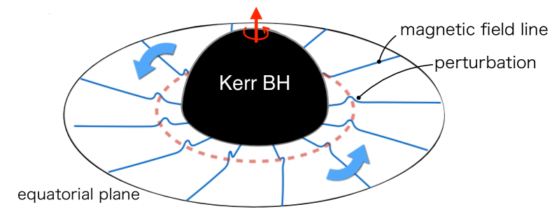
Figure 2: Schematic of the perturbation perpenducular to the magnetic surface on the equatorial plane.

III.2 Alfvén wave equation in the form of the Schrödinger equation

In this subsection, we rewrite wave equation (25) in the form of a Schrödinger-type equation by introducing a “tortoise coordinate”, which maps the inner and outer light surfaces to $-\infty$ and $+\infty$, respectively.

In terms of the Euler potentials, a magnetic field line and its time evolution is given by

$$\phi_{2}=\varphi-\Omega_{F}t+J_{B}\int\dfrac{r^{2}}{\Delta}dr=\text{const.}$$ (26)

Considering the property of Alfvén waves that propagate along a magnetic field line, we should assume the dependence of variables as

$$\delta\phi_{1}=\delta\phi_{1}\left(t,\ r,\ \varphi-\Omega_{F}t+J_{B}\int(r^{2}/\Delta)dr\right).$$ (27)

Substituting this $\delta\phi_{1}$ into (25), we obtain

$$-\dfrac{r^{2}}{\Delta}H\partial_{t}^{2}\delta\phi_{1}+\partial_{r}\left[-\Gamma\left(\partial_{r}-\dfrac{{J_{B}}r^{2}g_{\varphi\varphi}}{\Gamma\Delta}(\Omega-\Omega_{F})\partial_{t}\right)\delta\phi_{1}\right]$$

$$+\dfrac{{J_{B}}r^{2}g_{\varphi\varphi}}{\Delta}(\Omega-\Omega_{F})\partial_{t}\partial_{r}\delta\phi_{1}-|\partial\phi_{2}|^{2}\ \delta\phi_{1}=0,$$ (28)

where $|\partial\phi_{i}|^{2}:=\partial_{\mu}\phi_{i}\partial^{\mu}\phi_{i}$ and $H:=1+\Omega_{F}g_{\varphi\varphi}\partial_{r}\phi_{2}$. Note that $|\partial\phi_{2}|^{2}$ is proportional to the absolute square of the field strength as shown below:

$$\dfrac{F_{\mu\nu}F^{\mu\nu}}{2}=\left[|\partial\phi_{1}|^{2}|\partial\phi_{2}|^{2}-(\partial^{\mu}\phi_{1}\partial_{\mu}\phi_{2})^{2}\right]=\dfrac{q^{2}}{r^{2}}|\partial\phi_{2}|^{2}.$$ (29)

First, we introduce the following new coordinates to eliminate the $\partial_{t}\partial_{r}\delta\phi_{1}$ term in (28):

$$\partial_{T}=\partial_{t},\quad\partial_{X}=\partial_{r}-\dfrac{J_{B}r^{2}g_{\varphi\varphi}}{\Gamma\Delta}(\Omega-\Omega_{F})\partial_{t}.$$ (30)

The relation between the old and new coordinates is

$$r=X,\quad t=T-J_{B}\int dX\dfrac{X^{2}g_{\varphi\varphi}}{\Gamma\Delta}(\Omega-\Omega_{F}),$$ (31)

and equation (28) yields

$$\left[-\frac{X^{2}}{\Delta}H+\frac{J_{B}^{2}X^{4}g_{\varphi\varphi}^{2}}{\Gamma\Delta^{2}}(\Omega-\Omega_{F})^{2}\right]\partial_{T}^{2}\delta\phi_{1}$$

$$\quad\quad+\partial_{X}\left(-\Gamma\partial_{X}\delta\phi_{1}\right)-|\partial\phi_{2}|^{2}\delta\phi_{1}=0.$$ (32)

Then, separating the variables as $\delta\phi_{1}=e^{-i\omega T}R(X)$ and introducing the “tortoise” coordinate $x$ as $dx/dX=-\Gamma^{-1}$, we obtain the Schrödinger-type equation

$$\dfrac{d^{2}R}{dx^{2}}-V_{\text{eff}}R=0,$$ (33)

$$V_{\text{eff}}=-\Gamma|\partial\phi_{2}|^{2}+\dfrac{\omega^{2}X^{2}}{\Delta}\left[H\Gamma-\frac{J_{B}^{2}X^{2}g_{\varphi\varphi}^{2}}{\Delta}(\Omega-\Omega_{F})^{2}\right].$$ (34)

In the tortoise coordinate, the locations of the inner and outer light surfaces becomes $x=-\infty$ and $x=+\infty$, respectively. The effective potentials for several frequencies are plotted in Fig. 3.

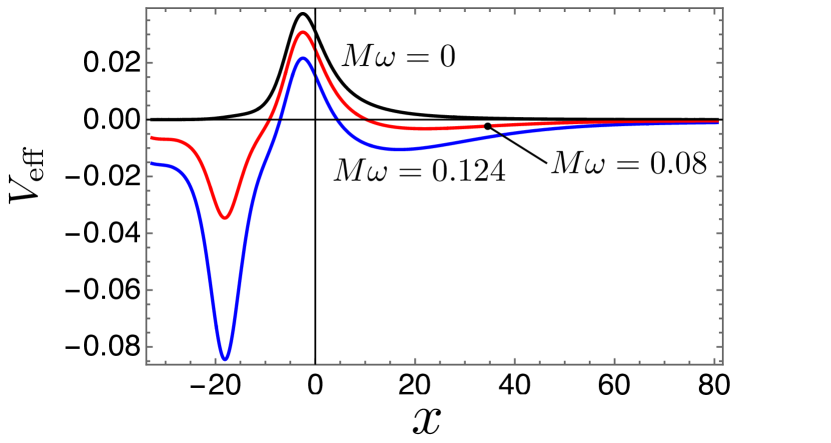
Figure 3: Effective potentials $V_{\text{eff}}$ for Alfvén waves propagating on the magnetic surface in the vicinity of the equatorial plane for $a/M=0.2$, $M\Omega_{F}=0.041$ with $M\omega=0,0.08,0.124$. The parameter set $(M\Omega_{F},M\omega)=(0.041,0.124)$ gives a deep bottom, and a resonance can be seen as displayed in Fig. 6.

Note that the $x$-dependence of the terms with $\omega$ in (34) is very small, as seen from Fig. 3. Therefore, properties of the effective potential, such as the existence and the position of the peak, are determined by the first term, which reflects the effect of the gravitational redshift and the angular velocity of magnetic field lines in $\Gamma$ as well as the square of the field strength.

IV Alfvénic superradiance and resonant scattering

In this section, we discuss the wave scattering problem of Alfvén waves by solving Schrödinger-type equation (33) for the corotating coordinates $(T,x)$. For Alfvén waves to be scattered by the effective potential efficiently, we focus only on the relatively low frequency cases: $M\omega=0.050$ - $0.250$. From the coefficients of the asymptotic ingoing and outgoing solutions, we define the reflection rate of the Alfvén waves, then obtain the condition for Alfvénic superradiance.

IV.1 Reflection rate of Alfvén waves and the condition for Alfvénic superradiance

To evaluate the asymptotic form of the wave function $R$ in Eq. (33), first, we examine the asymptotic form of the effective potential. Then, the definition of ingoing and outgoing modes in this scattering problem is discussed. As $\Gamma\simeq 0$ in the vicinity of the two light surfaces, the asymptotic form of the effective potential is

$$V_{\text{eff}}^{\text{asymp}}\simeq-\dfrac{\omega^{2}J_{B}^{2}X^{4}g_{\varphi\varphi}^{2}}{\Delta^{2}}(\Omega-\Omega_{F})^{2}\ <0.$$ (35)

Therefore, the asymptotic solution of Eq. (33) is written in the following form:

$$R \propto\exp{\left[\pm i\int dx\sqrt{-V_{\text{eff}}^{\text{asymp}}}\right]}$$

$$=\exp{\left[\pm i\omega\int dx\dfrac{X^{2}g_{\varphi\varphi}}{\Delta}|J_{B}|(\Omega_{F}-\Omega)\ \right]},$$ (36)

where $\omega,X^{2},g_{\varphi\varphi}$, and $\Delta$ are positive definite quantities, whereas the sign of $\Omega-\Omega_{F}$ can be changed depending on the value of $\Omega_{F}$ and the location $r$. At a point far from the black hole where the dragging effect of the spacetime is almost zero: $\Omega\sim 0$ and the sign of the integrand in (36) is positive. Therefore, the positive (negative) sign in (36) indicates the outgoing (ingoing) wave there. We use this asymptotic behavior of the phase of the wave function to define the in and outgoing modes.

As the inner light surface is the causal boundary for Alfvén waves Gralla2014 , we require the purely ingoing boundary condition at the inner light surface. The asymptotic solutions of Eq. (33) with the ingoing boundary condition at the light surfaces are

$$R=\begin{cases}{\displaystyle\exp{\left[-i\omega\int\frac{dx}{\Delta}X^{2}g_{\varphi\varphi}|J_{B}|(\Omega_{F}-\Omega)\right]}}\quad\quad\quad\quad\quad\quad\quad\quad\quad\quad\quad\quad\quad\quad\quad\quad\quad\quad\quad\ \text{for}\quad x\rightarrow-\infty,\\ {\displaystyle A_{\text{in}}{\displaystyle\exp{\left[-i\omega\int\frac{dx}{\Delta}X^{2}g_{\varphi\varphi}|J_{B}|(\Omega_{F}-\Omega)\right]}}+A_{\text{out}}{\displaystyle\exp{\left[i\omega\int\frac{dx}{\Delta}X^{2}g_{\varphi\varphi}|J_{B}|(\Omega_{F}-\Omega)\right]}}}\ \text{for}\quad x\rightarrow+\infty.\end{cases}$$ (37)

The ingoing wave around the inner light surface becomes outward when the spacetime dragging effect is so large that the sign of the integrand get flipped. From the conservation of the Wronskian, we obtain the reflection rate of the wave as

$$\left|\frac{A_{\text{out}}}{A_{\text{in}}}\right|^{2}=1-\dfrac{f_{\text{in}}}{f_{\text{out}}}\dfrac{(\Omega_{F}-\Omega|_{r_{\text{in}}})}{(\Omega_{F}-\Omega|_{r_{\text{out}}})}\dfrac{1}{|A_{\text{in}}|^{2}}\ ,$$ (38)

where $f_{\text{in/out}}=(X^{2}g_{\varphi\varphi}/\Delta)|_{r_{\text{in/out}}}$. From Eq. (38), one sees that the reflection rate $|A_{\text{out}}/A_{\text{in}}|^{2}$ exceeds unity and the reflected Alfvén wave will be amplified through the scattering by the effective potential (Alfvénic superradiance) if the angular velocity of the magnetic field line satisfies

$$\Omega|_{r_{\text{out}}}<\Omega_{F}<\ \Omega|_{r_{\text{in}}}.$$ (39)

Note that the functions $\Omega|_{r_{\text{in/out}}}$ depend on $\Omega_{F}$, hence we need to solve the inequality for $\Omega_{F}$ to evaluate it. As the functions $\Omega|_{r_{\text{in/out}}}$ are too algebraically complex to solve, instead of that, we plot those functions of $\Omega_{F}$ in Fig. 4. The superradiant condition (39) holds only in the region II where

$$0<\Omega_{F}<\Omega_{\text{H}},$$ (40)

in Fig. 4. Therefore, the superradiant condition (39) is exactly the same as the condition for the BZ process (22).

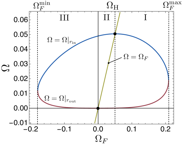
Figure 4: Relationship among functions $\Omega=\Omega|_{r_{\text{in}}}(\Omega_{F}),\Omega=\Omega|_{r_{\text{out}}}(\Omega_{F})$, and $\Omega=\Omega_{F}$ for a fixed spin parameter $a/M=0.2$. The black dots correspond to the solutions of $\Omega|_{r_{\text{in}}}(\Omega_{F})=\Omega_{F}$ and $\Omega|_{r_{\text{out}}}(\Omega_{F})=\Omega_{F}$, which are $\Omega_{F}=\Omega_{\text{H}}$ and $\Omega_{F}=0$, respectively. The minimum and maximum of $M\Omega_{F}$ for the existence of two light surfaces are denoted by $\Omega_{F}^{\text{min}}$ and $\Omega_{F}^{\text{max}}$, respectively.

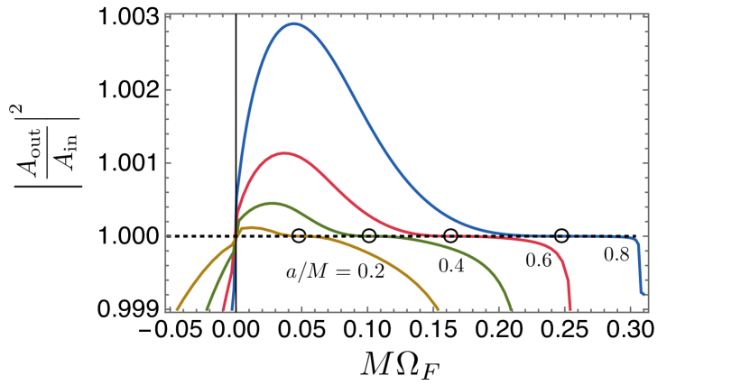
Figure 5: Reflection rate for the $M\omega=0.02$ case with several spin parameters. The threshold for $M\Omega_{F}$, which is marked as $\circ$, is given by the angular velocity of the black hole horizon, as we expected from Eq. (39), Eq. (22), and Fig. 4. The values are $M\Omega_{\text{H}}=0.0505,0.104,0.167,0.250$ for $a/M=0.2,0.4,0.6,0.8$, respectively.

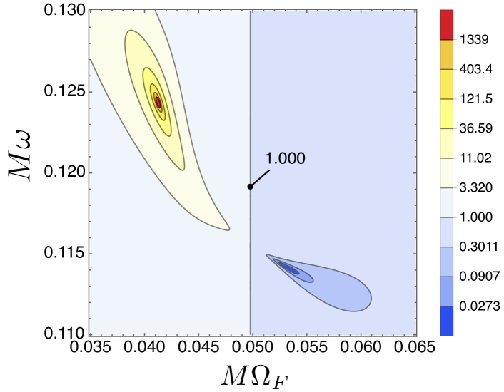
Figure 6: Contour plot of $|A_{\text{out}}/A_{\text{in}}|^{2}$ on $\Omega_{F}$-$\omega$ plane for the $a/M=0.2$ case. The vertical line labeled as $1.000$ is the contour of $|A_{\text{out}}/A_{\text{in}}|^{2}=1$.

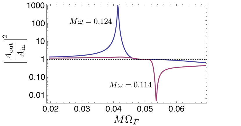
Figure 7: Reflection rates for the frequencies giving the resonant scattering and absorption in the $a/M=0.2$ case.

For $M\Omega_{F}$ in regions I–III, we evaluate the reflection rate by solving wave equation (33) numerically. The results for various spin parameters of the Kerr spacetime $a/M$ with fixed $M\omega$ are shown in Fig. 5. Indeed, the reflection rate exceeds unity for $M\Omega_{F}$ satisfying superradiant condition (39) or equivalently (22).

In Fig. 6, we present the contour plot of the reflection rate on the $\Omega_{F}$-$\omega$ plane for $a/M=0.2$. The contours of $|A_{\text{out}}/A_{\text{in}}|^{2}=1$ correspond to $M\Omega_{F}=0$ and $M\Omega_{F}=M\Omega_{\text{H}}$. Alfvénic superradiance occurs in the region between these two lines. There is a peak associated with $A_{\text{in}}\sim 0$ at $(M\Omega_{F},M\omega)=(0.0412,0.124)$. As this situation is similar to the quasinormal modes of black hole perturbation, which come from the boundary condition $A_{\text{in}}=0$ with complex frequency, we search the frequency in the complex plane of $\omega$ with the fixed angular velocity of the magnetic field line $M\Omega_{F}=0.0412$. As a result, we realized a frequency giving $A_{\text{in}}=0$ at $M\omega=0.1240-0.0002\ i$. Therefore, the peak in Fig. 6 reflects a resonant scattering corresponding to a “quasinormal mode” of the magnetosphere for Alfvénic perturbation. As the imaginary part of those frequencies are negative, the present magnetosphere is stable for the perturbation with Alfvénic superradiance. Moreover, there is a bottom at $(M\Omega_{F},M\omega)=(0.054,0.114)$. The presence of the bottom comes from $A_{\text{out}}=0$, which corresponds to a resonant absorption of Alfvén waves. For those two cases with resonant scattering, the reflection rates are plotted in Fig. 7.

V Discussion and Concluding Remarks

In this paper, based on the force-free approximation, we discussed Alfvénic superradiance in the Kerr spacetime to investigate the difference from our previous work for the BTZ black string spacetime Noda2020 . The structure of the background magnetic field lines considered here is a monopole-like in the poloidal plane, and the inner and outer light surfaces exist. We investigated the propagation of Alfvén waves by applying a perturbation perpendicular to the magnetic surface in the vicinity of the equatorial plane of the Kerr spacetime.

Introducing the tortoise coordinate $x$, the wave equation for Alfvén waves can be written in the form of the Schrödinger-type equation. To investigate the reflection rate, we defined the in and outgoing waves at asymptotic regions near the inner and outer light surfaces. Then, considering the conservation of the Wronskian, we derived the superradiant condition for Alfvén waves, which is exactly the same as that for the BZ process. Due to the existence of the outer light surface, the superradiant condition in the Kerr spacetime appears to be slightly modified from the condition derived in Noda2020 ; however, in Fig. 4, both are shown to be the same as the condition for the BZ process after all.

The result of this study demonstrates that Alfvénic superradiance, which was discussed only for the magnetosphere around a BTZ black string Noda2020 , is possible for the Kerr spacetime case as well. Therefore, it would be important for the extraction process of the rotational energy of astrophysical black holes regarding relativistic jets and/or high-energy radiations in active galactic nuclei or gamma ray bursts. In particular, the resonant scattering is determined by not only the frequency of Alfvén waves, but also the parameter of the mangetosphere such as $\Omega_{F}$, and the structure of magnetosphere, specifically that it provides the shape of the effective potential. If we observe this resonant scattering as a burst-like emission of electromagnetic waves, information on the structure of the magnetosphere and the black hole spacetime would be derived.

The dynamical situation and higher order of the perturbation are also important, as discussed in the recent work Koide2021 . A higher order of perturbation can generate a richer phenomenon, as suggested in Koide2021 : The second order perturbation to $\phi_{2}$ obeys the Klein-Gordon equation with a source term determined by $\delta\phi_{1}$. Specifically, the linear Alfvén waves can evoke the second order fast magnetosonic wave. Regarding this, a nonlinear effect that results in the conversion of Alfvén waves to fast magnetosonic waves in rotating magnetospheres around neutron stars has been discussed in Yuan2021 .

We restricted the discussion herein to a stationary magnetosphere filled with a strong magnetic field, for which the force-free approximation is valid. To grasp what really happens around astrophysical black holes, it is necessary to consider the plasma effects and the environment around a black hole such as an accretion disk, and to discuss how the rotational energy extracted by Alfvén waves can be transported and converted into the kinetic energy of plasmas and how they contribute to the relativistic jets. We leave these tasks for our next papers.

Appendix A Derivation of the background magnetosphere near the equatorial plane

Here, we demonstrate the derivation of background magnetosphere solution (12) by solving the following basic equation of the force-free electrodynamics:

$$\partial_{\mu}\phi_{i}\partial_{\nu}\left[\sqrt{-g}\left(\partial^{\mu}\phi_{1}\partial^{\nu}\phi_{2}-\partial^{\nu}\phi_{1}\partial^{\mu}\phi_{2}\right)\right]=0.\ \ \ \ (i=1,2)$$ (41)

In general, the Euler potentials for stationary and axisymmetric magnetosphere can be written as

$$\phi_{1}=\Psi(r,\theta),\ \phi_{2}=\varphi-\Omega_{F}(\Psi)t+\Phi(r,\theta).$$ (42)

This was discussed by Uchida Uchida1997a with Killing vectors. Here, to obtain a force-free magnetosphere in the vicinity of the equatorial plane, we assume that functions $\Psi$ and $\Phi$ in the Euler potentials depend on the variables as

$$\phi_{1}=\Psi(\theta),\ \phi_{2}=\varphi-\Omega_{F}t+\Phi(r),$$ (43)

where $\Omega_{F}$ is a constant corresponding to the angular velocity of magnetic field lines. Substituting this ansatz into Eq. (41) and expanding it up to the first order of the small angle measured from the equatorial plane, we obtain:

$$\epsilon=\frac{\pi}{2}-\theta.$$ (44)

First, for $i=1$, (41) yields

$$0 =\partial_{\theta}\Psi\ \partial_{\nu}\left(\sin\theta\ \partial_{\theta}\Psi\partial^{\nu}\phi_{2}\right)$$

$$=\sin\theta(\partial_{\theta}\Psi)^{2}\ \partial_{\nu}\left(\partial^{\nu}\phi_{2}\right).$$ (45)

Assuming $\sin\theta(\partial\Psi)^{2}\neq 0$, we obtain

$$\partial_{r}\left(\dfrac{\Delta}{\Sigma}\partial_{r}\Phi\right)=0.$$ (46)

Considering the fact $\Sigma=r^{2}+a^{2}\cos^{2}{\theta}=r^{2}+{\cal{O}}(\epsilon^{2})$, the above equation becomes the differential equation only for $r$. Then, the solution is

$$\Phi(r)=J_{B}\int\dfrac{r^{2}}{\Delta}\ dr.$$ (47)

The constant $J_{B}$ stems from $\Delta/r^{2}\partial_{r}\Phi=\text{const}:=J_{B}$ and is determined by the regularity of $F_{\mu\nu}F^{\mu\nu}$ at the black hole horizon. For $i=2$, (41) gives

$$0 =\partial_{\nu}\phi_{2}\partial_{\theta}\left(\sqrt{-g}\partial^{\theta}\phi_{1}\partial^{\nu}\phi_{2}\right)$$

$$=|\partial\phi_{2}|^{2}\partial_{\theta}\left(\sin\theta\ \partial_{\theta}\Psi\right)+\sin\theta\ \partial_{\theta}\Psi\ \partial_{\theta}|\partial\phi_{2}|^{2},$$ (48)

where $|\partial\phi_{2}|^{2}:=\partial_{\nu}\phi_{2}\partial^{\nu}\phi_{2}$, which is expanded as

$$|\partial\phi_{2}|^{2}=(\text{function of}\ r)+{\cal{O}}(\epsilon^{2}).$$ (49)

The derivative of $|\partial\phi_{2}|^{2}$ with respect to $\theta$ is proportional to $\cos\theta$, hence it is ignored in the present approximation. Therefore, Eq. (48) finally yields

$$\partial_{\theta}\left(\sin\theta\Psi(\theta)\right)=0,$$ (50)

for which, the solution is

$$\Psi(\theta)=q\cos\theta,$$ (51)

in the vicinity of the equatorial plane. Here, $q$ represents the monopole charge. Thus, the background force-free magnetosphere solution is obtained as (12).

To investigate the structure of the magnetic field lines, we compute the electro and magnetic fields on the equatorial plane measured by a Killing observer whose four velocity is $u^{\nu}=(1,0,0,0)$. The nonzero components of the electric and magnetic fields are

$$E^{\theta}=\frac{q\Omega_{F}}{r^{2}},\ \ B^{r}=\dfrac{q}{r^{2}}(g_{tt}+\Omega_{F}g_{t\varphi}),$$ (52)

$$B^{\varphi}=-\dfrac{qJ_{B}}{r^{2}}g_{tt}\ \ B^{t}=\dfrac{qJ_{B}}{\Delta}g_{t\varphi}.$$ (53)

Note that this background solution corresponds to a monopole-like magnetosphere in the vicinity of the equatorial plane of the Kerr spacetime.

References

- (1) R. D. Blandford and R. L. Znajek, Electromagnetic extraction of energy from Kerr black holes, Mon. Not. R. Astron. Soc. 179, 433 (1977).
- (2) K. Toma and F. Takahara, Electromotive force in the Blandford-Znajek process, Mon. Not. R. Astron. Soc. 442, 2855 (2014).
- (3) K. Toma and F. Takahara, Causal production of the electromagnetic energy flux and role of the negative energies in the Blandford-Znajek process, Prog. Theor. Exp. Phys. 3E01 (2016).
- (4) T. Jacobson and M. J. Rodriguez, Blandford-Znajek process in vacuo and its holographic dual, Phys. Rev. D 99, 124013 (2019).
- (5) S. Kinoshita and T. Igata, The essence of the Blandford-Znajek process, Prog. Theor. Exp. Phys., 3E02 (2018).
- (6) S. S. Komissarov, Electrodynamics of black hole magnetospheres, Mon. Not. R. Astron. Soc. 350, 427 (2004).
- (7) S. S. Komissarov, Observations of the Blandford-Znajek process and the magnetohydrodynamic Penrose process in computer simulations of black hole magnetospheres, Mon. Not. R. Astron. Soc. 359, 801 (2005).
- (8) S. Koide, T. Kudoh, and K. Shibata, Jet formation driven by the expansion of magnetic bridges between the ergosphere and the disk around a rapidly rotating black hole, Am. Phys. Soc. 74, 044005 (2006).
- (9) J. C. McKinney, General relativistic magnetohydrodynamic simulations of the jet formation and large-scale propagation from black hole accretion systems, Mon. Not. R. Astron. Soc. 368, 1561 (2006).
- (10) S. S. Komissarov, The role of the ergosphere in the Blandford-Znajek process, Mon. Not. R. Astron. Soc. 423, 1300 (2012).
- (11) S. Koide and T. Baba, Causal extraction of black hole rotational energy by various kinds of electromagnetic fields, Astrophys. J. 2, 88 (2014).
- (12) S. Koide and T. Imamura, Dynamic process of spontaneous energy radiation from spinning black holes through force-free magnetic field, Astrophys. J. 864, 173 (2018).
- (13) Y. B. Zel’dovich, The generation of Waves by a rotating body, Zh. Eksp. Teor. Fiz. Pis’ma Red. 14, 270, (1971). Sov. Phys. JETP Lett. 14, 180 (1971).
- (14) Y. B. Zel’dovich, Amplification of cylindrical electromagnetic waves reflected from a rotating body, Sov. Phys. JETP 35, 1085 (1972).
- (15) A.A. Starobinsky, Amplification of waves from a rotating black hole, Zh. Eksp. Teor. Phyz. 64, 48 (1973). [Sov. Phys. - JETP 37, 28 (1973).]
- (16) A.A. Starobinsky and S.M. Churilov, Amplification of electromagnetic and gravitational waves scattered by a rotating “black hole”, Zh. Eksp. Teor. Phyz. 65, 3 (1973). [Sov. Phys. - JETP 38, 1 (1974).]
- (17) R. Brito, V. Cardoso, and P. Pani, Superradiance, Lect. Notes Phys. 906, 1 (2015).
- (18) R. Penrose, Gravitational collapse: The role of general relativity, Riv. Nuovo Cimento. 1, 252 (1969).
- (19) S. M. Wagh, S. V. Dhurandhar, and N. Dadhich, Revival of the Penrose process for astrophysical applications, Astrophys. J. 290, 12 (1985).
- (20) N. Dadhich, Magnetic Penrose Process and Blanford-Zanejk mechanism: A clarification, arXiv:1210.1041 [gr-qc]
- (21) T. Uchida, Linear perturbations in force-free black hole magnetospheres II . Wave propagation, Mon. Not. R. Astron. Soc. 291, 125 (1997).
- (22) M. H. P. M. van Putten, Superradiance in a torus magnetosphere around a black hole, Science 284, 115 (1999).
- (23) J. Wilson-Gerow, and A. Ritz, Black hole energy extraction via a stationary scalar analog of the Blandford-Znajek mechanism, Phys. Rev. D 93, 044043 (2016).
- (24) S. Noda, Y. Nambu, T. Tsukamoto, and M. Takahashi, Blandford-Znajek process as Alfvénic superradiance, Phys. Rev. D 101, 023003 (2020).
- (25) H. Grad and H. Rubin, Hydromagnetic Equilibria and Force-Free Fields, Proceedings of the Second United Nations Conference on the Peaceful Uses of Atomic Energy (Geneva) 31 190 (1958).
- (26) V. Shafranov, Plasma Equilibrium in a Magnetic Field, Reviews of Plasma Physics 2 103 (1966).
- (27) T. Uchida, Theory of force-free electromagnetic fields. I. General theory, Phys. Rev. E 56, 2181 (1997).
- (28) T. Uchida, Theory of force-free electromagnetic fields. II. Configuration with symmetry, Phys. Rev. E 56, 2198 (1997).
- (29) T. Uchida, Linear perturbations in force-free black hole magnetospheres - I. General theory, Mon. Not. R. Astron. Soc. 286, 931 (1997).
- (30) S. E. Gralla and T. Jacobson, Spacetime approach to force-free magnetospheres, Mon. Not. R. Astron. Soc. 445, 2500 (2014).
- (31) H. Yang and F. Zhang, Stability of force-free magnetospheres, Phys. Rev. D 90, 104022 (2014).
- (32) S. Koide, S. Noda, M. Takahashi, and Y. Nambu, One-dimensional force-free numerical simulations of Alfvén waves around a spinning black string, arXiv:2109.05703 [astro-ph]
- (33) Y. Yuan, Y. Levin, A. Bransgrove, and A. Philippov, Alfvén Wave Mode Conversion in Pulsar Magnetospheres, Astrophys. J. 908, 176 (2021).