Supercurrent Diode Effect, Spin Torques, and Robust Zero-Energy Peak in Planar Half-Metallic Trilayers

Abstract

We consider a Josephson junction with F₁F₂F₃ ferromagnetic trilayers in the ballistic regime, where the magnetization in each ferromagnet ${\rm F}_{i}~{}(i=1,2,3)$, can have arbitrary orientations and magnetization strengths. The trilayers are sandwiched between two $s$-wave superconductors with a macroscopic phase difference $\Delta\varphi$. With our generalised theoretical and numerical techniques, we are able to study the planar spatial profiles and $\Delta\varphi$-dependencies of the charge supercurrents, spin supercurrents, spin torques, and density of states for complex systems that are finite in two dimensions. A broad range of magnetization strengths of the central $\rm F_{2}$ layer are considered, from an unpolarized normal metal (N) to a half-metallic phase, supporting only one spin species. Our results reveal that when the magnetization configuration in F₁F₂F₃ has three orthogonal components, a supercurrent can flow at $\Delta\varphi=0$, and a strong second harmonic in the current-phase relation appears. Remarkably, upon increasing the magnetization strength in the central ferromagnet layer up to the half-metallic limit, the self-biased current and second harmonic component become dramatically enhanced, and the critical supercurrent reaches its maximum value. The higher harmonics in the current-phase relations can be controlled by the relative magnetization orientations, with negligible current damping compared to the corresponding F₁N F₃ counterparts. Additionally, for a broad range of exchange field strengths in the central ferromagnet ${\rm F}_{2}$, the ground state of the system can be tuned to an arbitrary phase difference $\varphi_{0}$, e.g., by rotating the magnetization in the outer ferromagnet $\rm F_{3}$. For intermediate exchange field strengths in ${\rm F}_{2}$, a $\varphi_{0}$ state can arise that creates a superconducting diode effect, whereby $\Delta\varphi$ can be tuned to create a one-way dissipationless current flow. The spatial maps of the spin currents and effective magnetic moments reveal a long-ranged spin torque in the half-metallic phase. Moreover, the density of states studies demonstrate the emergence of zero energy peaks for the mutually orthogonal magnetization configurations, which is strongest in the half-metallic phase. Our results suggest that this simple trilayer Josephson junction can be an excellent candidate for producing experimentally accessible signatures for long-ranged self-biased supercurrents, and supercurrent diode-effects.

I Introduction

The competition of ferromagnetic and superconducting orders in hybrid junction systems has been the focus of extensive research over the past decades. When constructing devices that consist of superconductor (S) and ferromagnet (F) elements, the F₁SF₂ and SF₁F₂ spin valves are some of the simplest configurations with externally controlled system properties. Such platforms have been extensively studied experimentally and theoretically [1, 3, 5, 6, 7, 8, 9, 10, 2, 12, 13, 11, 14, 4, 15, 16, 17, 18]. In addition to the geometrical properties like the layer thicknesses, the relative magnetization misalignment in these systems plays a pivotal role in determining the end functionality of these systems. To effectively control the magnetization misalignment, one needs to judiciously choose materials with the proper magnetization strengths so that an external magnetic field can rotate the magnetization in one of the F regions while the other one remains essentially intact [9, 4, 10].

The presence of magnetization inhomogeneity and spin-orbit coupling can result in long-ranged spin-triplet superconducting correlations [5]. These long-ranged correlations are predicted to leave their imprint on various measurable quantities, including the critical supercurrent [21, 11, 24, 19, 20, 23, 22] and zero-energy density of states [25, 26, 27, 28, 29, 30]. An unambiguous observation of the triplet correlations in the DOS still has yet to be found. However, the critical supercurrent has revealed compelling evidence of triplet correlations by employing a relatively thick half-metallic (H) layer of $\rm CrO_{2}$ (0.3-1 $\upmu$m) in a NbTiN-$\rm CrO_{2}$-NbTiN Josephson configuration [22]. Additionally, a magnetization-orientation dependent supercurrent response on the order of $40~{}\upmu$A was observed, hinting at a controlled long-ranged spin supercurrent. When the ferromagnet is in a half-metallic phase, the very large magnetization strength (on the order of Fermi energy) permits only one spin to exist [31]. In recent years, heterostructures consisting of H layers have attracted much attention and caused further advances in this research field [36, 37, 32, 33, 34, 35]. The H layer has shown that both theoretically and experimentally, it can provide an enhancement to the critical temperature, and induce a strong nonuniform response to the magnetization misalignment in multilayer structures [36, 37, 38, 29, 30]. In an experiment involving a MoGe-Ni-Cu-CrO₂ spin valve, the superconducting critical temperature $T_{c}$ showed variations on the order of $\Delta T_{c}\!\sim\!800$mK with variations in the magnetization misalignment angle, in excellent agreement with theoretical results [29, 30]. A $\rm La_{0.6}Ca_{0.4}MnO_{3}$ half-metal counterpart, consisting of a LCMO-Au-Py-Cu-Nb stack, showed $\Delta T_{c}\!\sim\!150$mK, which is a slight improvement over $\Delta T_{c}\!\sim\!50$mK found in systems that use weaker ferromagnetic counterparts [13]. The former experiment [37] employed a large out-of-plane external magnetic field of $H\sim 2$T whereas the latter experiment [36] used a relatively low in-plane magnetic field of $H\!\sim\!3.3$mT that improves device reliability.

The Josephson effect is traditionally understood to be the supercurrent that is generated when there is a difference between the macroscopic phases of two S banks that are separated by an intrinsically non-superconducting region. Once a supercurrent is established, its flow depends on the geometrical parameters, phase differences, and material properties of the system. In a conventional ferromagnetic Josephson junction, the ground state energy can switch between specific superconducting phase differences, typically $\Delta\varphi=0$ and $\pi$, due to the dominant first harmonic in the current-phase relation: $\sin\Delta\varphi$ [60, 4]. Additionally, close to any $0$-$\pi$ crossover, higher harmonics, i.e., $\sin 2\Delta\varphi$, $\sin 3\Delta\varphi\ldots$, can appear. The higher harmonics can cause a continuous transition from $0$ state to the $\pi$ state [39, 40]. A finite supercurrent at zero phase difference, $\Delta\varphi=0$, can also arise, and the Josephson ground-state can be characterized by a superconducting phase difference $\varphi_{0}$. There are two $\varphi_{0}$ ground states located symmetrically around $\Delta\varphi=0$ associated with this continuous transition, and can have no spontaneous current.[39, 40] Note that a $\varphi_{0}$ junction introduces excellent opportunities to introduce quantum computer bits other than $0$ and $\pi$. Another mechanism to induce a $\varphi_{0}$ ground state is a proper combination of magnetization direction and spin-orbit coupling.[62, 61, 63, 41, 42, 43, 44, 45, 46, 47, 48, 49, 50, 39, 51, 52, 53, 64, 65, 66, 67, 68] In this case, the $\varphi_{0}$ is associated with a self-biased spontaneous supercurrent and located on one side of $\Delta\varphi=0$, depending on the direction of magnetization and spin-orbit coupling.[39] This mechanism is found to appear in a wide range of materials platform in the presence and absence of nonmagnetic impurities, such as topological insulators [41, 42, 43, 44], Weyl semimetals [45, 46, 47], black phosphorus [48, 49], linear Rashba-Dressehalus spin-orbit coupled platforms for revealing a persistent spin helix [50], and cubic Rashba-Dressehalus systems [39]. Another configuration that hosts a self-biased supercurrent and has received far less attention is a spin-polarized Josephson junction with a simple arrangement of three ferromagnets having their magnetization orientations each orthogonal to one another [51, 52, 53].

The supercurrent $J(\Delta\varphi)$ in spin-polarized Josephson junctions can be controlled by a variety of mechanisms, including through magnetization rotations, and incorporating different types of magnets with mismatched exchange-field strengths. For trilayer ferromagnetic Josephson junctions, including those that contain half-metallic layers, and where only two of the exchange field vectors are orthogonal, the supercurrent direction can be altered by changing the relative magnetization orientation [24, 74]. If the ground state of the Josephson junction is at $\varphi_{0}=0$, the supercurrent generally obeys $|J(+\Delta\varphi)|=|J(-\Delta\varphi)|$. In some special cases, a superconducting diode effect can arise, whereby $|J(+\Delta\varphi+\varphi_{0})|\neq|J(-\Delta\varphi+\varphi_{0})|$. When this occurs, changing the direction of the superconducting phase gradient, i.e., $\Delta\varphi\rightarrow-\Delta\varphi$, the amplitude for the supercurrent is no longer invariant. We find that remarkably, for the simple trilayer ferromagnet SF₁F₂F₃S structure shown in Fig. 1, where the exchange field vectors in the ferromagnet layers are orthogonal to one another, a diode effect emerges for the supercurrent at intermediate exchange field strengths of the central ferromagnet.

The main aim of this paper is therefore to present an extensive investigation of the influence of the many relevant physical parameters on the spin and charge transport in SF₁F₂F₃S ferromagnetic Josephson configurations. We will use for these purposes a tailor made numerical method that allows for the exact solutions of the relevant microscopic equations for Josephson strictures that are finite in two-dimensions. To systematically explore a broad range of systems and determine experimentally relevant parameter sets resulting in a tunable $\varphi_{0}$ state and supercurrent flow, the magnetization in one of the ferromagnet layers will have its magnitude continuously increased up to the half-metallic phase, and several key orientations will be investigated. To further understand the quantum size-effects inherent to structures constrained in two-dimensions, a variety of structure lengths and widths will be studied (see Fig. 1). Moreover, the often extreme ranges in energy scales for these types of systems require a microscopic theory without the approximations inherent to quasiclassical approaches. To properly simulate these experimentally relevant systems, we have therefore generalized the numerical Bogoliubov de Gennes (BdG) approach to planar geometries where the system is confined in two dimensions and infinite along the third dimension [59, 57, 29, 30, 36]. The microscopic method used here accounts for the significant band curvature near the Fermi energy arising from the strong spin-splitting effects of the half-metallic layers. This numerical approach has also found excellent agreement with results that rely on asymptotic approximations, such as the Andreev approximation [59], ab initio calculations [58], and supports the half-metallic phase where the magnetization strength is as large as the Fermi level [29, 30, 36]. This latter phase is inaccessible to approximate methods, such as the quasiclassical approach, which considers the Fermi level to be the largest energy in the system [56, 54, 55, 38, 21, 20].

We shall explore the whole of the parameter range that accounts for the effects that finite sample size, relative magnetizations (magnitude and orientation), and macroscopic phase differences have on the singlet and triplet pair amplitudes, magnetic moments, and local density of states (DOS). We will identify the ground state with phase difference $\varphi_{0}$ that is tunable by changes to the magnetization orientation of the outer ferromagnet. For intermediate exchange field strengths in the central $F$ layer, we find the emergence of a $\varphi_{0}$ state with a one-way supercurrent flow, i.e., a superconducting diode effect. Further increases of the magnetization strength in the $\rm F_{2}$ layer enhances the supercurrent so that the critical supercurrent reaches a maximum at the half-metallic phase. This magnetization increase induces $0$-$\pi$ transitions and controls the induction of higher harmonics in the current-phase-relation. When the magnetization in the F layers has mutually orthogonal components, a spontaneous supercurrent flows through the system, which is strongest when the $\rm F_{2}$ layer hosts a half-metal. The spatial maps of the spin currents and magnetic moments reveals a long-ranged magnetic moment and equal-spin triplet correlations, propagating from the $\rm F_{1}$ layer into the right superconducting region. The spatial profiles of the DOS reveals that when the trilayer junction region has mutually orthogonal magnetizations, robust zero energy peaks appear in the middle of the outer ferromagnets in the trilayers, with the largest peaks appearing at the interfaces between the central and outer ferromagnets. Similar to the critical supercurrent, the zero energy peaks are largest when the $\rm F_{2}$ layer is a half-metal.

The paper is organized as follows. In Sec. II, we summarize the generalized BdG approach and present expressions for the charge current, spin current, superconducting correlations, and magnetic moment. In Sec. III, the numerical results and findings shall be presented. Finally, in Sec. IV we provide a brief summary of the main results.

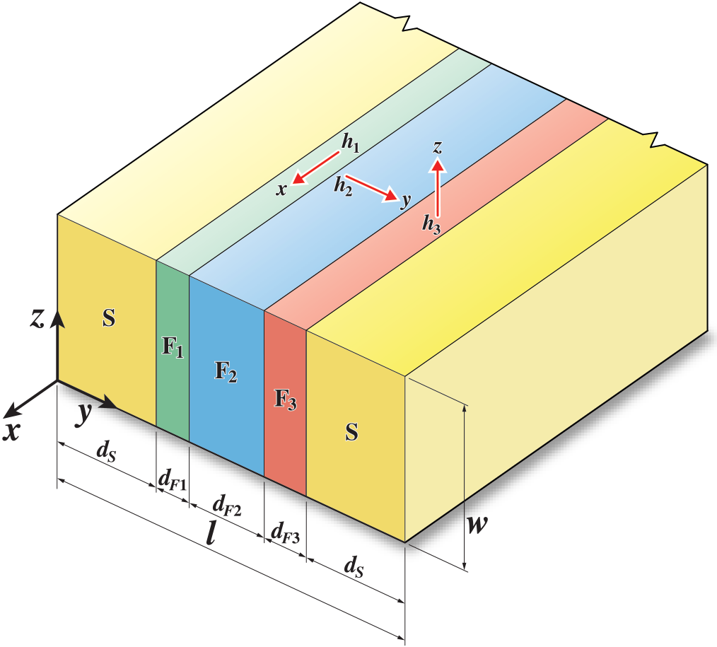
Figure 1: (Color online). Schematic of the F₁F₂F₃ ferromagnetic trilayer structure sandwiched between two $s$-wave superconductors ($\rm S$) with thickness $d_{S}$. The system is finite in the $y$-$z$ plane with width $w$ and length $l$, while infinite along $x$. The ferromagnets $\rm F_{i}\,(i=1,2,3)$ are of thicknesses $d_{Fi}$ and have arbitrary exchange-field strengths $h_{i}$. The typical magnetic configuration is shown here, where ${\bm{h}}_{1}$, ${\bm{h}}_{2}$, and ${\bm{h}}_{3}$ are oriented along the $x$, $y$, and $z$ directions, respectively (the ‘$xyz$’ configuration), although the exchange-field vectors can have arbitrary orientations determined by ${\bm{h}}_{i}=h_{i}(\cos\theta_{i},\sin\theta_{i}\sin\phi_{i},\sin\theta_{i}\cos\phi_{i})$.

II Methods

We first present the Hamiltonian, BdG formalism, the associated field operators, and Fourier expansion method in Sec. II.1. In Sec. II.2, the spin-singlet and spin-triplet correlations are given in terms of BdG transformations. The definitions and derivations of magnetic moment, DOS, charge current, and spin current and spin torque are presented in Secs. II.3, II.4, II.5, and II.6, respectively.

II.1 Hamiltonian

We now briefly summarize the BdG approach used to describe our spatially inhomogeneous nanostructure. We consider a Josephson configuration that is finite in the $y$-$z$ plane, and infinite in the $x$ direction [see Fig. 1]. The effective Hamiltonian ${\cal H}_{\rm eff}$ that describes this system is given by

$${\cal H}_{\rm eff} = \int d^{3}r\left\{\sum_{s}\psi_{s}^{\dagger}\left(\bm{r}\right)H_{0}\psi_{s}\left(\bm{r}\right)\right.$$ (1)

$$+ \left.\frac{1}{2}\left[\sum_{s\>s^{\prime}}\left(i\sigma_{y}\right)_{ss^{\prime}}\Delta\left(\bm{r}\right)\psi_{s}^{\dagger}\left(\bm{r}\right)\psi_{s^{\prime}}^{\dagger}\left(\bm{r}\right)+H.c.\right]\right.$$

$$- \left.\sum_{s\>s^{\prime}}\psi_{s}^{\dagger}\left(\bm{r}\right)\left(\bm{h}\cdot\bm{\sigma}\right)_{ss^{\prime}}\psi_{s^{\prime}}\left(\bm{r}\right)\right\},$$

where $s$ and $s^{\prime}$ are spin indices, and $\Delta({\bm{r}})$ is the pair potential, given by,

$$\Delta({\bm{r}})= \frac{V_{s}({\bm{r}})}{2}\left[\left\langle\psi_{\uparrow}({\bm{r}})\psi_{\downarrow}({\bm{r}})\right\rangle-\left\langle\psi_{\downarrow}({\bm{r}})\psi_{\uparrow}({\bm{r}})\right\rangle\right],$$ (2)

Here we have assumed an $s$-wave on-site potential with attractive interaction: $V({\bm{r}}-{\bm{r}^{\prime}})={V_{s}({\bm{r}})}\delta({\bm{r}}-{\bm{r}^{\prime}})$, with $V_{s}({\bm{r}})$ the interaction strength, which is nonzero only for energies less than a characteristic “Debye” energy, $\omega_{D}$, and nonzero only within the superconductor regions. The single-particle Hamiltonian $H_{0}$ for our finite-sized system in the two directions $y$ and $z$ [see Fig. 1] is written:

$$H_{0}=-\frac{1}{2m}\left(\frac{\partial^{2}}{\partial z^{2}}+\frac{\partial^{2}}{\partial y^{2}}\right)+\frac{1}{2m}k_{x}^{2}+U(y,z)-\mu,$$ (3)

in which $\mu$ is the Fermi energy, and $U(y,z)$ is the spin-independent scattering potential. The exchange field $\bm{h}\equiv(h_{x},h_{y},h_{z})$ describes the magnetic exchange interaction, and $\bm{\sigma}\equiv(\sigma_{x},\sigma_{y},\sigma_{z})$ are Pauli matrices. To diagonalize ${\cal H}_{\rm eff}$, the field operators $\psi_{s}$ and $\psi_{s}^{\dagger}$ are expanded by means of the Bogoliubov transformation:

$$\psi_{\uparrow}({\bm{r}}) =\sum_{n}\left(u_{n\uparrow}({\bm{r}})\gamma_{n}-v^{*}_{n\uparrow}({\bm{r}})\gamma_{n}^{\dagger}\right),$$ (4)

$$\psi_{\downarrow}({\bm{r}}) =\sum_{n}\left(u_{n\downarrow}({\bm{r}})\gamma_{n}+v^{*}_{n\downarrow}({\bm{r}})\gamma_{n}^{\dagger}\right),$$

where $u_{ns}$, $v_{ns}$ represent the quasiparticle amplitudes, and $\gamma_{n}$, $\gamma_{n}^{\dagger}$ are the Bogoliubov creation and annihilation operators, respectively. The transformations in Eq. (4) are required to diagonalize ${\cal H}_{\rm eff}$ such that,

$$\left[{\cal H}_{\rm eff},\gamma_{n}\right] =-\epsilon_{n}\gamma_{n},\quad\left[{\cal H}_{\rm eff},\gamma^{\dagger}_{n}\right] =\epsilon_{n}\gamma^{\dagger}_{n},$$ (5)

which leads to the spin-dependent Bogoliubov-de Gennes (BdG) equations as,

$$\begin{pmatrix}H_{0}-h_{z}(y,z)&-h_{x}(y,z)+ih_{y}(y,z)&0&\Delta(y,z)\\[5.0pt] -h_{x}(y,z)-ih_{y}(y,z)&H_{0}+h_{z}(y,z)&\Delta(y,z)&0\\[5.0pt] 0&\Delta^{*}(y,z)&-(H_{0}-h_{z}(y,z))&-h_{x}(y,z)-ih_{y}(y,z)\\[5.0pt] \Delta^{*}(y,z)&0&-h_{x}(y,z)+ih_{y}(y,z)&-(H_{0}+h_{z}(y,z))\\ \end{pmatrix}\left(\begin{array}[]{c}u_{n,\uparrow}(y,z)\\[5.0pt] u_{n,\downarrow}(y,z)\\[5.0pt] v_{n,\uparrow}(y,z)\\[5.0pt] v_{n,\downarrow}(y,z)\end{array}\right)=\epsilon_{n}\left(\begin{array}[]{c}u_{n,\uparrow}(y,z)\\[5.0pt] u_{n,\downarrow}(y,z)\\[5.0pt] v_{n,\uparrow}(y,z)\\[5.0pt] v_{n,\downarrow}(y,z)\end{array}\right),$$ (14)

The pair potential $\Delta(y,z)$ in Eq. (14) is assigned an initial value, taken to be the bulk gap, $\Delta_{0}$, in ${S_{1}}$ and $\Delta_{0}e^{i\varphi_{2}}$ in $S_{2}$, so that the macroscopic phase difference is $\Delta\varphi=\varphi_{2}$. We will investigate zero-phase (“anomalous”) spin and charge currents for $\Delta\varphi=0^{\circ}$, as well as controllable Josephson $\varphi_{0}$ states that occur when the ground state of the system occurs when $\Delta\varphi=\varphi_{0}$ (where $\varphi_{0}$ does not necessarily equal 0 or $\pi$). The ferromagnetic exchange field vector has its components expressed as:

$${\bm{h}}_{i}=h_{i}(\cos\theta_{i},\sin\theta_{i}\sin\phi_{i},\sin\theta_{i}\cos\phi_{i}),$$ (15)

where $i=1,2,3$ denotes the ferromagnetic region shown in Fig. 1. With these inputs, Eq. (14) is then numerically diagonalized to give the quasiparticle eigenenergies $\epsilon_{n}$ and the quasiparticle eigenfunctions ($u_{n\sigma}(y,z)$, $v_{n\sigma}(y,z)$). throughout the entire junction [79]. Since the structure in Fig. 1 is finite in the $y$ and $z$ directions, we solve the BdG equations by expanding the quasiparticle wavefunctions in a two-dimensional Fourier series basis,

$$u_{n,\sigma}(y,z) =\dfrac{2}{\sqrt{wl}}\sum^{N_{l}}_{p}\sum^{N_{w}}_{q}u^{p,q}_{n,\sigma}\sin\Big{(}\frac{p\pi y}{l}\Big{)}\sin\Big{(}\frac{q\pi z}{w}\Big{)},$$ (16)

$$v_{n,\sigma}(y,z) =\dfrac{2}{\sqrt{wl}}\sum^{N_{l}}_{p}\sum^{N_{w}}_{q}v^{p,q}_{n,\sigma}\sin\Big{(}\frac{p\pi y}{l}\Big{)}\sin\Big{(}\frac{q\pi z}{w}\Big{)},$$

where $\sigma=\uparrow,\downarrow$. Further details on this method can be found in Appendix A

II.2 Triplet correlations and pair amplitude

As discussed in Introduction, when strong ferromagnetic layers, such as half-metals, are part of a Josephson junction, the spin-triplet Cooper pairs can play an important role in both the thermodynamic and transport properties of the system [29, 74]. We begin by writing the spin triplet pairing correlations in the usual way [69],

$${f_{0}}({\bm{r}},t)= \frac{1}{2}\left[\left\langle\psi_{\uparrow}({\bm{r}},t)\psi_{\downarrow}({\bm{r}},0)\right\rangle+\left\langle\psi_{\downarrow}({\bm{r}},t)\psi_{\uparrow}({\bm{r}},0)\right\rangle\right],$$ (17a)

$${f_{1}}({\bm{r}},t)= \frac{1}{2}\left[\left\langle\psi_{\uparrow}({\bm{r}},t)\psi_{\uparrow}({\bm{r}},0)\right\rangle-\left\langle\psi_{\downarrow}({\bm{r}},t)\psi_{\downarrow}({\bm{r}},0)\right\rangle\right],$$ (17b)

$${f_{2}}({\bm{r}},t)= \frac{1}{2}\left[\left\langle\psi_{\uparrow}({\bm{r}},t)\psi_{\uparrow}({\bm{r}},0)\right\rangle+\left\langle\psi_{\downarrow}({\bm{r}},t)\psi_{\downarrow}({\bm{r}},0)\right\rangle\right],$$ (17c)

where the subscript $0$ corresponds to $m_{s}=0$, and the subscripts $1$ and $2$ refer to the $m_{s}=\pm 1$ projections on the spin quantization axis [30, 70]. It was shown in the previous works that using this approach to find both the opposite-spin and equal-spin triplet pairs, satisfy the Pauli exclusion principle, and that the spin triplet pairs vanish at $t=0$. If the exchange fields between the $\rm F$ layers are not aligned, the total spin operator of the pairs does not commute with the effective Hamiltonian, and the spin-polarized components $f_{1}$ and $f_{2}$ acquire nonzero values.

As mentioned earlier, the pair potential gives valuable information regarding the superconducting correlations within the superconductors only, as it vanishes outside of those regions where $V_{s}({\bm{r}})=0$. To reveal the fullest details of the spin singlet correlations throughout the entire system, which includes proximity effects between layers, we evaluate the pair amplitude from Eq. (2), $f_{3}={\Delta({\bm{r}})}/{V_{s}({\bm{r}})}$. Inserting the Bogoliubov expansions (Eq. (4)) into Eq. (2) gives the pair amplitude $f_{3}(y,z)$ in terms of the quasiparticle amplitudes:

$$f_{3}({y,z}){=}\frac{1}{4}\sum_{n}\big{[}u_{n\uparrow}({y,z})v^{*}_{n\downarrow}({y,z}){+}u_{n\downarrow}({y,z})v^{*}_{n\uparrow}({y,z})\big{]}\tanh\Big{(}\frac{\epsilon_{n}}{2T}\Big{)},$$ (18)

where the sum is cut off for states with energies that exceed $\omega_{D}$. Here the identity $1-2f(\varepsilon)=\tanh(\varepsilon/2T)$ has been used ($f$ is the Fermi function), along with the expectation values: $\langle\gamma^{\dagger}_{n}\gamma_{m}\rangle=\delta_{nm}f(\epsilon_{n})$, $\langle\gamma_{m}\gamma_{n}^{\dagger}\rangle=\delta_{nm}(1-f(\epsilon_{n}))$, and $\langle\gamma_{n}\gamma_{m}\rangle=0$.

To express the spin triplet correlations [Eqs. (17)] in terms of the quasiparticle energies and amplitudes, we first write the Heisenberg equations of motion for the Bogoliubov creation and annihilation operators: $i{\partial\gamma_{n}}/{\partial t}=[\gamma_{n},{\cal H}_{\rm eff}]$, $i{\partial\gamma^{\dagger}_{n}}/{\partial t}=[\gamma^{\dagger}_{n},{\cal H}_{\rm eff}]$. Using the conditions in Eq. (5), we have the solutions, $\gamma_{n}(t)=\gamma_{n}e^{-i\epsilon_{n}t}$ and $\gamma^{\dagger}_{n}(t)=\gamma^{\dagger}_{n}e^{i\epsilon_{n}t}$. Inserting these solutions into the generalized Bogoliubov transformations [Eq. (4)], it becomes possible to write the field operators in Eqs. (17)

$$f_{0}(y,z,t) =\frac{1}{2}\sum_{n}\left[u_{n\uparrow}(y,z)v^{\ast}_{n\downarrow}(y,z)-u_{n\downarrow}(y,z)v^{\ast}_{n\uparrow}(y,z)\right]\zeta_{n}(t),$$ (19a)

$$f_{1}(y,z,t) =-\frac{1}{2}\sum_{n}\left[u_{n\uparrow}(y,z)v^{\ast}_{n\uparrow}(y,z)+u_{n\downarrow}(y,z)v^{\ast}_{n\downarrow}(y,z)\right]\zeta_{n}(t),$$ (19b)

$$f_{2}(y,z,t) =-\frac{1}{2}\sum_{n}\left[u_{n\uparrow}(y,z)v^{\ast}_{n\uparrow}(y,z)-u_{n\downarrow}(y,z)v^{\ast}_{n\downarrow}(y,z)\right]\zeta_{n}(t),$$ (19c)

where the sums are over all energy values, and $\zeta_{n}(t)\equiv\cos(\epsilon_{n}t)-i\sin(\epsilon_{n}t)\tanh(\epsilon_{n}/2T)$. It can be more insightful to find the triplet correlations projected along the local spin axis [71], as dictated by the exchange field direction, instead of along the conventional $z$ direction. Performing the requisite spin rotations, we find:

$$f_{0}^{\prime} =f_{0}\cos\phi\sin\theta-f_{1}\cos\theta-if_{2}\sin\theta\sin\phi,$$ (20)

$$f_{1}^{\prime} =f_{0}\cos\theta\cos\phi+f_{1}\sin\theta-if_{2}\cos\theta\sin\phi,$$ (21)

$$f_{2}^{\prime} =-if_{0}\sin\phi+f_{2}\cos\phi.$$ (22)

Thus, e.g., considering the principle axes, we have for along $x$ ($\theta=0^{\circ}$, $\phi=0^{\circ}$): $f_{0}^{\prime}=-f_{1}$, $f_{1}^{\prime}=f_{0}$, and $f_{2}^{\prime}=f_{2}$. For along $y$ ($\theta=90^{\circ}$, $\phi=90^{\circ}$): $f_{0}^{\prime}=-if_{2}$, $f_{1}^{\prime}=f_{1}$, and $f_{2}^{\prime}=-if_{0}$, and finally, along the quantization $z$ axis ($\theta=90^{\circ}$, $\phi=0^{\circ}$), all spin triplet components are unchanged: $f_{0}^{\prime}=f_{0}$, $f_{1}^{\prime}=f_{1}$, $f_{2}^{\prime}=f_{2}$. The spin singlet pair amplitude $f_{3}$ is always invariant under spin rotations.

II.3 Magnetic moment

In our structures spin transport is influenced by the leakage of magnetic moment out of the $\rm F$ layers and into the superconductors. This can be characterized by the local magnetic moment ${\bm{m}}({\bm{r}})$,

$${\bm{m}}({\bm{r}})=-\mu_{B}\,\langle{\bm{\eta}}({\bm{r}})\rangle,$$ (23)

where ${\bm{\eta}}({\bm{r}})$ is the spin density operator,

$${\bm{\eta}}({\bm{r}})=\psi^{\dagger}({\bm{r}}){\mbox{\boldmath$\sigma$}}\psi({\bm{r}}),$$ (24)

and $\mu_{B}$ the Bohr magneton. Again, by using the generalized Bogoliubov transformation, each component of ${\bm{m}}$ can be written in terms of the quasiparticle and quasihole wavefunctions:

$$m_{x}(y,z) =-2\mu_{B}\sum_{n}{\rm Re}\Big{[}u_{n\uparrow}(y,z)u_{n\downarrow}^{\ast}(y,z)f(\epsilon_{n})$$

$$-v_{n\uparrow}(y,z)v_{n\downarrow}^{\ast}(y,z)(1-f(\epsilon_{n}))\Big{]},$$ (25a)

$$m_{y}(y,z) =2\mu_{B}\sum_{n}{\rm Im}\Big{[}u_{n\uparrow}(y,z)u_{n\downarrow}^{\ast}(y,z)f(\epsilon_{n})$$

$$+v_{n\uparrow}(y,z)v_{n\downarrow}^{\ast}(y,z)(1-f(\epsilon_{n}))\Big{]},$$ (25b)

$$m_{z}(y,z)= -\mu_{B}\sum_{n}\Bigg{[}\left(\left|u_{n\uparrow}(y,z)\right|^{2}-\left|u_{n\downarrow}(y,z)\right|^{2}\right)f(\epsilon_{n})$$

$$+\left(\left|v_{n\uparrow}(y,z)\right|^{2}-\left|v_{n\downarrow}(y,z)\right|^{2}\right)(1-f(\epsilon_{n}))\Bigg{]}.$$ (25c)

II.4 Density of states

The proximity-induced electronic density of states (DOS) can reveal signatures of the energy gap and localized Andreev bound states. One important experimental quantity involves tunneling spectroscopy experiments which can probe the local single particle spectra encompassing the proximity-induced DOS. The total DOS, $N(y,z,\varepsilon)$ is the sum $N_{\uparrow}(y,z,\varepsilon)+N_{\downarrow}(y,z,\varepsilon)$, involving the spin-resolved local DOS $N_{\sigma}(y,z,\varepsilon)$:

$$N_{\sigma}(y,z,\varepsilon)\!=\!-\!\sum_{n}\Biggl{[}|u_{n\sigma}(y,z)|^{2}f^{\prime}(\varepsilon\!-\!\epsilon_{n})+|v_{n\sigma}(y,z)|^{2}f^{\prime}(\varepsilon\!+\!\epsilon_{n})\Biggr{]},$$ (26)

where $f^{\prime}(\varepsilon)=\partial f/\partial\varepsilon$ is the derivative of the Fermi function, $f(\varepsilon)=(e^{\varepsilon/T}+1)^{-1}$. It is also convenient to use the following relation: $f^{\prime}(\varepsilon)=-1/(4T\cosh^{2}(\varepsilon/(2T))$. The sum above is over the quasiparticle amplitudes and eigenenergies $\epsilon_{n}$. Thus, the DOS calculated in Eq. (26) can provide both a spatial mapping and energy-resolved characterization of the number of quasiparticle states in Josephson junctions.

II.5 Charge transport

For the system shown in Fig. 1, we compute the supercurrent in the $y$ and $z$ directions by starting with the Heisenberg equation for the charge density $\rho({\bm{r}})$: ${{\partial}_{t}\left\langle\rho({\bm{r}})\right\rangle=i\left\langle\left[{\cal H}_{\rm eff},\rho({\bm{r}})\right]\right\rangle}$, where,

$$\rho({\bm{r}})= 2\sum_{n}\Biggl{[}\left(|u_{n\uparrow}({\bm{r}})|^{2}+|u_{n\downarrow}({\bm{r}})|^{2}\right)f(\epsilon_{n})$$

$$+\left(|v_{n\uparrow}({\bm{r}})|^{2}+|v_{n\downarrow}({\bm{r}})|^{2}\right)\left(1-f(\epsilon_{n})\right)\Biggr{]}.$$ (27)

The continuity equation for the charge supercurrent density ${\bm{J}}$ in the ferromagnetic junction region is written

$$\frac{\partial}{\partial t}\left\langle\rho(\bm{r})\right\rangle+\nabla\cdot{\bm{J}}=0,$$ (28)

where each component $J_{i}$ ($i=y,z$) is given by,

$$J_{i}=-\frac{e}{m}\!\sum_{n}{\rm Im}\Biggl{\{}\left[u_{n\uparrow}(y,z)\partial_{i}u^{*}_{n\uparrow}(y,z)+u_{n\downarrow}(y,z)\partial_{i}u^{*}_{n\downarrow}(y,z)\right]f(\epsilon_{n})+\left[v_{n\uparrow}(y,z)\partial_{i}v^{*}_{n\uparrow}(y,z)+v_{n\downarrow}(y,z)\partial_{i}v^{*}_{n\downarrow}(y,z)\right]\left(1-f(\epsilon_{n})\right)\Biggr{\}},$$ (29)

For the trilayer in the steady state, i.e., $\partial_{t}\left\langle\rho(\bm{r})\right\rangle=0$, we have numerically verified $\nabla\cdot{\bm{J}}=0$ when calculating current-phase-relations.

II.6 Spin transport

We now extend the above considerations to spin transport. As in the case of the charge density, the Heisenberg picture is utilized to determine the time evolution of the spin density, ${\bm{\eta}}({\bm{r}},t)$, $\frac{\partial}{\partial t}\langle{\bm{\eta}}({\bm{r}},t)\rangle=i\langle[{\cal H}_{\rm eff},{\bm{\eta}}({\bm{r}},t)]\rangle$, where ${\bm{\eta}}$ is given in Eq. (24). The associated continuity equation now reads,

$$\frac{\partial}{\partial t}\langle{\bm{\eta}}({\bm{r}},t)\rangle+{\bm{\nabla}}\cdot{\bm{\mathcal{S}}} ={\bm{\tau}},$$ (30)

where ${\bm{\mathcal{S}}}$ is the spin current tensor. This fundamental conservation law balances the spin current gradients and the spin torque ${\bm{\tau}}$. The expression for the spin-current, ${\bm{\mathcal{S}}}$, is found from taking the commutator above Eq. (30) and inserting Eq. (1):

$${\bm{\mathcal{S}}}=-\frac{i}{2m}\Bigl{\langle}\psi^{\dagger}({\bm{r}}){\bm{\nabla}}{\bm{\sigma}}\psi({\bm{r}})-{\bm{\nabla}}\psi^{\dagger}({\bm{r}}){\bm{\sigma}}\psi({\bm{r}})\Bigr{\rangle},$$ (31)

where the tensor components ${\bm{\mathcal{S}}}_{\alpha\beta}$ represents spin current with spin $\beta$ flowing along the $\alpha$ direction in real-space. We can now expand each spin component of the spin current in terms of the quasiparticle amplitudes to obtain:

$${\cal{S}}_{yx}=-\frac{i}{2m}\sum_{n}\Biggl{\{}f_{n}\Bigl{[}u_{n\uparrow}^{*}\frac{\partial u_{n\downarrow}}{\partial y}+u_{n\downarrow}^{*}\frac{\partial u_{n\uparrow}}{\partial y}-u_{n\downarrow}\frac{\partial u^{*}_{n\uparrow}}{\partial y}-u_{n\uparrow}\frac{\partial u^{*}_{n\downarrow}}{\partial y}\Bigr{]}-(1-f_{n})\Bigl{[}v_{n\uparrow}\frac{\partial v^{*}_{n\downarrow}}{\partial y}+v_{n\downarrow}\frac{\partial v^{*}_{n\uparrow}}{\partial y}-v^{*}_{n\uparrow}\frac{\partial v_{n\downarrow}}{\partial y}-v^{*}_{n\downarrow}\frac{\partial v_{n\uparrow}}{\partial y}\Bigr{]}\Biggr{\}},$$ (32a)

$${\bm{S}}_{yy}=-\frac{1}{2m}\sum_{n}\Biggl{\{}f_{n}\Bigl{[}u_{n\uparrow}^{*}\frac{\partial u_{n\downarrow}}{\partial y}-u_{n\downarrow}^{*}\frac{\partial u_{n\uparrow}}{\partial y}-u_{n\downarrow}\frac{\partial u^{*}_{n\uparrow}}{\partial y}+u_{n\uparrow}\frac{\partial u^{*}_{n\downarrow}}{\partial y}\Bigr{]}-(1-f_{n})\Bigl{[}v_{n\uparrow}\frac{\partial v^{*}_{n\downarrow}}{\partial y}-v_{n\downarrow}\frac{\partial v^{*}_{n\uparrow}}{\partial y}+v^{*}_{n\uparrow}\frac{\partial v_{n\downarrow}}{\partial y}-v^{*}_{n\downarrow}\frac{\partial v_{n\uparrow}}{\partial y}\Bigr{]}\Biggr{\}},$$ (32b)

$${\bm{S}}_{yz}=-\frac{i}{2m}\sum_{n}\Biggl{\{}f_{n}\Bigl{[}u_{n\uparrow}^{*}\frac{\partial u_{n\uparrow}}{\partial y}-u_{n\uparrow}\frac{\partial u^{*}_{n\uparrow}}{\partial y}-u^{*}_{n\downarrow}\frac{\partial u_{n\downarrow}}{\partial y}+u_{n\downarrow}\frac{\partial u^{*}_{n\downarrow}}{\partial y}\Bigr{]}-(1-f_{n})\Bigl{[}-v_{n\uparrow}\frac{\partial v^{*}_{n\uparrow}}{\partial y}+v^{*}_{n\uparrow}\frac{\partial v_{n\uparrow}}{\partial y}+v_{n\downarrow}\frac{\partial v^{*}_{n\downarrow}}{\partial y}-v^{*}_{n\downarrow}\frac{\partial v_{n\downarrow}}{\partial y}\Bigr{]}\Biggr{\}},$$ (32c)

$${\cal{S}}_{zx}=-\frac{i}{2m}\sum_{n}\Biggl{\{}f_{n}\Bigl{[}u_{n\uparrow}^{*}\frac{\partial u_{n\downarrow}}{\partial z}+u_{n\downarrow}^{*}\frac{\partial u_{n\uparrow}}{\partial z}-u_{n\downarrow}\frac{\partial u^{*}_{n\uparrow}}{\partial z}-u_{n\uparrow}\frac{\partial u^{*}_{n\downarrow}}{\partial z}\Bigr{]}-(1-f_{n})\Bigl{[}v_{n\uparrow}\frac{\partial v^{*}_{n\downarrow}}{\partial z}+v_{n\downarrow}\frac{\partial v^{*}_{n\uparrow}}{\partial z}-v^{*}_{n\uparrow}\frac{\partial v_{n\downarrow}}{\partial z}-v^{*}_{n\downarrow}\frac{\partial v_{n\uparrow}}{\partial z}\Bigr{]}\Biggr{\}},$$ (32d)

$${\bm{S}}_{zy}=-\frac{1}{2m}\sum_{n}\Biggl{\{}f_{n}\Bigl{[}u_{n\uparrow}^{*}\frac{\partial u_{n\downarrow}}{\partial z}-u_{n\downarrow}^{*}\frac{\partial u_{n\uparrow}}{\partial z}-u_{n\downarrow}\frac{\partial u^{*}_{n\uparrow}}{\partial z}+u_{n\uparrow}\frac{\partial u^{*}_{n\downarrow}}{\partial z}\Bigr{]}-(1-f_{n})\Bigl{[}v_{n\uparrow}\frac{\partial v^{*}_{n\downarrow}}{\partial z}-v_{n\downarrow}\frac{\partial v^{*}_{n\uparrow}}{\partial z}+v^{*}_{n\uparrow}\frac{\partial v_{n\downarrow}}{\partial z}-v^{*}_{n\downarrow}\frac{\partial v_{n\uparrow}}{\partial z}\Bigr{]}\Biggr{\}},$$ (32e)

$${\bm{S}}_{zz}=-\frac{i}{2m}\sum_{n}\Biggl{\{}f_{n}\Bigl{[}u_{n\uparrow}^{*}\frac{\partial u_{n\uparrow}}{\partial z}-u_{n\uparrow}\frac{\partial u^{*}_{n\uparrow}}{\partial z}-u^{*}_{n\downarrow}\frac{\partial u_{n\downarrow}}{\partial z}+u_{n\downarrow}\frac{\partial u^{*}_{n\downarrow}}{\partial z}\Bigr{]}-(1-f_{n})\Bigl{[}-v_{n\uparrow}\frac{\partial v^{*}_{n\uparrow}}{\partial z}+v^{*}_{n\uparrow}\frac{\partial v_{n\uparrow}}{\partial z}+v_{n\downarrow}\frac{\partial v^{*}_{n\downarrow}}{\partial z}-v^{*}_{n\downarrow}\frac{\partial v_{n\downarrow}}{\partial z}\Bigr{]}\Biggr{\}},$$ (32f)

The introduction of spatial inhomogeneity in magnetization texture or inversion-breaking spin-orbit coupling result in a net spin current imbalance that is finite even in the absence of a Josephson current. [24, 72, 73]

To compute the spin torque, another approach involves using the continuity equation in the steady state to determine the spin torque by evaluating the derivatives of the spin current as a function of position. In the steady state, the continuity equation reads, ${\bm{\nabla}}\cdot{\bm{\mathcal{S}}}={\bm{\tau}}$. Since the structure is finite in the $y$ and $z$ directions, we have the following components of the torque vector:

$$\tau_{x}=\frac{\partial{\cal S}_{yx}}{\partial y}+\frac{\partial{\cal S}_{zx}}{\partial z},\,\tau_{y}=\frac{\partial{\cal S}_{yy}}{\partial y}+\frac{\partial{\cal S}_{zy}}{\partial z},\,\tau_{z}=\frac{\partial{\cal S}_{yz}}{\partial y}+\frac{\partial{\cal S}_{zz}}{\partial z}.$$ (33)

When the junctions are in static equilibrium and there is no charge current, the spin-current does not necessarily vanish because any inhomogeneous magnetization leads to a non-zero spin torque that generates a net spin current.

III Results and discussions

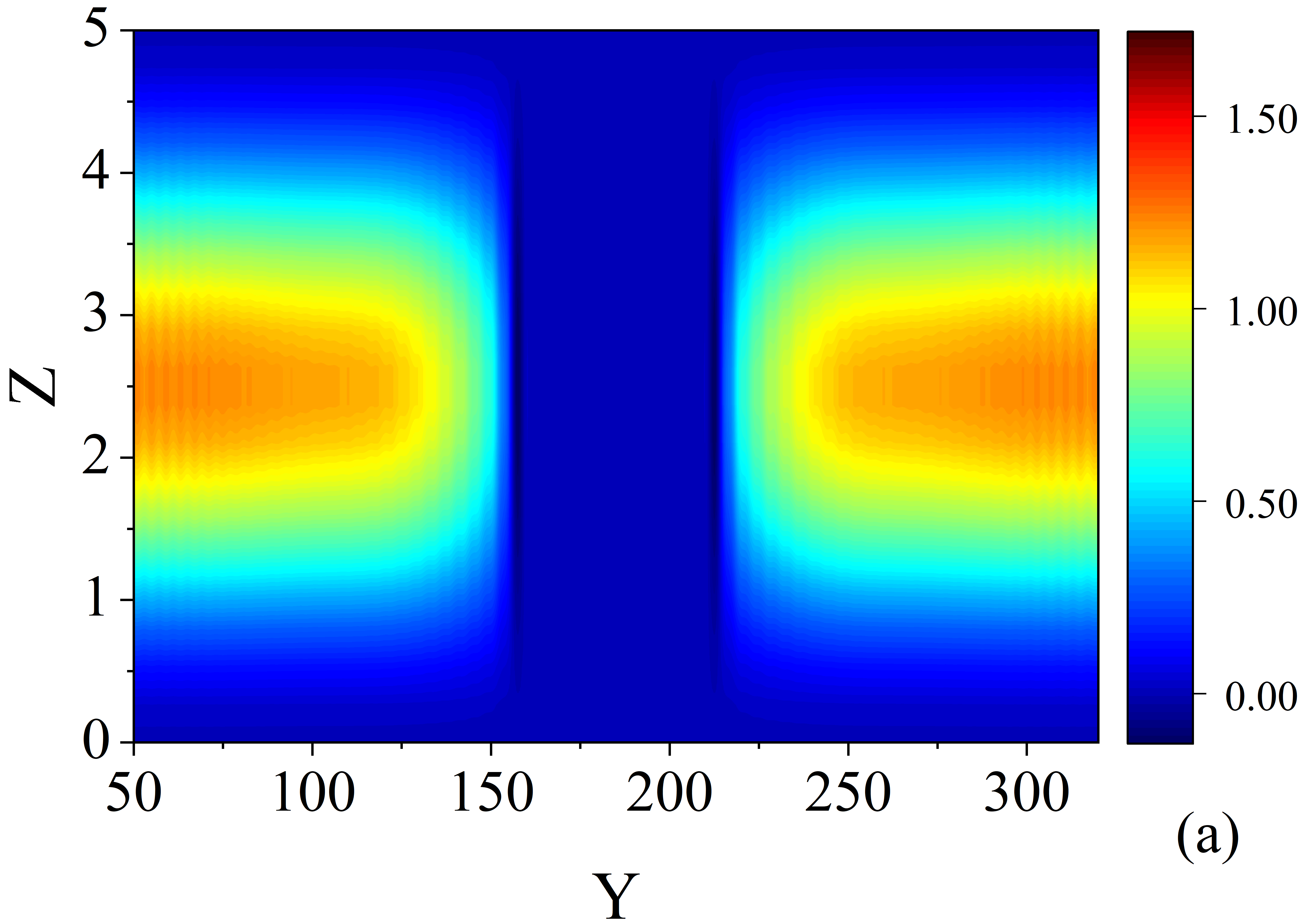
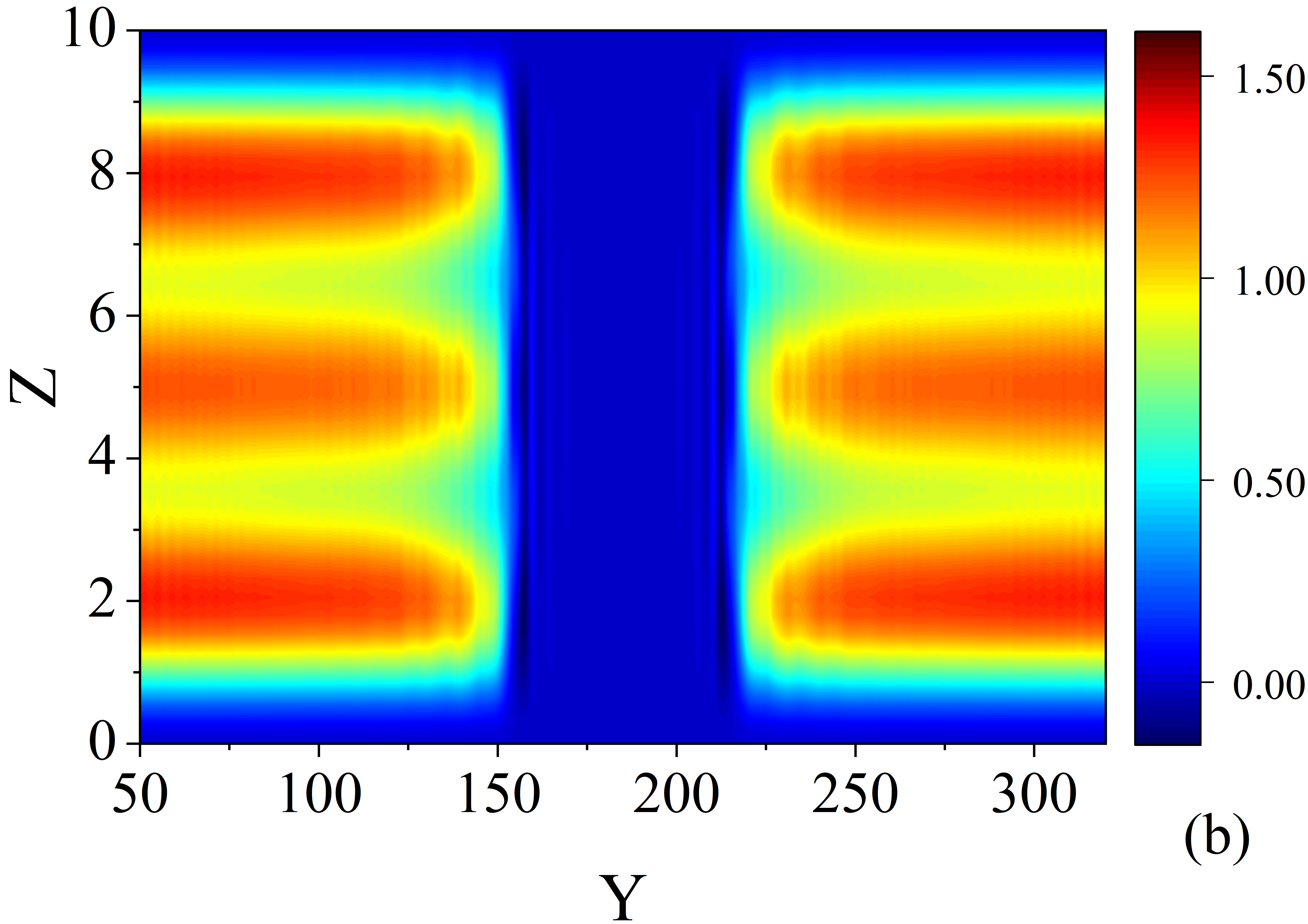
Figure 2: Pair amplitude for a half-metallic Josephson junction with an initial phase difference of $\Delta\varphi=0$. The exchange field magnitudes are set to $h_{1}=h_{3}=0.1E_{F}$, and $h_{2}=E_{F}$. The exchange fields in each ferromagnet are orthogonal to one another, i.e., directed along the $x$, $y$, and $z$ directions for $\rm F_{1}$, $\rm F_{2}$, and $\rm F_{3}$, respectively. The geometrical parameters are as follows: $D_{F1}=D_{F3}=10$, and $D_{F2}=50$. Three different widths $W$ are considered, $W=5$ [(a)], $W=10$, [(b)], and $W=50$ [(c)]. Spin triplet amplitudes $f_{0}$, $f_{1}$ and $f_{2}$ for the Josephson junction in panel (b). with an initial phase difference of $\Delta\varphi=0$, and relatively narrow width, $W=10$.

The results of our systematic investigations are presented below in terms of convenient dimensionless quantities. Our choices are as follows: all length scales, including the spatial coordinates $Y=k_{F}y$, $Z=k_{F}z$, and widths $D_{Fi}\equiv k_{F}d_{Fi}(i=1,2,3)$ are normalized by the Fermi wave-vector, $k_{F}$. For the superconducting correlation length $\xi$ we choose the value $k_{F}\xi_{0}=50$, and the computational region occupied by the S electrodes corresponds to a width of $k_{F}d_{S}=150$ (see Appendices A, B, and C for numerical details). The outer ferromagnet layers must be thin to effectively generate the spin-triplet correlations [24, 25, 71]. We found $D_{F1}=D_{F3}=10$ to be effective lengths for generating a large population of spin-triplet correlations. All temperatures are measured in units of $T_{c0}$, the transition temperature of bulk S material, and we consider the low temperature regime, $T/T_{c0}=0.05$, throughout the paper. Energy scales are normalized by the Fermi energy, $E_{F}$, including the Stoner energy $h_{i}$ and the energy cutoff, $\omega_{D}$, used in calculating the pair amplitude, Eq. (18). The latter is set at 0.1, with the main results relatively insensitive to this cutoff choice. The strength of the magnetic exchange fields, $h_{1,3}$ is taken to be the same in both magnets: we set its dimensionless value to a representative $h_{1,3}/E_{F}=0.1$. The exchange field in the central ferromagnet layer will typically correspond to a half-metal ($h_{2}=E_{F}$) but other exchange field strengths will be studied as well. The orientation angles of the magnetic exchange field in each of the ferromagnet regions can vary, depending on the quantity being studied, however most cases consider the $xyz$ configuration, whereby the exchange fields in $\rm F_{1}$, $\rm F_{2}$, and $\rm F_{3}$ are aligned on the $x$, $y$, and $z$ directions, respectively. All results for the DOS in this work are presented normalized to the superconductor’s normal state DOS at the Fermi level. The magnetization is normalized by $\mu_{B}n_{e}$, and the normalization $\tau_{0}$ for the spin torque follows from the normalizations for ${\bm{h}}_{i}$ and ${\bm{m}}$ in Eq. (35). For the transport quantities, we normalize the charge currents by $J_{0}$, where $J_{0}=en_{e}v_{F}$, $v_{F}=k_{F}/m$ is the Fermi velocity, obtained through dividing Fermi wave vector $k_{F}$ by the mass of quasiparticles $m$, and $n_{e}$ is the electron density, written as $n_{e}=k_{F}^{3}/(3\pi^{2})$. We focus on the supercurrent along the $y$ direction $J_{y}$, evaluated at $Z=W/2$, the center of the junction. Nearly identical results are found if $J_{y}$ is spatially integrated along the width $W$.

In describing inhomogeneous superconductivity in multilayer SF₁F₂F₃S Josephson structures, it is insightful to examine the spatial properties of the singlet correlations. Thus we present in Fig. 2, the real parts of the pair amplitudes $f_{3}$ normalized by their bulk value for three different geometrical configurations. Three different widths of the junction are shown: Figures 2(a) and 2(b) correspond to relatively narrow junctions with $W=5$, and $W=10$, respectively. Figure 2(c) is for a junction width of $W=50=k_{F}\xi_{0}$. The pair amplitudes are determined by summing the quasiparticle amplitudes and energies [Eq. (18)] calculated from Eq. (14). The central ferromagnet is half metallic ($h_{2}/E_{F}=1$) with a dimensionless width of $D_{F2}=50$. The exchange field vectors are oriented along the $x$, $y$, and $z$ directions in $\rm F_{1}$, $\rm F_{2}$, and $\rm F_{3}$, respectively (the $xyz$ configuration). Along the $y$ direction, the outer superconductors occupy the regions $0<Y<150$ and $220<Y<370$. Figures 2(a)-2(c), the pair amplitude vanishes in the half-metal region ($160<Y<210$), where only one spin channel is permitted. For the narrow channel Fig. 2(a), superconductivity reaches its maximal value along the midline of the width side ($Z=2.5$) and nearly vanishes in the vicinity of the outer boundaries ($Z=0,5$). Boundary and size-effects from quasiparticle reflections at the outer walls are mainly responsible for the observed contours. The number of peaks in the pair amplitude profiles is seen to increase for the wider junctions shown in Figs. 2(b) and 2(c), as electron trajectories involve larger paths, and interference effects become diminished.

The spatial behavior of the spin triplet correlations $f_{0}$, $f_{1}$, and $f_{2}$ are shown in the bottom row of Fig. 2. The system parameters are the same as those used for the $W=10$ case shown in Fig. 2(b). Beginning with the opposite-spin triplets $f_{0}$, Fig. 2(d) demonstrates that the regions occupied by the thin outer ferromagnets ($150<Y<160$ and $210<Y\leq 220$) contain a considerable enhancement of the $f_{0}$ triplet component that decays substantially in the other regions. The equal-spin triplet correlations $f_{1}$ and $f_{2}$ in Figs. 2(e,f) exhibit behavior that is strikingly different, where they permeate the entire half-metal ($160\leq Y\leq 210$) where spin-polarized pair correlations can survive. Moreover, the $f_{1}$ triplets are seen to propagate into the superconductor ($Y>220$) at the given time. Note that long-range transport of triplet pairs can occur in Josephson structures containing only two magnets, i.e., SF₁F₂F₃S junctions, as will be seen below, trilayer ferromagnet junctions are required to generate a spontaneous supercurrent with a zero phase difference $\Delta\varphi=0$.

Figure 3: (a) Normalized anomalous current $J_{y}(\Delta\varphi=0)$ versus the transverse width $W$. The lengths of the ferromagnet segments are as follows: $D_{F1}=D_{F3}=10$, and $D_{F2}=50$. In (b) the width $W=10$ is fixed, while the length of the central ferromagnet, $D_{F2}$, changes. The surrounding ferromagnets $\rm F_{1}$ and $\rm F_{3}$ have the same lengths as in (a). The junction for each scenario has a macroscopic phase difference of zero, $\Delta\varphi=0$, between the outer superconducting electrodes, and the exchange fields in the ferromagnets are all orthogonal to one another (i.e., the $xyz$ configuration)

As observed in Fig. 2, differing junction widths lead to considerable differences in the behavior of the singlet correlations. To examine how geometrical changes affect Cooper pair transport, we present in Figs. 3(a,b) the normalized supercurrent in the $y$ direction as a function of the normalized width $W$ and central ferromagnet layer thickness $D_{F2}$, respectively. Here we fix $\Delta\varphi=0$, and the middle ferromagnet is half-metallic, i.e., $h_{2}/E_{F}=1$. It was found theoretically and experimentally that equal-spin triplet pairs can result in a more robust Josephson supercurrent that has a weak sensitivity to ferromagnet layer thicknesses due to their long ranged nature [22, 74]. If one of the ferromagnets in the junction is half-metallic, the equal-spin triplet correlations are expected to play an even greater role in the behavior of the supercurrent. In Fig. 3(a) the zero-phase current is calculated for a wide range of junction widths $W$, while keeping the lengths fixed at $D_{F2}=50$ and $D_{F1}=D_{F3}=10$. It is evident that damped oscillatory quantum size-effects are discernible for $W\lesssim 30$. For larger $W$, the size-effects vanish, and the zero-phase current levels off at its bulk value. Related to this, oscillations over the Fermi length scale were observed in the critical temperatures of thin films, attributed to quantum size effects [75, 76]. Next, the normalized width is fixed to $W=10$, and the length of the central half-metal is varied. The spontaneous supercurrent vanishes when $D_{F2}=0$ since that leaves only two ferromagnets with orthogonal exchange fields. Increasing $D_{F2}$ leads to a rapid increase in the magnitude of $J_{y}(\Delta\varphi=0)$ that peaks at $D_{F2}\approx 10$. As $D_{F2}$ is increased further, the supercurrent tends towards zero slowly. This slow decay is indicative of a spin-polarized current flowing through the junction, as a current comprised of spin singlet pairs would decay completely within the half-metal region, supporting the strongest magnetization strength.

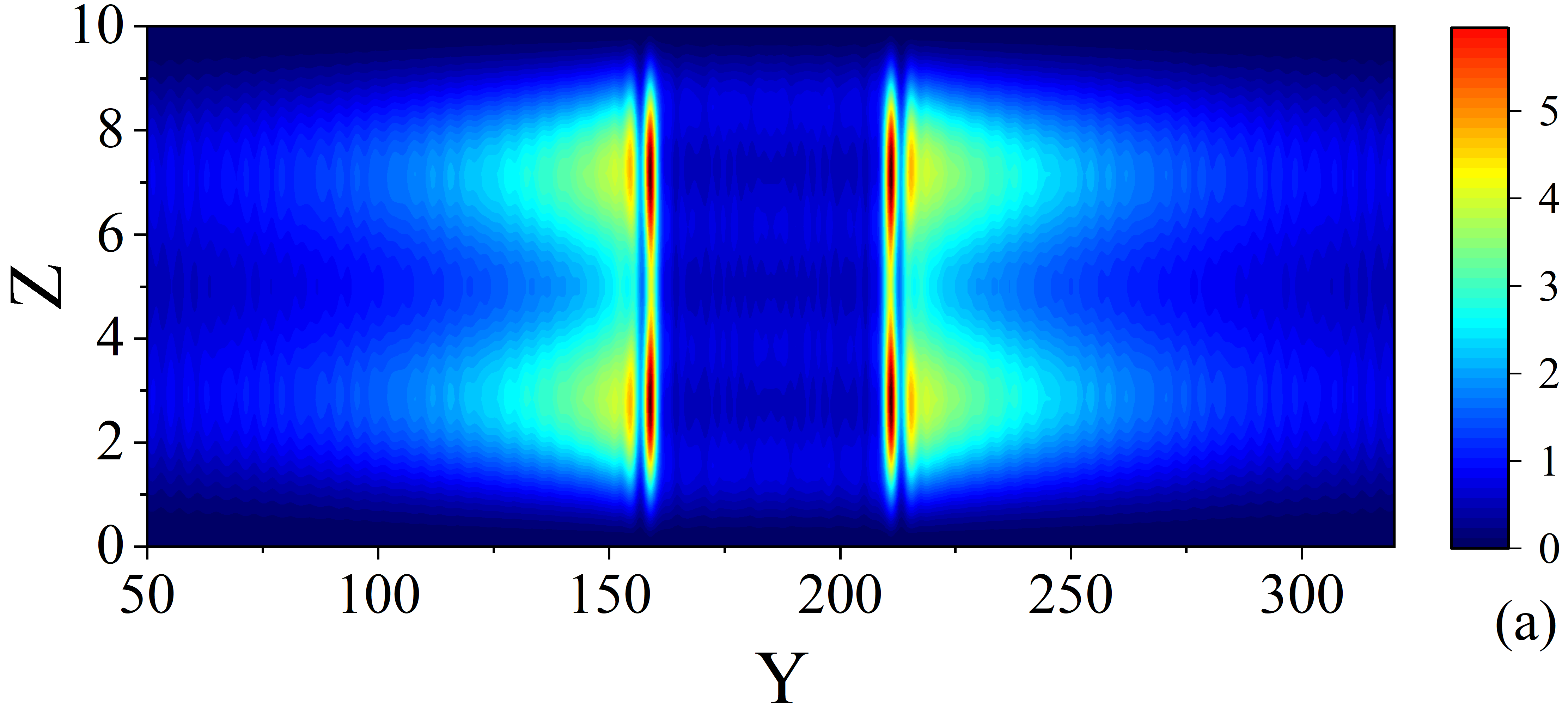
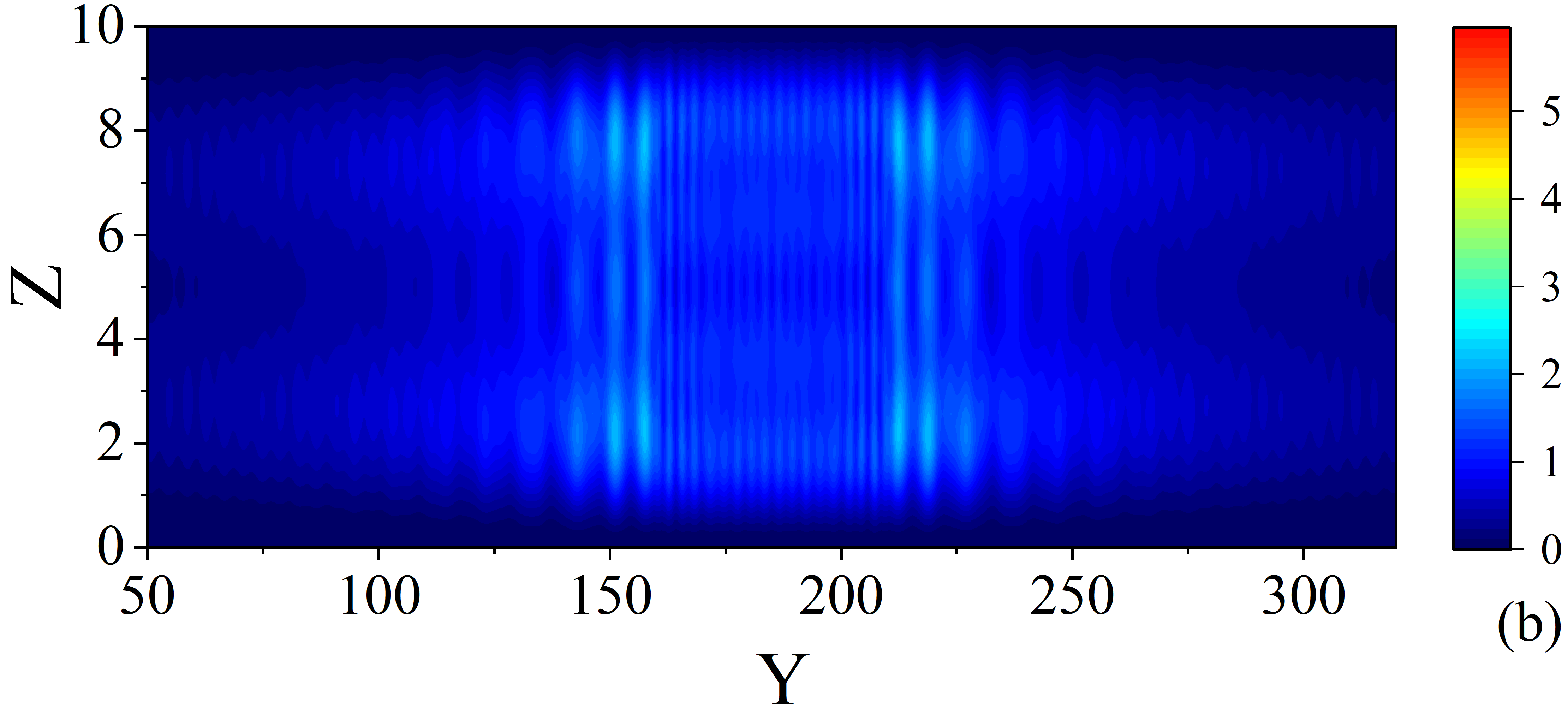
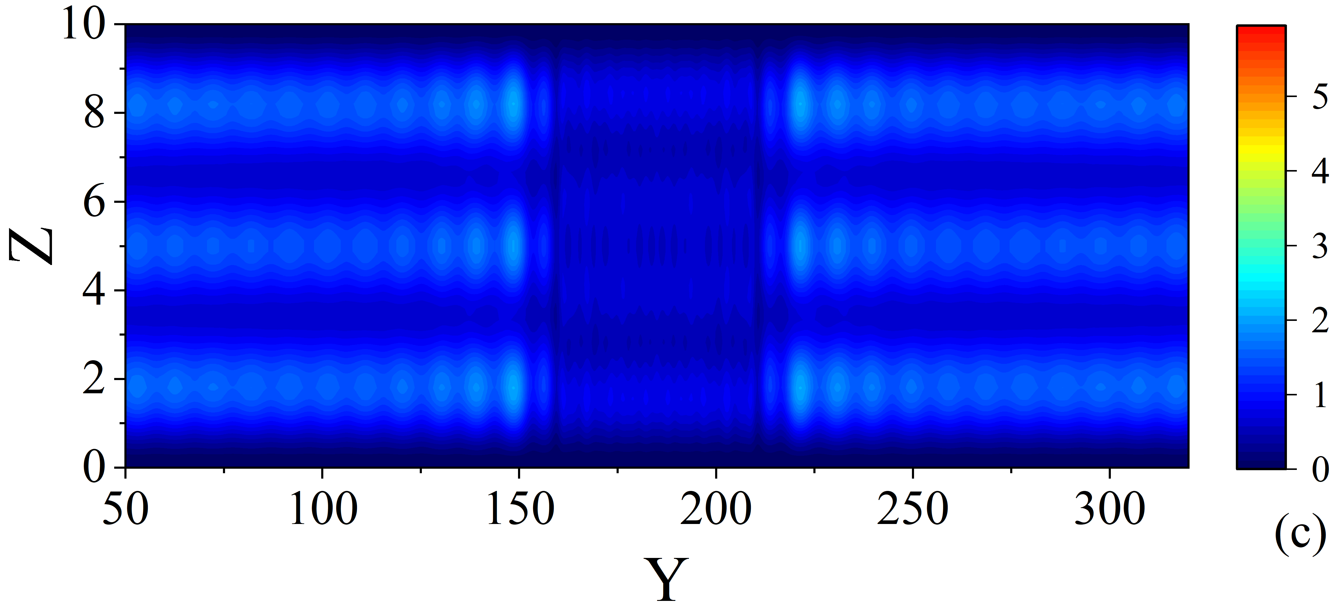
Figure 4: Local density of states at three different normalized energies: (a) $\epsilon/\Delta_{0}=0$, (b) $\epsilon/\Delta_{0}=0.5$, and (c) $\epsilon/\Delta_{0}=1$. An initial phase difference of $\Delta\varphi=0$ is considered. The exchange field of the central $\rm F$ layer is set to $h_{2}=E_{F}$, and the outer two magnets have $h_{1}=h_{3}=0.1E_{F}$. The exchange field orientations in each ferromagnet are orthogonal to one another, corresponding to the $x$, $y$, and $z$ directions for $\rm F_{1}$, $\rm F_{2}$, and $\rm F_{3}$, respectively. A narrow junction width is considered, with $W=10$.

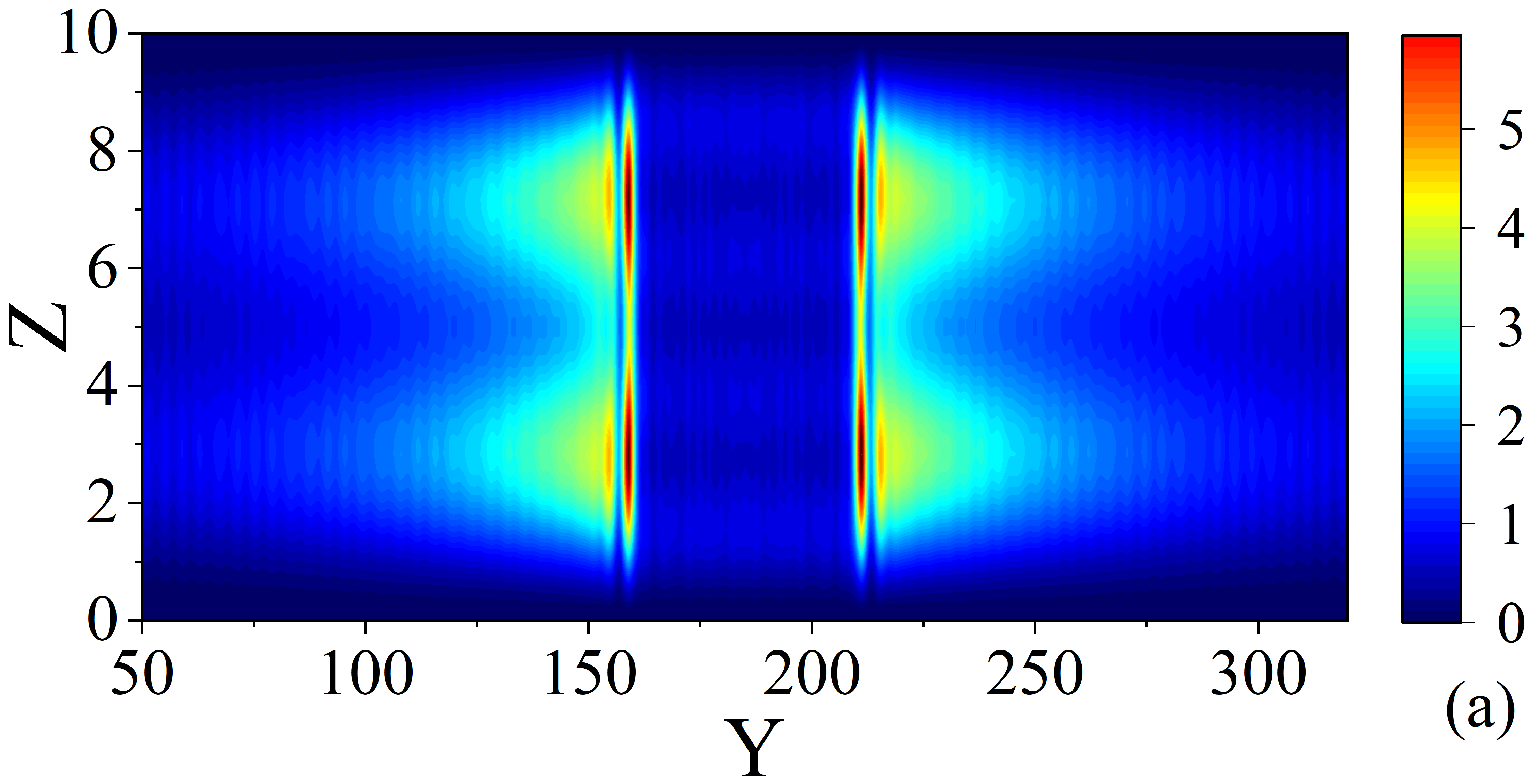
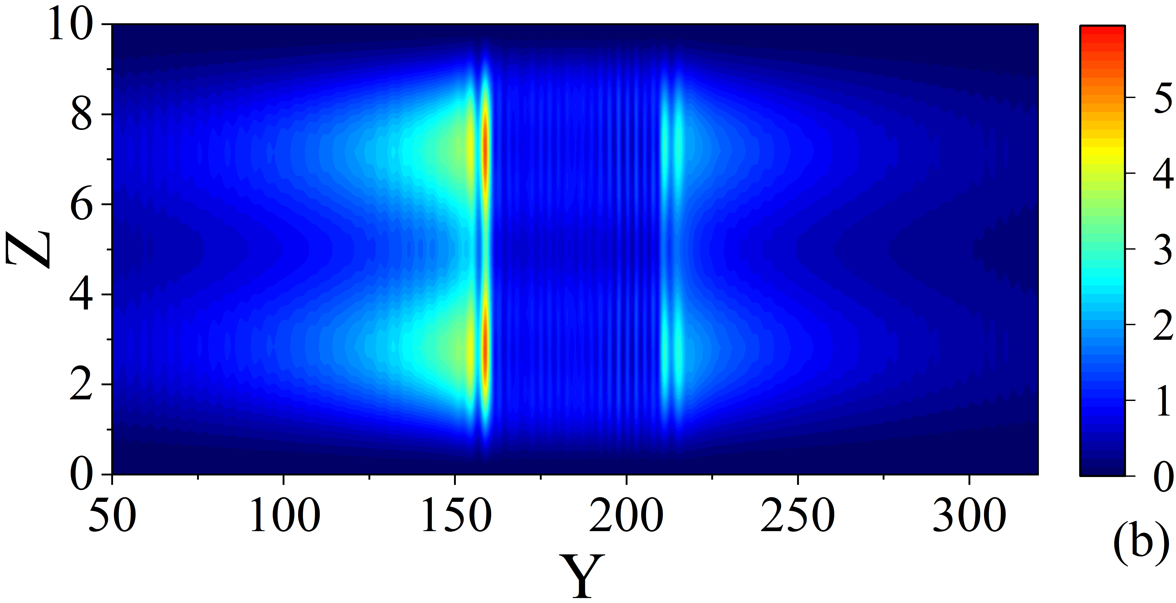
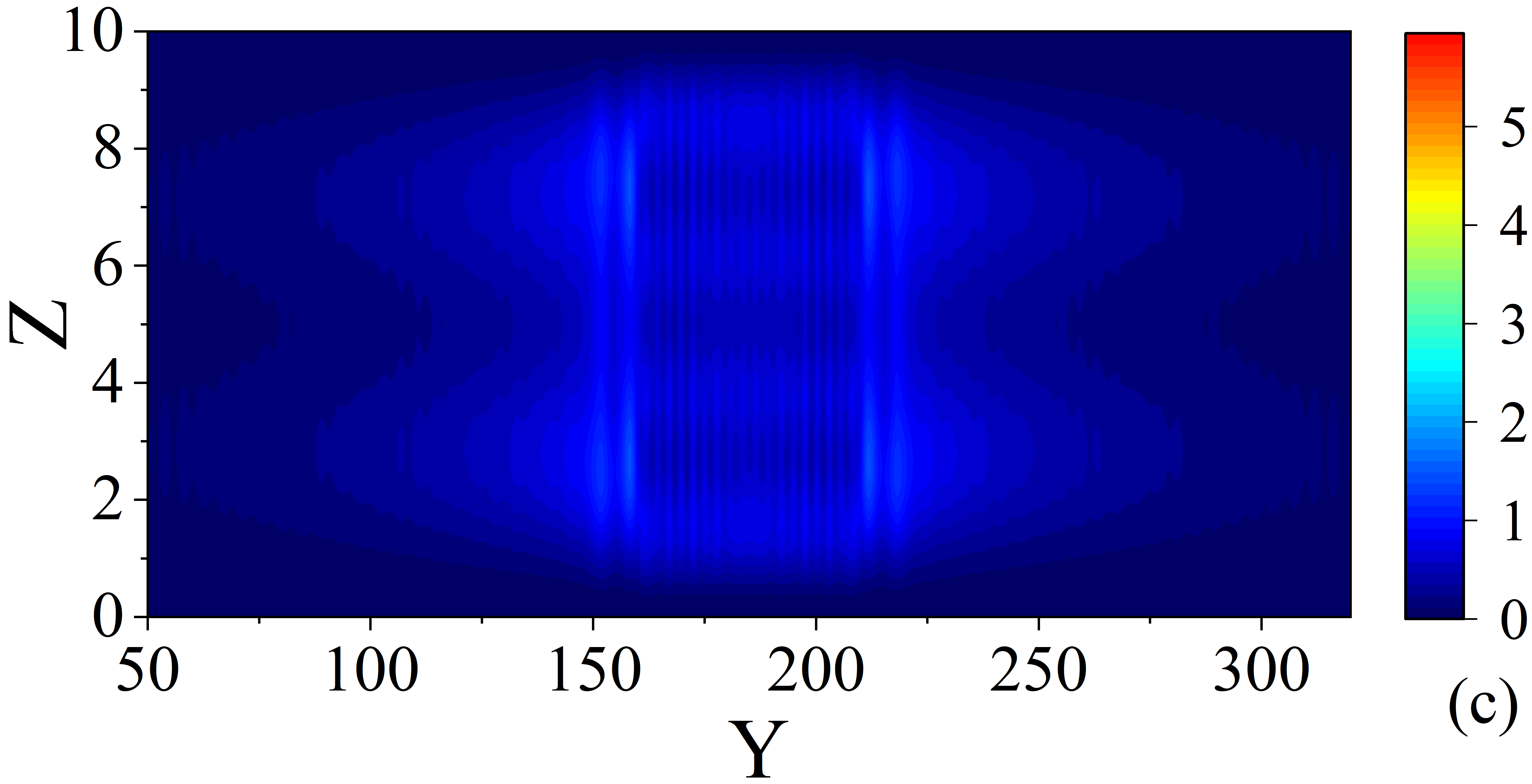
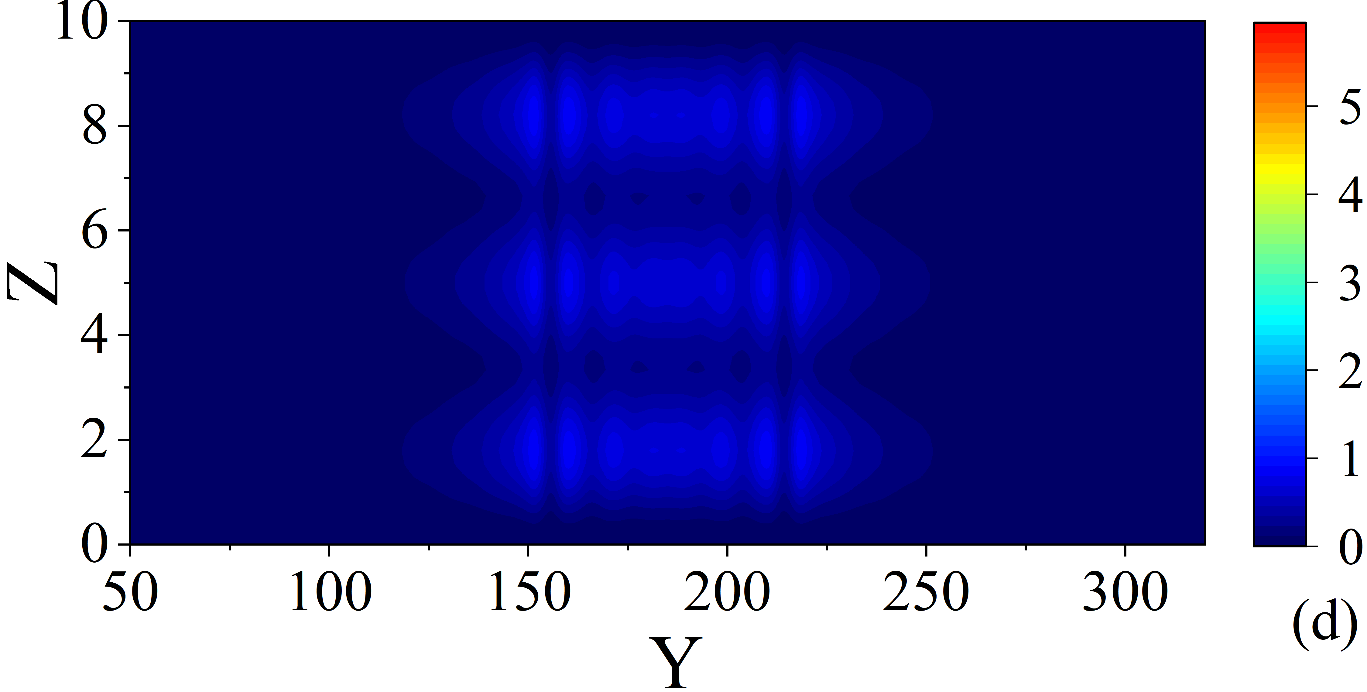
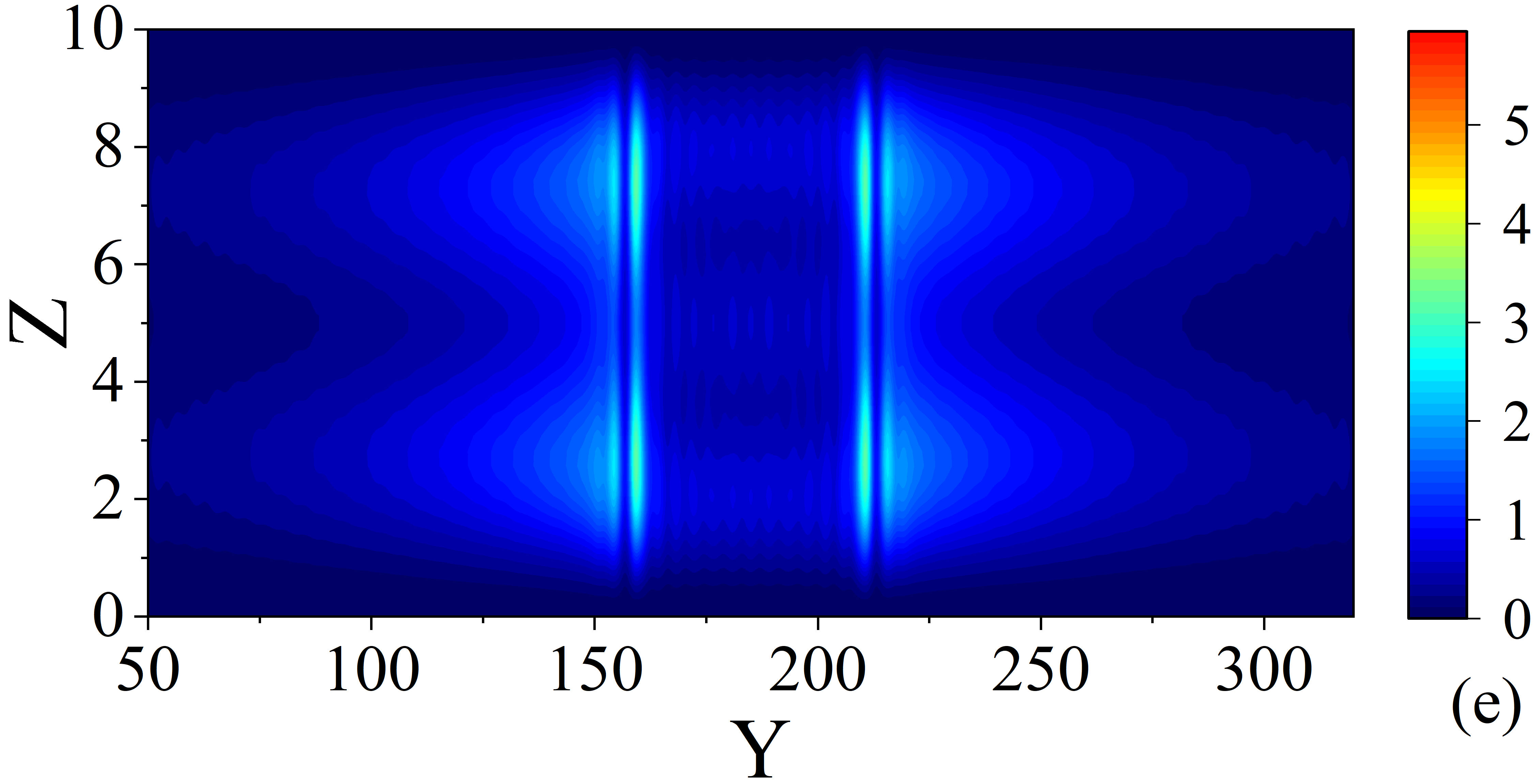
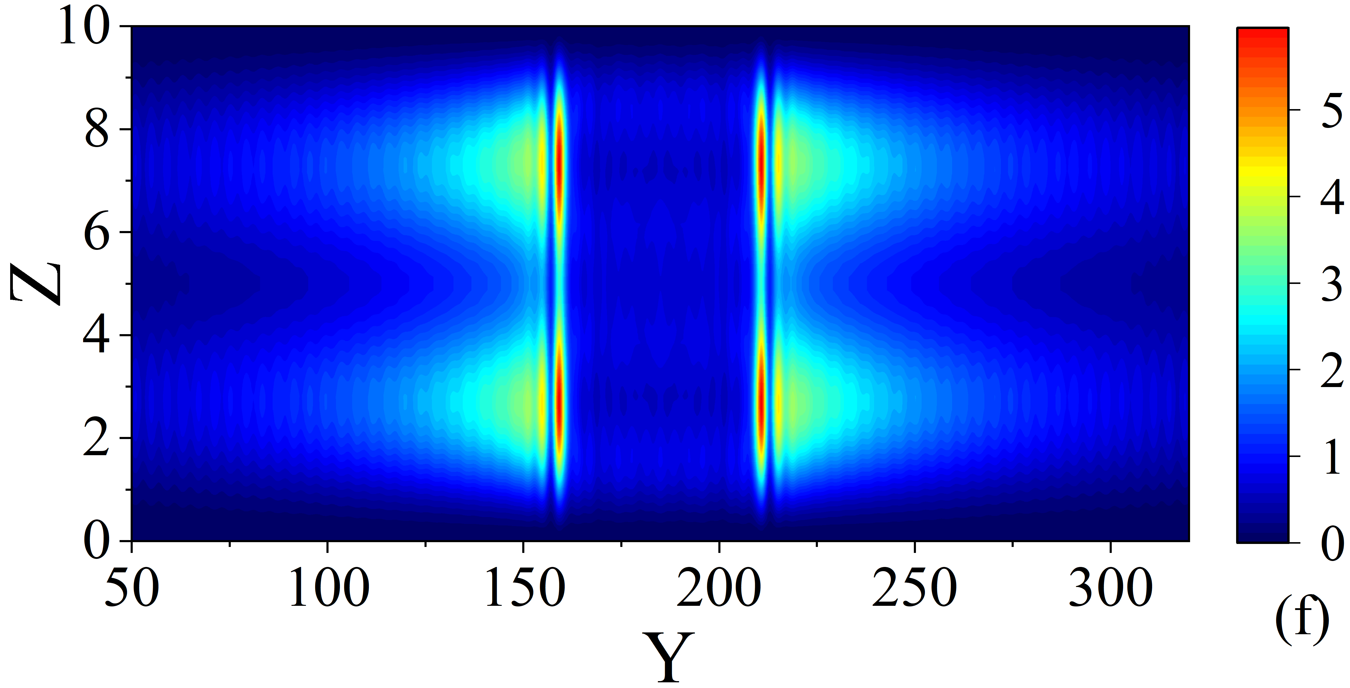
Figure 5: Local density of states at zero energy. Top row: Three different relative orientations of the exchange field in the outer ferromagnet $\rm F_{3}$ are considered: In (a),(b) ${\bm{h}}_{1}$ and ${\bm{h}}_{2}$ are directed along the $x$ and $y$ directions, respectively, while in (a) ${\bm{h}}_{3}$ is along $z$ ($\theta_{3}=90^{\circ}$,$\phi_{3}=0^{\circ}$), and (b) ${\bm{h}}_{3}$ is along $y$ ($\theta_{3}=90^{\circ}$,$\phi_{3}=90^{\circ}$). In (c), the exchange fields in all three magnets are aligned along the $y$ direction. An initial phase difference of $\Delta\varphi=0$ is assumed. The magnitude of the exchange field of the central $\rm F$ layer is set to $h_{2}=E_{F}$, and the outer two magnets have $h_{1}=h_{3}=0.1E_{F}$. A narrow junction width is considered, with $W=10$. Bottom row: Three different exchange fields in the central ferromagnet $\rm F_{2}$ are considered: (d) $h=0$, (e) $h=0.5$, and (f) $h=0.7$. A zero phase difference is considered, i.e., $\Delta\varphi=0$. The magnitude of the exchange field in the outer two magnets have $h_{1}=h_{3}=0.1E_{F}$. A narrow junction width is considered, with $W=10$.

The electronic density of states (DOS) provides another avenue for detecting signatures of single-particle localized Andreev states. The study of single-particle excitations in these systems can reveal indirect signatures of the proximity induced spin singlet and spin triplet pair correlations. Experimentally, this involves tunneling spectroscopy experiments which can probe the local proximity-induced DOS. From a theoretical perspective, it is revealing to study the DOS spatially throughout the entire junction at certain key energies. Thus in Figs. 4(a-c) the local DOS, normalized by the normal state DOS, $N_{0}$, is shown at three normalized energies. For $\epsilon/\Delta_{0}=0$ in Fig. 4(a) there is a considerable enhancement in the DOS in the vicinity of the interfaces separating the superconductors from the ferromagnetic junction region. In particular the DOS peaks within the weaker outer ferromagnets $\rm F_{1}$ and $\rm F_{3}$, and decays abruptly within the half-metallic region. There is a much slower decay within the superconductor regions. This profile is indicative of the generation of equal-spin triplet correlations. In Fig. 4(c) for $\epsilon/\Delta_{0}=1$, there are BCS-like peaks that exhibit quantum interference patterns due to the finite size of the junction. These peaks remain regular throughout the outer superconducting banks, and the DOS is much smaller in the ferromagnetic regions, where it is weak but nonzero as there is no energy gap for the parameters used here.

Having established the existence of strong zero energy peaks for the half-metallic junction with each of the exchange fields of the three magnets orthogonal to one another, we now examine the local DOS at zero energy for other orientation angles and magnitudes of the exchange field. In the top row of Fig. 5, the normalized exchange energy is set at $h_{2}/E_{F}=1$, while the angle $\phi_{3}$ is $\phi_{3}=0^{\circ}$ in Fig. 5(a) and $\phi_{3}=90^{\circ}$ in Fig. 5(b). In Fig. 5(c), each ferromagnet has its exchange field aligned along the $y$ direction. Clearly the most dominant zero energy peaks occur in Fig. 5(a) within the thin outer ferromagnets ($150<Y<160$ and $210<Y<220$) where the magnets are all orthogonal. In Fig. 5(b), the rightmost two magnets $\rm F_{1}$ and $\rm F_{2}$ (see Fig. 1) have their exchange field along the $y$ direction. This reduces the magnetic inhomogeneity, leading to an asymmetric profile for the quasiparticle excitations that is dominant on the left side. Finally in Fig. 5(c), when there exists the possibility to describe the system by a single spin-quantization axis, the spin-polarized triplet correlations vanish [70], and there is a strongly diminished DOS at zero energy. For the bottom row of Fig. 5, the ferromagnets are all fixed in the $xyz$ configuration, while the central exchange field strength is varied according to $h_{2}/E_{F}=0,0.5,0.7$ in Figs. 5(e-f), respectively. For the unpolarized normal metal case in Fig. 5(d), there is no zero energy peaks within the junction, but instead a series of weak, repeating bands that arise from proximity effects and a superposition of quasiparticle states confined by the outer superconductor banks. Increasing the exchange field to $h_{2}/E_{F}=0.5$ in Fig. 5(e), there is a slight development of zero energy states along the boundaries that becomes amplified for $h_{2}/E_{F}=0.7$ [Fig. 5(f)].

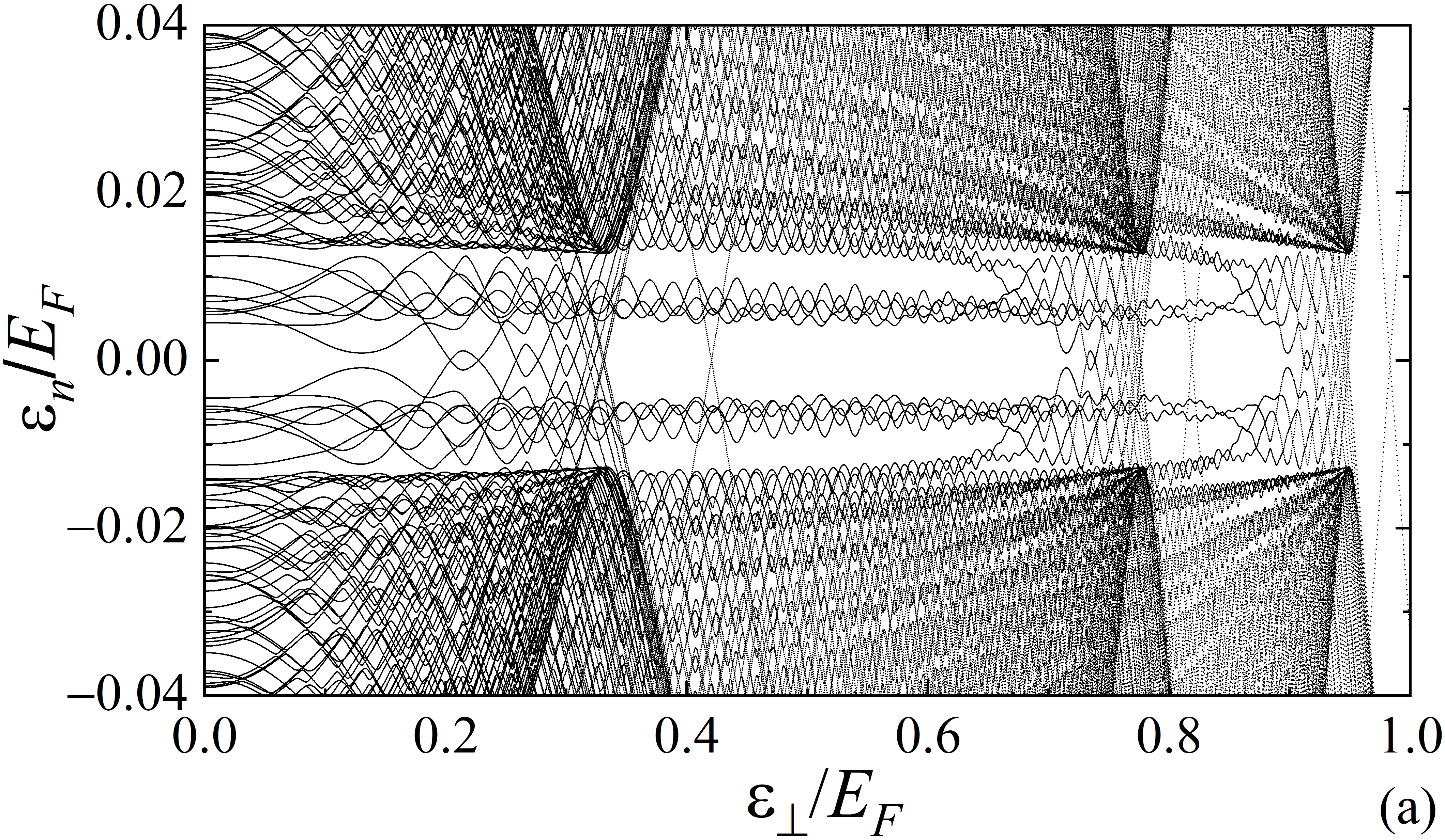
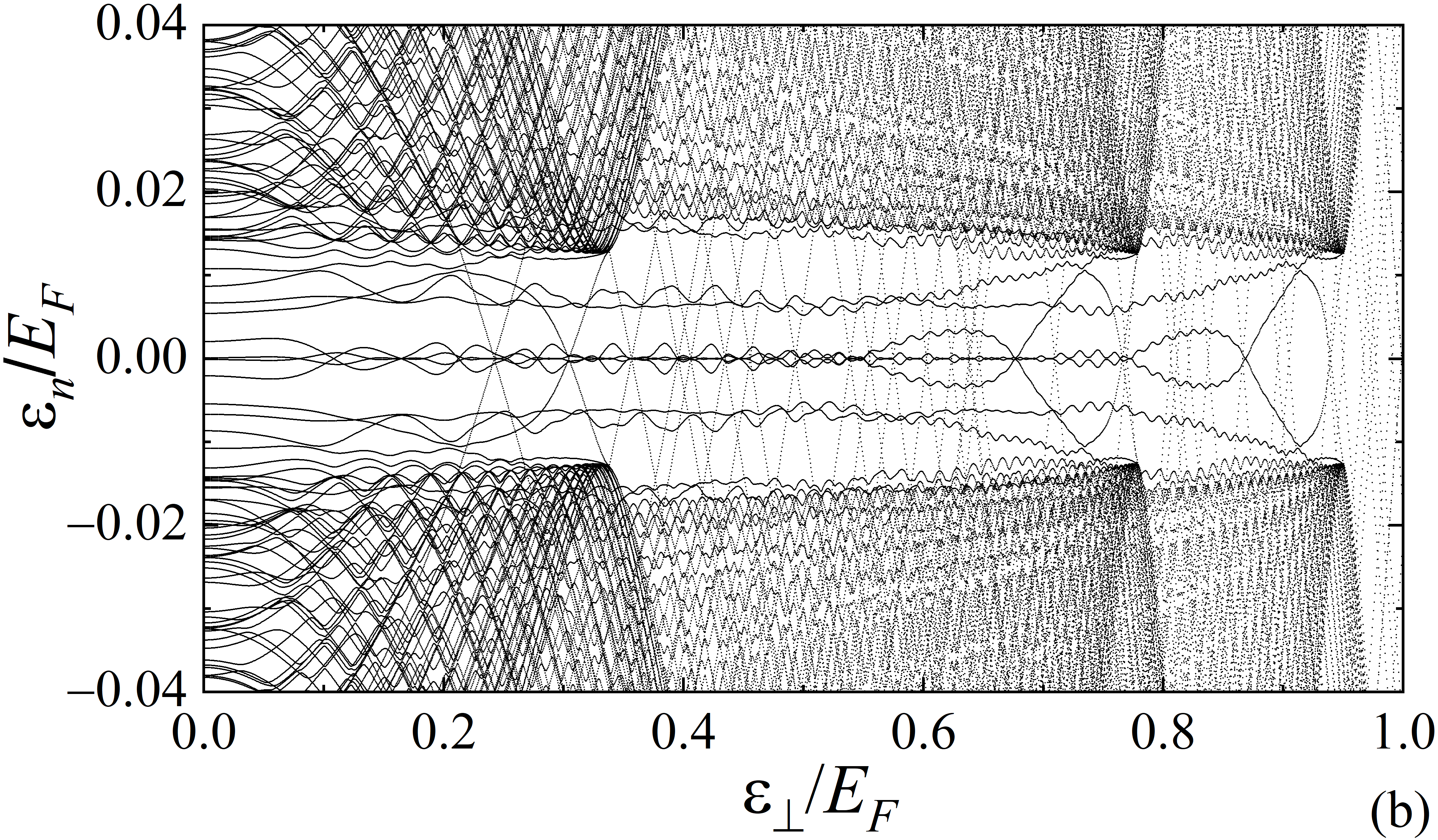
Figure 6: Energy spectra as a function of the transverse single particle energy $\varepsilon_{\perp}\equiv k_{x}^{2}/(2m)$. Two type of materials are considered for the central $\rm F$ region:(a) a nonmangetic normal metal with $h/E_{F}=0$, and (b) a fully spin-polarized ferromagnet, $h/E_{F}=1$. The macroscopic phase difference is fixed at $\Delta\varphi=0$. The magnitude of the exchange field in the outer two magnets have $h_{1,3}/E_{F}=0.1$. A narrow junction width is considered, with $W=10$.

Turning now to the electronic spectra, we present in Fig. 6 the quasiparticle energies $\varepsilon_{n}$, normalized by $E_{F}$, versus the normalized transverse energy $\varepsilon_{\perp}/E_{F}$. We consider two extreme values of the exchange field in the central junction region: Fig. 6(a) corresponds to a normal metal with $h_{2}/E_{F}=0$, and Fig. 6(b) contains the spectra for the half-metal case $h_{2}/E_{F}=1$. For a homogeneous bulk superconductor, a continuum of states occupy energies that fall outside of the bulk gap $\Delta_{0}$. For our system that includes multiple junction layers and quantum size-effects there will be substantial modifications to the scattering states and an emergence of discrete bound states in the excitation spectrum that approximately fall within the scaled gap $\Delta_{0}/E_{F}=2/(\pi k_{F}\xi_{0})$, corresponding to $\Delta_{0}/E_{F}\approx 0.0127$. Indeed as Fig. 6(a) shows, the eigenenergies $\varepsilon_{n}$ exhibit an intricate oscillatory behavior within the bulk gap region, although with limited quasiparticle excitations with energies near zero. This is in stark contrast to the half-metallic case in Fig. 6(b), where there are a considerable number of states that reside at zero energy. These results are consistent with the zero-energy peaks in the DOS profiles seen in Figs. 5(a,d).

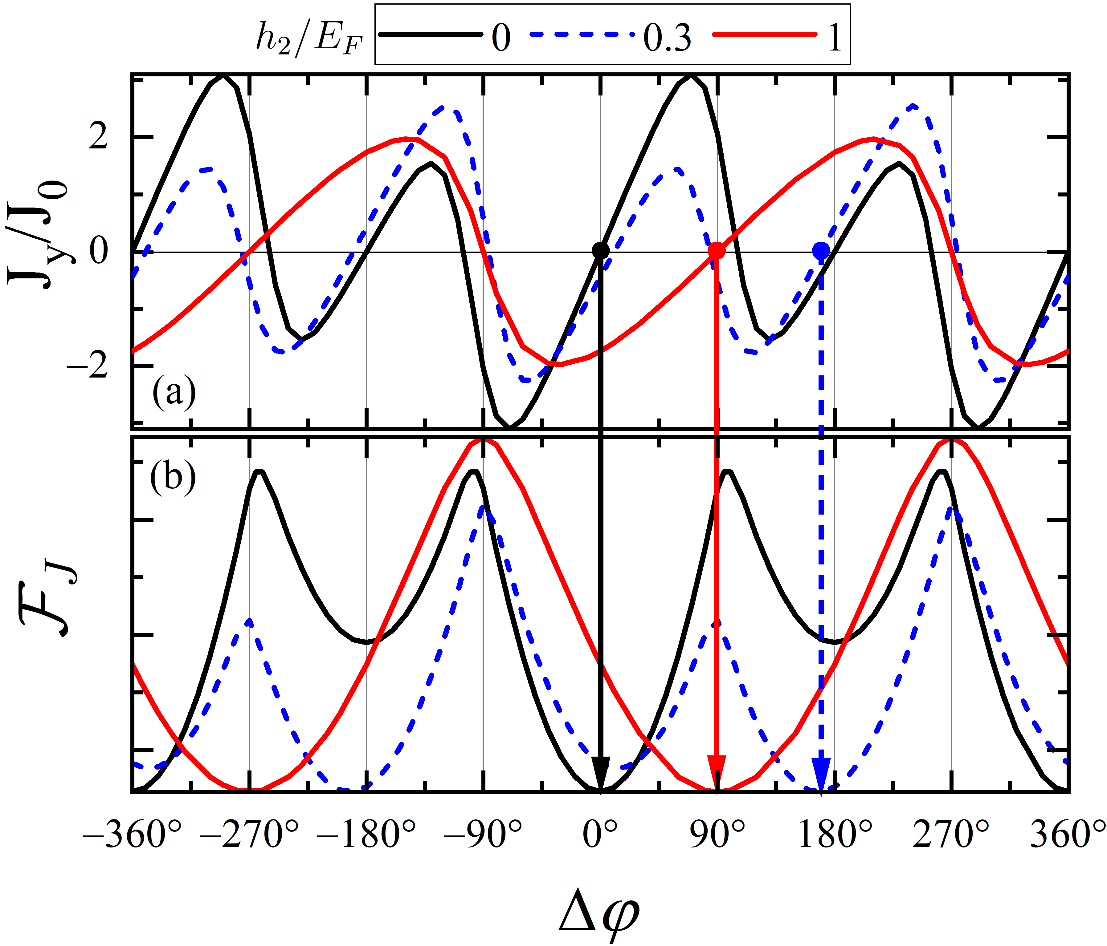
Figure 7: In (a) the current phase relations for different exchange fields of the central ferromagnet layer ${\rm F}_{2}$ are shown. A range of normalized exchange fields are considered (see legend), ranging from nonmagnetic ($h_{2}/E_{F}=0$) to half-metallic ($h_{2}/E_{F}=1$). The exchange fields for the outer two magnets are fixed at $h_{1}=h_{3}=0.1E_{F}$ and the $xyz$ configuration is considered. A narrow junction width is considered, with $W=10$. In (b) the free energy ${\cal F}_{J}$ is shown in arbitrary units over the same $\Delta\varphi$ in (a). The minima of each curve are shifted to the same level for clarity. The arrows identify the phase differences that correspond to the ground states of the systems in (a), with only the ground states for positive $\Delta\varphi$ shown.

Based on the findings of the DOS and energy spectra, it is clear that the exchange field in the central ferromagnet plays a crucial role in the formation of zero-energy modes and the existence of a spontaneous supercurrent. From the quasiparticle energy diagrams discussed above [Fig. 6], both the bound state and continuum state spectra shown contribute to the total supercurrent flow. We show in Fig. 7(a) how the supercurrent flow is modified by changes to the magnetic strength in the $\rm F_{2}$ region by presenting the current-phase relations for three representative values of $h_{2}/E_{F}$ (as labeled). It is evident that in going from $h_{2}/E_{F}=0$ to $h_{2}/E_{F}=1$, new harmonics emerge, and the $2\pi$ periodic CPR changes considerably, due in part to the proximity-induced long-ranged spin-polarized triplet correlations. In Fig. 7(a), the zero-phase state for $h_{2}/E_{F}=0$, exhibits no zero-phase supercurrent, since in this case there are only two orthogonal magnetizations present. Increasing the normalized exchange field up to 0.3 results in the emergence and gradual increase in the supercurrent when $\Delta\varphi=0$. In Fig. 7(b), stronger magnets are considered, with scaled values ranging from $0.4-1$. The largest jump in the anomalous current occurs when $h_{2}/E_{F}$ goes from $0.4$ to $0.6$, with subsequent increases giving smaller supercurrent increments. In particular, when $h_{2}/E_{F}$ increases to the half-metallic state from $h_{2}/E_{F}=0.8$, the anomalous current saturates, and further increases effect little change. The same trends are observed for the maximal supercurrent flow, not just the zero-phase current. Thus, the spontaneous supercurrent ramps up as the magnetization strength of middle ferromagnet increases.

When analyzing the CPR of finite-sized Josephson junctions, and determining the ground state of the system, it is useful to study the free energy, ${\cal F}$, which is comprised of two terms: ${\cal F}\equiv{\cal F}_{J}+{\cal F}_{\Delta}$. Here we define ${\cal F}_{\Delta}=\int dydz|\Delta(y,z)|^{2}/g$, and,

$${\cal F}_{J}=-2T\sum_{n}\ln\left[2\cosh\left(\frac{\epsilon_{n}}{2T}\right)\right].$$ (34)

For the cases considered in this paper, where $\partial{\cal F}_{\Delta}/\partial\Delta\varphi$ is small, we found that the contribution from ${\cal F}_{J}$ is sufficient to determine the ground state of the system. In Fig. 7(b), we therefore present ${\cal F}_{J}$ as a function of $\Delta\varphi$ for the same system parameters used in Fig. 7(a). The vertical arrows identify the ground states of each of the three CPRs, which always occur at zero current. It is important to note that the ground state phase difference $\varphi_{0}$ can vary from 0 to approximately $180^{\circ}$ by changing the strength of the ferromagnet in the central layer. In particular, by increasing $h_{2}/E_{F}$, the ground state shifts to higher phase differences. The next notable feature is that with the emergence of a $\varphi_{0}$ state, the CPR in Fig. 7(a) for $h_{2}/E_{F}=0.3$ is seen to exhibit a clear diode effect, whereby the supercurrent exhibits the following property: $|\sin(+\Delta\varphi+\varphi_{0})|\neq|\sin(-\Delta\varphi+\varphi_{0})|$. Thus, by appropriately tuning the phase difference between the superconductor banks, the dissipationless current flow can be made to have a one-way flow. This has practical applications as a nanoscale spintronics device with low energy consumption.

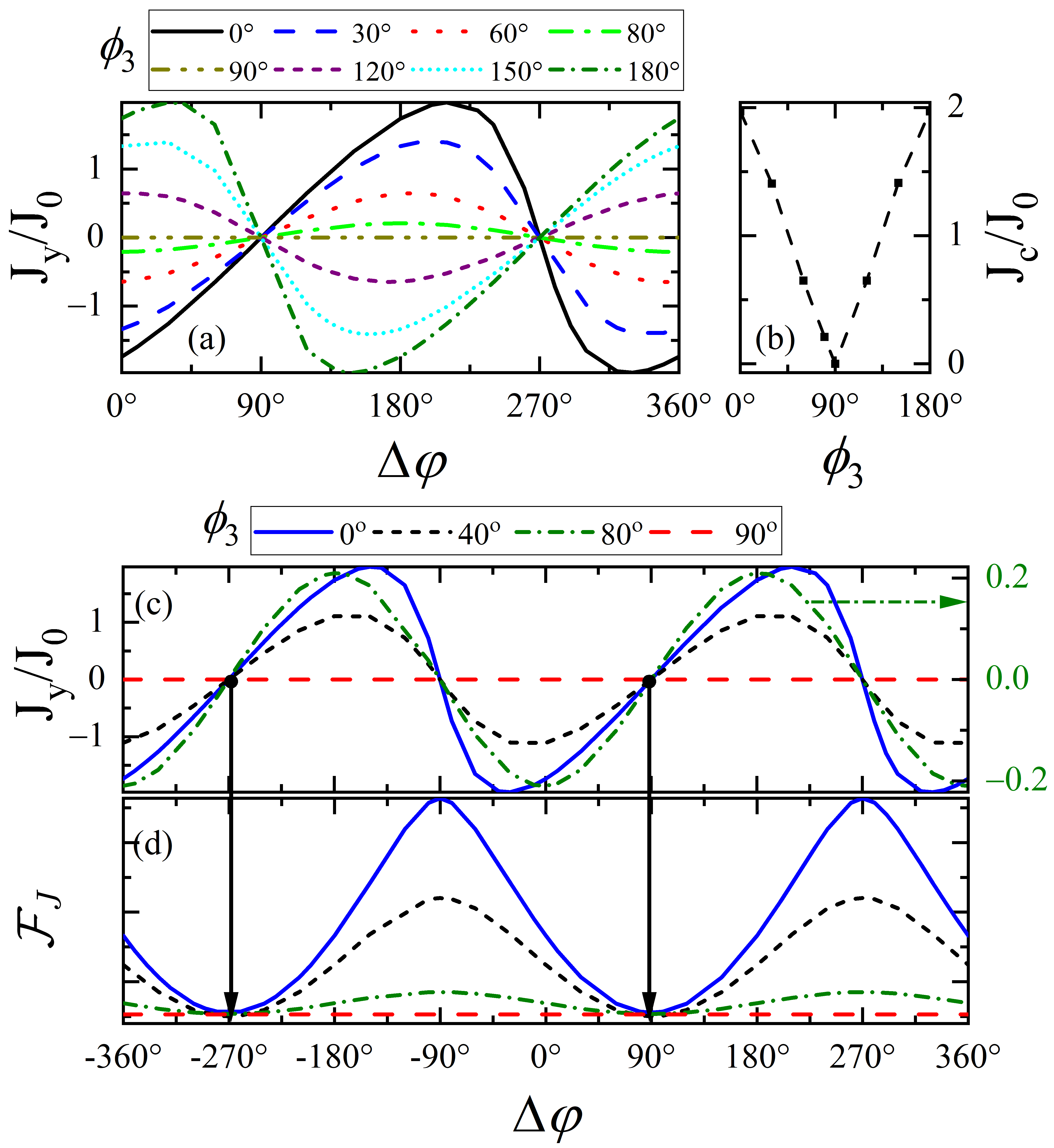
Figure 8: Top row: (a) Current phase relations for several magnetization angles $\phi_{3}$ (shown in the legend). (b) The corresponding critical current as a function of $\phi_{3}$ for the system in panel (a). In (c) an expanded view of the current phase relations is shown. A different scale for the $\phi_{3}=80^{\circ}$ case (labeled on the right vertical axis) is used to illustrate how the CPR evolves to a simple sine curve. The bottom panel (d) shows the free energy ${\cal F}_{J}$, with the vertical arrows identifying the ground state of the system. In all cases a half-metallic junction is considered with $h_{2}/E_{F}=1$, and the normalized exchange field in the outer two magnets is fixed at $h_{1}/E_{F}=h_{3}/E_{F}=0.1$, with the magnetizations along $x$ and $z$ directions, respectively. Results shown are for a narrow junction width of $W=10$.

Next, the effects of rotating the magnetization on the supercurrent are investigated, and we address the effectiveness of exchange-field rotations in controlling charge flow, including on/off switching of the supercurrent. Controlling the magnetization rotation can be achieved experimentally via, e.g., the application of external magnetic fields [77]. The orientation of the exchange field vector ${\bm{h}}_{3}$ is described by the two angles $\theta_{3}$ and $\phi_{3}$ [Eq. (15)]. Here we fix $\theta_{3}$ so that $\theta_{3}=90^{\circ}$, and variations in $\phi_{3}$ occur solely in the $y$-$z$ plane. In Fig. 8(a), the CPR is shown for several angles $\phi_{3}$ in the outer magnet (see legend). As $\phi_{3}$ varies from $\phi_{3}=0^{\circ}$ to $\phi_{3}=180^{\circ}$, the vector ${\bm{h}}_{3}$ goes from the $z$ direction to the $-z$ direction. The exchange field directions in the first and second ferromagnets remain fixed along the $x$ and $y$ directions, respectively. Here the $\rm F_{2}$ layer has a set exchange field of $h_{2}/E_{F}=1$. As the rotation angle increases, starting from $\phi_{3}=0^{\circ}$, the oscillation amplitudes in the CPR diminish until vanishing completely at $\phi_{3}=90^{\circ}$, at which point the exchange field in ${\rm F}_{3}$ is aligned with the central ferromagnet. Further increases in $\phi_{3}\geq 90^{\circ}$ results in a full reversal of the supercurrent with the CPR profile changing sign and mirroring the results for $\Delta\varphi\leq 90^{\circ}$ about the center line $\Delta\varphi=180^{\circ}$. Rotating the exchange field angle, $\phi_{3}$, can be achieved through external means, and thus the resultant control of the charge currents may be beneficial in practical devices, including nonvolatile memory elements. The experimentally relevant critical current $J_{c}$ as a function of $\phi_{3}$ is shown in Fig. 8(b), where the data is extracted from the CPR in Fig. 8(a). The critical supercurrent is calculated by finding the maximum of the supercurrent over the entire phase difference interval, i.e., $J_{c}=\max[J_{y}(\Delta\varphi)]$. The results show that if the outer ferromagnet $\rm F_{3}$ has its exchange field vector initially pointing along $\hat{\bm{y}}$ ($\phi_{3}=90^{\circ}$), then variations in $\phi_{3}$ about this point lead to an immediate linear increase in the critical current. In Fig. 8(c), the CPR for a select $\phi_{3}$ are shown over an expanded range of phase differences from $-360^{\circ}\leq\Delta\varphi\leq 360^{\circ}$. The scale on the right vertical axes corresponds to the $\phi_{3}=80^{\circ}$ case, which is seen to exhibit the conventional profile described by a sine function. To compliment the current-phase relations, Fig. 8(d) contains the free energies ${\cal F}_{J}$ for the curves in Fig. 8(c). As was found in Fig. 7, the ground state for $h_{2}/E_{F}=1$ corresponds to $\varphi_{0}=90^{\circ},-270^{\circ}$. Thus, while rotating the magnetization in the outer ferromagnet can result in the supercurrent changing sign or vanishing altogether, the $\varphi_{0}$ ground state is robust and remains unchanged.

Next, we investigate how other orientations of the exchange field vectors affect the zero-phase supercurrent response. In Fig. 9(a), the normalized supercurrent is shown as a function of the angles $\theta_{i}$ ($i=1,2,3$). In most cases above, the exchange fields in $\rm F_{1}$, $\rm F_{2}$, and $\rm F_{3}$ were in the $xyz$ configuration, respectively. Now, when a given angle, e.g., $\theta_{2}$ is varied, $\rm F_{1}$ and $\rm F_{3}$ keep their exchange field vectors fixed along the $x$ and $z$ directions, respectively. When $\theta_{1}$ is varied, $\phi_{1}$ is set to $\phi_{1}=0^{\circ}$, so $\theta_{1}$ sweeps occur in the $x$-$z$ plane. Thus when rotating from $\theta_{1}=0^{\circ}$, to $\theta_{1}=90^{\circ}$, ${\bm{h}}_{1}$ goes from being aligned along the $x$ direction, to along the $z$ direction, respectively. This creates a situation with the two outer ferromagnets are both aligned along the $z$ direction, destroying the magnetic inhomogeneity needed for a finite anomalous current to flow, as observed in Fig. 9(a). As seen, the peak zero-phase current does not occur for the $xyz$ configuration as one might expect, but rather when the exchange field vector in $\rm F_{1}$ is slightly skewed between the $x$ and $z$ directions. When $\theta_{2}$ is now varying, the outer magnets are fixed according to ${\bm{h}}_{1}=h_{1}\hat{\bm{x}}$, and ${\bm{h}}_{3}=h_{3}\hat{\bm{z}}$. When $\theta_{2}$ is zero (or a multiple of $\pi$), the leftmost two ferromagnets have colinear exchange fields, and thus the zero-phase current is zero in those instances, as seen. As the exchange field rotates in the half-metal, it is observed that $|J_{y}(\Delta\varphi=0)|$ is largest when $\theta_{2}=\pi/2,3\pi/2$, i.e., precisely when the exchange field is strictly along $\pm y$. Similar behavior is observed when $\theta_{3}$ varies, with the main difference being an offset of the peak amplitude of the zero-phase current. Thus, for the outer magnets their optimal zero-phase supercurrent flow occurs when their exchange field vectors point between the $x$ and $z$ directions. Considering now magnetization rotations in the $y$-$z$ plane, we present in Fig. 9(b) the zero-phase current as a function of the angular variables $\phi_{2}$ and $\phi_{3}$. In each case, we fix $\theta_{2,3}=90^{\circ}$. As $\phi_{2}$ or $\phi_{3}$ varies from $0^{\circ}$ to $180^{\circ}$, the corresponding exchange fields change their alignment from along $z$ to along $y$, respectively. Therefore, we find that for the rotations of the exchange field vector in the $y$-$z$ plane (see Fig. 1), plane, when $|J_{y}(\Delta\varphi)|$ is maximal for certain angles $\phi_{2}$, it is zero when $\phi_{3}$ equals those angles. More specifically, the curves have identical profiles that are offset from one another by $90^{\circ}$.

The CPR and free energy diagrams are illustrated in Fig. 9(c) and Fig. 9(d) respectively. A range of orientations $\theta_{3}$ are considered, as shown in the legend. The ${\rm F}_{1}$ and ${\rm F}_{2}$ magnets have their exchange fields aligned along the $x$ and $y$ directions, respectively. For each $\theta_{3}$ shown, $\phi_{3}=0^{\circ}$ is fixed, so that $\theta_{3}$ variations result in ${\bm{h}}_{3}$ rotating in the $x$-$z$ plane. For $\theta_{3}=0^{\circ}$, the exchange field vector in ${\rm F}_{3}$ is pointing along $x$, while $\theta_{3}=90^{\circ}$, has it along the $z$ direction. The CPR in Fig. 9(c) shows that it retains its profile as ${\bm{h}}_{3}$ rotates, and simply undergoes an overall shift by an amount that is proportional to $\theta_{3}$. The free energy ${\cal F}_{J}$ has the same behavior as Fig. 9(d) shows, changing $\theta_{3}$ causes the ground state phase difference $\varphi_{0}$ to shift similarly. This tunablilty of the ground state by magnetization rotations can be achieved through an external magnetic field, or a spin torque mechanism.

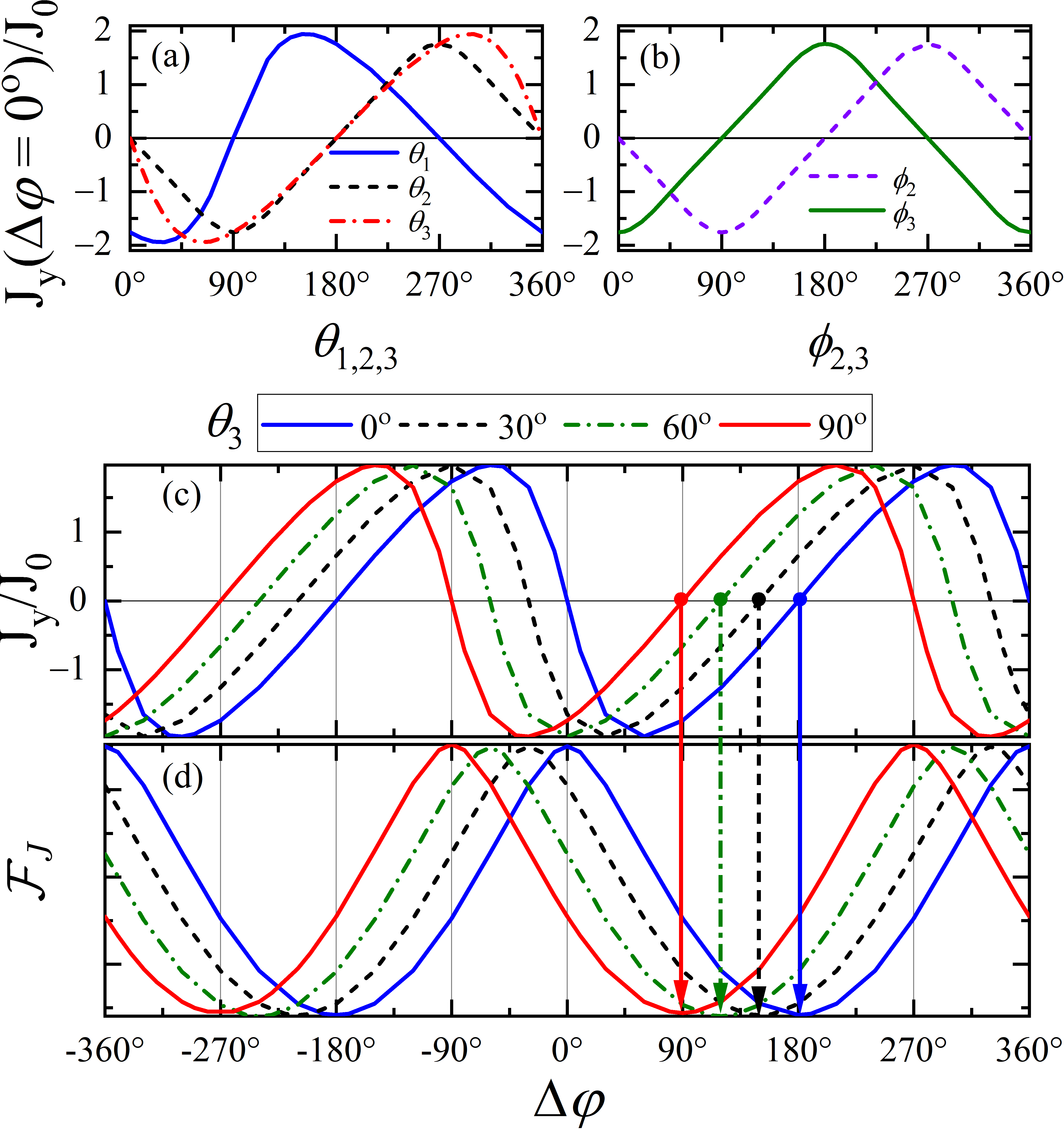
Figure 9: The top row (a) and (b) illustrate the normalized anomalous supercurrent $J_{y}(\Delta\varphi=0^{\circ})$ as a function of the angles $\theta_{1,2,3}$ and $\phi_{1,2}$ describing the exchange field vector orientations in the respective ferromagnets ${\rm F}_{1,2,3}$. In (c) the normalized Josephson current is shown as a function of phase difference $\Delta\varphi$ for the selected angles $\theta_{3}=0^{\circ},\theta_{3}=30^{\circ},\theta_{3}=60^{\circ},\theta_{3}=90^{\circ}$. The corresponding ground states are depicted by arrows pointing towards the free-energy minima in (d).

We now explore the spin currents that arise when there is a zero phase difference between the superconducting electrodes and a finite supercurrent. The anomalous supercurrent that is generated can become spin-polarized when passing through the ferromagnetic trilayer. In Figs. 10(a-c), the spin currents flowing in the $y$ direction $S_{y\sigma}$ are shown for each spin $\sigma$. All spin currents are plotted as functions of the dimensionless coordinate $Y$, with $Z=W/2$ fixed. In Fig. 10(d) the spin current for the $z$ component of spin, flowing in the transverse $z$ direction $S_{zz}$ is shown. The legend identifies the different angles of rotation $\phi_{3}$ of the exchange field vector ${\bm{h}}_{3}$. The Josephson junction has ${\bm{h}}_{1}$ and ${\bm{h}}_{2}$ in the trilayer oriented along the $x$ and $y$ directions, respectively. For the type of magnetic arrangement studied here, the components of the spin current tensor $S_{zx}$ and $S_{zy}$ are zero. As seen in Fig. 10(a), the $x$ component of spin has its current magnitude largest at the interface between $\rm F_{2}$ and $\rm F_{3}$ (the vertical line at $Y=210$) for $\phi_{3}=0^{\circ},180^{\circ}$. This corresponds to the magnetic configurations where the exchange field vectors in the magnets are each orthogonal to one another. For all other $0^{\circ}<\phi_{3}<180^{\circ}$, the magnitude of the spin current reduces, including vanishing at $\phi_{3}=90^{\circ}$. Similar trends are observed in Fig. 10(b) for the $y$ projection of spin, with now a reduction in the overall magnitude of the spin currents. Additionally, we find that $|S_{yy}|$ increases approximately linearly in the thin outer magnets, before entering the half-metal, where it modulates slightly while levelling out. For both Figs. 10(a) and 10(b), the spin currents vanish when $\phi_{3}=90^{\circ}$, which for this orientation, corresponds to when the anomalous current is zero. For the $z$ component of spin, the magnitude of the spin current peaks at the interface between $\rm F_{1}$ and $\rm F_{2}$ ($Z=160$). Unlike what was observed in Fig. 10(a), the spin current is insensitive to changes in $\phi_{3}$. A transverse spin current also flows, as shown in Fig. 10(d), where the $z$ component of the spin current flowing in the $z$ direction, $S_{zz}$, is shown. Within the left superconductor ($Y<150$), there is a weakly decaying spin current that oscillates upon entering the adjacent ferromagnet and then $|S_{zz}|$ increases rapidly near the interface (at $Y=160$) separating the ferromagnet from the half-metal. Within the half-metal and ferromagnet $\rm F_{3}$ ($160<Y<220$), the spin current is relatively constant (aside from a slight modulation at the interface). Finally within the second superconductor ($Y>220$), the spin current again undergoes a slow decay that depends on the particular angle $\phi_{3}$.

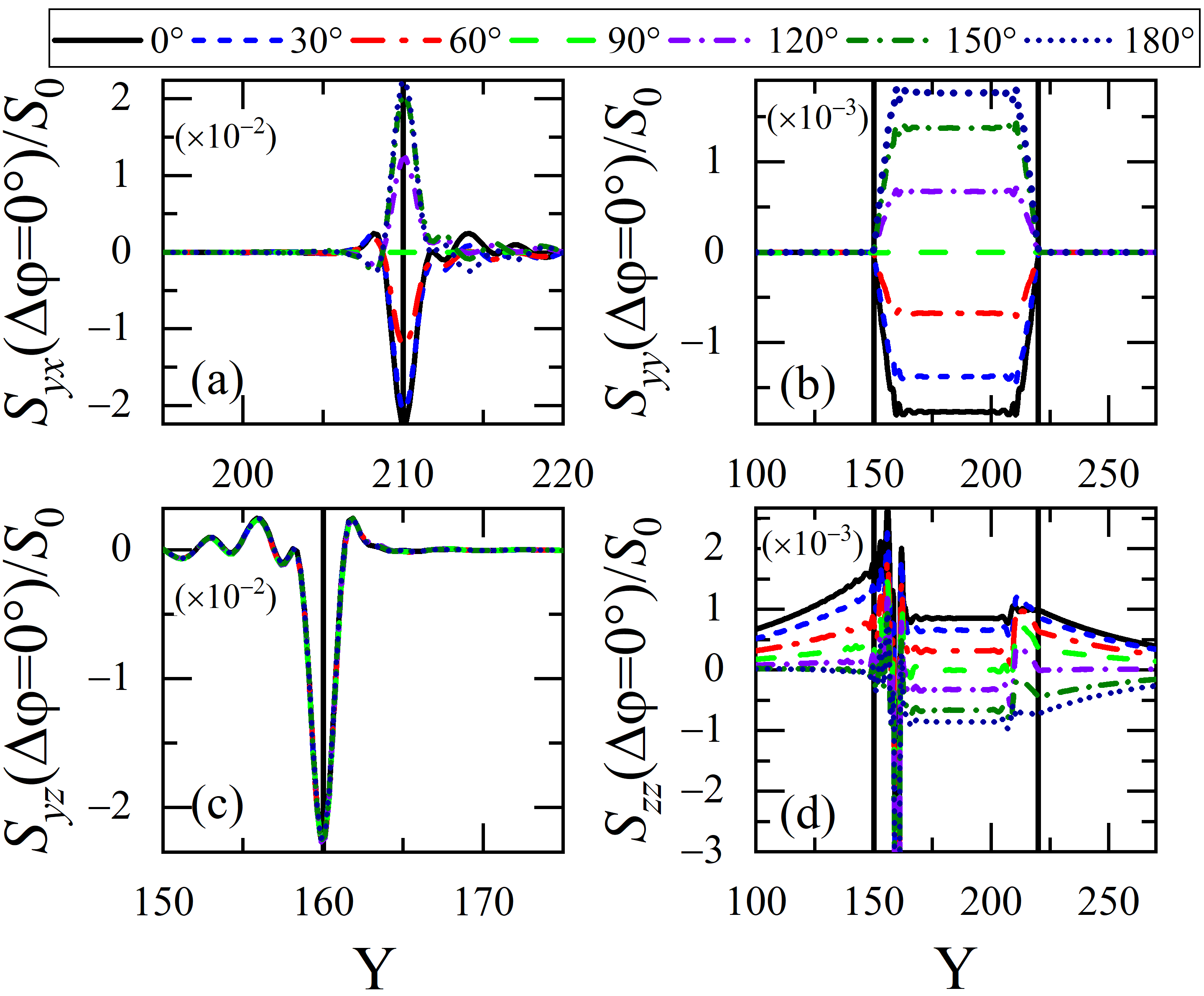
Figure 10: The nonzero components of the spin current tensor are shown as a function of the normalized coordinate $Y=k_{F}y$. The phase difference between the two superconducting banks is set to $\Delta\varphi=0$. The central ferromagnet is a half metal ($h_{2}/E_{F}=1$), while the outer ferromagnets of the trilayer are fixed at $h_{1}/E_{F}=h_{3}/E_{F}=0.1$. The exchange field vector ${\bm{h}}_{3}$ is allowed to vary in $y$-$z$ plane (the legend gives the rotation angle $\phi_{3}$). The vertical lines denote ferromagnet interfaces.

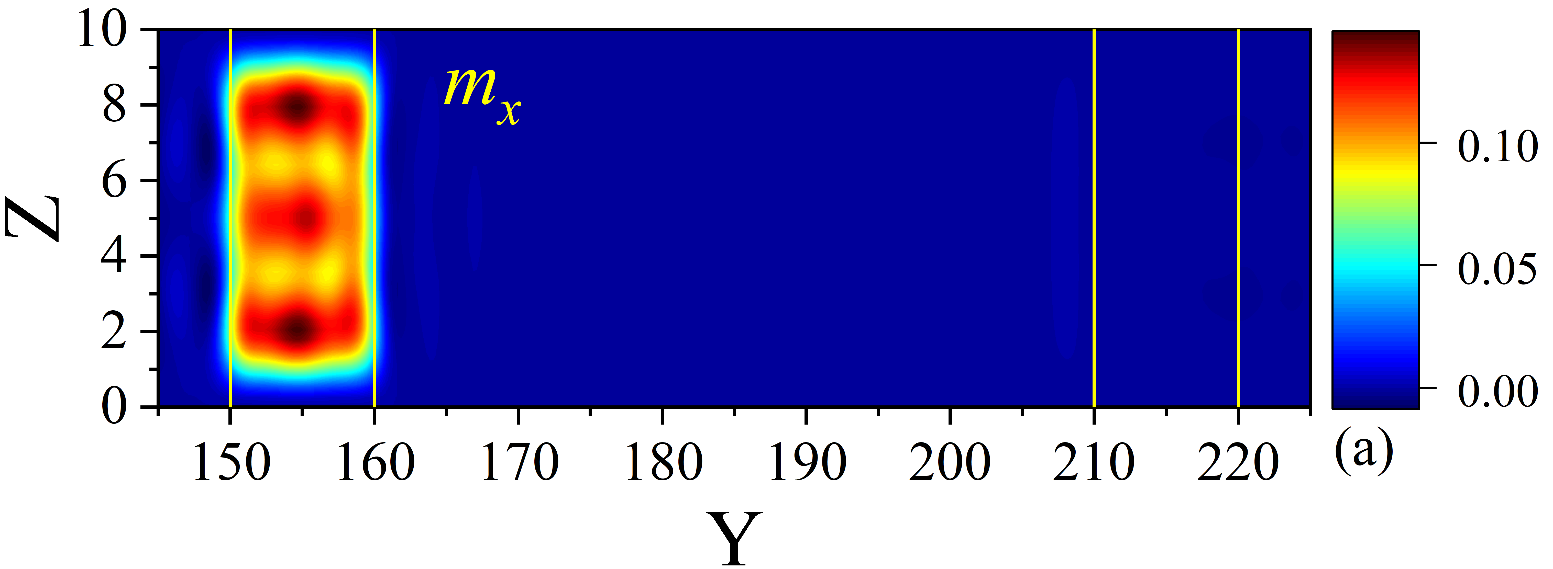
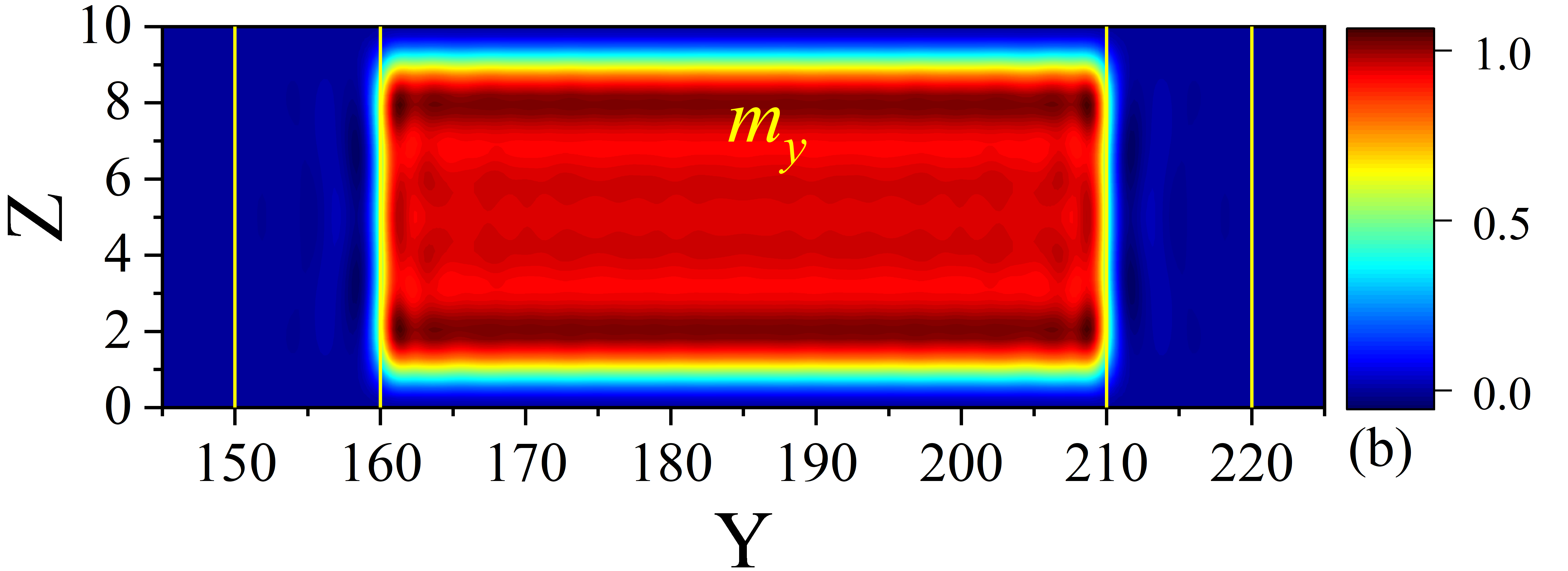
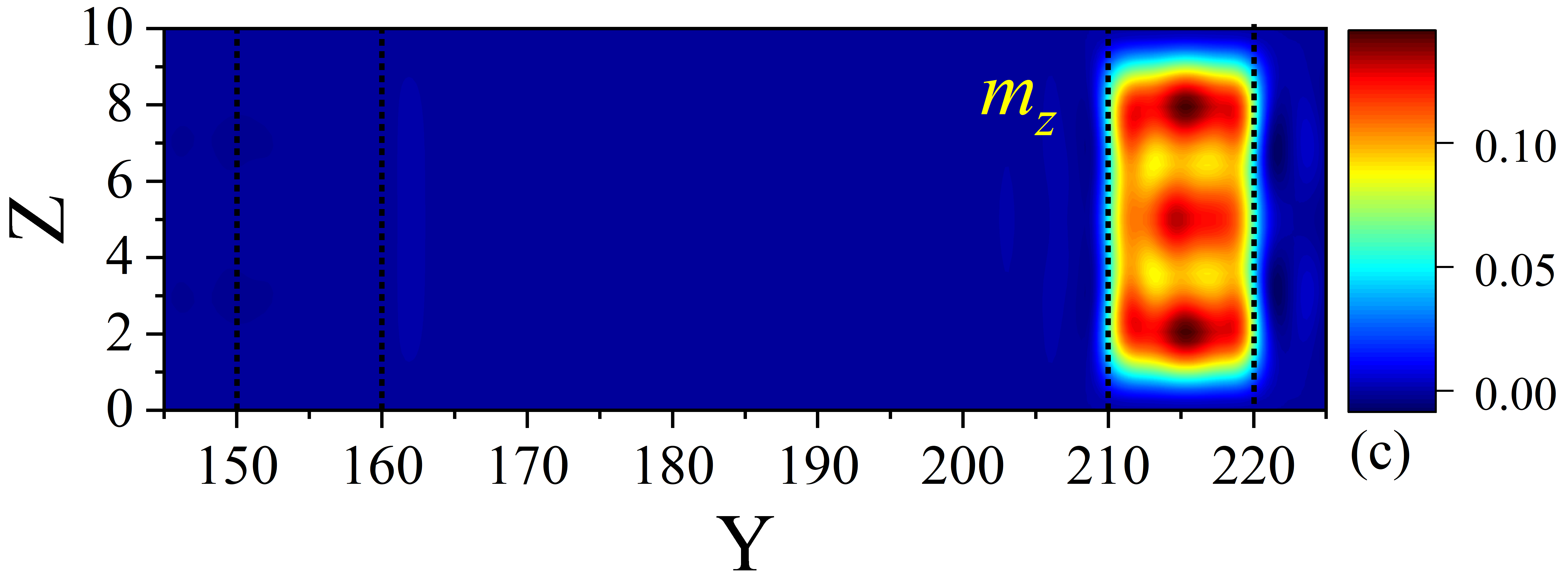
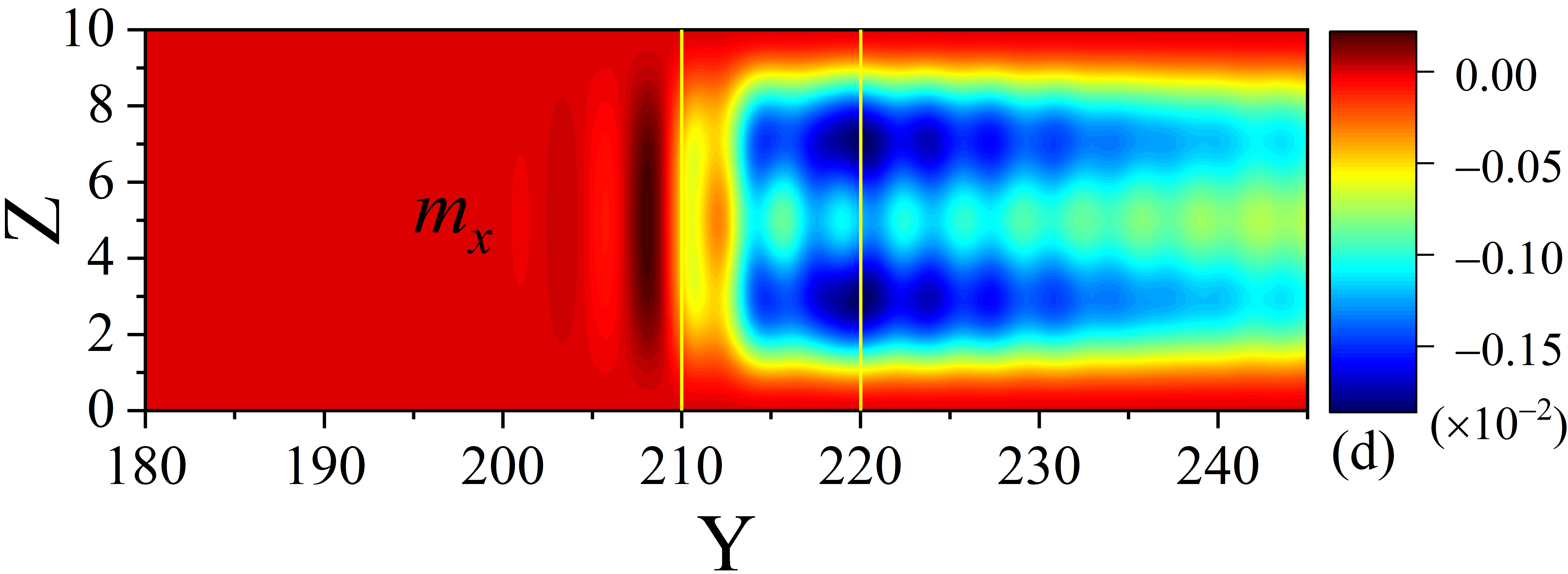
Figure 11: The components of magnetic moment are shown (as labeled) as a function of the dimensionless coordinates $Y$ and $Z$. Panel (d) shows $m_{x}$ from (a) over a different scale to illustrate the spin polarization that extends into $\rm F_{3}$ and the adjacent superconductor. The yellow vertical lines enclose the ferromagnet regions. The phase difference between the S banks is set to $\Delta\varphi=0^{\circ}$, and we consider the $xyz$ configuration for the magnets.

In discussing spin transport quantities, we expect that the presence of an anomalous supercurrent and proximity effects due to the exchange interactions, will lead to a spin torque transfer and a corresponding leakage of magnetism. The interaction of the spin current with the magnetization is also relevant for memory technologies, where the storage of information depends on the relative orientation of the magnetizations. In Fig. 11, a spatial mapping of each component of the magnetic moment is shown for a half-metallic Josephson junction with the exchange field vectors in the $xyz$ configuration. The phase difference $\Delta\varphi$ is set to zero, so that an anomalous supercurrent is generated. The thin outer magnets have $h_{1,3}/E_{F}=0.1$. In Fig. 11(a), the $x$ component of magnetic moment $m_{x}$ (normalized by $\mu_{B}n_{e}$) is shown. As seen, $m_{x}$ is confined mainly to the $\rm F_{1}$ region ($150<Y<160$), vanishing in the vicinity of the hard wall boundaries at $Z=0$ and $Z=10$. Due to the mutual proximity effects between the surrounding superconductor and half-metal, there is also a leakage of magnetization into those regions, as well as an increase in $m_{x}$ from its bulk values within $\rm F_{1}$. The same behavior is also observed in Fig. 11(c) for the $z$ component of magnetic moment. The half metal region exhibits a more uniform magnetic moment [Fig. 11(b)], but also exhibits similar proximity effects, including rapid variations near the top and bottom of the structure, as well as an enhancement of its spin polarization near the edges at $Z=2$ and $Z=8$. We also present in Fig. 11(d) $m_{x}$ over a different scale, to demonstrate the typical long-ranged spin-imbalance that occurs, which in this case originates from $\rm F_{1}$ and is transferred into $\rm F_{3}$ ($210<Y<220$) and the adjacent superconductor ($Y>220$).

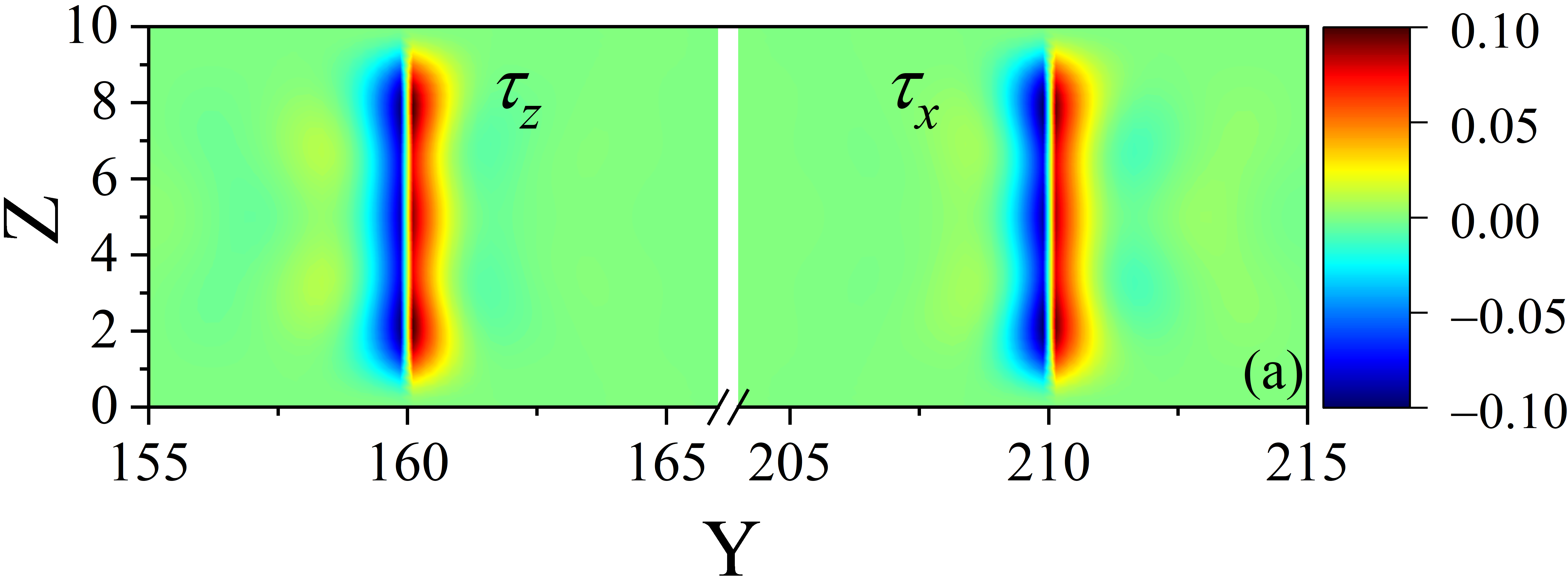
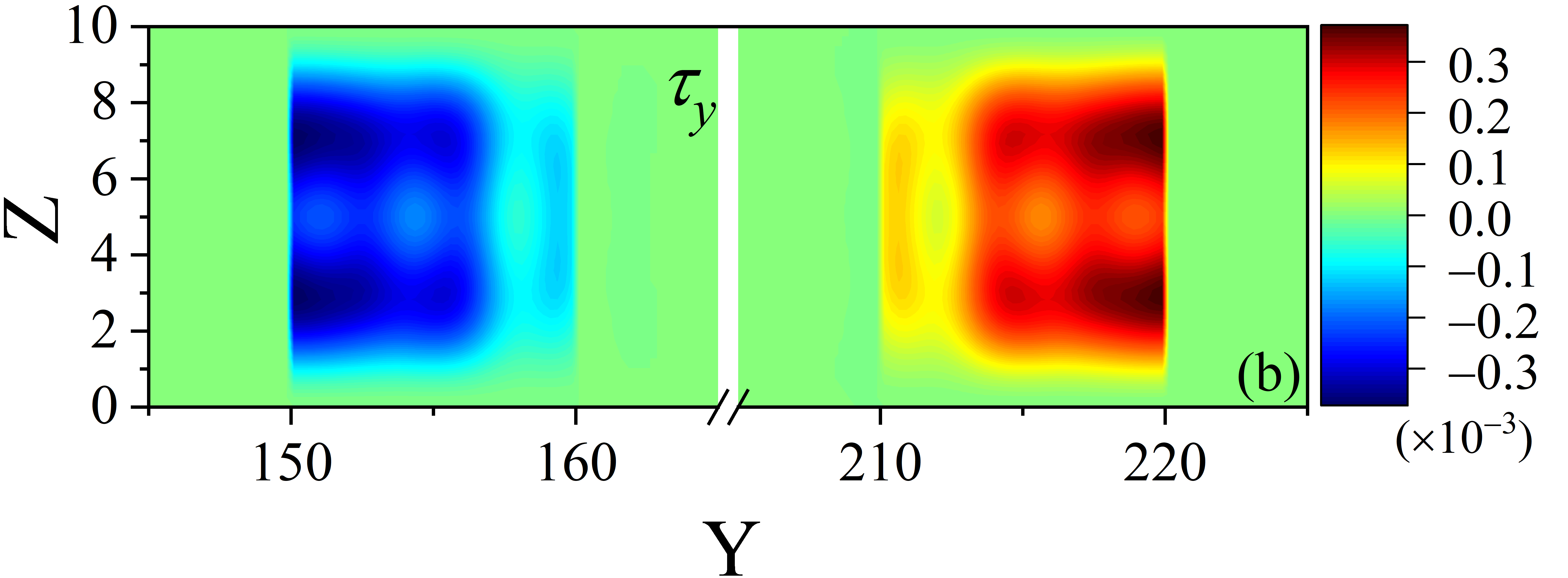
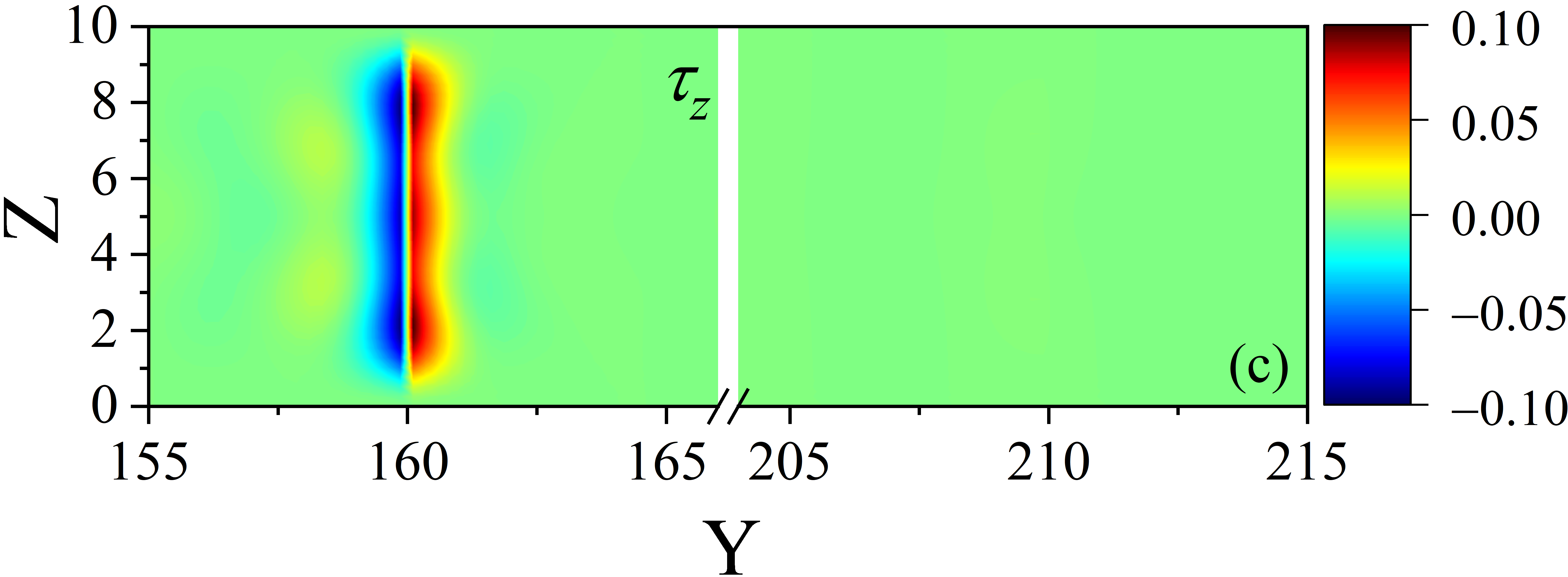
Figure 12: Spatial mapping of the $x$, $y$, and $z$ components of the spin torque. The phase difference between the two superconducting banks is set to $\Delta\varphi=0$, which established a zero-phase supercurrent. The central ferromagnet is a half metal ($h_{2}/E_{F}=1$), while the outer ferromagnets of the trilayer are fixed at $h_{1}/E_{F}=h_{3}/E_{F}=0.1$. Here we fix $\theta_{3}$ so that $\theta_{3}=90^{\circ}$, and variations in $\phi_{3}$ occur solely in the $y$-$z$ plane. In (a) and (b), $\phi_{3}=0^{\circ}$, and in (c), $\phi_{3}=90^{\circ}$. For panel (c), $\tau_{z}$ is the only nonzero component.

The spatial behavior of the spin currents discussed in relation to Fig. 10 can be modified by the local magnetizations due to the spin-exchange interaction, via the mechanism of spin torque transfer. The use of STT in half-metallic Josephson junctions can result in faster magnetization switching times in random access memories. The STT effect has been widely found to occur in a broad variety of ferromagnetic materials, including half-metals, making it widely accessible experimentally [78]. It is thus important not only to understand the behavior of the spin-polarized currents in ferromagnetic Josephson junctions, but also the various ways in which to manipulate them for practical spintronics type of devices. We therefore investigate in Fig. 12 the equilibrium spin torques throughout the junction regions as functions of the normalized coordinates $Y$ and $Z$. We calculate ${\bm{\tau}}$ from the magnetization and prescribed exchange fields [24] via:

$${\bm{\tau}}=-\frac{2}{\mu_{B}}{\bm{m}}\times{\bm{h}}.$$ (35)

In Figs. 12(a) and 12(b), the outer free magnetization angle is set to $\phi_{3}=0^{\circ}$ (the $xyz$ configuration) so that an anomalous supercurrent is generated. In Fig. 12(c), $\phi_{3}=90^{\circ}$ (the $xyy$ configuration), and hence no self-biased supercurrent is present. Beginning with the top row, Fig. 12(a), the two spin torque components $\tau_{x}$ and $\tau_{z}$ are shown superimposed on the same density plot. The half metal boundaries are clearly seen at $Y=160$ and $Y=210$. It is observed that the STT is most pronounced near these boundaries, peaking antisymmetrically on each side. This behavior is consistent with the spin currents shown in Fig. 10 and the expressions in Eq. (33), where for weak spatial variations in the $z$ direction, Eq. (33) states that $\tau_{x}=\partial S_{yx}/\partial y$ and $\tau_{z}=\partial S_{yz}/\partial y$. Therefore the slope of the curves in Fig. 10(a,c) gives a good approximation for $\tau_{x}$ and $\tau_{z}$ directly. In particular, the normalized $S_{yx}$ in Fig. 10(a) exhibits a slope that undergoes an abrupt sign change when crossing the interface at $Y=210$, where the slope is zero, in agreement with the sign change of $\tau_{x}$ about the interface [see in Fig. 12(a)]. The same analysis shows consistency between Fig. 12(b) and $\tau_{z}$, with the notable feature that changing the angle $\phi_{3}$ in the free layer has no effect on the $z$ component of the spin currents flowing in the $y$ direction. From Eq. (30), we see that $\bm{\tau}$ is responsible for the change in local magnetizations due to the flow of spin-polarized currents. In Fig. 12(b), the weaker $y$ component of the spin torque is shown. Unlike the other two components in Fig. 12(a), $\tau_{y}$ resides solely in the two outer magnets $\rm F_{1}$ and $\rm F_{3}$. This follows from the leakage of magnetism discussed in relation to Fig. 11(d), where the $x$ component of the magnetization in $\rm F_{1}$ extends all the way to $\rm F_{3}$ via the spin currents $S_{yy}$ in Fig. 10(b). It should be emphasized that for there to be a $y$ component of spin torque in $\rm F_{3}$, there must also be a finite $m_{x}$ there since $\tau_{y}$ in $\rm F_{3}$ is proportional to $h_{z}m_{x}$. Finally, we illustrate in Fig. 12(c) the $z$ component of the spin torque for the rotation angle $\phi_{3}=90^{\circ}$. For this magnetic configuration, the anomalous current vanishes [See Fig. 8(c)]. As seen in Fig. 10, all spin currents flowing in the $y$ direction also vanish, except for those with a $z$ spin projection [Fig. 10(c)], which do not depend on $\phi_{3}$. Since $\tau_{z}\approx\partial S_{yz}/\partial y$, the torque in Fig. 12(c) is centered on the $\rm F_{1}/F_{2}$ interface at $Y=160$.

IV Conclusions

Motivated by recent advances and interest in making use of half-metallic materials (supporting one spin species) in superconducting hybrid structures, we have studied the spatial mappings and superconducting phase dependency of the charge supercurrents, spin supercurrents, spin torques, and density of states in ballistic SF₁F₂F₃S Josephson configurations where the magnetizations in the F layers can have arbitrary directions and strengths. To this end, we have generalized a wavefunction approach, incorporating efficient computational techniques for optimizing the diagonalization of large-size matrices in a parallel computing environment. This allows our method to properly account for realistic three-dimensional systems, including planar SF₁F₂F₃S hybrids where the system is confined in two dimensions, and the third dimension is considered to be infinite. Interestingly, the charge supercurrent as a function of magnetization strength in the $\rm F_{2}$ layer shows that the critical supercurrent reaches its maximum value at high values close to the half-metallic phase so that it becomes only slightly different from its F₁N F₃ counterparts. In a situation where the magnetization in the three F layers are mutually orthogonal (the ”$xyz$” configuration), we find that a self-biased spontaneous supercurrent exists, which is largest when the $\rm F_{2}$ layer is a half-metal. We study the behavior of the spontaneous supercurrent for various magnetization orientations in the F layers and determine the most favorable configurations. We find that for intermediate exchange field strengths of the central ferromagnet layer, a superconducting diode effect emerges, whereby a unidrectional dissipationless current can flow by appropriately tuning the phase gradient between the outer superconductor electrodes. The DOS studies illustrate robust zero energy peaks in the $xyz$ configuration that disappears when there is no three orthogonal magnetization components in the system. The zero energy peaks are spatially located in the $\rm F_{1}$ and $\rm F_{3}$ layers and become largest when $\rm F_{3}$ is a half-metal. Further studies on the spatial distributions of other important physical quantities demonstrate an extremely long-ranged magnetic moment and spin currents extending from one superconductor in the SF₁F₂F₃S system to the other. This long-ranged behavior and anomalous supercurrent flow generated spin torques controllable by rotations of the magnetization in the outer ferromagnet.

Apart from the results obtained for the specific SF₁F₂F₃S system in the half-metallic regime, this generalized approach can be further expanded to systems with spin-orbit coupling, various types of impurities, and an external magnetic field. Unlike the limitations that the quasiclassical method demands, our approach can cover systems far beyond the quasiclassical approximations and properly account for band curvatures and arbitrary ratios among the energy scales, such as the exchange field and chemical potential, found in many types of systems.

Appendix A Numerical method

When expanding the quasiparticle amplitudes $u_{n,\sigma}$, and $v_{n,\sigma}$ in terms of a complete set of basis functions [see Eq. (16)], for numerical purposes the sums are cut off at [79, 80] $N_{l}{\sim}k_{F}l/\pi\sqrt{1+\max\{h_{1},h_{2},h_{3}\}}$, and $N_{w}{\sim}k_{F}w/\pi\sqrt{1+\max\{h_{1},h_{2},h_{3}\}}$, thus ensuring that all of the quantum states are included over the wide range of energy scales present in the problem. Inserting Eqs. (16) into the matrix eigensystem (Eq. (14)) and invoking the orthogonality of the basis functions, we get the following set of matrix elements:

$$[{\cal H}_{0}]_{pqp^{\prime}q^{\prime}} =\langle pq|H_{0}|p^{\prime}q^{\prime}\rangle=\frac{4}{wl}\int_{0}^{l}\int_{0}^{w}dzdy\sin\Big{(}\frac{p\pi y}{l}\Big{)}\sin\Big{(}\frac{q\pi z}{w}\Big{)}\left[-\frac{1}{2m}\Big{(}\frac{\partial^{2}}{\partial z^{2}}+\frac{\partial^{2}}{\partial y^{2}}\Big{)}+\frac{1}{2m}k_{x}^{2}-\mu\right]\sin\Big{(}\frac{p^{\prime}\pi y}{l}\Big{)}\sin\Big{(}\frac{q^{\prime}\pi z}{w}\Big{)},$$

$$+\frac{4}{wl}\int_{0}^{l}\int_{0}^{w}dzdy\sin\Big{(}\frac{p\pi y}{l}\Big{)}\sin\Big{(}\frac{q\pi z}{w}\Big{)}U(y,z)\sin\Big{(}\frac{p^{\prime}\pi y}{l}\Big{)}\sin\Big{(}\frac{q^{\prime}\pi z}{w}\Big{)},$$ (36)

$$[{\cal D}]_{pqp^{\prime}q^{\prime}} =\langle pq|\Delta|p^{\prime}q^{\prime}\rangle=\frac{4}{wl}\int_{d_{N}}^{l}\int_{0}^{w}dzdy\sin\Big{(}\frac{p\pi y}{l}\Big{)}\sin\Big{(}\frac{q\pi z}{w}\Big{)}\Delta(y,z)\sin\Big{(}\frac{p^{\prime}\pi y}{l}\Big{)}\sin\Big{(}\frac{q^{\prime}\pi z}{w}\Big{)},$$ (37)

$$[{\cal I}_{j}]_{pqp^{\prime}q^{\prime}} =\langle pq|h_{j}|p^{\prime}q^{\prime}\rangle=\frac{4}{wl}\int_{d_{S}}^{d_{S}+d_{F1}}\int_{0}^{w}dzdy\sin\Big{(}\frac{p\pi y}{l}\Big{)}\sin\Big{(}\frac{q\pi z}{w}\Big{)}h_{j1}\sin\Big{(}\frac{p^{\prime}\pi y}{l}\Big{)}\sin\Big{(}\frac{q^{\prime}\pi z}{w}\Big{)}$$

$$+\frac{4}{wl}\int_{d_{S}+d_{F1}}^{d_{S}+d_{F1}+d_{F2}}\int_{0}^{w}dzdy\sin\Big{(}\frac{p\pi y}{l}\Big{)}\sin\Big{(}\frac{q\pi z}{w}\Big{)}h_{j2}\sin\Big{(}\frac{p^{\prime}\pi y}{l}\Big{)}\sin\Big{(}\frac{q^{\prime}\pi z}{w}\Big{)}$$ (38)

$$+\frac{4}{wl}\int_{d_{S}+d_{F1}+d_{F2}}^{d_{S}+d_{F1}+d_{F2}+d_{F3}}\int_{0}^{w}dzdy\sin\Big{(}\frac{p\pi y}{l}\Big{)}\sin\Big{(}\frac{q\pi z}{w}\Big{)}h_{j3}\sin\Big{(}\frac{p^{\prime}\pi y}{l}\Big{)}\sin\Big{(}\frac{q^{\prime}\pi z}{w}\Big{)},\quad j=x,y,z,$$

where $q,q^{\prime},p,p^{\prime}$ are integers. In what follows, we scale the expressions in Eqs. (36-A) by the Fermi energy $E_{F}$ to make them dimensionless. The integrations for the free-particle term in Eq. (36) are easily done, which after dividing each term by the Fermi energy $E_{F}=k_{F}^{2}/(2m)$, takes the following dimensionless form:

$$[{\cal H}_{0}]_{pqp^{\prime}q^{\prime}}=\left[\left\{\left(\frac{p\pi}{k_{F}l}\right)^{2}+\left(\frac{q\pi}{k_{F}w}\right)^{2}\right\}+\frac{\varepsilon_{\perp}}{E_{F}}-1\right]\delta_{qq^{\prime}}\delta_{pp^{\prime}}.$$ (39)

Here, for simplicity, the scattering potential $U(y,z)$ is assumed to be zero in this work. The above dependence on four indices $q,q^{\prime},p,p^{\prime}$ can be reduced to a system of two indices $k$ and $k^{\prime}$ suitable for matrix operations by changing the index operations so that, $\{p,q\}\rightarrow k$, and $\{p^{\prime},q^{\prime}\}\rightarrow k^{\prime}$. This creates a more manageable and compact system of equations

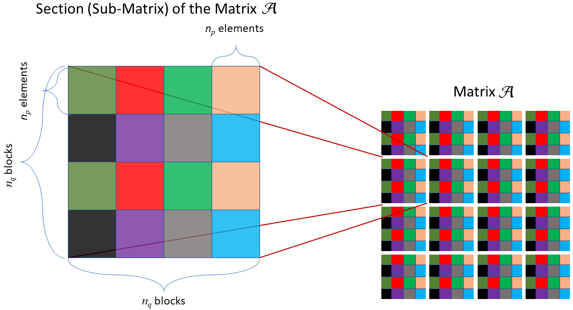
Figure 13: A representative case of the distributed memory approach where one matrix is comprised of 16 sections. Each matrix is distributed within its block cyclic distribution scheme. The image shows one of the 16 sections distributed over 2 processor row and 4 processor columns. For large problems, the number of processor rows and columns for each grid could be significant.

We can now cast the matrix eigensystem in Eq. (14) into a following form suitable for numerical purposes: ${\cal A}\Psi_{n}=\epsilon_{n}\Psi_{n}$, where the matrix ${\cal A}$ is given by,

$${\cal A}= \begin{pmatrix}{\cal H}_{0}-{\cal I}_{z}&-{\cal I}_{x}+i{\cal I}_{y}&0&{\cal D}\\[5.0pt] -{\cal I}_{x}-i{\cal I}_{y}&{\cal H}_{0}+{\cal I}_{z}&{\cal D}&0\\[5.0pt] 0&{\cal D}^{*}&-({\cal H}_{0}-{\cal I}_{z})&-{\cal I}_{x}-i{\cal I}_{y}\\[5.0pt] {\cal D}^{*}&0&-{\cal I}_{x}+i{\cal I}_{y}&-({\cal H}_{0}+{\cal I}_{z})\end{pmatrix},$$ (40)

Here $\overline{\epsilon}_{n}=\epsilon_{n}/E_{F}$, and the expansion coefficients are written in vector form: $\Psi_{n}=({\bm{u}}_{n,\uparrow},{\bm{u}}_{n,\downarrow},{\bm{v}}_{n,\uparrow},{\bm{v}}_{n,\downarrow})^{T}$, with ${\bm{u}}_{n,\sigma}=(u_{n,\sigma}^{1},\cdots,u_{n,\sigma}^{N})^{T}$, and ${\bm{v}}_{n,\sigma}=(v_{n,\sigma}^{1},\cdots,v_{n,\sigma}^{N})^{T}$. The rank of the matrix in Eq. (40) is $N=4N_{l}N_{w}$. The numerical implementation of the solver used in solving the $4N\times 4N$ eigensystem in Eq. (40) was done using object-oriented Fortran with the MPI [81], OpenMP [82], and ScaLAPACK [83] libraries.

The energy $\varepsilon_{\perp}$ corresponds to the kinetic energy of the quasiparticles that are moving transverse to the longitudinal $x$ direction. This parameter is effectively a good quantum number and when performing the sum over states for a given physical quantity, a fixed number $n_{\varepsilon_{\perp}}$ of these transverse states must be included. During each step of the solution process, and for the final calculations, the eigenvectors and eigenenergies for $n_{\varepsilon_{\perp}}$ matrices need to be calculated. Each of these $n_{\varepsilon_{\perp}}$ matrices are distributed in a block cyclic manner onto a subset of the available MPI ranks called a processor grid (PG). Due to the construction of the problem, the matrix ${\cal A}$ can be split into 16 equally sized sections, each containing one or many PGs, depending on the $n_{\rm row}\times n_{\rm col}$ form of a PG for a given problem. A diagram representing this distributed memory process is shown in Fig. 13. Each section is made of $n_{q}\times n_{q}$ blocks and each block contains $n_{p}\times n_{p}$ matrix elements. Each one of these sections must be perfectly tessellated by the block size, which then allows individual ranks to own the same block in each section of the matrix ${\cal A}$. This allows for reduced computational and communication complexity.

For communication, MPI ranks are grouped into four communicators, which are graphically represented in Fig. 14. These four are: MPI_COMM_WORLD, a communicator for the PG (Grid communicator), a communicator for the specific column within the PG (local column communicator), and a communicator with the corresponding grid rank in all of the other processor grids (Rank communicator). At the end of every iteration, all system properties of interest within the solver are summed using MPI collectives across one, some or all of the communicator groups depending on the particular requirements for a given property.

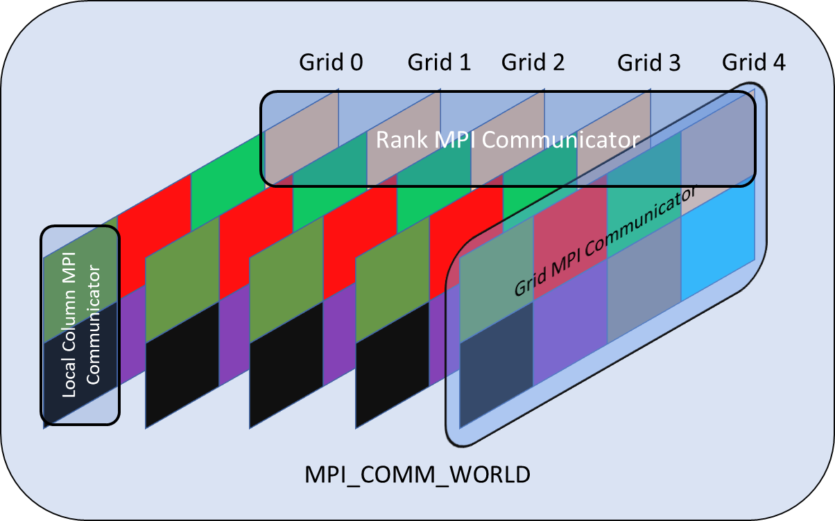
Figure 14: MPI_COMM_WORLD is partitioned into multiple processor grids. Each rank within the program uses 4 separate communicators at different times. MPI_COMM_WORLD, a communicator for the PG (Grid communicator), a communicator for the specific column within the processor grid (local column communicator), and a communicator with the corresponding grid rank in all of the other processor grids (Rank communicator).

Appendix B Optimizations and Computational Techniques

In addition to parallelization via MPI, thread-level parallelization was implemented using OpenMP. A naïve coding for the calculation of $u_{n,\sigma}(y,z)$, and $v_{n,\sigma}(y,z)$ would require a loop over $q$, within a loop over $p$, within a loop over $z$, and finally within a loop over $y$ for 4 levels of looping. The quasiparticle expansions in Eq. (16) that involve the terms, $\sum_{p}u_{n,\sigma}^{p,q}\sin(p\pi y/l)$ and $\sum_{p}v_{n,\sigma}^{p,q}\sin(p\pi y/l)$, could be calculated and stored within a vector for every $q$ within each iteration of the loop over $y$, outside of the loop over $z$. This reduces the number of nested loops required. In addition, inner loops were written to be of the form: c = sum(a(:) $\cdot$ b(:)), making it possible to fully exploit vector-based compiler optimizations.

Appendix C Memory requirements

Figure 15: Matrix Rank and Minimum Total Memory Requirements. Growth of the rank of matrix ${\cal A}$ and associated required memory to calculate the eigenvectors of a representative matrix. Here, $W=100$, blocking is set to $n_{p}$, and cluster size=1. The grey curve is the required memory to solve the eigenvectors for one matrix. The orange curve is the associated memory requirement on each process, with the grid size listed adjacent to each point.

The memory requirements for the problem can be categorized in three major categories: the matrix ${\cal A}$, its eigenvectors, and the workspace required by ScaLAPACK to calculate the eigenvectors. The memory required for ${\cal A}$ and its associated eigenvectors is equivalent and scales as $\alpha(4n_{p}n_{q})^{2}$. Calculations were performed using 32-bit precision, so the value of $\alpha$ is 8 bytes (4 bytes each for the real and imaginary portions). The amount of workspace required by ScaLAPACK was dependent upon the rank of $\cal{A}$, with the number of rows and columns being held by that specific process, and a clustersize parameter (additional memory to orthogonalize eigenvectors). Due to library constraints, the number of 4-byte elements in the ScaLAPACK work array was limited to $2^{31}$, or 8 GB. This was a per-process limit on just the work array, and each rank could use more than 8 GB total. Furthermore, more than one process could be launched on a single compute node to make efficient use of available resources.

The growth of the memory requirements is shown in Fig. 15, using nominal values for the system parameters. The width of the junction was kept constant, and its normalized length was increased from 115 to 1215 in increments of 100. As can be seen, the total required memory for a single matrix increases with the square of the matrix rank. By increasing the number of processes used to evaluate ${\cal A}$, the per-process memory could be kept roughly level. The per-process memory usage and grid size is selected by maximizing the amount of memory managed by a single process.

References

- [1] L. R. Tagirov, M. Yu. Kupriyanov, V. N. Kushnir, and A. Sidorenko, Superconducting Triplet Proximity and Josephson Spin Valves, Functional Nanostructures and Metamaterials for Superconducting Spintronics. NanoScience and Technology. Springer, Cham (2018).
- [2] L.R. Tagirov, Low-field superconducting spin switch based on a superconductor/ferromagnet multilayer, Phys. Rev. Lett., 83, 2058 (1999).
- [3] V.T. Petrashov, I.A. Sosnin, I. Cox, A. Parsons, C. Troadec, Giant mutual proximity effects in ferromagnetic/superconducting nanostructures, Phys. Rev. Lett. 83, 3281 (1999).
- [4] V. V. Ryazanov, V. A. Oboznov, A. V. Veretennikov, and A. Yu. Rusanov, Intrinsically frustrated superconducting array of superconductor-ferromagnet-superconductor junctions, Phys. Rev. B 65, 020501(R) (2001).
- [5] A. Kadigrobov, R. I. Shekhter, and M. Jonson, Quantum Spin Fluctuations as a Source of Long-Range Proximity Effects in Diffusive Ferromagnet-Superconductor Structures, Europhys. Lett. 54, 394 (2001).
- [6] G. Deutscher, F. Meunier, Coupling between ferromagnetic layers through a superconductor, Phys. Rev. Lett. 22, 395 (1969).
- [7] S. Oh, D. Youm, and M. R. Beasley, A superconductive magnetoresistive memory element using controlled exchange interaction, Appl. Phys. Lett. 71, 2376 (1997).
- [8] Y.V. Fominov, A.A. Golubov, M.Y. Kupriyanov, Triplet proximity effect in FSF trilayers, JETP Lett., 77, 510 (2003).
- [9] J. Zhu, I.N. Krivorotov, K. Halterman, O.T. Valls, Angular dependence of the superconducting transition temperature in ferromagnet-superconductor-ferromagnet trilayers, Phys. Rev. Lett. 105, 207002 (2010).
- [10] J. Y. Gu, C.-Y. You, J. S. Jiang, J. Pearson, Ya. B. Bazaliy, and S. D. Bader, Magnetization-Orientation Dependence of the Superconducting Transition Temperature in the Ferromagnet-Superconductor-Ferromagnet System: CuNi/Nb/CuNi, Phys. Rev. Lett., 89, 267001 (2002).
- [11] M. Alidoust, and K. Halterman, Proximity Induced Vortices and Long-Range Triplet Supercurrents in Ferromagnetic Josephson Junctions and Spin Valves, J. Appl. Phys. 117, 123906 (2015).
- [12] Ya. V. Fominov, A. A. Golubov, T. Yu. Karminskaya, M. Yu. Kupriyanov, R. G. Deminov, L. R. Tagirov, Superconducting triplet spin valve, JETP Letters 91, 308 (2010).
- [13] P. V. Leksin, N. N. Garif’yanov, I. A. Garifullin, Ya. V. Fominov, J. Schumann, Y. Krupskaya, V. Kataev, O. G. Schmidt, and B. Büchner, Evidence for triplet superconductivity in a superconductor-ferromagnet spin valve, Phys. Rev. Lett. 109, 057005 (2012).
- [14] M. Avdeev, Y. Proshin, The Solitary Superconductivity in Dirty FFS Trilayer with Arbitrary Interfaces, J. Low Temp. 185, 453 (2016).
- [15] V.I. Zdravkov, J. Kehrle, G. Obermeier, D. Lenk, H.-A. Krug von Nidda, C. Müller, M. Yu. Kupriyanov, A.S. Sidorenko, S. Horn, R. Tidecks, L.R. Tagirov, Experimental observation of the triplet spin-valve effect in a superconductor-ferromagnet heterostructure, Phys. Rev. B 87, 144507 (2013).
- [16] E. Antropov, M. S. Kalenkov, J. Kehrle, V.I. Zdravkov, R. Morari, A. Socrovisciuc, D. Lenk, S. Horn, L.R. Tagirov, A. D. Zaikin, A.S. Sidorenko, H. Hahn, R. Tidecks, Experimental and theoretical analysis of the upper critical field in ferromagnet–superconductor–ferromagnet trilayers, Supercond. Sci. Technol. 26, 085003 (2013).
- [17] Y.N. Khaydukov, G.A. Ovsyannikov, A.E. Sheyerman, K.Y. Constantinian, L. Mustafa, T. Keller, M.A. Uribe-Laverde, Yu.V. Kislinskii, A.V. Shadrin, A. Kalabukhov, B. Keimer, D. Winkler, Evidence for spin-triplet superconducting correlations in metal-oxide heterostructures with noncollinear magnetization, Phys. Rev. B 90, 035130 (2014).
- [18] T. Vezin, C. Shen, J. E. Han, and I. Zutic, Enhanced spin-triplet pairing in magnetic junctions with s-wave superconductors, Phys. Rev. B 101, 014515 (2020).
- [19] A.I. Buzdin, L.N. Bulaevskii, and S.V. Panyukov, Critical-current oscillations as a function of the exchange field and thickness of the ferromagnetic metal (F) in an S-F-S Josephson junction, Pis’ma Zh. Eksp. Teor. Fiz. 35, 147 (1982) [JETP Lett. 35, 178 (1982)].
- [20] A.I. Buzdin, Proximity effects in superconductor-ferromagnet heterostructures, Rev. Mod. Phys. 77, 935 (2005).
- [21] F. S. Bergeret, A. F. Volkov, and K. B. Efetov, Odd triplet superconductivity and related phenomena in superconductor-ferromagnet structures, Rev. Mod. Phys. 77, 1321 (2005).
- [22] R.S. Keizer, S.T.B. Goennenwein, T.M. Klapwijk, G. Miao, G. Xiao and A. Gupta, A spin triplet supercurrent through the half-metallic ferromagnet , Nature 439, 825 (2006).
- [23] T.S. Khaire, M.A. Khasawneh, W.P. Pratt Jr, N.O. Birge, Observation of spin-triplet superconductivity in Co-based Josephson junctions, Phys. Rev. Lett. 104, 137002 (2010).
- [24] K. Halterman, O. T. Valls, and C.-T. Wu, Charge and spin currents in ferromagnetic Josephson junctions, Phys. Rev. B 92, 174516 (2015).
- [25] M. Alidoust, K. Halterman, and O.T. Valls, Zero-Energy Peak and Triplet Correlations in Nanoscale SFF Spin-Valves, Phys. Rev. B 92, 014508 (2015).
- [26] M. Alidoust, A. Zyuzin, K. Halterman, Pure Odd-Frequency Superconductivity at the Cores of Proximity Vortices, Phys. Rev. B 95, 045115 (2017).
- [27] L. Kuerten, C. Richter, N. Mohanta, T. Kopp, A. Kampf, J. Mannhart, and H. Boschker, In-gap states in superconducting interfaces observed by tunneling spectroscopy, Phys. Rev. B 96, 014513 (2017).
- [28] K. Halterman and M. Alidoust, Induced energy gap in finite-sized superconductor/ferromagnet hybrids, Phys. Rev. B 98, 134510 (2018).
- [29] K. Halterman and M. Alidoust, Half-Metallic Superconducting Triplet Spin Valve, Phys. Rev. B 94, 064503 (2016).
- [30] M. Alidoust and K. Halterman, Half-Metallic Superconducting Triplet Spin Multivalve, Phys. Rev. B 97, 064517 (2018).
- [31] J. Coey and M. Venkatesan, Half-metallic ferromagnetism: Example of , J. of Appl. Phys. 91, 8345 (2002).
- [32] C. Visani, Z. Sefrioui, J. Tornos, C. Leon, J. Briatico, M. Bibes, A. Barthelemy, J. Santamaria, and J. E. Villegas, Equal-spin Andreev reflection and long-range coherent transport in high-temperature superconductor/half-metallic ferromagnet junctions, Nat. Phys. 8, 539 (2012).
- [33] Z. Sefrioui, D. Arias, V. Pena, J. E. Villegas, M. Varela, P.Prieto, C.Leon, J.L.Martinez, and J.Santamaria, Ferromagnetic/superconducting proximity effect in superlattices, Phys. Rev. B 67, 214511 (2003).
- [34] K. Dybko, K. Werner-Malento, P. Aleshkevych, M. Wojcik, M. Sawicki, and P. Przyslupski, Possible spin-triplet superconducting phase in the trilayer, Phys. Rev. B 80, 144504 (2009).
- [35] Y. Kalcheim, T. Kirzhner, G. Koren, and O. Millo, Long-range proximity effect in ferromagnet/superconductor bilayers: Evidence for induced triplet superconductivity in the ferromagnet, Phys. Rev. B 80, 144504 (2009).
- [36] A. Srivastava, L. A. B. Olde Olthof, A. Di Bernardo, S. Komori, M. Amado, C. Palomares-Garcia, M. Alidoust, K. Halterman, M. G. Blamire, J. W. A. Robinsonn, Magnetization-control and transfer of spin-polarized Cooper pairs into a half-metal manganite, Phys. Rev. Applied 8, 044008 (2017).
- [37] A. Singh, S. Voltan, K. Lahabi, and J. Aarts, Colossal Proximity Effect in a Superconducting Triplet Spin Valve Based on the Half-Metallic Ferromagnet , Phys. Rev. X 5, 021019 (2015).
- [38] S. Mironov and A. Buzdin, Triplet proximity effect in superconducting heterostructures with a half-metallic layer, Phys. Rev. B 92, 184506 (2015).
- [39] M. Alidoust, C. Shen, I. Zutic, Cubic spin-orbit coupling and anomalous Josephson effect in planar junctions, Phys. Rev. B 103, 060503 (2021).
- [40] H. Sickinger, A. Lipman, M. Weides, R. G. Mints, H. Kohlstedt, D. Koelle, R. Kleiner, and E. Goldobin, Experimental Evidence of a Josephson Junction, Phys. Rev. Lett. 109,107002 (2012).
- [41] A. Zyuzin, M. Alidoust, D. Loss, Josephson junction through a disordered topological insulator with helical magnetization, Phys. Rev. B 93, 214502 (2016).
- [42] I. V. Bobkova, A. M. Bobkov, A. A. Zyuzin, M. Alidoust, Magnetoelectrics in disordered topological insulator Josephson junctions, Phys. Rev. B 94, 134506 (2016).
- [43] M. Alidoust and H. Hamzehpour, Spontaneous supercurrent and phase shift parallel to magnetized topological insulator interfaces, Phys. Rev. B 96, 165422 (2017).
- [44] A. Assouline, C. Feuillet-Palma, N. Bergeal, T. Zhang, A. Mottaghizadeh, A. Zimmers, E. Lhuillier, M. Marangolo, M. Eddrief, P. Atkinson, M. Aprili, H. Aubin, Spin-Orbit induced phase-shift in Josephson junctions, Nat. Comm. 10, 126 (2019).
- [45] M. Alidoust, Self-biased current, magnetic interference response, and superconducting vortices in tilted Weyl semimetals with disorder, Phys. Rev. B 98, 245418 (2018).
- [46] M. Alidoust and K. Halterman, Evolution of pair correlation symmetries and supercurrent reversal in tilted Weyl semimetals, Phys. Rev. B 101, 035120 (2020).
- [47] K. Kulikov, D. Sinha, Yu. M. Shukrinov, and K. Sengupta, Josephson junctions of Weyl and multi-Weyl semimetals, Phys. Rev. B 101, 075110 (2020).
- [48] M. Alidoust, M. Willatzen, and A.-P. Jauho, Strain-engineered Majorana zero energy modes and Josephson state in black phosphorus, Phys. Rev. B 98, 085414 (2018).
- [49] M. Alidoust, M. Willatzen, and A.-P. Jauho, Fraunhofer response and supercurrent spin switching in black phosphorus with strain and disorder, Phys. Rev. B 98, 184505 (2018).
- [50] M. Alidoust, Critical supercurrent and state for probing a persistent spin helix, Phys. Rev. B 101, 155123 (2020).
- [51] J.F. Liu, K.S. Chan, Anomalous Josephson current through a ferromagnetic trilayer junction, Phys. Rev. B 82, 184533 (2010).
- [52] I. Margaris, V. Paltoglou, N. Flytzanis, Zero phase difference supercurrent in ferromagnetic Josephson junctions, J. Phys.:Condens Matter 22, 445701 (2010).
- [53] M.A. Silaev, I.V. Tokatly, F.S. Bergeret, Anomalous current in diffusive ferromagnetic Josephson junctions, Phys. Rev. B 95, 184508 (2017).
- [54] Zh. Devizorova and S. Mironov, Crossover between standard and inverse spin-valve effect in atomically thin superconductor/half-metal structures, Phys. Rev. B 100, 064519 (2019).
- [55] Zh. Devizorova, S. Mironov, and A. I. Buzdin, Effect of spin-triplet correlations on Josephson transport in atomically thin superconductor/half-metal/superconductor structures, Phys. Rev. B 103, 224510 (2021).
- [56] Z. Shomali, R. Asgari, Spin transfer torque and exchange coupling in Josephson junctions with ferromagnetic superconductor reservoirs, J. Phys.: Condens. Matter 32, 035806 (2020).
- [57] H. Meng, Y. Ren, J. E. Villegas, and A. I. Buzdin, Josephson current through a ferromagnetic bilayer: Beyond the quasiclassical approximation, Phys. Rev. B 100, 224514 (2019).
- [58] H. Ness, I. A. Sadovskyy, A. E. Antipov, M. van Schilfgaarde, R. M. Lutchyn, First principles supercurrent calculation in realistic magnetic Josephson junctions, arXiv:2101.10601.
- [59] M. Alidoust, and K. Halterman, Supergap and subgap enhanced currents in asymmetric Josephson junctions, Phys. Rev. B 102, 224504 (2020).
- [60] A. G. Golubov, M. Yu. Kupriyanov, and E. llichev, The current-phase relation in Josephson junctions, Rev. Mod. Phys. 76, 411 (2004).
- [61] A. A. Reynoso, G. Usaj, C. A. Balseiro, D. Feinberg, and M. Avignon, Anomalous Josephson current in junctions with spin polarizing quantum point contacts, Phys. Rev. Lett. 101, 107001 (2008).
- [62] A. I. Buzdin, Direct Coupling Between Magnetism and Superconducting Current in the Josephson Junction, Phys. Rev. Lett. 101, 107005 (2008).
- [63] D. B. Szombati, S. Nadj-Perge, D. Car, S. R. Plissard, E. P. A. M. Bakkers, and L. P. Kouwenhoven, Anomalous Josephson current through a Spin-Orbit coupled quantum dot, Nat. Phys. 3742 (2016).
- [64] N. Mohanta, S. Okamoto, E. Dagotto, Skyrmion control of Majorana states in planar Josephson junction, Commun. Phys. 4, 163 (2021).
- [65] H. Wu, Y. Wang, P. K. Sivakumar, C. Pasco, S. S. P. Parkin, Y.-J. Zeng, T. McQueen, M. N. Ali, Realization of the field-free Josephson diode, arXiv:2103.15809 (2021).
- [66] C. Baumgartner, L. Fuchs, A. Costa, S. Reinhardt, S. Gronin, G. C. Gardner, T. Lindemann, M. J. Manfra, P. E. Faria Junior, D. Kochan, J. Fabian, N. Paradiso, C. Strunk, A Josephson junction supercurrent diode, arXiv:2103.06984 (2021).
- [67] J. J. He, Y. Tanaka, N. Nagaosa, A Phenomenological Theory of Superconductor Diodes in Presence of Magnetochiral Anisotropy, arXiv:2106.03575 (2021).
- [68] N. F. Q. Yuan, L. Fu, Supercurrent diode effect and finite momentum superconductivity, arXiv:2106.01909 (2021).
- [69] K. Halterman, P.H. Barsic, and O.T. Valls, Odd Triplet Pairing in Clean Superconductor/Ferromagnet Heterostructures, Phys. Rev. Lett. 99, 127002 (2007).
- [70] K. Halterman, O.T. Valls and P. H. Barsic, Induced triplet pairing in clean s-wave superconductor/ferromagnet layered structures, Phys. Rev. B77, 174511 (2008).
- [71] K. Halterman, M. Alidoust, Josephson currents and spin-transfer torques in ballistic SFSFS nanojunctions, Supercond. Sci. Technol. 29, 055007 (2016).
- [72] M. Alidoust and K. Halterman, Spontaneous edge accumulation of spin currents in finite-size two-dimensional diffusive spin–orbit coupled SFS heterostructures, New J. Phys. 17, 033001 (2015).
- [73] M. Alidoust and K. Halterman, Long-range spin-triplet correlations and edge spin currents in diffusive spin–orbit coupled SNS hybrids with a single spin-active interface, J. Phys: Cond. Matt. 27, 235301 (2015).
- [74] C.-T. Wu and K. Halterman, Spin transport in half-metallic ferromagnet-superconductor junctions, Phys. Rev. B 98, 054518 (2018).
- [75] B. G. Orr, H. M. Jaeger, and A. M. Goldman Transition-Temperature Oscillations in Thin Superconducting Films, Phys. Rev. Lett. 53, 2046 (1984).
- [76] D. Valentinis and C. Berthod, Periodicity of superconducting shape resonances in thin films, Phys. Rev. B 102, 054518 (2020).
- [77] A.A. Jara, C. Safranski, I.N. Krivorotov, C.-T. Wu, A.N. Malmi-Kakkada, O.T. Valls, and K. Halterman, Angular dependence of Superconductivity in Superconductor/Spin Valve Heterostructures, Phys. Rev. B 89, 184502 (2014).
- [78] GD Fuchs, NC Emley, IN Krivorotov, PM Braganca, EM Ryan, SI Kiselev, JC Sankey, DC Ralph, RA Buhrman, and JA Katine, Spin-transfer effects in nanoscale magnetic tunnel junctions, Appl. Phys. Lett. 85, 1205 (2004).
- [79] K. Halterman, O. T. Valls, Proximity effects at ferromagnet-superconductor interfaces, Phys. Rev. B 65, 014509.
- [80] C.-T. Wu, B. M. Anderson, W.-H. Hsiao, and K. Levin, Majorana zero modes in spintronics devices, Phys. Rev. B 95, 014519 (2017).
- [81] MPI Forum. MPI: A Message-Passing Interface Standard. International Journal of Supercomputer Applications 8 (3/4). 165 (1994).
- [82] L. Dagum, R. Menon, Openmp: an industry standard api for shared-memory programming, IEEE Comput. Sci. Eng. 5, 46 (1998).
- [83] L.S. Blackford, J. Choi, A. Cleary, E. D’Azevedo, J. Demmel, I. Dhillon, J. Dongarra, S. Hammarling, G. Henry, A. Petitet, K. Stanley, D. Walker, and R.C. Whaley, ScaLAPACK Users’ Guide (Society for Industrial and Applied Mathematics) (1997).