Free energy calculation of crystalline solids using normalizing flow

Abstract

Taking advantage of the advances in generative deep learning, particularly normalizing flow, a framework, called Boltzmann Generator, has recently been proposed for the purpose of generating equilibrium atomic configurations from the canonical ensemble and determining the associated free energy. In this work, we revisit Boltzmann Generator to motivate the construction of the loss function from the statistical mechanical point of view, and to cast the training of the neural networks in purely unsupervised manner that requires no samples of the atomic configurations from the equilibrium ensemble. We further show that the normalizing flow framework furnishes a reference thermodynamic system, very close to the real thermodynamic system under consideration, that is suitable for the well-established free energy perturbation methods to determine accurate free energy of solids. We then apply the normalizing flow to two problems: temperature-dependent Gibbs free energy of perfect crystal and formation free energy of monovacancy defect in a model system of diamond cubic Si. The results obtained from the normalizing flow are shown to be in good agreement with that obtained from independent well-established free energy methods.

1 Introduction

Free energy is an important thermodynamic quantity that characterizes the behavior of materials at finite temperature. For instance, free energy determines the relative stability of different phases of materials [1, 2], population of point defects [3], and rate at which thermally activated processes occur in solids [4, 5, 6]. Computation of free energy from atomistic simulations such as molecular dynamics (MD) and Monte Carlo (MC) simulations, however, is challenging due mainly to the inability to express free energy as an ensemble average, and difficulties involved in the computation of the partition function, the normalizing constant of the probability distribution function of atomic microstate [7, 8]. The importance of free energy in understanding the finite temperature behavior has prompted the development of several techniques based on equilibrium and non-equilibrium statistical mechanics which are summarized below.

Most of the free energy methods start with the choice of a reference system of which free energy is exactly known [9]. Subsequently, a switching path is designed between the reference system and the system of interest. In one class of methods, the switching between the two systems is carried out along the path such that the system always remains in thermodynamic equilibrium. The free energy energy difference between the the two systems is then simply the work done along the switching path, and is determined by performing thermodynamic integration (TI) with the help a chain of finite temperature atomistic simulations [10, 7]. Another class of free energy methods make use of time dependent non-equilibrium trajectories between the two systems and relates the work done during the slow switching to the free energy difference between the two systems [11, 12, 13, 14]. In both equilibrium and non-equilibrium methods, the choice of reference system critically influences the computational efficiency of the method [15, 16]. The closer the two systems involved in the switching are in the phase space, the more accurate is the computed free energy.

The rapid advances in the field of machine learning are being utilized in building powerful tools to analyze, augment and accelerate the atomistic/molecular simulations on several fronts [17, 18, 19]. Since finite temperature atomic simulations fundamentally aim to generate the atomic configurations from the underlying equilibrium probability distribution function, we focus our attention to generative machine learning. Generative deep learning has offered powerful techniques to learn the underlying probability distribution of objects such as images, and subsequently generate samples from the learned distribution. Generative Adversarial Networks (GANs) [20] have gained prominence in generative modeling due to its remarkable ability to generate life-like fake images of imaginary human beings and other objects. GANs, however, does not provide access to explicit probability density of objects being generated and thus limiting the application of GANs in situations where probability density of generated samples are required. Normalizing flow [21], on the other hand, is another rapidly growing generative modeling framework which applies a parametric bijective transformation to a simple base distribution, for example Gaussian distribution, in order to variationally approach the target probability distribution. The normalizing flow framework is quite flexible in that it seeks to closely approximate the probability distribution function of a given set of data, generate new samples from the learned probability distribution function, and provide an associated probability density to each generated sample [22, 23]. In spite of some limitations regarding expressivity, normalizing flow can have a significant impact on the way atomic configurations are generated during atomistic simulations, and free energy is determined.

For instance, Noé et al [24] introduce the Boltzmann generator, an algorithm based on normalizing flow, that is capable of drawing equilibrium atomic microstates and compute the free energy difference associated with different configurations of molecules and condensed matter systems under the canonical ($NVT$) conditions. Flow based models have further found numerous applications in solving physics problems: Albergo et al [25] generate samples from a probability distribution in field theories; Nicoli et al [26] employ normalizing flow for asymptotically unbiased estimation of physical observables; Muller et al [27] compute Monte Carlo integration utilizing normalizing flow; Xie et al [28] study interacting fermions at finite temperature; Li and Wang [29] employ normalizing flow to construct a hierachical renormalization group approach to identify independent collective variables. Application of normalized flow based algorithms to computing absolute free energy of real solid systems and systematic comparison with the existing methods has, however, to the authors’ best knowledge, not been fully explored.

The present study, building on the work of Noé et al [24], primarily focuses on to demonstrating that normalizing flow can be employed to compute absolute free energy of solids with the same level of accuracy as that obtained from widely used free energy methods. In particular, we use diamond-cubic Si crystal as our model solid system to compute its Gibbs free energy at temperatures ranging from 1600 to 2000 K and compare it with the adiabatic switching method. We, additionally, consider the formation free energy of monovacancy in diamond-cubic Si at temperatures ranging from 0 to 300 K. The normalizing flow values for both cases are shown to agree quite well with other well-established free energy methods.

In this work, normalizing flow is used to learn the distribution of atomic displacement from a fixed atomic structure that is essentially the metastable structure corresponding to the local minima of the potential energy surface. Normalizing flow is shown to provide a good reference system to be used in well-established free energy perturbation methods that remove any bias originating from the practical limitation on the available computational resources. To mitigate the difficulties arising from the uncontrolled motion of the center of mass of the crystal due to the translation invariance of the potential energy function, we introduce an additional harmonic potential energy term for the center of mass motion in the potential energy function. The final free energy is then obtained by subtracting the contribution of the center of mass motion. Another interesting feature of normalizing flow as employed in this work is that the training of normalizing flow proceeds in a purely unsupervised manner in the sense that it does not require a set of atomic structures drawn from the equilibrium ensemble as examples to learn from. Thus, in the terminology of Noé et al [24], the training is performed only by energy, and not by example. The data for training are generated from the base distribution which are potentially limitless in principle, and mitigate the concern of overfitting.

The rest of the manuscript is arranged in the following manner. Section 2 briefly describes free energy perturbation method that inspires various practical free energy methods. Next, the basic working of normalizing flow and the use of variational free energy as the loss function for training are presented in Section 3. Section 4 provides details on how the transformed distribution obtained from normalizing flow can be used as the reference system in free energy perturbation methods. Section 5 presents an application of normalizing flow to diamond cubic Si with information about computational methods and relevant parameters. Finally, Section 6 recapitulates important points and discusses various potential extensions, modifications, and future applications of normalizing flow.

2 Free energy perturbation method

In this section, we present the basic concepts involved in free energy perturbation method following Zwanzig [30]. We mainly focus our discussion on the canonical $(NVT)$ ensemble in which the number of atoms $N$, volume $V$, and temperature $T$ are kept fixed. Helmholtz free energy is the relevant free energy in the canonical ensemble, and hereafter the free energy should be understood as referring to the Helmholtz free energy. The canonical ensemble is characterized by the Boltzmann distribution of atomic microstates/configuration, i.e. the joint probability distribution of $3N$ dimensional vector of atomic positions $\boldsymbol{x}$ and $3N$ dimensional momentum vector $\boldsymbol{p}$ is given by

$$\mu(\boldsymbol{x},\boldsymbol{p})=\underbrace{\frac{1}{Z_{\boldsymbol{X}}}\exp\left(-\frac{U(\boldsymbol{x})}{k_{B}T}\right)}_{\mu_{\boldsymbol{x}}(\boldsymbol{x})}\underbrace{\frac{1}{Z_{\boldsymbol{P}}}\exp\left(-\frac{|\boldsymbol{p}|^{2}}{2k_{B}mT}\right)}_{\mu_{p}(\boldsymbol{p})},$$ (1)

where $U(\boldsymbol{x})$ is the potential energy function of the atomic system; $m$ is the atomic mass; $T$ is the absolute temperature; $k_{B}$ is the Boltzmann constant. $Z_{\boldsymbol{X}}\equiv\int d\boldsymbol{x}\exp\left(-U(\boldsymbol{x})/k_{B}T\right)$ and $Z_{\boldsymbol{P}}\equiv\int d\boldsymbol{p}\exp\left(-|\boldsymbol{p}|^{2}/2k_{B}mT\right)$ are the normalizing constants associated with probability distribution functions $\mu_{\boldsymbol{x}}(\boldsymbol{x})$ and $\mu_{p}(\boldsymbol{p})$, and also known as, respectively, the configurational and momentum partition functions.

The main difficulty in computing free energy originates from the fact that the free energy $F$ of a system at $T$ depends on the partition function $Z$ which involves a summation/integration over all possible atomic configurations compatible with the system under investigation, i.e.

$$F=-k_{B}T\ln\frac{Z_{\boldsymbol{X}}Z_{\boldsymbol{P}}}{h^{3N}}=-k_{B}T\ln\left[\frac{1}{h^{3N}}\int d\boldsymbol{x}d\boldsymbol{p}\exp\left(-\frac{U(\boldsymbol{x})+\frac{\boldsymbol{p}^{2}}{2m}}{k_{B}T}\right)\right],$$ (2)

where $h$ is Planck’s constant. The integral is taken over all allowable values of coordinates $\boldsymbol{x}$ and momentums $\boldsymbol{p}$ belonging to the state. Because of the high dimensionality (number of atoms) of the system, a naive approach of evaluating the integral in Equation (2) by enumerating the microstates is highly impractical.

We can further divide the expression of free energy into configurational and momentum contributions as

$$F =-k_{B}T\ln\int d\boldsymbol{x}\exp\left(-\frac{U(\boldsymbol{x})}{k_{B}T}\right)-k_{B}T\ln\int d\boldsymbol{p}\exp\left(-\frac{\boldsymbol{p}^{2}}{2mk_{B}T}\right)+3Nk_{B}T\ln h,$$ (3)

$$=\underbrace{-k_{B}T\ln\int d\boldsymbol{x}\exp\left(-\frac{U(\boldsymbol{x})}{k_{B}T}\right)}_{\text{configurational free energy}(F_{\boldsymbol{X}})}\underbrace{-\frac{3Nk_{B}T}{2}\ln 2\pi mk_{B}T}_{\text{momentum free energy}(F_{\boldsymbol{P}})}+3Nk_{B}T\ln h.$$

where the momentum contribution $(F_{\boldsymbol{P}})$ to the free energy is exactly determined by making use of the Gaussian integral. The configurational free energy $F_{\boldsymbol{X}}\equiv-k_{B}T\ln Z_{\boldsymbol{X}}$ requires the detailed knowledge of the atomic interactions and the allowed atomic coordinates for the state we are interested in, and is much more difficult to determine. Another expression for the configurational free energy, which will be useful later, is

$$F_{\boldsymbol{X}}=\mathbb{E}_{\boldsymbol{x}\sim\mu_{\boldsymbol{x}}(\boldsymbol{x})}\left[\underbrace{U(\boldsymbol{x})}_{\text{energy contribution}}+\underbrace{k_{B}T\ln\mu_{\boldsymbol{x}}(\boldsymbol{x})}_{\text{entropy contribution}}\right],$$ (4)

where $\mathbb{E}_{\boldsymbol{x}\sim\mu_{\boldsymbol{x}}(\boldsymbol{x})}[\cdot]$ is the expectation value over random variable $\boldsymbol{x}$ with probability distribution function $\mu_{\boldsymbol{x}}(\boldsymbol{x})$. Out of the two contributions (potential energy and entropy) to the free energy, computation of entropy from atomistic simulation is not straightforward and requires resorting to specialized techniques as discussed below. Computation of this configurational free energy is the main focus of this work.

The calculation of $F_{\boldsymbol{X}}$ through atomistic simulations can be rendered tractable by using the free energy perturbation technique that provides the foundation for widely used equilibrium and non equilibrium free energy methods. We start with a reference state, having a potential energy function $U^{0}(\boldsymbol{x})$, of which the configurational free energy $F^{0}_{\boldsymbol{x}}$ is exactly known

$$F^{0}_{\boldsymbol{X}}=-k_{B}T\ln Z^{0}_{\boldsymbol{X}}=-k_{B}T\ln\int d\boldsymbol{x}\exp\left(-\frac{U^{0}(\boldsymbol{x})}{k_{B}T}\right),$$ (5)

where we define configurational partition function for the reference state as $Z^{0}_{\boldsymbol{X}}\equiv\int d\boldsymbol{x}\exp(-U^{0}(\boldsymbol{x})/k_{B}T)$. We then re-express the configurational free energy of the system of interest from Equation (3) as

$$F_{\boldsymbol{X}} =-k_{B}T\ln\int d\boldsymbol{x}\frac{1}{Z^{0}_{\boldsymbol{X}}}\exp\left(-\frac{U(\boldsymbol{x})-U^{0}(\boldsymbol{x})}{k_{B}T}\right)\exp\left(-\frac{U^{0}(\boldsymbol{x})}{k_{B}T}\right)-k_{B}T\ln Z^{0}_{\boldsymbol{X}},$$ (6)

$$=-k_{B}T\ln\left<\exp\left(-\frac{U(\boldsymbol{x})-U^{0}(\boldsymbol{x})}{k_{B}T}\right)\right>_{0}+F^{0}_{\boldsymbol{X}}.$$

Symbol $\langle\cdot\rangle_{0}$ in the first term of Equation (6) indicates the average taken over the microstate samples of the reference system 0. Since the free energy is now expressed as an average over the microstates of the reference system 0, it can be in-principle computed by carrying out atomistic simulation of the reference system. In practice, however, the accuracy and efficiency of the method depends on the closeness or overlap of the two systems in phase space. If there is not much overlap between the two systems, the average estimator will have a large variance and will thus require prohibitively large number of microstate samples for a reliable estimation of the free energy.

To circumvent this overlapping problem, the widely used equilibrium and non-equilibrium free energy methods envision a sequence of intermediate states between the reference and the system of interest. The free energy difference is inferred from the work done by an effective force driving the switching between the two systems. If the switching is made in an equilibrium fashion, the resulting method is called Thermodynamic Integration (TI) [10, 7]. TI is nevertheless computationally expensive by the requirement of keeping the intermediate states at thermodynamic equilibrium. Non-equilibrium methods, on the other hand, approach the switching process in a time-dependent fashion [11]. We start with the equilibrated samples of one system and then slowly transform it into the other system along a non-equilibrium trajectory. For better results, the switching is carried out in both directions: from reference to the system under study and vice-versa. Still, if the reference state does not have significant overlap with the system under investigation, the statistical quality of non-equilibrium methods depends on the rate at which the transition is carried out and the number of trajectories used in the subsequent analysis. For a more comprehensive account of various free energy methods and many associated subtleties, the readers are referred to Refs [9, 31, 32]

From the above discussion, it is evident that the choice of the reference state greatly affects the efficiency, statistical stability, and accuracy of the free energy calculation in the frame work of free energy perturbation method. One widely used reference system in the context of crystalline solids is the Einstein crystal in which all atoms vibrate independently with the same frequency under the influence of a harmonic potential energy function [16]. However, the Einstein crystal is not the optimum reference state, as the transition from Einstein crystal to the real crystal often involves abrupt changes at the end, and thus a careful attention needs to be paid to the sampling strategy along the switching path in order to reduce statistical error [33].

In the next few sections, we propose a strategy, based on normalizing flow framework, that will be able to learn a reference state to closely resemble the real system. We start with a brief exposition of the normalizing flow itself.

3 Normalizing flow and free energy as a loss function

The working principles of normalizing flow based Boltzmann generator was originally proposed by Noé et al [24]. Here we describe the basic concepts associated with the Boltzmann generator for the sake of completeness, emphasizing the role of the free energy in the construction of the loss function, and the need to handle the motion of the center of mass of the crystal.

Oftentimes, we encounter a situation where it is practically hard to generate samples from a complicated probability distribution. Finite temperature atomistic simulations such as molecular dynamics and Markov Chain Monte Carlo, at equilibrium conditions, also aim to generate atomic configurations from the underlying Boltzmann distribution associated with the canonical ensemble. Normalizing flow is well suited to address such class of problems. The basic idea of normalizing flow is to first generate random samples from an easy-to-sample probability distribution, followed by application of a bijective map to transform the thus generated random samples to the target probability distribution.

To make the idea of normalizing flow more concrete, consider random variable $\boldsymbol{z}\in\mathbb{R}^{3N}$, distributed according to probability distribution $\mu_{\boldsymbol{z}}(\boldsymbol{z})$, i.e. $\boldsymbol{z}\sim\mu_{\boldsymbol{z}}(\boldsymbol{z})$. We refer to $\mu_{\boldsymbol{z}}(\boldsymbol{z})$ as the base distribution; and in this work it is chosen to be a Gaussian distribution with zero mean vector and identity covariance matrix $(\mathbb{I}_{3N\times 3N})$ from which samples can be generated very easily. Next, by applying a bijective mapping $\boldsymbol{f}_{zx}$ on $\boldsymbol{z}$, we obtain target random variable $\boldsymbol{x}=\boldsymbol{f}_{zx}(\boldsymbol{z})\in\mathbb{R}^{3N}$. The corresponding inverse mapping is denoted by $\boldsymbol{f}_{xz}=\boldsymbol{f}^{-1}_{zx}$ such that $\boldsymbol{z}=\boldsymbol{f}_{xz}(\boldsymbol{x})$. The probability distribution of mapped random variable $\boldsymbol{x}$ can be written in terms of the distribution $\mu_{\boldsymbol{z}}(\boldsymbol{z})$ and the Jacobian determinant of the mapping as follows

$$q_{\boldsymbol{x}}(\boldsymbol{x})=\mu_{z}\left(f_{xz}(\boldsymbol{x})\right)\left|\text{det}\left(\frac{\partial\boldsymbol{f}_{xz}(\boldsymbol{x})}{\partial\boldsymbol{x}}\right)\right|=\mu_{z}\left(f_{xz}(\boldsymbol{x})\right)\gamma_{xz}(\boldsymbol{x}),$$ (7)

where $\gamma_{xz}(\boldsymbol{x})$ is the shorthand notation for the Jacobian determinant of the mapping $\boldsymbol{f}_{xz}(\boldsymbol{x})$. Because $\gamma_{xz}(\boldsymbol{x})$ and $\gamma_{zx}(\boldsymbol{z})$ are the Jacobian determinant associated with mapping inverse of each other, we have

$$\gamma_{xz}(\boldsymbol{x})=\frac{1}{\gamma_{zx}(\boldsymbol{z})}.$$ (8)

In this work, the random variable $\boldsymbol{x}$ is interpreted as being the displacement of atoms from a fixed atomic structure $\boldsymbol{R}_{0}$, which are depicted in Figure 1. The potential energy function of the atomic system is represented by $U_{0}+U\left(\boldsymbol{x}\right)$, where $U_{0}$ is the potential energy of the fixed atomic structure $\boldsymbol{R_{0}}$. From hereafter, the total potential energy is abbreviated to $U\left(\boldsymbol{x}\right)$ to emphasize the dependence of the potential energy on the atomic displacement.

In the case of the canonical $(NVT)$ ensemble, we require that atomic configurations $\boldsymbol{x}$ are distributed according to the Boltzmann distribution $\mu_{\boldsymbol{x}}(\boldsymbol{x})$. Thus the task is to learn a mapping $\boldsymbol{f}_{zx}(\boldsymbol{x})$ such that the transformed distribution $q_{\boldsymbol{x}}(\boldsymbol{x})$ approach the Boltzmann distribution $\mu_{\boldsymbol{x}}(\boldsymbol{x})$ as closely as possible. To achieve this we introduce parameters $\Theta$ in both of the mapping functions $\boldsymbol{f}_{zx}(\boldsymbol{z};\Theta)$ and $\boldsymbol{f}_{xz}(\boldsymbol{x};\Theta)$. This work uses real valued non-volume preserving (RealNVP) function as the mapping function $\boldsymbol{f}_{zx}(\boldsymbol{z};\Theta)$ of which a specific form is presented in A. We then need a metric or loss function against which to optimize the parameters $\Theta$.

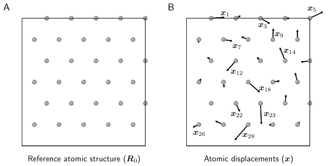
Figure 1: (A) Schematic illustration of the fixed atomic structure $\boldsymbol{R}_{0}$ (grey circles represent atoms) about which displacements $\boldsymbol{x}$ are learned. (B) Displacement vector of atom $i$ is depicted by an arrow labelled $\boldsymbol{x}_{i}$.

We first define the variational free energy associated with an arbitrary probability distribution $q_{\boldsymbol{x}}(\boldsymbol{x})$ of atomic positions $\boldsymbol{x}$ with the potential energy $U(\boldsymbol{x})$ as follows

$$F[q_{\boldsymbol{x}}(\boldsymbol{x})]=\mathbb{E}_{\boldsymbol{x}\sim q_{\boldsymbol{x}}(\boldsymbol{x})}\left[U(\boldsymbol{x})+k_{B}T\ln q_{\boldsymbol{x}}(\boldsymbol{x})\right].$$ (9)

For the case where $q_{\boldsymbol{x}}(\boldsymbol{x})$ is the Boltzmann distribution $\mu_{\boldsymbol{x}}(\boldsymbol{x})$, the variational free energy is the same as the Helmholtz free energy as given by Equation (4). Furthermore, equilibrium statistical mechanical consideration guarantees that the Boltzmann distribution is the unique minimizer of the variational free energy Equation (9). Thus, the variational free energy is an appropriate loss function to optimize the parameters $\Theta$ of the mappings, and thus to make distribution $q_{x}(\boldsymbol{x})$ close to the Boltzmann distribution $\mu_{\boldsymbol{x}}(\boldsymbol{x})$. The variational free energy can also be expressed in terms of the base distribution as

$$F(\Theta) =\mathbb{E}_{\boldsymbol{z}\sim\mu_{\boldsymbol{z}}(\boldsymbol{z})}\left[U\left(\boldsymbol{f}_{zx}(\boldsymbol{z};\Theta)\right)+k_{B}T\ln\mu_{z}\left(\boldsymbol{z}\right)-k_{B}T\ln\gamma_{zx}(\boldsymbol{z};\Theta)\right].$$ (10)

We notice that the second term does not depend on the parameters $\Theta$, and thus can be removed to obtain the following loss function that is used in this work as a metric to optimize the mapping

$$L\left(\Theta\right)=\mathbb{E}_{\boldsymbol{z}\sim\mu_{\boldsymbol{z}}(\boldsymbol{z})}\left[U\left(\boldsymbol{f}_{zx}(\boldsymbol{z};\Theta)\right)-k_{B}T\ln\gamma_{zx}(\boldsymbol{z};\Theta)\right].$$ (11)

The first term in the above loss function tries to reduce the potential energy of and, therefore, narrow the transformed distribution $q_{\boldsymbol{x}}(\boldsymbol{x})$ towards the lower energy atomic configurations; the second term, however, competes with the first term to encourage the spreading of the distribution $q_{\boldsymbol{x}}(\boldsymbol{x})$. The strength of the second term depends on the temperature $T$ and acts as a measure of the entropy of the system. We further note that loss function $L$ differs from the variational free energy of the transformed distribution $q_{\boldsymbol{x}}(\boldsymbol{x})$ only by a constant term which, as evident from Equation (10), is temperature times entropy of the base distribution. As shown by Noé et al [24], the same loss function, Equation (11), can also be obtained by minimizing the Kullback-Leibler divergence between the transformed distribution $q_{\boldsymbol{x}}(\boldsymbol{x})$ and the target Boltzmann distribution $\mu_{\boldsymbol{x}}(\boldsymbol{x})$.

The translation invariance of potential potential energy function $U(x)$ presents a problem regarding the motion of the center of mass of the atoms. Since potential energy remains unchanged for a rigid body motion, the distribution of atomic displacements $\boldsymbol{x}$ optimized using the loss function, Equation (11), could lead to uncontrolled motion of the center of mass and result in higher entropic contribution to the overall free energy. This could further result in weakly diverging learning regime. To avoid these problems, we propose to augment the potential energy function $U(x)$ by adding a harmonic potential energy term for the center of mass motion. Therefore, we optimize the parameters $\Theta$ under the total potential energy function

$$U_{\rm aug}(\boldsymbol{x})=U(\boldsymbol{x})+\frac{1}{2}k_{\rm com}|\boldsymbol{x}_{\rm com}|^{2},$$ (12)

where $k_{\rm com}$ is the stiffness of the harmonic spring attached to the center of mass, and $\boldsymbol{x}_{\rm com}$ is the displacement vector of the center of mass. The additional contribution to the total free energy (including momentum term) arising due to the harmonic motion of the center of mass has the following analytical form

$$F_{\rm com}=-3k_{B}T\ln\left(\frac{k_{B}T}{\hbar}\sqrt{\frac{Nm}{k_{\rm com}}}\right),$$ (13)

which is subtracted from the overall free energy to obtain the final free energy as described in the next section.

4 Learned distribution as a reference state for free energy computation

As discussed in the preceding sections, normalizing flow produces a distribution of atomic configurations $q_{\boldsymbol{x}}(\boldsymbol{x})$ by transforming a simple base probability distribution $\mu_{\boldsymbol{z}}(\boldsymbol{z})$. The variables $\boldsymbol{z}$ and $\boldsymbol{x}$ are understood as denoting the atomic displacements from a fixed atomic structure $\boldsymbol{R}_{0}$ with potential energy $U_{0}$. We can interpret these two distributions as two thermodynamic systems in the canonical ensemble with their respective potential energy functions. We consider that the base probability distribution $\mu_{\boldsymbol{z}}(\boldsymbol{z})$ defines thermodynamic system I (TSI) with associated potential energy function $U^{\rm I}(\boldsymbol{z})$, i.e.

$$\mu_{\boldsymbol{z}}(\boldsymbol{z})=\frac{1}{Z_{\rm I}}\exp\left(-\frac{U^{\rm I}(\boldsymbol{z})}{k_{B}T}\right).$$ (14)

We further assume that due to the simplicity of the base distribution, its partition function $Z_{\rm I}$ is exactly known and, in return, its free energy $F_{\rm I}\equiv-k_{B}T\ln Z_{I}$. For instance, if every $3N$ components of $\boldsymbol{z}$ are normally distributed with zero mean and unit standard deviation, as used in this work, the corresponding potential energy function is $U^{\rm I}(\boldsymbol{z})=\boldsymbol{z}^{2}/2$, and partition function takes the value $Z_{\rm I}=(2\pi k_{B}T)^{3N/2}$.

The transformed distribution obtained from the application of normalizing flow on the base distribution is termed thermodynamic system II (TSII). To obtain the potential energy function of this TSII, we make use of Equations (7) and (14) to write

$$q_{\boldsymbol{x}}(\boldsymbol{x}) =\frac{1}{Z_{I}}\exp\left(-\frac{U^{\rm II}(\boldsymbol{x})}{k_{B}T}\right),$$ (15)

$$\text{where }U^{\rm II}(\boldsymbol{x}) =U^{\rm I}\left(\boldsymbol{f}_{xz}(\boldsymbol{x})\right)-k_{B}T\ln\gamma_{xz}(\boldsymbol{x}).$$

It is clear from the above equation that under the canonical ensemble, the potential energy function of TSII is $U^{\rm II}(\boldsymbol{x})$. Under this potential energy function free energy of TSII is the same as that of TSI, i.e. $F^{\rm II}=F^{\rm I}\equiv-k_{B}T\ln Z_{\rm I}$, which is known by design.

We note that the bijective mapping function $\boldsymbol{f}_{zx}$ is learned such that TSII should approach ever more closely the target Boltzmann distribution $\mu_{\boldsymbol{x}}(\boldsymbol{x})$ with the augmented potential energy function $U_{\rm aug}(\boldsymbol{x})$. This further implies that the potential energy of TSII, $U^{\rm II}(\boldsymbol{x})$, approximates the augmented potential energy function $U_{\rm aug}(\boldsymbol{x})$ except for an additive constant, i.e $U^{\rm II}(\boldsymbol{x})\approx U_{\rm aug}(\boldsymbol{x})+{\rm constant}$. This property is shown in Figure 3, where the learned energy $U^{\rm II}(\boldsymbol{x})$ of the generated configurations obtained from a trained normalizing flow has a strong correlation with the ‘real’ augmented potential energy $U_{\rm aug}(\boldsymbol{x})$.

However, due to limitations in the expressive power of the mapping function (e.g. the limited number of parameters) and computational resources (limiting the training time), the transformed distribution $q_{\boldsymbol{x}}(\boldsymbol{x})$ would not be exactly the same as the target distribution $\mu_{\boldsymbol{x}}(\boldsymbol{x})$, although they should be close. This closeness, nevertheless, is well suited to be exploited in the framework of free energy perturbation methods, as discussed in Section 2, to compute free energy of the system of interest.

Since, as shown in the preceding paragraphs, the potential energy and free energy of TSII are fully accessible, it can be used as a reference system to compute free energy of the target system with the augmented potential energy function $U_{\rm aug}(\boldsymbol{x})$ given by Equation (12). Using Equation (6), configurational free energy of the target system can be determined as

$$F_{\boldsymbol{X},\text{aug}} =-k_{B}T\ln\mathbb{E}_{\boldsymbol{x}\sim q_{\boldsymbol{x}}(\boldsymbol{x})}\left[\exp\left(-\frac{U_{\rm aug}(\boldsymbol{x})-U^{\rm II}(\boldsymbol{x})}{k_{B}T}\right)\right]+F^{\rm II},$$ (16)

$$=-k_{B}T\ln\mathbb{E}_{\boldsymbol{z}\sim\mu_{\boldsymbol{z}}(\boldsymbol{z})}\left[\exp\left(-\frac{U_{\rm aug}\left(\boldsymbol{f}_{zx}(\boldsymbol{z})\right)-U^{\rm I}\left(\boldsymbol{z}\right)-k_{B}T\ln\gamma_{zx}(\boldsymbol{z})}{k_{B}T}\right)\right]-k_{B}T\ln Z_{\rm I},$$

Thus, Equation (16) offers a way to compute the exact unbiased free energy of the system. Estimation of the average required in the first term of Equation (16) over the base distribution can be performed efficiently by generating multiple samples from the distribution $\mu_{\boldsymbol{z}}(\boldsymbol{z})$ in parallel. We further remark that exactly the same Equation (16) can also be obtained through the route of importance sampling which is frequently-used reweighting method in statistics [24].

After determining the configurational part of the free energy from Equation (16), we add the momentum contribution Equation (3) and subtract the center of mass contribution Equation (13) to obtain the final unbiased total free energy

$$F=F_{\boldsymbol{X},\text{aug}}+F_{\boldsymbol{P}}-F_{\rm com}$$ (17)

The workflow of the normalizing flow from base distribution to computing the free energy of the target system is laid out schematically in Figure 2.

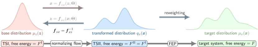
Figure 2: Schematic illustration of various steps involved in free energy the free energy of the system of interest using the normalizing flow. The simple base distribution representing TSI is transformed into a distribution representing TSII. TSII has the same free energy as TSI, and the associated potential energy function of TSII is close to that of the target system. A reweighting procedure based on the free energy perturbation (FEP) method is finally applied to TSII to determine the free energy of the target system.

5 Application to perfect crystal and vacancy formation in diamond-cubic Si

In this section we apply the normalizing flow framework, as presented in the preceding sections, to determine the temperature-dependent free energy associated with the real system of interest. We first compute the Gibbs free energy at zero stress condition, which is equal to the Helmholtz free energy, of perfect diamond-cubic Si crystal.

We then turn our attention to vacancy, a crystalline defect, which is fundamental in controlling materials transport and determining several mechanical properties. Vacancies play a prominent role at high temperatures by diffusing in the material in the field of other crystalline defect such as grain boundaries and dislocations. Thus quantifying the thermodynamic properties of vacancy is necessary to build an understanding of its wide-ranging influence on material properties. We particularly focus on the formation free energy which is an important thermodynamic quantity governing the equilibrium population of vacancy at finite temperatures.

5.1 Computational details

A periodic simulation box is constructed by replicating the diamond-cubic unit cell (each containing 8 atoms with 0 K lattice parameter 5.430 Å) three times in all three directions. The simulation box thus contain 216 atoms. For vacancy study, the vacancy is introduced by removing one atom from the simulation box of perfect crystal and minimize the energy keeping the simulation box dimensions fixed. Interatomic interactions of Si atoms are described by using Stillinger–Weber (SW) potential of which parameters are listed in Ref. [34]. To compute the Gibbs free energy at finite temperatures, we first compute the equilibrium lattice parameters at corresponding temperatures by running isobaric $NPT$ simulations at zero stress conditions and averaging the simulation box sizes. The simulation boxes constructed with these finite temperature lattice parameters are the fixed atomic structures $\boldsymbol{R_{0}}$ used in the normalizing flow framework about which the displacements $\boldsymbol{x}$ are learned. The Helmholtz free energy computed at the fixed volume of zero stress is the same as Gibbs free energy at zero stress.

We now describe the structure and various components involved in RealNVP based normalizing flow used in this work. The base distribution for perfect crystal $\mu_{\boldsymbol{z}}(\boldsymbol{z})$ is a multivariate Gaussian over 648 (3$\times$216) dimensional random vector $\boldsymbol{z}$ with zero mean and identity covariance matrix, i.e. no correlation exists among its components. For vacancy, the base distribution is defined over 645-dimensional (3 $\times$ 215) space. Successive transformations, as described in A, are applied on $\boldsymbol{z}$ sampled from $\mu_{\boldsymbol{z}}(\boldsymbol{z})$ to obtain the displacement vector $\boldsymbol{x}$. To apply the coupling layer of RealNVP, we divide the vector into two halves, each having 324 components. In each coupling layer, scaling function $\boldsymbol{s}(\cdot;\Theta)$ and translation function $\boldsymbol{t}(\cdot;\Theta)$ are two neural networks whose hyperparameters are listed in Table 1. In total we apply ten coupling layers, each with its own separate set of parameters in scaling and translation functions. We finally multiply thus transformed vector with an optimizable scalar parameters to control the initial magnitude of the displacement vectors $\boldsymbol{x}$. This step of scaling is necessary to prevent the unreasonably large displacement that can cause energy to become too high and lead to instability in the optimization process.

Table 1: Hyperparameters of the two neural networks: scaling $\boldsymbol{s}$ and translation $\boldsymbol{t}$.(see A for details) These hyperparameters are the same across 30 Coupling layers used in the mapping function. The optimizable parameters, however, are tuned independently in all the coupling layers during training, i.e. we don’t us parameter sharing among the neural networks.

neural network	$\boldsymbol{s}$()	$\boldsymbol{t}()$
input dimension	324	324
output dimension	324	324
number of hidden layers	3	3
hidden layer dimension	500	500
non linearity	tanh	LeakyReLU

During the training of the normalizing flow, 128 samples from the base distribution $\mu_{\boldsymbol{z}}(\boldsymbol{z})$ are generated to modify parameters based on the gradient of the loss function of Equation (11). The training is performed using ADAM algorithm with multiple learning rates: $10^{-3}$ for the first 4000 steps, $10^{-4}$ for the next 4000 steps and $10^{-5}$ for the last 2000 steps. After training the normalizing flow, the total free energy is determined using Equation (17) where average is calculated using 10000 samples drawn from the base distribution.

The computation of energies of atomic systems are performed by using open source MD code LAMMPS [35]; and the normalizing flow, including neural networks, is constructed and trained using the python library Pytorch [36].

5.2 Results

This section presents the results obtained from the application of the normalizing flow to perfect crystal and vacancy formation in diamond-cubic Si.

5.2.1 Gibbs free energy of perfect diamond-cubic crystal

Figure 3 shows the comparison between the learned potential energy $U^{\rm II}(\boldsymbol{x})$ of TSII, Equation (15), and the augmented potential energy function $U_{\rm aug}(\boldsymbol{x})$, Equation (12), for the atomic configurations $\boldsymbol{x}$ generated from the normalizing flow trained at 2000 K. The plot of the joint distribution shows a strong correlation between the two energy functions. Thus the normalizing flow is able to learn a thermodynamic system TSII with the potential energy function $U^{\rm II}(\boldsymbol{x})$ close to the augmented potential energy function $U_{\rm aug}(\boldsymbol{x})$.

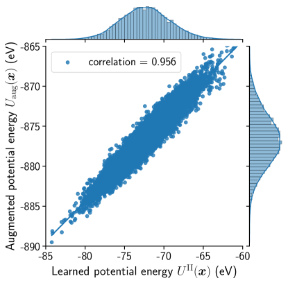
Figure 3: Joint distribution of the augmented potential energy function $U_{\rm aug}(\boldsymbol{x})$ and the learned potential energy $U^{\rm II}(\boldsymbol{x})$ of TSII. The atomic configurations $\boldsymbol{x}$ are generated from the normalizing flow trained at 2000 K. The potential energy $U^{\rm II}(\boldsymbol{x})$ of of TS II has strong correlation with the augmented potential energy $U_{\rm aug}(\boldsymbol{x})$ that includes energy from the SW potential and energy due to harmonic center of mass potential.

We now present the Gibbs free energy of Si computed from normalizing flow framework, and compare with the values computed from the adiabatic switching method following Ref. [37]. The Gibbs free energy at a particular temperature is equal to Helmholtz free energy determined using the equilibrium lattice constant at the corresponding temperature. Total Free energy is given in Equation (3), in which the configurational free energy contribution is evaluated using Equation (16).

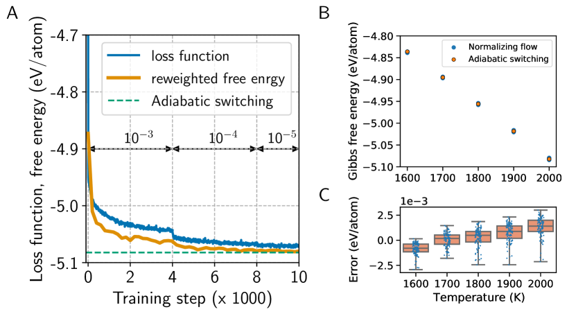
Figure 4: (A) Variation in loss function, including momentum contribution and entropy of base distribution, with training steps at 2000 K temperature is plotted with blue line. Multiple learning rates($10^{-3},10^{-4}$ and $10^{-5}$) used during different stages of training are shown. Change in the Gibbs free energy, obtained by the perturbation procedure, with training steps is also plotted with orange color. The free energy calculations using the importance sampling reweighting are performed after every 200 training steps. The green dashed horizontal line shows the free energy obtained from the adiabatic switching method. (B) Blue circles show a scatter plot of 100 difference calculations of the Gibbs free energy per atom using the normalizing flow framework as a function of temperature. The Gibbs free energy values as computed from the adiabatic switching method are shown with orange circles for comparison. (C) Plot of the distribution of the difference between normalizing flow and adiabatic switching values for 100 different values obtained fom the normalizing flow.

Figure 4(A) presents the variation in the loss function as a function of training steps. It is clear that the loss function decreases during the training. At each training step, 128 independent random samples are generated to compute the correction in parameters according to the gradient signal obtained from the loss function. Thus, the whole learning framework is that of unsupervised learning, and requires no prior data set. We also show in Figure 4 (A) the variation in the total free energy, computed using Equation (16) as training proceeds. This free energy is computed after every 200 steps by averaging over 1000 samples generated from the normalizing flow. The free energy converges near the value obtained from the adiabatic switching method. The free energy values are presented in Table 2 for both normalizing flow and adiabatic switching methods.

Figure 4(B) shows the total Gibbs free energy, including momentum contribution as depicted in Equation (3), of a perfect diamond cubic Si crystal at temperatures ranging from 1600 to 2000 K. Since we are using finite number of samples (10000), the free energy computed from Equation (17) is itself stochastic. Therefore, we compute the free energy for 100 different sets of 10000 random samples generated from the trained normalizing flow. We also show the Gibbs free energy of the same system by using the adiabatic switching method [37]. Since the scatter in the normalizing values is too small (of the order of $10^{-3}$ eV/atom) to be visible at the scale of the figure, we show the distribution of the difference between 100 normalizing flow values and adiabatic switching value in Figure 4(C). The result from adiabatic switching is just from one switching simulation (for $10^{6}$ MD steps) and we didn’t attempt to quantify its error. However, both results show good agreement with each other establishing that normalizing flow can be employed to determine free energies accurately and efficiently.

Table 2: Gibbs free energy per atom (eV/atom) as a function of temperature of perfect diamnond-cubic Si crystal as computed from the normalizing flow and the adiabatic switching methods. We list only the average values of the free energies obtained from both methods.

Temperature (K)	1600	1700	1800	1900	2000
Normalizing flow	-4.8369	-4.8951	-4.9556	-5.0175	-5.0809
Adiabatic switching	-4.8360	-4.8951	-4.9559	-5.0183	-5.0822

We now compare the computational costs of the two free energy methods as measured in both wall-clock time and number of potential function evaluations. The training of the normalizing flow takes around 6.5 hours while computing the free energy using Equation (17) (reweighting is performed with 10000 samples) using the trained normalizing flow takes around 2 minutes. On the other hand, the adiabatic switching method takes around 45 minutes to perform one pair of forward and backward switching between harmonic and real crystals. Thus, despite a little longer training process, the normalizing can be more efficient in collecting a large statistics from the trained normalizing flow. We, however, want to emphasize that we did not invest much effort in optimizing the training process and shortening the training time. Furthermore, one million evaluations of potential energy and atomic forces were performed during the normalizing flow training step; and one adiabatic switching trajectory also involves one million molecular dynamics step. The fact that we need a smaller number of samples (10000 in this work) to compute reweighted free energy using the trained normalizing flow as opposed to the one million MD steps of the adiabatic switching further emphasizes the efficiency of the normalizing flow framework.

5.2.2 Formation free energy of monovacancy

To compute the formation free energy of monovacancy at finite temperatures, we train two normalizing flows: one for the perfect crystal with and another for the crystal containing a vacancy. After training the two normalizing flows, the free energies of the two systems are computed using Equation (17). The formation free energy of monovacancy $F_{\rm f}^{\rm vac}$ is then computed as

$$F_{\rm f}^{\rm vac}=F^{\rm vac}-\frac{N-1}{N}F^{\rm per},$$ (18)

where $F^{\rm vac}$ is the free energy of the crystal containing a vacancy, $F^{\rm per}$ is the free energy of the perfect crystal, and $N$ is the number of atoms in the prefect crystal ($N=216$ in this work).

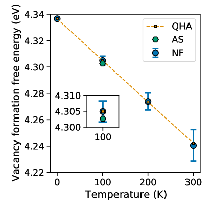
Figure 5: Temperature dependent formation free energy of monovacancy in diamond cubic Si crystal at zero stress condition. Free energies are computed from three independent methods: quasi harmonic approximation (QHA), adiabatic switching (AS) (at $100$ K only), and normalizing flow (NF). The error-bar for the normalizing flow calculations show the standard deviation for 100 different reweighting calculations, each involving 10000 samples. The inset shows the zoomed-in plot of different values of the vacancy formation free energy at 100 K as obtained from the three different methods.

Figure 5 shows the formation free energy of monovacancy at temperatures ranging from 0 to 300 K in diamond-cubic Si as determined from three independent methods: normalizing flow (NF), quasi harmonic approximation (QHA) [38, 39], and adiabatic switching method. The reasons for focusing onto the relatively lower temperatures are two-fold. First is to avoid the complication arising from the vacancy diffusion [40, 41]. Indeed, we found that at temperatuers above $100$ K, the vacancy jumps during the adiabatic switching simulation, producing very large error bars for the free-energy estimate. This makes our current implementation of the adiabatic switching not applicable to vacancy formation free energy calculation above $100$ K. Second, the quasi harmonic approximation becomes reasonably accurate at lower temperatures and thus provides a good reference value for the comparison.

Table 3: Variation of the formation free energy (eV) of monovacancy in diamnond-cubic Si crystal at zero stress condition with temperature as determioned from the normalizing flow and the quasi harmonic approximation methods. The adiabatic switching method is able to provide the vacancy formation free energy only at 100 K temprature due to the observation of the vacancy diffusion at higher temperatures. The value at 0 K is obtained by minimizing the potential energy. The values shown in the table correspond to the average free energy of monovacancy formation determined from the three methods.

Temperature (K)	0	100	200	300
Normalizing flow	4.3366	4.3049	4.2738	4.2405
Quasi harmonic approximation	4.3366	4.3049	4.2735	4.2422
Adiabatic switching	4.3366	4.3026	-	-

From Figure 5, it is manifest that the three methods employed to compute the free energy agree reasonably well establishing the capacity of the normalizing flow to be used in computing the temperature dependent free energy of crystalline defects. From the slope of the vacancy formation energy as a function of temperature, we obtain the formation entropy of the vacancy as 3.72 $k_{B}$. The formation free energies of monovacancy at temratures ranging from 0 to 300 K are listed in Table 3.

6 Conclusion and discussion

In this work, we demonstrated that normalizing flow based framework can be employed to compute reasonably accurate free energy for a solid. Specifically, we computed the zero stress Gibbs free energy of diamond cubic Si at temperatures from 1600 to 2000 K, and showed that there is a good agreement with the available literature values.

We further show that the normalizing flow can be used to determine the formation free energy of monovacancy defect in diamond-cubic crystal at temperatures ranging from 0 to 300 K. This is particularly encouraging due to the fact that material properties emerges from the finite-temperature behavior of various crystalline defects and their mutual interactions, i.e. vacancies, interstitials, solutes, dislocations, stacking fault etc. The challenges involved with computing the free energy associated with defects often leads to resorting to the approximation of the defect free energy by potential energy or tractable local harmonic approximation [42, 43, 44, 45, 46, 47]. The accuracy of such approximation becomes questionable at high temperatures where the anharmonic nature of underlying potential energy function begins to show appreciable effect [41]. Thus the normalizing flow framework is promising in efficient quantification of the finite-temperature mechanisms associated with various crystalline defects, and, in turn, aiding in understanding, controlling and engineering technologically important materials.

Computing the vacancy formation energy at high temperatures is challenging due to issues arising from the diffusion process [41]. As an example in case, we observe the diffusion of vacancy during the adiabatic switching process even at temperatures as low as 200 K. We do not encounter the vacancy diffusion in the normalizing flow framework till 300 K temperature. This is presumably caused by the setup of the problem in which we learn distribution of atomic displacements about a fixed metastable reference state instead of evolving the whole system iteratively as done in MD and MC simulations. Furthermore, the additional constraining of the center of mass by introducing a harmonic potential may also penalize any atom undergoing a systematic large displacement over and above the random thermal fluctuations. However, the framework as presented in this work does not guarantee to prevent the vacancy diffusion entirely at arbitrarily temperatures, and we, therefore, must practice care while investigating defect having multiple metastable states separated by relatively low energy barrier.

A comparison of the time taken by the normalizing flow and the adiabatic switching shows that while the training of the normalizing flow takes a relatively long time, the normalizing can still be much more efficient in collecting a large statistics to obtain reliable results. We, further note that the training time of the normalizing flow can further be improved by optimizing the various steps involved in the training. For example, we use the CPU serial version of LAMMPS in this work to compute energy and forces of the generated atomic configurations. This entails the transfer of data between GPU and CPU during each energy and force computation step. The GPU version of LAMMPS could be leveraged to accelerate the training process. Moreover, various hyperparameters involved in the normalizing flow architecture - learning rate, number of coupling layers, number of hidden dimensions and layers - can be optimized to speed up the training and inference step enhancing the efficiency of the normalizing flow even further.

The normalizing flow has been shown to transform a simple base distribution into a distribution close to the target Boltzmann distribution. We show that the normalizing flow produces a thermodynamic system with known free energy and its associated potential energy function is close to the thermodynamic system under investigation. This enables the use of the learned thermodynamic system as a reference state to determine the free energy of the system of interest.

The reweighting procedure, necessitated by the difference between the transformed (reference) and the target distribution, was performed using the importance sampling or the free energy perturbation method. This is the simplest possible reweighting which still provides accurate results. Since we have access to the normalized probability density of the transformed distribution, more elaborate procedures could be used for the reweighting, for example adiabatic switching [11] and annealed importance sampling [48].

The normalizing flow along with reweighting by importance sampling can also be understood as the targeted free energy perturbation method as described in Ref. [49]. Basically, the transformed distribution is a learned reference system rather than designed a priori. This obviates the work involved in computing various properties to be included in the reference system. For instance we would need to have access to the normal mode frequencies of the target system to setup a harmonic approximation-crystal as the reference system. Thus normalizing flow provides a workflow to obtain an optimized reference system in a principled manner for use in the subsequent free energy perturbation methods.

Training of the normalizing flow proceeds in a unsupervised manner. Data to train the network are generated from the base distribution, and thus are unlimited. Each training step encounters new set of randomly sampled data. All these features reduces the possibility of overfitting of the neural networks.

Furthermore, normalizing flows provide a way to efficiently generate equilibrium samples from the Boltzmann distribution using the Metropolis-Hastings algorithm [26]. In this scheme, transformed distribution can be used to generate proposals at each step. As the transformed distribution is close to the target, the acceptance probability of the proposed configurations would be much higher, and the generated samples will have small correlation with good mixing. Moreover, the proposal can be generated in parallel accelerating the process significantly.

In this work, we used RealNVP as the invertible mapping function. RealNVP has advantage in that its operations are quite simple which leads to efficient learning regime. However, RealNVP has some restriction in its expressivity, necessitating composition of several function units, resulting in a large number of parameters. Other more complex and universal mapping functions have been proposed in the literature. However, a systematic study into their memory footprints versus ease of training still needs to be undertaken in the context of free energy computation of atomic systems.

Modeling of extended crystalline defects, such as dislocation, grain boundaries, and their interactions can require thousands to millions of atoms [50, 51]. Thus, application of normalizing flow based algorithms to the extended crystalline solid system with defect may suffer from the scalability of the existing normalizing flow algorithms: the number of parameters in the deep neural network to be learned scales with square of the number of atoms. Thus, atomic modeling of the crystalline solids through the normalizing flow algorithms requires further modifications and will be addressed in future work.

This work has established that normalizing flow provides an efficient way to determine accurate free energy of solid systems. We believe that this normalizing flow framework would help in gaining a deeper understanding of various finite temperature mechanisms underlying wide range of crucial behavior of crystalline solids, and in turn facilitate the design of new class of technologically important materials.

Appendix A Form of the mapping function: real valued non volume preserving (RealNVP) mapping

Here, we describe the form of the mapping function $\boldsymbol{f}_{zx}(\boldsymbol{z})$ itself which is the critical component of normalizing flow. The form of the mapping function should be: invertible, which is intrinsic to the basic working of normalizing flow; expressive, i.e. ability to approximate arbitrarily complex probability distribution function; efficient in computing the Jacobian determinant, i.e. determining the determinant of the jacobian of the mapping function should not entail heavy computational resources and time which is essential for tractable and feasible learning/optimization regime of parameters $\Theta$.

Several mapping functions have been proposed in the literature satisfying the above three properties in varying degrees [22, 23]. In this work we use the so-called real valued non volume-preserving (RealNVP) mapping, proposed by Dinh et al [52] to transform the base Gaussian distribution. which is also used in Ref. [24] The transform of $\boldsymbol{z}$ variable in RealNVP takes place as follows

$$\boldsymbol{x}_{1:3n} =\boldsymbol{z}_{1:3n},$$ (A.19)

$$\boldsymbol{x}_{3n+1:3N} =\boldsymbol{z}_{3n+1:3N}\odot\exp\left(\boldsymbol{s}\left(\boldsymbol{z}_{1:3n};\Theta\right)\right)+\boldsymbol{t}\left(\boldsymbol{z}_{1:3n};\Theta\right),$$

where $\odot$ is notation for Hadamard or element-wise product; $\boldsymbol{s}:\mathbb{R}^{3n}\rightarrow\mathbb{R}^{3N-3n}$ and $\boldsymbol{t}:\mathbb{R}^{3n}\rightarrow\mathbb{R}^{3N-3n}$ are, respectively, scaling and translation functions that contain all the parameters of the mapping function. There is no restriction on these two functions and can possess any level of complexity. In this work these rwo functions are modeled as two deep neural networks. The operation of Equation (A.19) is schematically depicted in Figure 1(A). It can be readily checked that this mapping is invertible and inverse can be computed quite easily. The Jacobian matrix of the transformation is given by

$$\frac{\partial\boldsymbol{x}}{\partial\boldsymbol{z}}=\begin{bmatrix}\begin{array}[]{c|c}\mathbb{I}_{3n\times 3n}&\mathbb{O}_{3n\times 3N-3n}\\[10.00002pt] \hline\cr\\ \frac{\partial\boldsymbol{x}_{3n+1:3N}}{\partial\boldsymbol{z}_{1:3n}}&\text{diag}\left(\exp\left(\boldsymbol{s}(\boldsymbol{z}_{1:3n})\right)\right)\end{array}\end{bmatrix},$$ (A.20)

where $\mathbb{I}_{3N\times 3N}$ is an identity matrix, and $\mathbb{O}_{3n\times 3N-3n}$ is a zero matrix. Since the Jacobian matrix is a triangular matrix, its determinant is simply the product of the diagonal terms, which is

$$\gamma_{zx}(\boldsymbol{z}) =\left|\det\left(\frac{\partial\boldsymbol{x}}{\partial\boldsymbol{z}}\right)\right|=\prod_{i=1}^{3N-3n}\exp\left(s_{i}(\boldsymbol{z}_{1:3n})\right),$$ (A.21)

$$\ln\gamma_{zx}(\boldsymbol{z}) =\sum_{i=i}^{3N-3n}s_{i}\left(\boldsymbol{z}_{1:3n}\right).$$

Therefore, the Jacobian determinant of the mapping can be efficiently determined without any additional expensive computation.

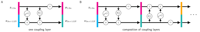
Figure 1: (A) A schematic depiction of the operation of single coupling layer that transform $\boldsymbol{z}$ into $\boldsymbol{x}$. Note that one half (magenta colored) of the $\boldsymbol{z}$ vector is kept unchanged, and only the other half (cyan colored) is transformed. (B) To increase the expressivity of RealNVP, multiple coupling layers are composed in sequence. Note that the unchanged half is alternated to transform the whole vector after two operations of coupling layer. $\boldsymbol{s}()$ and $\boldsymbol{t}$() functions appearing in coupling layers are modeled by two neural networks, and each coupling layer can have its own independent parameters.

One limitation of the mapping function presented in Equation (A.19) is that one part of the vector $\boldsymbol{z}$ is untransformed which clearly imposes severe restriction on the class of distribution function that can be obtained from this mapping. To resolve this expressivity issue to some extent, we can compose many such functions in sequence. One function unit being composed is called coupling layer in the normalizing flow literature. The part of the vector that is kept unchanged is alternated between subsequent coupling layers as shown in Figure 1(B). Expressivity of the overall mapping can be increased by applying many coupling layers. Furthermore, parameters of all the coupling layers need not be different and can be shared among compatible layers.

The invertibility of the overall mapping is ensured by the fact that all the coupling layers being composed are invertible. Computing inverse itself is easy because inverse of a composition of function is composition of inverse of the functions in reverse order. The Jacobian determinant of the overall mapping is computed by using the fact that determinant of the Jacobian of composition of functions is the product of the Jacobian of the constituent functions involved in the composition. To write these facts in mathematical form, suppose $\boldsymbol{x}$ is obtained by applying $p$ number of functions $f_{1},f_{2},f_{3},\dots,f_{p}$ is in sequence, i.e. $\boldsymbol{x}=f_{p}\circ f_{p-1}\circ\dots\circ f_{1}(\boldsymbol{z})$. The inverse and the Jacobian determinant of the mapping is expressed as

$$\boldsymbol{z} =f^{-1}_{1}\circ f^{-1}_{2}\circ\dots\circ f^{-1}_{p}(\boldsymbol{x}),$$ (A.22)

$$\gamma_{zx} =\prod_{i=1}^{p}\gamma_{i},$$

where $\gamma_{i}$ is the Jacobian determinant of the function $f_{i}$ evaluated at its input.

RealNVP is quite efficient in performing computations as it involves only a few simple mathematical operations. However this efficiency comes at the cost of reduced expressivity. To approximate a complex probability distribution functions, a large number of coupling layers may be required. For a detailed analysis of the expressivity of RealNVP and other mapping commonly used in normalizing flow, the readers are encouraged to consult Refs. [22, 23].

References

- [1] M. J. Gillan, D. Alfè, J. Brodholt, L. Vočadlo, and G. D. Price. First-principles modelling of Earth and planetary materials at high pressures and temperatures. Reports Prog. Phys., 69(8):2365–2441, 2006.
- [2] J. Q. Broughton and X.P. Li. Phase diagram of silicon by molecular dynamics. Phys. Rev. B, 35(17):9120–9127, 1987.
- [3] Wei Cai and William D Nix. Imperfections in Crystalline Solids. MRS-Cambridge Materials Fundamentals. Cambridge University Press, 2016.
- [4] George H. Vineyard. Frequency factors and isotope effects in solid state rate processes. J. Phys. Chem. Solids, 3(1-2):121–127, 1957.
- [5] D. Caillard and J. L. Martin. Thermally Activated Mechanisms in Crystal Plasticity, volume 8 of Pergamon Materials Series. Pergamon, 2003.
- [6] Vasily Bulatov and Wei Cai. Computer Simulations of Dislocations (Oxford Series on Materials Modelling). Osmm Series. Oxford University Press, Inc., USA, 2006.
- [7] D Frenkel and B Smit. Understanding Molecular Simulation: From Algorithms to Applications. Computational science. Elsevier Science, 2001.
- [8] M E Tuckerman. Statistical Mechanics: Theory and Molecular Simulation. Oxford graduate texts. Oxford University Press, 2011.
- [9] Christophe Chipot and Andrew Pohorille, editors. Free Energy Calculations, volume 86 of Springer Series in Chemical Physics. Springer-Verlag Berlin Heidelberg, 2007.
- [10] John G. Kirkwood. Statistical mechanics of fluid mixtures. J. Chem. Phys., 3(5):300–313, 1935.
- [11] Masakatsu Watanabe and William P. Reinhardt. Direct dynamical calculation of entropy and free energy by adiabatic switching. Phys. Rev. Lett., 65(26):3301–3304, 1990.
- [12] M. de Koning and A. Antonelli. Adiabatic switching applied to realistic crystalline solids: Vacancy-formation free energy in copper. Phys. Rev. B - Condens. Matter Mater. Phys., 55(2):735–744, 1997.
- [13] Rodrigo Freitas, Mark Asta, and Maurice de Koning. Nonequilibrium free-energy calculations of solids using LAMMPS. Comput. Mater. Sci., 112:333–341, 2016.
- [14] C. Jarzynski. Nonequilibrium Equality for Free Energy Differences. Phys. Rev. Lett., 78(14):2690–2693, 1997.
- [15] Li Wen Tsao, Sheh Yi Sheu, and Chung Yuan Mou. Absolute entropy of simple point charge model water by adiabatic switching processes. J. Chem. Phys., 101(3):2302–2308, 1994.
- [16] M. de Koning and A. Antonelli. Einstein crystal as a reference system in free energy estimation using adiabatic switching. Phys. Rev. E - Stat. Physics, Plasmas, Fluids, Relat. Interdiscip. Top., 53(1):465–474, 1996.
- [17] Albert P. Bartók, Sandip De, Carl Poelking, Noam Bernstein, James R. Kermode, Gábor Csányi, and Michele Ceriotti. Machine learning unifies the modeling of materials and molecules. Sci. Adv., 3(12):1–9, 2017.
- [18] Frank Noé, Alexandre Tkatchenko, Klaus Robert Müller, and Cecilia Clementi. Machine learning for molecular simulation. Annu. Rev. Phys. Chem., 71:361–390, 2020.
- [19] Michele Ceriotti, Cecilia Clementi, and O. Anatole Von Lilienfeld. Introduction: Machine Learning at the Atomic Scale. Chem. Rev., 121(16):9719–9721, 2021.
- [20] Ian J Goodfellow, Jean Pouget-Abadie, Mehdi Mirza, Bing Xu, David Warde-Farley, Sherjil Ozair, Aaron Courville, and Yoshua Bengio. Sparse generative adversarial network. Proc. Int. Conf. Neural Inf. Process. Syst. (NIPS 2014)., pages 2672–2680, 2014.
- [21] Danilo Jimenez Rezende and Shakir Mohamed. Variational inference with normalizing flows. 32nd Int. Conf. Mach. Learn. ICML 2015, 2:1530–1538, 2015.
- [22] Ivan Kobyzev, Simon Prince, and Marcus Brubaker. Normalizing Flows: An Introduction and Review of Current Methods. IEEE Trans. Pattern Anal. Mach. Intell., pages 1–1, 2020.
- [23] George Papamakarios, Eric Nalisnick, Danilo Jimenez Rezende, Shakir Mohamed, and Balaji Lakshminarayanan. Normalizing Flows for Probabilistic Modeling and Inference. arXiv, pages 1–60, 2019.
- [24] Frank Noé, Simon Olsson, Jonas Köhler, and Hao Wu. Boltzmann generators: Sampling equilibrium states of many-body systems with deep learning. Science., 365(6457):eaaw1147, 2019.
- [25] M. S. Albergo, G. Kanwar, and P. E. Shanahan. Flow-based generative models for Markov chain Monte Carlo in lattice field theory. Phys. Rev. D, 100(3):34515, 2019.
- [26] Kim A. Nicoli, Shinichi Nakajima, Nils Strodthoff, Wojciech Samek, Klaus Robert Müller, and Pan Kessel. Asymptotically unbiased estimation of physical observables with neural samplers. Phys. Rev. E, 101(2):1–10, 2020.
- [27] Thomas Müller, Brian McWilliams, Fabrice Rousselle, Markus Gross, and Jan Novák. Neural importance sampling. ACM Trans. Graph., 38(5), 2019.
- [28] Hao Xie, Linfeng Zhang, and Lei Wang. Ab-initio study of interacting fermions at finite temperature with neural canonical transformation. arXiv, pages 1–11, 2021.
- [29] Shuo Hui Li and Lei Wang. Neural Network Renormalization Group. Phys. Rev. Lett., 121(26):260601, 2018.
- [30] Robert W Zwanzig. High-Temperature Equation of State by a Perturbation Method. I. Nonpolar Gases. J. Chem. Phys., 22:1420, 1954.
- [31] Tony Lelièvre, Mathias Rousset, and Gabriel Stoltz. Free Energy Computations. IMPERIAL COLLEGE PRESS, 2010.
- [32] Niels Hansen and Wilfred F. Van Gunsteren. Practical aspects of free-energy calculations: A review. J. Chem. Theory Comput., 10(7):2632–2647, 2014.
- [33] Maurice De Koning. Optimizing the driving function for nonequilibrium free-energy calculations in the linear regime: A variational approach. J. Chem. Phys., 122(10), 2005.
- [34] Frank H. Stillinger and Thomas A. Weber. Computer simulation of local order in condensed phases of silicon. Phys. Rev. B, 31(8):5262–5271, 1985.
- [35] S Plimpton. Fast Parallel Algorithms for Short-Range Molecular Dynamics. J. Comput. Phys., 117(1):1–19, 1995.
- [36] Adam Paszke, Sam Gross, Francisco Massa, Adam Lerer, James Bradbury, Gregory Chanan, Trevor Killeen, Zeming Lin, Natalia Gimelshein, Luca Antiga, Alban Desmaison, Andreas Kopf, Edward Yang, Zachary DeVito, Martin Raison, Alykhan Tejani, Sasank Chilamkurthy, Benoit Steiner, Lu Fang, Junjie Bai, and Soumith Chintala. PyTorch: An Imperative Style, High-Performance Deep Learning Library. In H Wallach, H Larochelle, A Beygelzimer, F D’Alché-Buc, E Fox, and R Garnett, editors, Adv. Neural Inf. Process. Syst. 32, pages 8024–8035. Curran Associates, Inc., 2019.
- [37] Seunghwa Ryu and Wei Cai. Comparison of thermal properties predicted by interatomic potential models. Model. Simul. Mater. Sci. Eng., 16(8), 2008.
- [38] R. Ramírez, N. Neuerburg, M. V. Fernández-Serra, and C. P. Herrero. Quasi-harmonic approximation of thermodynamic properties of ice Ih, II, and III. J. Chem. Phys., 137(4):144, 2012.
- [39] Jianjun Xie, Stefano de Gironcoli, Stefano Baroni, and Matthias Scheffler. First-principles calculation of the thermal properties of silver. Phys. Rev. B - Condens. Matter Mater. Phys., 59(2):965–969, 1999.
- [40] Stephen M. Foiles. Evaluation of harmonic methods for calculating the free energy of defects in solids. Phys. Rev. B, 49(21):14930–14938, 1994.
- [41] Bingqing Cheng and Michele Ceriotti. Computing the absolute Gibbs free energy in atomistic simulations: Applications to defects in solids. Phys. Rev. B, 97(5):1–10, 2018.
- [42] Rasool Ahmad, Zhaoxuan Wu, Sébastien Groh, and W. A. Curtin. Pyramidal II to basal transformation of <c + a> edge dislocations in Mg-Y alloys. Scr. Mater., 155:114–118, 2018.
- [43] Rasool Ahmad, Binglun Yin, Zhaoxuan Wu, and W.A. Curtin. Designing high ductility in magnesium alloys. Acta Mater., 172:161–184, jun 2019.
- [44] Rasool Ahmad, Zhaoxuan Wu, and W.A. A Curtin. Analysis of double cross-slip of pyramidal I <c + a> screw dislocations and implications for ductility in Mg alloys. Acta Mater., 183:228–241, 2020.
- [45] Zhaoxuan Wu, Rasool Ahmad, Binglun Yin, Stefanie Sandlöbes, and W. A. Curtin. Mechanistic origin and prediction of enhanced ductility in magnesium alloys. Science., 359(6374):447–452, 2018.
- [46] LeSar R, Najafabadi R, and Srlovitz D J. Finite-Temperature Defect Properties from Free-Energy Minimization. Phys. Rev. Lett., 63(6):624–627, 1989.
- [47] Seunghwa Ryu, Keonwook Kang, and Wei Cai. Predicting the dislocation nucleation rate as a function of temperature and stress. J. Mater. Res., 26(18):2335–2354, 2011.
- [48] Radford M. Neal. Annealed importance sampling. Stat. Comput., 11(2):125–139, 2001.
- [49] C. Jarzynski. Targeted free energy perturbation. Phys. Rev. E - Stat. Physics, Plasmas, Fluids, Relat. Interdiscip. Top., 65(4):5, 2002.
- [50] Luis A. Zepeda-Ruiz, Alexander Stukowski, Tomas Oppelstrup, and Vasily V. Bulatov. Probing the limits of metal plasticity with molecular dynamics simulations. Nature, 550(7677):492–495, 2017.
- [51] Nicolas Bertin, Ryan B. Sills, and Wei Cai. Frontiers in the Simulation of Dislocations. Annu. Rev. Mater. Res., 50:437–464, 2020.
- [52] Laurent Dinh, Jascha Sohl-Dickstein, and Samy Bengio. Density estimation using real NVP. 5th Int. Conf. Learn. Represent. ICLR 2017 - Conf. Track Proc., 2019.