The Warm Neptune GJ 3470b has a Polar Orbit

Abstract

The warm Neptune GJ 3470b transits a nearby ($d=29\,\mathrm{pc}$) bright slowly rotating M1.5-dwarf star. Using spectroscopic observations during two transits with the newly commissioned NEID spectrometer on the WIYN 3.5m Telescope at Kitt Peak Observatory, we model the classical Rossiter-Mclaughlin effect yielding a sky-projected obliquity of $\lambda=98_{-12}^{+15\>\circ}$ and a $v\sin i=0.85_{-0.33}^{+0.27}\,\mathrm{km/s}$. Leveraging information about the rotation period and size of the host star, our analysis yields a true obliquity of $\psi=95_{-8}^{+9\>\circ}$, revealing that GJ 3470b is on a polar orbit. Using radial velocities from HIRES, HARPS and the Habitable-zone Planet Finder, we show that the data are compatible with a long-term RV slope of $\dot{\gamma}=-0.0022\pm 0.0011\,\mathrm{m/s/day}$ over a baseline of 12.9 years. If the RV slope is due to acceleration from another companion in the system, we show that such a companion is capable of explaining the polar and mildly eccentric orbit of GJ 3470b using two different secular excitation models. The existence of an outer companion can be further constrained with additional RV observations, Gaia astrometry, and future high-contrast imaging observations. Lastly, we show that tidal heating from GJ 3470b’s mild eccentricity has most likely inflated the radius of GJ 3470b by a factor of $\sim$1.5-1.7, which could help account for its evaporating atmosphere.

1 Introduction

The stellar obliquity ($\psi$), the angle between the stellar spin axis and a planet’s orbital axis, is an important parameter of an exoplanet system. Although the planets in the solar system are observed to be well-aligned to the spin axis of the Sun (within $7^{\circ}$), exoplanetary systems show a broad range of obliquities, ranging from well-aligned to severely misaligned. These results have been interpreted as clues to their formation (Albrecht et al., 2012). Different mechanisms have been proposed to explain the tilting of planetary orbits, including primordial misalignment between the star and the protoplanetary disk (Lai et al., 2011; Batygin, 2012), nodal precession induced by an inclined companion (Yee et al., 2018), the Von Zeipel-Lidov-Kozai meachanism (Fabrycky & Tremaine, 2007; Naoz, 2016; Ito & Ohtsuka, 2019), planet-planet scattering (Rasio & Ford, 1996; Chatterjee et al., 2008), and secular resonance crossings due to a disappearing disk and a massive outer planetary companion (Petrovich et al., 2020).

Stellar obliquities can be constrained by exploiting the Rossiter-McLaughlin (RM) effect, the alteration of the rotational broadening kernel of the star’s absorption line profiles that occurs during a planetary transit. The RM effect is often observed as a radial velocity anomaly (Triaud, 2018), and has been observed for hundreds of planetary systems. However, the RM effect is primarily sensitive to the sky-projected obliquity ($\lambda$), the angle between the sky projections of the stellar rotation axis and the planet orbital axis. To obtain the three-dimensional obliquity $\psi$, observations of the RM effect generally need to be supplemented with a constraint on the inclination $i_{\star}$ of the stellar rotation axis with respect to the line of sight.

Using a sample of true obliquities $\psi$, Albrecht et al. (2021) found evidence that misaligned systems show a preference for nearly polar orbits ($\psi=80-125^{\circ}$) rather than spanning the full range of possible obliquities. Most of the available sample consists of hot Jupiters because they allow for the most straightforward measurements. However, hot Jupiters are intrinsically rare (Dawson & Johnson, 2018), and it is unclear if planetary systems hosting smaller planets show the same orbital architectures as hot Jupiters. Among the systems studied by Albrecht et al. (2021), a few warm Neptunes ($a/R_{\star}\gtrsim 8$) orbiting cool stars ($T_{\mathrm{eff}}<6100\,\mathrm{K}$) have been observed to have polar orbits, including HAT-P-11b (Sanchis-Ojeda & Winn, 2011), GJ 436b (Bourrier et al., 2018a, 2022), HD 3167c (Dalal et al., 2019; Bourrier et al., 2021), and WASP-107b (Dai & Winn, 2017; Rubenzahl et al., 2021). For three of these planets—HAT-P-11b (Allart et al., 2018), GJ 436b (Kulow et al., 2014; Ehrenreich et al., 2015), and WASP-107b (Allart et al., 2019)—there is evidence for ongoing atmospheric mass loss. Furthermore, two of the planets are known to have outer planetary companions (HAT-P-11b, Yee et al. 2018; and WASP-107b, Piaulet et al. 2021) suggesting that they arrived at their current polar orbits through dynamical interactions.

Here we present observations of the RM effect of the low-density warm Neptune GJ 3470b, which orbits a bright ($V=12.3$, $J=8.8$) M1.5 dwarf star located 29 parsecs away (Bonfils et al., 2012). GJ 3470b is known to be undergoing substantial mass loss (e.g., Bourrier et al., 2018b; Ninan et al., 2020). We performed the precise radial velocity (RV) observations with the recently commissioned NEID spectrograph (Schwab et al., 2016) on the WIYN 3.5m Telescope at Kitt Peak Observatory. Two transits with NEID reveal that GJ 3470b has an RM signal consistent with a polar orbit. Additionally, we detect evidence for a long-term acceleration based on RVs reported in the literature and newly obtained with the Habitable-zone Planet Finder, suggesting the existence of an outer companion in the system. With these measurements, GJ 3470b joins a growing sample of warm Neptunes on polar orbits that are observed to have evaporating atmospheres, suggesting that such systems might share a common formation history involving dynamical interactions with an outer companions in the system (e.g., Bourrier et al., 2018a; Owen & Lai, 2018; Correia et al., 2020; Attia et al., 2021).

2 Stellar Parameters

Table 1 lists the stellar parameters used in this work. To obtain precise estimates of the stellar mass and radius, we performed an SED fit of available literature magnitudes of the star using EXOFASTv2 (Eastman et al., 2019), along with a precise parallax estimate from Gaia. The resulting values agree with the values of the stellar radius ($R=0.48\pm 0.04\,R_{\odot}$) and mass ($M=0.51\pm 0.06\,R_{\odot}$) reported by Biddle et al. (2014).

The stellar rotation period is particularly important for this RM analysis given the low $v\sin i$ we measure of $v\sin i=0.85_{-0.33}^{+0.27}\,\mathrm{km/s}$ to calculate the expected equatorial velocity. The rotation period of the star was measured using several methods. Biddle et al. (2014) used photometric observations with the 0.36m Automated Imaging Telescope (AIT) at Fairborn Observatory in Arizona between December 2012 and May 2013, which showed photometric modulations with a period of $20.7\pm 0.15$ days and an amplitude of 0.01 mag. Kosiarek et al. (2019) analyzed additional AIT observations extending to May 2017, confirming the previous measurement and deriving a period of $21.54\pm 0.49\,\mathrm{days}$ from the entire dataset. Further, Kosiarek et al. (2019) saw a corresponding peak in the periodograms of precise radial velocity observations of GJ 3470. We confirm this signal in the RV residuals in Section 5. We adopt a stellar rotation period value of $21.54\pm 0.49\,\mathrm{days}$ for our analysis, as this value is both seen in the RV residuals discussed in Section 5 and in the long-baseline photometry in Kosiarek et al. (2019).

Table 1: Summary of stellar parameters used in this work.

Parameter	Description	Value	Reference
$M_{*}$	Mass	$0.527_{-0.026}^{+0.024}\,\mathrm{M_{\odot}}$	(1)
$R_{*}$	Radius	$0.500_{-0.016}^{+0.017}\,\mathrm{R_{\odot}}$	(1)
$T_{\mathrm{eff}}$	Effective Temperature	$3622_{-55}^{+58}\,\mathrm{K}$	(1)
$d$	Distance	$29.326\pm 0.022\,\mathrm{pc}$	(2)
Age	Age	$0.3-3\,\mathrm{Gyr}$	(3)
$\mathrm{[Fe/H]}$	Metallicity	$0.18\pm 0.08$	(4)
$P_{\mathrm{rot}}$	Rotation Period	$21.54\pm 0.49\,\mathrm{days}$	(5)

3 Observations

3.1 Transit Spectroscopy with NEID

We observed two transits with the NEID spectrograph (Schwab et al., 2016) on the WIYN 3.5m Telescope at Kitt Peak Observatory, on the nights of 2021 January 1 (2 January UT), and 2021 January 11 (12 January UT). NEID is an actively environmentally stabilized (Stefansson et al., 2016; Robertson et al., 2019) fiber-fed (Kanodia et al., 2018) spectrograph covering the wavelength range from 380 to 930 nm at a resolving power of $R\approx 110{,}000$ (Halverson et al., 2016). We obtained 25 and 24 spectra for the two transits respectively, using an exposure time of 600 sec. The first night had clear sky conditions and light winds with a median seeing of $0.7\arcsec$. The second night had poorer conditions with high winds of $\sim$20-25mph with poor seeing ranging from 1.5 to 2.5$\arcsec$. This resulted in median signal-to-noise ratio (SNR) on the two nights of 15.2 and 5.4, respectively, evaluated per 1D extracted pixel at a wavelength of $550\,\mathrm{nm}$, and median RV uncertainties of $1.7\,\mathrm{m/s}$ and $4.0\,\mathrm{m/s}$, respectively.

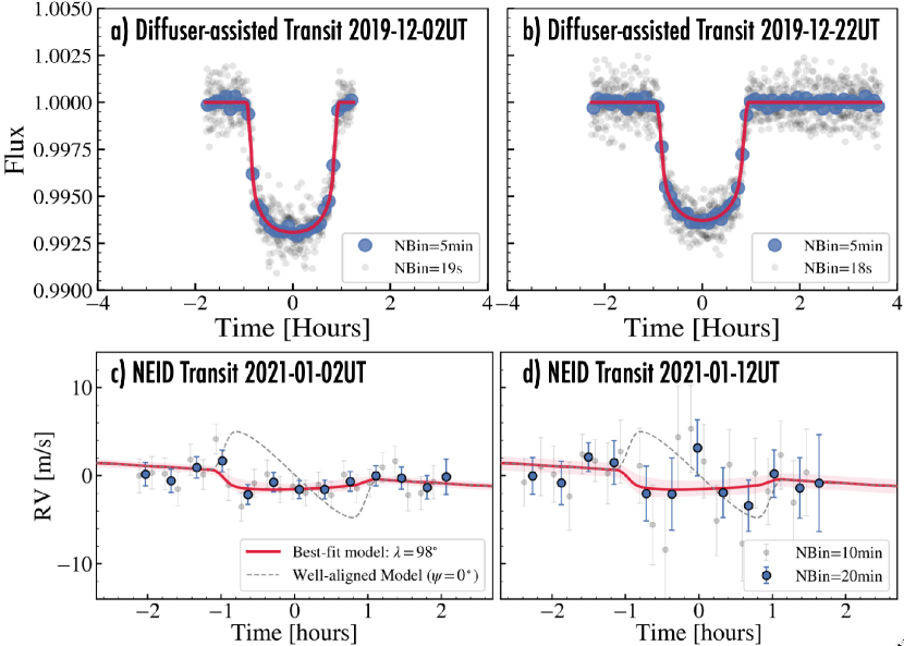
Figure 1: Top panels: Diffuser-assisted transit observations with the ARCTIC imager on the ARC 3.5m Telescope at Apache Point Observatory on (a) 2 December 2019, and (b) 22 December 2019. The best fit model is shown in red, unbinned data are shown in black, and 5-min binned data are shown with the blue points. Lower panels: RM effect of GJ 3470b as observed by NEID on c) 2 January 2021 UT, and d) 12 January 2021 UT. The best-fit joint model of both RM observations (red) results in a sky-projected obliquity of $\lambda=98_{-12}^{+15\>\circ}$. The red regions show the $1\sigma$ credible intervals. The expected well-aligned model is shown with the grey-dashed lines, which assumes $\psi=0^{\circ}$, i.e., that $v\sin i=v_{\mathrm{eq}}$, and $\lambda=0^{\circ}$. Both observations disfavor the well-aligned model. The RVs and diffuser-assisted photometry are available as data behind the figure.

To extract the RVs, we used a customized version of the Spectrum Radial Velocity Analyzer (SERVAL) pipeline (Zechmeister et al., 2018) optimized for NEID spectra, which uses the template-matching method to extract precise RVs. This version of the code is based both on the original SERVAL code by Zechmeister et al. (2018) as well as the customized version for the Habitable-zone Planet Finder (HPF) instrument by Stefansson et al. (2020a). We verified during NEID commissioning that when applied to the spectra of many reference stars, the SERVAL template-matching RVs are consistent with the official version of the NEID pipeline, which derives precise RVs using the cross-correlation method. However, the template-matching method is capable of using a higher fraction of the rich information content inherent in spectra of M dwarfs such as GJ 3470, resulting in higher precision RVs.

As this was the first time we used this implementation of SERVAL for NEID data, we provide more details here. To extract precise RVs, we used order indices 30-104 spanning the wavelength region from 426 nm to 895 nm. Although NEID is sensitive down to 380 nm, the bluer orders had very low SNR given the faintness of GJ 3470 at blue wavelengths, and including those orders did not improve the resulting RV uncertainties. Barycentric corrections were calculated using the barycorrpy package (Kanodia & Wright, 2018), which uses the algorithms from Wright & Eastman (2014). To mask out telluric lines, we used the synthetic telluric mask calculated using the TERRASPEC code (Bender et al., 2012), an IDL wrapper to the Line-By-Line Radiative Transfer Model package (Clough et al., 2005). We calculated the mask using parameters applicable for NEID’s location on Earth, and nominal assumptions about humidity. We used this synthetic telluric spectrum to generate a thresholded binary mask. Any telluric line deeper than 0.5% was masked. After generating the thresholded mask, we further broadened the mask by 21 wavelength resolution elements to conservatively mask telluric contaminated regions. We experimented with using the NEID sky fiber to subtract the background sky from the science fiber, but this did not significantly change the RVs. As we obtained a slightly higher RV precision without performing the sky-subtraction, we elected to extract the RVs from non-sky subtracted spectra.

3.2 Diffuser-assisted Photometry

To refine the transit ephemeris, we observed two photometric transits of GJ 3470b using the Astrophysical Research Council Telescope Imaging Camera (ARCTIC; Huehnerhoff et al., 2016) on the ARC 3.5m Telescope at Apache Point Observatory in New Mexico. The two nights were 2019 December 2 and 22 UT. We used the Engineered Diffuser available on the ARCTIC imager (Stefansson et al., 2017) because it enables high precision photometry by molding the point-spread function into a broad and stabilized top-hat shape. To minimize atmospheric systematics, we used a narrow-band (30 nm wide) filter from Semrock Optics which is centered in a region with minimal telluric absorption at 857 nm (for further details, see Stefansson et al. 2017 and Stefansson et al. 2018). The mean cadence was 19.1 s and 18.2 s for the two transits respectively. Both observations used ARCTIC’s 2x2 binning mode, which has a gain of $2.0\,\mathrm{e/ADU}$ and a plate scale of $0.22\,\mathrm{\arcsec/pixel}$.

We bias corrected and flat fielded the data using standard procedures described by Stefansson et al. (2017). To extract the photometry, we used AstroImageJ (Collins et al., 2017), following the methodology of Stefansson et al. (2017). We tried several different aperture sizes and ultimately adopted an aperture radius of 27 pixels and 34 pixels for the December 2 and 22 observations, respectively, which showed the lowest standard deviation in the transit residuals. For both observations, the background level was estimated from the counts within an annulus ranging from 60 to 90 pixels in radius. We estimated the uncertainty in each photometric measurement as the standard uncertainty from AstroImageJ accounting for photon, read, dark, and and digitization noise added in quadrature to our independent estimate of the scintillation noise following the methodology in Stefansson et al. (2017). The transits are shown in Figure 1.

3.3 Out-of-transit Spectroscopy

In addition to the in-transit spectroscopy with NEID, we analyzed out-of-transit RVs to constrain the possibility of an outer companion. For this analysis, we used RVs from the High Resolution Echelle Spectrometer (HIRES; Vogt et al., 1994) on the Keck I telescope on Maunakea, the HARPS spectrograph (Mayor et al., 2003) on the 3.6m Telescope at La Silla Observatory in Chile, and the Habitable-zone Planet Finder (HPF) spectrograph (Mahadevan et al., 2012, 2014) on the 10m Hobby-Eberly Telescope in Texas.

For HIRES, we used precise RVs derived with the iodine technique as published by Kosiarek et al. (2019), totalling 56 RV points with a median RV precision of 1.89m/s.

For HARPS, we note that Kosiarek et al. (2019) analyzed RVs from HARPS from 2008 December to 2017 April including data from the original GJ 3470b discovery paper from Bonfils et al. (2012). In addition to the data analyzed in Kosiarek et al. (2019), we noticed that 6 additional RVs were publicly available on the HARPS archive obtained in 2018 March and April as part of program 198.C-0838(A) (PI: Bonfils). As these additional RVs extended the HARPS baseline by a year, we downloaded all of the available HARPS data from the HARPS archive, and extracted precise radial velocities using SERVAL. We removed one point as clear low S/N outlier, leaving 122 HARPS points with a median RV precision of 2.85m/s. We also used SERVAL to extract the H$\alpha$ activity index, and we extracted the Ca II H&K $S_{\mathrm{HK}}$ index values from the HARPS spectra following Gomes da Silva et al. (2011) and Robertson et al. (2016).

Additionally, we used near-infrared out-of-transit RVs obtained with the Habitable-zone Planet Finder (HPF) spectrograph. HPF is a fiber-fed near-infrared (NIR) spectrograph on the 10m Hobby-Eberly Telescope (Mahadevan et al., 2012, 2014) at McDonald Observatory in Texas, covering the $z$, $Y$, and $J$ bands from 810$\,\mathrm{nm}$-1260$\,\mathrm{nm}$ at a resolution of $R\sim 55,000$. To enable precision radial velocities in the NIR, HPF is temperature stabilized at the milli-Kelvin level (Stefansson et al., 2016). A subset of the HPF spectra were originally discussed by Ninan et al. (2020) to demonstrate that GJ 3470b shows an absorption in the He 10830Å line during transit. To avoid the complexity of modeling the RM effect, we only considered HPF data that were not obtained during transits. This resulted in 9 observations with a median RV precision of 4.5m/s. The HPF 1D spectra were reduced using the HPF pipeline following the procedures in Ninan et al. (2018), Kaplan et al. (2018), and Metcalf et al. (2019). Following the 1D spectral extraction, we reduced the HPF radial velocities using a version of the SERVAL template-matching RV-extraction pipeline (Zechmeister et al., 2018) optimized for HPF RV extractions, which is described in Stefansson et al. (2020a). Following Stefansson et al. (2020a), we only use the 8 HPF orders that are cleanest of tellurics, covering the wavelength regions from 8540-8890Å, and 9940-10760Å. We subtracted the estimated sky-background from the stellar spectrum using the dedicated HPF sky fiber, and we masked out telluric lines and sky-emission lines to minimize their impact on the RV determination.

Together the available RV data from HIRES, HARPS, and HPF span a baseline of 4709 days, or about 12.9 years from 2008 December 7 to 2021 October 29.

4 Transit Ephemeris

To update the orbital ephemeris of GJ 3470b, we used a two-step procedure. First, we modeled the two ARCTIC transits independently to obtain precise transit midpoints for each transit. To model the transits, we followed the methodology of Stefansson et al. (2020b) using the juliet code (Espinoza et al., 2019). juliet uses the batman code (Kreidberg, 2015) for the transit model and the dynesty dynamic nested sampler (Speagle, 2020) to perform a dynamic nested sampling of the posteriors. For the transit model, we placed broad uniform priors on the transit parameters $R_{p}/R_{\star}$, $a/R_{\star}$, and $b$. We sampled the limb darkening parameters using the quadratic $q_{1}$ and $q_{2}$ limb-darkening parameterization of Kipping (2013) with uniform priors. To obtain a constraint on the transit midpoint, we placed a Gaussian prior on the period of the planet based on the value reported by Nascimbeni et al. (2013), and a broad uniform prior on the transit midpoint. To account for correlated noise observed in the light curves, we used a Matern-3/2 Gaussian Process (GP) kernel implemented in celerite (Foreman-Mackey et al., 2017) as available in the juliet code, placing broad uninformative priors on the GP hyperparameters. Figure 1 shows the two transits along with the best-fit models. The transit midpoints (in the $\,\mathrm{BJD_{TDB}}$ system) are $T_{C1}=2458819.85859\pm 0.00025$ and $T_{C2}=2458839.87824\pm 0.00045$.

Second, to update the transit ephemeris, we fitted a linear function of epoch number,

$$T_{C}=nP+T_{0},$$ (1)

to the transit midpoints from ARCTIC and the transit midpoint from Nascimbeni et al. (2013). The results were $P=3.33665266\pm 0.00000030\,\mathrm{days}$, and $T_{0}=2456340.725588\pm 0.00010\,\mathrm{BJD_{TDB}}$. These observations led to an improvement in the precision of the period measurement by a factor of 5, translating to an uncertainty in the transit midpoint of only 0.5 min for the nights of the two NEID spectroscopic observations.

5 Out of Transit RVs

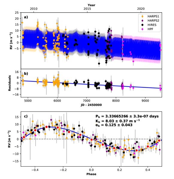
Figure 2: Fit of out-of-transit RVs of GJ 3470 with the known orbit of GJ 3470b, a linear slope, and a quasi-periodic GP model. HARPS RVs before and after the 2015 fiber break are shown in yellow (denoted HARPS1) and purple (denoted HARPS2), respectively, HIRES RVs are shown in black, and HPF RVs in pink. a) RVs as a function of time. b) Residuals including the RV slope. c) Phase-folded RVs. The RVs are available as machine readable data behind the figure.

5.1 RV Fit

To precisely constrain the parameters of GJ 3470b and to probe for any evidence of an outer long-term companion, we modeled the available out-of-transit RVs of GJ 3470 from HARPS, HIRES, and HPF. We fit the RVs using the radvel code (Fulton et al., 2018).

Table 2: Summary of out-of-transit RV fits.

Fit	Slope (m/s/day)	BIC	$\Delta$BIC	AIC	$\Delta$AIC
Model I: No Slope, no GP	-	1129.9	0.0	1090.0	0.0
Model II: Slope, no GP	$-0.0023\pm 0.00069$	1123.7	-6.2	1080.9	-9.1
Model III: No Slope, GP	-	1124.0	-6.0	1072.6	-17.4
Model IV: Slope, GP	$-0.0022\pm 0.0011$	1124.6	-5.4	1070.5	-19.6

To assess the statistical significance of a possible RV slope and quantify the need for using a Gaussian Process (GP) red-noise model to account for stellar activity signatures in the overall RV dataset, we performed a total of four fits with and without RV slopes and with and without a GP model:

• Model I: No Slope, no GP,

• Model II: Slope, no GP,

• Model III: No Slope, GP,

• Model IV: Slope, GP.

These models are summarized in Table 2. For all fits, we placed Gaussian priors on the orbital period ($P$) and transit midpoint ($T_{c}$) from our derived ephemeris in Section 4, a Gaussian prior on the $e\cos\omega=0.014546_{-0.000659}^{+0.000753}$ from Kosiarek et al. (2019) which was derived from the timing of Spitzer secondary eclipse measurements presented by Benneke et al. (2019). We placed uniform priors on the RV semi-amplitude ($K$). The HARPS fiber link was upgraded from circular to octagonal fibers on 2015 May 28 which introduced a zero-point offset in the RV timeseries (Lo Curto et al., 2015). To account for this offset, we modeled the HARPS RVs as two separate RV streams. We include independent RV offset and instrument jitter parameters for each dataset (HARPS before upgrade, HARPS after upgrade, HIRES and HPF). Following the procedures in the radvel package, we first obtained the global maximum likelihood solution, and then sampled the posteriors surrounding the maximum likelihood solution using the emcee affine-invariant Markov Chain Monte Carlo (MCMC) sampler (Foreman-Mackey et al., 2013). We used the default MCMC convergence criteria within the radvel package: convergence is reached when the Gelman-Rubin statistic is less than 1.01 and that the number of independent samples is greater than 1000 for all free parameters.

Table 3: Summary of priors and resulting posteriors for the out-of-transit RV analysis. $\mathcal{N}(m,\sigma)$ denotes a normal prior with mean $m$, and standard deviation $\sigma$; $\mathcal{J}(a,b)$ denotes a Jeffreys prior with a start value $a$ and end value $b$. .

Parameter	Description	Prior	Posterior
MCMC Input Parameters:
$T_{C}$ $(\mathrm{BJD_{TDB}})$	Transit midpoint	$\mathcal{N}(2456340.72559,0.00010)$a	$2456340.72559_{-0.0001}^{+0.00011}$
$P$	Orbital period (days)	$\mathcal{N}(3.33665267,0.00000032)$a	$3.33665266_{-0.0000003}^{+0.0000003}$
$e\cos(\omega)$	Eccentricity and Argument of periastron	$\mathcal{N}(0.014546,0.0007)$b	$0.01444_{-0.00074}^{+0.00074}$
$e\sin(\omega)$	Eccentricity and Argument of periastron	-	$-0.125_{-0.043}^{+0.043}$
$K$	RV semi-amplitude (m/s)	-	$8.03_{-0.37}^{+0.38}$
$\dot{\gamma}$	RV slope (m/s/day)	-	$-0.0022_{-0.0011}^{+0.0011}$
$\gamma_{\mathrm{HIRES}}$	HIRES RV offset (m/s)	-	$2.0_{-1.3}^{+1.3}$
$\gamma_{\mathrm{HARPS1}}$	HARPS RV offset before fiber upgrade (m/s)	-	$-0.11_{-0.89}^{+0.83}$
$\gamma_{\mathrm{HARPS2}}$	HARPS RV offset after fiber upgrade (m/s)	-	$-1.0_{-2.1}^{+2.1}$
$\gamma_{\mathrm{HPF}}$	HPF RV offset (m/s)	-	$6.5_{-3.4}^{+3.6}$
$\sigma_{\mathrm{HIRES}}$	HIRES RV Jitter (m/s)	$\mathcal{J}(0.01,10)$	$2.07_{-0.76}^{+0.67}$
$\sigma_{\mathrm{HARPS1}}$	HARPS RV Jitter before fiber upgrade (m/s)	$\mathcal{J}(0.01,10)$	$0.027_{-0.014}^{+0.056}$
$\sigma_{\mathrm{HARPS2}}$	HARPS RV Jitter after fiber upgrade (m/s)	$\mathcal{J}(0.01,10)$	$0.03_{-0.016}^{+0.073}$
$\sigma_{\mathrm{HPF}}$	HPF RV Jitter (m/s)	$\mathcal{J}(0.01,10)$	$0.028_{-0.014}^{+0.060}$
$\eta_{1}$	GP amplitude (m/s)	$\mathcal{J}(0.01,100)$	$2.92_{-0.43}^{+0.47}$
$\eta_{2}$	GP periodicity (days)	$\mathcal{N}(21.54,0.49)$c	$21.64_{-0.43}^{+0.45}$
$\eta_{3}$	GP exponential length scale	$\mathcal{N}(49,8)$c	$50.1_{-8.0}^{+8.1}$
$\eta_{4}$	GP periodicity length scale (days)	$\mathcal{N}(0.55,0.06)$c	$0.548_{-0.057}^{+0.058}$
Derived Parameters:
$e$	Eccentricity	-	$0.125_{-0.042}^{+0.043}$
$\omega$	Argument of Periastron (deg)	-	$-83.4_{-1.7}^{+3.4}$
$m_{b}\sin i$	Mass of GJ 3470b ($M_{\oplus}$)	-	$12.14_{-0.66}^{+0.68}$

For the fits with an RV slope parameter, we placed no prior on the slope. For fits using a GP, we used the quasi-periodic GP kernel as implemented in the george package (Ambikasaran et al., 2015) available in radvel. This GP kernel has four hyper parameters: the GP RV amplitude $\eta_{1}$, a periodicity parameter $\eta_{2}$, length scale of the exponential component $\eta_{3}$, and a length scale of the periodic component $\eta_{4}$. We follow Kosiarek et al. (2019), and we placed Gaussian priors on $\eta_{2}=49.0\pm 8.0$, $\eta_{3}=21.54\pm 0.49\,\mathrm{days}$, and $\eta_{4}=0.55\pm 0.06$, using the values from Kosiarek et al. (2019) which they constrained by modeling photometric data from Fairborn Observatory. We placed a uniform prior on the GP amplitude.

Table 2 compares the Bayesian Information Criterion (BIC), and the Aikake Information Criterion (AIC) for the four fits we considered. Both the BIC and AIC measure model likelihood while penalizing a higher number of free parameters, where the AIC is less punative toward the number of free parameters. From Table 2, we see that Models II, III and IV are significantly favored over Model I with $\Delta\mathrm{BIC}\geq 5.4$ and $\Delta\mathrm{AIC}\geq 9.1$ in favor of Models II, III and IV. We see that the two models that have a slope (Model II and IV) yield consistent slope values of $\dot{\gamma}=-0.0023\pm 0.00069\,\mathrm{m/s/day}$ and $\dot{\gamma}=-0.0022\pm 0.0011\,\mathrm{m/s/day}$. From Table 2 we see that Models II, III and IV all have similar BIC values within $\Delta\mathrm{BIC}\sim 0.9$ of each other, suggesting they are statistically indistinguishable. The simplest of these models, Model II with a Keplerian and a simple slope, is a good description of the data. We further note that the AIC—which penalizes for additional fitting parameters to a lesser extent than the BIC—favors models with the GP included (Models III and IV). As there are independent evidence of stellar activity from the RVs directly (see discussion in Kosiarek et al. 2019 and in Section 5.2), fits that include a GP stellar activity model are warranted. As the AIC is the lowest for Model IV, which explicitly accounts for a long-term RV slope and signatures of stellar activity, we formally adopt those values, which suggest the data are compatible with an RV slope with $\dot{\gamma}=-0.0022\pm 0.0011\,\mathrm{m/s/day}$, suggesting a detection of a long-term RV slope at $2\sigma$ confidence. We urge additional RV follow-up to confirm or refute this candidate RV slope.

Figure 2 shows the resulting RV fit from Model IV, along with the phase-folded RVs, and Table 3 summarizes the priors and the resulting posteriors. We obtain a semi-amplitude of $8.03_{-0.37}^{+0.38}\,\mathrm{m/s}$ which is consistent with the semi-amplitude of $K=8.21_{-0.46}^{+0.47}\,\mathrm{m/s}$ reported by Kosiarek et al. (2019).

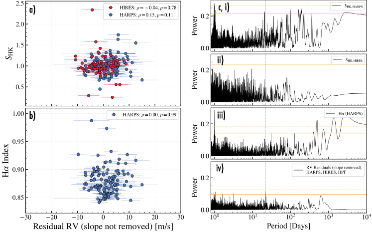
Figure 3: a) $S_{\mathrm{HK}}$ as a function of the residual radial velocity from Model II. The residual RV includes the RV slope (see Figure 2b). b) H$\alpha$ index as a function of residual RV. The Spearman’s rank correlation coefficient $\rho$ for each dataset is shown in the legends. We see no clear correlations with $S_{\mathrm{HK}}$ or H$\alpha$ with the residual RVs. c) Lomb-Scargle periodograms of i) the $S_{\mathrm{HK}}$ indicator from HARPS, ii) $S_{\mathrm{HK}}$ indicator from HIRES, iii) H$\alpha$ indicator from HARPS, iv) residual RV (slope removed) from HARPS, HIRES and HPF. The known stellar rotation period is shown with the red dashed line. The orange horizontal lines show the 10% (solid line) and the 1% (dot-dashed line) false alarm probabilities calculated with the bootstrap method.

5.2 Stellar Activity Correlations

To investigate if stellar activity could account for the long-term RV slope, we studied both the Mount Wilson $S_{\mathrm{HK}}$ index, which traces the chromospheric emission in the cores of the Ca II H&K lines (Vaughan et al., 1978), and the H$\alpha$ index as calculated by the SERVAL pipeline which probes the emission of the H$\alpha$ line. Figure 3a and b) show the $S_{\mathrm{HK}}$ and H$\alpha$ indices as a function of the residual radial velocities from Model II before taking out the long-term RV slope. We show the residual RVs from Model II, as that model does not use a GP that could potentially remove long-term stellar activity activity effects seen in the RVs. The Spearman’s rank correlation coefficient between the residual RVs and the $S_{\mathrm{HK}}$ values is $\rho_{\mathrm{HIRES}}=-0.04$ and $\rho_{\mathrm{HARPS}}=0.15$ with $p$ values $p=0.78$ and $p=0.11$ for the HIRES and HARPS data, respectively. The Spearman’s rank correlation coefficient between the H$\alpha$ index and the HARPS residual RVs is $\rho=0.0$ with $p=0.99$. We see that all cases suggest there is no correlation between the activity indices and the the residual RVs including the RV slope, disfavoring a stellar-activity origin for the long-term RV slope.

To investigate activity signatures at shorter timescales, in particular at the known stellar rotation period, Figure 3 shows Generalized Lomb-Scargle periodograms of the $S_{\mathrm{HK}}$ and H$\alpha$ activity indicators as well as the residual RVs after removing the RV slope from Model II. We see peaks close to the known stellar rotation period in the $S_{\mathrm{HK}}$ index in HARPS (Figure 3c-i), and in the RV residuals (Figure 3c-iv) with false alarm probabilities $\leq 10\%$. Similar peaks in the RV residuals at the stellar rotation period were noted by Kosiarek et al. (2019), suggesting that they originate from stellar active regions. We conclude similar to Kosiarek et al. (2019) that this further motivates the use of a GP model to account for this impact in the RVs. From the parameters from Model IV in Table 3, we see that the best-fit GP amplitude is $3.0\pm 0.5\,\mathrm{m/s}$.

Table 4: Summary of priors and resulting posteriors for the RM analysis. $\mathcal{N}(m,\sigma)$ denotes a normal prior with mean $m$, and standard deviation $\sigma$; $\mathcal{U}(a,b)$ denotes a uniform prior with a start value $a$ and end value $b$..

Parameter	Description	Prior	Posterior	Notes   .
MCMC Input Parameters:
$T_{C}$ $(\mathrm{BJD_{TDB}})$	Transit midpoint	$\mathcal{N}(2456340.72559,0.00010)$	$2456340.725592_{-0.00010}^{+0.00010}$	This work
$P$	Orbital period (days)	$\mathcal{N}(3.33665267,0.00000032)$	$3.33665267_{-0.0000003}^{+0.0000003}$	This work
$R_{p}/R_{*}$	Radius ratio	$\mathcal{N}(0.07642,0.00037)$	$0.07642_{-0.00036}^{+0.00037}$	Biddle et al. (2014)
$a/R_{*}$	Scaled semi-major axis	$\mathcal{N}(13.94,0.5)$	$13.99_{-0.47}^{+0.47}$	Biddle et al. (2014)
$i$	Transit inclination (∘)	$\mathcal{N}(88.88,0.5)$	$88.86_{-0.42}^{+0.38}$	Biddle et al. (2014)
$e$	Eccentricity	$\mathcal{N}(0.125,0.042)$	$0.123_{-0.040}^{+0.040}$	This work
$\omega$	Argument of periastron (∘)	$\mathcal{N}(-83.4,3)$	$-83_{-3}^{+3}$	This work
$K$	RV semi-amplitude (m/s)	$\mathcal{N}(8.0,0.37)$	$7.98_{-0.36}^{+0.37}$	This work
$\gamma_{1}$	NEID RV offset Transit 1 (m/s)	$\mathcal{U}(-100,100)$	$0.5_{-0.45}^{+0.44}$	This work
$\gamma_{2}$	NEID RV offset Transit 2 (m/s)	$\mathcal{U}(-100,100)$	$-0.39_{-0.78}^{+0.78}$	This work
$u_{1}$	Linear limb darkening parameter	$\mathcal{N}(0.35,0.1)$	$0.347_{-0.10}^{+0.099}$	This work
$u_{2}$	Quadratic limb darkening parameter	$\mathcal{N}(0.32,0.05)$	$0.321_{-0.051}^{+0.050}$	This work
$\beta$	Intrinsic stellar line width (km/s)	$\mathcal{N}(3.0,0.5)$	$3.0_{-0.5}^{+0.5}$	This work
$\lambda$	Sky-projected obliquity (deg)	$\mathcal{U}(-180,180)$	$98_{-12}^{+15}$	This work
$R_{\star}$	Radius of star	$\mathcal{N}(0.5,0.016)$	$0.499_{-0.016}^{+0.016}$	This work
$P_{rot}$	Stellar rotation period (days)	$\mathcal{N}(21.54,0.49)$	$21.56_{-0.49}^{+0.49}$	This work
$\cos i$	Cosine of Stellar inclination	$\mathcal{U}(0,1)$	$0.69_{-0.40}^{+0.21}$	This work
Derived Parameters:
$v\sin i$	Projected Rotational Velocity (km/s)	-	$0.85_{-0.33}^{+0.27}$	This work
$i_{\star}$	Stellar inclination (deg)	-	$46_{-20}^{+27}$	This work
$\psi$	True Obliquity (deg)	-	$95_{-8}^{+9}$	This work

6 RM Effect

To model the RM effect observations, we broadly followed the methodology of Stefansson et al. (2020b), which we have implemented in a code named rmfit. In short, we use the RM effect model framework from Hirano et al. (2011b) along with the radvel code (Fulton et al., 2018) to account for the orbital motion of the planet during the transit. We jointly modeled both NEID transits. We placed Gaussian priors on the planet parameters which have been precisely constrained from other observations, and we placed informative priors on the ephemeris derived in Section 4. We place broad uniform priors on $\lambda$. To constrain the true obliquity, we additionally sample the stellar inclination ($i_{\star}$), the stellar radius ($R_{\star}$), and the stellar rotation period ($P_{\mathrm{rot}}$). We place Gaussian priors on the known stellar radius and rotation period to calculate the equatorial velocity of the star, $v_{\mathrm{eq}}$, and we sample the stellar inclination sampled as $\cos i_{\star}$ with a uniform prior on $\cos i_{\star}$. We then estimate the $v\sin i=v_{\mathrm{eq}}\sin i_{\star}=v_{\mathrm{eq}}\sqrt{1-\cos^{2}i_{\star}}$. This broadly follows the methodology in Masuda & Winn (2020), to account for the fact that $v\sin i$ and $v_{\mathrm{eq}}$ are not independent variables (e.g., $v\sin i$ is always lower than $v_{\mathrm{eq}}$). To calculate the true obliquity $\psi$, we used the geometric relation,

$$\cos\psi=\sin i_{\star}\cos\lambda\sin i+\cos i_{\star}\cos i,$$ (2)

where $i_{\star}$ is the stellar inclination, $i$ is the orbital inclination, and $\lambda$ is the sky-projected obliquity.

To account for any possible systematics on timescales longer than one night, we allowed for a separate RV offset for each transit. We placed informative priors on the limb-darkening parameters corresponding to the expected range for the $R$ and $I$-band, where the bulk of the RV information content is located for these observations. We assumed a quadratic limb-darkening law. To account for the finite exposure times of our RV observations, we super-sampled the model with 86-second sampling (7-fold sampling) and averaged the model into 600-seconds bins before comparing the model to the data. We set the intrinsic line width $\beta$ to the width of the NEID resolution element, i.e., $\beta=3.0\pm 0.5\,\mathrm{km/s}$, where the uncertainty is meant to account for any effects of macroturbulence or other processes that could broaden the line profile. For the RM fit, we ignore any effects of stellar activity due to the short duration of the transit compared to the stellar rotation period.

Before MCMC sampling, we first obtained a global maximum-likelihood solution using the using the PyDE differential evolution optimizer (Parviainen, 2016). We then initialized 60 MCMC walkers in the vicinity of the global most probable solution using the emcee MCMC affine-invariant sampling package (Foreman-Mackey et al., 2013). We ran the 60 walkers for 50,000 steps. The mean integrated correlation time for the parameters was 330, suggesting the 50,000 MCMC steps should be sufficiently sampling the posterior distribution. Further, after removing the first 2,000 burn-in steps, the Gelman-Rubin statistic of the resulting chains was within $1\%$ of unity, which we consider well-mixed. Table 4 summarizes the priors and resulting posteriors.

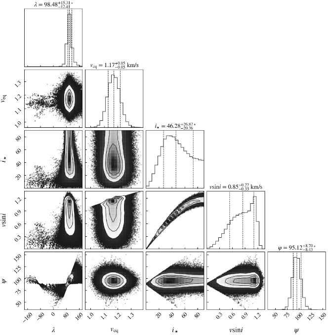
Figure 4: Corner plot of the posteriors of $\lambda$, $v_{\mathrm{eq}}$, $i_{\star}$, $v\sin i$, and $\psi$. The posteriors for the true obliquity are $\psi=95_{-8}^{+9\>\circ}$, and are compatible with $90^{\circ}$ for any posterior value of $v\sin i$.

Figure 1b and c shows the RM effect observations along with the best-fit model (red) which yields a sky-projected obliquity of $\lambda=98_{-12}^{+15\>\circ}$, $v\sin i=0.85_{-0.33}^{+0.27}\,\mathrm{km/s}$, stellar inclination of $i_{\star}=46_{-20}^{+27\>\circ}$, and a true obliquity of $\psi=95_{-8}^{+9\>\circ}$. Figure 4 shows a corner plot of the posteriors, which shows that for any values of $v\sin i$, the true obliquity is robustly $\sim$90^∘, suggesting a polar orbit. From the posteriors, it is valuable to examine Figure 4 in the limit of low and high values of $v\sin i$:

• High values of $v\sin i$: In this case, $v\sin i\sim v_{\mathrm{eq}}$, which represents the highest posterior probability solution as we see from Figure 4. In this limit, we see that for the highest values of $v\sin i$, both $\lambda$ and $\psi$ are confidently $\sim$90^∘. As an additional comparison, in Figure 1, we compare the best-fit RM model in red to the expected well-aligned model in gray which assumes $\psi=0^{\circ}$ (i.e., where we fix $\lambda=0^{\circ}$ and $v\sin i=v_{\mathrm{eq}}$). The Bayesian Information Criterion (BIC) for the best-fit model is $\mathrm{BIC}=44.5$ with 44 degrees of freedom. The BIC for the well-aligned model is $\mathrm{BIC}=103.1$ with 46 degrees of freedom. The resulting $\Delta$BIC = 58.6 strongly disfavors the well-aligned model relative to the best-fit model.

• Low values of $v\sin i$: From Figure 4 we see that although the posterior probability of $v\sin i$ vanishes at $0\,\mathrm{km/s}$, $v\sin i$ is still compatible with low $v\sin i$ values of a few hundred m/s. For such low $v\sin i$ values, we see that the constraint on $\lambda$ becomes poorer. However, as $v\sin i$ decreases, $i_{\star}$ has to decrease accordingly which in turn maintains $\psi\sim 90^{\circ}$. The posteriors show that in the limit of the lowest $v\sin i$ values, $\psi$ becomes even more tightly constrained to $90^{\circ}$ than at higher values of $v\sin i$.

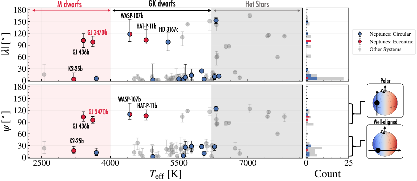
Figure 5: Polar Neptunes: Sky-projected obliquities ($\lambda$; upper panel) and true obliquities ($\psi$; lower panel; when available) as a function of stellar effective temperature. Planets either similar in radius or mass to Neptune ($1.5R_{\oplus}<R<6R_{\oplus}$ or $10M_{\oplus}<M<50M_{\oplus}$) on circular orbits are highlighted in blue, and Neptunes on eccentric orbits ($e>0.1$ and >2$\sigma$ discrepant from $e=0$) are shown in red. Other systems from Albrecht et al. (2021) are shown in grey. We show WASP-107b as both red and blue, as it formally has an eccentricity constraint of $e=0.06\pm 0.04$ and Piaulet et al. (2021) mention it could have a moderate eccentricity. GJ 3470b joins a growing sample of warm Neptunes orbiting cool stars on polar orbits. Data obtained from Albrecht et al. (2021), TEPCAT (Southworth, 2011), and the NASA Exoplanet archive (Akeson et al., 2013).

To test the robustness of the results, we performed three additional tests. First, we tried placing a uniform prior on the semi-amplitude $K$ of the planet from 0 to 25m/s instead of an informative prior. This resulted in fully consistent results to those presented in Table 4. Second, we performed a separate RM fit where we only fit the parameters that are primarily constrained by the RM curve ($\lambda$, $v\sin i$, and the two RV offsets), while keeping the other values fixed to their median best-fit values or most likely prior values. This also resulted in fully consistent parameters with those presented in Table 4. Third, we also tried a fit with a uniform prior on the $v\sin i$, which yielded fully consistent parameters. Lastly, we experimented fitting the two transits separately, which yielded fully consistent parameters although with lower significance. We adopt the posteriors from the joint fit, as that fit leverages information from both transit observations.

7 Discussion

7.1 Neptunes in Eccentric Polar Orbits around Cool Stars

Recently, Albrecht et al. (2021) noticed that the planets with projected obliquities larger than about $40^{\circ}$ show an apparent preference for polar orbits ($\psi=80-125^{\circ})$ rather than spanning the full range of possible obliquities. Most of the polar systems involve hot Jupiters ($R>6R_{\oplus}$ and $P<10$ days) because the RM measurements of smaller and longer-period planets are more difficult.

Among the sample from Albrecht et al. (2021) is a collection of four warm Neptunes ($a/R_{\star}\gtrsim 8$; $1.5<R_{p}/R_{\oplus}<6$) orbiting cool K and M dwarfs that are observed to be on polar orbits: HAT-P-11b (Winn et al., 2010; Hirano et al., 2011a), GJ 436b (Bourrier et al., 2018a, 2022), HD 3167c (Dalal et al., 2019; Bourrier et al., 2021), and WASP-107b (Dai & Winn, 2017; Rubenzahl et al., 2021). Figure 5 highlights these planets along with obliquity constraints available for other Neptunes. Together with GJ 3470b, we have a sample of five polar warm Neptunes. Four of these planets—GJ 3470b, GJ 436b, HAT-P-11b, and WASP-107b—all reside in or at the edge of the “Neptune Desert” (e.g., Mazeh et al., 2016; Owen & Lai, 2018) and are observed to have evaporating atmospheres. Further, three of these planets have non-circular orbits with eccentricities above 0.1 (GJ 3470b, GJ 436b, and HAT-P-11b), and we note that WASP-107 has an eccentricity constraint of $e=0.06\pm 0.04$ and Piaulet et al. (2021) explicitly mention the planet could have a moderate eccentricity. These similar properties could suggest that these systems share a similar formation history. We discuss possible formation scenarios in Section 7.3.

7.2 Tidal Inflation

It is intriguing to consider possible causal links between the orbital properties of the polar, moderately eccentric Neptunes mentioned above and their atmospheric mass loss. One possibility is that their mass loss is enhanced from atmospheric inflation driven by tidal heating, with the atmosphere being eroded by photoevaporation (see e.g., Owen & Lai, 2018; Attia et al., 2021). Short-period planets experience significant tidal deformations due to their close proximity to their host stars. Whenever the planets have non-zero eccentricities and/or axial tilts (planetary obliquities), these tidal deformations are non-uniform along the orbital path, and they drive interior friction and heat dissipation known as “tidal heating” (e.g., Jackson et al., 2008). This extra interior energy source can significantly inflate the atmospheres of gas-rich planets, as shown in previous works on hot Jupiters (e.g., Bodenheimer et al., 2001; Miller et al., 2009), sub-Neptunes (Millholland, 2019), and sub-Saturns (Millholland et al., 2020).

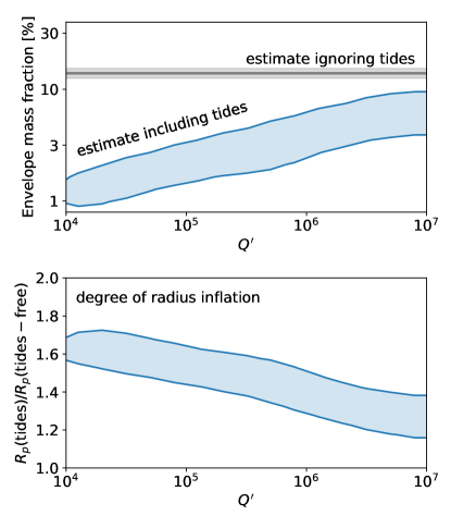
Figure 6: Results from the tidal model fit to the observed properties of GJ 3470b. Top panel: Comparison of the envelope mass fraction ($f_{\mathrm{env}}\equiv M_{\mathrm{env}}/M_{p}$) when tides are included and when they are ignored. The gray solid line and banding indicates the mean and standard deviation of the tides-free estimate, $f_{\mathrm{env}}=14.0\%\pm 1.4\%$. The blue solid region indicates the 2$\sigma$ contours of the posterior distribution of the planet’s reduced tidal quality factor, $Q^{\prime}$, and $f_{\mathrm{env}}$ when accounting for tides. Bottom panel: The degree of radius inflation, parameterized as the ratio of the radius of the planet when tides are accounted for compared to the radius the planet would have if tides were absent. The blue solid region indicates the 2$\sigma$ contours of the posterior distribution. $Q^{\prime}$ is highly uncertain but most likely in the range $Q^{\prime}\approx 10^{4}-10^{5}$, indicating tidal inflation by a factor of $\sim 1.5-1.7$.

As an illustrative example, we can estimate how much GJ 3470b’s atmosphere has been inflated from tidal heating. According to traditional equilibrium tide theory (e.g., Hut, 1981; Leconte et al., 2010), the tidal luminosity—the rate of tidal energy dissipation inside the planet—is approximately $L_{\mathrm{tide}}\approx 4.8\times 10^{25}$ erg/sec, or roughly 4% of the incident stellar power. Here we used the equations of Leconte et al. (2010) assuming zero planetary obliquity and a reduced tidal quality factor, $Q^{\prime}$, equal to $10^{5}$. To quantitatively assess how this tidal luminosity affects the planetary structure, we fit a tidal model utilizing previous simulation results from Millholland (2019) and Millholland et al. (2020). The model consists of a spherically symmetric, two-layer planet containing a heavy element core and a H/He envelope. The thermal evolution of the atmospheric envelope is calculated using the Modules for Experiments in Stellar Astrophysics (MESA; Paxton et al. 2011, 2013) 1D stellar evolution code, including a series of modifications developed by Chen & Rogers (2016) that make the model specific to planets as opposed to stars. Additionally, the model accounts for tidal energy deposited in the planet’s deep atmosphere. The full details of the model are provided in Millholland (2019) and Millholland et al. (2020). Here we use an interpolation to the simulation set developed in Millholland et al. (2020), and we use the Markov Chain Monte Carlo fitting procedure described therein to estimate the planet’s envelope mass fraction ($f_{\mathrm{env}}\equiv M_{\mathrm{env}}/M_{p}$) and degree of tidal radius inflation. We assume that the eccentricity is fixed to $e=0.125$ (Table 3) and that the planetary obliquity is zero.

Figure 6 shows the results of the tidal inflation analysis. The top panel indicates that the estimate of the planet’s envelope mass fraction is much smaller when tides are included in the model compared to when they are ignored. This is because planets with active tidal heating are larger at a fixed $f_{\mathrm{env}}$, so the inclusion of tidal heating in the structural model yields smaller $f_{\mathrm{env}}$ estimates for observed planets. Moreover, smaller values of the planet’s reduced tidal quality factor are associated with smaller values of $f_{\mathrm{env}}$, since the stronger dissipation at smaller $Q^{\prime}$ requires a smaller envelope fraction to match the planet’s observed radius. The bottom panel indicates that GJ 3470b is anywhere between $\sim 1.2-1.7$ times larger than it would be in the absence of tides. However, a tidal quality factor in the range of $Q^{\prime}\approx 10^{4}-10^{5}$ is most reasonable for this size of planet (Millholland et al. 2020 and references therein). Thus, tidal heating has most likely inflated GJ 3470b by a factor of $\sim 1.5-1.7$.

With an inflated atmosphere, GJ 3470b is more susceptible to atmospheric escape than it would be in the absence of tidal heating. Tidal inflation, coupled with photoevaporation, thus serves as a potential connection between the orbital properties of the growing population of polar, eccentric Neptunes and their ongoing mass loss. We suggest future, more detailed studies on this connection.

7.3 Possible Origin of the Polar Orbit

How did GJ 3470b obtain its polar orbit? Different theoretical models have been developed to explain the origin of polar planetary orbits, and here we consider a few possible explanations.

Highly inclined orbits can be produced through a primordial tilt of the protoplanetary disk (Batygin, 2012), requiring interactions with a massive binary stellar companion or a stellar fly-by event (Malmberg et al., 2011). Although we do not know if a stellar fly-by occurred in the system, GJ 3470 is not currently known to be in a stellar binary system. Additionally, polar orbits can be obtained through magnetic disk-torquing from the young magnetized star (Lai et al., 2011). Although a plausible path to misaligning the disk and the orbit of GJ 3470b, this scenario acting alone could not easily explain the non-circular orbit of the planet ($e=0.122_{-0.041}^{+0.042}$).

Other theoretical scenarios that can explain the moderate eccentricity and polar orbit of GJ 3470b demand multi-body dynamical interactions. Among such models is planet-planet scattering (Rasio & Ford, 1996; Chatterjee et al., 2008). However, given the current large orbital velocity of GJ 3470b relative to its current escape speed ($[V_{\rm esc}/V_{\rm orb}]^{2}=0.053$), in-situ scattering is inefficient (Ford et al., 2001; Petrovich et al., 2014), favoring scattering at wider orbits. A possible formation scenario could then involve tidal high-eccentricity migration driven by planet-planet scattering, possibly accompanied by secular interactions via the Von Zeipel-Lidov-Kozai (ZLK) mechanism (e.g., Nagasawa et al., 2008). Such models have been shown to be capable of explaining eccentric and misaligned orbits (see e.g., Bourrier et al., 2018a; Correia et al., 2020), and recently specifically highlighted as a path to creating eccentric polar orbits by Dawson & Albrecht (2021). Additionally, Petrovich et al. (2020) presented a model relying on secular interactions between a massive outer planet and a slowly dissipating protoplanetary disk that is capable of explaining polar and eccentric orbits—and especially so for eccentric warm Neptunes orbiting around slowly rotating cool stars.

Given the tentative detection of an RV slope in Section 5, models that invoke secular dynamical interactions with an outer perturber are appealing. Below, we study two different secular excitation models: interactions from an inclined companion within the ZKL mechanism, and the disk-driven model of Petrovich et al. (2020). We show that both models are capable of explaining the polar orbit of GJ 3470b, and are compatible with the candidate RV slope for certain combinations of orbital distances and masses.

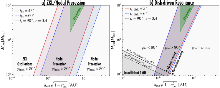
Figure 7: Constraints on the parameters of a potential outer perturber for the two models considered: a) the ZKL/nodal precession model, and b) the disk-driven model of Petrovich et al. (2020). For the former, the red and blue regions show where $\psi_{\rm max}>80^{\circ}$ for $i_{\rm bc}=45^{\circ}$ and $i_{\rm bc}=60^{\circ}$, respectively. For the ZKL/nodal precession case, we assume a current Love number of $k_{2}=0.01$, leading to $J_{2}\sim 2\times 10^{8}$. For the disk-driven model of Petrovich et al. (2020), we assume that GJ 3470 had a radius of $R_{\star}=0.9R_{\odot}$ and rotation period of $10\,\mathrm{days}$ and Love number of $k_{2}=0.2$ during the disk dispersal phase. For this case, we follow Petrovich et al. (2020) and assume a disk mass-loss law of $M_{\mathrm{disk}}=50M_{\rm J}/(1+t/\mathrm{1Myr})^{1/2}$. The grey regions in b) highlight regions excluded from the conservation of angular momentum deficit (AMD). The green regions show the nominal region consistent with the RV slope from Section 5, where we have assumed $i_{c}\leq 90^{\circ}$, $e=0.4$ (the green dashed line shows the $i_{c}=90^{\circ}$ case).

7.4 ZKL Mechanism

Within the ZKL mechanism, a highly inclined companion ’c’ would change the orbital elements of planet b, including its nodal precession, on a timescale

$$\tau_{\mathrm{ZKL}}=\frac{2P_{b}}{3\pi}\left(\frac{b_{c}}{a_{b}}\right)^{3}\frac{M_{\star}}{m_{c}},$$ (3)

which is known as the ZKL timescale (see Kiseleva et al., 1998). Here, $b_{c}=a_{c}(1-e_{c}^{2})^{1/2}$ is the semi-minor axis of the outer companion. This assumes that planet c has a high mutual inclination, which it might have obtained through planet-planet scattering. Due to the close-in orbit of GJ 3470b, general relativistic (GR) precession and the rotationally-induced quadrupole of the host (especially early on its history) may modify the behavior of the ZKL oscillations. Following the notation of Petrovich et al. (2020), we define

$$\eta_{\rm GR}=\frac{8GM_{\star}}{c^{2}}\frac{b_{c}^{3}}{a_{b}^{4}}\frac{M_{\star}}{m_{c}}\simeq 1\left(\frac{1M_{\rm J}}{m_{c}}\right)\left(\frac{b_{c}}{0.4\mbox{AU}}\right)^{3}$$ (4)

and

$$\eta_{\star}=\frac{2J_{2}M_{\star}}{m_{c}}\frac{R_{\star}^{2}b_{c}^{3}}{a_{b}^{5}}\simeq 1\left(\frac{J_{2}}{10^{-6}}\right)\left(\frac{1M_{\rm J}}{m_{c}}\right)\left(\frac{b_{c}}{2\mbox{AU}}\right)^{3}$$ (5)

where $J_{2}$ is the star’s second zonal harmonic. These equations quantify the relative strength of GR corrections and the stellar quadrupole with respect to the two-planet interaction.

The general ZKL mechanism is capable of exciting both eccentricities and inclinations. An accurate treatment of the ZKL mechanism during periods of high-eccentricity oscillations could lead to orbital migration of the inner planet through tidal star-planet interactions during times of closest approach. For the purposes of this paper, we defer an analysis of star-planet tidal interactions to future work. Instead, we highlight the simpler and instructive special case of the ZKL mechanism in the limit where the eccentricity oscillations are quenched by general relativistic precession, resulting in only nodal precession of the inner planet’s orbit. Yee et al. (2018) described this special case of the ZKL mechanism as a possible explanation for the polar orbit of HAT-P-11b, which has a confirmed outer companion HAT-P-11c. As discussed by Fabrycky & Tremaine (2007), eccentricity oscillations are quenched when

$$\sin i_{\rm bc}<\left(\frac{4+\eta_{\rm GR}}{10}\right)^{1/2},$$ (6)

where $i_{\rm bc}$ is the mutual inclination between the planets’ orbits and we have assumed that $\eta_{\rm GR}\gg\eta_{\star}$. The competition between the star’s second zonal harmonic ($J_{2}$) and the possible outer planet orbit defines an equilibrium plane—the so-called Laplace plane—inclined by $i_{\rm eq}(\eta_{\star})$ relative the stellar equator (e.g., Tremaine et al. 2009). Assuming the inner planet starts with zero obliquity, it will precess around the normal to this plane, sweeping out a cone with angle $i_{\rm eq}$ and driving oscillations of the obliquities from 0 to $\psi_{\mathrm{max}}=2i_{\rm eq}$, where

$$\psi_{\rm max}=\tan^{-1}\left[\frac{\sin(2i_{\rm bc})}{\cos(2i_{\rm bc})+\eta_{\star}}\right].$$ (7)

As expected, $\psi_{\rm max}=0$ when $\eta_{\star}\gg 1$ ($J_{2}$-dominated) and $\psi_{\rm max}=2i_{\rm bc}$ for $\eta_{\star}\ll 1$ (companion-dominated), passing through $\psi_{\rm max}=i_{\rm bc}$ at $\eta_{\star}=1$.

In Figure 7a, we show the allowed properties of the outer planet that lead to $\psi_{\rm max}>80^{\circ}$ for two different choices of $i_{\rm bc}$, $45^{\circ}$ and $60^{\circ}$. From Figure 7, we see that the outer companion needs a semi-minor axis $b_{\mathrm{out}}\lesssim 10\,\mathrm{AU}$ to result in $\psi_{\mathrm{max}}>80^{\circ}$. Further, Figure 7a shows that orbits with semi-minor axes between 1 and 10AU experience only nodal precession with no eccentricity oscillations for the inner planet. We also see that for closer-in orbits of $\lesssim 1$AU, such orbits are capable of creating polar orbits for the inner planet but would excite both inclinations and eccentricities of the inner planet, likely leading to orbital migration of the inner planet.

7.5 Disk-Driven Resonance Model

The model of Petrovich et al. (2020) relies on secular interactions between an outer planet and a slowly dissipating protoplanetary disk, allowing for a process of inclination resonance sweeping and capture. In this model the final obliquity becomes

$$\psi=\sin^{-1}\left(\frac{4+4\eta_{\star}+\eta_{\rm GR}}{10+5\eta_{\star}}\right)^{1/2},$$ (8)

for $\eta_{\rm GR}<6+\eta_{\star}$ and $\psi=90^{\circ}$ for $\eta_{\rm GR}>6+\eta_{\star}$. The conditions for the resonance capture are:

1. The presence of a massive disk such that the resonance is encountered (condition in Eq. 2 in Petrovich et al. 2020),

2. The process is adiabatic. This criterion requires the disk dispersal timescale $\tau_{\rm disk}=|d\log M_{\rm disk}/dt|^{-1}$ at crossing to be longer than the adiabatic timescale $\tau_{\rm ad}=\tau_{\rm ZKL}(1+\eta_{\star})^{1/3}/i_{\rm c,disk}^{4/3}$, where $i_{\rm c,disk}$ is the inclination of the outer planet relative to the disk.

Figure 7b graphically shows where the disk-driven model scenario of Petrovich et al. (2020) suggests that polar orbits of GJ 3470b can be obtained. Similarly to the ZKL/nodal precession case in Figure 7a, we see that polar orbits of GJ 3470b can be obtained if a massive perturber (a few Jupiter masses) exists in the system at an orbital distance of $\sim$1-10AU. For the input parameters considered, we note that the disk-driven model case suggests a narrower parameter space where polar orbits can be produced. Similarly to the ZKL/Nodal precession case, we see from Figure 7b that the disk-driven model is also fully consistent with the RV slope (green region) discussed in Section 5.

Lastly, we note that the two models differ in their predictions for the mutual inclination between the inner planet and the outer companion. The ZKL/Nodal Precession case suggests a likely mutual inclination of $\sim$$45-60^{\circ}$, whereas the disk-driven resonance scenario suggests a mutual inclination closer to $90^{\circ}$. Future observations that constrain the orbital properties of the outer planet along with the mutual inclinations between the two planets can help distinguish between the two scenarios.

7.6 Future Constraints on a Possible Outer Companion

A distant outer companion GJ 3470c with the right properties could explain the eccentric and polar orbit of GJ 3470b. Similar explanations were proposed for the polar orbits of GJ 436b, HAT-P-11b, and WASP-107b, the latter two of which have confirmed massive distant companions (see Yee et al. 2018, and Piaulet et al. 2021, respectively). An outer companion in the GJ 436 system has not yet been found (see Bourrier et al. 2018a for observational and theoretical constraints on potential outer companions). The existence of an outer companion GJ 3470c can be further confirmed with additional precise RVs, astrometric measurements from Gaia, and direct imaging observations.

Additional precise radial velocities will be immediately useful in confirming or ruling out the RV slope discussed above, and to see if such a slope starts to curve and reveal a periodicity. From both theoretical models discussed above, to produce polar orbits for the inner planet, we would expect the outer companion to be at a distance of a few AU. If the candidate RV slope discussed in Section 5 is due to an acceleration from an outer companion, Figure 7 shows that both model scenarios considered in the previous subsection are compatible with the slope. If the RV slope is not due to an acceleration due to an outer companion (e.g., stellar activity or other effects) there remains a possibility that a companion could be present in the system but at low inclinations that would not have been detected in the RV datasets.

Additionally, direct imaging would be sensitive to the most massive and distant outer perturbers within the regions in Figure 7. If we assume an orbital distance of $5\,\mathrm{AU}$ (within the green region in Figure 7) the maximum sky-projected planet-star separation is $0.17\,\mathrm{mas}$. Assuming a radius and albedo similar to Jupiter, the reflected-light contrast ratio of the planet is $\sim$$1.5\times 10^{-9}$, and could be a potential but challenging target for future constraints via high-contrast imaging. The Roman Space Telescope is expected to have a $10^{-9}$ effective contrast and $0.140\arcsec$ inner working angle, and may be able to characterize GJ 3470c if it exists. Additionally, we note that JWST MIRI, with an inner working angle of $0.33\arcsec$, could potentially place constraints on orbits beyond 10AU (e.g., Brande et al., 2020).

Lastly, precise astrometric data from Gaia can help constrain the possibility of an outer companion. We note that the Gaia EDR3 astromety (Lindegren et al., 2021) shows that GJ 3470 has an excess astrometric noise of $0.18\,\mathrm{mas}$ with an astrometric excess noise significance of $48\sigma$, which can be a sign of binarity. However, redder stars can also show significant astrometric noise independent of binarity (e.g., Thao et al., 2020). The Gaia Renormalized Unit Weight Error (RUWE) accounts for this color effect and has been shown to be a reliable indicator of binarity (see e.g., Ziegler et al., 2020), where RUWE=1.0 indicates an astrometric solution consistent with a single star, with RUWE values larger than 1 indicative of non-single or extended sources. GJ 3470 has a RUWE=1.14. This value is consistent with a single M-dwarf star (see e.g., Thao et al., 2020) disfavoring a stellar binary, but we can not rule out the possibility of non-stellar companion in the system. Future Gaia releases with access to the intermediate astrometric data products will enable more direct tests to probe for outer companions in the Gaia data. In particular, Sozzetti et al. (2014) calculated the expected fraction of M-dwarfs within 30 pc for which Gaia could detect a giant planet, finding an overall detection efficiency of $\sim$60%, highlighting the possibility that an outer companion could be within the detectability threshold of the Gaia mission.

8 Conclusion and Summary

By observing two transits with the newly commissioned NEID Spectrograph on the WIYN 3.5m Telescope, we showed that the warm Neptune GJ 3470b has a polar orbit with a true obliquity of $\psi=95_{-8}^{+9\>\circ}$. We show that a well-aligned model ($\psi=0^{\circ}$) is strongly disfavored ($\Delta$BIC=58.6) relative to the best-fit misaligned model. This determination was facilitated by an improvement in the transit ephemeris using diffuser-assisted photometry with the ARC 3.5m Telescope at Apache Point Observatory.

GJ 3470b joins a growing sample of warm Neptunes with nearly polar and mildly eccentric orbits, which could hint at the presence of a class of planetary systems that could share common formation histories. Using a tidal inflation model, we show that tidal heating due to GJ 3470b’s mild eccentricity of $e\sim 0.125$ has likely inflated the planet’s radius by a factor of $1.5-1.7$, which can help account for its evaporating atmosphere. The polar and eccentric orbit of GJ 3470b—along with its evaporating atmosphere—together point to a formation scenario involving multi-body dynamical interactions, which likely includes interactions with a massive distant perturber. Using out-of-transit radial velocities spanning 13 years from HARPS, HIRES and HPF, we show that the RV data are compatible with a long-term RV slope at the $\sim$$2\sigma$ level although additional RV observations are needed to confirm or rule out this possible RV slope. Using two different secular excitation models, we constrain the possible orbital locations of an outer companion in the system, and we show that both models are compatible with the candidate RV slope. Future observations could both constrain the presence of an outer companion and further help distinguish between the two different secular excitation models through the measurement of the mutual inclinations between the inner planet and the potential outer companion.

References

- Akeson et al. (2013) Akeson, R. L., Chen, X., Ciardi, D., et al. 2013, PASP, 125, 989, doi: 10.1086/672273
- Albrecht et al. (2012) Albrecht, S., Winn, J. N., Johnson, J. A., et al. 2012, ApJ, 757, 18, doi: 10.1088/0004-637X/757/1/18
- Albrecht et al. (2021) Albrecht, S. H., Marcussen, M. L., Winn, J. N., Dawson, R. I., & Knudstrup, E. 2021, arXiv e-prints, arXiv:2105.09327. https://arxiv.org/abs/2105.09327
- Allart et al. (2018) Allart, R., Bourrier, V., Lovis, C., et al. 2018, Science, 362, 1384, doi: 10.1126/science.aat5879
- Allart et al. (2019) —. 2019, A&A, 623, A58, doi: 10.1051/0004-6361/201834917
- Ambikasaran et al. (2015) Ambikasaran, S., Foreman-Mackey, D., Greengard, L., Hogg, D. W., & O’Neil, M. 2015, IEEE Transactions on Pattern Analysis and Machine Intelligence, 38, 252, doi: 10.1109/TPAMI.2015.2448083
- Astropy Collaboration et al. (2013) Astropy Collaboration, Robitaille, T. P., Tollerud, E. J., et al. 2013, A&A, 558, A33, doi: 10.1051/0004-6361/201322068
- Attia et al. (2021) Attia, O., Bourrier, V., Eggenberger, P., et al. 2021, A&A, 647, A40, doi: 10.1051/0004-6361/202039452
- Bailer-Jones et al. (2018) Bailer-Jones, C. A. L., Rybizki, J., Fouesneau, M., Mantelet, G., & Andrae, R. 2018, AJ, 156, 58, doi: 10.3847/1538-3881/aacb21
- Batygin (2012) Batygin, K. 2012, Nature, 491, 418, doi: 10.1038/nature11560
- Bender et al. (2012) Bender, C. F., Mahadevan, S., Deshpande, R., et al. 2012, ApJ, 751, L31, doi: 10.1088/2041-8205/751/2/L31
- Benneke et al. (2019) Benneke, B., Knutson, H. A., Lothringer, J., et al. 2019, Nature Astronomy, 3, 813, doi: 10.1038/s41550-019-0800-5
- Biddle et al. (2014) Biddle, L. I., Pearson, K. A., Crossfield, I. J. M., et al. 2014, MNRAS, 443, 1810, doi: 10.1093/mnras/stu1199
- Bodenheimer et al. (2001) Bodenheimer, P., Lin, D. N. C., & Mardling, R. A. 2001, ApJ, 548, 466, doi: 10.1086/318667
- Bonfils et al. (2012) Bonfils, X., Gillon, M., Udry, S., et al. 2012, A&A, 546, A27, doi: 10.1051/0004-6361/201219623
- Bourrier et al. (2021) Bourrier, Lovis, C., Cretignier, M., et al. 2021, A&A, 654, A152, doi: 10.1051/0004-6361/202141527
- Bourrier et al. (2018a) Bourrier, V., Lovis, C., Beust, H., et al. 2018a, Nature, 553, 477, doi: 10.1038/nature24677
- Bourrier et al. (2018b) Bourrier, V., Lecavelier des Etangs, A., Ehrenreich, D., et al. 2018b, Astronomy and Astrophysics, 620, A147, doi: 10.1051/0004-6361/201833675
- Bourrier et al. (2022) Bourrier, V., Zapatero Osorio, M. R., Allart, R., et al. 2022, arXiv e-prints, arXiv:2203.06109. https://arxiv.org/abs/2203.06109
- Brande et al. (2020) Brande, J., Barclay, T., Schlieder, J. E., Lopez, E. D., & Quintana, E. V. 2020, AJ, 159, 18, doi: 10.3847/1538-3881/ab5444
- Cegla et al. (2016) Cegla, H. M., Lovis, C., Bourrier, V., et al. 2016, A&A, 588, A127, doi: 10.1051/0004-6361/201527794
- Chatterjee et al. (2008) Chatterjee, S., Ford, E. B., Matsumura, S., & Rasio, F. A. 2008, ApJ, 686, 580, doi: 10.1086/590227
- Chen & Rogers (2016) Chen, H., & Rogers, L. A. 2016, ApJ, 831, 180, doi: 10.3847/0004-637X/831/2/180
- Clough et al. (2005) Clough, S. A., Shephard, M. W., Mlawer, E. J., et al. 2005, J. Quant. Spec. Radiat. Transf., 91, 233, doi: 10.1016/j.jqsrt.2004.05.058
- Collins et al. (2017) Collins, K. A., Kielkopf, J. F., Stassun, K. G., & Hessman, F. V. 2017, AJ, 153, 77, doi: 10.3847/1538-3881/153/2/77
- Correia et al. (2020) Correia, A. C. M., Bourrier, V., & Delisle, J. B. 2020, A&A, 635, A37, doi: 10.1051/0004-6361/201936967
- Dai & Winn (2017) Dai, F., & Winn, J. N. 2017, AJ, 153, 205, doi: 10.3847/1538-3881/aa65d1
- Dalal et al. (2019) Dalal, S., Hébrard, G., Lecavelier des Étangs, A., et al. 2019, A&A, 631, A28, doi: 10.1051/0004-6361/201935944
- Dawson & Albrecht (2021) Dawson, R. I., & Albrecht, S. H. 2021, arXiv e-prints, arXiv:2108.09325. https://arxiv.org/abs/2108.09325
- Dawson & Johnson (2018) Dawson, R. I., & Johnson, J. A. 2018, ARA&A, 56, 175, doi: 10.1146/annurev-astro-081817-051853
- Eastman et al. (2019) Eastman, J. D., Rodriguez, J. E., Agol, E., et al. 2019, arXiv e-prints (submitted to PASP). https://arxiv.org/abs/1907.09480
- Ehrenreich et al. (2015) Ehrenreich, D., Bourrier, V., Wheatley, P. J., et al. 2015, Nature, 522, 459, doi: 10.1038/nature14501
- Espinoza et al. (2019) Espinoza, N., Kossakowski, D., & Brahm, R. 2019, MNRAS, 490, 2262, doi: 10.1093/mnras/stz2688
- Fabrycky & Tremaine (2007) Fabrycky, D., & Tremaine, S. 2007, ApJ, 669, 1298, doi: 10.1086/521702
- Ford et al. (2001) Ford, E. B., Havlickova, M., & Rasio, F. A. 2001, Icarus, 150, 303, doi: 10.1006/icar.2001.6588
- Foreman-Mackey (2016) Foreman-Mackey, D. 2016, JOSS, 24, doi: 10.21105/joss.00024
- Foreman-Mackey et al. (2017) Foreman-Mackey, D., Agol, E., Ambikasaran, S., & Angus, R. 2017, AJ, 154, 220, doi: 10.3847/1538-3881/aa9332
- Foreman-Mackey et al. (2013) Foreman-Mackey, D., Hogg, D. W., Lang, D., & Goodman, J. 2013, PASP, 125, 306, doi: 10.1086/670067
- Fulton et al. (2018) Fulton, B. J., Petigura, E. A., Blunt, S., & Sinukoff, E. 2018, PASP, 130, 044504, doi: 10.1088/1538-3873/aaaaa8
- Gaudi & Winn (2007) Gaudi, B. S., & Winn, J. N. 2007, ApJ, 655, 550, doi: 10.1086/509910
- Ginsburg et al. (2018) Ginsburg, A., Sipocz, B., Parikh, M., et al. 2018, astropy/astroquery: v0.3.7 release, doi: 10.5281/zenodo.1160627
- Gomes da Silva et al. (2011) Gomes da Silva, J., Santos, N. C., Bonfils, X., et al. 2011, A&A, 534, A30, doi: 10.1051/0004-6361/201116971
- Halverson et al. (2016) Halverson, S., Terrien, R., Mahadevan, S., et al. 2016, in Proc. SPIE, Vol. 9908, Ground-based and Airborne Instrumentation for Astronomy VI, 99086P, doi: 10.1117/12.2232761
- Hirano et al. (2011a) Hirano, T., Narita, N., Shporer, A., et al. 2011a, PASJ, 63, 531, doi: 10.1093/pasj/63.sp2.S531
- Hirano et al. (2011b) Hirano, T., Suto, Y., Winn, J. N., et al. 2011b, ApJ, 742, 69, doi: 10.1088/0004-637X/742/2/69
- Huehnerhoff et al. (2016) Huehnerhoff, J., Ketzeback, W., Bradley, A., et al. 2016, in Proc. SPIE, Vol. 9908, , 99085H, doi: 10.1117/12.2234214
- Hunter (2007) Hunter, J. D. 2007, Computing in Science and Engineering, 9, 90, doi: 10.1109/MCSE.2007.55
- Hut (1981) Hut, P. 1981, A&A, 99, 126
- Ito & Ohtsuka (2019) Ito, T., & Ohtsuka, K. 2019, Monographs on Environment, Earth and Planets, 7, 1, doi: 10.5047/meep.2019.00701.0001
- Jackson et al. (2008) Jackson, B., Greenberg, R., & Barnes, R. 2008, ApJ, 681, 1631, doi: 10.1086/587641
- Kanodia & Wright (2018) Kanodia, S., & Wright, J. 2018, RNAAS, 2, 4, doi: 10.3847/2515-5172/aaa4b7
- Kanodia et al. (2018) Kanodia, S., Mahadevan, S., Ramsey, L. W., et al. 2018, in Society of Photo-Optical Instrumentation Engineers (SPIE) Conference Series, Vol. 10702, Ground-based and Airborne Instrumentation for Astronomy VII, ed. C. J. Evans, L. Simard, & H. Takami, 107026Q, doi: 10.1117/12.2313491
- Kaplan et al. (2018) Kaplan, K. F., Bender, C. F., Terrien, R., et al. 2018, in The 28th International Astronomical Data Analysis Software & Systems
- Kipping (2013) Kipping, D. M. 2013, MNRAS, 435, 2152, doi: 10.1093/mnras/stt1435
- Kiseleva et al. (1998) Kiseleva, L. G., Eggleton, P. P., & Mikkola, S. 1998, MNRAS, 300, 292, doi: 10.1046/j.1365-8711.1998.01903.x
- Kluyver et al. (2016) Kluyver, T., Ragan-Kelley, B., Pérez, F., et al. 2016, in Positioning and Power in Academic Publishing: Players, Agents and Agendas, ed. F. Loizides & B. Scmidt (IOS Press), 87–90. https://eprints.soton.ac.uk/403913/
- Kosiarek et al. (2019) Kosiarek, M. R., Crossfield, I. J. M., Hardegree-Ullman, K. K., et al. 2019, AJ, 157, 97, doi: 10.3847/1538-3881/aaf79c
- Kreidberg (2015) Kreidberg, L. 2015, PASP, 127, 1161, doi: 10.1086/683602
- Kulow et al. (2014) Kulow, J. R., France, K., Linsky, J., & Loyd, R. O. P. 2014, ApJ, 786, 132, doi: 10.1088/0004-637X/786/2/132
- Lai et al. (2011) Lai, D., Foucart, F., & Lin, D. N. C. 2011, MNRAS, 412, 2790, doi: 10.1111/j.1365-2966.2010.18127.x
- Leconte et al. (2010) Leconte, J., Chabrier, G., Baraffe, I., & Levrard, B. 2010, A&A, 516, A64, doi: 10.1051/0004-6361/201014337
- Lindegren et al. (2021) Lindegren, L., Klioner, S. A., Hernández, J., et al. 2021, A&A, 649, A2, doi: 10.1051/0004-6361/202039709
- Lo Curto et al. (2015) Lo Curto, G., Pepe, F., Avila, G., et al. 2015, The Messenger, 162, 9
- Mahadevan et al. (2012) Mahadevan, S., Ramsey, L., Bender, C., et al. 2012, in Proc. SPIE, Vol. 8446, , 84461S, doi: 10.1117/12.926102
- Mahadevan et al. (2014) Mahadevan, S., Ramsey, L. W., Terrien, R., et al. 2014, in Proc. SPIE, Vol. 9147, , 91471G, doi: 10.1117/12.2056417
- Malmberg et al. (2011) Malmberg, D., Davies, M. B., & Heggie, D. C. 2011, MNRAS, 411, 859, doi: 10.1111/j.1365-2966.2010.17730.x
- Masuda & Winn (2020) Masuda, K., & Winn, J. N. 2020, arXiv e-prints, arXiv:2001.04973. https://arxiv.org/abs/2001.04973
- Mayor et al. (2003) Mayor, M., Pepe, F., Queloz, D., et al. 2003, The Messenger, 114, 20
- Mazeh et al. (2016) Mazeh, T., Holczer, T., & Faigler, S. 2016, A&A, 589, A75, doi: 10.1051/0004-6361/201528065
- McKinney (2010) McKinney, W. 2010, in Proceedings of the 9th Python in Science Conference, ed. S. van der Walt & J. Millman, 51 – 56
- Metcalf et al. (2019) Metcalf, A. J., Anderson, T., Bender, C. F., et al. 2019, Optica, 6, 233, doi: 10.1364/OPTICA.6.000233
- Miller et al. (2009) Miller, N., Fortney, J. J., & Jackson, B. 2009, ApJ, 702, 1413, doi: 10.1088/0004-637X/702/2/1413
- Millholland (2019) Millholland, S. 2019, ApJ, 886, 72, doi: 10.3847/1538-4357/ab4c3f
- Millholland et al. (2020) Millholland, S., Petigura, E., & Batygin, K. 2020, ApJ, 897, 7, doi: 10.3847/1538-4357/ab959c
- Morris et al. (2018) Morris, B. M., Tollerud, E., Sipőcz, B., et al. 2018, AJ, 155, 128, doi: 10.3847/1538-3881/aaa47e
- Nagasawa et al. (2008) Nagasawa, M., Ida, S., & Bessho, T. 2008, ApJ, 678, 498, doi: 10.1086/529369
- Naoz (2016) Naoz, S. 2016, ARA&A, 54, 441, doi: 10.1146/annurev-astro-081915-023315
- Nascimbeni et al. (2013) Nascimbeni, V., Piotto, G., Pagano, I., et al. 2013, A&A, 559, A32, doi: 10.1051/0004-6361/201321971
- Ninan et al. (2018) Ninan, J. P., Bender, C. F., Mahadevan, S., et al. 2018, in Proc. SPIE, Vol. 10709, , 107092U, doi: 10.1117/12.2312787
- Ninan et al. (2020) Ninan, J. P., Stefansson, G., Mahadevan, S., et al. 2020, ApJ, 894, 97, doi: 10.3847/1538-4357/ab8559
- Owen & Lai (2018) Owen, J. E., & Lai, D. 2018, MNRAS, 479, 5012, doi: 10.1093/mnras/sty1760
- Parviainen (2016) Parviainen, H. 2016, PyDE: v1.5, doi: 10.5281/zenodo.45602
- Paxton et al. (2011) Paxton, B., Bildsten, L., Dotter, A., et al. 2011, ApJS, 192, 3, doi: 10.1088/0067-0049/192/1/3
- Paxton et al. (2013) Paxton, B., Cantiello, M., Arras, P., et al. 2013, ApJS, 208, 4, doi: 10.1088/0067-0049/208/1/4
- Petrovich et al. (2020) Petrovich, C., Muñoz, D. J., Kratter, K. M., & Malhotra, R. 2020, ApJ, 902, L5, doi: 10.3847/2041-8213/abb952
- Petrovich et al. (2014) Petrovich, C., Tremaine, S., & Rafikov, R. 2014, ApJ, 786, 101, doi: 10.1088/0004-637X/786/2/101
- Piaulet et al. (2021) Piaulet, C., Benneke, B., Rubenzahl, R. A., et al. 2021, AJ, 161, 70, doi: 10.3847/1538-3881/abcd3c
- Rasio & Ford (1996) Rasio, F. A., & Ford, E. B. 1996, Science, 274, 954, doi: 10.1126/science.274.5289.954
- Robertson et al. (2016) Robertson, P., Bender, C., Mahadevan, S., Roy, A., & Ramsey, L. W. 2016, ApJ, 832, 112, doi: 10.3847/0004-637X/832/2/112
- Robertson et al. (2019) Robertson, P., Anderson, T., Stefansson, G., et al. 2019, Journal of Astronomical Telescopes, Instruments, and Systems, 5, 015003, doi: 10.1117/1.JATIS.5.1.015003
- Rubenzahl et al. (2021) Rubenzahl, R. A., Dai, F., Howard, A. W., et al. 2021, AJ, 161, 119, doi: 10.3847/1538-3881/abd177
- Sanchis-Ojeda & Winn (2011) Sanchis-Ojeda, R., & Winn, J. N. 2011, ApJ, 743, 61, doi: 10.1088/0004-637X/743/1/61
- Sasaki & Suto (2021) Sasaki, S., & Suto, Y. 2021, arXiv e-prints, arXiv:2110.02561. https://arxiv.org/abs/2110.02561
- Schwab et al. (2016) Schwab, C., Rakich, A., Gong, Q., et al. 2016, in Proc. SPIE, Vol. 9908, , 99087H, doi: 10.1117/12.2234411
- Southworth (2011) Southworth, J. 2011, MNRAS, 417, 2166, doi: 10.1111/j.1365-2966.2011.19399.x
- Sozzetti et al. (2014) Sozzetti, A., Giacobbe, P., Lattanzi, M. G., et al. 2014, MNRAS, 437, 497, doi: 10.1093/mnras/stt1899
- Speagle (2020) Speagle, J. S. 2020, MNRAS, 493, 3132, doi: 10.1093/mnras/staa278
- Spergel et al. (2015) Spergel, D., Gehrels, N., Baltay, C., et al. 2015, arXiv e-prints, arXiv:1503.03757. https://arxiv.org/abs/1503.03757
- Stefansson et al. (2016) Stefansson, G., Hearty, F., Robertson, P., et al. 2016, ApJ, 833, 175, doi: 10.3847/1538-4357/833/2/175
- Stefansson et al. (2017) Stefansson, G., Mahadevan, S., Hebb, L., et al. 2017, ApJ, 848, 9, doi: 10.3847/1538-4357/aa88aa
- Stefansson et al. (2018) Stefansson, G., Mahadevan, S., Wisniewski, J., et al. 2018, in Proc. SPIE, Vol. 10702, G, 1070250, doi: 10.1117/12.2312833
- Stefansson et al. (2020a) Stefansson, G., Cañas, C., Wisniewski, J., et al. 2020a, AJ, 159, 100, doi: 10.3847/1538-3881/ab5f15
- Stefansson et al. (2020b) Stefansson, G., Mahadevan, S., Maney, M., et al. 2020b, AJ, 160, 192, doi: 10.3847/1538-3881/abb13a
- Thao et al. (2020) Thao, P. C., Mann, A. W., Johnson, M. C., et al. 2020, AJ, 159, 32, doi: 10.3847/1538-3881/ab579b
- Tremaine et al. (2009) Tremaine, S., Touma, J., & Namouni, F. 2009, AJ, 137, 3706, doi: 10.1088/0004-6256/137/3/3706
- Triaud (2018) Triaud, A. H. M. J. 2018, The Rossiter-McLaughlin Effect in Exoplanet Research, ed. H. J. Deeg & J. A. Belmonte, 2, doi: 10.1007/978-3-319-55333-7_2
- Van Der Walt et al. (2011) Van Der Walt, S., Colbert, S. C., & Varoquaux, G. 2011, ArXiv e-prints. https://arxiv.org/abs/1102.1523
- Vaughan et al. (1978) Vaughan, A. H., Preston, G. W., & Wilson, O. C. 1978, PASP, 90, 267, doi: 10.1086/130324
- Vogt et al. (1994) Vogt, S. S., Allen, S. L., Bigelow, B. C., et al. 1994, in Society of Photo-Optical Instrumentation Engineers (SPIE) Conference Series, Vol. 2198, Instrumentation in Astronomy VIII, ed. D. L. Crawford & E. R. Craine, 362, doi: 10.1117/12.176725
- Winn et al. (2010) Winn, J. N., Johnson, J. A., Howard, A. W., et al. 2010, ApJ, 723, L223, doi: 10.1088/2041-8205/723/2/L223
- Wright & Eastman (2014) Wright, J. T., & Eastman, J. D. 2014, PASP, 126, 838, doi: 10.1086/678541
- Yee et al. (2018) Yee, S. W., Petigura, E. A., Fulton, B. J., et al. 2018, AJ, 155, 255, doi: 10.3847/1538-3881/aabfec
- Zechmeister et al. (2018) Zechmeister, M., Reiners, A., Amado, P. J., et al. 2018, A&A, 609, A12, doi: 10.1051/0004-6361/201731483
- Ziegler et al. (2020) Ziegler, C., Tokovinin, A., Briceño, C., et al. 2020, AJ, 159, 19, doi: 10.3847/1538-3881/ab55e9