Reflexions on Mahler:
  Dessins, Modularity and Gauge Theories

Abstract

We provide a unified framework of Mahler measure, dessins d’enfants, and gauge theory. With certain physically motivated Newton polynomials from reflexive polygons, the Mahler measure and the dessin are in one-to-one correspondence. From the Mahler measure, one can construct a Hauptmodul for a congruence subgroup of the modular group, which contains the subgroup associated to the dessin. In brane tilings and quiver gauge theories, the modular Mahler flow gives a natural resolution of the inequivalence amongst the three different complex structures $\tau_{R,G,B}$. We also study how, in F-theory, 7-branes and their monodromies arise in the context of dessins. Moreover, we give a dictionary on how Mahler measure generates Gromov-Witten invariants.

I am the child of artists and have always lived among artists and, also, I’m one myself.

Gustav Mahler

1 Introduction and Summary

Mahler measure has been an important concept in number theory and geometry over the last several decades mahler1962some ; boyd1980speculations ; boyd1981kronecker ; villegas1999modular ; boyd2002mahler ; bertin2013mahler . While its definition is straight-forward and requires nothing beyond complex analysis - it is the geometric mean of the log-absolute value of a Laurent polynomial over the unit $n$-torus - it has profound consequences in a multitude of mathematical disciplines. Moreover, a generalization of the Mahler measure to an arbitrary torus, called the Ronkin function, has been a useful tool in the study of tropical geometry and is closely related to amoebae of the polynomial.

Perhaps more surprisingly, the Mahler measure has found applications in physics as well. For instance, its connection to volume conjecture and knot invariants boyd2002mahler2 has appeared in the context of topological strings Dijkgraaf:2009sb . In dimer models, Mahler measures and Ronkin functions reveal the generating function of the perfect matchings Kenyon:2003uj . As a result, they can be used to count BPS states/Donaldson-Thomas invariants using crystal melting and quiver quantum mechanics, which also give rise to emergent Calabi-Yau (CY) geometry Ooguri:2009ri .

Recently, Mahler measure has been more deeply explored in quiver gauge theories Stienstra:2005wz ; Zahabi:2018znq ; Zahabi:2019kdm ; Zahabi:2020hwu ; Bao:2021fjd , which has been proposed as a “universal measure” for toric quivers. In particular, Mahler measure has monotonic behaviour along the so-called Mahler flow between different “limits” of the quiver gauge theory. Along the Mahler flow, it encodes a phase transition that has nice interpretations in both mathematics and physics. Furthermore, the Mahler measure has also been found to have intimate relation with $a$-maximization, and also enjoys salient properties under dualities Bao:2021fjd .

In parallel, dessins d’enfants (children’s drawings) girondo2012introduction have constituted a core object in algebraic geometry and number theory since Grothendieck’s Esquisse d’un Programme (sketch of a programme) Grothendieck1984sketch . Following Belyi’s theorem belyui1980galois , these bipartite graphs can be nicely connected to algebraic curves. The study of dessins has then been led to the vast areas of Galois theory, modularity, and, more recently, congruence subgroups and monstrous moonshine He:2012jn ; He:2013eqa ; He:2015vua ; Tatitscheff:2018aht ; He:2020eva . Due to the relationship to polynomial equations defining Riemann surfaces, dessins appear in the study of Seiberg-Witten theory, as points in the Coulomb branch Ashok:2006br . They have then applied to various aspects in physics, including both $\mathcal{N}=1$ and $\mathcal{N}=2$ quivers, conformal blocks etc Stienstra:2007dy ; Jejjala:2010vb ; Bose:2014lea ; Bao:2021vxt .

Now, it was demonstrated in villegas1999modular that the Mahler measure has certain expansion whose building blocks behave as modular forms. Therefore, it would be natural to expect some deep connection between Mahler measure and dessins due to the emergence of modularity. In particular, so-called reflexive polygons provide a nice playground since their Newton polynomials define elliptic curves.

Main Results:

In this paper, we shall focus on modular Mahler measures for reflexive polygons. The family of elliptic curves defined by the Newton polynomials with parameter $k$ furnishes the Klein’s $j$-invariant as a meromorphic function $j(k):\mathbb{P}^{1}\to\mathbb{P}^{1}$. Of particular interest here would be the so-called tempered families that put certain restrictions on the coefficients of the Newton polynomials. We find that a subset of these families, which we call maximally tempered, give a one-to-one correspondence between Mahler measures and dessins.

A priori, there does not seem to be anything special for the maximally tempered coefficients except that they are non-zero binomial numbers along each edge of a reflexive polygon. However, it has a salient interpretation in physics. When constructing quiver theories from brane tilings, each lattice point in the Newton polygon is associated with some perfect matchings/gauged linear sigma model fields Franco:2005rj ; Franco:2005sm ; Feng:2005gw . The maximally tempered coefficients are exactly the numbers of perfect matchings for the lattice points.

We find that the dessins obtained in such way are invariant under specular duality (Proposition 3.3). On the other hand, how Mahler measures behave under specular duality has been studied in Bao:2021fjd . Here, with the special maximally tempered coefficients, we find that Mahler measures are invariant for specular duals (Proposition 3.5 and Corollary 3.5.1). Thus, the one-to-one correspondence between Mahler measures and dessins are automatic (Remark 9). As is known, specular duality preserves the master space of the gauge theory. However, different toric phases are often not related by such a duality. Therefore, the Mahler measure and the dessin should encode some information of the master space.

Calculations of the modular Mahler measure show that certain modular quantities are related to some congruence subgroups via their Hauptmoduln. In fact, they contain the congruence subgroups associated to the dessin (Conjecture 3.6 and 3.7). Besides, as the Mahler measure is derived from several modular forms (with singularities), one can naturally apply the results in kontsevich2001periods and study the Mahler measure in terms of $j$-invariants (Proposition 3.10, Equations (3.17) and (3.18)).

For quiver gauge theories, there has been a long-standing puzzle about the relationship between (i) $\tau_{R}$, the complex structure of the torus in the isoradial $a$-maximized brane tiling, (ii) $\tau_{B}$, the complex structure from the dessin, and (iii) $\tau_{G}$, the complex structure from the torus fibration in the mirror Jejjala:2010vb ; Hanany:2011bs ; He:2012xw . Using the modular Mahler measure, we show that $\tau_{R,G,B}$ are different points along the Mahler flow (Proposition 3.11 and Conjecture 3.12).

Modularity also has various important applications in many other topics such as (rational) conformal fied theories, black holes etc. Here, we show that the dessins give the positions of 7-branes in F-theory compactifications (Proposition 4.1), and the monodromies of the 7-branes are related to the monodromy (cartographic) groups of the dessins.

Another interesting topic is the BPS states of non-critical strings in F-theory. In particular, the Gromov-Witten (GW) invariants from zero-size instantons have been computed in Lerche:1996ni ; Klemm:1996hh . It was later observed in Stienstra:2005wy (also remarked in Stienstra:2005ns ) that modular expansions in Mahler measure recover the GW invariants from the instanton expansions of Yukawa coupling (with certain 4-cycle vanishing in the embedding CY geometry). Here, we give a dictionary between the quantities on the Mahler and GW sides (Table 4.1). This explains and generalizes the observation in Stienstra:2005wy .

Organization:

The paper is organized as follows. In §2, we briefly review all the required background in mathematics and physics. Then in §3, we discuss the modular Mahler measure and its relation to dessins. In §4, we venture to F-theory and conclude with an outlook. We draw a road-map in Figure 1.1 in order to guide the reader.

Figure 1.1: A road-map for the paper highlighting the connections amongst the sections.

2 Dramatis Personae

In this section, we give a brief review on the main topics of this study, namely the Mahler measure, reflexive polygons, elliptic curves, dessins etc.

2.1 Mahler Measure

As introduced in mahler1962some , the (logarithmic) Mahler measure is

$$\begin{split}\mathtt{m}(P):&=\int_{0}^{1}\dots\int_{0}^{1}\log|P(\exp(2\pi i\theta_{1}),\dots,\exp(2\pi i\theta_{n}))|\textup{d}\theta_{1}\dots\textup{d}\theta_{n}\\ &=\frac{1}{(2\pi i)^{n}}\int_{|z_{1}|=1}\dots\int_{|z_{n}|=1}\log|P(z_{1},\dots,z_{n})|\frac{\textup{d}z_{1}}{z_{1}}\dots\frac{\textup{d}z_{n}}{z_{n}}\end{split}$$ (2.1)

for a non-zero Laurent polynomial $P(\bm{z})=P(z_{1},\dots,z_{n})\in\mathbb{C}[z_{1}^{\pm 1},\dots,z_{n}^{\pm 1}]$. Properties of Mahler measure have been extensively studied. For instance, it is invariant under $\bm{z}\rightarrow\pm\bm{z}^{M}$ for any non-zero matrix $(M_{ij})_{n\times n}\in\text{GL}(n,\mathbb{Z})$, where $\bm{z}^{M}=\left(\prod\limits_{i=1}^{n}z_{i}^{M_{i1}},\dots,\prod\limits_{i=1}^{n}z_{i}^{M_{in}}\right)$.

In this paper, we will focus on two-variable Laurent polynomials, viz, $\bm{z}=(z,w)$. Moreover, the Laurent polynomials are always of the form

$$P(z,w)=k-p(z,w)\ ,$$ (2.2)

where $p(z,w)$ does not have a constant term. We further require that $|k|>\max\limits_{|z|=|w|=1}|p(z,w)|$. Therefore, (2.1) becomes

$$\mathtt{m}(P)=\text{Re}\left(\frac{1}{(2\pi i)^{2}}\int_{|z|=|w|=1}\log(k-p(z,w))\frac{\textup{d}z}{z}\frac{\textup{d}w}{w}\right).$$ (2.3)

For convenience, let us define

$$m(P):=\frac{1}{(2\pi i)^{2}}\int_{|z|=|w|=1}\log(P(z,w))\frac{\textup{d}z}{z}\frac{\textup{d}w}{w}$$ (2.4)

such that $\mathtt{m}(P)=\text{Re}(m(P))$ .

Then, we may use the formla series expansion of $\log(k-p(z,w))$ in $p$, which converges uniformly on the support of the integration path, arriving at

$$m(P)=\log k-\int_{0}^{k^{-1}}(u_{0}(t)-1)\frac{\text{d}t}{t},$$ (2.5)

where

$$u_{0}(k)=\frac{1}{(2\pi i)^{2}}\int_{|z|=|w|=1}\frac{1}{1-k^{-1}p(z,w)}\frac{\textup{d}z}{z}\frac{\textup{d}w}{w}.$$ (2.6)

Since we will be mainly dealing with $m(P)$, we shall henceforth call $m(P)$ the Mahler measure as well for brevity.

It is not hard to see that

$$\frac{\text{d}m(P)}{\textup{d}\log k}=k\frac{\text{d}m(P)}{\text{d}k}=u_{0}(k).$$ (2.7)

Physically, this is called the Mahler flow equation Bao:2021fjd . It reveals the monotonic behaviour of the Mahler measure:

Proposition 2.1.

The Mahler measure $\mathtt{m}(P)$ strictly increases when $|k|$ increases from $\max\limits_{|z|=|w|=1}|p(z,w)|$ to $\infty$.

In terms of $\lambda=k^{-1}$, the Mahler flow equation reads

$$\frac{\text{d}m}{\textup{d}\log\lambda}=\lambda\frac{\text{d}m}{\text{d}\lambda}=-u_{0}(\lambda).$$ (2.8)

Example 1.

Let us consider $P=k-z-z^{-1}-w-w^{-1}$. The quantities $m$ and $u_{0}$ are given as

$$m(P)=-\log(\lambda)-2\lambda^{2}{}_{4}F_{3}\left(1,1,\frac{3}{2},\frac{3}{2};2,2,2;16\lambda^{2}\right),\quad u_{0}(\lambda)={}_{2}F_{1}\left(\frac{1}{2},\frac{1}{2};1;16\lambda^{2}\right).$$ (2.9)

For detailed steps, the readers are referred to, for example, the appendix in Bao:2021fjd . We plot the Mahler flow as

$$\includegraphics[width=199.16928pt]{F0flow_m.pdf},\qquad\includegraphics[width=199.16928pt]{F0flow_u0.pdf}.$$ (2.10)

In particular, we see that $u_{0}$ diverges when $k$ approaches to $4$. This in fact indicates a certain phase transition Bao:2021fjd .

2.2 Reflexive Polygons

The next concept we will introduce is that of lattice polygons. Given a Laurent polynomial $P=\sum c_{(m,n)}z^{m}w^{n}$, we can associate a point $(m,n)$ on the lattice $\mathbb{Z}^{2}$ to each monomial $z^{m}w^{n}$. In particular, we are interested in the convex hull of the set of these lattice points, which gives a (convex) lattice polygon called the Newton polygon of $P$. In general, for an $n$-dimensional lattice polytope $\mathfrak{P}$, it is said to be reflexive if its dual polytope

$$\mathfrak{P}^{\circ}:=\{\bm{v}\in\mathbb{Z}^{n}|\bm{u}\cdot\bm{v}\geq-1,\forall\bm{u}\in\mathfrak{P}\}$$ (2.11)

is also a lattice polytope (in $\mathbb{Z}^{n}$). In two dimensions, a polygon is reflexive if and only if it has exactly one interior point. It is well-known that altogether there are 16 inequivalent reflexive polygons up to SL$(2,\mathbb{Z})$ transformations. These are listed in Figure 2.1.

Example 2.

As the running example, we take $P=k-z-z^{-1}-w-w^{-1}$, which gives lattice points $(0,0)$, $(\pm 1,0)$ and $(0,\pm 1)$. Hence, it corresponds to a reflexive polygon with a single interior lattice point at $(0,0)$. This is called $\mathbb{F}_{0}$ (No.15) in Figure 2.1.

For each lattice polygon, we can always construct an associated toric variety fulton2016introduction which is a complex surface. For the reflexive ones, the variety will be Fano. Furthermore, one can construct a cone by viewing the points as $(m,n,1)$ in three dimensions and using $(0,0,0)$ as the apex. As a result, this defines a toric CY singularity of (complex) dimension 3 fulton2016introduction ; cox2011toric . Hence, the Newton polygon is also known as the toric diagram. As the endpoints $(m,n,1)$ of the cone are co-hyperplanar, the non-compact singularity is CY.

As shown in Hori:2000kt , the Laurent/Newton polynomial $P(z,w)$ specifies the mirror geometry of the CY singularity by $P(z,w)=W=uv$ with $u,v\in\mathbb{C}$. Hence, it can be viewed as a double fibration over the $W$-plane. In particular, $P=0$ is known as the spectral curve. See Feng:2005gw for more details.

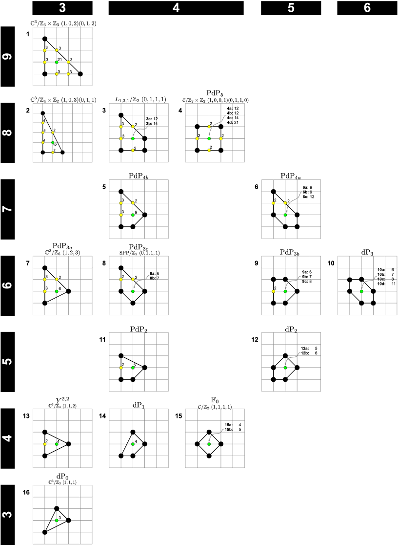
Figure 2.1: The 16 inequivalent reflexive polygons (up to SL$(2,\mathbb{Z})$). Figure taken from Hanany:2012hi (with slight modifications). The reflexive polygons are arranged such that the dual pairs are mirror symmetric with respect to the middle line (fourth row), and the four polygons in the middle line are therefore self-dual. In each row, the polygons have the same number of boundary points/(normalized) area. In each column, the polygons have the same number of vertices.

2.2.1 Tempered Polynomials

Given a Newton polygon, it is easy to construct the Newton polynomial, in reverse to what was discussed in the beginning of §2.2. Nevertheless, we still have the freedom to choose the complex coefficients in $P(z,w)$. In number theory and related study of Mahler measure, the so-called tempered families are of particular interest villegas1999modular ; boyd2002mahler .

Given a Newton polygon $\mathfrak{P}$, we obtain the Newton polynomial $P(z,w)=\sum c_{(m,n)}z^{m}w^{n}$ with coefficients $c_{(m,n)}$ for each of the lattice points. Now, consider a bounding edge $F$ of the polygon $\mathfrak{P}$. There might also be lattice points on it (the yellow points in Figure 2.1), in addition to the 2 endpoints (the black points in Figure 2.1) which are vertices of $\mathfrak{P}$. Suppose there are $N$ lattice points on $F$, indexed from 0 to $N-1$, and we call the associated coefficients $c_{(m,n)}$ as $c_{F,l}$. Then, we can create an auxiliary polynomial $P_{F}(t)\in\mathbb{C}[t]$ as

$$P_{F}(t)=\sum_{l=0}^{N-1}c_{F,l}t^{l}\ ,$$ (2.12)

for each edge $F$.

Notice that this automatically requires that the boundary point $c_{F_{1},N-1}$ to coincide with $c_{F_{2},0}$ for any two adjacent edges $F_{1}$ and $F_{2}$. A Laurent polynomial is then said to be tempered if the set of roots of $\prod\limits_{F\in\mathfrak{P}}P_{F}(t)$ consists of roots of unity only. In other words, each $P_{F}$ in $\mathfrak{P}$ would only have roots on the unit circle.

Notice that being tempered only gives restrictions to coefficients for the boundary points. For the reflexive polygons considered in this paper, we always take the single interior point as the origin, corresponding to the constant term $k$ in the Newton polynomial as discussed before: $P(z,w)=k-p(z,w)$.

Example 3.

For $\mathbb{F}_{0}$, $P=k-z-z^{-1}-w-w^{-1}$ is tempered. For instance, the lattice points $(1,0)$ and $(0,-1)$ corresponds to the monomials $-z$ and $-w^{-1}$ in $P$. The edge linking them is associated to the polynomial $-1-t$ which only has one root $t=-1$. In fact, every one of the 4 edges has the same polynomial $P_{F}=-1-t$. Thus, $P$ is tempered.

$t^{0}$	1	1	1	1	1	1	1	1	1	1	1	1	1	1	1	1	1	1	1	1	1	1	1	1	1
$t^{1}$	0	0	0	0	0	0	0	0	0	1	1	1	1	1	1	1	1	2	2	2	2	2	3	3	4
$t^{2}$	$-2$	$-2$	$-1$	0	0	0	1	1	2	$-1$	0	0	0	1	1	1	2	0	1	2	2	3	3	4	6
$t^{3}$	0	0	0	0	0	1	0	0	0	$-1$	$-1$	0	1	0	1	1	1	$-2$	0	1	2	2	1	3	4
$t^{4}$	1	0	1	$-1$	1	0	0	1	1	0	$-1$	0	1	0	0	1	1	$-1$	0	0	1	1	0	1	1

Table 2.1: Each column gives a set of coefficients for $P_{F}(t)$ such that the solutions to $P_{F}(t)=0$ only have roots of unity.

For reflexive polygons, all the possible $P_{F}$’s that make $P$ tempered have been classified in villegas1999modular . We reproduce it here in Table 2.1; there are 25 possibilities. For convenience, given a tempered Newton polynomial, if it only has non-zero coefficients for vertices, we shall call such choice minimally tempered coefficients. If all the boundary points have non-zero coefficients and the coefficients for every edge are binomial, that is, $P_{F}=(t+1)^{N}$ for all $F\in\mathfrak{P}$, then we shall call such choice maximally tempered coefficients. When a polygon has no boundary lattice points other than vertices (i.e., each edge has exactly the 2 endpoints which are lattice points), the minimally and maximally tempered coefficients coincide and this is the only set of tempered coefficients.

Example 4.

As we have seen, $\mathbb{F}_{0}$ has only one possible set of tempered coefficients. On the other hand, for $\mathbb{C}^{3}/(\mathbb{Z}_{4}\times\mathbb{Z}_{2})$ $(1,0,3)(0,1,1)$ (No.2 in Figure 2.1), there are $2\times 2\times 4=16$ tempered choices. When all the three faces have $P_{F}(t)=-t-1$, $P(z,w)$ is minimally tempered. If $P_{F_{1,2}}=-t^{2}-2t-1=-(t+1)^{2}$ and $P_{F_{3}}=-t^{4}-4t^{3}-6t^{2}-4t-1=-(t+1)^{6}$, then $P(z,w)$ is maximally tempered. Notice that the minus sign is just a convention here as it would not change the spectral curve $P=0$. All the maximally and minimally tempered Newton polynomials are listed in Appendix A.

Remark 1.

Returning to the Mahler measure, we checked the Mahler flow for the $16$ reflexive polygons from $k=0$ to tropical $k$ numerically. The Mahler measures are all strictly increasing when $k$ increases, which supports the Mahler flow conjecture in Bao:2021fjd .

2.2.2 Elliptic Curves

Since the reflexive polygons give elliptic curves, we here review some of the requisites from the geometry and number theory of elliptic curves. In general, any elliptic curve $E$ can be transformed into Weierstrass normal form

$$y^{2}=x^{3}+fx+g.$$ (2.13)

The curve is non-singular if and only if $\Delta\neq 0$, where

$$\Delta=-16(4f^{3}+27g^{2})$$ (2.14)

is known as the discriminant. Then the $j$-invariant is given by

$$j=\frac{4\times(24f)^{3}}{\Delta}.$$ (2.15)

This is a crucial concept since isomorphic (isogenous) elliptic curves have the same $j$-invariant. Notice that however $j$-invariant is only able to distinguish elliptic curves over algebraically closed fields.

Topologically, an elliptic curve $E$ is the torus $\mathbb{T}^{2}$. Hence, it is endowed with a complex structure specified by the two periods which are integrals along the two cycles $A$ and $B$ of the torus: $\int_{A,B}\frac{\text{d}x}{y}$. This complex structure should coincide with the $\tau$ computed from $u_{0,1}$ in (2.19) up to SL$(2,\mathbb{Z})$. As a function of $\tau$, $j(\tau):E\rightarrow\mathbb{P}^{1}$ is a modular function, i.e., invariant under SL$(2,\mathbb{Z})$ transformations. It is in fact the only modular function in that any meromorphic function which is SL$(2,\mathbb{Z})$-invariant is a rational function in $j(\tau)$.

Now, because our Newton polynomial (2.2) always has a parameter $k$, any reflexive polygon defines for us a family of elliptic curves. Geometrically, when $k\in\mathbb{C}\sqcup\infty$, this defines an elliptic fibration over $\mathbb{P}^{1}$, giving us a complex surface which is called a modular elliptic surface shioda1972elliptic ; He:2012jn . In this case, all the crucial quantities, such as $\Delta$ and $j$, depend on $k$. In particular, $j(k)$ can be seen as a map from $\mathbb{P}^{1}$ with coordinate $k$ to $\mathbb{P}^{1}$. We will make use of this map shortly.

2.3 Modular Mahler Measure

In general, the spectral curve $P(z,w)=0$ defines a Riemann surface as an algebraic curve $\Sigma$. Since each reflexive polygon has a single interior point, $\Sigma$ is genus one. For all but finitely many $k$’s, the curve would be a smooth elliptic curve. For convenience, let us define $\lambda:=k^{-1}$, then we have (where we explicitly write out the dependence of the elliptic curve on the parameter $\lambda$)

$$\Sigma_{\lambda}\ :\ 1-\lambda\ p(z,w)=0\ .$$ (2.16)

As pointed out in villegas1999modular , $u_{0}$ is a period of a holomorphic 1-form on $\Sigma_{\lambda}$. Hence, it satisfies the Picard-Fuchs equation

$$A(\lambda)\frac{\text{d}^{2}u_{0}}{\text{d}\lambda^{2}}+B(\lambda)\frac{\text{d}u_{0}}{\text{d}\lambda}+C(\lambda)u_{0}=0,$$ (2.17)

where $A(\lambda),B(\lambda),C(\lambda)$ are polynomials in $\lambda$. As we will see (in §3.3), this is actually a consequence of Theorem 3.8 kontsevich2001periods . We may then use the Picard-Fuchs equation to find the dual period $u_{1}$ of the form

$$u_{1}(\lambda)=u_{0}(\lambda)\log(\lambda)+v(\lambda),$$ (2.18)

where $v$ is a holomorphic function with $v(0)=0$. This defines

$$\tau=\frac{1}{2\pi i}\frac{u_{1}}{u_{0}},\quad q=\text{e}^{2\pi i\tau}=\lambda+\dots.$$ (2.19)

As usual, $\tau$ gives the complex structure of the elliptic curve $P=0$ as a torus. The monodromy around $\lambda=0$ (i.e., at $k$ infinity) acts as $\tau\rightarrow\tau+1$. This fixes $q$ and we may locally invert it to get

$$\lambda(\tau)=q+\dots,\quad u_{0}(\tau)=1+\dots.$$ (2.20)

Using the nome $q$, we can also express the Mahler flow equation (2.8) as

$$q\frac{\text{d}m}{\text{d}q}=\frac{\text{d}m}{\text{d}\lambda}\frac{q\text{d}\lambda}{\text{d}q}=\frac{u_{0}}{\lambda}\frac{q\text{d}\lambda}{\text{d}q}=:e(\tau).$$ (2.21)

In fact, $\lambda,u_{0},e$ are modular forms (with singularities) of weights 0, 1, 3 respectively under the monodromy of Picard-Fuchs equation, namely a congruence subgroup of SL$(2,\mathbb{Z})$ acting on $\tau$ villegas1999modular . We may therefore call (2.21) the modular Mahler flow equation.

Write the Fourier series of $e(\tau)$ as $e(\tau)=1+\sum\limits_{n=1}^{\infty}e_{n}q^{n}$. Then from (2.21), we have

Theorem 2.2 (Rodriguez-Villegas villegas1999modular ).

Locally around $\tau=i\infty$ (i.e., $\lambda=0$), we have

$$m(P)=-2\pi i\tau-\sum_{n=1}^{\infty}\frac{e_{n}}{n}q^{n}.$$ (2.22)

Because of the modularity of $e(\tau)$, the Mahler measure for elliptic curves is referred to as modular Mahler measure though $m(P)$ itself is not modular.

Example 5.

For $P(z,w)=\lambda^{-1}-z-z^{-1}-w-w^{-1}$, $m(P)$ and $u_{0}$ are given in (2.9). Since $u_{0}$ is hypergeometric, it is easy to see that the Picard-Fuchs equation is

$$\mu(16\mu-1)\frac{\textup{d}^{2}u}{\textup{d}\mu^{2}}+(32\mu-1)\frac{\textup{d}u}{\textup{d}\mu}+4u=0,$$ (2.23)

where we have used $\mu:=\lambda^{2}$ for convenience. This leads to villegas1999modular

$$u_{1}=u_{0}\log(\mu)+8\mu+84\mu^{2}+\frac{2960}{3}\mu^{3}+\dots,$$ (2.24)

and

$$u_{0}=1+4\sum_{n=1}^{\infty}\sum_{d|n}\chi_{-4}(d)q^{n},\quad e=1-4\sum_{n=1}^{\infty}\sum_{d|n}\chi_{-4}(d)d^{2}\,q^{n},\quad\mu=\frac{1}{c^{2}}\left(\sum_{\begin{subarray}{c}n=1\\ n\textup{ odd}\end{subarray}}^{\infty}\sum_{d|n}d\,q^{n}\right),$$ (2.25)

where $\chi_{-4}$ is the Dirichlet character/Kronecker symbol satisfying $\chi_{-4}(n)=1,0$ when $n\equiv 0,1~{}(\textup{mod }2)$. Then, we have

$$m(P)=\frac{16\,\textup{Im}\tau}{\pi^{2}}\sum_{\begin{subarray}{c}n_{1},n_{2}\in\mathbb{Z}\\ (n_{1},n_{2})\neq(0,0)\end{subarray}}\frac{\chi_{-4}(n_{1})}{(n_{1}+4n_{2}\tau)^{2}(n_{1}+4n_{2}\bar{\tau})},$$ (2.26)

which under modular transformations, we have

$$\begin{split}&\tau\rightarrow-\frac{1}{\tau}:\quad m=\frac{16\,\textup{Im}\bar{\tau}}{\pi^{2}}\sum_{\begin{subarray}{c}n_{1},n_{2}\in\mathbb{Z}\\ (n_{1},n_{2})\neq(0,0)\end{subarray}}\frac{\chi_{-4}(n_{1})\tau}{(4n_{2}-n_{1}\tau)^{2}(4n_{2}-n_{1}\bar{\tau})},\\ &\tau\rightarrow\tau+1:\quad m=\frac{16\,\textup{Im}\tau}{\pi^{2}}\sum_{\begin{subarray}{c}n_{1},n_{2}\in\mathbb{Z}\\ (n_{1},n_{2})\neq(0,0)\end{subarray}}\frac{\chi_{-4}(n_{1})}{(n_{1}+4n_{2}\tau)^{2}(n_{1}+4n_{2}\bar{\tau})}.\end{split}$$ (2.27)

Hence, $m$ is invariant under monodromy ($\tau\rightarrow\tau+1$) at $k\rightarrow\infty$ while we have $m\rightarrow 0$ as $\tau\rightarrow 0$. We expect this to be true in general for reflexive polygons.

2.4 Esquisse de Dessins, or Sketches of Children’s Drawings

The discussions on elliptic curves above are initmately related to the profound theorem by Belyi belyui1980galois :

Theorem 2.3.

Let $\mathcal{X}$ be a compact, connected Riemann surface. Then $\mathcal{X}$ is a non-singular, irreducible projective variety of complex dimension $1$ and can be defined by polynomial equations. The defining polynomial has algebraic coefficients if and only if there exists a rational map $\beta:\mathcal{X}\rightarrow\mathbb{P}^{1}$ which is ramified at exactly three points, that is, has three critical values.

We will be primarily concerned with the case of $\mathcal{X}=\mathbb{P}^{1}$, so that the Belyi map is a rational function $p(x)/q(x):\mathbb{P}^{1}\rightarrow\mathbb{P}^{1}$. Now, on the target $\mathbb{P}^{1}$, any three points can be taken to be 0, 1 and $\infty$ (that is, $[0:1]$, $[1:1]$ and $[1:0]$ in homogenous coordinates) by linear-fractional Möbius transformations, so that the three ramified points can be thus chosen. Following Grothendieck Grothendieck1984sketch , a bipartite graph called dessin d’enfant (or child’s drawing) can be associated to $\beta$ by

$$\begin{split}&B=\beta^{-1}(0)=\{x\in\mathbb{P}^{1}~{}|~{}p(x)=0\},\quad W=\beta^{-1}(1)=\{x\in\mathbb{P}^{1}~{}|~{}p(x)=q(x)\},\\ &E=\beta^{-1}([0,1])=\{x\in\mathbb{P}^{1}~{}|~{}p(x)=tq(x),\text{ for some $t\in[0,1]$}\},\\ &F=\beta^{-1}(\infty)=\{x\in\mathbb{P}^{1}~{}|~{}q(x)=0\},\end{split}$$ (2.28)

where $B$, $W$, $E$ and $F$ denote the black, white vertices, edges and faces respectively. As $\beta$ is $\mathbb{P}^{1}\rightarrow\mathbb{P}^{1}$, the graph is embedded on a sphere. Moreover,

Proposition 2.4.

Let $\beta:\mathbb{P}^{1}\rightarrow\mathbb{P}^{1}$ be a Belyi map. Then the associated bipartite graph $(V=B\sqcup W,E,F)$ is loopless, connected and planar. It has $|V|=|\beta^{-1}(\{0,1\})|$ vertices, $|E|=\deg(\beta)$ edges and $|F|=|\beta^{-1}(\infty)|$ faces, satisfying $|V|-|E|+|F|=2$.

As we will plot the dessin on a plane via stereographic projection, all the bounded faces on the plane are called internal faces while the face containing $k\rightarrow\infty$ is known as the external face. As $\beta$ is a multi-covering of the target $\mathbb{P}^{1}$, we can consider the monodromy around each vertex in the dessin. Essentially, each monodromy acting on a vertex permutes the edges connected to that vertex. We shall denote the set of such permutations around black (white) vertices as $\sigma_{0}$ ($\sigma_{1}$). Then $\sigma_{0}$ and $\sigma_{1}$ generate a free group known as the monodromy/cartographic group $G$ of the dessin. In particular, the monodromies $\sigma_{\infty}$ around faces can be obtained by $\sigma_{\infty}\circ\sigma_{1}\circ\sigma_{0}=1$. As the dessin has $|E|$ edges, $G$ is a subgroup of the symmetric group $\mathfrak{S}_{N}$ where $N=|E|!$.

In our context, recall that all our elliptic curves $E$ are parametrized by $k$ so that the Klein invariant $j(k)$ is a function of the parameter $k$ and is thus a map from $\mathbb{P}^{1}$ (instead of $E$) to $\mathbb{P}^{1}$. We will show in §3.1 that $j(k)$ is actually Belyi for maximally tempered coefficients in the Newton polynomials:

$$\beta=\frac{j}{1728}\ .$$ (2.29)

Congruence subgroups and coset graphs

A coset graph is a graph associated with a group $K$ generated by elements $\{x_{i}\}$ and a subgroup $H$. Then each vertex (drawn in black so as to reconstruct the dessin) in the coset graph represents a right coset $Hg$ for $g\in K$. An edge is of form $(Hg,Hgx_{i})$ which connects the coset $Hg$ and $H(gx_{i})$.

As we will see shortly, the dessins associated to reflexive polygons (with maximally tempered coefficients) are clean, namely that the white vertices all have valency $2$. Therefore, the dessins can be viewed as coset graphs by removing the white vertices. Conversely, we can insert a white vertex on each edge to get the dessin from the coset graph.

In particular, the dessins we will consider in §3 are associated with the modular group (P)SL$(2,\mathbb{Z})$ and the congruence subgroups. Hence, the generators can be taken as the usual $S$ and $T$, viz,

$$S=\begin{pmatrix}0&-1\\ 1&0\end{pmatrix},\quad T=\begin{pmatrix}1&1\\ 0&1\end{pmatrix}\quad\text{s.t. PSL}(2,\mathbb{Z})=\langle S,T|S^{2}=(ST)^{3}=1\rangle.$$ (2.30)

The congruence groups of level $n$ are defined as

$$\begin{split}&\Gamma(n):=\left\{M\in\text{(P)SL}(2,\mathbb{Z})\Bigg{|}M\equiv\begin{pmatrix}1&0\\ 0&1\end{pmatrix}~{}(\text{mod }n)\right\},\\ &\Gamma_{1}(n):=\left\{M\in\text{(P)SL}(2,\mathbb{Z})\Bigg{|}M\equiv\begin{pmatrix}1&b\\ 0&1\end{pmatrix}~{}(\text{mod }n)\right\},\\ &\Gamma_{0}(n):=\left\{M\in\text{(P)SL}(2,\mathbb{Z})\Bigg{|}M\equiv\begin{pmatrix}a&b\\ 0&d\end{pmatrix}~{}(\text{mod }n)\right\}.\end{split}$$ (2.31)

In particular, we have $\Gamma(n)\leq\Gamma_{1}(n)\leq\Gamma_{0}(n)$ and $\Gamma_{0}(n_{2})\leq\Gamma_{0}(n_{1})$ if $n_{1}|n_{2}$. The fact that every congruence subgroup of (P)SL$(2,\mathbb{Z})$ has a coset graph (called Schreier-Cayley graph) which is a clean trivalent dessin was discussed in He:2012kw ; He:2012jn ; Tatitscheff:2018aht .

Given a congruence subgroup $\Gamma$, the quotient space $\mathfrak{h}/\Gamma$ (where $\mathfrak{h}$ is the upper half plane) can be compactified by adding a few isolated points (aka cusps of $\Gamma$). Such compactified curve $X(\Gamma)$ is called the modular curve. The genus of $\Gamma$ is then defined to be the genus of $X(\Gamma)$. When $X(\Gamma)$ is of genus 0, the field of meromorphic functions on $X(\Gamma)$ is generated by a single element known as a Hauptmodul of $\Gamma$.

2.5 Dimers and Quivers

Having introduced the requisite mathematical concepts, let us now proceed to some physics. With so-called forward and inverse algorithms, one can construct a Newton polygon, which encodes a toric CY 3-fold, from a brane tiling, which encodes a quiver gauge theory in (3+1)-dimensions with $\mathcal{N}=1$ supersymmetry, and vice versa. From a tiling, we may then get a toric quiver as its dual graph which encodes certain supersymmetric gauge theories. Here, we will not explain the details and the readers are referred to Feng:2000mi ; Hanany:2005ve ; Franco:2005rj ; Franco:2005sm ; Feng:2005gw . Instead, we will only introduce the necessary concepts for this paper.

A perfect matching of a bipartite graph is a collection of edges such that each vertex is incident to exactly one edge. The bipartite nature then means that each edge connects one white with one black node. The dimer model is then the study of (random) perfect matchings Kenyon:2003uj ; kenyon2003introduction . Physically, the dimer models are also called brane tilings as they have a nice interpretation in terms of brane systems. In particular, the dimers discussed here are all $\mathbb{Z}^{2}$-periodic and embedded in $\mathbb{T}^{2}$.

Given a perfect matching $M$, there is a unit flow $\omega$ along each edge in $M$ from a white to a black node. Consider a reference perfect matching $M_{0}$ with flow $\omega_{0}$ and a path from face $f_{0}$ to $f_{1}$ in the graph. Then for any $M$ with flow $\omega$, the total flux of $\omega-\omega_{0}$ across the path defines a path-independent height function of $M$. The difference of height functions of any two perfect matchings is independent of the choice of $M_{0}$. The height change is then $(h_{x},h_{y})$ if the horizontal and vertical height changes of $M$ (for one period) are $h_{x}$ and $h_{y}$ respectively.

Moreover, we can assign some (real) energy function to each edge $e$. Then given a perfect matching $M$, its energy is $\mathcal{E}(M):=\sum\limits_{e\in M}\mathcal{E}(e)$. For any edge $e$ in the graph, its edge weight is defined to be $\textup{e}^{-\mathcal{E}(e)}$.

With all these quantities, we can then obtain the associated Newton polynomial as Kenyon:2003uj

$$P(z,w)=\sum_{M}\text{e}^{-\mathcal{E}(M)}z^{h_{x}}w^{h_{y}}(-1)^{h_{x}h_{y}+h_{x}+h_{y}}.$$ (2.32)

Moreover, from this expression, we can see that each perfect matching $M$ is associated to a lattice point $(h_{x},h_{y})$ in the Newton polygon. Hence, we shall call a perfect matching external (internal) if it corresponds to an external (internal) point in the toric diagram. Physically, the perfect matchings are in one-to-one correspondence with gauged linear sigma model fields. The perfect matchings associated to each point are explicitly labelled in Figure 2.1 for reflexive polygons. Since the polygon/tiling correspondence is one-to-many, the different numbers assigned to the interior point of a polygon are from different tilings/toric phases. Notice that each vertex corresponds to exactly one perfect matching.

Canonical edge weights

There is a special choice of edge weights which comes from the R-charges of the fields in the quiver theory. Since the quiver is the dual diagram, each arrow corresponds to an edge in the tiling. As each arrow is physically a multiplet, we can relate its R-charge $R$ to the corresponding edge in the tiling as follows. As an edge always belongs to two faces, we can connect the centre points of the faces and the two endpoints of the edge to form a rhombus. Then the rhombus angle $\theta$ satisfies $2\theta=\pi R$, where $2\theta$ is the angle of the rhombus at the vertex that has in common with the edge.

In particular, the edge would then have length $2\cos(\theta)$. This is often the situation for isoradial dimers whose faces can all be inscribed in a circle of the same radius. Nevertheless, as discussed in Bao:2021fjd , this R-charge/rhombus angle setting could also be extended to non-isoradial dimers if one thinks of zero or negative edge lengths. Then the canonical weight of an edge is $2\sin(\pi R/2)$. With such canonical weights, one can find many interesting features of quiver gauge theories regarding the Newton polynomials and Mahler measures. See Bao:2021fjd for more details.

Example 6.

Let us consider the tiling in Figure 2.2(a).

(a)

(b)

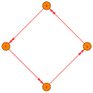
(c)

Figure 2.2: (a) The dimer model. (b) The toric diagram. (c) The quiver diagram.

The canonical weight for an edge is always $\sqrt{2}$. Using (2.32), one can find that the curve is given by

$$-2z-2z^{-1}-2w-2w^{-1}+(2+2+2+2)=0,$$ (2.33)

or, equivalently,

$$-z-z^{-1}-w-w^{-1}+4=0.$$ (2.34)

We see that the corresponding Newton polygon is our running reflexive example, shown in 2.2(b). The quiver in Figure 2.2(c) is the dual graph of the dimer. This is the well-known phase I (corresponding to No.15 (a) in Figure 2.1) of the D-brane worldvolume quiver gauge theory for the CY 3-fold which is the cone over the Fano toric surface $\mathbb{F}_{0}=\mathbb{P}^{1}\times\mathbb{P}^{1}$. In this example, we find that Newton polynomial obtained from canonical weights coincide with the one with (maximally) tempered coefficients (at $k=4$).

In general, coefficients from canonical weights are not necessarily the same as maximally tempered coefficients.

Specular duality

As studied in Hanany:2012vc , the quiver gauge theories enjoy specular duality under which the master spaces are preserved. In short, the master space $\mathcal{F}^{\flat}$ Forcella:2008eh ; Forcella:2008bb is the space of solutions to the F-term relations (more strictly, the maximal spectrum of the coordinate ring quotiented by the ideal of F-terms). Its largest irreducible component is known as the coherent component ${}^{\text{Irr}}\mathcal{F}^{\flat}$, which can be written as a symplectic quotient in terms of perfect matchings $M_{i}$:

$${}^{\text{Irr}}\mathcal{F}^{\flat}=\mathbb{C}[M_{i}]//Q_{F},$$ (2.35)

where $Q_{F}$ is the F-term charge matrix Feng:2000mi .

Remark 2.

It was shown in Bao:2021fjd that $u_{0}(k)$ is the generating function of the master space in terms of F-term charge matrix though the F-term relations in higher orders are just redundant. Following Bao:2021fjd , $k\rightarrow\infty$ is known as a tropical limit when $P(z,w)=k-p(z,w)$. As a result, this is equivalent to $q\rightarrow 0$ and hence $\tau\rightarrow i\infty$. Physically, $\tau$ can be interpreted as the complexified gauge coupling in type IIB string theory, that is, $\tau=\frac{\theta}{2\pi}+\frac{i}{g_{\textup{IIB}}}$. Therefore, this gives the weak coupling $g_{\textup{IIB}}\rightarrow 0$. For the modular forms (with singularties) introduced before, we have $\lambda\rightarrow 0$, $u_{0}\rightarrow 1$ and $e\rightarrow 1$. In particular, $u_{0}\rightarrow 1$ indicates a free theory in the tropical limit as the master space become trivial. This is consistent with the weakly coupled gauge theory with $\tau\rightarrow i\infty$.

Moreover, we have $m$ tends to $\infty$ for tropical $k$. On the other hand, $m$ would go to $0$ in the strong coupling regime (as $\tau\rightarrow 0$).

For reflexive polygons, the specular duals are Hanany:2012vc

$$1\leftrightarrow 1~{},~{}$$

$$2\leftrightarrow 4d~{},~{}3a\leftrightarrow 4c~{},~{}3b\leftrightarrow 3b~{},~{}4a\leftrightarrow 4a~{},~{}4b\leftrightarrow 4b~{},~{}$$

$${\color[rgb]{1,0,0}5}\leftrightarrow{\color[rgb]{1,0,0}6}c~{},~{}6a\leftrightarrow 6a~{},~{}6b\leftrightarrow 6b~{},~{}$$

$$7\leftrightarrow 10d~{},~{}8a\leftrightarrow 10c~{},~{}8b\leftrightarrow{\color[rgb]{1,0,0}9}c~{},~{}{\color[rgb]{1,0,0}9}a\leftrightarrow 10b~{},~{}9b\leftrightarrow 9b~{},~{}10a\leftrightarrow 10a~{},~{}$$ (2.36)

$${\color[rgb]{1,0,0}11}\leftrightarrow 12b~{},~{}12a\leftrightarrow 12a~{},~{}$$

$$13\leftrightarrow 15b~{},~{}14\leftrightarrow 14~{},~{}15a\leftrightarrow 15a~{},~{}$$

$$16\leftrightarrow 16~{},$$

where the letters following the number label different toric phases as in Figure 2.1. As we can see, their internal and external perfect matchings get exchanged under specular duality.

Remark 3.

The red numbers in the above list contain polygons that are called exceptional cases due to the following two reasons Bao:2021fjd .

• With canonical weights, most of the specular duals can have the same Mahler measure (with the constant term taken to be $k$) up to an additive constant, that is, $m(P_{2})=m(P_{1})+\kappa$. Hence, by an overall scaling of factor $\textup{e}^{-\kappa}$, we have $k-p_{1}\rightarrow k-\textup{e}^{-\kappa}p_{1}$ (notice that this does not change the spectral curve $P_{1}=0$). Thus, $m(P_{2})=m(P_{1})$. As a result, for example, polygons No.2 and No.3 have the same Mahler measure as they are connected by different toric phases of No.4 even though they are not specular duals. However, it turns out that No.5, 6, 9 and 11 do not satisfy this property.

• Moreover, with canonical weights (with constant term $k$), most Newton polynomials can have equal coefficients for vertices under rescaling of $z$ and/or $w$. However, this is not possible for No.5, 6, 9 and 11.

It is worth noting that the exceptions of the above two properties coincide (though the reason why they coincide is still unclear). It is still not known why No.5, 6, 9, 11 are exceptional. In §3.1, we will see that they are further exceptional regarding a third property.

Example 7.

The toric phase (b) for No.15 is specular dual to the single toric phase for No.13. Indeed, No.15(b) has $4$ external and $5$ internal perfect matchings while No.13 has $5$ external and $4$ internal perfect matchings. A more detailed analysis on the two theories under specular duality can be found in Hanany:2012vc .

3 Modularity and Gauge Theories

Having introduced all the background, we are now ready to discuss how modular Mahler measures connected the various different areas in mathematics and physics. From §2, the readers may have already noticed that

Proposition 3.1.

The maximally tempered coefficients in the Newton polynomials are equal to the numbers of perfect matchings associated to the exterior lattice points of the toric diagrams.

Hence, we will mainly focus on maximally tempered coefficients in the following discussions, and we will see various properties implying potential physical relevance. As listed in Bao:2020kji , all the non-reflexive polygons with two interior points also have maximally tempered coefficients equal to the numbers of perfect matchings associated to the boundary points (it would also be interesting to see what happens for higher dimensional reflexive polytopes He:2017gam ). Furthermore, the consistent brane tilings for all polygons presented in Davey:2009bp also have maximally tempered coefficients while the remaining inconsistent tilings do not. Therefore, it is natural to conjecture that

Conjecture 3.2.

A brane tiling is consistent if and only if the corresponding toric diagram (either reflexive or non-reflexive) has maximally tempered coefficients for its boundary points. Moreover, the maximally tempered coefficients are equal to the numbers of perfect matchings associated to the boundary points.

It is curious that maximal tempered coefficients appear in two completely different contexts, one from perfect matching in physics and another from considering Mahler measure in mathematics.

3.1 Dessins and Mahler Measure

As mentioned throughout, we will focus on the 16 reflexive polygons with maximally tempered coefficients. The Newton polynomials are listed in Table LABEL:Pzwmaxmin. Recall that the spectral curve $P(z,w)=0$ for each reflexive polygon is an elliptic curve (except for finitely many $k$ values). We can transform the spectral curves into Weierstrass normal form $y^{2}=x^{3}+f(k)x+g(k)$ (recall that all our elliptic curves depend on the parameter $k$). This is computationally rather involved (Nagell’s algorithm) but can luckily be done with SAGE sage .

In Table LABEL:refelliptic, we list the Weierstrass form of all 16 reflexive polygons with maximally tempered coefficients, where the coefficients $f(k)$ and $g(k)$ all assume the form

$$f=-\frac{1}{48}k^{4}+a(k),\quad g=\frac{1}{864}k^{6}+b(k).$$ (3.1)

Table 3.1: The data of the elliptic curves for reflexive polygons with maximally tempered coefficients. We also list the values of $k$ when the spectral curve becomes singular for each case. Here, $\kappa_{1,2,3}$ are the three roots to $k^{3}+k^{2}-18k-43=0$ ($\kappa_{1}\approx 4.73$, $\kappa_{2,3}\approx-2.86\pm 0.94\text{i}$) while $\kappa_{5,6,7,8}$ are the four roots to $k^{4}+k^{3}-8k^{2}-36-11=0$ ($\kappa_{5}\approx-0.33$, $\kappa_{6}\approx 3.80$, $\kappa_{7,8}\approx-2.23\pm 1.94\text{i}$).

Polygon(s)	No.1	No.2, 3, 4
$a(k)$	$\frac{9}{2}k^{2}+36k+81$	$\frac{5}{3}k^{2}+8k+\frac{32}{3}$
$b(k)$	$-\frac{3}{8}k^{4}-4k^{3}-\frac{27}{2}k^{2}+54$	$-\frac{5}{36}k^{4}-\frac{2}{3}k^{3}+\frac{8}{9}k^{2}+\frac{32}{3}k+\frac{448}{27}$
Singular $k$	$-6$, $21$	$-4$, $12$
Polygon(s)	No.5, 6	No.7, 8, 9, 10
$a(k)$	$\frac{5}{6}k^{2}+\frac{5}{2}k+\frac{5}{3}$	$\frac{1}{2}k^{2}+k$
$b(k)$	$-\frac{5}{27}k^{4}-\frac{5}{24}k^{3}+\frac{5}{9}k^{2}+\frac{19}{6}k+\frac{395}{108}$	$-\frac{1}{24}k^{4}-\frac{1}{12}k^{3}+\frac{1}{4}k^{2}+k+1$
Singular $k$	$-3$, $\frac{5}{2}(1\pm\sqrt{5})$	$-3$, $-2$, $6$
Polygon(s)	No.11, 12	No.13, 15
$a(k)$	$\frac{1}{3}k^{2}+\frac{1}{2}k-\frac{1}{3}$	$\frac{1}{3}k^{2}-\frac{1}{3}$
$b(k)$	$-\frac{1}{36}k^{4}-\frac{1}{24}k^{3}+\frac{5}{36}k^{2}+\frac{1}{3}k+\frac{35}{108}$	$-\frac{1}{36}k^{4}+\frac{5}{36}k^{2}+\frac{2}{27}$
Singular $k$	$-1$, $\kappa_{1,2,3}$	$0$, $\pm 4$
Polygon(s)	No.14	No.16
$a(k)$	$\frac{1}{6}k^{2}+\frac{1}{2}k-\frac{1}{3}$	$\frac{1}{2}k$
$b(k)$	$-\frac{1}{72}k^{4}-\frac{1}{24}k^{3}+\frac{1}{18}k^{2}+\frac{1}{6}k+\frac{19}{108}$	$-\frac{1}{24}k^{3}+\frac{1}{4}$
Singular $k$	$\kappa_{5,6,7,8}$	$-3$, $\frac{3}{2}(-1\pm\text{i}\sqrt{3})$

We find that specular duals have exactly the same elliptic curve. Notice that this property only holds for maximally tempered coefficients. Recall that the maximally tempered coefficients indicate the number of perfect matchings for each lattice point and that specular duality exchange internal and external perfect matchings. Again, we see that maximally tempered coefficients are of particular physical interest.

We also tabulate all the values of $k$ that make each spectral curve $P=0$ singular in Table LABEL:refelliptic. They can be obtained by checking whether the discriminant of the curve vanishes. It is worth mentioning that in many cases, there exists a singular $k$ such that $|k|$ is equal to the minimal number of internal perfect matchings for the polygon. For instance, No.4 has four toric phases, the numbers of internal perfect matchings are 12, 12, 14 and 21 respectively. Indeed, there is a singular $k=|k|=12$. However, five of the reflexive polygons do not obey this observation: No. 5, 6, 11, 14 and 12. We find that the first four polygons coincide with the exceptional cases in Remark 3 while No.12 is the specular dual of (the exceptional) No.11.

Dessins d’Enfants

Given the elliptic curves in Table LABEL:refelliptic, we can then compute their $j$-invariants as in Table 3.2.

Polygon(s)	No.1	No.2, 3, 4	No.5, 6	No.7, 8, 9, 10
$j(k)$	$\frac{(k-18)^{3}(k+6)}{k-21}$	$\frac{(k^{2}-8k-32)^{3}}{k^{2}-8k-48}$	$\frac{(k^{4}-40k^{2}-120k-80)^{3}}{(k+3)^{5}(k^{2}-5k-25)}$	$\frac{k^{3}(k^{3}-24k-48)^{3}}{(k-6)(k+2)^{3}(k+3)^{2}}$
Polygon(s)	No.11, 12	No.13, 15	No.14	No.16
$j(k)$	$\frac{(k^{4}-16k^{2}-24k+16)^{3}}{(k+1)^{2}(k^{3}+k^{2}-18k-43)}$	$\frac{(k^{4}-16k^{2}+16)^{3}}{k^{2}(k^{2}-16)}$	$\frac{(k^{4}-8k^{2}-24k+16)^{3}}{k^{4}+k^{3}-8k^{2}-36k-11}$	$\frac{k^{3}(k^{3}-24)^{3}}{k^{3}-27}$

Table 3.2: The $j$-invariants for the elliptic curves.

Notice that in terms of the $k$ parameter, this is a map $j:\mathbb{P}^{1}\rightarrow\mathbb{P}^{1},k\mapsto j(k)$. In particular, the preimage $\mathbb{P}^{1}\cong S^{2}$ is the space of $k$, and hence parametrizes the Mahler flow. We will discuss this in more details in §3.4. By further checking $j(k)/1728$, we find that all of them are Belyi. Therefore, we can plot the corresponding dessins as in Figure 3.1 based on the Mathematica package from Goins .

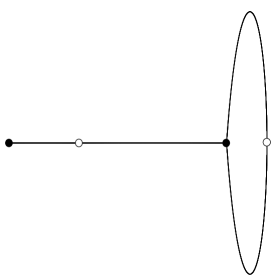
(a) No.1: $\{1^{1}3^{1},2^{2},1^{1}3^{1}\}$, $\Gamma_{0}(3)$

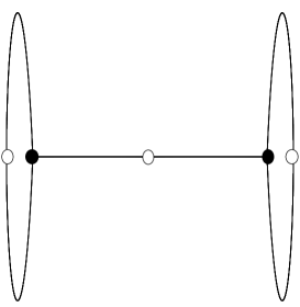
(b) No.2, 3, 4: $\{3^{2},2^{3},1^{2}4^{1}\}$, $\Gamma_{0}(4)$

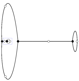
(c) No.5, 6: $\{3^{4},2^{6},1^{2}5^{2}\}$, $\Gamma_{1}(5)$

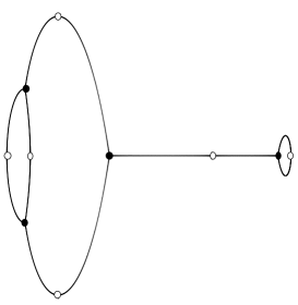
(d) No.7, 8, 9, 10: $\{3^{4},2^{6},1^{1}2^{1}3^{1}6^{1}\}$, $\Gamma_{0}(6)$

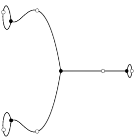
(e) No.11, 12: $\{3^{4},2^{6},1^{3}9^{1}\}$, $\Gamma_{0}(9)$

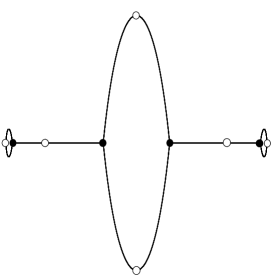
(f) No.13, 15: $\{3^{4},2^{6},1^{2}2^{1}8^{1}\}$, $\Gamma_{0}(8)$

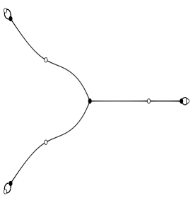
(g) No.14: $\{3^{4},2^{6},1^{3}9^{1}\}$, $\Gamma_{0}(9)$

(h) No.16: $\{3^{4},2^{6},1^{3}9^{1}\}$, $\Gamma_{0}(9)$

Figure 3.1: The dessins for reflexive polygons with maximally tempered coefficients, their passports and the corresponding congruence subgroups.

Here, the plots for the dessins are rigid in the sense that the vertices and edges are at the precise positions of $k=j^{-1}$ on $S^{2}\cong\mathbb{C}\sqcup\{\infty\}$ (except the part in the dashed blue box in (c) where we have to zoom in since the vertices $j^{-1}(0)$ and $j^{-1}(1)$ are too close to each other). As a result, the dessins in (e, g, h) have different “shapes” though they are isomorphic graphs.

As we have checked the reflexive polygons case by case, we conclude that

Proposition 3.3.

With maximally tempered coefficients for all 16 reflexive polygons, the family of elliptic curves, depending on $k$, are modular elliptic surfaces such that the $j$-invariants $j(k)$ are Belyi maps. Furthermore, specular dual reflexive polygons, regardless of which toric phases, give rise to the same elliptic curve, and hence the same $j$-invariant and dessin.

Remark 4.

Different toric phases for a reflexive polygon are often not related by specular duality, but they would still lead to the same elliptic curve/dessin as these phases would only differ by the multiplicity of the interior point. Since the master space is invariant under specular duality, this hints that the corresponding elliptic curve and dessin should encode some common features of the master spaces in different phases.

Remark 5.

In fact, $j(k)/1728$ being Belyi is generally true only for maximally tempered coefficients. For any other coefficient choices which are not physical in the sense of counting perfect matchings, the maps may or may not be Belyi. See Appendix B for example.

Although specular duals have the same elliptic curve, this does not directly imply that they should have the same Mahler measure as the Weierstrass normal form is obtained from the spectral curve under some bi-rational transformation while Mahler measure is only GL$(2,\mathbb{Z})$ invariant. Of course, we can compute the Mahler measures for reflexive polygons and likewise check case by case to show that specular duals have the same Mahler measure. Nevertheless, there is a more general proof using the Corollary 3.14.1 in Bao:2021fjd :

Lemma 3.4.

Given a pair of specular duals $a$ and $b$, suppose that the perfect matchings are mapped under $M_{i}^{a}\leftrightarrow M_{i}^{b}$. If their Newton polynomials are $P_{a,b}(z,w)=k-p_{a,b}(z,w)$, then for $|k|\geq\max\limits_{|z|=|w|=1}(|p_{a}|,|p_{b}|)$, the two Mahler measures have the series expansions

$$m(P_{a,b})=\log(k)-\sum_{n=2}^{\infty}\frac{f_{n}(M_{i}^{a,b})}{nk^{n}},$$ (3.2)

where $f_{n}$ are functions of $M_{i}^{a,b}$, and we have simply used $M_{i}^{a,b}$ to denote the weight for the corresponding perfect matching.

Now we can “unrefine” this by taking $M_{i}^{a,b}=1$. Then, we get the maximally tempered coefficients since they give the numbers of corresponding perfect matchings for the lattice points. Therefore,

Proposition 3.5.

With maximally tempered coefficients, the Mahler measure is invariant under specular duality.

In particular,

Corollary 3.5.1.

The reflexive polygons with maximally tempered coefficients have the same Mahler measure under specular duality.

Remark 6.

As Proposition 3.5 is a general statement, if two non-reflexive polygons have specular dual phases, then they would also have the same Mahler measure. Notice however the maximally tempered coefficients would now also fix all the coefficients for the interior points to be the corresponding numbers of perfect matchings except the origin with coefficient $k$.

Remark 7.

As Mahler measure is $\textup{GL}(2,\mathbb{Z})$ invariant, equivalent lattice polygons which are classified up to $\textup{SL}(2,\mathbb{Z})$ transformations would have the same Mahler measure.

For reference, we list the Mahler measures for reflexive polygons with maximally tempered coefficients in Table LABEL:refmahler.

Table 3.3: The Mahler measure up to order 10 for reflexive polygons with maximally tempered coefficients. Here, we restrict $k\geq\max\limits_{|z|=|w|=1}\{|p(z,w)|\}$. If $|k|\geq\max\limits_{|z|=|w|=1}\{|p(z,w)|\}$ (i.e., not necessarily real), then $\mathtt{m}(P)$ is just the real part of these expressions.

No.1	$\log(k)-\frac{27}{k^{2}}-\frac{164}{k^{3}}-\frac{4941}{2k^{4}}-\frac{31752}{k^{5}}-\frac{479940}{k^{6}}-\frac{7426080}{k^{7}}$
	$-\frac{482173965}{4k^{8}}-\frac{6030521840}{3k^{9}}-\frac{171779570802}{5k^{10}}-\dots$
No.2, 3, 4	$\log(k)-\frac{10}{k^{2}}-\frac{32}{k^{3}}-\frac{297}{k^{4}}-\frac{2112}{k^{5}}-\frac{55720}{3k^{6}}-\frac{163200}{k^{7}}$
	$-\frac{3038665}{2k^{8}}-\frac{43406720}{3k^{9}}-\frac{141433992}{k^{10}}-\dots$
No.5, 6	$\log(k)-\frac{5}{k^{2}}-\frac{10}{k^{3}}-\frac{135}{2k^{4}}-\frac{312}{k^{5}}-\frac{5675}{3k^{6}}-\frac{11100}{k^{7}}$
	$-\frac{280175}{4k^{8}}-\frac{1346800}{3k^{9}}-\frac{2962386}{k^{10}}-\dots$
No.7, 8, 9, 10	$\log(k)-\frac{3}{k^{2}}-\frac{4}{k^{3}}-\frac{45}{2k^{4}}-\frac{72}{k^{5}}-\frac{340}{k^{6}}-\frac{1440}{k^{7}}$
	$-\frac{27405}{4k^{8}}-\frac{96880}{3k^{9}}-\frac{794178}{5k^{10}}-\dots$
No.11, 12	$\log(k)-\frac{2}{k^{2}}-\frac{2}{k^{3}}-\frac{9}{k^{4}}-\frac{24}{k^{5}}-\frac{245}{3k^{6}}-\frac{200}{k^{7}}$
	$-\frac{2065}{2k^{8}}-\frac{12320}{3k^{9}}-\frac{75852}{5k^{10}}-\dots$
No.13, 15	$\log(k)-\frac{2}{k^{2}}-\frac{9}{k^{4}}-\frac{200}{3k^{6}}-\frac{1225}{2k^{8}}-\frac{31752}{5k^{10}}-\dots$
	$=\log k-2k^{-2}{}_{4}F_{3}\left(1,1,\frac{3}{2},\frac{3}{2};2,2,2;16k^{-2}\right)$
No.14	$\log(k)-\frac{1}{k^{2}}-\frac{2}{k^{3}}-\frac{3}{2k^{4}}-\frac{12}{k^{5}}-\frac{55}{3k^{6}}-\frac{60}{k^{7}}$
	$-\frac{875}{4k^{8}}-\frac{1400}{3k^{9}}-\frac{9576}{5k^{10}}-\dots$
No.16	$\log(k)-\frac{2}{k^{3}}-\frac{15}{k^{6}}-\frac{560}{3k^{9}}-\dots$
	$=\log(k)-6k^{-3}{}_{4}F_{3}\left(1,1,\frac{4}{3},\frac{5}{3};2,2,2;27k^{-3}\right)$

It is then also straightforward to get the expression for $u_{0}(k)$, which reads

$$u_{0}(k)=1+\sum_{n=2}^{\infty}\frac{nc_{n}}{k^{n}},\quad\text{if }m(P)=\log(k)-\sum_{n=2}^{\infty}\frac{c_{n}}{k^{n}}.$$ (3.3)

Remark 8.

Following Kenyon:2003uj , the Mahler measures in Table LABEL:refmahler are the free energies of the corresponding dimer models per fundamental domain.

Remark 9.

When the Newton polynomials have maximally tempered coefficients, as both Mahler measure/$u_{0}(k)$ and the dessins are invariant under specular duality and should encode certain information of the master space, it would be natural to associate Mahler measures and dessins with each other.

3.2 Hauptmoduln and the $k$ parameter

In this subsection, we shall give more clues on the connection between Mahler measure and dessins, as well as to congruence groups. Let us consider the modular expansion of Mahler measure and illustrate this with a few examples.

Example 1: No.15

As reviewed in §2.3, the Mahler measure for $P=k-z-z^{-1}-w-w^{-1}$ reads

$$m(P)=\frac{16\text{Im}\tau}{\pi^{2}}\sum_{\begin{subarray}{c}n_{1},n_{2}\in\mathbb{Z}\\ (n_{1},n_{2})\neq(0,0)\end{subarray}}\frac{\chi_{-4}(n_{1})}{(n_{1}+4n_{2}\tau)^{2}(n_{1}+4n_{2}\bar{\tau})}.$$ (3.4)

Of particular interest here would be the parameter $k$, where samart2014mahler

$$k^{2}=\frac{\eta^{24}(2\tau)}{\eta^{8}(\tau)\eta^{16}(4\tau)}=q^{-1}+8+20q-62q^{3}+216q^{5}-\dots,$$ (3.5)

with $\eta(\tau)$ being the Dedekind eta function. This is a Hauptmodul for $\Gamma_{0}(4)$. In particular, the congruence subgroup associated to the dessin in this case is $\Gamma_{0}(8)$, which is a subgroup of $\Gamma_{0}(4)$.

Example 2: No.16

The Newton polynomial is $P=k-z-w-z^{-1}w^{-1}$. One can compute that

$$u_{0}(k)={}_{2}F_{1}\left(\frac{1}{3},\frac{2}{3};1;\frac{27}{k^{3}}\right).$$ (3.6)

For convenience, we write $\mu\equiv 1/k^{3}$. Then we have villegas1999modular

$$\begin{split}&u_{0}=1+6\sum_{n=1}^{\infty}\sum_{d|n}\chi_{-3}(d)q^{n},\quad e=1-9\sum_{n=1}^{\infty}\sum_{d|n}d^{2}\chi_{-3}(d)q^{n},\\ &\mu=\frac{1}{27}\left(1-\frac{e}{c^{3}}\right)=q-15q^{2}+171q^{3}-1679q^{4}+\dots,\end{split}$$ (3.7)

where $\chi_{-3}(n)=0,1,-1$ when $n\equiv 0,1,2~{}(\text{mod }3)$. The Mahler measure is

$$m(P)=\frac{81\sqrt{3}\text{Im}\tau}{4\pi^{2}}\sum_{\begin{subarray}{c}n_{1},n_{2}\in\mathbb{Z}\\ (n_{1},n_{2})\neq(0,0)\end{subarray}}\frac{\chi_{-3}(n_{1})}{(n_{1}+3n_{2}\tau)^{2}(n_{1}+3n_{2}\bar{\tau})}.$$ (3.8)

Moreover, we have samart2014mahler

$$k^{3}=1/\mu=27+\left(\frac{\eta(\tau)}{\eta(3\tau)}\right)^{12}=27+\frac{1}{q}-12+54q-76q^{2}-243q^{3}+1188q^{4}-1384q^{5}+\dots$$ (3.9)

This is a Hauptmodul for $\Gamma_{0}(3)$. In particular, the congruence subgroup associated to the dessin in this case is $\Gamma_{0}(9)$, which is a subgroup of $\Gamma_{0}(3)$.

Example 3: No. 5, 6

The Newton polynomials are $P=k-z-z^{-1}w^{2}-z^{-1}w^{-1}-w^{-1}-2w-3z^{-1}w-3z^{-1}$ for No.5 and $P=k-z-w-z^{-1}w-z^{-1}w^{-1}-zw^{-1}-2z^{-1}-2w^{-1}$ for No.6. This has actually been computed in zagier2009integral ; Stienstra:2005wy :

$$\begin{split}&u_{0}=1+\frac{1}{2}\sum_{n=1}^{\infty}((3-\text{i})\chi(n)+(3+\text{i})\overline{\chi(n)})\frac{q^{n}}{1-q^{n}},\\ &e=1+\frac{1}{2}\sum_{n=1}^{\infty}((2-\text{i})\chi(n)+(2+\text{i})\overline{\chi(n)})\frac{n^{2}q^{n}}{1-q^{n}},\\ &m(P)=-2\pi\text{i}\tau-\frac{1}{2}\sum_{n=1}^{\infty}\sum_{d|n}((2-\text{i})\chi(d)+(2+\text{i})\overline{\chi(d)})nq^{n},\end{split}$$ (3.10)

where $\chi(n)=\text{i}^{l}$ when $n\equiv 2^{l}~{}(\text{mod }5)$. Moreover, we have

$$(k-3)^{-1}=q\prod_{n=1}^{\infty}(1-q^{n})^{5\left(\frac{n}{5}\right)}=3+q-5q^{2}+15q^{3}-30q^{4}+40q^{5}-\dots,$$ (3.11)

where $\left(\frac{n}{5}\right)=(-1)^{l}$ when $n\equiv 2^{l}~{}(\text{mod }5)$. This is a Hauptmodul for $\Gamma_{1}(5)$. In particular, the congruence subgroup associated to the dessin in this case is $\Gamma_{1}(5)$.

Example 4: No.7, 8, 9, 10

This has actually been computed in zagier2009integral ; Stienstra:2005wy :

$$\begin{split}&u_{0}=\frac{\eta(2\tau)\eta^{6}(3\tau)}{\eta^{2}(\tau)\eta^{3}(6\tau)},\\ &e=1+\sum_{n=1}^{\infty}(-1)^{n}\chi_{-3}(n)\frac{n^{2}q^{n}}{1-q^{n}},\\ &m(P)=-2\pi\text{i}\tau-\sum_{n=1}^{\infty}\sum_{d|n}(-1)^{d}\chi_{-3}(d)nq^{n},\end{split}$$ (3.12)

where $\chi_{-3}(n)$ is the same as in Example 2. Moreover, we have

$$k-2=\frac{\eta^{3}(2\tau)\eta^{9}(3\tau)}{\eta^{3}(\tau)\eta^{9}(6\tau)}=\frac{1}{q}+3+6q+4q^{2}-3q^{3}-12q^{4}-8q^{5}+\dots$$ (3.13)

This is a Hauptmodul for $\Gamma_{0}(6)$. In particular, the congruence subgroup associated to the dessin in this case is $\Gamma_{0}(6)$.

As we can see, the $k$ parameter is closely related to the Hauptmodul of certain congruence subgroup. We may also conjecture that

Conjecture 3.6.

Let $\Gamma^{a}$ be the congruence subgroup associated to the dessin for the reflexive polygons (with maximally tempered coefficients). Then $k^{n}$ is a Hauptmodul for some congruence subgroup $\Gamma^{b}$, and $\Gamma^{a}\leq\Gamma^{b}$. Moreover, $\Gamma^{b}$ is the monodromy group of the corresponding Picard-Fuchs equation.

We may even give a stronger conjecture.

Conjecture 3.7.

If $\Gamma^{a}=\Gamma_{l_{1}}(r_{1})$ and $\Gamma^{b}=\Gamma_{l_{2}}(r_{2})$ (where $l_{1,2}=0,1$), then $l_{1}=l_{2}$ and $r_{1}=|n_{2}|r_{2}$.

Here, we are focusing on the maximally tempered coefficients. Mathematically, we would also wonder whether the $k$ parameters could be related to Hauptmoduln for certain congruence subgroups for any coefficients. In Appendix B, we give different types of examples for minimally tempered coefficients.

3.3 Mahler Measure and $j$-Invariant

As the Mahler measures and dessins are connected to each other, it should be possible to write $m(P)$ in terms of $j$. Let us first start with a rather general definition of periods introduced in kontsevich2001periods :

Definition 3.1.

A period is a complex number whose real and imaginary parts are values of absolutely convergent integrals of rational functions with rational coefficients, over domains in $\mathbb{R}$ given by polynomial inequalities with rational coefficients.

As a matter of fact, the set of periods, which is countable, form an algebra under the usual sum and product operations. Famous constants such as $\pi$ can be shown to be periods. In particular, when the Newton polynomial has rational coefficients, the Mahler measure is a period kontsevich2001periods . For those considered in this paper, i.e., $P(z,w)=k-p(z,w)$ with any tempered coefficients, this means $m(P)$ is a period when $k\in\mathbb{Q}$.

An important theorem in kontsevich2001periods says that

Theorem 3.8.

Consider $\textup{SL}(2,\mathbb{Z})$ or any of its subgroup of finite index. Let $f(z)$ be a modular form (either holomorphic or meromorphic) of some positive weight $\mathfrak{w}$ and let $t(z)$ be a modular function under the action of the group. Then $F(t(z))\equiv f(z)$, which is multi-valued, satisfies a homogeneous linear differential equation of order $(\mathfrak{w}+1)$, $\sum\limits_{n=0}^{\mathfrak{w}+1}a_{n}F^{n}(t(z))=0$ with $a_{n}$ algebraic functions of $t(z)$.

Since $\lambda$, $u_{0}$ and $e$ are modular forms of weights 0, 1 and 3 respectively (though with singularities), and since $j(\tau)$ is a modular function, we have

Corollary 3.8.1.

The modular forms $\lambda(j(\tau))$, $u_{0}(j(\tau))$ and $e(j(\tau))$ satisfy linear differential equations (with respect to $j$) of order $1$, $2$ and $4$ respectively.

Recall that $e$ generates the coefficients of $m(P)$ in $q$-series. It would therefore be reasonable to expect certain relations between Mahler measures and $j$-invariants.

Another crucial result in kontsevich2001periods says that

Theorem 3.9.

Let $f(z)$ be a modular form of positive weight $\mathfrak{w}$ and let $t(z)$ be a modular function, both defined over $\overline{\mathbb{Q}}$. Then $\forall z_{0}\in\mathfrak{h}$ for which $t(z_{0})$ is algebraic, $\pi^{\mathfrak{w}}f(z_{0})$ is a period.

We may now apply this theorem to the modular forms in our paper.

Corollary 3.9.1.

When $j(\tau)$ is algebraic, $\lambda(j(\tau))$, $\pi u_{0}(j(\tau))$ and $\pi^{3}e(j(\tau))$ are periods.

Moreover, when $j\in\overline{\mathbb{Q}}$, we also learn that $q$ is transcendental following Diaz2001mahlerconj . Since $m(P)$ is a period when $P\in\mathbb{Q}[z^{\pm 1},w^{\pm 1}]$ and $j$ is a rational function of $k$, we learn that $m(P)$ is a period if $j$ is rational. In fact, we can extend this to $j$ being algebraic. This is because $m(P)$ is a sum over $\lambda^{n}/n$ with integer coefficients. Now this follows from $\lambda$ being a period and that periods form an algebra with countably many elements. Hence, we conclude that

Proposition 3.10.

The Mahler measure $m(P)$ is a period if $j$ is algebraic.

Since $\lambda$ and $u_{0}$ satisfy certain differential equations, that is,

$$\lambda^{\prime}=\alpha_{0}\lambda,\quad u_{0}^{\prime\prime}+\alpha_{1}u_{0}^{\prime}+\alpha_{2}u_{0}=0,$$ (3.14)

where $f^{\prime}$ denotes the derivative with respect to $j$ and $\alpha_{0,1,2}$ are differentiable algebraic functions of $j$, we can use the Mahler flow equation

$$\frac{\text{d}m}{\text{d}\log\lambda}=\lambda\frac{\text{d}m}{\text{d}\lambda}=-u_{0}$$ (3.15)

to get

$$\lambda\frac{\text{d}m}{\text{d}j}\frac{1}{\lambda^{\prime}}=\frac{1}{\alpha_{0}}m^{\prime}=-u_{0}.$$ (3.16)

Plugging this into the Picard-Fuchs equation for $u_{0}$ (with respect to $j$) yields

$$m^{\prime\prime\prime}(j)+\left(\alpha_{1}-\frac{2\alpha_{0}^{\prime\prime}}{\alpha_{0}}\right)m^{\prime\prime}(j)+\left(\alpha_{2}-\frac{\alpha_{1}\alpha_{0}^{\prime}}{\alpha_{0}}+\frac{2(\alpha_{0}^{\prime})^{2}}{\alpha_{0}^{2}}-\frac{2\alpha_{0}^{\prime}}{\alpha_{0}}\right)m^{\prime}(j)=0.$$ (3.17)

Tropical limit

Recall that $m\sim\log k$ in the tropical limit where $k\rightarrow\infty$. Likewise, we have $j\rightarrow\infty$ as $j(k)$ is a rational function $\frac{f_{1}(k)}{f_{2}(k)}$ with $\deg(f_{1})>\deg(f_{2})$. More precisely, $j\sim k^{n}$ in the tropical limit, where $n=\deg(f_{1})-\deg(f_{2})$ is the power for the external face in the passport of the corresponding dessin. Hence, in the tropical limit,

$$m\sim\frac{1}{n}\log j.$$ (3.18)

One may wonder whether for any $j$, $m(j)$ can be expressed by further adding a sum of $-c_{l}/j^{l}$ where $l\geq 2$ are integers and $c_{l}$ are some coefficients. However, due to the multi-valuedness of $k$ as a function of $j$, this would only be valid on one branch. Indeed, $j$ could still diverge for some finite $k$ while $m(j)$ would remain finite in this case.

Remark 10.

Using Mahler flow equation and Picard-Fuchs equation (2.17), we may also write $m(P)$ as a differential equation with respect to $\lambda$ as $\lambda$ is of weight $0$ (under the monodromy of Picard-Fuchs equation). Then the differential equation reads

$$\lambda A\frac{\textup{d}^{3}m(\lambda)}{\textup{d}\lambda^{3}}+(\lambda B+2A)\frac{\textup{d}^{2}m(\lambda)}{\textup{d}\lambda^{2}}+(\lambda C+B)\frac{\textup{d}m(\lambda)}{\textup{d}\lambda}=0.$$ (3.19)

3.4 Mahler Flow and the $\tau_{R,G,B}$ Conjecture

There has been a long puzzle about the nature of brane tilings as bipartite graphs on $\mathbb{T}^{2}$ Jejjala:2010vb ; Hanany:2011ra ; Hanany:2011bs ; He:2012xw . On the one hand, they could be interpreted as dessins on $\mathbb{T}^{2}$, acquiring a complex structure called $\tau_{B}$ (the subscript $B$ indicates its origin from Belyi) which is that of $\mathbb{T}^{2}$ as an elliptic curve.

On the other hand, the R-charges in the quiver theory obtained from the isoradial brane tiling correspond to angles of the faces in the tiling. The R-charges would then determine the complex structure $\tau_{R}$ on the torus which supports the tiling. It would be natural to suspect that the two complex structures would coincide as conjectured in Jejjala:2010vb . However, as later discussed in Hanany:2011ra ; Hanany:2011bs , counterexamples exist and this $\tau_{B}=\tau_{R}$ conjecture does not hold in general.

Furthermore, there is a third complex parameter called $\tau_{G}$ coming directly from the geometry of the CY3 singularity corresponding to the toric diagram. In particular, a U$(1)^{2}$ subgroup of the $\mathbb{T}^{3}$-action would leave the Kähler form and holomorphic 3-form invariant. When the CY space is viewed as a special Lagrangian fibration, the U$(1)^{2}$ would then define an invariant part of such fibration, which turns out to be a torus. The metric on this torus, which is the pullback of the metric on the CY singularity, leads to the complex structure $\tau_{G}$. As studied in He:2012xw , $\tau_{R,G,B}$ may sometimes be coincident with each other, but they do not always equal in general. Notice that when we say $\tau_{R,G,B}$ coincide, this is always up to SL$(2,\mathbb{Z})$ transformation. In practice, we would always compare $j(\tau_{R,G,B})$ as it is modular invariant. The $\tau_{R,G,B}$ conjecture is then to find when and how $j(\tau_{R,G,B})$ are all equal.

Our present analysis of the Mahler measure resolves this issue in a natural way. Since $j(k)=\frac{f_{1}(k)}{f_{2}(k)}$ where $f_{1,2}(k)$ are polynomials of $k$, the range of $j(k)$ is the whole $\mathbb{C}\sqcup\{\infty\}$. Therefore, no matter what value $j(\tau_{R,G,B})$ takes, there must be at least one $k$ on $\mathbb{P}^{1}$ such that $j(\tau)=j(\tau_{R,G,B})$. Thus,

Proposition 3.11.

The Mahler flow extrapolates $\tau_{R,G,B}$.

This is true in general, and not just restricted to the reflexive cases. Since we still have the freedom to choose the coefficients for the Newton polynomial even if the polygon is fixed, one may wonder which Mahler flow would be the appropriate choice. As $\tau_{R}$ originates from R-charges and R-charges are associated to angles in the isoradial (or even non-isoradial) tilings, instead of tempered coefficients, we shall always use the coefficients from the canonical edge weights on the tilings.

Example 8.

For (chiral) orbifolds of $\mathbb{C}^{3}$ and of the conifold ($\mathcal{C}$), the three complex structures coincide Jejjala:2010vb ; Hanany:2011ra ; Hanany:2011bs ; He:2012xw , due to the hexagonal and square symmetries of the tiling. For instance, $j(k)=\frac{k^{3}(k^{3}-24)^{3}}{k^{3}-27}$ for $\textup{dP}_{0}$, which is a $\mathbb{Z}/3$-orbifold of $\mathbb{C}^{3}$ and $j(\tau_{R,G,B})=0$. Solving $j(k)=j(k_{R,G,B})$, we find that the $\tau_{R,G,B}$ complex structure is located at

$$k=0,~{}2\sqrt[3]{3},~{}2\sqrt[3]{3}\text{e}^{\pm 2\pi i/3}$$ (3.20)

on the sphere.

As another example, $j(k)=\frac{(k^{4}-16k^{2}+16)^{3}}{k^{2}(k^{2}-16)}$ for $\mathbb{F}_{0}$, a $\mathbb{Z}/2$-orbifold of $\mathcal{C}$ and $j(\tau_{R,G,B})=1728$. Solving $j(k)=j(k_{R,G,B})$, we find that the $\tau_{R,G,B}$ complex structure is located at

$$k=\pm 2\sqrt{2},~{}\pm\sqrt{2(4+3\sqrt{2})},~{}\pm i\sqrt{2(-4+3\sqrt{2})}$$ (3.21)

on the sphere.

Example 9.

Unlike the above example, the suspended pinch point (SPP) and its orbifolds have different $\tau_{R,G,B}$. For instance, $\textup{SPP}/\mathbb{Z}_{2}$ with action $(0,1,1,1)$ (No.8 in the list of reflexive polygons) has Newton polynomial

$$P(z,w)=-2A^{2}zw^{2}-A^{2}w^{3}-A^{2}z^{2}w-2ABw^{2}-B^{2}z-B^{2}w+kzw$$ (3.22)

for canonical edge weights, where

$$A=\sin^{2}\left(\frac{\pi}{2\sqrt{3}}\right),\quad B=\sin\left(\left(1-\frac{1}{\sqrt{3}}\right)\pi\right)\sin\left(\frac{1}{2}\left(1-\frac{1}{\sqrt{3}}\right)\right).$$ (3.23)

Therefore,

$$j(k)=\frac{256C^{3}k^{3}(-6-6Ck+C^{3}k^{3})^{3}}{(-3+Ck)(1+Ck)^{3}(3+2Ck)^{2}},$$ (3.24)

where

$$C=\csc\left(\frac{\pi}{2\sqrt{3}}\right)\csc^{2}\left(\frac{\pi}{\sqrt{3}}\right).$$ (3.25)

As computed in Hanany:2011ra ,

$$j(\tau_{B})=\frac{132304644}{5},\quad j(\tau_{R})=287496.$$ (3.26)

Therefore, the $\tau_{B}$ complex structure is located at approximately

$$\begin{split}k=&-1.112,~{}6.909,~{}-2.898\pm 5.439i,~{}-6.157,~{}-1.114,~{}-0.752,~{}2.2260,\\ &-0.737\pm 0.009i,~{}3.635\pm 5.430i\end{split}$$ (3.27)

while the $\tau_{R}$ complex structure is located at approximately

$$\begin{split}k=&-1.107,~{}3.677,~{}-1.285\pm 2.392i,~{}-2.892,~{}-1.112,~{}-0.785,~{}2.2261,\\ &-0.721\pm 0.041,~{}2.006\pm 2.351i\end{split}$$ (3.28)

on the Mahler flow sphere.

Based on the known examples, it seems that the toric diagrams (e.g. $\mathbb{C}$ and $\mathcal{C}$) which satisfy the $\tau_{B}=\tau_{R}$ conjecture look more “symmetric” than those (e.g. SPP) do not satisfy the $\tau_{B}=\tau_{R}$ conjecture. It turns out that the coefficients from canonical weights for those more “symmetric” polygons coincide with the maximally tempered coefficients while those from canonical weights for the less “symmetric” ones do not agree with the maximally tempered coefficients. Based on the above examples, it is natural to conjecture that

Conjecture 3.12.

Up to $\textup{SL}(2,\mathbb{Z})$, the $\tau_{B}=\tau_{R}$ condition holds if and only if the maximally tempered coefficients of the Newton polynomial coincide with the coefficients from canonical edge weights on the tiling.

4 Further Connections to String/F-Theory

In this section, we shall briefly discuss some relations with F-theory compactification and its BPS states/Gromov-Witten invariants. If we consider a sigma model whose target space is one of the non-compact CY 3-folds from the reflexive polygons, then its mirror is Landau-Ginzburg theory with the $W$-plane $W=P(z,w)$. In particular, the BPS states from D-branes wrapping compact cycles can be studied via some F-theory background Hori:2000ck .

4.1 Dessins and 7-Branes

We recall that given an elliptic fibration over some complex base $B$ with fibre $y^{2}=x^{3}+f(v)x+g(v)$ and $v\in B$, the F-theory compactified on it is equivalent to Type IIB compactification on $B$ with complexified coupling $\tau$. This coupling $\tau$, which serves as the complex structure of the elliptic fibre, can be exactly identified as $\tau=\frac{1}{2\pi i}\frac{u_{1}}{u_{0}}$ in our modular Mahler measure discussions, and is defined up to SL$(2,\mathbb{Z})$ transformations.

As mentioned before, the elliptic curve becomes singular and the fibre degenerates when the discriminant $\Delta=4f^{3}+27g^{2}$ vanishes. These are the positions where $(p,q)$ 7-branes are placed since $\tau$ is transformed by SL$(2,\mathbb{Z})$ transformations under the monodromies around 7-branes in Type IIB. Here, let us consider the surface that corresponds to a toric diagram, which defines the CY singularity, or we can think of the geometry as a double fibration over the $W$-plane with a $\mathbb{C}^{*}$ fibre and a punctured Riemann surface $W=P(z,w)$. In particular, the surface is now over the base $\mathbb{P}^{1}$ parametrized by the $k$ parameter with fibre $P(z,w)$.

From Table LABEL:refelliptic, we know that in our cases $f(k)$ and $g(k)$ are always of degrees 4 and 6 respectively. Therefore, one would expect $\Delta$ to be of degree 12. This would agree with the requirement of 12 7-branes in physics. However, it is possible for $\Delta$ to have degree less than 12. The reasons are that $4f^{3}+27g^{2}$ may have cancellations of terms. Nevertheless, as we shall now discuss, we are still able to recover the 12 7-branes, and we can actually put them on the dessin.

As the fibre degenerates at the $n$ zeros of $\Delta$ (counted with multiplicity), there must be $n$ 7-branes associated to them. It turns out that the remaining $(12-n)$ 7-branes are compensated by $j\rightarrow\infty$ at the tropical limit, that is, $k\rightarrow\infty$. Indeed, by checking the degree of the numerator minus the degree of the denominator of $j$ in Table 3.2, we find that they are precisely equal to 12 minus the degree of $\Delta$. This actually makes sense since we are now considering the compact $\mathbb{P}^{1}$ as the space of $k$. Therefore, we should also take the singular curve at $k$ tropical into account, which is just a usual point on the compact sphere.

As the corresponding dessin is parametrized by $\beta=j/1728$, one may consider to associate the 7-branes to the faces of the dessin. However, some 7-branes could still not correspond to the faces (both internal and external), i.e., $j\rightarrow\infty$. This is because the numerator and denominator of $j$ may have some factors being cancelled. Suppose the $j$-invariant is

$$j=\frac{4\times(24f)^{3}}{\Delta}=\frac{(k-k_{*})^{n_{1}}f_{1}(k)}{(k-k_{*})^{n_{2}}f_{2}(k)},$$ (4.1)

where $n_{1}>n_{2}$ and $f_{1,2}$ do not have any $(k-k_{*})$ factor. As a result, $k=k_{*}$ is a zero of $\Delta$ which makes the curve singular, but this information is not encoded by $j\rightarrow\infty$ since such factors all get cancelled in the denominator. Nevertheless, as $n_{1}>n_{2}$, we find that such 7-branes now correspond to a black node (pre-image of $j=0$) in the dessin.

Notice that we have not considered the possibility of $n_{1}=n_{2}$. If so, then such number of 7-branes would not correspond to a face or a black vertex in the dessin. We shall then write

$$f=(k-k_{*})^{2n}f_{a},\quad g=(k-k_{*})^{3n}g_{b},$$ (4.2)

where the subscripts $a,b$ indicate the degree of $f_{a}$ and $g_{b}$. This is because now the $j$-invariant looks like

$$j=4\times 24^{3}\times\frac{(k-k_{*})^{6n}f_{a}^{3}}{4(k-k_{*})^{6n}f_{a}^{3}+27(k-k_{*})^{6n}g_{b}^{2}}.$$ (4.3)

Since the degrees of $f$ and $g$ are 4 and 6 respectively, $n$ can only be 1 or 2.

Let us first consider the case $n=2$. Then $a=b=0$. In other words, $f^{3}\propto g^{2}$. In this case, the $j$-invariant is trivially a constant, and the dessin is empty. Equivalently, we can think of it as the external face where all the 7-branes live being the whole sphere with no other elements for the dessin.

If $n=1$, then we can write the elliptic curve as

$$\frac{y^{2}}{(k-k_{*})^{3}}=\frac{x^{3}}{(k-k_{*})^{3}}+\frac{f_{2}x}{(k-k_{*})}+g_{3}.$$ (4.4)

Under the redefinition $x/(k-k_{*})\rightarrow x$ and $y/(k-k_{*})^{3/2}\rightarrow y$, we get the Weierstrass normal form

$$y^{2}=x^{3}+f_{2}x+g_{3},$$ (4.5)

where $f_{2}$ and $g_{3}$ are of degrees 2 and 3. Hence, no matter what value $k_{*}$ is, we would only get the same curve, and we are only left with six 7-branes.

We have therefore shown that

Proposition 4.1.

On the dessin, all the faces (including both internal and external) and some of the black vertices (the pre-images $j=0$) correspond to $7$-branes. A black vertex at $k=k_{*}$ is associated to $7$-branes if and only if $j(k_{*})=0$ and $\Delta(k_{*})=0$.

Example 10.

Let us illustrate this with an example whose $7$-branes are associated to both faces and a black vertex. The dessin for the reflexive polygon No.1 is given in Figure 3.1(a). Moreover,

$$\Delta=(k+6)^{8}(k-21),\quad j=\frac{(k-18)^{3}(k+6)}{k-21}.$$ (4.6)

Hence, there is a $7$-brane located at the centre $k=21$ of the internal face. Moreover, since there is a zero of order $8$ for $\Delta$ at $k=-6$, this would give eight $7$-branes on top of each other. As $j$ is also zero in this case, we find that the eight $7$-branes correspond to the leftmost black vertex in the dessin. So far, we have only found nine $7$-branes. The remaining three are placed at the tropical $k$ in the external face on the sphere. Indeed, we have $j\rightarrow k^{3}$ when $k\rightarrow\infty$.

It is worth noting that when $j$ diverges at say $k=k_{*}$, near this point we have $j\sim\frac{1}{k-k_{*}}$. This yields $\tau\sim\frac{1}{2\pi i}\log(k-k_{*})$. When $k\rightarrow k_{*}$, we get $\tau\rightarrow i\infty$. As $\tau=\frac{\theta}{2\pi}+\frac{i}{g_{\text{IIB}}}$, we have $g_{\text{IIB}}\rightarrow 0$. Notice that this weak coupling regime is only local due to the SL$(2,\mathbb{Z})$ transformation. In the special case when $f^{3}\propto g^{2}$, $j$ becomes a constant. In particular, when $f^{3}/g^{2}$ is $\frac{-3}{4^{1/3}}$, we have a global weak coupling Sen:1996vd ; Sen:1997gv .

Brane monodromy and dessin monodromy

The non-trivial effect of passing the branch cut of a $(p,q)$ 7-brane is often encoded by the monodromy matrix $M_{p,q}\in\text{SL}(2,\mathbb{Z})$ Gaberdiel:1998mv . In fact, we can relate the monodromy group $G$ of the dessin generated by $(\sigma_{0},\sigma_{1},\sigma_{\infty})$ to the monodromies of the 7-branes.

The general strategy is as follows. First, we choose a reference point on the dessin, just like what one does for 7-branes. As the monodromy for a 7-brane is analyzed by a loop going around the branch cut connecting the brane and the reference point, we also go along the loops on the dessin surrounding the reference point and the internal faces/black vertices where the 7-branes are. Then these loops would correspond to some permutations $\sigma^{i}\in G$ which can be obtained from the generators $(\sigma_{0},\sigma_{1})$. Finally, we can determine the permutation for the external face, namely the tropical limit $k\rightarrow\infty$, using $\prod\sigma^{i}=1$ as $\prod M_{p,q}=1$. Notice that this identity also guarantees that the permutation for the external face must be an element of $G$.

Example 11.

Let us illustrate this again with the reflexive polygon No.1. In Figure 4.1, we label the edges and plot the monodromies explicitly on the dessin.

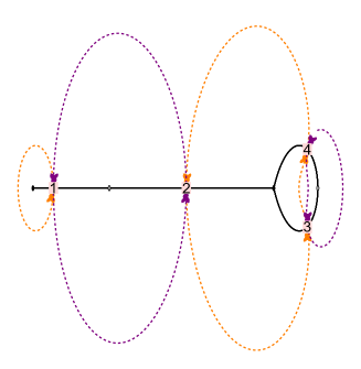
Figure 4.1: The dessin associated to $\Gamma_{0}(3)$ with passport $\{1^{1}3^{1},2^{2},1^{1}3^{1}\}$. Here, the numbers are the labels of the edges, and the orange (purple) cycles indicate the permutations around black (white) vertices.

It is then easy to see that the monodromy group $G$ is generated by $\sigma_{0}=\{(1),(234)\}$ and $\sigma_{1}=\{(12),(34)\}$. This is a subgroup of $\mathfrak{S}_{4}$ with $|G|=12$. From $\sigma_{\infty}\circ\sigma_{1}\circ\sigma_{0}=1$, we get $\sigma_{\infty}=\{(142)\}$.

Now for instance, let us choose a point on edge 2 as reference point. Then the monodromy for the $7$-brane associated to the internal face can be chosen to correspond to the permutation $\sigma^{a}=(234)$ while the (total) monodromy associated to the leftmost black vertex can be chosen to correspond to $\sigma^{b}=(12)$. As a result, the (total) monodromy for the $7$-branes associated to the external face is $\sigma^{c}=(2143)$ so that $\sigma^{c}\circ\sigma^{b}\circ\sigma^{a}=1$. It is obvious that $\sigma^{a}\in\sigma_{0}$, $\sigma^{b}\in\sigma_{1}$ and $\sigma^{c}=(\sigma^{b}\circ\sigma^{a})^{-1}$ all belong to $G$.

As the choice for $(p,q)$ is not unique, alternatively we may also choose for example $\sigma^{a}=(234)(34)=(23)$ and $\sigma^{b}=(12)$. Then $\sigma^{c}=(213)$.

A comment on F-theory on elliptically fibred K3

It is well-known that the compactification of F-theory on an elliptically fibred K3 surface is dual to heterotic string theory compactified on $\mathbb{T}^{2}$. In this setting, the elliptic fibre is still $y^{2}=x^{3}+f(k)x+g(k)$ with $k\in\mathbb{P}^{1}$, but now the degrees of $f$ and $g$ become 8 and 12 respectively. Hence, the number of 7-branes is 24. Although the graph consisting of edges connecting black and white vertices may not be a dessin or even be bipartite any more, the above discussions should still apply following similar methods.

4.2 Mahler Measure and Gromov-Witten Invariants

When the F-theory is compactified on one of our CY 3-folds, its effective theory is a closed subsector of the type II compactification. The BPS states of the F-theory compactification should then give a subsector of those in the full type II theory. In Klemm:1996hh ; Lerche:1996ni , such instanton expansions were computed. In particular, the GW invariants of local vanishing del Pezzo surfaces (independently of the global embedding in the CY spaces where F-theory compactifies) were observed to coincide with certain modular expansions of Mahler measures from the same toric diagrams later in Stienstra:2005wy . Here, we propose that the GW invariants of any vanishing 4-cycles could be recovered from such modular expansions from the corresponding toric diagrams according to the dictionary of the two sides.

As an elliptic curve is topologically $\mathbb{T}^{2}$, the periods are given by $\tilde{\phi}$ and $\tilde{\phi}_{D}$ following the notations of Lerche:1996ni . Then we shall identify the gauge coupling $\partial\tilde{\phi}_{D}/\partial\tilde{\phi}$ with $\tau$ on the modular Mahler measure side, that is,

$$\tau\sim\frac{\partial\tilde{\phi}_{D}}{\partial\tilde{\phi}}.$$ (4.7)

The instanton expansions in Lerche:1996ni are worked out at the large complex structure point $c=0$, where $c=\text{e}^{2\pi i\tilde{\phi}}+\dots$ provides a coordinate on the moduli space. This corresponds to the tropical limit $k\rightarrow\infty$, or equivalently, $q\rightarrow 0$. A natural ansatz for the correspondence would then be

$$c\sim q^{\nu}$$ (4.8)

for some $\nu\in\mathbb{Z}^{+}$.

In order to have the correspondence consistent, our goal is to show that this leads to the correspondence between the Yukawa coupling $C_{\tilde{\phi}\tilde{\phi}\tilde{\phi}}$ in Lerche:1996ni and $\frac{\text{d}\log q}{\text{d}m}$ in Stienstra:2005wy . In particular, they have the expansions

$$C_{\tilde{\phi}\tilde{\phi}\tilde{\phi}}=c_{0}+\sum_{n=1}^{\infty}\frac{\mathfrak{a}_{n}n^{3}q_{\tilde{\phi}}^{n}}{1-q_{\tilde{\phi}}^{n}},\quad\frac{\text{d}\log q}{\text{d}m}=-1+\sum_{n=1}^{\infty}\frac{a_{n}n^{3}(\text{e}^{-\nu m})^{n}}{1-(\text{e}^{-\nu m})^{n}},$$ (4.9)

where $q_{\tilde{\phi}}:=\text{e}^{2\pi i\tilde{\phi}}$ and $\nu$, $c_{0}$ are some positive constants depending on different cases. Then $a_{n}$ coincides with the GW invariants $\mathfrak{a}_{n}$ up to the constant $c_{0}$, that is, $\mathfrak{a}_{n}=-c_{0}a_{n}$.

Following these two expansions, we should have

$$\text{e}^{-\nu m}\sim q_{\tilde{\phi}}=\text{e}^{2\pi i\tilde{\phi}}.$$ (4.10)

Indeed, the expansion for $q^{\nu}$ is $q^{\nu}=\text{e}^{-\nu m}+\dots$, which agrees with $c=\text{e}^{2\pi i\tilde{\phi}}+\dots$. Now, since $m=-2\pi i\tau-\dots$, we have $m\sim-2\pi i\tau$. This would yield $\tilde{\phi}\sim\nu\tau$. As $u_{0}\sim 1$, we shall further tune the constant factor to be

$$\tilde{\phi}\sim-c_{0}\tau u_{0}.$$ (4.11)

The reason is that with

$$\tilde{\phi}_{D}\sim-\frac{1}{2\pi i}c_{0}\tau u_{1},$$ (4.12)

using $u_{1}\sim u_{0}\log\lambda\sim u_{0}\log q=2\pi i\tau u_{0}$, we can recover

$$\frac{\partial\tilde{\phi}_{D}}{\partial\tilde{\phi}}=\frac{\partial\tilde{\phi}_{D}/\partial\tau}{\partial\tilde{\phi}/\partial\tau}\sim\frac{1}{2\pi i}\frac{c_{0}\partial u_{1}/\partial\tau}{c_{0}u_{0}}=\tau.$$ (4.13)

Now we are ready to show that

$$C_{\tilde{\phi}\tilde{\phi}\tilde{\phi}}\sim-c_{0}\frac{\text{d}\log q}{\text{d}m},$$ (4.14)

where

$$C_{\tilde{\phi}\tilde{\phi}\tilde{\phi}}=\frac{\partial^{2}\tilde{\phi}_{D}}{\partial\tilde{\phi}^{2}}\sim\frac{\partial\tau}{\partial\tilde{\phi}}.$$ (4.15)

This can be seen as follows. Since $\lambda=q+\dots$, we have

$$-\frac{\text{d}m}{\text{d}\log q}=-\frac{\text{d}m}{\text{d}\log\lambda}=u_{0}.$$ (4.16)

On the other hand,

$$\frac{\partial\tilde{\phi}}{\partial\tau}\sim\frac{\partial(-c_{0}\tau u_{0})}{\partial\tau}=-c_{0}u_{0}.$$ (4.17)

Thus,

$$C_{\tilde{\phi}\tilde{\phi}\tilde{\phi}}\sim-\frac{1}{c_{0}u_{0}}\sim-c_{0}\frac{\text{d}\log q}{\text{d}m}.$$ (4.18)

Since we are working at the large complex structure point/tropical limit, “$\sim$” can be turned into “$=$”. To summarize, the correspondence of quantities between Mahler measure and GW invariants is listed in Table 4.1. This generalizes the observations in Stienstra:2005wy .

Mahler	$-c_{0}\tau u_{0}$	$-\frac{1}{4\pi i}c_{0}\tau u_{1}$	$\tau$	$q^{\nu}$	$\text{e}^{-\nu m}$	$-c_{0}\frac{\text{d}\log q}{\text{d}m}$
GW	$\tilde{\phi}$	$\tilde{\phi}_{D}$	$\partial\tilde{\phi}_{D}/\partial\tilde{\phi}$	$c$	$q_{\tilde{\phi}}$	$C_{\tilde{\phi}\tilde{\phi}\tilde{\phi}}$

Table 4.1: The correspondence between Mahler and GW in the tropical limit.

Outlook

Regarding the dictionary in Table 4.1, we expect that the correspondence between Mahler measure and GW invariants holds for all 16 reflexive polygons. It would be interesting to have a precise proof of the correspondence. Incidentally, the partition function on $S^{2}$ for certain gauged linear sigma model was used to compute genus-0 GW invariants for a 3d CY variety in Jockers:2012dk without the use of mirror symmetry. In particular, this linear sigma model flows an IR non-linear sigma model with the CY variety as the target space. It would be interesting to see whether modular Mahler measures could have any relations to this. Moreover, the dictionary between Mahler measure and GW invariants can be potentially extended to the topological vertex formalism.

By virtue of elliptic curves, the theories discussed in this section would have natural connections to Seiberg-Witten (SW) theories as pointed out in Lerche:1996ni ; Hori:2000ck . It is also worth noting that dessins have also appeared in the study of SW curves as in Ashok:2006br ; He:2015vua ; Bao:2021vxt . It could be possible that the discussions on dessins and (modular) Mahler measures in this paper would give some new insights to the study of SW theories and topological strings. From the perspective of (modular) Mahler measure, it would also be interesting to apply this to crystal melting, superconformal index, knot/quiver correspondence, black holes etc.

Appendix A Maximally and Minimally Tempered Newton Polynomials

In Table LABEL:Pzwmaxmin, we list all the maximally and minimally tempered Newton polynomials for the reflexive polygons.

Table A.1: The maximally and minimally tempered Newton polynomials for reflexive polygons.

Polygon	Maximally tempered polynomial	Minimally tempered polynomial
No.1	$k-\frac{w^{2}}{z}-\frac{z^{2}}{w}-\frac{3w}{z}-\frac{3z}{w}-\frac{1}{wz}-3w-\frac{3}{w}-3z-\frac{3}{z}$	$k-\frac{w^{2}}{z}-\frac{z^{2}}{w}-\frac{1}{wz}$
No.2	$k-\frac{w^{3}}{z}-\frac{4w^{2}}{z}-\frac{6w}{z}-\frac{z}{w}-\frac{1}{wz}-2w-\frac{2}{w}-\frac{4}{z}$	$k-\frac{w^{3}}{z}-\frac{z}{w}-\frac{1}{wz}$
No.3	$k-\frac{w^{2}}{z}-\frac{3w}{z}-\frac{z}{w}-\frac{1}{wz}-2w-\frac{2}{w}-z-\frac{3}{z}$	$k-\frac{w^{2}}{z}-\frac{z}{w}-\frac{1}{wz}-z$
No.4	$k-wz-\frac{z}{w}-\frac{w}{z}-\frac{1}{wz}-2w-\frac{2}{w}-2z-\frac{2}{z}$	$k-wz-\frac{z}{w}-\frac{w}{z}-\frac{1}{wz}$
No.5	$k-\frac{w^{2}}{z}-\frac{3w}{z}-\frac{1}{wz}-2w-\frac{1}{w}-z-\frac{3}{z}$	$k-\frac{w^{2}}{z}-\frac{1}{wz}-\frac{1}{w}-z$
No.6	$k-\frac{w^{2}}{z}-\frac{2w}{z}-\frac{z}{w}-2w-\frac{1}{w}-z-\frac{1}{z}$	$k-\frac{w^{2}}{z}-\frac{z}{w}-\frac{1}{w}-z-\frac{1}{z}$
No.7	$k-\frac{w^{2}}{z}-\frac{3w}{z}-\frac{1}{wz}-2w-z-\frac{3}{z}$	$k-\frac{w^{2}}{z}-\frac{1}{wz}-z$
No.8	$k-\frac{w^{2}}{z}-\frac{2w}{z}-2w-\frac{1}{w}-z-\frac{1}{z}$	$k-\frac{w^{2}}{z}-\frac{1}{w}-z-\frac{1}{z}$
No.9	$k-\frac{w}{z}-\frac{1}{wz}-w-\frac{1}{w}-z-\frac{2}{z}$	$k-\frac{w}{z}-\frac{1}{wz}-w-\frac{1}{w}-z$
No.10	$k-\frac{z}{w}-\frac{w}{z}-w-\frac{1}{w}-z-\frac{1}{z}$	$k-\frac{z}{w}-\frac{w}{z}-w-\frac{1}{w}-z-\frac{1}{z}$
No.11	$k-\frac{w}{z}-\frac{1}{wz}-\frac{1}{w}-z-\frac{2}{z}$	$k-\frac{w}{z}-\frac{1}{wz}-\frac{1}{w}-z$
No.12	$k-\frac{1}{wz}-w-\frac{1}{w}-z-\frac{1}{z}$	$k-\frac{1}{wz}-w-\frac{1}{w}-z-\frac{1}{z}$
No.13	$k-\frac{w}{z}-\frac{1}{wz}-z-\frac{2}{z}$	$k-\frac{w}{z}-\frac{1}{wz}-z$
No.14	$k-\frac{1}{wz}-w-\frac{1}{w}-z$	$k-\frac{1}{wz}-w-\frac{1}{w}-z$
No.15	$k-w-\frac{1}{w}-z-\frac{1}{z}$	$k-w-\frac{1}{w}-z-\frac{1}{z}$
No.16	$k-z-w-\frac{1}{zw}$	$k-z-w-\frac{1}{zw}$

Appendix B Elliptic Curves for Minimally Tempered Coefficients

Although not as physically interesting as the maximally tempered coefficients, let us list the results for minimally tempered coefficients for comparison and reference. As the reflexive polygons No.10, 12, 14, 15 and 16 do not have any boundary points other than vertices, the minimally tempered coefficients coincide with the maximially tempered coefficients. Hence, we will not repeat their results here.

As shown in Table LABEL:ellipticminimally, the elliptic curves for minimally tempered coefficients are not the same for specular duals. The reason is that these coefficients do not encode all the information of the corresponding (numbers of) perfect matchings.

Table B.1: The data of the elliptic curves $y^{2}=x^{3}+fx+g$ and $j$-invariants for reflexive polygons (with minimally tempered coefficients). Again, we have $f=-\frac{1}{48}k^{4}+a(k)$ and $g=\frac{1}{864}k^{6}+b(k)$ here.

Polygon	No.1	No.2	No.3	No.4
$a(k)$	$-\frac{9}{2}k$	$-4$	$-3$	$\frac{1}{3}k^{2}-\frac{16}{3}$
$b(k)$	$-\frac{5}{8}k^{3}-\frac{27}{4}$	$-\frac{2}{3}k^{2}$	$-\frac{3}{4}k^{2}-2$	$-\frac{1}{36}k^{4}-\frac{4}{9}k^{2}+\frac{128}{27}$
$j(k)$	$\frac{k^{3}(k^{3}+216)^{3}}{(k^{3}-27)^{3}}$	$\frac{(k^{4}+192)^{3}}{(k^{4}-64)^{2}}$	$\frac{(k^{4}+144)^{3}}{k^{2}(k^{2}-16)(k^{2}+9)^{2}}$	$\frac{(k^{4}-16k^{2}+256)^{3}}{k^{4}(k^{2}-16)^{2}}$
Polygon	No.5		No.6
$a(k)$	$1$		$\frac{1}{6}k^{2}+\frac{1}{2}k+\frac{5}{3}$
$b(k)$	$-\frac{1}{12}k^{2}-k-1$		$-\frac{1}{72}k^{4}-\frac{1}{24}k^{3}-\frac{1}{9}k^{2}-\frac{5}{6}k-\frac{125}{108}$
$j(k)$	$\frac{(k^{4}-48)^{3}}{k^{7}+k^{6}+k^{4}-72k^{3}-504k^{2}-864k-496}$		$\frac{(k^{4}-8k^{2}-24k-80)^{3}}{(k^{2}+4k+5)^{2}(k^{3}-6k^{2}+12k-35)}$
Polygon	No.7	No.8	No.9
$a(k)$	$0$	$\frac{1}{2}k^{2}+k$	$\frac{1}{6}k^{2}+k+\frac{2}{3}$
$b(k)$	$-1$	$-\frac{1}{24}k^{4}-\frac{1}{12}k^{3}+\frac{1}{4}k^{2}+k+1$	$-\frac{1}{72}k^{4}-\frac{1}{12}k^{3}-\frac{1}{36}k^{2}+\frac{1}{3}k-\frac{7}{27}$
$j(k)$	$\frac{k^{12}}{k^{6}-432}$	$\frac{(k^{4}-8k^{2}-32)^{3}}{k^{6}-11k^{4}-32k^{2}-256}$	$\frac{(k^{4}-8k^{2}-48k-32)^{3}}{(k+1)^{2}(k^{4}-8k^{2}-64k-48)}$
Polygon	No.11		No.13
$a(k)$	$\frac{1}{2}k+1$		$1$
$b(k)$	$-\frac{1}{24}k^{3}-\frac{1}{12}k^{2}+\frac{1}{4}$		$-\frac{1}{12}k^{2}$
$j(k)$	$\frac{(k^{4}-24k-48)^{3}}{k^{5}+k^{4}+k^{3}-30k^{2}-96k-91}$		$\frac{(k^{4}-48)^{3}}{k^{4}-64}$

In Figure B.1, we list the plots obtained from $j(k)/1728$. As we can see, this is not a Belyi map for No.8, and hence the plot is not dessin or even a bipartite graph. Moreover, although the graph for No.9 is bipartite, it is not connected, and hence the map is not Belyi as well.

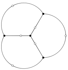
(a) No.1: $\Gamma(3)$

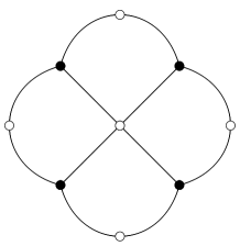
(b) No.2

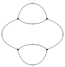
(c) No.3: $\Gamma_{0}(4)\cap\Gamma(2)$

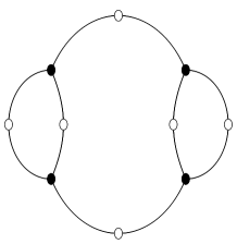
(d) No.4: $\Gamma_{0}(4)\cap\Gamma(2)$

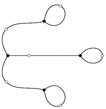
(e) No.5: $\Gamma_{0}(9)$

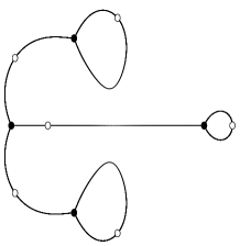
(f) No.6: $\Gamma_{0}(9)$

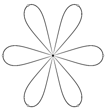
(g) No.7

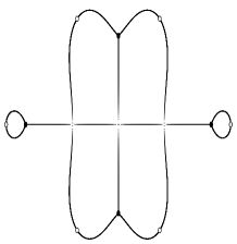
(h) No.8

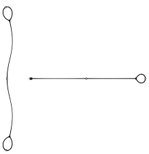
(i) No.9: $\Gamma_{0}(3)\times\Gamma_{0}(4)$

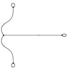
(j) No.11: $\Gamma_{0}(9)$

(k) No.13

Figure B.1: The dessins (or just graphs from $j/1728$) for reflexive polygons with minimally tempered coefficients. As listed, some of them correspond to certain congruence subgroups (as coset graphs).

One may also compute the Mahler measures for the Newton polynomials $P(z,w)=k-p(z,w)$ with those minimally tempered coefficients as series of $k$. We will not list them here, but we would like to point out two properties:

• There are several (but not all) reflexive pairs giving the same Mahler measures. These pairs are No.1&16, No.2&13, No.4&15 (plus the self-dual ones). The reason is that the vertices of the polygons in each pair are related by some GL$(2,\mathbb{Z})$ transformation (while the other reflexive duals are not). This can be seen by quotient gradings on the lattice or directly computations of Plücker coordinates. As the minimally tempered coefficients only contain the vertices, this then follows from the fact that Mahler measure is GL$(2,\mathbb{Z})$ invariant.

• There are four classes of polygons whose Mahler measures can be expressed compactly using some generalized hypergeometric functions ${}_{4}F_{3}$. Likewise, their $u_{0}$ are also simply some hypergeometric functions ${}_{2}F_{1}$. These four classes are classified in villegas1999modular . It turns out that the four classes are precisely No.1&16, No.2&13, No.4&15 and the self-dual No.7.

Although not all dessins (or just graphs) are associated to congruence subgroups, we may still compute the modular expansions for the $k$ parameters and check if they give rise to any Hauptmoduln. Here we give three examples of different types. The detailed steps can be found in Stienstra:2005wy ; samart2014mahler .

Example 1: No.1

As this is the same as the case for dP₀ (No.16), we have computed that $k^{3}=27+\left(\frac{\eta(\tau)}{\eta(3\tau)}\right)^{12}$. This is a Hauptmodul for $\Gamma_{0}(3)$. In particular, the congruence subgroup associated to the dessin in this case is $\Gamma(3)$, which is a subgroup of $\Gamma_{0}(3)$.

Example 2: No.11

We have

$$k^{4}=q^{-1}+40+276q-2048q^{2}+11202q^{3}+\dots=64+\left(\frac{\eta(\tau)}{\eta(2\tau)}\right)^{24},$$ (B.1)

where the second equality is checked perturbatively. This is a Hauptmodul for $\Gamma_{0}(2)$. On the other hand, the crossing dessin does not correspond to any congruence subgroup. By removing the white vertices (or black vertices), this does not even seem to be a coset graph for any group either.

Example 3: No.7

We have

$$k^{6}=864\left(1-\frac{E_{6}(\tau)}{E_{4}^{3/2}(\tau)}\right),$$ (B.2)

where $E_{4}(\tau)=1+240\sum\limits_{n=1}^{\infty}\frac{n^{3}q^{n}}{1-q^{n}}$ and $E_{6}(\tau)=1-540\sum\limits_{n=1}^{\infty}\frac{n^{5}q^{n}}{1-q^{n}}$ are the Eisenstein series. This is not known to be a Hauptmodul of any genus-0 congruence subgroup. On the other hand, the flower dessin does not correspond to any congruence subgroup either. By removing the white vertices, however, it could be viewed as a coset graph associated to any group with 6 generators (and the subgroup being itself). Incidentally, there are two things worth noting:

• As given in FrickeKlein , we have

  $$E_{4}^{1/4}(\tau)={}_{2}F_{1}\left(\frac{1}{12},\frac{5}{12};1;\frac{1728}{j}\right)$$ (B.3)

  in terms of $j$-invariant (cf. §3.2).

• The $q$-series expansion for $E_{4}(\tau)$ has $a_{n}=240$ for $n\geq 1$. It turns out that $2a_{n}=480$ are the GW invariants in the first row of Table 1 given in Klemm:1996hh (cf. §4.2).

References

- (1) K. Mahler, “On some inequalities for polynomials in several variables,” Journal of the London Mathematical Society 1 no. 1, (1962) 341–344.
- (2) D. W. Boyd, “Speculations concerning the range of mahler’s measure,” Canadian Mathematical Bulletin 24 no. 4, (1980) 453–469.
- (3) D. W. Boyd, “Kronecker’s theorem and lehmer’s problem for polynomials in several variables,” Journal of Number Theory 13 no. 1, (1981) 116–121.
- (4) F. R. Villegas, “Modular mahler measures i,” in Topics in number theory, pp. 17–48. Springer, 1999.
- (5) D. W. Boyd, F. Rodriguez-Villegas, and N. M. Dunfield, “Mahler’s measure and the dilogarithm (ii),” arXiv:math/0308041.
- (6) M.-J. Bertin and M. Lalín, “Mahler measure of multivariable polynomials,” Women in numbers 2: research directions in number theory 606 (2013) 125–147.
- (7) D. W. Boyd, “Mahler’s measure and invariants of hyperbolic manifolds,” Number theory for the millennium, I (Urbana, IL, 2000) (2002) 127–143.
- (8) R. Dijkgraaf and H. Fuji, “The Volume Conjecture and Topological Strings,” Fortsch. Phys. 57 (2009) 825–856, arXiv:0903.2084 [hep-th].
- (9) R. Kenyon, A. Okounkov, and S. Sheffield, “Dimers and amoebae,” arXiv:math-ph/0311005.
- (10) H. Ooguri and M. Yamazaki, “Emergent Calabi-Yau Geometry,” Phys. Rev. Lett. 102 (2009) 161601, arXiv:0902.3996 [hep-th].
- (11) J. Stienstra, “Mahler measure, Eisenstein series and dimers,” in Workshop on Calabi-Yau Varieties and Mirror Symmetry, pp. 151–158. 2, 2005. arXiv:math/0502197.
- (12) A. Zahabi, “Toric Quiver Asymptotics and Mahler Measure: BPS States,” JHEP 07 (2019) 121, arXiv:1812.10287 [hep-th].
- (13) A. Zahabi, “Thermodynamics of Isoradial Quivers and Hyperbolic 3-Manifolds,” Int. J. Mod. Phys. A 35 no. 20, (2020) 2050105, arXiv:1912.13245 [hep-th].
- (14) A. Zahabi, “Quiver asymptotics and amoeba: Instantons on toric Calabi-Yau divisors,” Phys. Rev. D 103 no. 8, (2021) 086024, arXiv:2006.14041 [hep-th].
- (15) J. Bao, Y.-H. He, and A. Zahabi, “Mahler Measure for a Quiver Symphony,” arXiv:2108.13903 [hep-th].
- (16) E. Girondo and G. González-Diez, Introduction to compact Riemann surfaces and dessins d’enfants, vol. 79. Cambridge University Press, 2012.
- (17) A. Grothendieck, “Esquisse d’un Programme,” 1984.
- (18) G. Belyi, “On galois extensions of a maximal cyclotomic field,” Mathematics of the USSR-Izvestiya 14 no. 2, (1980) 247.
- (19) Y.-H. He, J. McKay, and J. Read, “Modular Subgroups, Dessins d’Enfants and Elliptic K3 Surfaces,” LMS J. Comp. Math. 16 (2013) 271–318, arXiv:1211.1931 [math.AG].
- (20) Y.-H. He and J. Read, “Hecke Groups, Dessins d’Enfants and the Archimedean Solids,” Front. in Phys. 3 (2015) 91, arXiv:1309.2326 [math.AG].
- (21) Y.-H. He and J. Read, “Dessins d’enfants in generalised quiver theories,” JHEP 08 (2015) 085, arXiv:1503.06418 [hep-th].
- (22) V. Tatitscheff, Y.-H. He, and J. McKay, “Cusps, Congruence Groups and Monstrous Dessins,” arXiv:1812.11752 [math.NT].
- (23) Y.-H. He, E. Hirst, and T. Peterken, “Machine-learning dessins d’enfants: explorations via modular and Seiberg–Witten curves,” J. Phys. A 54 no. 7, (2021) 075401, arXiv:2004.05218 [hep-th].
- (24) S. K. Ashok, F. Cachazo, and E. Dell’Aquila, “Children’s drawings from Seiberg-Witten curves,” Commun. Num. Theor. Phys. 1 (2007) 237–305, arXiv:hep-th/0611082.
- (25) J. Stienstra, “Hypergeometric Systems in two Variables, Quivers, Dimers and Dessins d’Enfants,” Fields Inst. Commun. 54 (2008) 125–162, arXiv:0711.0464 [math.AG].
- (26) V. Jejjala, S. Ramgoolam, and D. Rodriguez-Gomez, “Toric CFTs, Permutation Triples and Belyi Pairs,” JHEP 03 (2011) 065, arXiv:1012.2351 [hep-th].
- (27) S. Bose, J. Gundry, and Y.-H. He, “Gauge theories and dessins d‘enfants: beyond the torus,” JHEP 01 (2015) 135, arXiv:1410.2227 [hep-th].
- (28) J. Bao, O. Foda, Y.-H. He, E. Hirst, J. Read, Y. Xiao, and F. Yagi, “Dessins d’enfants, Seiberg-Witten curves and conformal blocks,” JHEP 05 (2021) 065, arXiv:2101.08843 [hep-th].
- (29) S. Franco, A. Hanany, K. D. Kennaway, D. Vegh, and B. Wecht, “Brane dimers and quiver gauge theories,” JHEP 01 (2006) 096, arXiv:hep-th/0504110.
- (30) S. Franco, A. Hanany, D. Martelli, J. Sparks, D. Vegh, and B. Wecht, “Gauge theories from toric geometry and brane tilings,” JHEP 01 (2006) 128, arXiv:hep-th/0505211.
- (31) B. Feng, Y.-H. He, K. D. Kennaway, and C. Vafa, “Dimer models from mirror symmetry and quivering amoebae,” Adv. Theor. Math. Phys. 12 no. 3, (2008) 489–545, arXiv:hep-th/0511287.
- (32) M. Kontsevich and D. Zagier, “Periods,” in Mathematics unlimited—2001 and beyond, pp. 771–808. Springer, 2001.
- (33) A. Hanany, Y.-H. He, V. Jejjala, J. Pasukonis, S. Ramgoolam, and D. Rodriguez-Gomez, “Invariants of Toric Seiberg Duality,” Int. J. Mod. Phys. A 27 (2012) 1250002, arXiv:1107.4101 [hep-th].
- (34) Y.-H. He, V. Jejjala, and D. Rodriguez-Gomez, “Brane Geometry and Dimer Models,” JHEP 06 (2012) 143, arXiv:1204.1065 [hep-th].
- (35) W. Lerche, P. Mayr, and N. P. Warner, “Noncritical strings, Del Pezzo singularities and Seiberg-Witten curves,” Nucl. Phys. B 499 (1997) 125–148, arXiv:hep-th/9612085.
- (36) A. Klemm, P. Mayr, and C. Vafa, “BPS states of exceptional noncritical strings,” Nucl. Phys. B Proc. Suppl. 58 (1997) 177, arXiv:hep-th/9607139.
- (37) J. Stienstra, “Mahler measure variations, Eisenstein series and instanton expansions,” in Workshop on Calabi-Yau Varieties and Mirror Symmetry, pp. 139–150. 2, 2005. arXiv:math/0502193.
- (38) J. Stienstra, “Motives from diffraction,” in Annual EAGER Conference 2004: Workshop Algebraic Cycles and Motives. 11, 2005. arXiv:math/0511485.
- (39) W. Fulton, Introduction to Toric Varieties.(AM-131), Volume 131. Princeton university press, 2016.
- (40) D. A. Cox, J. B. Little, and H. K. Schenck, Toric varieties, vol. 124. American Mathematical Soc., 2011.
- (41) K. Hori and C. Vafa, “Mirror symmetry,” arXiv:hep-th/0002222.
- (42) A. Hanany and R.-K. Seong, “Brane Tilings and Reflexive Polygons,” Fortsch. Phys. 60 (2012) 695–803, arXiv:1201.2614 [hep-th].
- (43) T. Shioda, “On elliptic modular surfaces,” Journal of the Mathematical Society of Japan 24 no. 1, (1972) 20–59.
- (44) Y.-H. He and J. McKay, “N=2 Gauge Theories: Congruence Subgroups, Coset Graphs and Modular Surfaces,” J. Math. Phys. 54 (2013) 012301, arXiv:1201.3633 [hep-th].
- (45) B. Feng, A. Hanany, and Y.-H. He, “D-brane gauge theories from toric singularities and toric duality,” Nucl. Phys. B 595 (2001) 165–200, arXiv:hep-th/0003085.
- (46) A. Hanany and K. D. Kennaway, “Dimer models and toric diagrams,” arXiv:hep-th/0503149.
- (47) R. Kenyon, “An introduction to the dimer model,” arXiv:math/0310326.
- (48) A. Hanany and R.-K. Seong, “Brane Tilings and Specular Duality,” JHEP 08 (2012) 107, arXiv:1206.2386 [hep-th].
- (49) D. Forcella, A. Hanany, Y.-H. He, and A. Zaffaroni, “Mastering the Master Space,” Lett. Math. Phys. 85 (2008) 163–171, arXiv:0801.3477 [hep-th].
- (50) D. Forcella, A. Hanany, Y.-H. He, and A. Zaffaroni, “The Master Space of N=1 Gauge Theories,” JHEP 08 (2008) 012, arXiv:0801.1585 [hep-th].
- (51) J. Bao, G. Beaney Colverd, and Y.-H. He, “Quiver Gauge Theories: Beyond Reflexivity,” JHEP 20 (2020) 161, arXiv:2004.05295 [hep-th].
- (52) Y.-H. He, R.-K. Seong, and S.-T. Yau, “Calabi–Yau Volumes and Reflexive Polytopes,” Commun. Math. Phys. 361 no. 1, (2018) 155–204, arXiv:1704.03462 [hep-th].
- (53) J. Davey, A. Hanany, and J. Pasukonis, “On the Classification of Brane Tilings,” JHEP 01 (2010) 078, arXiv:0909.2868 [hep-th].
- (54) A. Hanany, V. Jejjala, S. Ramgoolam, and R.-K. Seong, “Consistency and Derangements in Brane Tilings,” J. Phys. A 49 no. 35, (2016) 355401, arXiv:1512.09013 [hep-th].
- (55) W. Stein et al., Sage Mathematics Software (Version x.y.z). The Sage Development Team, YYYY. http://www.sagemath.org.
- (56) E. Goins, “Drawing Planar Graphs via Dessins d’Enfants,” 2013.
- (57) D. Samart, Mahler measures of hypergeometric families of Calabi-Yau varieties. PhD thesis, 2014.
- (58) D. Zagier, “Integral solutions of apéry-like recurrence equations,” Groups and Symmetries: from Neolithic Scots to John McKay, CRM Proc. Lecture Notes 47 (2009) 349–366.
- (59) G. Diaz, “Mahler’s conjecture and other transcendence results,” in Introduction to Algebraic Independence Theory, pp. 13–26. Springer, 2001.
- (60) A. Hanany, Y.-H. He, V. Jejjala, J. Pasukonis, S. Ramgoolam, and D. Rodriguez-Gomez, “The Beta Ansatz: A Tale of Two Complex Structures,” JHEP 06 (2011) 056, arXiv:1104.5490 [hep-th].
- (61) K. Hori, A. Iqbal, and C. Vafa, “D-branes and mirror symmetry,” arXiv:hep-th/0005247.
- (62) A. Sen, “F theory and orientifolds,” Nucl. Phys. B 475 (1996) 562–578, arXiv:hep-th/9605150.
- (63) A. Sen, “Orientifold limit of F theory vacua,” Phys. Rev. D 55 (1997) R7345–R7349, arXiv:hep-th/9702165.
- (64) M. R. Gaberdiel, T. Hauer, and B. Zwiebach, “Open string-string junction transitions,” Nucl. Phys. B 525 (1998) 117–145, arXiv:hep-th/9801205.
- (65) H. Jockers, V. Kumar, J. M. Lapan, D. R. Morrison, and M. Romo, “Two-Sphere Partition Functions and Gromov-Witten Invariants,” Commun. Math. Phys. 325 (2014) 1139–1170, arXiv:1208.6244 [hep-th].
- (66) F. Klein and R. Fricke, Lectures on the Theory of Elliptic Modular Functions.