Towards Calibrated Model for Long-Tailed Visual Recognition from Prior Perspective

Abstract

Real-world data universally confronts a severe class-imbalance problem and exhibits a long-tailed distribution, i.e., most labels are associated with limited instances. The naïve models supervised by such datasets would prefer dominant labels, encounter a serious generalization challenge and become poorly calibrated. We propose two novel methods from the prior perspective to alleviate this dilemma. First, we deduce a balance-oriented data augmentation named Uniform Mixup (UniMix) to promote mixup in long-tailed scenarios, which adopts advanced mixing factor and sampler in favor of the minority. Second, motivated by the Bayesian theory, we figure out the Bayes Bias (Bayias), an inherent bias caused by the inconsistency of prior, and compensate it as a modification on standard cross-entropy loss. We further prove that both the proposed methods ensure the classification calibration theoretically and empirically. Extensive experiments verify that our strategies contribute to a better-calibrated model and their combination achieves state-of-the-art performance on CIFAR-LT, ImageNet-LT, and iNaturalist 2018.

1 Introduction

Balanced and large-scaled datasets [53, 42] have promoted deep neural networks to achieve remarkable success in many visual tasks [25, 52, 23]. However, real-world data typically exhibits a long-tailed (LT) distribution [37, 45, 28, 19], and collecting a minority category (tail) sample always leads to more occurrences of common classes (head) [57, 29], resulting in most labels associated with limited instances. The paucity of samples may cause insufficient feature learning on the tail classes [69, 14, 36, 45], and such data imbalance will bias the model towards dominant labels [56, 57, 40]. Hence, the generalization of minority categories is an enormous challenge.

The intuitive approaches such as directly over-sampling the tail [11, 6, 48, 54, 7] or under-sampling the head [20, 6, 22] will cause serious robustness problems. mixup [64] and its extensions [59, 63, 12] are effective feature improvement methods and contribute to a well-calibrated model in balanced datasets [58, 65], i.e., the predicted confidence indicates actual accuracy likelihood [18, 58]. However, mixup is inadequately calibrated in an imbalanced LT scenario (Fig.1). In this paper, we raise a conception called $\xi$-Aug to analyze mixup and figure out that it tends to generate more head-head pairs, resulting in unsatisfactory generalization of the tail. Therefore, we propose Uniform Mixup (UniMix), which adopts a tail-favored mixing factor related to label prior and a inverse sampling strategy to encourage more head-tail pairs occurrence for better generalization and calibration.

Previous works adjust the logits weight [34, 14, 56, 62] or margin [8, 47] on standard Softmax cross-entropy (CE) loss to tackle the bias towards dominant labels. We analyze the inconstancy of label prior, which varies in LT train set and balanced test set, and pinpoint an inherent bias named Bayes Bias (Bayias). Based on the Bayesian theory, the posterior is proportional to prior times likelihood. Hence, it’s necessary to adjust the posterior on train set by compensating different prior for each class, which can serve as an additional margin on CE. We further demonstrate that the Bayias-compensated CE ensures classification calibration and propose a unified learning manner to combine Bayias with UniMix towards a better-calibrated model (see in Fig.1). Furthermore, we suggest that bad calibrated approaches are counterproductive with each other, which provides a heuristic way to analyze the combined results of different feature improvement and loss modification methods (see in Tab.4).

In summary, our contributions are: 1) We raise the concept of $\xi$-Aug to theoretically explain the reason of mixup’s miscalibration in LT scenarios and propose Unimix (Sec.3.1) composed of novel mixing and sampling strategies to construct a more class-balanced virtual dataset. 2) We propose the Bayias (Sec.3.2) to compensate the bias incurred by different label prior, which can be unified with UniMix by a training manner for better classification calibration. 3) We conduct sufficient experiments to demonstrate that our method trains a well-calibrated model and achieves state-of-the-art results on CIFAR-10-LT, CIFAR-100-LT, ImageNet-LT, and iNaturalist 2018.

figurec

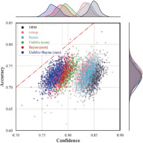
Figure 1: Joint density plots of accuracy vs. confidence to measure the calibration of classifiers on CIFAR-100-LT-100 during training. A well-calibrated classifier’s density will lay around the red dot line $y=x$, indicating prediction score reflects the actual likelihood of accuracy. mixup manages to regularize classifier on balanced datasets. However, both mixup and its extensions tend to be overconfident in LT scenarios. Our UniMix reconstructs a more balanced dataset and Bayias-compensated CE erases prior bias to ensure better calibration. Without loss of accuracy, either of proposed methods trains the same classifier more calibrated and their combination achieves the best. How to measure calibration and more visualization results are available in Appendix D.2.

2 Analysis of mixup

The core of supervised image classification is to find a $\theta$ parameterized mapping $\mathcal{F}_{\theta}:X\in\mathds{R}^{c\times h\times w}\mapsto Y\in\mathds{R}^{C\times 1}$ to estimate the empirical Dirac delta distribution $\mathds{P}_{\delta}(x,y)=\frac{1}{N}\sum\nolimits_{i=1}^{N}\delta(x_{i},y_{i})$ of $N$ instances $x\in\mathcal{X}$ and labels $y\in\mathcal{Y}$. The learning progress by minimizing Eq.1 is known as Empirical Risk Minimization (ERM), where $\mathcal{L}(Y=y_{i},\mathcal{F}_{\theta}(X=x_{i}))$ is $x_{i}$’s conditional risk.

$$R_{\delta}(\mathcal{F}_{\theta})=\int_{x\in\mathcal{X}}\mathcal{L}\left(Y=y,\mathcal{F}_{\theta}(X=x)\right)d\mathds{P}_{\delta}(x,y)=\frac{1}{N}\sum\nolimits_{i=1}^{N}\mathcal{L}\left(Y=y_{i},\mathcal{F}_{\theta}(X=x_{i})\right)$$ (1)

To overcome the over-fitting caused by insufficient training of $N$ samples, mixup utilizes Eq.2 to extend the feature space to its vicinity based on Vicinal Risk Minimization (VRM) [10].

$$\widetilde{x}=\xi\cdot x_{i}+(1-\xi)\cdot x_{j}\qquad\widetilde{y}=\xi\cdot y_{i}+(1-\xi)\cdot y_{j}$$ (2)

where $\xi\sim Beta(\alpha,\alpha),\alpha\in[0,1]$, the sample pair $(x_{i},y_{i}),(x_{j},y_{j})$ is drawn from training dataset $\mathcal{D}_{train}$ randomly. Hence, Eq.2 converts $\mathds{P}_{\delta}(X,Y)$ into empirical vicinal distribution $\mathds{P}_{\nu}(\widetilde{x},\widetilde{y})=\frac{1}{N}\sum\nolimits_{i=1}^{N}\nu(\widetilde{x},\widetilde{y}|x_{i},y_{i})$, where $\nu(\cdot)$ describes the manner of finding virtual pairs $(\widetilde{x},\widetilde{y})$ in the vicinity of arbitrary sample $(x_{i},y_{i})$. Then, we construct a new dataset $\mathcal{D}_{\nu}:=\{(\widetilde{x}_{k},\widetilde{y}_{k})\}_{k=1}^{M}$ via Eq.2 and minimize the empirical vicinal risk by Vicinal Risk Minimization (VRM):

$$R_{\nu}(\mathcal{F}_{\theta})=\int_{\widetilde{x}\in\widetilde{\mathcal{X}}}\mathcal{L}\left(\widetilde{{Y}}=\widetilde{y},\mathcal{F}_{\theta}(\widetilde{{X}}=\widetilde{x})\right)d\mathds{P}_{\nu}(\widetilde{x},\widetilde{y})=\frac{1}{M}\sum\nolimits_{i=1}^{M}\mathcal{L}\left(\widetilde{{Y}}=\widetilde{y}_{i},\mathcal{F}_{\theta}(\widetilde{{X}}=\widetilde{x}_{i})\right)$$ (3)

mixup is proven to be effective on balanced dataset due to its improvement of calibration [58, 18], but it is unsatisfactory in LT scenarios (see in Tab.4). In Fig.1, mixup fails to train a calibrated model, which surpasses baseline (ERM) a little in accuracy and seldom contributes to calibration (far from $y=x$). To analyze the insufficiency of mixup, the definition of $\xi$-Aug is raised.

Definition 1

$\xi$-Aug. The virtual sample $(\widetilde{x}_{i,j},\widetilde{y}_{i,j})$ generated by Eq.2 with mixing factor $\xi$ is defined as a $\xi$-Aug sample, which is a robust sample of class $y_{i}$ $($class $y_{j})$ iff $\xi\geq 0.5(\xi<0.5)$ that contributes to class $y_{i}$ (class $y_{j}$) in model’s feature learning.

In LT scenarios, we reasonably assume the instance number $n$ of each class is exponential with parameter $\lambda$ [14] if indices are descending sorted by $n_{y_{i}}$, where $y_{i}\in[1,C]$ and $C$ is the total class number. Generally, the imbalance factor is defined as $\rho=n_{y_{1}}/n_{y_{C}}$ to measure how skewed the LT dataset is. It is easy to draw $\lambda=\ln\rho/(C-1)$. Hence, we can describe the LT dataset as Eq.4:

$$\mathds{P}(Y=y_{i})=\frac{{\iint_{x_{i}\in\mathcal{X},y_{j}\in\mathcal{Y}}{\mathds{1}(X=x_{i},Y=y_{i})dx_{i}dy_{j}}}}{{\iint_{{x_{i}}\in\mathcal{X},{y_{j}}\in\mathcal{Y}}{\mathds{1}(X={x_{i}},Y={y_{j}})dx_{i}dy_{j}}}}=\frac{\lambda}{e^{-\lambda}-e^{-\lambda C}}{e^{-\lambda y_{i}}},y_{i}\in[1,C]$$ (4)

Then, we derive the following corollary to illustrate the limitation of naïve mixup strategy.

Corollary 1

When $\bm{\xi\sim Beta(\alpha,\alpha)},\alpha\in[0,1]$, the newly mixed dataset $\mathcal{D}_{\nu}$ composed of $\xi$-Aug samples $(\widetilde{x}_{i,j},\widetilde{y}_{i,j})$ follows the same long-tailed distribution as the origin dataset $\mathcal{D}_{train}$, where $(x_{i},y_{i})$ and $(x_{j},y_{j})$ are randomly sampled from $\mathcal{D}_{train}$. (See detail derivation in Appendix A.2.)

$$\mathds{P}_{\textit{mixup}}(Y^{*}={y_{i}}) =\mathds{P}^{2}(Y={y_{i}})+\mathds{P}(Y={y_{i}})\iint_{y_{i}\neq y_{j}}{Beta(\alpha,\alpha)}\mathds{P}(Y={y_{j}})d\xi dy_{j}$$ (5)

$$=\frac{\lambda}{e^{-\lambda}-e^{-\lambda C}}{e^{-\lambda y_{i}}},y_{i}\in[1,C]$$

In mixup, the probability of any $(\widetilde{x}_{i,j},\widetilde{y}_{i,j})$ belongs to class $y_{i}$ or class $y_{j}$ is strictly determined by $\xi$ and $\mathds{E}(\xi)\equiv 0.5$. Furthermore, both $(x_{i},y_{i})$ and $(x_{j},y_{j})$ are randomly sampled and concentrated on the head instead of tail, resulting in that the head classes get more $\xi$-Aug samples than the tail ones.

3 Methodology

3.1 UniMix: balance-oriented feature improvement

mixup and its extensions tend to generate head-majority pseudo data, which leads to the deficiency on the tail feature learning and results in a bad-calibrated model. To obtain a more balanced dataset $\mathcal{D}_{\nu}$, we propose the UniMix Factor $\xi^{*}_{i,j}$ related to the prior probability of each category and a novel UniMix Sampler to obtain sample pairs. Our motivation is to generate comparable $\xi$-Aug samples of each class for better generalization and calibration.

UniMix Factor.

Specifically, the prior in imbalanced train set and balanced test set of class $y_{i}$ is defined as $\mathds{P}_{train}(Y=y_{i})\triangleq\pi_{y_{i}}$, and $\mathds{P}_{test}(Y=y_{i})\equiv 1/C$, respectively. We design the UniMix Factor $\xi_{i,j}^{*}$ for each virtual sample $\widetilde{x}_{i,j}$ instead of a fixed $\xi$ in mixup. Consider adjusting $\xi$ with the class prior probability $\pi_{y_{i}},\pi_{y_{j}}$. It is intuitive that a proper factor $\xi_{i,j}=\pi_{y_{j}}/(\pi_{y_{i}}+\pi_{y_{j}})$ ensures $\widetilde{x}_{i,j}$ to be a $\xi$-Aug sample of class $y_{j}$ if $\pi_{y_{i}}\geq\pi_{y_{j}}$, i.e., class $y_{i}$ occupies more instances than class $y_{j}$.

However, $\xi_{i,j}$ is uniquely determined by $\pi_{y_{i}},\pi_{y_{j}}$. To improve the robustness and generalization, original $Beta(\alpha,\alpha)$ is adjusted to obtain UniMix Factor $\xi_{i,j}^{*}$. Notice that $\xi$ is close to $0$ or $1$ and symmetric at $0.5$, we transform it to maximize the probability of $\xi_{i,j}=\pi_{y_{j}}/(\pi_{y_{i}}+\pi_{y_{j}})$ and its vicinity. Specifically, if note $\xi\sim Beta(\alpha,\alpha)$ as $f(\xi;\alpha,\alpha)$, we define $\xi_{i,j}^{*}\sim\mathscr{U}(\pi_{y_{i}},\pi_{y_{j}},\alpha,\alpha)$ as:

$$\xi_{i,j}^{*}\sim\mathscr{U}(\pi_{y_{i}},\pi_{y_{j}},\alpha,\alpha)=\left\{\begin{aligned} &f(\xi_{i,j}^{*}-\frac{\pi_{y_{j}}}{\pi_{y_{i}}+\pi_{y_{j}}}+1;\alpha,\alpha),&\xi_{i,j}^{*}\in[0,\frac{\pi_{y_{j}}}{\pi_{y_{i}}+\pi_{y_{j}}});\\ &f(\xi_{i,j}^{*}-\frac{\pi_{y_{j}}}{\pi_{y_{i}}+\pi_{y_{j}}};\alpha,\alpha),&\xi_{i,j}^{*}\in[\frac{\pi_{y_{j}}}{\pi_{y_{i}}+\pi_{y_{j}}},1]\end{aligned}\right.$$ (6)

Rethink Eq.2 with $\xi_{i,j}^{*}$ described as Eq.6:

$$\widetilde{x}_{i,j}=\xi_{i,j}^{*}\cdot x_{i}+(1-\xi_{i,j}^{*})\cdot x_{j}\qquad\widetilde{y}_{i,j}=\xi_{i,j}^{*}\cdot y_{i}+(1-\xi_{i,j}^{*})\cdot y_{j}$$ (7)

We have the following corollary to show how $\xi^{*}_{i,j}$ ameliorates the imbalance of $\mathcal{D}_{train}$:

Corollary 2

When $\bm{\xi_{i,j}^{*}\sim\mathscr{U}(\pi_{y_{i}},\pi_{y_{j}},\alpha,\alpha)},\alpha\in[0,1]$, the newly mixed dataset $\mathcal{D}_{\nu}$ composed of $\xi$-Aug samples $(\widetilde{x}_{i,j},\widetilde{y}_{i,j})$ follows a middle-majority distribution (see Fig.2), where $(x_{i},y_{i})$ and $(x_{j},y_{j})$ are both randomly sampled from $\mathcal{D}_{train}$. (See detail derivation in Appendix A.3.)

$$\mathds{P}_{\textit{mixup}}^{*}(Y^{*}={y_{i}}) =\mathds{P}(Y={y_{i}})\int_{y_{j}<{y_{i}}}{\mathds{1}\left(\int{\xi^{*}_{i,j}\mathscr{U}(\pi_{i},\pi_{j},\alpha,\alpha)d\xi^{*}_{i,j}\geq 0.5}\right)\mathds{P}(Y={y_{j}})dy_{j}}$$ (8)

$$=\frac{\lambda}{{{{\left({{e^{-\lambda}}-{e^{-\lambda C}}}\right)}^{2}}}}\left({{e^{-\lambda\left({{y_{i}}+1}\right)}}-{e^{-2\lambda{y_{i}}}}}\right),y_{i}\in[1,C]$$

UniMix Sampler.

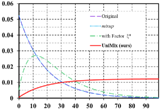
Figure 2: Visualization of $\xi$-Aug samples distribution ($C=100,\rho=200$) in Corollary1,2,3. $x$-axis: class indices. $y$-axis: probability of each class. mixup (blue) exhibits the same LT distribution as origin (purple). $\xi^{*}$ (green) alleviates such situation and the full pipeline ($\tau=-1$) (red) constructs a more uniform distributed dataset. See more results in Appendix A.5.

UniMix Factor facilitates $\xi$-Aug samples more balance-distributed over all classes. However, most samples are still $\xi$-Aug for the head or middle (see Fig.2(green)). Actually, the constraint that pair $x_{i},x_{j}$ drawn from the head and tail respectively is preferred, which dominantly generates $\xi$-Aug samples for tail classes with $\xi_{i,j}^{*}$. To this end, we consider sample $x_{j}$ from $\mathcal{D}_{train}$ with probability inverse to the label prior:

$${\mathds{P}_{inv}}(Y={y_{i}})=\frac{{\mathds{P}^{\tau}(Y={y_{i}})}}{{\int_{{y_{j}}\in\mathcal{Y}}{\mathds{P}^{\tau}(Y={y_{j}})dy_{j}}}}$$ (9)

When $\tau=1$, UniMix Sampler is equivalent to a random sampler. $\tau<1$ indicates that $x_{j}$ has higher probability drawn from tail class. Note that $x_{i}$ is still randomly sampled from $\mathcal{D}_{train}$, i.e., it’s most likely drawn from the majority class. The virtual sample $\widetilde{x}_{i,j}$ obtained in this manner is mainly a $\xi$-Aug sample of the tail composite with $x_{i}$ from the head. Hence Corollary3 is derived:

Corollary 3

When $\bm{\xi_{i,j}^{*}\sim\mathscr{U}(\pi_{y_{i}},\pi_{y_{j}},\alpha,\alpha)},\alpha\in[0,1]$, the newly mixed dataset $\mathcal{D}_{\nu}$ composed of $\xi$-Aug samples $(\widetilde{x}_{i,j},\widetilde{y}_{i,j})$ follows a tail-majority distribution (see Fig.2), where $(x_{i},y_{i})$ is randomly and $(x_{j},y_{j})$ is inversely sampled from $\mathcal{D}_{train}$, respectively. (See detail derivation in Appendix A.4.)

$${\mathds{P}_{UniMix}}({Y^{*}}={y_{i}}) =\mathds{P}(Y={y_{i}})\int_{y_{j}<{y_{i}}}{\mathds{1}\left(\int{\xi^{*}_{i,j}\mathscr{U}(\pi_{i},\pi_{j},\alpha,\alpha)d\xi^{*}_{i,j}\geq 0.5}\right)\mathds{P}_{inv}(Y=y_{j})dy_{j}}$$ (10)

$$=\frac{\lambda}{{\left({{e^{-\lambda}}-{e^{-\lambda C}}}\right)\left({{e^{-\lambda\tau C}}-{e^{-\lambda\tau}}}\right)}}\left({{e^{-\lambda{y_{i}}\left({\tau+1}\right)}}-{e^{-\lambda\left({\tau+{y_{i}}}\right)}}}\right),y_{i}\in[1,C]$$

With the proposed UniMix Factor and UniMix Sampler, we get the complete UniMix manner, which constructs a uniform $\xi$-Aug samples distribution for VRM and greatly facilitates model’s calibration (See Fig.2 (red) & 1). We construct $\mathcal{D}_{\nu}:=\{(\widetilde{x}_{k},\widetilde{y}_{k})\}_{k=1}^{M}$ where $\{\widetilde{x}_{k},\widetilde{y}_{k}\}$ is $(\widetilde{x}_{i,j},\widetilde{y}_{i,j})$ generated by $(x_{i},y_{i})$ and $(x_{j},y_{j})$. We conduct training via Eq.3 and the loss via VRM is available as:

$$\mathcal{L}(\widetilde{y}_{k},\mathcal{F}_{\theta}(\widetilde{x}_{k}))=\xi_{i,j}^{*}\mathcal{L}(y_{i},\mathcal{F}_{\theta}(\widetilde{x}_{i,j}))+(1-\xi_{i,j}^{*})\mathcal{L}(y_{j},\mathcal{F}_{\theta}(\widetilde{x}_{i,j}))$$ (11)

3.2 Bayias: an inherent bias in LT

The bias between LT set and balanced set is ineluctable and numerous studies [14, 57, 61] have demonstrated its existence. To eliminate the systematic bias that classifier tends to predict the head, we reconsider the parameters training process. Generally, a classifier can be modeled as:

$$\hat{y}=\mathop{\arg\max}_{y_{i}\in\mathcal{Y}}\frac{e^{\sum\nolimits_{{d_{i}}\in D}[{{{({W^{T}})_{{y_{i}}}^{({d_{i}})}\mathcal{F}{{(x;\theta)}^{(d_{i})}}]+{b_{{y_{i}}}}}}}}}{{\sum\nolimits_{{y_{j}}\in\mathcal{Y}}e^{\sum\nolimits_{{d_{i}}\in D}[{{{({W^{T}})_{{y_{j}}}^{({d_{i}})}\mathcal{F}{{(x;\theta)}^{(d_{i})}}]+{b_{{y_{j}}}}}}}}}}\triangleq\mathop{\arg\max}_{y_{i}\in\mathcal{Y}}\frac{{{e^{\psi{{(x;\theta,W,b)}_{{y_{i}}}}}}}}{{\sum\nolimits_{{y_{j}}\in\mathcal{Y}}{{e^{\psi{{(x;\theta,W,b)}_{{y_{j}}}}}}}}}$$ (12)

where $\hat{y}$ indicts the predicted label, and $\mathcal{F}(x;\theta)\in\mathds{R}^{D\times 1}$ is the $D$-dimension feature extracted by the backbone with parameter $\theta$. $W\in\mathds{R}^{D\times C}$ represents the parameter matrix of the classifier.

Previous works [14, 57] have demonstrated that it is not suitable for imbalance learning if one ignores such bias. In LT scenarios, the instances number in each class of the train set varies greatly, which means the corresponding prior probability $\mathds{P}_{train}(Y=y)$ is highly skewed whereas the distribution on the test set $\mathds{P}_{test}(Y=y)$ is uniform.

According to Bayesian theory, posterior is proportional to prior times likelihood. The supervised training process of $\psi(x;\theta,W,b)$ in Eq.12 can regard as the estimation of likelihood, which is equivalent to get posterior for inference in balanced dataset. Considering the difference of prior during training and testing, we have the following theorem (See detail derivation in Appendix B.1):

Theorem 3.1

For classification, let $\psi(x;\theta,W,b)$ be a hypothesis class of neural networks of input $X=x$, the classification with Softmax should contain the influence of prior, i.e., the predicted label during training should be:

$$\hat{y}=\mathop{\arg\max}_{y_{i}\in\mathcal{Y}}\frac{{{e^{\psi{{(x;\theta,W,b)}_{{y_{i}}}}+\bm{\log(\pi_{y_{i}})+\log(C)}}}}}{{\sum\nolimits_{{y_{j}}\in\mathcal{Y}}{{e^{\psi{{(x;\theta,W,b)}_{{y_{j}}}}+\bm{\log(\pi_{y_{j}})+\log(C)}}}}}}$$ (13)

In balanced datasets, all classes share the same prior. Hence, the supervised model $\psi(x;\theta,W,b)$ could use the estimated likelihood $\mathds{P}(X=x|Y=y)$ of train set to correctly obtain posterior $\mathds{P}(Y=y|X=x)$ in test set. However, in LT datasets where $\mathds{P}_{train}(Y=y_{i})=\pi_{y_{i}}$ and $\mathds{P}_{test}(Y=y_{i})\equiv 1/C$, prior cannot be regard as a constant over all classes any more. Due to the difference on prior, the learned parameters $\theta,W,b\triangleq\Theta$ will yield class-level bias, i.e., the optimization direction is no longer as described in Eq.12. Thus, the bias incurred by prior should compensate at first. To correctness the bias for inferring, the offset term that model in LT dataset to compensate is:

$$\mathscr{B}_{y}=\log(\pi_{y})+\log(C)$$ (14)

Furthermore, the proposed Bayias $\mathscr{B}_{y}$ enables predicted probability reflecting the actual correctness likelihood, expressed as Theorem 3.2. (See detail derivation in Appendix B.2.)

Theorem 3.2

$\mathscr{B}_{y}$-compensated cross-entropy loss in Eq.15 ensures classification calibration.

$$\mathcal{L}_{\mathscr{B}}(y_{i},\psi(x;\Theta))=\log\left[1+\sum\nolimits_{y_{k}\neq y_{i}}e^{(\mathscr{B}_{y_{k}}-\mathscr{B}_{y_{i}})}\cdot e^{\psi(x;\Theta)_{y_{k}}-\psi(x;\Theta)_{y_{i}}}\right]$$ (15)

Here, the optimization direction during training will convert to $\psi(X;\theta,W,b)+\mathscr{B}_{y}$. In particular, if the train set is balanced, $\mathds{P}_{train}(Y=y)\triangleq\pi_{y}\equiv 1/C$, then $\mathscr{B}_{y}=\log(1/C)+\log(C)\equiv 0$, which means the Eq.12 is a balanced case of Eq.13. We further raise that $\mathscr{B}_{y}$ is critical to the classification calibration in Theorem 3.2. The pairwise loss in Eq.15 will guide model to avoid over-fitting the tail or under-fitting the head with better generalization, which contributes to a better calibrated model.

Compared with logit adjustment [47], which is also a margin modification, it is necessary to make a clear statement about the concrete difference from three points. 1) Logit adjustment is motivated by Balanced Error Rate (BER), while the Bayias compensated CE loss is inspired by the Bayesian theorem. We focus more on the model performance on the real-world data distribution. 2) As motioned above, our loss is consistent with standard CE loss when the train set label prior is the same as real test label distribution. 3) Our loss can tackle the imbalanced test set situation as well by simply setting the margin as $\mathscr{B}_{y}=\log(\pi_{y})+\log(\pi^{\prime}_{y})$, where the $\pi^{\prime}_{y}$ represents the test label distribution. The experiment evidence can be found in Appendix Tab.D2.

3.3 Towards calibrated model with UniMix and Bayias

Algorithm 1 Integrated training manner towards calibrated model.

0:  $\mathcal{D}_{train}$, Batch Size $\mathcal{N}$, Stop Steps $T_{1},T_{2}$, Random Sampler $\mathcal{R}$, UniMix Sampler $\mathcal{R}^{*}$

0:  Optimized $\Theta^{*}$, i.e., feature extractor parameters $\theta^{*}$, classifier parameters $W^{*},b^{*}$

1:  Initialize the parameters $\Theta^{(0)}$ randomly and calculate $\mathscr{B}_{y}$ via Eq.14

2:  for $t=0$ to $T_{1}$ do

3:     Sample a mini-batch $\mathcal{B}=\{x_{i},y_{i}\}_{i=1}^{\mathcal{N}}\leftarrow\mathcal{R}(\mathcal{D}_{train},\mathcal{N})$

4:     Sample a mini-batch $\mathcal{B}^{*}=\{x_{j}^{*},y_{j}^{*}\}_{j=1}^{\mathcal{N}}\leftarrow\mathcal{R^{*}}(\mathcal{D}_{train},\mathcal{N})$

5:     Calculate UniMix factor $\xi^{*}$ via Eq.6

6:     Construct VRM dataset $\mathcal{B}_{\nu}=\{\widetilde{x}_{k},\widetilde{y}_{k}\}_{k=1}^{\mathcal{N}}$ via Eq.7

7:     Calculate $\mathcal{L}_{\mathcal{B_{\nu}}}=\mathds{E}[\xi^{*}_{i,j}\mathcal{L}_{\mathscr{B}}(y_{i},\psi(\widetilde{x};\Theta^{(t)}))+(1-\xi^{*}_{i,j})\mathcal{L}_{\mathscr{B}}(y^{*}_{j},\psi(\widetilde{x};\Theta^{(t)}))]$ via Eq.11,15

8:     Update $\Theta^{(t+1)}\leftarrow\Theta^{(t)}-\alpha\nabla_{\Theta^{(t)}}\mathcal{L}_{\mathcal{B_{\nu}}}$

9:  end for

10:  for $t=T_{1}$ to $T_{2}$ do

11:     Sample a mini-batch $\mathcal{B}=\{x_{i},y_{i}\}_{i=1}^{\mathcal{N}}\leftarrow\mathcal{R}(\mathcal{D}_{train},\mathcal{N})$

12:     Calculate $\mathcal{L}_{\mathcal{B}}=\mathds{E}[\mathcal{L}_{\mathscr{B}}(y_{i},\psi(x_{i};\Theta))]$ via Eq.15

13:     Update $\Theta^{(t+1)}\leftarrow\Theta^{(t)}-\alpha\nabla_{\Theta^{(t)}}\mathcal{L}_{\mathcal{B}}$

14:  end for

It’s intuitive to integrate feature improvement methods with loss modification ones for better performance. However, we find such combinations fail in most cases and are counterproductive with each other, i.e., the combined methods reach unsatisfactory performance gains. We suspect that these methods take contradictory trade-offs and thus result in overconfidence and bad calibration. Fortunately, the proposed UniMix and Bayias are both proven to ensure calibration. To achieve a better-calibrated model for superior performance gains, we introduce Alg.1 to tackle the previous dilemma and integrate our two proposed approaches to deal with poor generalization of tail classes. Specially, inspired by previous work [26], we overcome the coverage difficulty in mixup [64] by removing UniMix in the last several epochs and thus maintain the same epoch as baselines. Note that Bayias-compensated CE is only adopted in the training process as discussed in Sec.3.2.

4 Experiment

4.1 Results on synthetic dataset

We make an ideal binary classification using Support Vector Machine (SVM) [16] to show the distinguish effectiveness of UniMix. Suppose there are samples from two disjoint circles respectively:

$$z^{+}=\{(x,y)|(x-x_{0})^{2}+(y-y_{0})^{2}\leq r^{2}\}$$ (16)

$$z^{-}=\{(x,y)|(x+x_{0})^{2}+(y+y_{0})^{2}\leq r^{2}\}$$

To this end, we randomly sample $m$ discrete point pairs from $z^{+}$ to compose positive samples $z^{+}_{p}=\{(x^{+}_{1},y^{+}_{1}),\cdots,(x^{+}_{m},y^{+}_{m})\}$, and $m$ negative samples $z^{-}_{n}=\{(x^{-}_{1},y^{+}_{1}),\cdots,(x^{-}_{m},y^{-}_{m})\}$ from $z^{-}$ correspondingly, thus to generate a balanced dataset $\mathcal{D}_{bal}=\{z^{+}_{p},z^{-}_{n}\}$ with $\mathds{P}\left((x,y)\in z^{+}_{p}\right)=\mathds{P}\left((x,y)\in z^{-}_{n}\right)=0.5$. For imbalance data, we sample $n(n\ll m)$ negative data from $z^{-}$ to generate $z^{-}_{n^{\prime}}=\{(x^{\prime-}_{1},y^{\prime-}_{1}),\cdots,(x^{\prime-}_{n},y^{\prime-}_{n})\}$, so as to compose the imbalance dataset $\mathcal{D}_{imbal}=\{z^{+}_{p},z^{-}_{n^{\prime}}\}$, with $\mathds{P}\left((x,y)\in z^{+}_{p}\right)\gg\mathds{P}\left((x,y)\in z^{-}_{n^{\prime}}\right)$. We train the SVM model on the two synthetic datasets, and visualize the classification boundary of each dataset in Fig.3.

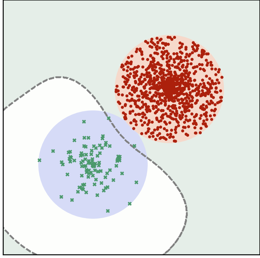
(a) imbalanced scenario

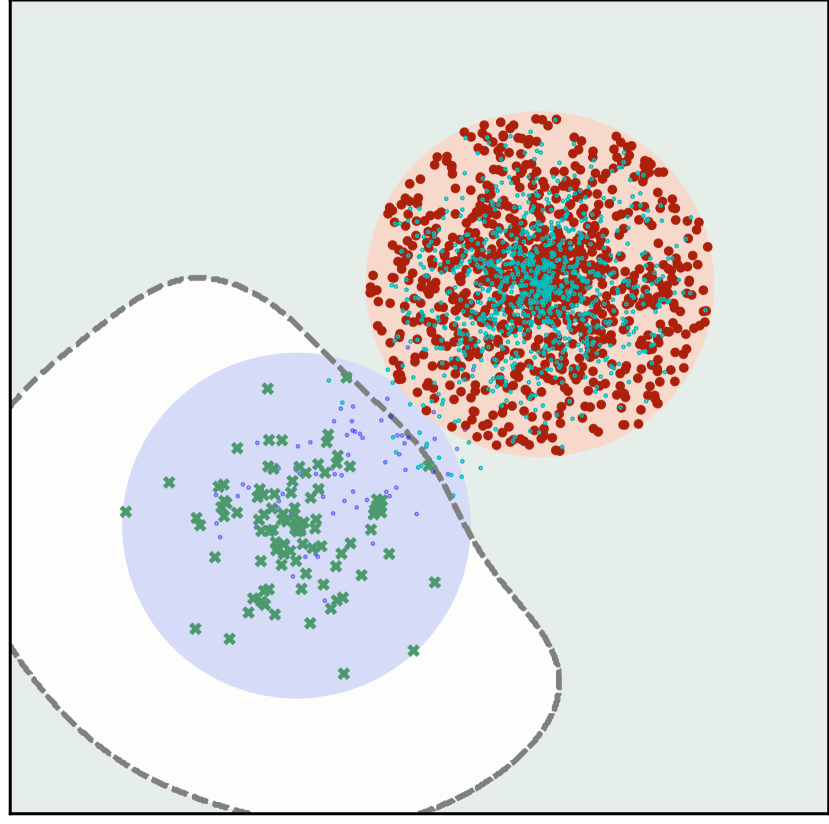
(b) with mixup

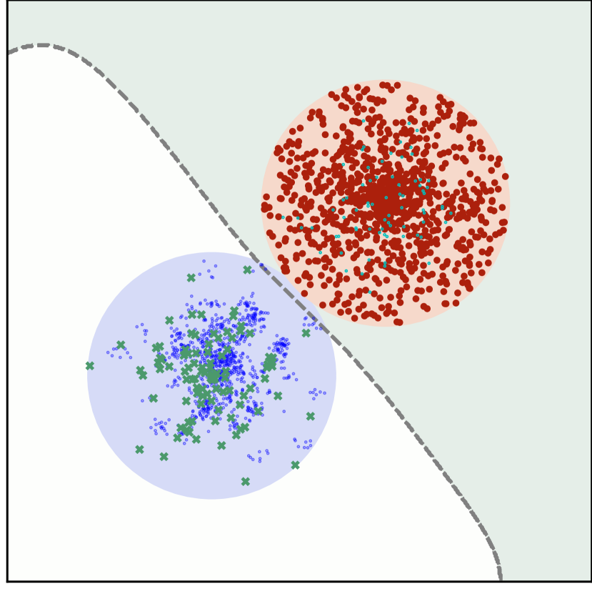
(c) with UniMix

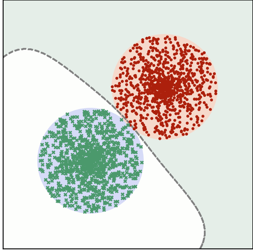
(d) balanced scenario

Figure 3: SVM decision boundary on the synthetic balanced dataset (Fig.3(d)) and imbalanced dataset (Fig.3(a),3(b),3(c)). The theoretical classification boundary of the synthetic dataset is $y$=$-x$. "$\circ$" represents generated pseudo data, where blue and green represent belong to $z^{-}$ and $z^{+}$, respectively.

The SVM reaches an approximate ideal boundary on balanced datasets (Fig.3(d)) but severely deviates from the $y=-x$ in the imbalanced dataset (Fig.3(a)). As proven in Sec.2, mixup (Fig.3(b)) is incapable of shifting imbalance distribution, resulting in no better result than the original one (Fig.3(a)). After adopting the proposed UniMix, the classification boundary in Fig.3(c) shows much better results than the original imbalanced dataset, which gets closed to the ideal boundary.

4.2 Results on CIFAR-LT

The imbalanced datasets CIFAR-10-LT and CIFAR-100-LT are constructed via suitably discarding training samples following previous works [69, 14, 47, 8]. The instance numbers exponentially decay per class in train dataset and keep balanced during inference. We extensively adopt $\rho\in\{10,50,100,200\}$ for comprehensive comparisons. See implementation details in Appendix C.1.

Comparison methods. We evaluate the proposed method against various representative and effective approaches extensively, summarized into the following groups: a) Baseline. We conduct plain training with CE loss called ERM as baseline. b) Feature improvement methods modify the input feature to cope with LT datasets. mixup [64] convexly combines images and labels to build virtual data for VRM. Manifold mixup [59] performs the linear combination in latent states. Remix [12] conducts the same combination on images and adopts tail-favored rules on labels. M2m [36] converts majority images to minority ones by adding noise perturbation, which need an additional pre-trained classifier. BBN [69] utilizes features from two branches in a cumulative learning manner. c) Loss modification methods either adjust the logits weight or margin before the Softmax operation. Specifically, focal loss [41], CB [14] and CDT [62] re-weight the logits with elaborate strategies, while LDAM [8] and Logit Adjustment [47] add the logits margin to shift decision boundary away from tail classes. d) Other methods. We also compare the proposed method with other two-stage approaches (e.g. DRW [8]) for comprehensive comparisons.

Table 1: Top-1 validation accuracy(%) of ResNet-32 on CIFAR-10/100-LT. E2E: end to end training. Underscore: the best performance in each group. $\dagger$: our reproduced results. $\ddagger$: reported results in [69]. $\star$: reported results in [62]. Our calibration ensured method achieves the best performance.

Dataset	E2E	CIFAR-10-LT				CIFAR-100-LT
$\rho$ (easy $\rightarrow$ hard)	-	10	50	100	200	10	50	100	200
ERM†	✓	86.39	74.94	70.36	66.21	55.70	44.02	38.32	34.56
mixup‡ [64]	✓	87.10	77.82	73.06	67.73	58.02	44.99	39.54	34.97
Manifold Mixup‡ [59]	✓	87.03	77.95	72.96	-	56.55	43.09	38.25	-
Remix [12]	✓	88.15	79.20	75.36	67.08	59.36	46.21	41.94	36.99
M2m [36]	✗	87.90	-	78.30	-	58.20	-	42.90	-
BBN‡ [69]	✗	88.32	82.18	79.82	-	59.12	47.02	42.56	-
Focal⋆ [41]	✓	86.55	76.71†	70.43	65.85	55.78	44.32†	38.41	35.62
Urtasun et al [51]	✓	82.12	76.45	72.23	66.25	52.12	43.17	38.90	33.00
CB-Focal [14]	✓	87.10	79.22	74.57	68.15	57.99	45.21	39.60	36.23
$\tau$-norm⋆ [33]	✓	87.80	82.78†	75.10	70.30	59.10	48.23†	43.60	39.30
LDAM† [8]	✓	86.96	79.84	74.47	69.50	56.91	46.16	41.76	37.73
LDAM+DRW† [8]	✗	88.16	81.27	77.03	74.74	58.71	47.97	42.04	38.45
CDT⋆ [62]	✓	89.40	81.97†	79.40	74.70	58.90	45.15†	44.30	40.50
Logit Adjustment [47]	✓	89.26†	83.38†	79.91	75.13†	59.87†	49.76†	43.89	40.87†
Ours	✓	89.66	84.32	82.75	78.48	61.25	51.11	45.45	42.07

Results. We present results of CIFAR-10-LT and CIFAR-100-LT in Tab.1. Our proposed method achieves state-of-the-art results against others on each $\rho$, with performance gains improved as $\rho$ gets increased (See Appendix D.1). Specifically, our method overcomes the ignorance in tail classes effectively with better calibration, which integrates advantages of two group approaches and thus surpass most two-stage methods (i.e., BBN, M2m, LDAM+DRW). However, not all combinations can get ideal performance gains as expected. More details will be discussed in Sec.4.4.

Table 2: Quantitative calibration metric of ResNet-32 on CIFAR-10/100-LT test set. Smaller ECE and MCE indicate better calibration results. Either of the proposed methods achieves a well-calibrated model compared with others. The combination of UniMix and Bayias achieves the best performance.

Dataset	CIFAR-10-LT				CIFAR-100-LT
$\rho$	10		100		10		100
Calibration Metric (%)	ECE	MCE	ECE	MCE	ECE	MCE	ECE	MCE
ERM	6.60	74.96	20.53	73.91	22.85	34.50	38.23	87.22
mixup [64]	6.55	24.54	19.20	37.84	19.69	38.53	32.72	50.46
Remix [12]	6.81	22.44	15.38	27.99	20.17	32.99	33.56	50.96
LDAM+DRW [8]	11.22	45.92	19.89	49.07	30.54	55.57	42.18	64.78
UniMix (ours)	6.00	25.99	12.87	28.30	19.38	33.40	27.12	41.46
Bayias (ours)	5.52	20.14	11.05	23.72	17.42	28.26	24.31	39.66
UniMix+Bayias (ours)	4.74	13.67	10.19	25.47	15.24	23.67	23.04	37.36

To quantitatively describe the contribution to model calibration, we make quantitative comparisons on CIFAR-10-LT and CIFAR-100-LT. According to the definition ECE and MCE (see Appendix Eq.D.2,D.3), a well-calibrated model should minimize the ECE and MCE for better generalization and robustness. In this experiment, we adopt the most representative $\rho\in\{10,100\}$ with previous mainstream state-of-the-art methods.

The results in Tab.2 show that either of the proposed methods generally outperforms previous methods, and their combination enables better classification calibration with smaller ECE and MCE. Specifically, mixup and Remix have negligible contributions to model calibration. As analyzed before, such methods tend to generate head-head pairs in favor of the feature learning of majority classes. However, more head-tail pairs are required for better feature representation of the tail classes. In contrast, both the proposed UniMix and Bayias pay more attention to the tail and achieve satisfactory results. It is worth mentioning that improving calibration in post-hoc manners [18, 68] is also effective, and we will discuss it in Appendix D.2.3. Note that LDAM is even worse calibrated compared with baseline. We suggest that LDAM adopts an additional margin only for the ground-truth label from the angular perspective, which shifts the decision boundary away from the tail class and makes the tail predicting score tend to be larger. Additionally, LDAM requires the normalization of input features and classifier weight matrix. Although a scale factor is proposed to enlarge the logits for better Softmax operation [60], it is still harmful to calibration. It also accounts for its contradiction with other methods. Miscalibration methods combined will make models become even more overconfident and damage the generalization and robustness severely.

4.3 Results on large-scale datasets

We further verify the proposed method’s effectiveness quantitatively on large-scale imbalanced datasets, i.e. ImageNet-LT and iNaturalist 2018. ImageNet-LT is the LT version of ImageNet [53] by sampling a subset following Pareto distribution, which contains about $115K$ images from $1,000$ classes. The number of images per class varies from $5$ to $1,280$ exponentially, i.e., $\rho=256$. In our experiment, we utilize the balanced validation set constructed by Cui et al. [14] for fair comparisons. The iNaturalist species classification dataset [28] is a large-scale real-world dataset which suffers from extremely label LT distribution and fine-grained problems [28, 69]. It is composed of $435,713$ images over $8,142$ classes with $\rho=500$. The official splits of train and validation images [8, 69, 33] are adopted for fair comparisons. See implementation details in Appendix C.2.

Table 3: Top-1 validation accuracy(%) of ResNet-10/50 on ImageNet-LT and ResNet-50 on iNaturalist 2018. E2E: end to end training. $\dagger$: our reproduced results. $\ddagger$: results reported in origin paper.

Dataset	ImageNet-LT					iNaturalist 2018
Method	E2E	ResNet-10	$\Delta$	ResNet-50	$\Delta$	ResNet-50	$\Delta$
CE†	✓	35.88	-	38.88	-	60.88	-
CB-CE† [14]	✓	37.06	+1.18	40.85	+1.97	63.50	+2.62
LDAM [8]	✓	36.05†	+0.17	41.86†	+2.98	64.58‡	+3.70
OLTR‡ [45]	✗	35.60	-0.28	40.36	+1.48	63.90	+3.02
LDAM+DRW [8]	✗	38.22†	+2.34	45.75†	+6.87	68.00‡	+7.12
BBN‡ [69]	✗	-		-		66.29	+5.41
c-RT [33]	✗	41.80‡	+5.92	47.54†	+8.66	67.60†	+6.72
Ours	✓	42.90	+7.02	48.41	+9.53	69.15	+8.27

Results. Tab.3 illustrates the results on large-scale datasets. Ours is consistently effective and outperforms existing mainstream methods, achieving distinguish improvement compared with previous SOTA c-RT [33] in the compared backbones. Especially, our method outperforms the baseline on ImageNet-LT and iNaturalist 2018 by 9.53% and 8.27% with ResNet-50, respectively. As can be noticed in Tab.3, the proposed method also surpasses the well-known two-stage methods [33, 8, 69], achieving superior accuracy with less computation load in a concise training manner.

4.4 Further Analysis

Effectiveness of UniMix and Bayias. We conduct extensive ablation studies in Tab.4 to demonstrate the effectiveness of the proposed UnixMix and Bayias, with detailed analysis in various combinations of feature-wise and loss-wise methods on CIFAR-10-LT and CIFAR-100-LT. Indeed, both UniMix and Bayias turn out to be effective in LT scenarios. Further observation shows that with calibration ensured, the proposed method gets significant performance gains and achieve state-of-the-art results. Noteworthy, LDAM [8] makes classifiers miscalibrated, which leads to unsatisfactory improvement when combined with mixup manners.

Table 4: Ablation study between feature-wise and loss-wise methods. LDAM is counterproductive to mixup and its extensions. Bayias-compensated CE ensures calibration and shows excellent performance gains especially combined with UniMix.

Dataset		CIFAR-10-LT				CIFAR-100-LT
$\rho$ (easy $\rightarrow$ hard)		100		200		100		200
Mix	Loss	Top1 Acc	$\Delta$	Top1 Acc	$\Delta$	Top1 Acc	$\Delta$	Top1 Acc	$\Delta$
None	CE	70.36	-	66.21	-	38.32	-	34.56	-
mixup	CE	73.06	+2.70	67.73	+1.52	39.54	+1.22	34.97	+0.41
Remix	CE	75.36	+5.00	67.08	+0.87	41.94	+3.62	36.99	+2.43
UniMix	CE	76.47	+6.11	68.42	+2.21	41.46	+3.14	37.63	+3.07
None	LDAM	74.47	-	69.50	-	41.76	-	37.73	-
mixup	LDAM	73.96	-0.15	67.89	-1.61	40.22	-1.54	37.52	-0.21
Remix	LDAM	74.33	-0.14	69.66	+0.16	40.59	-1.17	37.66	-0.07
UniMix	LDAM	75.35	+0.88	70.77	+1.27	41.67	-0.09	37.83	+0.01
None	Bayias	78.70	-	74.21	-	43.52	-	38.83	-
mixup	Bayias	81.75	+3.05	76.69	+2.48	44.56	+1.04	41.19	+2.36
Remix	Bayias	81.55	+2.85	75.81	+1.60	45.01	+1.49	41.44	+2.61
UniMix	Bayias	82.75	+4.05	78.48	+4.27	45.45	+1.93	42.07	+3.24

Evaluating different UniMix Sampler. Corollary 1,2,3 demonstrate distinguish influence of UniMix. However, the $\xi$-sample can not be completely equivalent with orginal ones. Hence, an appropriate $\tau$ in Eq.9 is also worth further searching. Fig.4 illustrates the accuracy with different $\tau$ on CIFAR-10-LT and CIFAR-100-LT setting $\rho=10$ and $100$. For CIFAR-10-LT (Fig.4(a),4(b)), $\tau=-1$ is possibly ideal, which forces more head-tail instead of head-head pairs get generated to compensate tail classes. In the more challenging CIFAR-100-LT, $\tau=0$ achieves the best result. We suspect that unlike simple datasets (e.g., CIFAR-10-LT), where overconfidence occurs in head classes, all classes need to get enhanced in complicated LT scenarios. Hence, the augmentation is effective and necessary both on head and tail. $\tau=0$ allows both head and tail get improved simultaneously.

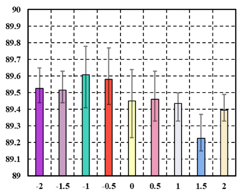
(a) CIFAR-10-LT-10.

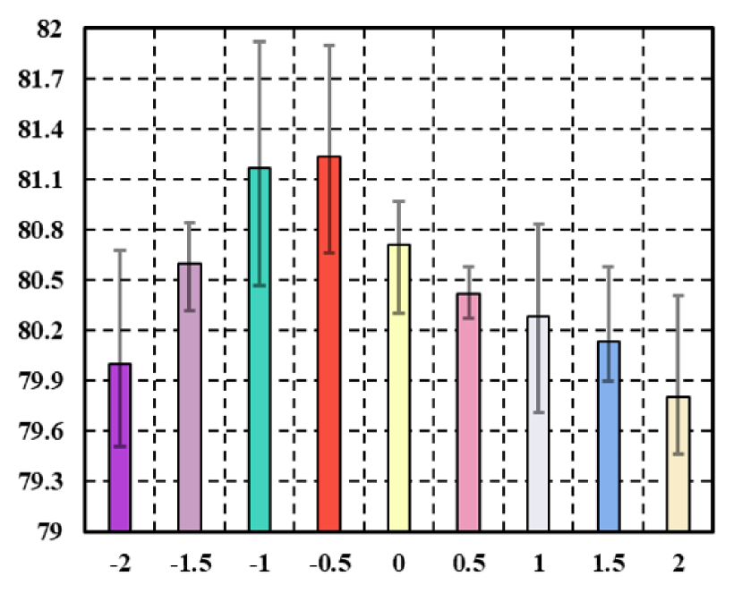
(b) CIFAR-10-LT-100.

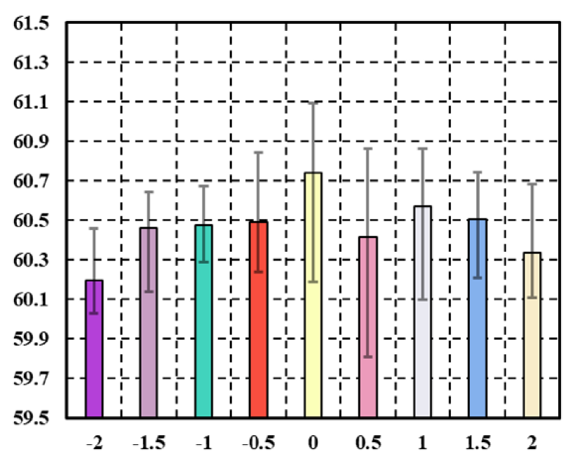
(c) CIFAR-100-LT-10.

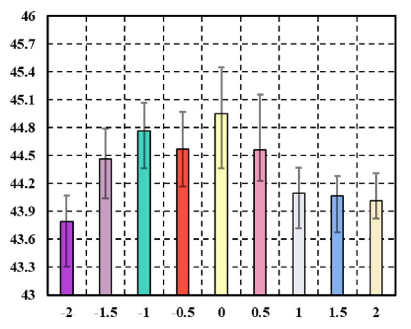
(d) CIFAR-100-LT-100.

Figure 4: Comparison of top-1 validation accuracy(%) of ResNet-32 on CIFAR-LT when varying $\tau$ in Eq.9 for UniMix. The histogram indicates average results in repeated experiments.

Do minorities really get improved? To observe the amelioration on tail classes, Fig.5 visualizes $\log$-confusion matrices on CIFAR-100-LT-100. In Fig.5(e), our method exhibits satisfactory generalization on the tail. Vanilla ERM model (Fig.5(a)) is a trivial predictor which simplifies tail instances as head labels to minimize the error rate. Feature improvement [12] and loss modification [8, 62] methods do alleviate LT problem to some extent. The misclassification cases (i.e., non-diagonal elements) in Fig.5(b),5(c),5(d) become smaller and more balanced distributed compared with ERM. However, the error cases are still mainly in the upper or lower triangular, indicating the existence of inherent bias between the head and tail. Our method (Fig.5(e)) significantly alleviates such dilemma. The non-diagonal elements are more uniformly distributed throughout the matrix rather than in the corners, showing superiority to erase the bias in LT scenarios. Our method enables effective feature improvement for data-scarce classes and alleviates the prior bias, suggesting our success in regularizing tail remarkably.

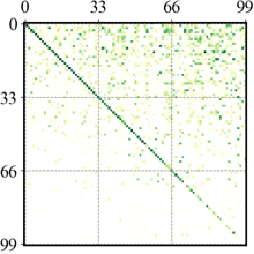
(a) ERM

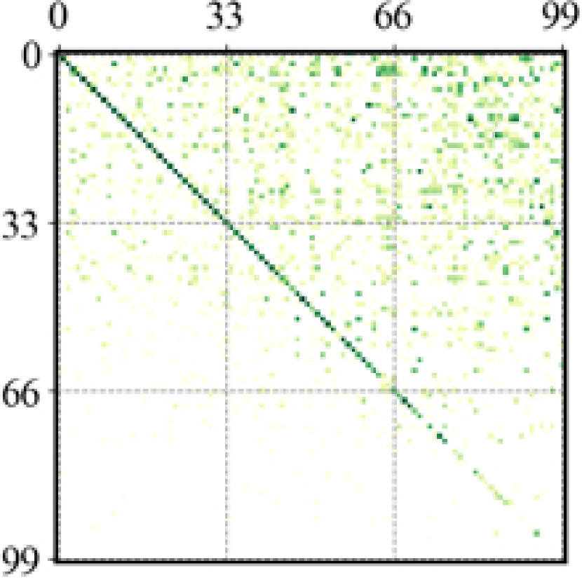
(b) LDAM+DRW [8]

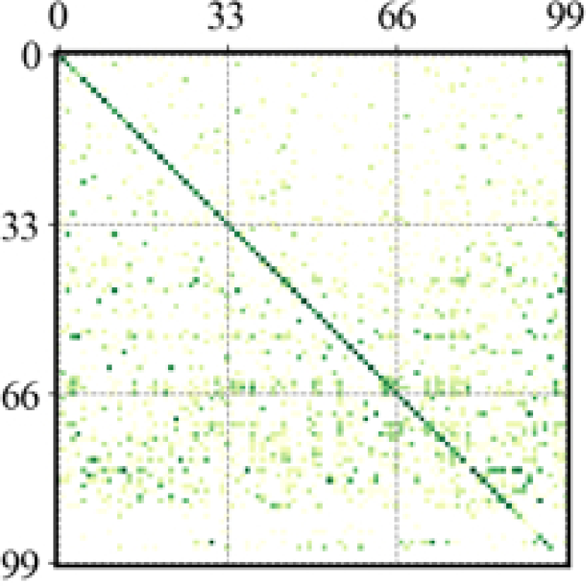
(c) CDT [62]

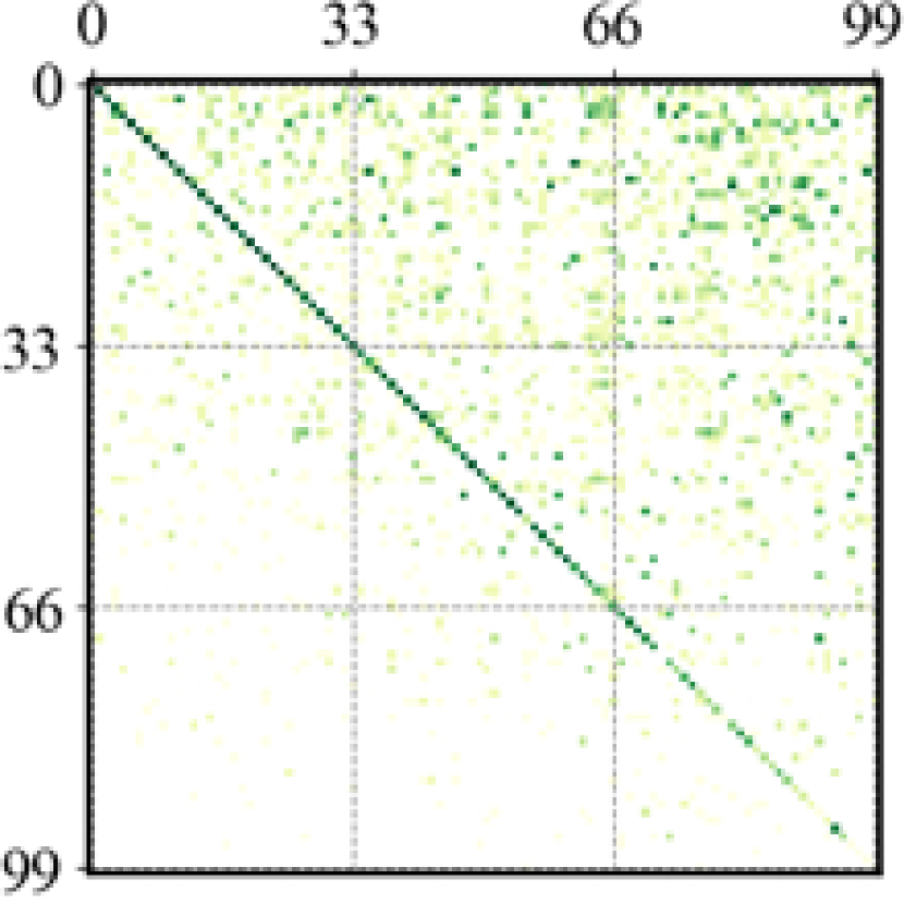
(d) Remix [12]

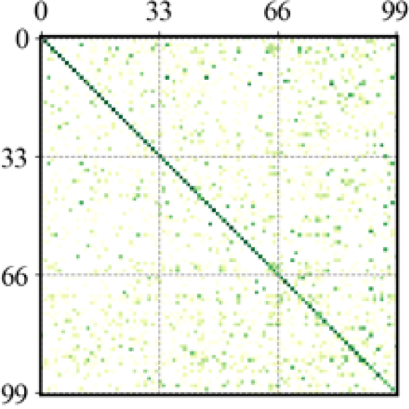
(e) Ours

Figure 5: The $\log$-confusion matrix on CIFAR-100-LT-100 validation dataset. The $x$-axis and $y$-axis indicate the ground truth and predicted labels, respectively. Deeper color indicates larger values.

5 Related work and discussion

Why need calibration? To quantify the predictive uncertainty, calibration [3] is put forward to describe the relevance between predictive score and actual correctness likelihood. A well-calibrated model is more reliable with better interpretability, which probabilities indicate optimal expected costs in Bayesian decision scenarios [46]. Guo et al. [18] firstly provide metric to measure the calibration of CNN and figure out well-performed models are always in lack of calibration, indicating that CNN is sensitive to be overconfidence and lacks robustness. Thulasidasan et al. [58] point out that the effectiveness of mixup in balanced datasets originates from superior calibration modification. Menon et al. [47] further show how to ensure optimal classification calibration for a pair-wise loss.

Feature-wise methods. Intuitively, under-sampling the head [20, 6, 22] or over-sampling the tail [11, 6, 48, 54, 7] can improve the inconsistent performance of imbalanced datasets but tend to either weaken the head or over-fitting the tail. Hence, many effective works generate additional samples [13, 67, 36] to compensate the tail classes. BBN [69] uses two branches to extract features from head and tail simultaneously, while c-RT [33] trains feature representation learning and classification stage separately. mixup [64] and its variants [59, 63, 12] are effective and easy-implement feature-wise methods that convexly combine input and label pairs to generate virtual samples. However, naïve mixup manners are deficient in LT scenarios as we discussed in Sec.2. In contrast, our UniMix tackles such a dilemma by constructing class balance-oriented virtual data as describe in Sec.3.1 and shows satisfactory calibration as Fig.1 exhibits.

Loss modification. Numerous experimental and theoretical studies [50, 14, 57, 61] have demonstrated the existence of inherent bias between LT train set and balanced test set in supervised learning. Previous works [30, 31, 34, 14, 41] make networks prefer learning tail samples by additional class-related weight on CE loss. Some works further correct CE according to the gradient generated by different samples [56, 39] or from the perspective of Gaussian distribution and Bayesian estimation [21, 35]. Meta-learning approaches [17, 1, 55, 51, 32] optimize the weights of each class in CE as learnable parameters and achieve remarkable success. Cao et al. [8] theoretically provides the ideal optimal margin for CE from the perspective of VC generalization bound. Compared with Logit Adjustment [47] motivated by balance error rate, our Bayias-compensated CE eliminates bias incured by prior and is consistent with balanced datasets, which ensures classification calibration as well.

6 Conclusion

We systematically analyze the limitations of mainstream feature improvement methods, i.e., mixup and its extensions in the label-imbalanced situation, and propose the UniMix to construct a more class-balanced virtual dataset that significantly improves classification calibration. We further pinpoint an inherent bias induced by the inconstancy of label distribution prior between long-tailed train set and balanced test set. We prove that the standard cross-entropy loss with the proposed Bayias compensated can ensure classification calibration. The combination of UniMix and Bayias achieves state-of-the-art performance and contributes to a better-calibrated model (Fig.1). Further study in Tab.4 shows that the bad calibration methods are counterproductive with each other. However, more in-depth analysis and theoretical guarantees are still required, which we leave for our future work.

Appendix A Missing proofs and derivations of UniMix

A.1 Basic setting

Setting 1

Without loss of generality, we suppose that the long-tailed distribution satisfies some kind exponential distribution with parameter $\lambda$ [14]. The imbalance factor is defined as $\rho=n_{\max}/n_{\min}$, where $n_{\max}$ and $n_{\min}$ represent the number of the most and least samples in the dataset with $C$ classes, respectively. Then the probability of class $Y$ belongs to $y_{i}$ is:

$$\mathds{P}(Y=y_{i})=\left\{\begin{array}[]{lll}\alpha e^{-\lambda y_{i}}&&{y_{i}\in[1,C]}\\ 0&&{others}\end{array}\right.\quad\sim\quad long-tailed\ \ distribution$$ (A.1)

According to the definition of $\rho$, we can directly deduce the relationship between $\rho$ and $\lambda$:

$$\rho =\frac{n_{\max}}{n_{\min}}=\frac{\mathds{P}(Y=y_{i})_{\max}}{\mathds{P}(Y=y_{i})_{\min}}\Rightarrow\frac{\mathds{P}(Y=y_{1})}{\mathds{P}(Y=y_{C})}=\frac{\alpha e^{-\lambda\cdot 1}}{\alpha e^{-\lambda\cdot C}}\quad\Rightarrow\quad\lambda=\frac{\ln\rho}{C-1}$$ (A.2)

Considering the normalization of probability density, we have:

$$\int_{y_{i}\in\mathcal{Y}}{\mathds{P}(Y=y_{i})dy_{i}} =\int_{1}^{C}{\alpha{e^{-\lambda{y_{i}}}}d{y_{i}}}\equiv 1$$ (A.3)

$$\left.\Rightarrow-\frac{\alpha}{\lambda}e^{-\lambda y_{i}}\right|_{1}^{C}\equiv 1\Rightarrow\frac{\alpha}{\lambda}\left({{e^{-\lambda}}-{e^{-\lambda C}}}\right)\equiv 1$$

$$\Rightarrow\alpha=\frac{\lambda}{{{e^{-\lambda}}-{e^{-\lambda C}}}}$$

Hence, we can express the distribution of LT dataset $\mathcal{D}_{train}$, i.e., $\mathds{P}(Y=y_{i})$ represents the probability of class $y_{i}$ in $\mathcal{D}_{train}$, which can be calculated as follows:

$$\mathds{P}(Y=y_{i})=\frac{{\iint_{x_{i}\in\mathcal{X},y_{j}\in\mathcal{Y}}{\mathds{1}(X=x_{i},Y=y_{i})dx_{i}dy_{j}}}}{{\iint_{{x_{i}}\in\mathcal{X},{y_{j}}\in\mathcal{Y}}{\mathds{1}(X={x_{i}},Y={y_{j}})dx_{i}dy_{j}}}}=\frac{\lambda}{e^{-\lambda}-e^{-\lambda C}}{e^{-\lambda y_{i}}},y_{i}\in[1,C]$$ (A.4)

Notice that Eq.A.4 is determined by total class number $C$ and the imbalance factor $\rho$.

A.2 Proof of Corollary 1

Corollary 1

When $\bm{\xi\sim Beta(\alpha,\alpha)},\alpha\in[0,1]$, the newly mixed dataset $\mathcal{D}_{\nu}$ composed of $\xi$-Aug samples $(\widetilde{x}_{i,j},\widetilde{y}_{i,j})$ follows the same long-tailed distribution as the origin dataset $\mathcal{D}_{train}$, where $(x_{i},y_{i})$ and $(x_{j},y_{j})$ are randomly sampled from $\mathcal{D}_{train}$.

$$\mathds{P}_{\textit{mixup}}(Y^{*}={y_{i}}) =\mathds{P}^{2}(Y={y_{i}})+\mathds{P}(Y={y_{i}})\iint_{y_{i}\neq y_{j}}{Beta(\alpha,\alpha)}\mathds{P}(Y={y_{j}})d\xi dy_{j}$$ (A.5)

$$=\frac{\lambda}{e^{-\lambda}-e^{-\lambda C}}{e^{-\lambda y_{i}}},y_{i}\in[1,C]$$

Proof A.1

Follow the Basic Setting 1, when mixing factor $\xi\sim Beta(\alpha,\alpha)$, consider a $\xi$-Aug sample generated by $\widetilde{x}_{i,j}=\xi\cdot x_{i}+(1-\xi)\cdot x_{j}$ and $\widetilde{y}_{i,j}=\xi\cdot y_{i}+(1-\xi)\cdot y_{j}$. The $\xi$-Aug sample $\widetilde{x}_{i,j}$ contributes to class $y_{i}$ when both pair samples $(x_{i},y_{i})$ and $(x_{j},y_{j})$ are in class $y_{i}$ or one of them are in other labels while the mixing factor $\xi$ is in favor of class $y_{i}$.

$$\mathds{P}({\tilde{y}_{i,j}} ={y_{i}})=\mathds{P}({\tilde{y}_{i,j}}={y_{i}})\cdot\mathds{P}({\tilde{y}_{i,j}}={y_{i}}){\mathds{P}_{\xi}}(0\leq\xi\leq 1)$$ (A.6)

$$\quad+\mathds{P}({\tilde{y}_{i,j}}={y_{i}})\cdot\mathds{P}({\tilde{y}_{i,j}}\neq{y_{i}}){\mathds{P}_{\xi}}(\xi\geq 0.5)$$

$$\quad+\mathds{P}({\tilde{y}_{i,j}}\neq{y_{i}})\cdot\mathds{P}({\tilde{y}_{i,j}}={y_{i}}){\mathds{P}_{\xi}}(\xi<0.5)$$

Hence, the distribution of new dataset $D_{\nu}$ is:

$$\mathds{P}_{\textit{mixup}}(Y={y_{i}}) =\mathds{P}(Y={y_{i}})\cdot\mathds{P}(Y={y_{i}})\cdot\int_{0\leq\xi\leq 1}{Beta(\alpha,\alpha)d\xi}$$ (A.7)

$$\quad+\mathds{P}(Y={y_{i}})\cdot\int_{{y_{j}}\neq{y_{i}}}\int_{\xi\geq 0.5}{Beta(\alpha,\alpha)\cdot\mathds{P}(Y={y_{j}})d\xi d{y_{j}}}$$

$$\quad+\int_{{y_{j}}\neq{y_{i}}}\int_{\xi<0.5}{Beta(\alpha,\alpha)\cdot\mathds{P}(Y={y_{j}})d\xi d{y_{j}}}\cdot\mathds{P}(Y={y_{i}})$$

$$=\mathds{P}^{2}(Y={y_{i}})+0.5\cdot\mathds{P}(Y={y_{i}})\cdot(1-\mathds{P}(Y={y_{i}}))$$

$$\quad+0.5\cdot(1-\mathds{P}(Y={y_{i}}))\cdot\mathds{P}(Y={y_{i}})$$

$$=\mathds{P}^{2}(Y={y_{i}})+0.5\cdot\mathds{P}(Y=y_{i})-0.5\cdot\mathds{P}^{2}(Y=y_{i})$$

$$\quad+0.5\cdot\mathds{P}(Y=y_{i})-0.5\cdot\mathds{P}^{2}(Y=y_{i})$$

$$=\mathds{P}(Y={y_{i}})=\frac{\lambda}{e^{-\lambda}-e^{-\lambda C}}{e^{-\lambda y_{i}}}$$

According to Eq.A.4 and Eq.A.7, the $\xi$-Aug samples in mixed dataset $\mathcal{D}_{\nu}$ generated by mixup follow the same distribution of the original long-tailed one. Therefore, the head gets more regulation than the tail. One the one hand, the classification performance will be promoted. On the other hand, however, the performance gap between the head and tail still exists.

A.3 Proof of Corollary 2

Corollary 2

When $\bm{\xi_{i,j}^{*}\sim\mathscr{U}(\pi_{y_{i}},\pi_{y_{j}},\alpha,\alpha)},\alpha\in[0,1]$, the newly mixed dataset $\mathcal{D}_{\nu}$ composed of $\xi$-Aug samples $(\widetilde{x}_{i,j},\widetilde{y}_{i,j})$ follows a middle-majority distribution, where $(x_{i},y_{i})$ and $(x_{j},y_{j})$ are both randomly sampled from $\mathcal{D}_{train}$.

$$\mathds{P}_{\textit{mixup}}^{*}(Y^{*}={y_{i}}) =\mathds{P}(Y={y_{i}})\int_{y_{j}<{y_{i}}}{\mathds{1}\left(\int{\xi^{*}_{i,j}\mathscr{U}(\pi_{i},\pi_{j},\alpha,\alpha)d\xi^{*}_{i,j}\geq 0.5}\right)\mathds{P}(Y={y_{j}})dy_{j}}$$ (A.8)

$$=\frac{\lambda}{{{{\left({{e^{-\lambda}}-{e^{-C\lambda}}}\right)}^{2}}}}\left({{e^{-\lambda\left({{y_{i}}+1}\right)}}-{e^{-2\lambda{y_{i}}}}}\right),y_{i}\in[1,C]$$

Proof A.2

Follow the settings of Proof A.2 and Eq.6, we can get the following relationship of the label $y_{i}$ and $y_{j}$ with UniMix Factor $\xi_{i,j}^{*}$. It easy to know $\pi_{y_{i}}\leq\pi_{y_{j}}$ if the index $i\geq j$ for the reason that class $y_{j}$ occupies more instances than class $y_{i}$ in long-tailed distribution described as Eq.A.4. Under this circumstances, if consider UniMix Factor $\xi_{i,j}^{*}$ as a constant intuitively, we can deduce that $\xi_{i,j}=\pi_{y_{j}}/(\pi_{y_{i}}+\pi_{y_{j}})\geq 0.5$, i.e.,

$$i\geq j\quad\Rightarrow\quad\pi_{y_{i}}\leq\pi_{y_{j}}\quad\Rightarrow\quad\xi_{i,j}=\frac{\pi_{y_{i}}}{\pi_{y_{i}}+\pi_{y_{j}}}\geq 0.5$$ (A.9)

To improve the robustness and generalization, we consider $\xi_{i,j}^{*}\sim\mathscr{U}(\pi_{y_{i}},\pi_{y_{j}},\alpha,\alpha)$, which extends $\xi_{i,j}^{*}$ to $\pi_{y_{j}}/(\pi_{y_{i}}+\pi_{y_{j}})$ and its vicinity. Hence we can generalize Eq.A.9 to:

$$y_{i}\geq y_{j}\quad\Rightarrow\quad\pi_{y_{i}}\leq\pi_{y_{j}}\quad\Rightarrow\quad\xi_{i,j}\geq 0.5\Rightarrow\int{\xi^{*}_{i,j}\mathscr{U}(\pi_{i},\pi_{j},\alpha,\alpha)d\xi^{*}_{i,j}\geq 0.5}$$ (A.10)

Given any $i,j\in[1,C]$, the $\widetilde{x}_{i,j}$ will tend to be a $\xi$-Aug sample of the class $y_{i}$ if $i\geq j$ for the tail-favored mixing factor. In other words, $\widetilde{x}_{i,j}$ will be a $\xi$-Aug sample for class $y_{i}$ with the mean of $\xi_{i,j}^{*}$ to be $\pi_{y_{j}}/(\pi_{y_{i}}+\pi_{y_{j}})$. Hence, the probability that $\widetilde{x}_{i,j}$ belongs to class $y_{i}$ is:

$$\mathds{P}^{*}_{\textit{mixup}}(Y=y_{i}) =\mathds{P}(Y=y_{i})\cdot\mathds{1}\left({\int{\xi_{i,j}^{*}\mathscr{U}({\pi_{i}},{\pi_{j}},\alpha,\alpha)d\xi_{i,j}^{*}\geq 0.5}}\right)\cdot\mathds{P}(Y<{y_{i}})$$ (A.11)

$$=\mathds{P}(Y={y_{i}})\int_{y_{j}<{y_{i}}}{\mathds{1}\left(\int{\xi^{*}_{i,j}\mathscr{U}(\pi_{i},\pi_{j},\alpha,\alpha)d\xi^{*}_{i,j}\geq 0.5}\right)\mathds{P}(Y={y_{j}})dy_{j}}$$

$$=\mathds{P}(Y={y_{i}})\cdot\int_{1}^{y_{i}}{\mathds{P}(Y={y_{j}})d{y_{j}}}$$

$$=\frac{\lambda}{{{e^{-\lambda}}-{e^{-\lambda C}}}}{e^{-\lambda{y_{i}}}}\cdot\int_{1}^{y_{i}}{\frac{\lambda}{{{e^{-\lambda}}-{e^{-\lambda C}}}}{e^{-\lambda{y_{j}}}}d{y_{j}}}$$

$$=\frac{\lambda}{{{e^{-\lambda}}-{e^{-\lambda C}}}}{e^{-\lambda{y_{i}}}}\cdot\left.{-\frac{{\frac{\lambda}{{{e^{-\lambda}}-{e^{-\lambda C}}}}}}{\lambda}{e^{-\lambda{y_{j}}}}}\right|_{1}^{y_{i}}$$

$$=\frac{\lambda}{{{{\left({{e^{-\lambda}}-{e^{-C\lambda}}}\right)}^{2}}}}\left({{e^{-\lambda({y_{i}}+1)}}-{e^{-2\lambda{y_{i}}}}}\right)$$

According to Eq.A.11, it’s easy to find a derivative zero point in range [1,C]. Hence, the newly distributed dataset $\mathcal{D}_{\nu}$ generated by mixup with UniMix Factor $\xi^{*}_{i,j}$ follows a middle-majority distribution that most data concentrates on middle classes.

A.4 Proof of Corollary 3

Corollary 3

When $\bm{\xi_{i,j}^{*}\sim\mathscr{U}(\pi_{y_{i}},\pi_{y_{j}},\alpha,\alpha)},\alpha\in[0,1]$, the newly mixed dataset $\mathcal{D}_{\nu}$ composed of $\xi$-Aug samples $(\widetilde{x}_{i,j},\widetilde{y}_{i,j})$ follows a tail-majority distribution, where $(x_{i},y_{i})$ is randomly and $(x_{j},y_{j})$ is inversely sampled from $\mathcal{D}_{train}$, respectively.

$${\mathds{P}_{UniMix}}({Y^{*}}={y_{i}}) =\mathds{P}(Y={y_{i}})\int_{y_{j}<{y_{i}}}{\mathds{1}\left(\int{\xi^{*}_{i,j}\mathscr{U}(\pi_{i},\pi_{j},\alpha,\alpha)d\xi^{*}_{i,j}\geq 0.5}\right)\mathds{P}_{inv}(Y=y_{j})dy_{j}}$$ (A.12)

$$=\frac{\lambda}{{\left({{e^{-\lambda}}-{e^{-C\lambda}}}\right)\left({{e^{-C\tau\lambda}}-{e^{-\tau\lambda}}}\right)}}\left({{e^{-\lambda{y_{i}}\left({\tau+1}\right)}}-{e^{-\lambda\left({\tau+{y_{i}}}\right)}}}\right),y_{i}\in[1,C]$$

Proof A.3

Follow the Basic Setting of Proof.1, suppose $(x_{i},y_{i})$ is randomly sampled from $\mathcal{D}_{train}$, while $(x_{j},y_{j})$ is inversely sampled from $\mathcal{D}_{train}$ related to $\tau$. i.e., the probability of $\mathds{P}(Y=y_{i})$ is:

$$\mathds{P}(Y=y_{i})=\frac{\lambda}{{{e^{-\lambda}}-{e^{-\lambda C}}}}{e^{-\lambda{y_{i}}}}$$ (A.13)

The probability of UniMix Sampler that the sampled class $Y$ belongs to $y_{i}$ is $\mathds{P}_{inv}(Y=y_{j})$:

$${\mathds{P}_{inv}}(Y={y_{j}}) =\frac{{{\mathds{P}^{\tau}}(Y={y_{j}})}}{{\int_{{y_{k}}\in\mathcal{Y}}{{\mathds{P}^{\tau}}(Y={y_{k}})d{y_{k}}}}}$$ (A.14)

$$=\frac{{{{\left({\frac{\lambda}{{{e^{-\lambda}}-{e^{-\lambda C}}}}{e^{-\lambda{y_{j}}}}}\right)}^{\tau}}}}{{\int_{{y_{k}}\in\mathcal{Y}}{{{\left({\frac{\lambda}{{{e^{-\lambda}}-{e^{-\lambda C}}}}{e^{-\lambda{y_{k}}}}}\right)}^{\tau}}d{y_{k}}}}}$$

$$=\frac{{{e^{-\lambda\tau{y_{j}}}}}}{{\int_{1}^{C}{{e^{-\lambda\tau{y_{k}}}}d{y_{k}}}}}=\frac{{\lambda\tau{e^{-\lambda\tau{y_{j}}}}}}{{{e^{-\lambda\tau}}-{e^{-\lambda\tau C}}}}$$

Follow the same proof as Proof.A.3, the probability that $\widetilde{x}_{i,j}$ belongs to class $y_{i}$ is:

$$\mathds{P}_{\textit{UniMix}}(Y=y_{i}) =\mathds{P}(Y=y_{i})\cdot\mathds{1}\left({\int{\xi_{i,j}^{*}\mathscr{U}({\pi_{i}},{\pi_{j}},\alpha,\alpha)d\xi_{i,j}^{*}\geq 0.5}}\right)\cdot\mathds{P}_{inv}(Y<{y_{i}})$$ (A.15)

$$=\mathds{P}(Y={y_{i}})\int_{y_{j}<{y_{i}}}{\mathds{1}\left(\int{\xi^{*}_{i,j}\mathscr{U}(\pi_{i},\pi_{j},\alpha,\alpha)d\xi^{*}_{i,j}\geq 0.5}\right)\mathds{P}_{inv}(Y={y_{j}})dy_{j}}$$

$$=\mathds{P}(Y={y_{i}})\cdot\int_{1}^{y_{i}}{\mathds{P}_{inv}(Y={y_{j}})d{y_{j}}}$$

$$=\frac{\lambda}{{{e^{-\lambda}}-{e^{-\lambda C}}}}{e^{-\lambda{y_{i}}}}\cdot\int_{1}^{y_{i}}{\frac{{\lambda\tau{e^{-\lambda\tau{y_{j}}}}}}{{{e^{-\lambda\tau}}-{e^{-\lambda\tau C}}}}d{y_{j}}}$$

$$=\frac{\lambda}{{{e^{-\lambda}}-{e^{-\lambda C}}}}{e^{-\lambda{y_{i}}}}\cdot\left.{\frac{{-{e^{-\lambda\tau{y_{j}}}}}}{{{e^{-\lambda\tau}}-{e^{-\lambda\tau C}}}}}\right|_{1}^{y_{i}}$$

$$=\frac{\lambda}{{\left({{e^{-\lambda}}-{e^{-C\lambda}}}\right)\left({{e^{-C\tau\lambda}}-{e^{-\tau\lambda}}}\right)}}\left({{e^{-\lambda{y_{i}}\left({\tau+1}\right)}}-{e^{-\lambda\left({\tau+{y_{i}}}\right)}}}\right)$$

According to Eq.A.15, $\mathds{P}_{\textit{UniMix}}(Y=y_{i})$ is a gently increasing function in range [1,C]. Hence, the newly mixed dataset $\mathcal{D}_{\nu}$ generated by UniMix follows a tail-majority distribution that adequate data concentrates on tail classes.

A.5 More visualization of Corollary 1,2,3

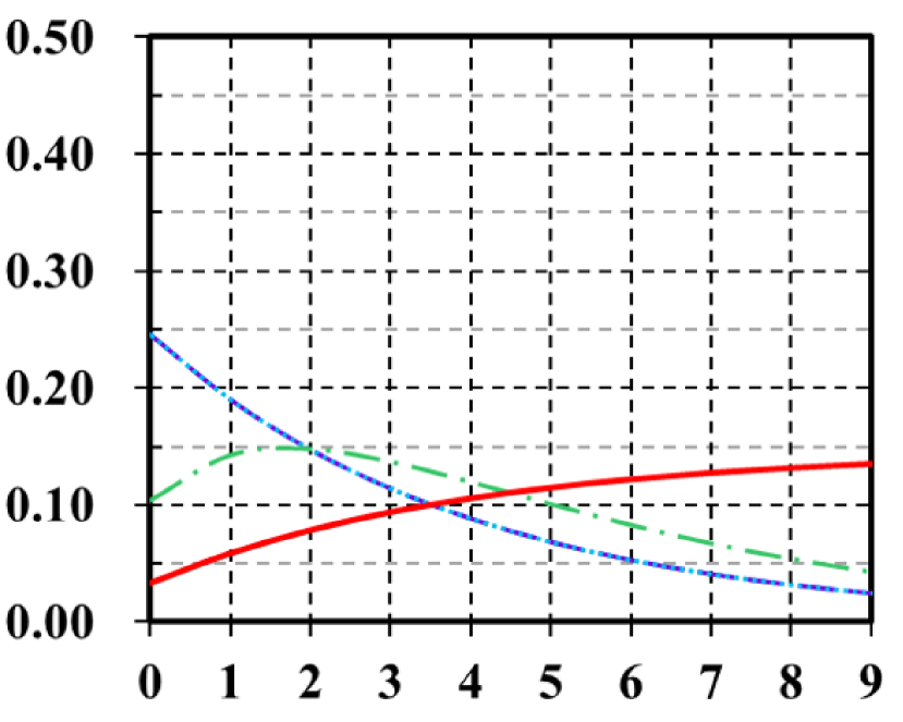
(a) $C=10,\rho=10$

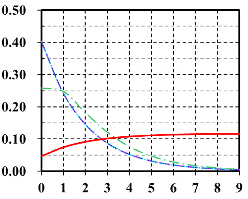
(b) $C=10,\rho=100$

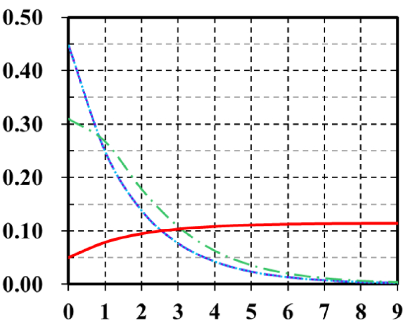
(c) $C=10,\rho=200$

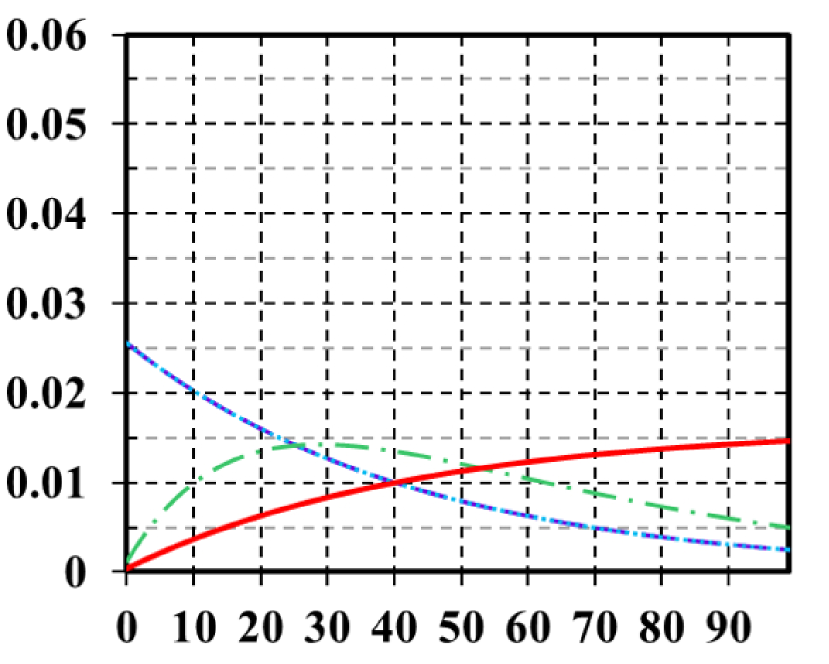
(d) $C=100,\rho=10$

(e) $C=100,\rho=100$

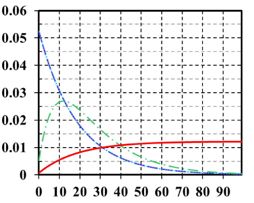
(f) $C=100,\rho=200$

Figure A1: Additional visualized comparisons of $\xi$-Aug samples distribution in Corollary 1,2,3. $x$-axis: class indices. $y$-axis: probability of each class. mixup (blue) exhibits the same LT distribution as origin (purple). UniMix Factor (green) alleviates such situation and the full pipeline ($\tau$=$-1$) constructs a more uniform distribution of $\xi$-Aug (red), which contributes to a well-calibrated model.

We present additional visualized distribution of $\xi$-Aug samples with different sample strategies for comprehensive comparisons, including $\rho\in\{10,100,200\}$ and $C\in\{10,100\}$. As illustrated in Fig.A1, when the class number $C$ and imbalance factor $\rho$ get larger, the limitations of mixup in LT scenarios gradually appear. The VRM dataset $\mathcal{D}_{\nu}$ generated by mixup with naïve mixing factor and random sampler will make $\mathcal{D}_{\nu}$ following the same LT distribution. The newly mixed pseudo data by mixup follows the head-majority distribution. It has limited contribution for the tail class’ feature learning and regulation, which is the reason for its poor calibration.

In contrast, the proposed UniMix Factor $\xi^{*}_{i,j}$ significantly promotes such situation and improves tail class’s feature learning by the preference on the relatively fewer classes of the two samples in a pair. Because of the random sampler, the samples are still mainly from the head, and the newly mixed dataset will follows a middle-majority distribution. Most data concentrates on the middle of classes as green line shows. As $C$ and $\rho$ get larger, the middle distribution will get close to the head. Thanks to the UniMix Sampler that inversely draws data from $\mathcal{D}_{train}$, the $D_{\nu}$ is mainly composed of the head-tail pairs that contribute to the feature learning for the tail when integrated with UniMix Factor. As a result, $D_{\nu}$ follows the tail-majority distribution that improves the generalization on the tail. Specifically, when $C$ and $\rho$ get larger, the distribution of $D_{\nu}$ generated by UniMix still maintains satisfactory tail-majority distribution.

Appendix B Missing Proofs and derivations of Bayias

B.1 Proof of Bayias

Theorem B.1

For classification, let $\psi(x;\theta,W,b)$ be a hypothesis class of neural networks of input $X=x$, the classification with Softmax should contain the influence of prior, i.e., the predicted label during training should be:

$$\hat{y}=\mathop{\arg\max}_{y_{i}\in\mathcal{Y}}\frac{{{e^{\psi{{(x;\theta,W,b)}_{{y_{i}}}}+\bm{\log(\pi_{y_{i}})+\log(C)}}}}}{{\sum\nolimits_{{y_{j}}\in\mathcal{Y}}{{e^{\psi{{(x;\theta,W,b)}_{{y_{j}}}}+\bm{\log(\pi_{y_{j}})+\log(C)}}}}}}$$ (B.1)

Proof B.1

Generally, a classifier can be modeled as:

$$\hat{y}=\mathop{\arg\max}_{y_{i}\in\mathcal{Y}}\frac{e^{\sum\nolimits_{{d_{i}}\in D}[{{{({W^{T}})_{{y_{i}}}^{({d_{i}})}\mathcal{F}{{(x;\theta)}^{(d_{i})}}]+{b_{{y_{i}}}}}}}}}{{\sum\nolimits_{{y_{j}}\in\mathcal{Y}}e^{\sum\nolimits_{{d_{i}}\in D}[{{{({W^{T}})_{{y_{j}}}^{({d_{i}})}\mathcal{F}{{(x;\theta)}^{(d_{i})}}]+{b_{{y_{j}}}}}}}}}}\triangleq\mathop{\arg\max}_{y_{i}\in\mathcal{Y}}\frac{{{e^{\psi{{(x;\theta,W,b)}_{{y_{i}}}}}}}}{{\sum\nolimits_{{y_{j}}\in\mathcal{Y}}{{e^{\psi{{(x;\theta,W,b)}_{{y_{j}}}}}}}}}$$ (B.2)

where $\hat{y}$ indicates the predicted label and $\mathcal{F}(x;\theta)\in\mathds{R}^{D\times 1}$ is the $D$-dimension feature extracted by the backbone with parameter $\theta$. $W\in\mathds{R}^{D\times C}$ represents the parameter matrix of the classifier. The model attempts to get the maximum $\hat{y}$ given $x$, i.e., to maximize the posterior, satisfying the following relationship between the prior and likelihood according to the Bayesian theorem:

$$\hat{y} =\mathop{\arg\max}_{y_{i}\in\mathcal{Y}}{\mathds{P}}(Y={y_{i}}|X={x})$$ (B.3)

$$=\mathop{\arg\max}_{y_{i}\in\mathcal{Y}}\frac{{{\mathds{P}}(X={x}|Y={y_{i}})\cdot{\mathds{P}}(Y={y_{i}})}}{{\sum\nolimits_{k}{\mathds{P}(Y={y_{k}})\prod\nolimits_{j}{\mathds{P}({X^{(j)}}={x^{(j)}}|Y={y_{k}})}}}}$$

$$\propto\mathop{\arg\max}_{y_{i}\in\mathcal{Y}}\mathds{P}(X=x|Y=y_{i})\cdot\mathds{P}(Y=y_{i})$$

where $\sum\nolimits_{k}{\mathds{P}(Y={y_{k}})\prod\nolimits_{j}{\mathds{P}({X^{(j)}}={x^{(j)}}|Y={y_{k}})}}$ is the normalized evidence factor. $\mathds{P}(Y=y_{i})$ is the prior probability estimated by the instance proportion of each category in the dataset. To maximize posterior, we need to get the $\mathds{P}(X|Y)$ in an ERM supervised training manner. However, in LT scenarios, the likelihood is consistent in the train and test set, but the prior is different. Hence, we derive the posterior on train and test set separately:

$$\left\{\begin{aligned} &\hat{y}\propto\mathop{\arg\max}_{y_{i}\in\mathcal{Y}}\mathds{P}(X=x|Y=y_{i})\cdot\mathds{P}_{train}(Y=y_{i})\\ &\hat{y}^{\prime}\propto\mathop{\arg\max}_{y_{i}\in\mathcal{Y}}\mathds{P}(X=x^{\prime}|Y^{\prime}=y_{i})\cdot\mathds{P}^{\prime}_{test}(Y^{\prime}=y_{i})\end{aligned}\right.$$ (B.4)

where $\hat{y},\hat{y}^{\prime}$ represent the prediction results for the train and test set, respectively. The model $\psi(x;\theta,W,b)$ is just the likelihood estimation $\mathds{P}(X=x|Y=y_{i})$ of the train set. To obtain the posterior probability $y^{\prime}=\mathop{\arg\max}_{y_{i}\in\mathcal{Y}}{\mathds{P}^{\prime}(Y=y_{i}|X=x^{\prime})}$ for inference, one should consider unifying the optimization direction on the train set and test set:

$$\mathds{P}_{test}(Y=y_{i}|X=x^{\prime}) \propto\frac{\mathds{P}_{train}(Y=y_{i}|X=x)}{\mathds{P}_{train}(Y=y_{i})}\cdot\mathds{P}_{test}(Y^{\prime}=y_{i})=\frac{\mathds{P}_{train}(Y=y_{i}|X=x)}{C\cdot\pi_{y_{i}}}$$ (B.5)

For the difference of label prior, the learned parameters of the model will also yield class-level bias. Hence, the actual optimization direction is not described as Eq.B.2 because the bias incurred by prior should be compensated at first.

$$\hat{\theta},\hat{W},\hat{b}\triangleq\Theta =\mathop{\arg\min}_{\Theta}\sum\nolimits_{\begin{subarray}{c}{x_{i}\in\mathcal{X}^{\prime}\land y_{i}\in\mathcal{Y}}\end{subarray}}\mathds{1}\left({y_{i}}\neq\mathop{\arg\max}_{y_{j}\in\mathcal{Y}}({\mathds{P}_{test}(Y={y_{j}}|X={x_{i}})}\right)$$ (B.6)

$$\Leftrightarrow\mathop{\arg\min}_{\Theta}\sum\nolimits_{\begin{subarray}{c}{x_{i}\in\mathcal{X}\land y_{i}\in\mathcal{Y}}\end{subarray}}\mathds{1}\left({y_{i}}\neq\mathop{\arg\max}_{y_{j}\in\mathcal{Y}}\frac{\mathds{P}_{train}(Y=y_{j}|X=x_{i})}{C\cdot\pi_{y_{j}}}\right)$$

$$=\mathop{\arg\min}_{\Theta}\sum\nolimits_{\begin{subarray}{c}{x_{i}\in\mathcal{X}\land y_{i}\in\mathcal{Y}}\end{subarray}}\mathds{1}\left({y_{i}}\neq\mathop{\arg\max}_{y_{j}\in\mathcal{Y}}\frac{e^{\psi(x_{i};\theta,W,b)_{y_{j}}-\bm{\log C-\log(\pi_{y_{j}})}}}{{\sum\nolimits_{{y_{k}}\in\mathcal{Y}}{e^{\psi{{(x_{i};\theta,W,b)}_{{y_{k}}}}}}}}\right)$$

$$\Leftrightarrow\mathop{\arg\min}_{\Theta}\sum\nolimits_{\begin{subarray}{c}{x_{i}\in\mathcal{X}\land y_{i}\in\mathcal{Y}}\end{subarray}}\mathds{1}\left({y_{i}}\neq\mathop{\arg\max}_{y_{j}\in\mathcal{Y}}\frac{e^{\psi(x_{i};\theta,W,b)_{y_{j}}-\bm{\log(\pi_{y_{j}})-\log C}}}{{\sum\nolimits_{{y_{k}}\in\mathcal{Y}}{e^{\psi{{(x_{i};\theta,W,b)}_{{y_{k}}}}-\bm{\log(\pi_{y_{k}})-\log C}}}}}\right)$$

To correct the bias for inferring, the offset term that the model in LT datasets needs to compensate is:

$$\mathscr{B}_{y}=log(\pi_{y})+log(C)$$ (B.7)

B.2 Proof of classification calibration

Theorem B.2

$\mathscr{B}_{y}$-compensated cross-entropy loss in Eq.B.8 ensures classification calibration.

$$\mathcal{L}_{\mathscr{B}}\left({y_{i},\psi(x;\Theta)}\right)=-\log\frac{{{e^{\psi{{(x;\Theta)}_{{y_{i}}}}+\log\left({{\pi_{{y_{i}}}}}\right)+\log\left(C\right)}}}}{{\sum\nolimits_{{y_{k}}\in\mathcal{Y}}{{e^{\psi{{(x;\Theta)}_{y_{j}}}+\log\left({{\pi_{{y_{k}}}}}\right)+\log\left(C\right)}}}}}$$ (B.8)

Classification calibration [18, 58] represents the predicted winning Softmax scores indicate the actual likelihood of a correct prediction. The miscalibrated models tend to be overconfident which results in that the minimiser of the expected loss (equally, the empirical risk in the infinite sample limit) can not lead to a minimal classification error. Previous work [47] has introduced a theory to measure the calibration of a pair-wise loss:

Lemma B.1

Pairwise loss $\mathcal{L}(y_{i},\psi(x;\Theta))=\alpha_{y_{i}}\cdot\log\left[1+\sum_{y_{k}\neq y_{i}}e^{\Delta_{y_{i}y_{k}}}\cdot e^{(\psi(x;\Theta)_{y_{i}}-\psi(x,\Theta)_{y_{k}})}\right]$ ensures classification calibration if for any $\delta\in\mathds{R}_{+}^{C}$:

$$\alpha_{y_{i}}=\delta_{y_{i}}/\pi_{y_{i}}\ \ \ \ \Delta{y_{i}y_{k}}=\log(\delta_{y_{k}}/\delta_{y_{i}})$$ (B.9)

Proof B.2

To begin, we rewritten the Bayias-compensated cross-entropy loss into the following equation:

$${\mathcal{L}_{\mathscr{B}}}\left({y_{i},\psi(x;\Theta)}\right) =-\log\frac{{{e^{\psi{{(x;\Theta)}_{{y_{i}}}}+\log\left({{\pi_{{y_{i}}}}}\right)+\log\left(C\right)}}}}{{\sum\nolimits_{{y_{k}}\in\mathcal{Y}}{{e^{\psi{{(x;\Theta)}_{y_{j}}}+\log\left({{\pi_{{y_{k}}}}}\right)+\log\left(C\right)}}}}}$$ (B.10)

$$\Leftrightarrow\log\frac{{\sum\nolimits_{{y_{k}}\in\mathcal{Y}}{{e^{\psi{{(x;\Theta)}_{y_{k}}}+\log\left({{\pi_{{y_{k}}}}}\right)+\log\left(C\right)}}}}}{{{e^{\psi{{(x;\Theta)}_{{y_{i}}}}+\log\left({{\pi_{{y_{i}}}}}\right)+\log\left(C\right)}}}}$$

$$=\log\left[{1+\frac{{\sum\nolimits_{{y_{k}}\neq{y_{i}}}{{e^{\psi{{(x;\Theta)}_{{y_{k}}}}+\log\left({{\pi_{{y_{k}}}}}\right)+\log\left(C\right)}}}}}{{{e^{\psi{{({x};\Theta)}_{{y_{i}}}}+\log\left({{\pi_{{y_{i}}}}}\right)+\log\left(C\right)}}}}}\right]$$

$$=\log\left[{1+\sum\nolimits_{{y_{k}}\neq{y_{i}}}{\frac{{{e^{\psi{{(x;\Theta)}_{{y_{k}}}}+\log\left({{\pi_{{y_{k}}}}}\right)+\log\left(C\right)}}}}{{{e^{\psi{{({x};\Theta)}_{{y_{i}}}}+\log\left({{\pi_{{y_{i}}}}}\right)+\log\left(C\right)}}}}}}\right]$$

$$=\log\left[{1+\sum\nolimits_{{y_{k}}\neq{y_{i}}}{\frac{{{e^{\log\left({{\pi_{{y_{k}}}}}\right)+\log\left(C\right)}}\cdot{e^{\psi{{(x;\Theta)}_{{y_{k}}}}}}}}{{{e^{\log\left({{\pi_{{y_{i}}}}}\right)+\log\left(C\right)}}\cdot{e^{\psi{{({x};\Theta)}_{{y_{i}}}}}}}}}}\right]$$

$$=\log\left[{1+\sum\nolimits_{{y_{k}}\neq{y_{i}}}{{e^{\mathscr{B}_{y_{k}}-\mathscr{B}_{y_{i}}}}\cdot{e^{\psi{{(x;\Theta)}_{{y_{k}}}}-\psi{{({x};\Theta)}_{{y_{i}}}}}}}}\right]$$

Compare Eq.B.10 with LemmaB.1, observed that when $\delta_{y}=\pi_{y}$.

$$\left\{\begin{array}[]{lr}\alpha_{y_{i}}=\delta_{y_{i}}/\pi_{y_{i}}=\pi_{y_{i}}/\pi_{y_{i}}=1\\ \begin{aligned} \Delta_{y_{i}y_{k}}&=\mathscr{B}_{y_{k}}-\mathscr{B}_{y_{i}}\\ &=[log(\pi_{y_{k}})+log(C)]-[log(\pi_{y_{i}})+log(C)]\\ &=log(\pi_{y_{k}})-log(\pi_{y_{i}})=log(\pi_{y_{k}}/\pi_{y_{i}})\end{aligned}\end{array}\right.$$ (B.11)

According to LemmaB.1, we immediately deduce that Bayias-compensated cross-entropy loss ensures classification calibration.

B.3 Comparisons with other losses

Previous work [34, 14, 56, 62, 8, 47] adjusts the logits weight or margin on standard Softmax cross-entropy (CE) loss to tackle the long-tailed datasets. We summarize the loss modification methods reported in Tab.1 and discuss the difference between theirs and ours here.

Weight-wise losses.

Focal loss [41] is proposed to balance the positive/negative samples during object detection and extends for classification by assigning low weight loss for easy samples. It re-wights the loss with a factor $(1-p_{y_{i}})^{\gamma}$ on standard cross-entropy loss, where $p_{y_{i}}$ is the prediction probability of class $y_{i}$:

$$\mathcal{L}_{Focal}=-(1-p_{y_{i}})^{\gamma}\log\frac{e^{\psi(x;\Theta)_{y_{i}}}}{\sum\nolimits_{{y_{k}}\in\mathcal{Y}}{{e^{\psi{(x;\Theta)}_{y_{k}}}}}}$$ (B.12)

CB loss is proposed by Cui et al. [14] with the effective number. It adopts a coefficient $(1-\beta)/(1-\beta^{n_{y_{i}}})$ for standard cross-entropy loss:

$$\mathcal{L}_{CB}=-\frac{1-\beta}{1-\beta^{n_{y_{i}}}}\log\frac{e^{\psi(x;\Theta)_{y_{i}}}}{\sum\nolimits_{{y_{k}}\in\mathcal{Y}}{{e^{\psi{(x;\Theta)}_{y_{k}}}}}}$$ (B.13)

CDT loss [62] re-weights each Softmax logit with a temperature scale factor $a_{y_{i}}=(\frac{n_{max}}{n_{y_{i}}})^{\gamma}$. It artificially reduces the decision values for head classes:

$$\mathcal{L}_{CDT}=-\log\frac{e^{\psi(x;\Theta)_{y_{i}}/(\frac{n_{max}}{n_{y_{i}}})^{\gamma}}}{\sum\nolimits_{{y_{k}}\in\mathcal{Y}}{{e^{\psi{(x;\Theta)}_{y_{k}}/(\frac{n_{max}}{n_{y_{k}}})^{\gamma}}}}}$$ (B.14)

All above re-weight methods are proven effective empirically, more or less. However, such approaches will confront the coverage dilemma when the train data gets highly imbalanced. The weights related to instances number may be large in this situation and result in unstable gradients that deteriorate head classes’ performance gain. They are also sensitive to hyper-parameters, which makes it hard to adopt in varied datasets.

Margin-wise losses.

Previous work in Deep Metrics Learning [44, 15, 60, 43] attempts to obtain better inter-class and intra-class distance from the margin perspective. Cao et al. [8] analyze the optimal margin between two different classes via generalization error bounds in the long tail visual recognition. They propose the LDAM loss to encourage the tail classes to enjoy larger margins. In detail, a label-aware margin $C/n_{y_{i}}^{1/4}$ is added to the groud truth logit where $C$ is an independent constant:

$$\mathcal{L}_{LDAM}=-\log\frac{e^{\psi(x;\Theta)_{y_{i}}-C/n_{y_{i}}^{1/4}}}{e^{\psi(x;\Theta)_{y_{i}}-C/n_{y_{i}}^{1/4}}+\sum_{{y_{k}}\neq{y_{i}}}{{e^{\psi{(x;\Theta)}_{y_{k}}}}}}$$ (B.15)

Logit Adjustment [47] loss is proposed to overcome the long-tailed dataset motivated by the balanced error rate. They suppose that the model shows similar performance on each class in the validation dataset. The authors propose a margin $\tau\log(\pi_{y_{i}})$ on standard Softmax cross-entropy loss. Different from the LDAM loss, such margin is added for all logits with label priors $\pi_{y}$:

$$\mathcal{L}_{LA}=-\log\frac{e^{\psi(x;\Theta)_{y_{i}}+\tau\log(\pi_{y_{i}})}}{\sum\nolimits_{{y_{k}}\in\mathcal{Y}}{{e^{\psi{(x;\Theta)}_{y_{k}}+\tau\log(\pi_{y_{k}})}}}}$$ (B.16)

Our Bayias-compensated CE loss is motivated by erasing the difference of label prior in the train set and test set based on the Bayesian theory. The network parameters are only the likelihood estimation, while we need a reliable posterior for unbiased inference. Hence, we compensate the bias incurred by various label prior via adding a margin related to the train set label prior and minus a margin related to the test set label prior:

$$\mathcal{L}_{ours}=-\log\frac{e^{\psi(x;\Theta)_{y_{i}}+\log(\pi_{y_{i}})-\log(1/C)}}{\sum\nolimits_{{y_{k}}\in\mathcal{Y}}{{e^{\psi{(x;\Theta)}_{y_{k}}+\log(\pi_{y_{k}})-\log(1/C)}}}}$$ (B.17)

One may notice that our loss is similar to LA loss with an extra constant margin $-\log(1/C)$ when the $\tau=1$ in LA loss. However, the difference lies in two aspects: 1) the margin $-\log(1/C)$ is a positive value and makes all logits get larger, which makes Softmax operation more distinguishable. 2) Notice our two margins are related to the label prior of the train set and test set. Hence, when the train set is balanced, i.e., $\pi_{y_{i}}=1/C$, the margin will be $\log(1/C)-\log(1/C)\equiv 0$, and our loss coverage to the standard cross-entropy loss. Furthermore, our loss can handle the situation that both train set and test set are imbalanced distribution via directly setting the margin as $\log(\pi_{y_{i}})-\log(\pi^{\prime}_{y_{i}})$, where $\pi_{y_{i}}$ is the label prior in the train set and $\pi^{\prime}_{y_{i}}$ is the label prior in test set correspondingly.

Appendix C Implement detail

We conduct experiments on CIFAR-10-LT [38], CIFAR-100-LT [38], ImageNet-LT [53], and iNaturalist 2018 [28]. We adopt long-tailed version CIFAR datasets which are build by suitably discarding training instances following the Exp files given in [14, 8]. The instance number of each class exponentially decays in train dataset and keeps balanced during validation process. Here, an imbalance factor $\rho$ is define as $n_{max}/n_{min}$ to measure how imbalanced the dataset is. ImageNet-LT is the LT version of ImageNet. It samples instances for each class following Pareto distribution which is also long-tailed. iNaturalist 2018 is a real-world dataset with $8,142$ classes and $\rho=500$, which suffers extremely class-imbalanced and fine-grained problems.

C.1 Implement details on CIFAR-LT

ResNet-32 is the backbone on CIFAR-LT. For all CIFAR-10-LT and CIFAR-100-LT, the universal data augmentation strategies [24] are used for training. Specifically, we pad $4$ pixels on each side and crop a $32\times 32$ region. The cropped regions are flipped horizontally with $0.5$ probability and normalized by the mean and standard deviation for each color channel. We train the model via stochastic gradient decent (SGD) with momentum $0.9$ and weight decay of $2\times 10^{-4}$ for all experiments. All models are trained for $200$ epochs setting mini-batch as $128$ with same learning rate [8] for fair comparisons. The learning rate is set as [8]: the initial value is $0.1$ and linear warm up at first $5$ epochs. The learning rate is decayed at the $160^{th}$ and $180^{th}$ epoch by $0.01$. For all mixup [64] and its extension methods [59, 12], we fine-tune the model after $120^{th}$ epoch. The $\alpha$ of Beta distribution is $0.5$ for UniMix and $1.0$ for others.

C.2 Implement details on large-scale datasets

We adopt ResNet-10 & ResNet-50 for ImageNet-LT and ResNet-50 for iNaturalist 2018. For ImageNet-LT, ResNet-10 and ResNet-50 are trained from scratch for $90$ epochs, setting mini-batch as $512$ and $64$, respectively. For iNaturalist 2018, we adopt the vanilla ResNet-50 with mini-batch as $512$ and train for $90$ epochs. With proper data augment strategy [69], the SGD optimizer with momentum $0.9$ and weight decay $1\times 10^{-4}$ optimizes the model with same learning rate for fair comparisons [8, 69, 33]. We set base learning rate as $0.2$ and decay it at the $30^{th}$ and $60^{th}$ epoch by $0.1$, respectively.

Appendix D Additional Experiment Results

We present additional experiments for comprehensive comparisons with previous methods and make a detailed analysis, which can be summarized as follows:

• Visualized top-1 validation error (%) comparisons of previous methods.

• Additional quantity and visualized comparisons of classification calibration.

• Additional visualized comparisons of confusion matrix and $\log$-confusion matrix.

• Additional comparisons on test imbalance scenarios.

• Additional comparisons on state-of-the-art two-stage method.

D.1 Visualized comparisons on CIFAR-10-LT and CIFAR-100-LT

Previous sections have shown the remarkable performance of the proposed UniMix and Bayias. Fig.D1 shows the visualized top-1 validation error rate (%) comparisons on CIFAR-10-LT and CIFAR-100-LT with $\rho\in\{10,50,100,200\}$ for clear and comprehensive comparisons. The histogram indicates the value of each method. The positive error term represents its distance towards the best method, while the negative term indicates the advance towards the worst one.

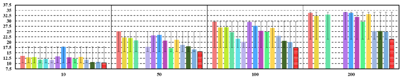
(a) CIFAR-10-LT

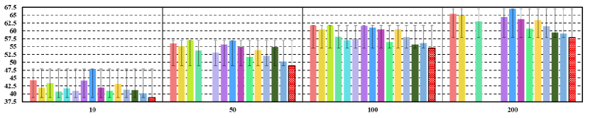
(b) CIFAR-100-LT

Figure D1: Visualized top1 error (%) ($y$-axis) comparisons of CIFAR-10-LT and CIFAR-100-LT on different $\rho$ ($x$-axis) in ResNet-32. The proposed method (red) achieves the lowest error rate compared with other methods. The leading advantage of our method increases consistently as imbalance factor gets larger.

Results in Fig.D1 show that the proposed method outperforms others with lower error rate over all imbalance factors settings. As the dataset gets more skewed and imbalanced, the advantage of our method gradually emerges. On the one hand, the proposed UniMix generates a tail-majority pseudo dataset favoring the tail feature learning, which makes the model achieve better calibration. It is practical to improve the generalization of all classes and avoid potential over-fitting and under-fitting risks. On the other hand, the proposed Bayias overcomes the bias caused by existing prior differences, which improves the model’s performance on the balanced validation dataset. Even in extremely imbalanced scenarios (e.g., CIFAR-100-LT-200), the proposed method still achieves satisfactory performance.

D.2 Additional quantitative and qualitative calibration comparisons

D.2.1 Definition of calibration

Calibration means a model’s predicting probability can estimate the representative of the actual correctness likelihood, which is vital in many real-world decision-making applications [52, 9, 4]. Suppose a dataset contains $N$ samples $\mathcal{D}:=\{(x_{k},y_{k})\}_{k=1}^{N}$, where $x_{i}$ and $y_{i}$ represent the $i^{th}$ sample and its corresponding label, respectively. Let $\hat{p}_{y_{i}}=\mathds{P}(Y=y_{i}|x=x_{i})$ be the confidence of the predicted label, and divide dataset $\mathcal{D}$ into a mini-batch size $m$ with $M=N/m$ in total. The accuracy (acc) and the confidence (cfd) in a mini-batch $\mathcal{B}_{m}$ are:

$$acc(\mathcal{B}_{m})=\frac{1}{m}\sum\nolimits_{i\in{\mathcal{B}_{m}}}{\mathds{1}({\hat{y}_{i}}={y_{i}})}$$ (D.1)

$$cfd(\mathcal{B}_{m})=\frac{1}{m}\sum\nolimits_{i\in{\mathcal{B}_{m}}}{\hat{p}_{y_{i}}}$$

According to Eq.D.1, a perfectly calibrated model will strictly have $acc(\mathcal{B}_{m})\equiv cfd(\mathcal{B}_{m})$ for all $m\in\{1,\cdots,M\}$. Hence, the Expected Calibration Error (ECE) is proposed as a scalar statistic of calibration to quantitatively measure classifiers’ mean distance to the ideal $acc(\mathcal{B}_{m})\equiv cfd(\mathcal{B}_{m})$, which is defined as:

$$ECE=\sum\nolimits_{m=1}^{M}{\frac{{\left|{{\mathcal{B}_{m}}}\right|}}{n}\left|{acc({\mathcal{B}_{m}})-cfd({\mathcal{B}_{m}})}\right|}$$ (D.2)

In addition, reliable confidence measures are essential in high-risk applications. The Maximum Calibration Error (MCE) describes the worst-case deviation between confidence and accuracy, which can be defined as:

$$MCE=\mathop{\max}\limits_{m\in\{1,\cdots,M\}}\left|{acc({\mathcal{B}_{m}})-cfd({\mathcal{B}_{m}})}\right|$$ (D.3)

According to Eq.D.2,D.3, a well-calibrated model should coverage ECE and MCE to $0$, indicating that the prediction score reflects the actual accuracy likelihood. Under this circumstances, the calibrated model will show excellent robustness and generalization, especially in LT scenarios. Although the authors in [18] propose the temperature scaling as a post-hoc method to adjust the classifier, our motivation is to train a calibrated model end to end without loss of accuracy.

Previous work [2] points out that ECE scores suffer from several shortcomings. Hence, additional metrics [49, 2] are proposed to show more robustness, e.g., Adaptivity & Adaptive Calibration Error (ACE), Thresholding & Thresholded Adaptive Calibration Error (TACE), Static Calibration Error (SCE), and Brier Score (BS). The definition of the above metrics are as follows:

TACE disregards all predicted probabilities that are less than a certain threshold $\epsilon$. It adaptively chooses the bin locations to ensure each bin has the same instance numbers and estimates the miscalibration of probabilities across all classes in the prediction while the ECE only chooses the top-1 predicted class. TACE is defined as Eq.D.4:

$$TACE=\frac{1}{CR}\sum\nolimits_{c=1}^{C}\sum\nolimits_{r=1}^{R}|acc(\mathcal{B}_{r},c)-cfd(\mathcal{B}_{r},c)|$$ (D.4)

where $acc(\mathcal{B}_{r},c)$ and $cfd(\mathcal{B}_{r},c)$ are the accuracy and confidence of adaptive calibration range $r$ for class label $c$, respectively. Calibration range $r$ defined by the $\lfloor N/R\rfloor_{th}$ index of the sorted and thresholded predictions, exclude the prediction less than $\epsilon$. If set $\epsilon=0$, TACE converts to ACE.

SCE is a simple extension of ECE to every probability in the multi-class setting. SCE bins predictions separately for each class probability, computes the calibration error within the bin, and averages across bins. SCE is defined as Eq.D.5:

$$SCE=\frac{1}{C}\sum\nolimits_{c=1}^{C}\sum\nolimits_{b=1}^{B}\frac{n_{bc}}{N}|acc(\mathcal{B}_{b},c)-cfd(\mathcal{B}_{b},c)|$$ (D.5)

where $acc(\mathcal{B}_{b},c)$ and $cfd(\mathcal{B}_{b},c)$ are the accuracy and confidence of bin $\mathcal{B}_{b}$ for class label $c$, respectively. $n_{bc}$ is the prediction number in bin $\mathcal{B}_{b}$ for class $c$. $N$ is the total number of test set.

BS [5] has also been known as a metric for the verification of predicted probabilities. Similarly to the log-likelihood, BS penalizes low probabilities assigned to correct predictions and high probabilities assigned to wrong ones, which is defined as Eq.D.6:

$$BS=\frac{1}{NC}\sum\nolimits_{i=1}^{N}\sum\nolimits_{c=1}^{C}\left(\mathds{1}(y_{i}^{*}=c)-\mathds{P}(Y=y_{c}|X=x_{i})\right)^{2}$$ (D.6)

where $N$ represents the total number of test set. $y_{i}^{*}$, $\mathds{P}(Y=y_{c}|X=x_{i})$ represent the ground truth and predicted label, respectively.

D.2.2 Quantitative results of calibration on CIFAR-LT

Besides ECE and MCE results, we additionally provide quantitative metrics results, i.e., ACE, TACE setting threshold $\epsilon=1e-3$, SCE, and BS. The comparisons are illustrated in Tab.D1.

Table D1: Quantitative calibration metric of ResNet-32 on CIFAR-10/100-LT-100 test set. Smaller ACE, TACE, SCE, and BS indicate better calibration results. Either of the proposed methods achieves a well-calibrated model compared with others. The combination of UniMix and Bayias still achieves the best performance.

Dataset	CIFAR-10-LT-100				CIFAR-100-LT-100
Calibration Metric ($\times$ 100)	ACE	TACE	SCE	BS	ACE	TACE	SCE	BS
ERM	5.42	4.66	5.46	53.61	0.831	0.709	0.952	97.05
mixup [64]	4.87	4.20	4.92	49.09	0.751	0.683	0.849	89.26
Remix [12]	3.49	3.32	3.77	44.84	0.740	0.675	0.846	89.33
LDAM+DRW [8]	4.14	2.84	4.43	44.76	0.801	0.671	1.093	107.4
UniMix (ours)	3.48	3.27	3.57	38.98	0.505	0.555	0.687	80.70
Bayias (ours)	2.45	2.40	2.69	34.30	0.460	0.518	0.631	78.78
UniMix+Bayias (ours)	2.31	2.17	2.43	32.84	0.450	0.517	0.623	78.24

D.2.3 Additional visualized calibration comparison on CIFAR-LT

To make intuitive comparisons, we visualize additional confidence-accuracy joint density plots and reliability diagrams in CIFAR-LT test set setting $\rho=100$. The confidence data is obtained by the average Softmax winning score in a test mini-batch [58]. The reliability diagrams data is obtained follow [18], which groups all prediction score into $15$ interval bins and calculate the accuracy of each bin. The results are available in Fig.D2.

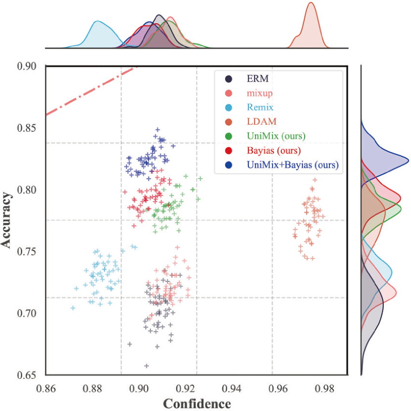
(a) CIFAR-10-LT-100

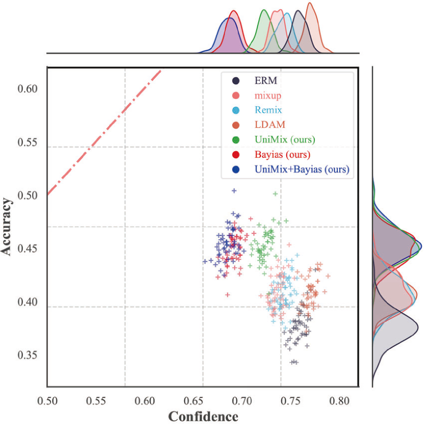
(b) CIFAR-100-LT-100

Figure D2: Additional comparisons of joint density plots of accuracy vs. confidence on CIFAR-10-LT and CIFAR-100-LT. A well-calibrated classifier’s density will lay around the $y=x$ (red dot line). The combination of UniMix and Bayias achieves remarkable results especially in the severely imbalance scenarios (i.e., $\rho=100$).

Fig.D2 clearly shows that the proposed method achieves better calibration in the CIFAR-LT test set. Each scatters data is the corresponding result of confidence and accuracy in a mini-batch $m$. In LT scenarios, the validation accuracy is usually lower than train accuracy, especially for the tail classes. Such overconfidence and miscalibration obstruct the network from having better generalization performance. In Fig.D2, the distribution of scattered points reflects a model’s generalization and calibration. Our proposed method is the closest towards ideal $y=x$. It means each class gets enough regulation and hence contributes to a well-calibrated model. In contrast, mixup and its extensions are similar to ERM, which show limited improvement on classification calibration in LT scenarios. LDAM ameliorates the LT situation to some extent but results in more severe overconfidence cases, which may explain why it is counterproductive to other methods.

The reliability diagram is another visual representation of model calibration. As Fig.LABEL:Fig.addcifar-10-100-bar shows, the baseline (ERM) is overconfident in its predictions and the accuracy is generally below ideal $y=x$ for each bin. Our method produces much better confidence estimates than others, which means our success in regulating all classes. Although some post-hoc adjustment methods [18, 68] can achieve better classification calibration, our approach trains a calibrated model end-to-end, which avoids the potential adverse effects on the original task. Considering the similarity of purposes with MiSLAS [68], we make detailed discussion in Appendix D.5.

D.3 Additional visualized comparisons of confusion matrix on CIFAR-LT

D.3.1 Visualized confusion matrix on CIFAR-10-LT

We further give additional visualized results on CIFAR-10-LT setting $\rho=10$ and $\rho=100$, which are available in Fig.D4,D5. The results show that all methods perform well compared with ERM in the simple dataset (e.g., CIFAR-10-LT-10, CIFAR-10-LT-100). In general, the proposed method significantly improves the accuracy of the tail for the larger diagonal values. The improvement on the tail is superior than other methods, which leads to state-of-the-art performance.

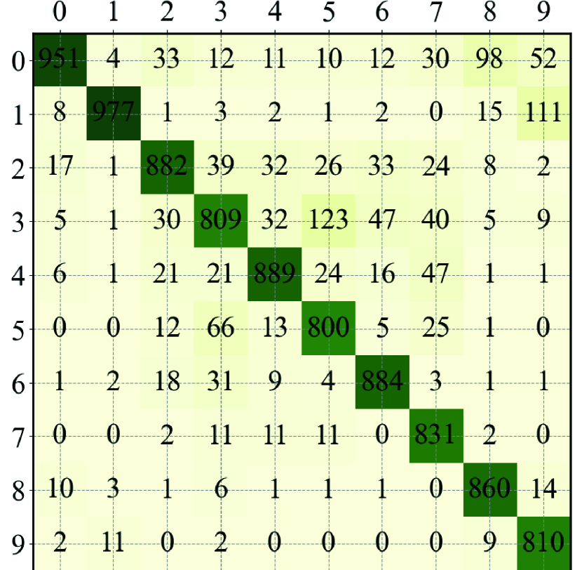
(a) ERM

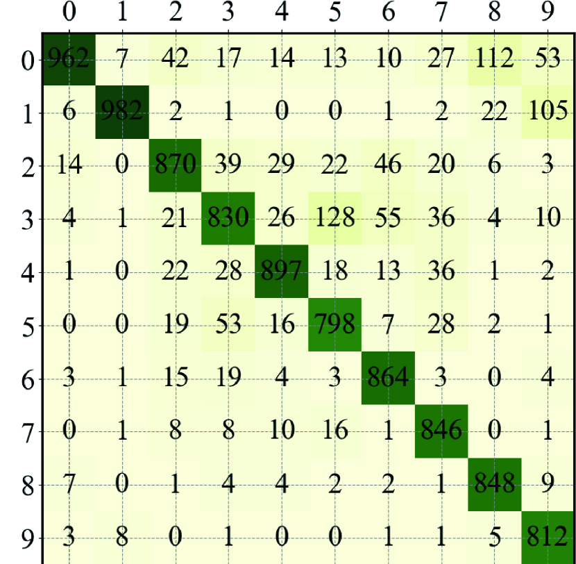
(b) mixup [64]

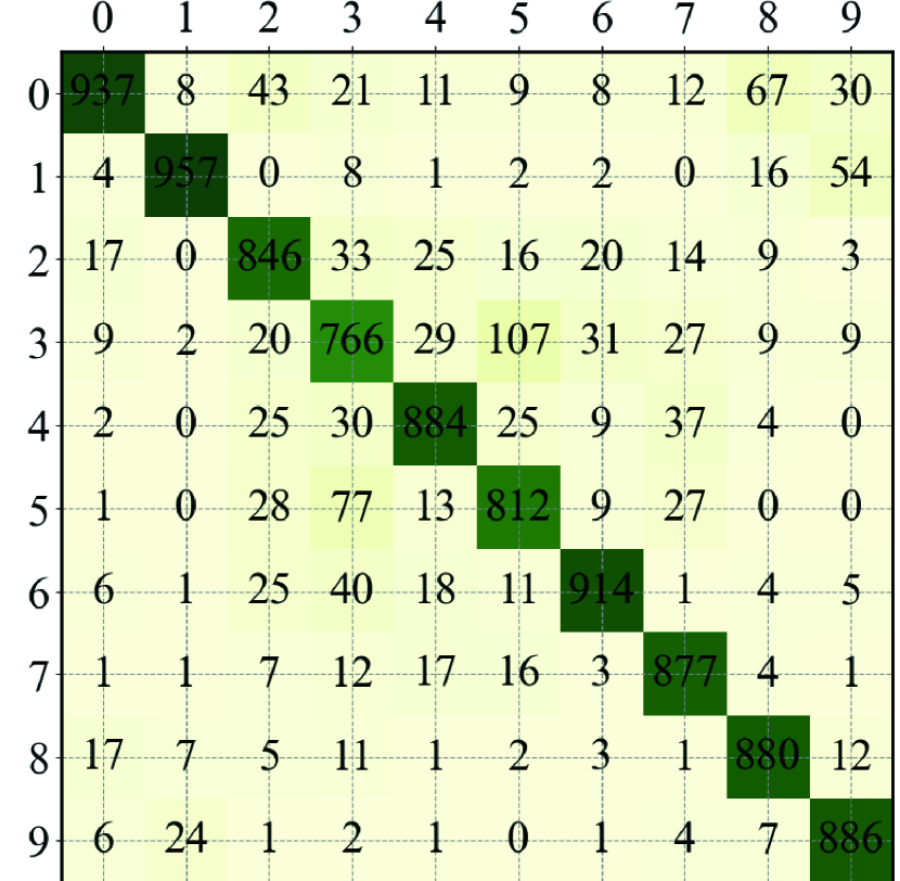
(c) LDAM+DRW [8]

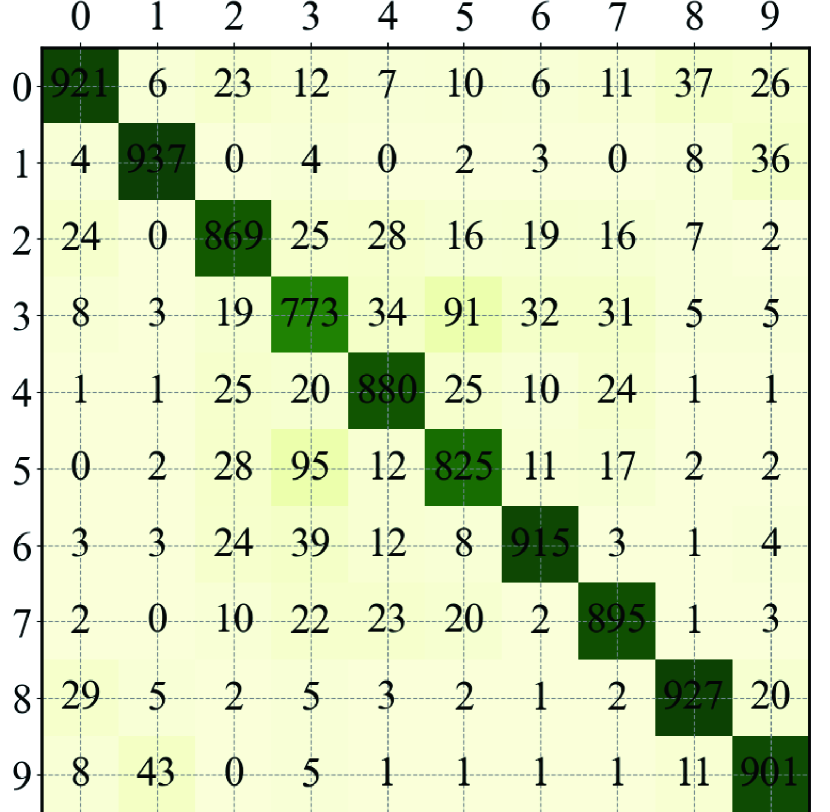
(d) CDT [62]

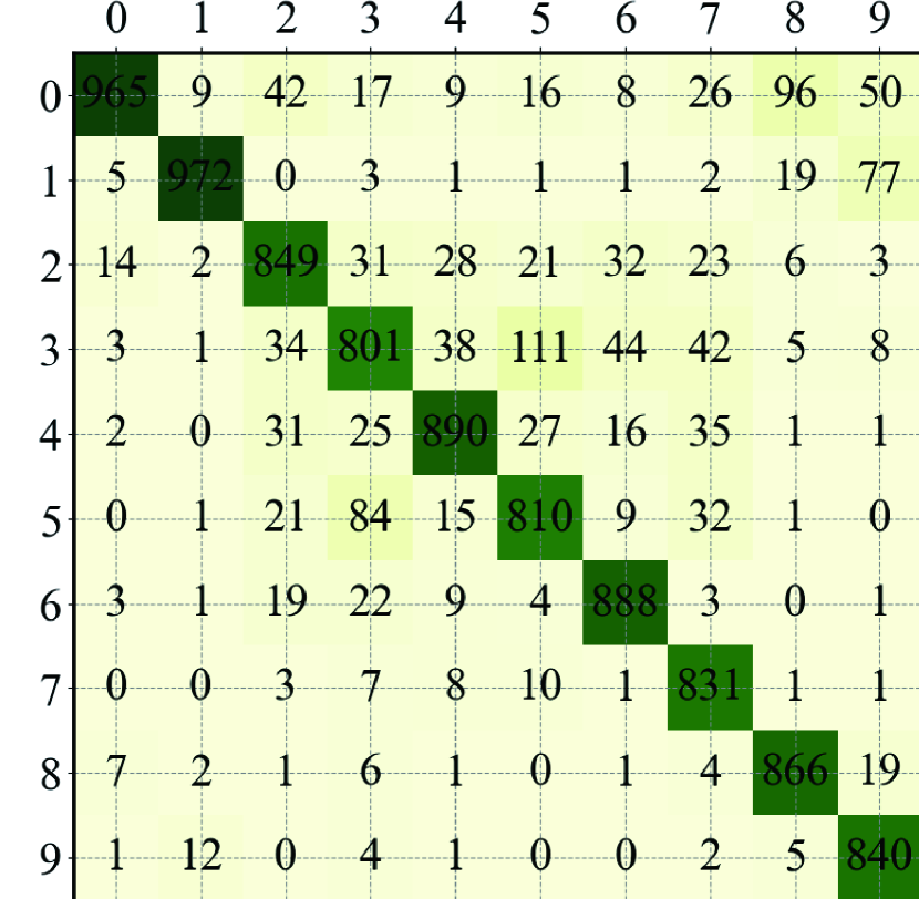
(e) Remix [12]

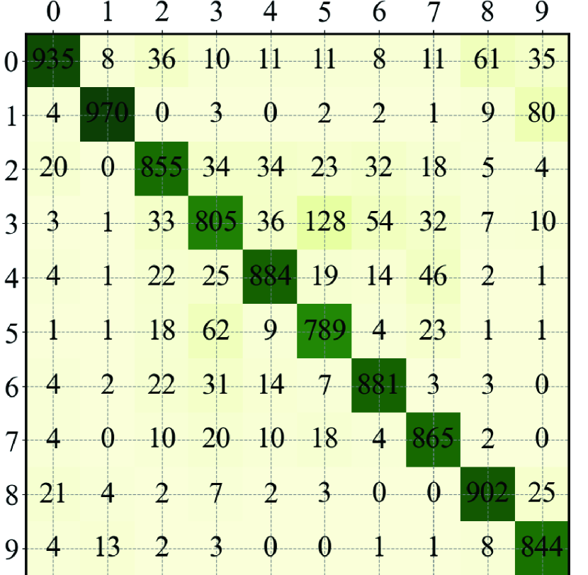
(f) CB+DRW [14]

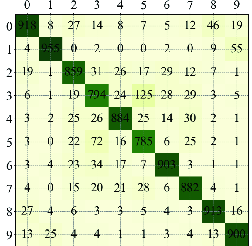
(g) Logit Adjustment [47]

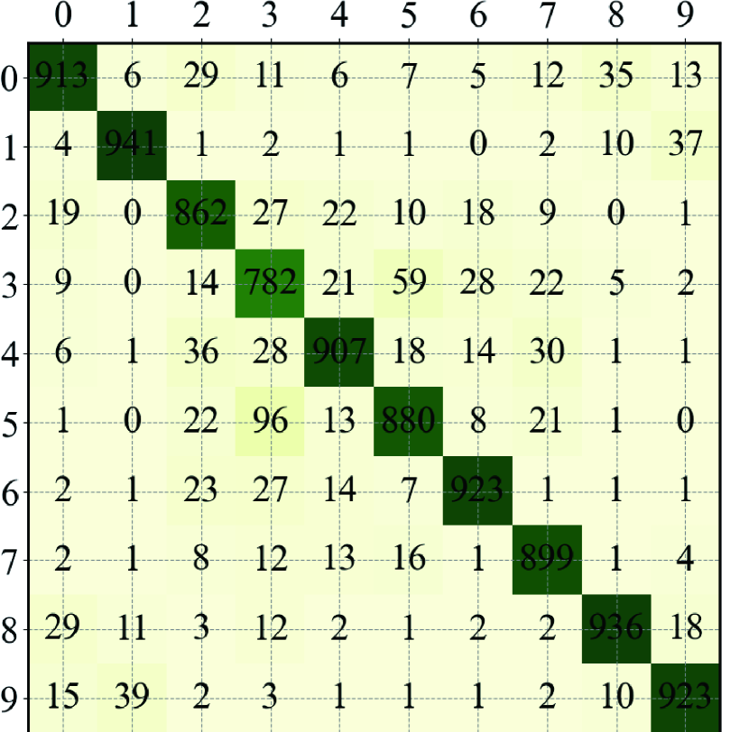
(h) Ours

Figure D4: Additional confusion matrix comparisons on CIFAR-10-LT-10. The $x$-axis and $y$-axis indicate the ground truth and predicted labels, respectively. Deeper color indicates larger values. All methods achieve satisfactory results while ours further improves the tail feature learning and make misclassification cases more balanced distributed.

As for misclassification results, the non-diagonal elements concentrate on the top-right triangle. Hence, most of previous methods have limited improvement on minority classes, which tend to simply predict the instances in tail as majority ones. In contrast, the proposed method improves the performance for the tail and makes the misclassification case more balance distributed.

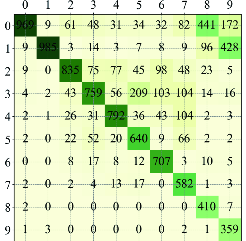
(a) ERM

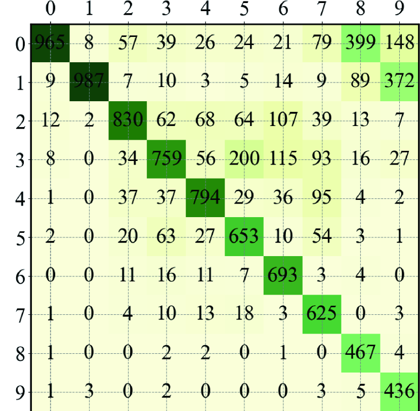
(b) mixup [64]

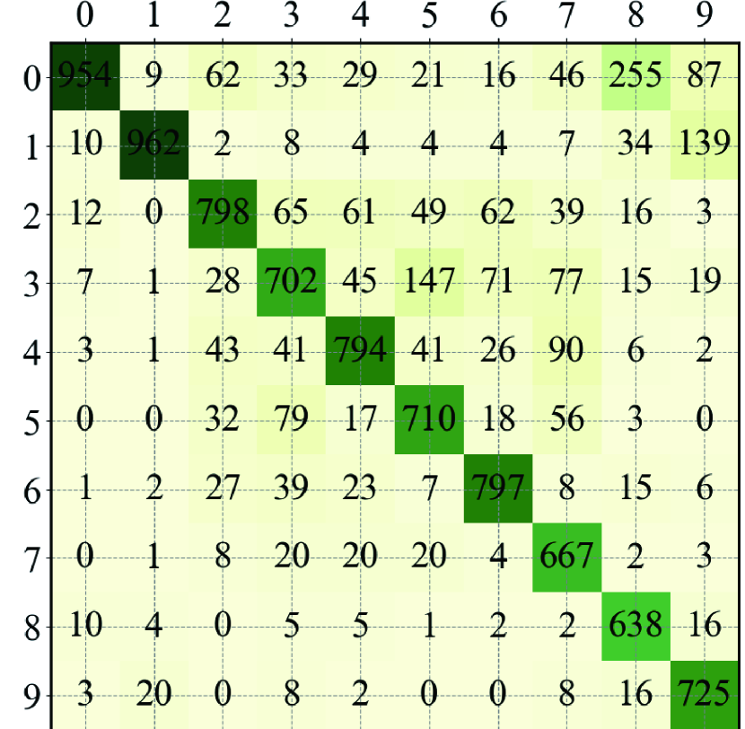
(c) LDAM+DRW [8]

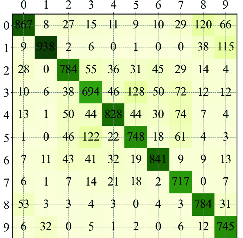
(d) CDT [62]

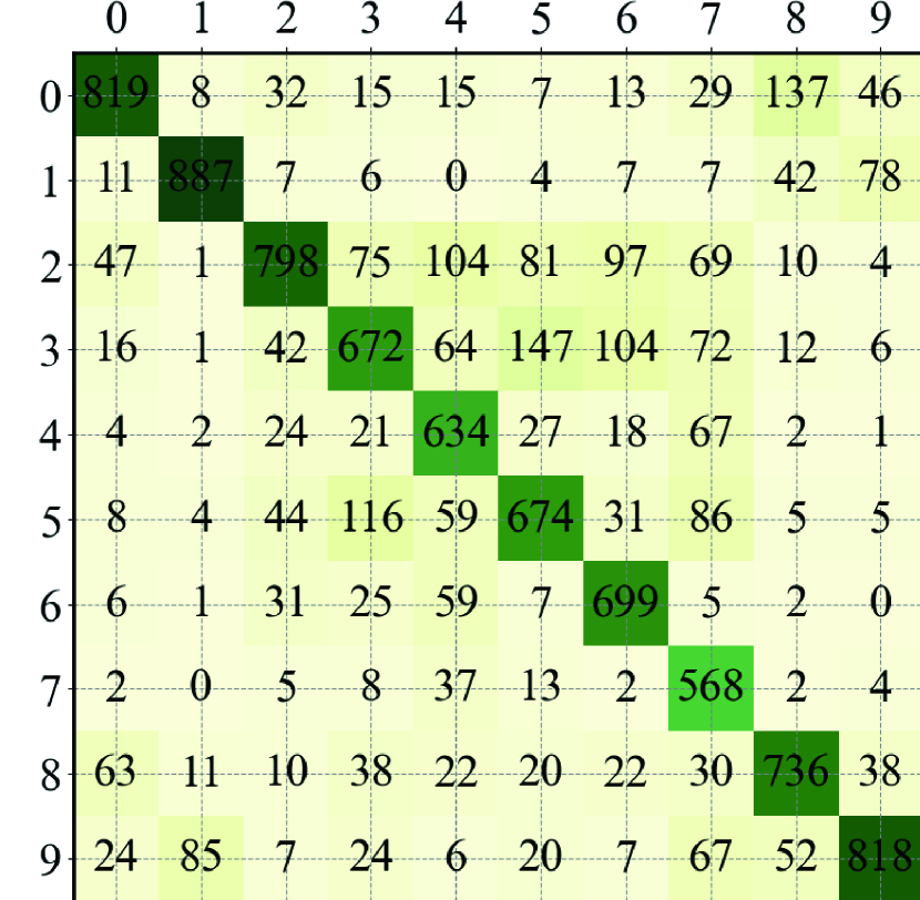
(e) Remix [12]

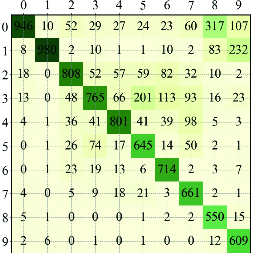
(f) CB+DRW [14]

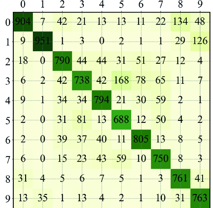
(g) Logit Adjustment [47]

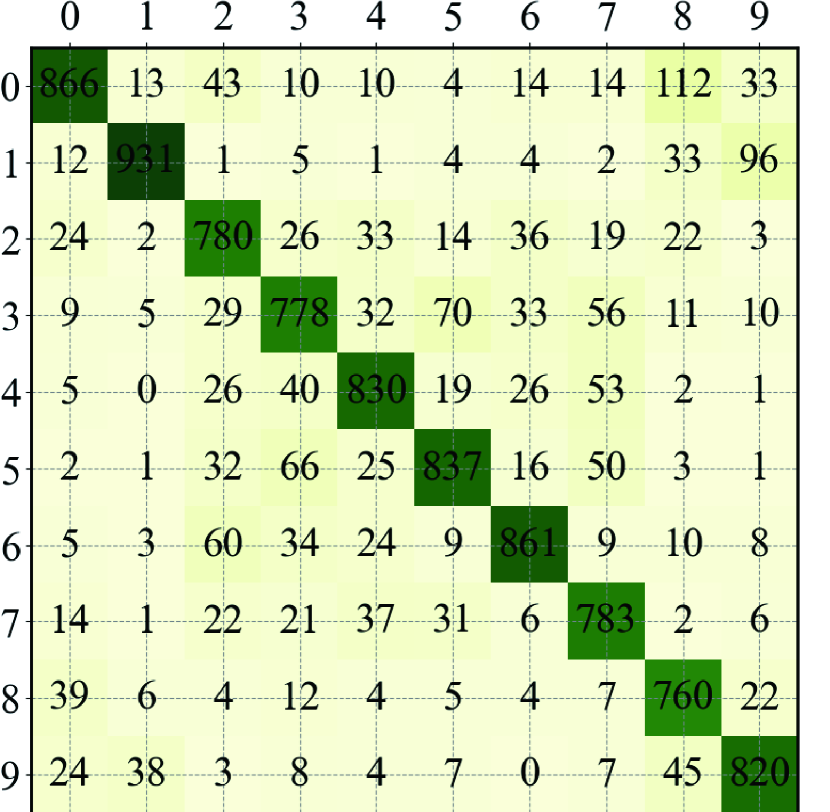
(h) Ours

Figure D5: Additional confusion matrix comparisons on CIFAR-10-LT-100. The $x$-axis and $y$-axis indicate the ground truth and predicted labels, respectively. Deeper color indicates larger values. The disparity of these methods gradually gets appeared. Our method achieves the best accuracy as well as better non-diagonal distribution. Other methods exhibit an obvious bias towards the head or tail.

D.3.2 Visualized $\log$-confusion matrix on CIFAR-100-LT

Furthermore, we visualize the distinguishing results of our methods on challenging CIFAR-100-LT for comprehensive comparisons. Specifically, we plot additional comparisons on CIFAR-100-LT-10 (Fig.D6) and CIFAR-100-LT-100 (Fig.D7).

Fig.D6 D7 show that in the challenging LT scenarios, the diagonal values get decreased towards the tail. A proper confusion matrix should exhibit a balanced distribution of misclassification case and large enough diagonal values. The proposed method outperforms others both in the correct cases (the diagonal elements) and the misclassification case distribution. In general, the proposed method shows the best performance, especially in the tail classes (deeper color represents larger value). The misclassification cases in other methods apparently concentrate on the upper triangular, which means the classifiers simply predict the tail samples as the head and vise versa.

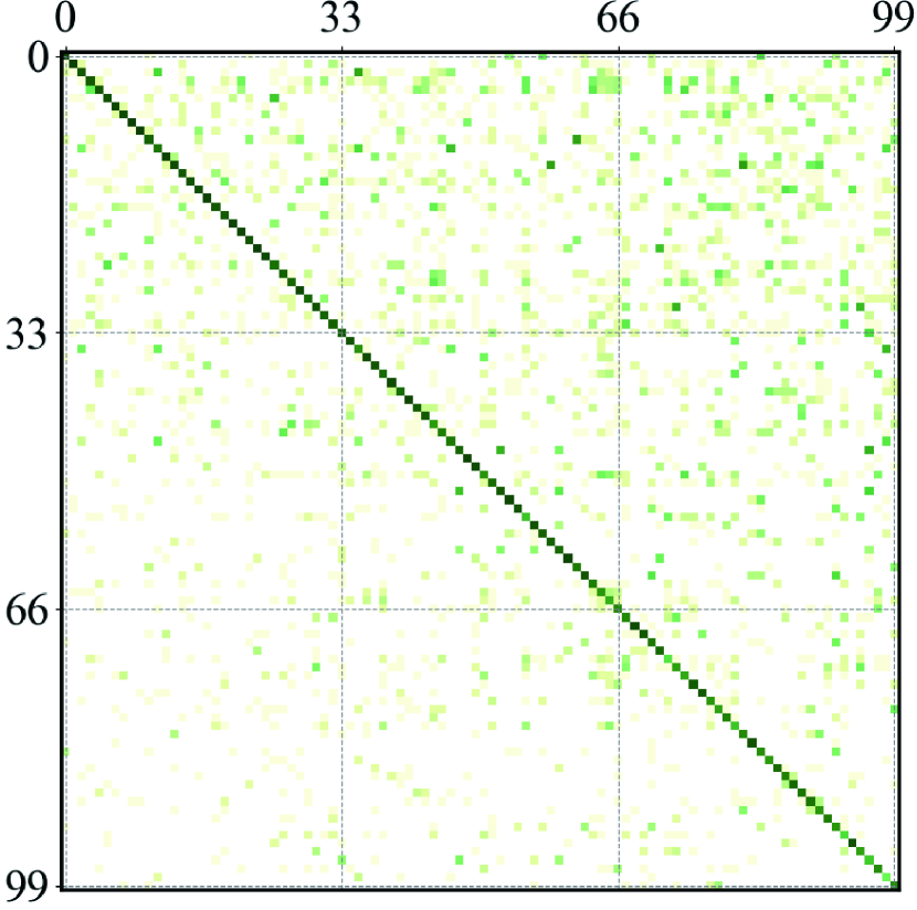
(a) ERM

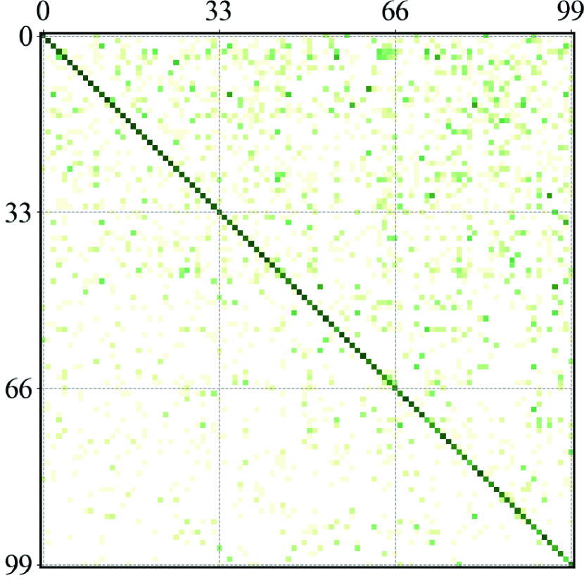
(b) mixup [64]

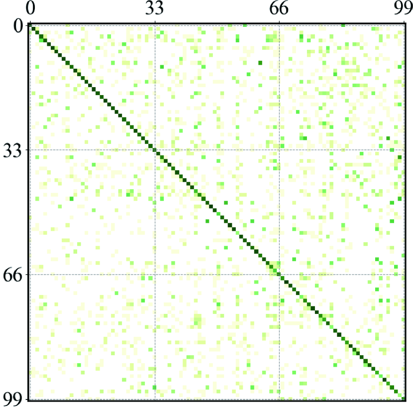
(c) LDAM+DRW [8]

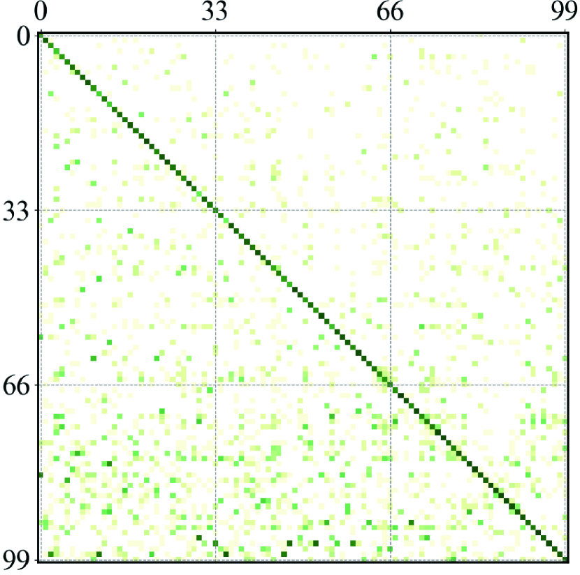
(d) CDT [62]

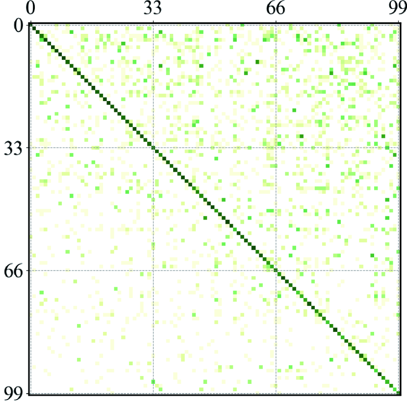
(e) Remix [12]

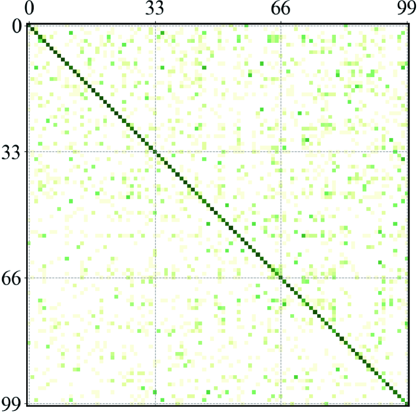
(f) CB+DRW [14]

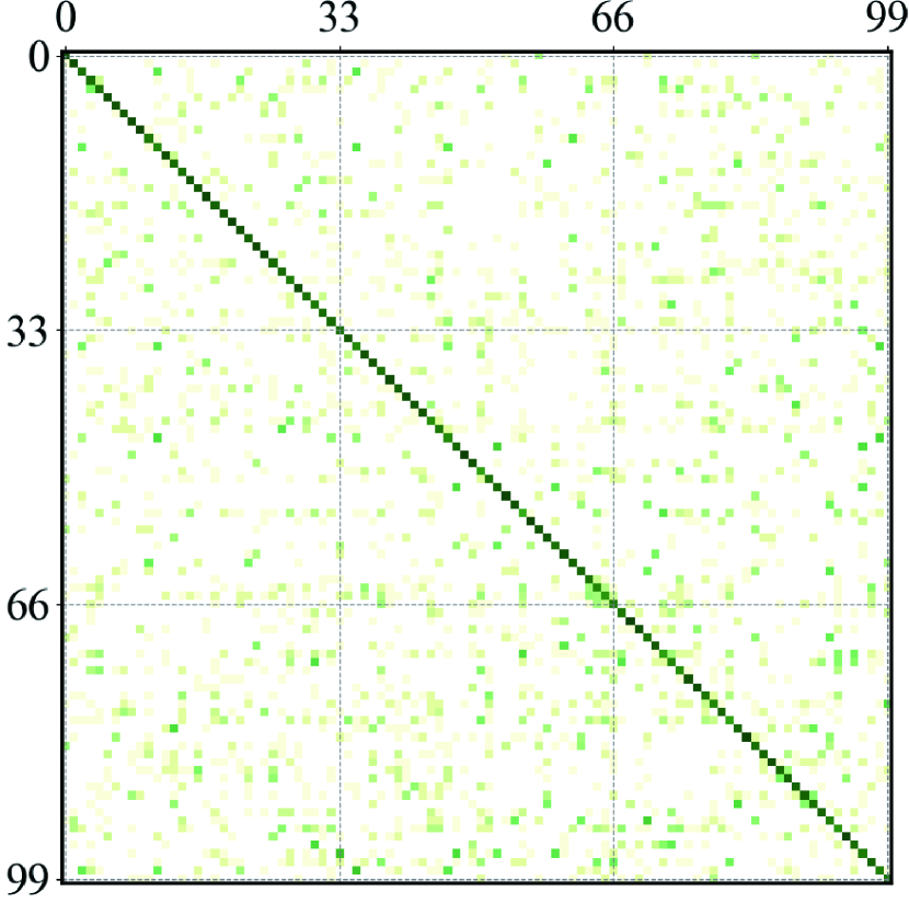
(g) Logit Adjustment [47]

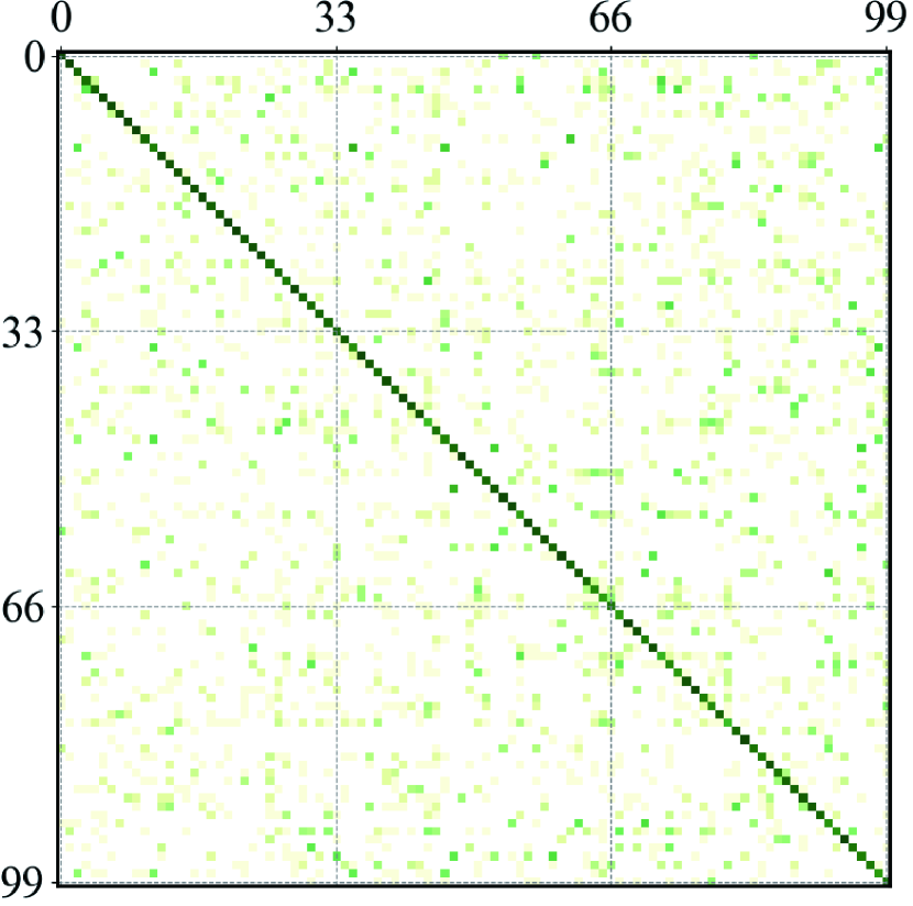
(h) Ours

Figure D6: Additional $\log$-confusion matrix comparisons on CIFAR-100-LT-10. The $x$-axis and $y$-axis indicate the ground truth and predicted labels, respectively. $\log$ operation is adopted for clearer visualisation. Deeper color indicates larger values. The increased class number makes the misclassification distribution more clearly.

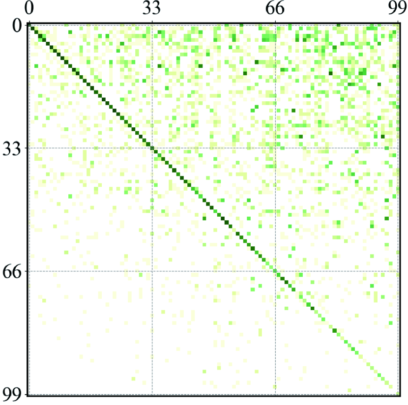
(a) ERM

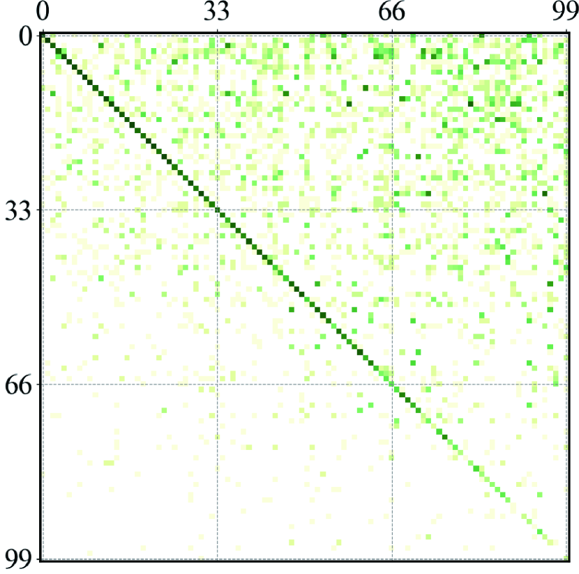
(b) mixup [64]

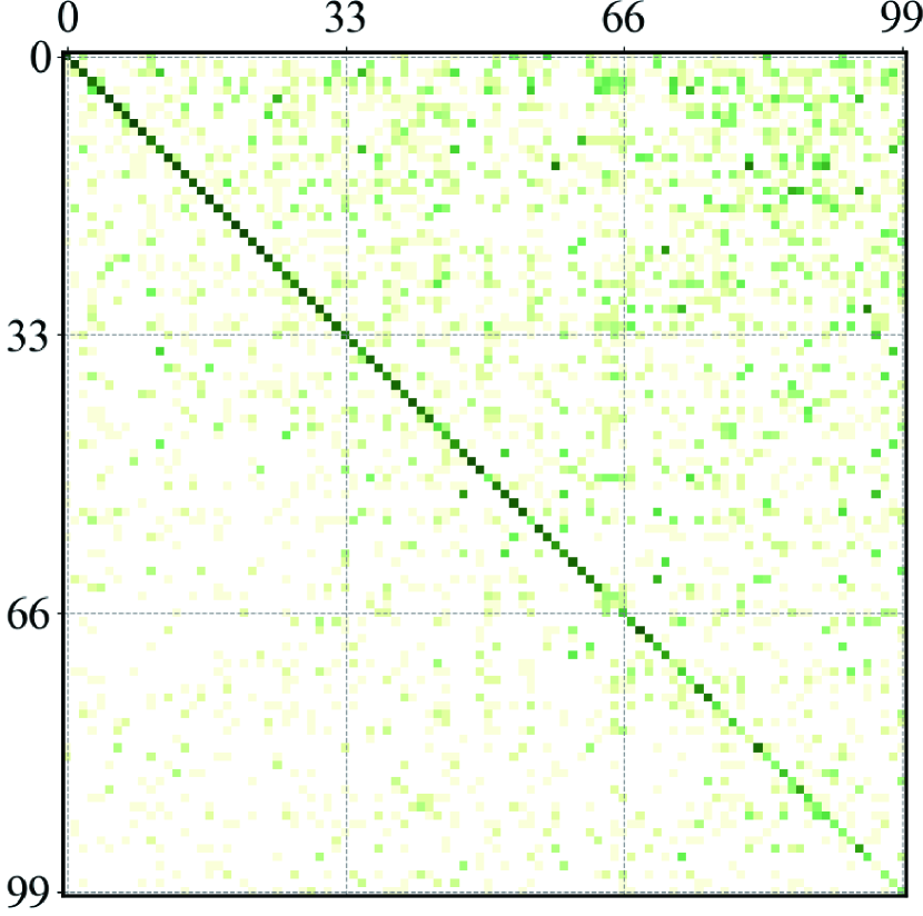
(c) LDAM+DRW [8]

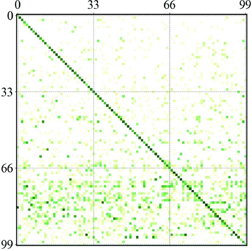
(d) CDT [62]

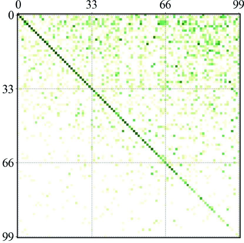
(e) Remix [12]

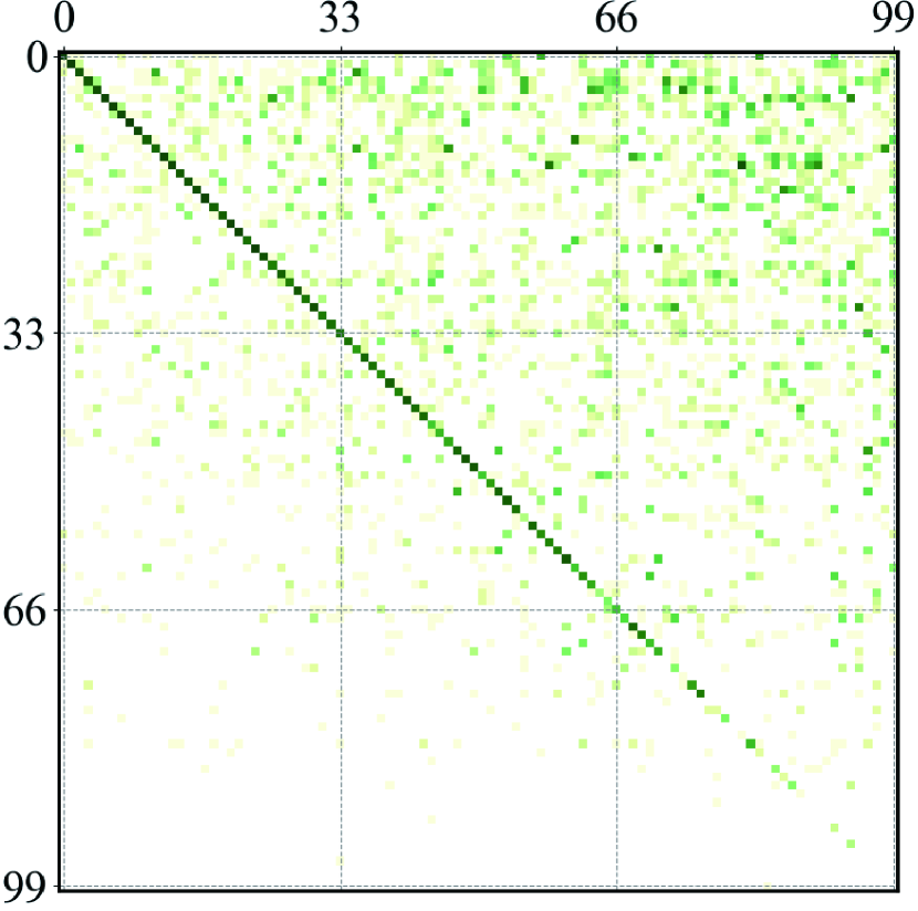
(f) CB+DRW [14]

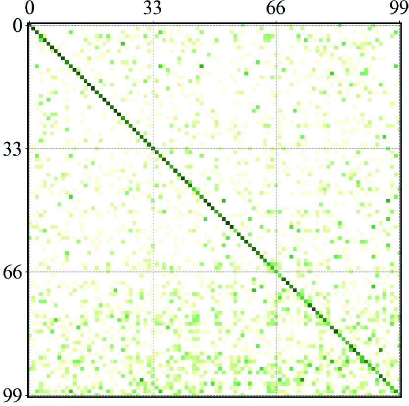
(g) Logit Adjustment [47]

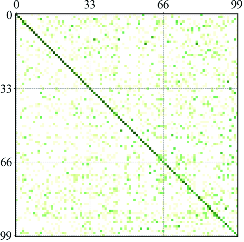
(h) Ours

Figure D7: Additional $\log$-confusion matrix comparisons on CIFAR-100-LT-100. The $x$-axis and $y$-axis indicate the ground truth and predicted labels, respectively. $\log$ operation is adopted for clearer comparisons. Deeper color indicates larger values. Other methods show obviously poor generalization on the tail in the challenging CIFAR-100-LT-100, while the proposed method achieves significantly superior correct classification results and balanced misclassification case distribution.

D.4 Results on test imbalance scenarios

Zhang et al. [66] have discussed the existing challenging and severe bias issue in imbalanced distributed test set. When the test set distribution is ideally known or well estimated, Bayias enables to overcome the bias issues in such scenarios by considering the priors. In contrast, CE loss implicitly requires train set and test set same distributed, while LA loss requires test set balanced distributed. LA and CE losses are powerless in other scenarios, while Bayias is flexible and capable with imbalanced distributed test sets, i.e., the constant term $\log C$ can change to be the test set distribution $\log\pi^{\prime}$ to deal with such scenarios.

We sample test sets under different distribution with test imbalance factor $\rho^{\prime}$ (i.e., long-tail ($\rho^{\prime}>1$), balanced ($\rho^{\prime}=1$), and reversed long-tail ($\rho^{\prime}<1$)), corresponding to different imbalance factor $100,10,1,0.1,0.01$. The following comparisons in Tab.D2 show the necessity of considering test distribution’s influence, which reveals our motivation to deal with bias issues. When train and test sets follow the same distribution, Bayias is equal to CE and outperforms LA. When the distribution of train and test set is different severely (e.g., $\rho^{\prime}=100$ and $0.01$), Bayias outperforms both CE and LA. Similar experiments and conclusions can be obtained from [27] as well.

Table D2: Comparisons of CE, LA and Bayias loss on CIFAR-100-LT class-imbalanced test set. Note that the imbalanced test set is sampled by discarding some data. Therefore, the instance numbers of test samples vary in different imbalance factors, and longitudinal comparisons can reflect the effectiveness of Bayias.

Train set	CIFAR-100-LT-10					CIFAR-100-LT-100
$\rho^{\prime}$	100	10	1	0.1	0.01	100	10	1	0.1	0.01
CE	69.73	63.67	55.70	48.48	43.13	63.54	52.74	38.32	25.00	14.03
LA	61.94	60.14	59.87	56.12	54.06	59.13	51.06	43.89	31.14	26.42
Bayias	71.89	63.36	60.02	58.20	62.32	64.90	54.15	43.92	36.20	35.42

D.5 Comparisons with the two-stage method

We propose UniMix and Bayias to improve model calibration by tackling the bias issues caused by imbalanced distributed train and test set. We improve the model calibration and accuracy simultaneously in an end-to-end manner. However, there are some methods to ameliorate calibration in post-hoc (e.g., temperature scaling [18]) or two-stage (e.g., label aware smoothing [68]) way. As we discussed above, such pipelines will be effective and we integrate our proposed methods with one of them for further comparison. The compared results are illustrated in Tab.D3.

Table D3: Comparisons with state-of-the-art two-stage method on CIFAR-100-LT.

Dataset		CIFAR-100-LT-10		CIFAR-100-LT-50		CIFAR-100-LT-100
Metric (%)		Accuracy	ECE	Accuracy	ECE	Accuracy	ECE
MiSLAS	1st-stage	58.7	3.91	45.6	6.00	40.3	10.77
	2nd-stage	63.2	1.73	52.3	2.25	47.0	4.83
Ours	1st-stage	61.1	7.79	51.8	4.91	47.6	3.24
	2nd-stage	63.0	1.98	52.6	3.45	48.3	1.44

MiSLAS adopts mixup for the 1st-stage and label aware smoothing (LAS) for 2nd-stage. We add the LAS in additional $10$ epochs following our vanilla pipeline to build a two-stage manner. Our method generally outperforms MiSLAS in the 1st-stage and can achieve on par with accuracy and lower ECE. In specific, MiSLAS mainly improves accuracy and ECE in the 2nd-stage, i.e., classifier learning, by a large margin, which indicates LAS’s effectiveness. We adopt the LAS to replace Bayias compensated CE loss in the 2nd-stage and can further improve accuracy and ECE, especially in the more challenging CIFAR-100-LT-100. However, the improvement of the 2nd-stage is not significant compared to MiSLAS. Since the LAS and Bayias compensated CE loss are both modifications on standard CE loss, it is hard to implement both of them simultaneously. We suggest that the LAS plays similar roles as Bayias compensated CE loss does, which explains the limited performance improvement.

Appendix E Additional discussion

What is the difference between UniMix and traditional over-sample approaches? We take representative over-sample approach SMOTE [11] for comparisons. SMOTE is a classic over-sample method for imbalanced data learning, which constructs synthetic data via interpolation among a sample’s neighbors in the same class. However, the authors in [58] illustrate that such interpolation without labels is negative for classification calibration. In contrast, mixup manners take elaborate-designed label mix strategies. The success of label smoothing trick [25] and mixups imply that the fusion of label may play an important role in classification accuracy and calibration. Different from other methods, our UniMix pays more attention to the tail when mixing the label and thus achieves remarkable performance gain.

Why choose $\bm{\xi^{*}_{i,j}\sim\mathscr{U}(\pi_{y_{i}},\pi_{y_{j}},\alpha,\alpha)}$? As we have discussed the motivation of UniMix Factor before, it is intuitive to set $\xi_{i,j}=\pi_{y_{j}}/(\pi_{y_{i}}+\pi_{y_{j}})$. Although satisfactory performance gain is obtained on CIFAR-LT in this manner, we fail on large-scaled dataset like ImageNet-LT. We suspect that the $\xi^{*}_{i,j}$ will be close to $0$ or $1$ when the datasets become extremely imbalanced and hence the effect of our mixing manner disappears. To improve the robustness and generalization, we transform the origin $Beta(\alpha,\alpha)$ distribution ($\alpha\leq 1$) to maximize the probability of $\xi_{i,j}=\pi_{y_{j}}/(\pi_{y_{i}}+\pi_{y_{j}})$ and its vicinity. We set $\alpha=0.5$ on CIFAR-LT and keep the same $\alpha$ as mixup and Remix on ImageNet-LT and iNaturalist 2018.

Why does Bayias work? According to Bayesian theory, the estimated likelihood is positive correlation to posterior both in balance-distributed train and test set, with the same constant coefficient of prior and evidence factor. However, though evidence factor is regraded as a constant in LT scenarios, the LT dataset suffers seriously skewed prior of each category in the train set, which is extremely different from the balanced test set. Hence, the model based on maximizing posterior probability needs the to compensate the different priors firstly. From the perspective of optimization, Deep Neural Network (DNN) is a non-convex model, minuscule bias will eventually cause disturbances in the optimization direction, resulting in parameters converging to another local optimal. In addition, $\log(\pi_{i})+\log(C)$ is consistent with traditional balanced datasets (i.e., $\pi_{i}\equiv 1/C$), which turns to be a special case (i.e., $\log(1/C)+\log(C)\equiv 0$) of Bayias. Furthermore, our Bayias can compensate any discrepancy between train set and test set via directly setting the Bayias as $\log(\pi_{y_{i}})-\log(\pi^{\prime}_{y_{i}})$, where $\pi_{y_{i}}$ is the label prior in train set and $\pi^{\prime}_{y_{i}}$ is the label prior in test set.

References

- [1] Marcin Andrychowicz, Misha Denil, Sergio Gomez Colmenarejo, Matthew W. Hoffman, David Pfau, Tom Schaul, and Nando de Freitas. Learning to learn by gradient descent by gradient descent. In Advances in Neural Information Processing Systems 29: Annual Conference on Neural Information Processing Systems 2016, pages 3981–3989, 2016.
- [2] Arsenii Ashukha, Alexander Lyzhov, Dmitry Molchanov, and Dmitry P. Vetrov. Pitfalls of in-domain uncertainty estimation and ensembling in deep learning. In 8th International Conference on Learning Representations, ICLR 2020. OpenReview.net, 2020.
- [3] Peter L Bartlett, Michael I Jordan, and Jon D McAuliffe. Convexity, classification, and risk bounds. Journal of the American Statistical Association, 101(473):138–156, 2006.
- [4] Mariusz Bojarski, Davide Del Testa, Daniel Dworakowski, Bernhard Firner, Beat Flepp, Prasoon Goyal, Lawrence D. Jackel, Mathew Monfort, Urs Muller, Jiakai Zhang, Xin Zhang, Jake Zhao, and Karol Zieba. End to end learning for self-driving cars. CoRR, abs/1604.07316, 2016.
- [5] Glenn W Brier et al. Verification of forecasts expressed in terms of probability. Monthly weather review, 78(1):1–3.
- [6] Mateusz Buda, Atsuto Maki, and Maciej A. Mazurowski. A systematic study of the class imbalance problem in convolutional neural networks. Neural Networks, 106:249–259, 2018.
- [7] Jonathon Byrd and Zachary Chase Lipton. What is the effect of importance weighting in deep learning? In Proceedings of the 36th International Conference on Machine Learning, ICML 2019, volume 97 of Proceedings of Machine Learning Research, pages 872–881. PMLR, 2019.
- [8] Kaidi Cao, Colin Wei, Adrien Gaidon, Nikos Aréchiga, and Tengyu Ma. Learning imbalanced datasets with label-distribution-aware margin loss. In Advances in Neural Information Processing Systems NeurIPS 2019, pages 1565–1576, 2019.
- [9] Rich Caruana, Yin Lou, Johannes Gehrke, Paul Koch, Marc Sturm, and Noemie Elhadad. Intelligible models for healthcare: Predicting pneumonia risk and hospital 30-day readmission. In Proceedings of the 21th ACM SIGKDD International Conference on Knowledge Discovery and Data Mining, pages 1721–1730. ACM, 2015.
- [10] Olivier Chapelle, Jason Weston, Léon Bottou, and Vladimir Vapnik. Vicinal risk minimization. In Advances in Neural Information Processing Systems 13, Papers from Neural Information Processing Systems (NIPS) 2000, Denver, CO, USA, pages 416–422. MIT Press, 2000.
- [11] Nitesh V. Chawla, Kevin W. Bowyer, Lawrence O. Hall, and W. Philip Kegelmeyer. SMOTE: synthetic minority over-sampling technique. J. Artif. Intell. Res., 16:321–357, 2002.
- [12] Hsin-Ping Chou, Shih-Chieh Chang, Jia-Yu Pan, Wei Wei, and Da-Cheng Juan. Remix: Rebalanced mixup. In Computer Vision - ECCV 2020 Workshops, volume 12540, pages 95–110. Springer, 2020.
- [13] Peng Chu, Xiao Bian, Shaopeng Liu, and Haibin Ling. Feature space augmentation for long-tailed data. In Computer Vision - ECCV 2020 - 16th European Conference, volume 12374 of Lecture Notes in Computer Science, pages 694–710. Springer, 2020.
- [14] Yin Cui, Menglin Jia, Tsung-Yi Lin, Yang Song, and Serge J. Belongie. Class-balanced loss based on effective number of samples. In IEEE Conference on Computer Vision and Pattern Recognition, CVPR 2019, pages 9268–9277. Computer Vision Foundation / IEEE, 2019.
- [15] Jiankang Deng, Jia Guo, Niannan Xue, and Stefanos Zafeiriou. Arcface: Additive angular margin loss for deep face recognition. In IEEE Conference on Computer Vision and Pattern Recognition, CVPR 2019, pages 4690–4699. Computer Vision Foundation / IEEE, 2019.
- [16] Theodoros Evgeniou and Massimiliano Pontil. Support vector machines: Theory and applications. In Machine Learning and Its Applications, Advanced Lectures, volume 2049 of Lecture Notes in Computer Science, pages 249–257. Springer, 2001.
- [17] Chelsea Finn, Pieter Abbeel, and Sergey Levine. Model-agnostic meta-learning for fast adaptation of deep networks. In Proceedings of the 34th International Conference on Machine Learning, ICML 2017, volume 70 of Proceedings of Machine Learning Research, pages 1126–1135. PMLR, 2017.
- [18] Chuan Guo, Geoff Pleiss, Yu Sun, and Kilian Q. Weinberger. On calibration of modern neural networks. In Proceedings of the 34th International Conference on Machine Learning, ICML 2017, volume 70 of Proceedings of Machine Learning Research, pages 1321–1330. PMLR, 2017.
- [19] Agrim Gupta, Piotr Dollár, and Ross B. Girshick. LVIS: A dataset for large vocabulary instance segmentation. In IEEE Conference on Computer Vision and Pattern Recognition, CVPR 2019, pages 5356–5364. Computer Vision Foundation / IEEE, 2019.
- [20] Hui Han, Wenyuan Wang, and Binghuan Mao. Borderline-smote: A new over-sampling method in imbalanced data sets learning. In Advances in Intelligent Computing, International Conference on Intelligent Computing, ICIC 2005, volume 3644 of Lecture Notes in Computer Science, pages 878–887. Springer, 2005.
- [21] Munawar Hayat, Salman H. Khan, Syed Waqas Zamir, Jianbing Shen, and Ling Shao. Gaussian affinity for max-margin class imbalanced learning. In 2019 IEEE/CVF International Conference on Computer Vision, ICCV 2019, pages 6468–6478. IEEE, 2019.
- [22] Haibo He and Edwardo A. Garcia. Learning from imbalanced data. IEEE Trans. Knowl. Data Eng., 21(9):1263–1284, 2009.
- [23] Kaiming He, Georgia Gkioxari, Piotr Dollár, and Ross B. Girshick. Mask R-CNN. In IEEE International Conference on Computer Vision, ICCV 2017, pages 2980–2988. IEEE Computer Society, 2017.
- [24] Kaiming He, Xiangyu Zhang, Shaoqing Ren, and Jian Sun. Deep residual learning for image recognition. In 2016 IEEE Conference on Computer Vision and Pattern Recognition, CVPR 2016, pages 770–778. IEEE Computer Society, 2016.
- [25] Tong He, Zhi Zhang, Hang Zhang, Zhongyue Zhang, Junyuan Xie, and Mu Li. Bag of tricks for image classification with convolutional neural networks. In IEEE Conference on Computer Vision and Pattern Recognition, CVPR 2019, pages 558–567. Computer Vision Foundation / IEEE, 2019.
- [26] Zhuoxun He, Lingxi Xie, Xin Chen, Ya Zhang, Yanfeng Wang, and Qi Tian. Data augmentation revisited: Rethinking the distribution gap between clean and augmented data. CoRR, abs/1909.09148, 2019.
- [27] Youngkyu Hong, Seungju Han, Kwanghee Choi, Seokjun Seo, Beomsu Kim, and Buru Chang. Disentangling label distribution for long-tailed visual recognition. In Proceedings of the IEEE/CVF Conference on Computer Vision and Pattern Recognition, pages 6626–6636.
- [28] Grant Van Horn, Oisin Mac Aodha, Yang Song, Yin Cui, Chen Sun, Alexander Shepard, Hartwig Adam, Pietro Perona, and Serge J. Belongie. The inaturalist species classification and detection dataset. In 2018 IEEE Conference on Computer Vision and Pattern Recognition, CVPR 2018, pages 8769–8778. IEEE Computer Society, 2018.
- [29] Grant Van Horn and Pietro Perona. The devil is in the tails: Fine-grained classification in the wild. CoRR, abs/1709.01450, 2017.
- [30] Chen Huang, Yining Li, Chen Change Loy, and Xiaoou Tang. Learning deep representation for imbalanced classification. In 2016 IEEE Conference on Computer Vision and Pattern Recognition, CVPR 2016, pages 5375–5384. IEEE Computer Society, 2016.
- [31] Chen Huang, Yining Li, Chen Change Loy, and Xiaoou Tang. Deep imbalanced learning for face recognition and attribute prediction. IEEE Trans. Pattern Anal. Mach. Intell., 42(11):2781–2794, 2020.
- [32] Muhammad Abdullah Jamal, Matthew Brown, Ming-Hsuan Yang, Liqiang Wang, and Boqing Gong. Rethinking class-balanced methods for long-tailed visual recognition from a domain adaptation perspective. In 2020 IEEE/CVF Conference on Computer Vision and Pattern Recognition, CVPR 2020, pages 7607–7616. IEEE, 2020.
- [33] Bingyi Kang, Saining Xie, Marcus Rohrbach, Zhicheng Yan, Albert Gordo, Jiashi Feng, and Yannis Kalantidis. Decoupling representation and classifier for long-tailed recognition. In 8th International Conference on Learning Representations, ICLR 2020. OpenReview.net, 2020.
- [34] Salman H. Khan, Munawar Hayat, Mohammed Bennamoun, Ferdous Ahmed Sohel, and Roberto Togneri. Cost-sensitive learning of deep feature representations from imbalanced data. IEEE Trans. Neural Networks Learn. Syst., 29(8):3573–3587, 2018.
- [35] Salman H. Khan, Munawar Hayat, Syed Waqas Zamir, Jianbing Shen, and Ling Shao. Striking the right balance with uncertainty. In IEEE Conference on Computer Vision and Pattern Recognition, CVPR 2019, pages 103–112. Computer Vision Foundation / IEEE, 2019.
- [36] Jaehyung Kim, Jongheon Jeong, and Jinwoo Shin. M2m: Imbalanced classification via major-to-minor translation. In 2020 IEEE/CVF Conference on Computer Vision and Pattern Recognition, CVPR 2020, pages 13893–13902. IEEE, 2020.
- [37] Ranjay Krishna, Yuke Zhu, Oliver Groth, Justin Johnson, Kenji Hata, Joshua Kravitz, Stephanie Chen, Yannis Kalantidis, Li-Jia Li, David A. Shamma, Michael S. Bernstein, and Li Fei-Fei. Visual genome: Connecting language and vision using crowdsourced dense image annotations. Int. J. Comput. Vis., 123(1):32–73, 2017.
- [38] Alex Krizhevsky, Geoffrey Hinton, et al. Learning multiple layers of features from tiny images. 2009.
- [39] Buyu Li, Yu Liu, and Xiaogang Wang. Gradient harmonized single-stage detector. In The Thirty-Third AAAI Conference on Artificial Intelligence, AAAI 2019, pages 8577–8584. AAAI Press, 2019.
- [40] Yu Li, Tao Wang, Bingyi Kang, Sheng Tang, Chunfeng Wang, Jintao Li, and Jiashi Feng. Overcoming classifier imbalance for long-tail object detection with balanced group softmax. In Proceedings of the IEEE/CVF Conference on Computer Vision and Pattern Recognition, pages 10991–11000, 2020.
- [41] Tsung-Yi Lin, Priya Goyal, Ross B. Girshick, Kaiming He, and Piotr Dollár. Focal loss for dense object detection. In IEEE International Conference on Computer Vision, ICCV 2017, pages 2999–3007. IEEE Computer Society, 2017.
- [42] Tsung-Yi Lin, Michael Maire, Serge J. Belongie, James Hays, Pietro Perona, Deva Ramanan, Piotr Dollár, and C. Lawrence Zitnick. Microsoft COCO: common objects in context. In Computer Vision - ECCV 2014 - 13th European Conference, volume 8693, pages 740–755. Springer, 2014.
- [43] Hao Liu, Xiangyu Zhu, Zhen Lei, and Stan Z. Li. Adaptiveface: Adaptive margin and sampling for face recognition. In IEEE Conference on Computer Vision and Pattern Recognition, CVPR 2019, pages 11947–11956. Computer Vision Foundation / IEEE, 2019.
- [44] Weiyang Liu, Yandong Wen, Zhiding Yu, Ming Li, Bhiksha Raj, and Le Song. Sphereface: Deep hypersphere embedding for face recognition. In 2017 IEEE Conference on Computer Vision and Pattern Recognition, CVPR 2017, pages 6738–6746. IEEE Computer Society, 2017.
- [45] Ziwei Liu, Zhongqi Miao, Xiaohang Zhan, Jiayun Wang, Boqing Gong, and Stella X. Yu. Large-scale long-tailed recognition in an open world. In IEEE Conference on Computer Vision and Pattern Recognition, CVPR 2019, Long Beach, CA, USA, June 16-20, 2019, pages 2537–2546. Computer Vision Foundation / IEEE, 2019.
- [46] Juan Maroñas, Roberto Paredes, and Daniel Ramos. Calibration of deep probabilistic models with decoupled bayesian neural networks. Neurocomputing, 407:194–205, 2020.
- [47] Aditya Krishna Menon, Sadeep Jayasumana, Ankit Singh Rawat, Himanshu Jain, Andreas Veit, and Sanjiv Kumar. Long-tail learning via logit adjustment. In International Conference on Learning Representations, 2021.
- [48] Sankha Subhra Mullick, Shounak Datta, and Swagatam Das. Generative adversarial minority oversampling. In 2019 IEEE/CVF International Conference on Computer Vision, ICCV 2019, pages 1695–1704. IEEE, 2019.
- [49] Jeremy Nixon, Michael W. Dusenberry, Linchuan Zhang, Ghassen Jerfel, and Dustin Tran. Measuring calibration in deep learning. In IEEE Conference on Computer Vision and Pattern Recognition Workshops, CVPR Workshops 2019, pages 38–41.
- [50] Jiawei Ren, Cunjun Yu, Shunan Sheng, Xiao Ma, Haiyu Zhao, Shuai Yi, and Hongsheng Li. Balanced meta-softmax for long-tailed visual recognition. In Advances in Neural Information Processing Systems 33: Annual Conference on Neural Information Processing Systems 2020, NeurIPS 2020, 2020.
- [51] Mengye Ren, Wenyuan Zeng, Bin Yang, and Raquel Urtasun. Learning to reweight examples for robust deep learning. In Proceedings of the 35th International Conference on Machine Learning, ICML 2018, volume 80 of Proceedings of Machine Learning Research, pages 4331–4340. PMLR, 2018.
- [52] Shaoqing Ren, Kaiming He, Ross B. Girshick, and Jian Sun. Faster R-CNN: towards real-time object detection with region proposal networks. In Advances in Neural Information Processing Systems 28: Annual Conference on Neural Information Processing Systems 2015, pages 91–99, 2015.
- [53] Olga Russakovsky, Jia Deng, Hao Su, Jonathan Krause, Sanjeev Satheesh, Sean Ma, Zhiheng Huang, Andrej Karpathy, Aditya Khosla, Michael S. Bernstein, Alexander C. Berg, and Fei-Fei Li. Imagenet large scale visual recognition challenge. Int. J. Comput. Vis., 115(3):211–252, 2015.
- [54] Li Shen, Zhouchen Lin, and Qingming Huang. Relay backpropagation for effective learning of deep convolutional neural networks. In Computer Vision - ECCV 2016 - 14th European Conference, volume 9911, pages 467–482. Springer, 2016.
- [55] Jun Shu, Qi Xie, Lixuan Yi, Qian Zhao, Sanping Zhou, Zongben Xu, and Deyu Meng. Meta-weight-net: Learning an explicit mapping for sample weighting. In Advances in Neural Information Processing Systems 32: Annual Conference on Neural Information Processing Systems 2019, NeurIPS 2019, pages 1917–1928, 2019.
- [56] Jingru Tan, Changbao Wang, Buyu Li, Quanquan Li, Wanli Ouyang, Changqing Yin, and Junjie Yan. Equalization loss for long-tailed object recognition. In 2020 IEEE/CVF Conference on Computer Vision and Pattern Recognition, CVPR 2020, pages 11659–11668. IEEE, 2020.
- [57] Kaihua Tang, Jianqiang Huang, and Hanwang Zhang. Long-tailed classification by keeping the good and removing the bad momentum causal effect. In Advances in Neural Information Processing Systems 33: Annual Conference on Neural Information Processing Systems 2020, NeurIPS 2020, 2020.
- [58] Sunil Thulasidasan, Gopinath Chennupati, Jeff A. Bilmes, Tanmoy Bhattacharya, and Sarah Michalak. On mixup training: Improved calibration and predictive uncertainty for deep neural networks. In Advances in Neural Information Processing Systems 32: Annual Conference on Neural Information Processing Systems 2019, NeurIPS 2019, pages 13888–13899, 2019.
- [59] Vikas Verma, Alex Lamb, Christopher Beckham, Amir Najafi, Ioannis Mitliagkas, David Lopez-Paz, and Yoshua Bengio. Manifold mixup: Better representations by interpolating hidden states. In Proceedings of the 36th International Conference on Machine Learning, ICML 2019, volume 97, pages 6438–6447. PMLR, 2019.
- [60] Feng Wang, Xiang Xiang, Jian Cheng, and Alan Loddon Yuille. Normface: L hypersphere embedding for face verification. In Proceedings of the 2017 ACM on Multimedia Conference, MM 2017, pages 1041–1049. ACM, 2017.
- [61] Yuzhe Yang and Zhi Xu. Rethinking the value of labels for improving class-imbalanced learning. In Advances in Neural Information Processing Systems 33: Annual Conference on Neural Information Processing Systems 2020, NeurIPS 2020, 2020.
- [62] Han-Jia Ye, Hong-You Chen, De-Chuan Zhan, and Wei-Lun Chao. Identifying and compensating for feature deviation in imbalanced deep learning. CoRR, abs/2001.01385, 2020.
- [63] Sangdoo Yun, Dongyoon Han, Sanghyuk Chun, Seong Joon Oh, Youngjoon Yoo, and Junsuk Choe. Cutmix: Regularization strategy to train strong classifiers with localizable features. In 2019 IEEE/CVF International Conference on Computer Vision, ICCV 2019, pages 6022–6031. IEEE, 2019.
- [64] Hongyi Zhang, Moustapha Cissé, Yann N. Dauphin, and David Lopez-Paz. mixup: Beyond empirical risk minimization. In 6th International Conference on Learning Representations, ICLR 2018. OpenReview.net, 2018.
- [65] Linjun Zhang, Zhun Deng, Kenji Kawaguchi, Amirata Ghorbani, and James Zou. How does mixup help with robustness and generalization? In International Conference on Learning Representations, 2021.
- [66] Yifan Zhang, Bryan Hooi, Lanqing Hong, and Jiashi Feng. Test-agnostic long-tailed recognition by test-time aggregating diverse experts with self-supervision. arXiv preprint arXiv:2107.09249, 2021.
- [67] Yongshun Zhang, Xiu-Shen Wei, Boyan Zhou, and Jianxin Wu. Bag of tricks for long-tailed visual recognition with deep convolutional neural networks. In AAAI, 2021.
- [68] Zhisheng Zhong, Jiequan Cui, Shu Liu, and Jiaya Jia. Improving calibration for long-tailed recognition. In IEEE Conference on Computer Vision and Pattern Recognition, CVPR 2021, pages 16489–16498. Computer Vision Foundation / IEEE, 2021.
- [69] Boyan Zhou, Quan Cui, Xiu-Shen Wei, and Zhao-Min Chen. BBN: bilateral-branch network with cumulative learning for long-tailed visual recognition. In 2020 IEEE/CVF Conference on Computer Vision and Pattern Recognition, CVPR 2020, pages 9716–9725. IEEE, 2020.