Building up DNA, bit by bit:
a simple description of chain assembly

Abstract

We simulate the assembly of DNA copolymers from two types of short duplexes, as described by the oxDNA model. We find that the statistics of chain lengths can be well reproduced by a simple theory that treats the association of particles into ideal (i.e., non-interacting) clusters as a reversible chemical reaction. The reaction constants can be predicted either from Santalucia’s theory or from Wertheim’s thermodynamic perturbation theory of association for spherical patchy particles. Our results suggest that theories incorporating very limited molecular detail may be useful for predicting the broad equilibrium features of copolymerisation.

I Introduction

The assembly of multifunctional units into linear or branched architectures is a key ingredient of copolymerisation. In turn, the properties of copolymers depend crucially on how these units are arranged, as in alternating, random or block copolymers Hamley:1998 . Examples are manifold, and we mention just a few: the stacking transition of single-strand DNA ssDNA ; the nature of the de-mixing instabilities in both coil-coil Teixeira:2000 and coil-rod Teixeira:2007 polymer blends undergoing polycondensation reactions; the ability of urethane-urea elastomers to exhibit strain-induced periodic textures bookchapter ; the self-healing nature of poly(methyl methacrylate)/n-butyl acrylate over a narrow range of compositions Urban:2018 ; and the association of DNA duplexes by stacking interactions stacking1 ; stacking2 ; stacking3 .

The actual sequence of building blocks on individual copolymer molecules is experimentally inaccessible and must be inferred indirectly, e.g., from the comonomer ratios, or from details of the synthesis method employed. It would be most desirable to have a predictive theory for this information that might be used as input to theories for macroscopic properties, e.g., elastic or rheological. Such a theory could be readily validated by computer simulations of copolymerisation. From a more practical point of view, this approach would have the added bonus of enabling the ‘reverse engineering’ of desired polymers: by elucidating which properties of building blocks (e.g., size, interaction energies) produce which architectures, polymer synthesis could be more effectively directed towards specific outcomes.

In this paper we consider one prime application of the above: the assembly of DNA chains from two types of monomers, each consisting of one short nucleotide duplex. Besides its biological relevance, this has two advantages with respect to testing our theory: first, it is the simplest case of linear aggregation; second, by tuning the model parameters we can adjust the interaction energies between different building blocks and thus generate a large variety of chain architectures, allowing for a more thorough and detailed comparison between simulation and theoretical predictions. We start in section II by expounding a very simple theory of linear aggregation that forgoes most microscopic detail and treats the bonding of polymerising units as reversible chemical reactions, governed by reaction constants. The reaction constants are taken either from Santalucia’s treatment of the nearest-neighbour model for DNA santalucia1998unified ; bommarito2000thermodynamic , or from Wertheim’s thermodynamic perturbation theory of association for spherical patchy particles Wertheim:1984a ; Wertheim:1984b . Then in section III we describe the microscopic DNA model used in our simulations. Results are presented in section IV, and conclusions drawn in section V.

II Theory

II.1 A minimal description of linear aggregation

Our system consists of a binary mixture of $N_{A}$ particles of species $A$, each decorated with two bonding sites (‘patches’) of type $A$, and $N_{B}$ particles of species $B$, each decorated with two bonding sites of type $B$, in a volume $V$. The total number of particles is thus $N=N_{A}+N_{B}$, and their mole fractions are $x_{A}\equiv N_{A}/N$ and $x_{B}\equiv N_{B}/N=1-x_{A}$.

Each of the two sites can participate in at most one bond to another site, so a given particle (of species $A$ or $B$) can bond to at most two other particles (linear aggregation). We shall regard the formation of an $\alpha\beta$ bond as a reversible chemical reaction between an unreacted site of type $\alpha$ and one of type $\beta$ ($\alpha,\beta=A,B$). If we now assume that both sites and bonds behave as ideal gases, then the equilibrium constant for this reaction is given by Atkins:2014

$$K_{\alpha\beta}=\frac{P_{\alpha\beta}^{*}}{P_{\alpha}^{*}P^{*}_{\beta}}\equiv\exp\left(-\beta\Delta G_{\alpha\beta}\right),$$ (1)

where $P^{*}_{k}$ is the ratio of the partial pressure of sites or bonds of type $k$ ($k=\alpha$, $\beta$ or $\alpha\beta$) at equilibrium to some reference pressure $P_{ref}$, and $\Delta G_{\alpha\beta}$ is the change in Gibbs free energy on forming an $\alpha\beta$ bond. Because we are assuming that all sites and bonds $k$ behave as ideal gases, we have

$$P^{*}_{\alpha\beta} = \frac{N_{\alpha\beta}k_{B}T}{P_{ref}V},$$ (2)

$$P^{*}_{\alpha} = \frac{M_{\overline{\alpha}}k_{B}T}{P_{ref}V},$$ (3)

where $N_{\alpha\beta}$ is the number of $\alpha\beta$ bonds, $M_{\overline{\alpha}}$ is the number of unreacted sites of type $\alpha$, $k_{B}$ is Boltzmann’s constant and $T$ is the temperature. Using equations (2) and (3), equation (1) can be rewritten as

$$K_{\alpha\beta}=\frac{N_{\alpha\beta}}{M_{\overline{\alpha}}M_{\overline{\beta}}}\frac{P_{ref}V}{k_{B}T}.$$ (4)

If we further assume that $P_{ref}$ is the pressure of the system when no “chemical reaction” has occurred (i.e., when there are no aggregates but the same total number of sites is present) then $P_{ref}=2Nk_{B}T/V$ (recall there are two sites per particle), whence

$$K_{\alpha\beta}=2N\frac{N_{\alpha\beta}}{M_{\overline{\alpha}}M_{\overline{\beta}}}.$$ (5)

We note that this result can be given a microscopic interpretation: in terms of the partition functions of species $\alpha$, $Q_{\alpha}$, and of $\alpha\beta$ dimers $Q_{\alpha\beta}$, the condition for chemical equilibrium is Hill:1986 ; RF

$$\frac{N_{\alpha\beta}}{M_{\overline{\alpha}}M_{\overline{\beta}}}=\frac{Q_{\alpha\beta}}{Q_{\alpha}Q_{\beta}}=\frac{K_{\alpha\beta}}{2N}=\frac{\exp\left(-\beta\Delta G_{\alpha\beta}\right)}{2N},$$ (6)

i.e., the partition functions of particles and bonds are subsumed in the equilibrium constants, for which we need some prescription. We shall come back to this point later.

From the above we can now derive the laws of mass action for the three reactions: $\overline{A}+\overline{A}\rightleftharpoons AA$, $\overline{B}+\overline{B}\rightleftharpoons BB$ and $\overline{A}+\overline{B}\rightleftharpoons AB$, where the overline denotes an unreacted site. Using the constraints

$$2N_{A}=2N_{AA}+N_{AB}+M_{\overline{A}},$$ (7)

$$2N_{B}=2N_{BB}+N_{AB}+M_{\overline{B}},$$ (8)

and the usual definitions for the fractions of unbonded $A$ and $B$ sites,

$$X_{\alpha}=\frac{M_{\overline{\alpha}}}{2N_{\alpha}},$$ (9)

we arrive at the following laws of mass action:

$$1-X_{A} = 2x_{A}K_{AA}X_{A}^{2}+2x_{B}K_{AB}X_{A}X_{B},$$ (10)

$$1-X_{B} = 2x_{B}K_{BB}X_{B}^{2}+2x_{A}K_{AB}X_{A}X_{B},$$ (11)

Note that in the above expressions we are assuming that no rings are formed. In the thermodynamic limit ($N\to\infty$, $V\to\infty$), $p_{\alpha}=1-X_{\alpha}$ is the probability that a site of type $\alpha$ has reacted (i.e., is bonded to another site). Noting that the total number of sites of type $\alpha$ that participate in $\alpha\beta$ bonds is $(1+\delta_{\alpha_{\beta}})N_{\alpha\beta}$ (with $\delta_{\alpha_{\beta}}$ the Kronecker delta) and the total number of sites of type $\alpha$ is $2N_{\alpha}$, then the probability of bonding a site of type $\alpha$ to one of type $\beta$ is Tavares:2010 .

$$p_{\alpha\beta}=(1+\delta_{\alpha_{\beta}})\frac{N_{\alpha\beta}}{2N_{\alpha}}.$$ (12)

(Notice that, although $N_{\alpha\beta}=N_{\beta\alpha}$ always holds, if $N_{\alpha}\neq N_{\beta}$ then $p_{\alpha\beta}\neq p_{\beta\alpha}$.) From these probabilities, which can be obtained by solving the laws of mass action, equations (10) and (11), we can compute a number of interesting structural quantities. In particular, we shall derive the statistics of ‘blocks’, i.e., the probabilities of assembling sequences of contiguous identical bonds (‘blocks’) of length $\ell_{\alpha\beta}$, defined as the number of $\alpha\beta$ bonds in the sequence (block).

Let us consider first blocks of identical particles. To make an $A$ block of length $\ell_{AA}$, one starts with a particle of species $A$ that has one $A$ site not bonded to another $A$ site: there are $N_{A}(1-p_{AA})$ such particles (notice that an $A$ site that is not bonded to another $A$ site could be either unbonded to any site, or bonded to a $B$ site). Then one needs to make $\ell_{AA}$ bonds, each with probability $p_{AA}$, which gives a factor of $p_{AA}^{\ell_{AA}}$. Finally, the block ends with an $A$ site that is not bonded to any other $A$ site, hence another factor of $(1-p_{AA})$. It follows that the number of $A$ blocks of length $\ell_{AA}$ is

$$n(\ell_{AA})=N_{A}p_{AA}^{\ell_{AA}}\left(1-p_{AA}\right)^{2}.$$ (13)

Likewise, the number of $B$ blocks of length $\ell_{BB}$ is

$$n(\ell_{BB})=N_{B}p_{BB}^{\ell_{BB}}\left(1-p_{BB}\right)^{2}.$$ (14)

Now consider $AB$ blocks of block size $\ell_{AB}$, i.e., alternating sequences of $A$ and $B$ particles. Two cases must be distinguished: blocks with either $A$ or $B$ sites at both ends have odd $\ell_{AB}$, whereas blocks with an $A$ site at one end and a $B$ site at the other end have even $\ell_{AB}$. The number of $AB$ blocks with odd $\ell_{AB}$ is

$$\begin{split}n(\ell_{AB},{\rm{odd}})=&N_{A}\left(1-p_{AB}\right)p_{AB}^{(\ell_{AB}+1)/2}p_{BA}^{(\ell_{AB}-1)/2}\left(1-p_{BA}\right)\\ &+N_{B}\left(1-p_{BA}\right)p_{BA}^{(\ell_{AB}+1)/2}p_{AB}^{(\ell_{AB}-1)/2}\left(1-p_{AB}\right).\end{split}$$ (15)

The first term on the right-hand side (rhs) of this equation is derived as follows: if an $AB$ block starts with an $A$ particle, then one of its $A$ sites is not bonded to an $B$ site, which gives the factor $N_{A}\left(1-p_{AB}\right)$; then, there follow $\left(\ell_{AB}+1\right)/2$ $AB$ bonds alternating with $\left(\ell_{AB}-1\right)/2$ $BA$ bonds, which gives the factor $p_{AB}^{(\ell_{AB}+1)/2}p_{BA}^{(\ell_{AB}-1)/2}$; finally, the block ends with a $B$ site not connected to an $A$ site, which gives the factor $\left(1-p_{BA}\right)$. The second term is obtained by just exchanging $A$ and $B$ in the preceding argument: it corresponds to counting the $AB$ and $BA$ bonds for an $AB$ block that starts with a $B$ particle and ends with an $A$ particle. Equation (15) can be simplified using the definitions of $p_{AB}$ and $p_{BA}$, with the result

$$n(\ell_{AB},{\rm{odd}})=2N_{A}^{1/2}N_{B}^{1/2}\left(1-p_{AB}\right)\left(1-p_{BA}\right)p_{AB}^{\ell_{AB}/2}p_{BA}^{\ell_{AB}/2}.$$ (16)

By the same reasoning, the number of $AB$ blocks with even $\ell_{AB}$ is

$$\begin{split}n(\ell_{AB},{\rm{even}})=&N_{A}\left(1-p_{AB}\right)\left(p_{AB}p_{BA}\right)^{\ell_{AB}/2}\left(1-p_{AB}\right)+\\ &+N_{B}\left(1-p_{BA}\right)\left(p_{AB}p_{BA}\right)^{\ell_{AB}/2}\left(1-p_{BA}\right).\end{split}$$ (17)

We reiterate that, in order to fulfil symmetry under sequence inversion, i.e., the requirement that the identity of a block should be independent of the order in which its sequence is read, equations (15) and (17) include a contribution from both: $AB\ldots AB$ and $BA\ldots BA$ sequences, for $\ell_{AB}$ odd; and from $AB\ldots BA$ and $BA\ldots AB$ sequences, for $\ell_{AB}$ even.

The mean block lengths can now be calculated. For $AA$ and $BB$ blocks, we have

$$\langle\ell_{AA}\rangle = \frac{1}{1-p_{AA}},$$ (18)

$$\langle\ell_{BB}\rangle = \frac{1}{1-p_{BB}}.$$ (19)

Notice that these expressions are general, in the sense that they apply even when $N_{A}\neq N_{B}$. The mean length of $AB$ blocks is

$$\langle\ell_{AB}\rangle = \frac{\sum_{i=1}^{\infty}\left[(2i-1)n(2i-1,{\rm{odd}})+2i\>n(2i,{\rm{even}})\right]}{\sum_{i=1}^{\infty}\left[n(2i-1,{\rm{odd}})+n(2i,{\rm{even}})\right]}$$ (20)

$$= \frac{1}{1-p_{AB}p_{BA}}\frac{1+p_{AB}p_{BA}+F(p_{AB},p_{BA})}{1+\frac{1}{2}F(p_{AB},p_{BA})},$$

where

$$F(x,y)=\frac{x(1-y)^{2}+y(1-x)^{2}}{(1-x)(1-y)}.$$ (21)

It is readily seen that $\langle\ell_{AA}\rangle$ and $\langle\ell_{BB}\rangle$ are functions of, respectively, $p_{AA}$ and $p_{BB}$ only, whereas $\langle\ell_{AB}\rangle$ is a function of $p_{AB}$ and $p_{BA}$ only. It follows that results do not depend on whether these blocks are isolated or part of longer chains. Further note that, by construction, the minimum length of an $\alpha\beta$ block is 1, when $p_{\alpha\beta}\to 0$: this is because, in this limit, $N_{\alpha\beta}\to 0$ and both the number of $\alpha\beta$ blocks and their length $\to 0$, but the ratio of these two quantities $\to 1$.

If $N_{A}=N_{B}$, in which case $p_{AB}=p_{BA}$, equation (20) simplifies to

$$\langle\ell_{AB}\rangle=\frac{1}{1-p_{AB}}.$$ (22)

Furthermore, equations (15) and (17) become identical, leading to

$$n(\ell_{AB})=2N_{A}\left(1-p_{AB}\right)^{2}p_{AB}^{\ell_{AB}}.$$ (23)

II.2 Extension to multiple species

The theory of linear aggregation of the preceding section can be straightforwardly extended to the case where we have $n$ distinct chemical species $\alpha=S_{1},S_{2},\ldots,S_{n}$, each decorated with two identical bonding sites. If, as before, $N_{\alpha}$ is the number of particles of species $\alpha$, the total number of particles in the system will be $N=\sum_{\alpha}N_{\alpha}$, and their mole fractions $x_{\alpha}=N_{\alpha}/N$. Therefore we have a set of $n(n+1)/2$ coupled chemical reactions:

$$\overline{\alpha}+\overline{\beta}\rightleftharpoons\alpha\beta,\qquad\alpha,\beta=S_{1},\ldots,S_{n},$$ (24)

subject to the $n$ constraints

$$2N_{\alpha}=M_{\overline{\alpha}}+2N_{\alpha\alpha}+\sum_{\beta\neq\alpha}N_{\alpha\beta},\qquad\alpha=S_{1},\ldots,S_{n}.$$ (25)

In the ideal gas of clusters approximation, the condition of chemical equilibrium between any pair of species $\alpha$ and $\beta$ is given by (6) and similarly the equilibrium constant of each reaction by (1). The $n$ laws of mass action are obtained as

$$1-X_{\alpha}=\sum_{\beta}\left(1+\delta_{\alpha\beta}\right)x_{\beta}X_{\alpha}X_{\beta}K_{\alpha\beta},$$ (26)

where $X_{\alpha}=M_{\overline{\alpha}}/2N_{\alpha}$. Accordingly, the results in block statistics could be extended to account for the assembly of more complex architectures.

As mentioned above, we require some prescription for finding the equilibrium contants $K_{\alpha\beta}$, and thence the probabilities $p_{\alpha}$ and $p_{\alpha\beta}$. For DNA, perhaps the simplest way is to compute them using the second equality in equation (1) with $\Delta G_{\alpha\beta}$ given by Santalucia for the nearest-neighbour model santalucia1998unified ; bommarito2000thermodynamic . Alternatively, one can map a microscopic, off-lattice theory of self-assembly onto the above minimal description. This we do in the next section; a similar approach has been proposed by Reinhardt and Frenkel RF .

II.3 Wertheim’s thermodynamic perturbation theory

Wertheim’s thermodynamic perturbation theory (TPT) is a microsopic theory for the self-assembly of particles interacting via strong, short-ranged attractions Wertheim:1984a ; Wertheim:1984b . It has found novel applications in the description of the phase behaviour of patchy colloidal particles bianchi ; russo ; starr . As in LocRov , we rather bluntly approximate the solution of DNA sequences as a binary mixture of $N_{A}$ and $N_{B}$ equisized hard spheres (HSs) of diameter $\sigma$, contained in a volume $V$; the total number density is thus $\rho=(N_{A}+N_{B})/V\equiv N/V$. The solvent is not explicitly considered. Both species are divalent: particles of species $A$ are decorated with two attractive sites, or ‘patches’, of type $A$, and particles of type $B$ are decorated with two patches of type $B$: these represent the single strands at the end of the DNA sequences. We make the usual assumption that the patches are distributed over the spheres’ surfaces in such a way that each patch can only take part in at most one bond, which is a short-ranged attractive interaction between two patches, as is appropriate for DNA bases. We take these inter-patch attractions to be square wells of depth $\epsilon_{\alpha\beta}$ and range chosen such that the volume available to an $\alpha\beta$ bond is $v_{b}^{\alpha\beta}$ ($\alpha,\beta=A,B$).

Following Heras2 the bonding probabilities $p_{\alpha\beta}$ are given by

$$p_{AA} = 2\xi x_{A}\Delta_{AA}X_{A}^{2},$$ (27)

$$p_{BB} = 2\xi x_{B}\Delta_{BB}X_{B}^{2},$$ (28)

$$p_{AB} = 2\xi x_{B}\Delta_{AB}X_{A}X_{B},$$ (29)

$$p_{BA} = 2\xi x_{A}\Delta_{AB}X_{A}X_{B},$$ (30)

where $\xi=\rho v_{HS}$, with $v_{HS}=\pi\sigma^{3}/6$ the volume of a HS, is the (total) packing fraction, $x_{\alpha}=N_{\alpha}/N$ is the mole fraction of component $\alpha$ ($\alpha=A,B$), and $\Delta_{\alpha\beta}$ are the bond partition functions. In the low-density, strong-interaction limit, which as we shall see is appropriate to our simulations, we have

$$\Delta_{\alpha\beta}\approx{v_{b}^{\alpha\beta}\over v_{S}}\exp(\beta\epsilon_{\alpha\beta}),$$ (31)

In equations (27)–(30), $X_{\alpha}$, the fractions of unbonded sites of type $\alpha=A,B$, are given by the following laws of mass action:

$$1-X_{A} = 2\xi x_{B}\Delta_{AB}X_{A}X_{B}+2\xi x_{A}\Delta_{AA}X_{A}^{2},$$ (32)

$$1-X_{B} = 2\xi x_{B}\Delta_{BB}X_{B}^{2}+2\xi x_{A}\Delta_{AB}X_{A}X_{B}.$$ (33)

Comparing equations (10) and (32), (11) and (33), and further noting that the fraction of sites of type $\alpha$ is the same as the mole fraction of particles of species $\alpha$, we conclude that the reaction constants in our minimal description are very simply related to the bond partition functions:

$$K_{\alpha\beta}=\xi\Delta_{\alpha\beta}.$$ (34)

How can we now relate the parameters of Wertheim’s TPT to those of Santalucia? Start by noting that, from equations (1),(31) and (34), we have

$$\beta\Delta G_{\alpha\beta}=-\log\left(\xi\Delta_{\alpha\beta}\right)=-\log\left(\rho v_{b}^{\alpha\beta}\right)-\beta\epsilon_{\alpha\beta}.$$ (35)

Recalling that $\Delta G_{\alpha\beta}=\Delta H_{\alpha\beta}-T\Delta S_{\alpha\beta}$, where $H_{\alpha\beta}$ and $S_{\alpha\beta}$ are, respectively, the enthalpy and entropy of an $\alpha\beta$ bond, we can identify

$$\Delta H_{\alpha\beta}=-\epsilon_{\alpha\beta}\qquad,\qquad\Delta S_{\alpha\beta}=\log\left(\rho v_{b}^{\alpha\beta}\right),$$ (36)

i.e., the change in enthalpy is related to the bond strength, and the change in entropy to the volume available to the bond. In actual systems it is often the case that the pressure and volume vary very little, and the change in enthalpy can thus be equated to a change in internal energy Sciortino:2007 .

Wertheim’s theory thus provides an inexpensive alternative description of the self-assembly statistics in block copolymer systems, on the basis of very simple model – patchy particles – whose interaction parameters can be readily related to hybridisation enthalpies and entropies. It has exactly the same structure as the minimal theory of linear aggregation of the preceding section, so the same accuracy can be expected.

III Model for DNA

We describe DNA using the oxDNA model OxDNA1 ; OxDNA2 . This is a coarse-grained model with implicit solvent, which has been shown to capture the basic thermodynamics, as well as the essential structural properties, of DNA. It consists of rigid nucleotides, interacting via pairwise interactions that comprise non-linear elastic, stacking, cross-stacking, excluded-volume and hydrogen bonding contributions; see OxDNA2 for details.

The system we investigate is a binary mixture of DNA nanoparticles ns1 ; ns2 . Each ‘particle’ is made up of a complementary double helix core ${\bf X}$ decorated with identical single strands, of types $a$ or $b$, at either end, i.e., the two particle species are $A=a{\bf X}a$ and $B=b{\bf X}b$. The binding enthalpy of the $a\!-\!a$, $b\!-\!b$ and $a\!-\!b$ pairings can be tuned via a judicious choice of the sticky-end binding sequences. In what follows, we shall take $A$ ($B$) to refer interchangeably to either a single strand of type $a$ ($b$) or a particle of species $A$ ($B$). To break the symmetry of the model, we want to favour $BB$ bonds over $AA$ or $AB$ bonds. We thus need to find pairs of short self-complementary DNA sequences $A$ and $B$ that can bind to each other. Preliminary calculations using Wertheim’s theory suggest rich behaviour is realised if their hybridisation enthalpies satisfy the conditions

$$\frac{\Delta H_{AB}}{\Delta H_{AA}}\simeq 1,\quad\frac{\Delta H_{BB}}{\Delta H_{AA}}\simeq 1.25.$$ (37)

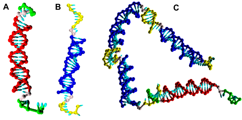
Figure 1: Cartoons of particles of (a) species $A$-and (b) species $B$, made up of a core of double-stranded DNA and two identical single strands at the ends acting as bonding sites. On both particles species, two extra bases (adenine, coloured light pink) on each side of the core have been included to decouple the free ends from the core. (c) A chain of four particles, one of species $A$ and three of species $B$. This $BBBA$ chain is composed of on4 $BB$ block of length 2 and one $AB$ block of length 1.

No condition is set on their hybridisation entropies. The nearest-neighbour model of SantaLucia santalucia1998unified allows us to compute these quantities for any given sequence: the values of $\Delta H$ and $\Delta S$ can be assumed to be temperature-independent at least in a ‘narrow’ range around $T=$310\text{\,}\mathrm{K}$$. In order to fulfil conditions (37), $B$ is chosen to be the same as $A$ with an extra pair of complementary nucleotides, one at each end, so that $B$ will bind to $B$ with greater energy than $A$ to $A$, but will still be able to bind to $A$ with roughly the same energy as $A$ to $A$. The dangling ends in an $AB$ bond will actually provide an extra contribution, usually increasing stability of $AB$ with respect to $AA$, as evaluated in bommarito2000thermodynamic ; without this stabilizing mechanism there would be no reason for $A$ and $B$ to form this mixed complex instead of only $AA$ and $BB$. This also implies that the condition $\frac{\Delta H_{AB}}{\Delta H_{AA}}\simeq 1$ is not really attainable, so we should just look for this ratio to be as close as possible to unity. Two sequences that come close to these target values are $A$=CGATCG and $B$=TCGATCGA, whose hybridisation enthalpies and entropies are reported in Table 1. Note that $A$ can bind to $A$ (being ‘palindromic’) with six bases, $B$ can bind to $B$ with eight bases, and $A$ can bind to $B$ with six bases. A cartoon of a particle is shown in figure 1.

IV Results

We ran constant-volume molecular dynamics (MD) simulations starting with $N_{A}=N_{B}=200$ bifunctional particles of types $a{\bf X}a$ and $b{\bf X}b$, for a total of 800 sticky ends on 400 particles. The resulting concentration of single strands of each species in solution is $c\approx 392\,\mu{\rm M}$. We mimicked (recall there is no explicit solvent) an aqueous solution of salt concentration $[\ce{Na+}]=$0.4\text{\,}\mathrm{M}$$, at temperatures in the range $[40,58]$\mathrm{\SIUnitSymbolCelsius}$$, where binding is expected to take place and equilibration can be achieved with the available computational resources.

From the simulation, we estimate the number of $A$ patches unbonded, bonded with $A$ ($N_{AA}$) and bonded with $B$ ($N_{AB}$). Similar quantities are calculated for $B$ patches. Using the relations previously introduced we can then estimate $p_{AA}\equiv N_{AA}/N_{A}$, $p_{BB}\equiv N_{BB}/N_{B}$ and $p_{AB}\equiv\frac{N_{AB}}{N_{A}}$, as well as $X_{A}$ and $X_{B}$.

The resulting probabilities are shown in figure 2 as symbols; the curves are the theory predictions computed as explained below. The most difficult part of the simulation is to ‘equilibrate’ the $BB$ bonds, which, being composed of more bases, are stronger and rarely break. The next-stronger bonds are $AB$ and $AA$, respectively. However, since forming $AB$ bonds would decrease the number of $BB$ bonds, the system as a whole prefers to form more $AA$ bonds than $AB$ bonds, in order to free $B$ patches for the most favourable $BB$ bonds.

From $p_{AA}$, $p_{BB}$ and $p_{AB}$ we can then predict the chain length distribution $P(n)$, where $n$ is the number of particles in the chain. Let $s$ be a sequence of bonded monomers ($A$ or $B$ particles); the probability of observing that sequence is

$$P(s)=\quantity(1-p_{A})^{m_{\overline{A}}}\quantity(1-p_{B})^{m_{\overline{B}}}p_{AB}^{n_{AB}}p_{BA}^{n_{BA}}p_{AA}^{n_{AA}}p_{BB}^{n_{BB}},$$ (38)

where $m_{\overline{\alpha}}$ is the number of free ends of type $\alpha$ and $n_{\alpha\beta}$ is the number of sites of type $\alpha$ bonded to sites of type $\beta$ (with the constraints $m_{\overline{A}}+m_{\overline{B}}=2$, $n_{AA}+n_{AB}+n_{BB}=n-1$). Then the probability $P(n)$ of observing a cluster (literally a linear chain) of length $n$) is found by summing $P(s)$ over all possible sequences of $n$ monomers:

$$P(n)=\sum_{s=1}^{2^{n}}P(s).$$ (39)

Figure 3 compares theoretical predictions and simulation data for the chain length distribution at all temperatures studied.

To evaluate $\Delta G_{\alpha\beta}$ we first combine equations (1), (27)–(29) and (34) to obtain, for $x_{A}=x_{B}=0.5$,

$$p_{\alpha\beta}=X_{\alpha}X_{\beta}\exp\left(-\beta\Delta G_{\alpha\beta}\right).$$ (40)

Equations (40) can now be solved using the data in figure 2, at each $T$. Results are plotted in figure 4. In all cases, a linear dependence of $\Delta G_{\alpha\beta}$ on $T$ is observed. The slope and intercept provide the best-fit values for $\Delta H_{\alpha\beta}$ and $\Delta S_{\alpha\beta}$, which can then be used backwards to predict the bond probabilities. These predictions are shown as solid lines in figure 2.

Table 2 compares the best-fit values of $\Delta H_{\alpha\beta}$ and $\Delta S_{\alpha\beta}$ with the predictions of the SantaLucia model. Though not excellent, agreement is reasonable, considering that the oxDNA model is a parametrisation based on SantaLucia estimates for the melting temperature. Specifically, oxDNA predictions for the melting temperatures have been found to deviate on average $1.4\text{\,}\mathrm{\SIUnitSymbolCelsius}$ from those of SantaLucia Sulc:2012 .

Finally, figure 5 plots the mean block lengths $\langle\ell_{\alpha\beta}\rangle$, vs either temperature (figure 5a) or bond probability $p_{\alpha\beta}$ (figure 5b). For our choice of parameters, both $AA$ and $AB$ blocks are very short and the simulation data are very noisy; agreement between theory and simulation is encouraging for the longer $BB$ blocks.

V Conclusions

We have proposed a minimal theoretical framework for the assembly of linear block copolymers. This makes very few assumptions on the nature of the monomers, namely: (i) assembly is assimilated to reversible chemical reactions between short-ranged bonding sites; (ii) each site can participate in at most one bond; and (iii) the overall concentration is low enough that sites and bonds behave as ideal gases. The theory requires as inputs the reaction constants for the polymerisation reactions. Importantly, these can be derived from theories that incorporate only very limited detail of the actual molecular processes.

The theory was tested against simulation results for the assembly of DNA chains from two types of short duplexes, as described by the oxDNA model, using reaction constants calculated from Santalucia’s theory of a lattice model of DNA. This was found to reproduce the equilibrium block size distributions, mean block sizes, and fractions of unreacted monomers fairly well.

The theory is easily generalised to any number of associating particle species in any proportion. In our view it has the potential to become a useful tool to predict or reverse-engineer the architectures of multi-block copolymers or polycolloids, and even provide some insight into the kinetics of association.

Conflicts of interest

There are no conflicts to declare.

$A$	$B$	$\frac{\Delta H_{BB}}{\Delta H_{AA}}$	$\frac{\Delta H_{AB}}{\Delta H_{AA}}$	$\frac{\Delta S_{BB}}{\Delta S_{AA}}$	$\frac{\Delta S_{AB}}{\Delta S_{AA}}$
CGATCG	TCGATCGA	1.27	1.09	1.24	1.09

Table 1: Relative hybridisation enthalpies and entropies of DNA single strands used in our simulations, calculated according to santalucia1998unified and bommarito2000thermodynamic .

	$AA$	$BB$	$AB$
SantaLucia
$\Delta S$ (J/mol/K)	$-126.2$	$-156.8$	$-137.1$
$\Delta H$ (kJ/mol)	$-44.6$	$-56.6$	$-48.6$
Simulation
$\Delta S$ (J/mol/K)	$-146.8$	$-166.4$	$-151.5$
$\Delta H$ (kJ/mol)	$-50.2$	$-58.8$	$-52.3$

Table 2: Comparison of best-fit values of $\Delta H_{\alpha\beta}$ and $\Delta S_{\alpha\beta}$ with the predictions of the SantaLucia model.

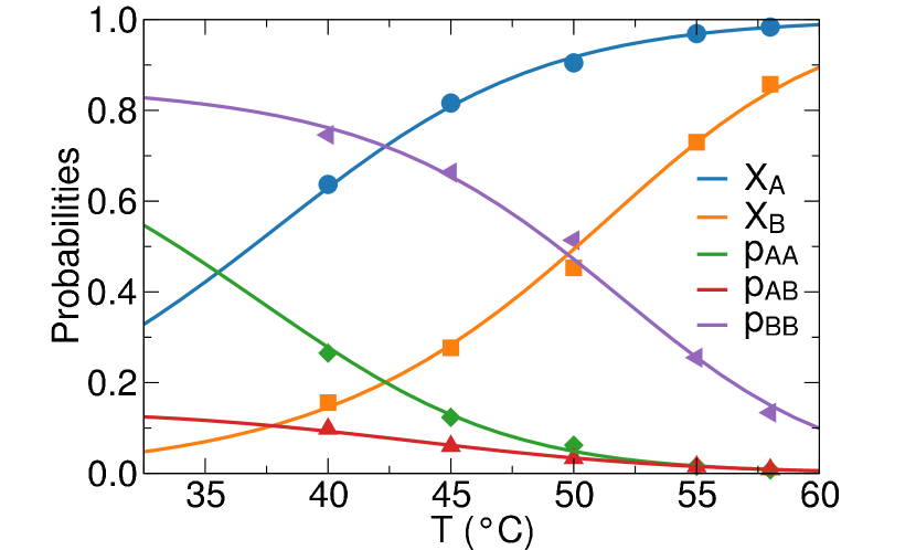
Figure 2: Probabilities $p_{AA},p_{AB}=p_{BA}$ and $p_{BB}$ of the different types of bonds between patches, and probability $X_{A}$ ($X_{B})$ that a $A$ ($B$) site is unbonded, vs temperature, from simulations (symbols) and theory (solid lines). The solid lines were obtained by solving equations (40) numerically using $\Delta H_{ij}$ and $\Delta S_{ij}$ in table 2

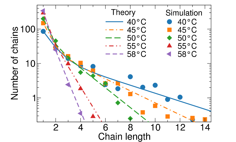
Figure 3: Comparison between expected and simulated chain length distributions at all temperatures studied.

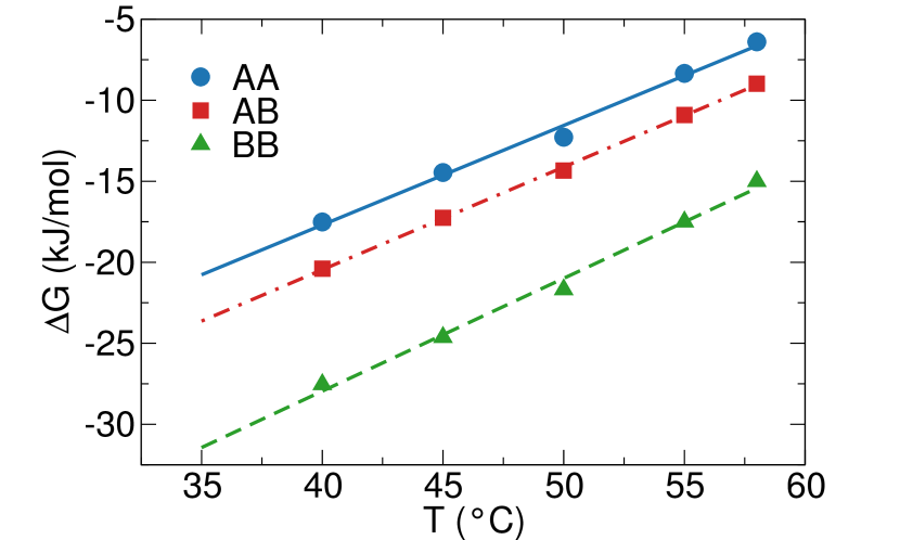
Figure 4: Binding free energy of the three complexes $AA$, $BB$ and $AB$. Symbols are the $\Delta G_{\alpha\beta}$ values obtained by solving equation (40) using the $p_{\alpha,\beta}$ from simulation. Solid lines are the linear fits $\Delta G_{\alpha\beta}=\Delta H_{\alpha\beta}-T\Delta S_{\alpha\beta}$, where $\Delta H_{\alpha\beta}$ and $\Delta S_{\alpha\beta}$ are taken as temperature-independent fit parameters (values reported in table 2).

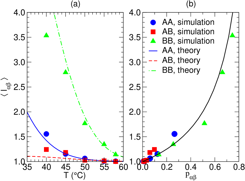
Figure 5: Mean block lengths $\langle\ell_{\alpha\beta}\rangle$ vs (a) temperature; (b) bond probability $p_{\alpha\beta}$. In (b) the black solid line is the theory prediction $1/(1-p_{\alpha\beta})$ for all block types, e.g., equations (18)–(20) when $p_{AB}=p_{BA}$