Explainable Deep Reinforcement Learning for Portfolio Management: An Empirical Approach

Abstract.

Deep reinforcement learning (DRL) has been widely studied in the portfolio management task. However, it is challenging to understand a DRL-based trading strategy because of the black-box nature of deep neural networks. In this paper, we propose an empirical approach to explain the strategies of DRL agents for the portfolio management task. First, we use a linear model in hindsight as the reference model, which finds the best portfolio weights by assuming knowing actual stock returns in foresight. In particular, we use the coefficients of a linear model in hindsight as the reference feature weights. Secondly, for DRL agents, we use integrated gradients to define the feature weights, which are the coefficients between reward and features under a linear regression model. Thirdly, we study the prediction power in two cases, single-step prediction and multi-step prediction. In particular, we quantify the prediction power by calculating the linear correlations between the feature weights of a DRL agent and the reference feature weights, and similarly for machine learning methods. Finally, we evaluate a portfolio management task on Dow Jones 30 constituent stocks during 01/01/2009 to 09/01/2021. Our approach empirically reveals that a DRL agent exhibits a stronger multi-step prediction power than machine learning methods.

1. Introduction

The explanation (Jaeger et al., 2020) of a portfolio management strategy is important to investment banks, asset management companies and hedge funds. It helps traders understand the potential risk of a certain strategy. However, it is challenging to explain a DRL-based portfolio management strategy due to the black-box nature of deep neural networks.

Existing DRL-based portfolio management works focus on enhancing the performance. A typical DRL approach of portfolio management consists of three steps as described in (Liu et al., 2020; Liu et al., 2021c; Liu et al., 2021b, a; Li et al., 2021). First, select a pool of possibly risky assets. Secondly, specify the state space, action space and reward function of the DRL agent. Finally, train a DRL agent to learn a portfolio management strategy. Such a practical approach, however, does not provide explanation to the portfolio management strategy.

In recent years, explainable deep reinforcement learning methods have been widely studied. Quantifying how much a change in input would influence the output is important to understand what contributes to the decision-making processes of the DRL agents. Thus, saliency maps (Tjoa and Guan, 2020) are adopted to provide explanation. However, these approaches are mainly available in computer vision, natural language processing and games (Atrey et al., 2019; Heuillet et al., 2021; Madumal et al., 2020). They have not been widely applied in financial applications yet. Some researchers (Cong et al., 2021) explain the DRL based portfolio management strategy using an attention model. However, it does not explain the decision-making process of a DRL agent in a proper financial context.

In this paper, we take an empirical approach to explain the portfolio management strategy of DRL agents. Our contributions are summarized as follows

• We propose a novel empirical approach to understand the strategies of DRL agents for the portfolio management task. In particular, we use the coefficients of a linear model in hindsight as the reference feature weights.

• For a deep reinforcement learning strategy, we use integrated gradients to define the feature weights, which are the coefficients between the reward and features under a linear regression model.

• We quantify the prediction power by calculating the linear correlations between the feature weights of a DRL agent and the reference feature weights, and similarly for conventional machine learning methods. Moreover, we consider both the single-step case and multiple-step case.

• We evaluate our approach on a portfolio management task with Dow Jones 30 constituent stocks during 01/01/2009 to 09/01/2021. Our approach empirically explains that a DRL agent achieves better trading performance because of its stronger multi-step prediction power.

The remainder of this paper is organized as follows. In Section 2, we review existing works on the explainable deep reinforcement learning. In Section 3, we describe the problem formulation of a DRL-based portfolio management task. In Section 4, we present the proposed explanation method. In Section 5, we show quantitative experimental results of our empirical approach. Finally, the conclusion and future work are given in Section 6.

2. Related Works

Gradient based explanation methods are widely adopted in the saliency maps (Tjoa and Guan, 2020), which quantify how much a change in input would influence the output. We review the related works of gradient based explanation for deep reinforcement learning.

• Gradient $\odot$ Input (Shrikumar et al., 2017) is the element-wise product of the gradient and the input. It provides explanation by visualizing the product as heatmap.

• Integrated Gradient (IG) (Sundararajan et al., 2017). It integrates the gradient of the output with respect to input features. For an input $\bm{x}\in\mathbb{R}^{n}$, the $i$-th entry of integrated gradient is defined as

  (1) $$\text{IG}(\bm{x})_{i}\triangleq(\bm{x}_{i}-\bm{x}^{\prime}_{i})\times\int_{z=0}^{1}\frac{\partial F(\bm{x}^{\prime}+z\cdot(\bm{x}-\bm{x}^{\prime}))}{\partial\bm{x}_{i}}dz,$$

  where $F(\cdot)$ denotes a DRL model, $\bm{x}^{\prime}$ is a perturbed version of $\bm{x}$, say replacing all entries with zeros. It explains the relationship between a model’s predictions in terms of its features.

• Guided Backpropagation (GBP) computes the gradient of the target output with respect to the input (Springenberg et al., 2015; Zeiler and Fergus, 2014), and it treats negative gradients as zeros. It provides explanation by visualizing the gradients.

• Guided GradCAM (Selvaraju et al., 2016). It uses the class-specific gradient and the final layer of a convolutional neural network to produce a coarse localization map of the important regions in an image. It provides explanation using a gradient-weighted map.

• SmoothGrad (SG) (Smilkov et al., 2017; Sundararajan et al., 2017). It creates noisy copies of an input image then averages gradients with respect to these copies. It provides explanation using visual map to identify pixels that strongly influence the final result.

Although these gradient based explanation methods are popular, they have not been directly applicable to the portfolio management task yet. Other researchers (Cong et al., 2021) explain the DRL based portfolio management using an attention model. However, it does not explain the decision-making process of DRL agent in a proper financial context.

3. Portfolio Management Using Deep Reinforcement Learning

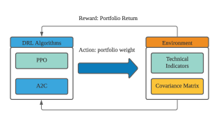
Figure 1. Overview of a portfolio management task that uses deep reinforcement learning.

We first describe a portfolio management task using a DRL agent. Then we define the feature weights using integrated gradients.

3.1. Portfolio Management Task

Consider a portfolio with $N$ risky assets over $T$ time slots, the portfolio management task aims to maximize profit and minimize risk. Let $\bm{p}(t)\in\mathbb{R}^{N}$ denotes the closing prices of all assets at time slot $t=1,...,T$. The price relative vector $\bm{y}(t)\in\mathbb{R}^{N}$ is defined as the element-wise division of $\bm{p}(t)$ by $\bm{p}(t-1)$:

(2) $$\bm{y}(t)\triangleq\left[\frac{\bm{p}_{1}(t)}{\bm{p}_{1}(t-1)},\frac{\bm{p}_{2}(t)}{\bm{p}_{2}(t-1)},...,\frac{\bm{p}_{N}(t)}{\bm{p}_{N}(t-1)}\right]^{\top},~{}~{}t=1,....T,$$

where $\bm{p}(0)\in\mathbb{R}^{N}$ is the vector of opening prices at $t=1$.

Let $\bm{w}(t)\in\mathbb{R}^{N}$ denotes the portfolio weights, which is updated at the beginning of time slot $t$. Let $v(t)\in\mathbb{R}$ denotes the portfolio value at the beginning of time slot $t+1$. Ignoring the transaction cost, we have the relative portfolio value as the ratio between the portfolio value at the ending of time slot $t$ and that at the beginning of time slot $t$,

(3) $$\frac{v(t)}{v(t-1)}=\bm{w}(t)^{\top}\bm{y}(t),$$

where $v(0)$ is the initial capital. The rate of portfolio return is

(4) $$\rho(t)\triangleq\frac{v(t)}{v(t-1)}-1=\bm{w}(t)^{\top}\bm{y}(t)-1,$$

while correspondingly the logarithmic rate of portfolio return is

(5) $$r(t)\triangleq\ln\frac{v(t)}{v(t-1)}=\ln(\bm{w}(t)^{\top}\bm{y}(t)).$$

The risk of a portfolio is defined as the variance of the rate of portfolio return $\rho(t)$:

(6) $$\begin{split}&\text{Risk}(t)\triangleq\text{Var}(\rho(t))=\text{Var}(\bm{w}(t)^{\top}\bm{y}(t)-1)\\ &=\text{Var}(\bm{w}(t)^{\top}\bm{y}(t))=\bm{w}(t)^{\top}~{}\text{Cov}(\bm{y}(t))~{}\bm{w}(t)\\ &=\bm{w}(t)^{\top}~{}\bm{\Sigma}(t)~{}\bm{w}(t),\end{split}$$

where $\bm{\Sigma}(t)=\text{Cov}(\bm{y}(t))\in\mathbb{R}^{N\times N}$ is the covariance matrix of the stock returns at the end of time slot $t$. If there is no transaction cost, the final portfolio value is

(7) $$v(T)=v(0)~{}\exp\left(\sum\limits_{t=1}^{T}r(t)\right)=v(0)~{}\prod\limits_{t=1}^{T}\bm{w}(t)^{\top}\bm{y}(t).$$

The portfolio management task (Boyd et al., 2017; Wikipedia contributors, 2021c) aims to find a portfolio weight vector $\bm{w}^{*}(t)\in\mathbb{R}^{N}$ such that

(8) $$\begin{split}\bm{w}^{*}(t)\triangleq&\text{argmax}_{\bm{w}(t)}~{}~{}~{}~{}\bm{w}^{\top}(t)~{}\bm{y}(t)-\lambda~{}\bm{w}^{\top}(t)~{}\bm{{\Sigma}}(t)~{}\bm{w}(t),\\ &\text{s.t.}~{}~{}~{}\sum_{i=1}^{N}\bm{w}_{i}(t)=1,~{}~{}~{}~{}\bm{w}_{i}(t)\in[0,1],~{}~{}~{}~{}~{}~{}t=1,...,T\end{split}$$

where $\lambda>0$ is the risk aversion parameter. Since $\bm{y}(t)$ and $\bm{\Sigma}(t)$ are revealed at the end of time slot $t$. We estimate them at the the beginning of time slot $t$.

We use $\widehat{\bm{y}}(t)\in\mathbb{R}^{N}$ to estimate the price relative vector $\bm{y}(t)$ in (8) by applying a regression model on predictive financial features (Feng et al., 2017) based on Capital Asset Pricing Model (CAPM) (Fama and French, 2004). We use $\widehat{\bm{\Sigma}}(t)$, the sample covariance matrix, to estimate covariance matrix $\bm{\Sigma}(t)$ in (8) using historical data.

Then, at the beginning of time slot $t$, our goal is to find optimal portfolio weights

(9) $$\begin{split}\bm{w}^{*}(t)\triangleq&\text{argmax}_{\bm{w}(t)}~{}~{}~{}~{}\bm{w}^{\top}(t)~{}\widehat{\bm{y}}(t)-\lambda~{}\bm{w}^{\top}(t)~{}\widehat{\bm{{\Sigma}}}(t)~{}\bm{w}(t),\\ &\text{s.t.}~{}~{}~{}\sum_{i=1}^{N}\bm{w}_{i}(t)=1,~{}~{}~{}~{}\bm{w}_{i}(t)\in[0,1],~{}~{}~{}~{}~{}~{}t=1,...,T.\end{split}$$

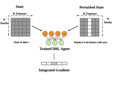
Figure 2. Feature weights of a trained DRL agent.

3.2. Deep Reinforcement Learning for Portfolio Management

We describe how to use deep reinforcement learning algorithms for the portfolio management task, by specifying the state space, action space and reward function. We use a similar setting as in the open-source FinRL library (Liu et al., 2020)(Liu et al., 2021c).

State space $\mathcal{S}$ describes an agent’s perception of a market. The state at the beginning of time slot $t$ is

(10) $$\bm{s}(t)=[\bm{f}^{1}(t),...,\bm{f}^{K}(t),\widehat{\bm{\Sigma}}(t)]\in\mathbb{R}^{N\times(N+K)},~{}~{}~{}~{}~{}~{}t=1,...,T,$$

where $\bm{f}^{k}(t)\in\mathbb{R}^{N}$ denotes the vector for the $k$-th feature at the beginning of time slot $t$.

Action space $\mathcal{A}$ describes the allowed actions an agent can take at a state. In our task, the action $\bm{w}(t)\in\mathbb{R}^{N}$ corresponds to the portfolio weight vector decided at the beginning of time slot $t$ and should satisfy the constraints in (9). We use a softmax layer as the last layer to meet the constraints.

Reward function. The reward function $r(\bm{s}(t),\bm{w}(t),\bm{s}(t+1))$ is the incentive for an agent to learn a profitable policy. We use the logarithmic rate of portfolio return in (5) as the reward,

(11) $$r(\bm{s}(t),\bm{w}(t),\bm{s}(t+1))=\ln(\bm{w}^{\top}(t)\cdot\bm{y}(t)).$$

The agent takes $\bm{s}(t)$ as input at the beginning of time slot $t$ and output $\bm{w}(t)$ as the portfolio weight vector.

DRL algorithms. We use two popular deep reinforcement learning algorithms: Advantage Actor Critic (A2C) (Mnih et al., 2016) and Proximal Policy Optimization (PPO) (Schulman et al., 2017). A2C (Mnih et al., 2016) utilizes an advantage function to reduce the variance of the policy gradient. Its objective function is

(12) $$\triangledown J_{\theta}(\theta)=\mathbb{E}\left[\sum_{t=1}^{T}\triangledown_{\theta}\log\pi_{\theta}(\bm{w}(t)|\bm{s}(t))A(\bm{s}(t),\bm{w}(t))\right],$$

where $\pi_{\theta}(\bm{w}(t)|\bm{s}(t))$ is the policy network parameterized by $\theta$ and $A(\bm{s}(t),\bm{w}(t))$ is an advantage function defined as follows

(13) $$\begin{split}&A(\bm{s}(t),\bm{w}(t))=Q(\bm{s}(t),\bm{w}(t))-V(\bm{s}(t))\\ &=r(\bm{s}(t),\bm{w}(t),\bm{s}(t+1))+\gamma V(\bm{s}(t+1))-V(\bm{s}(t)),\end{split}$$

where $Q(\bm{s}(t),\bm{w}(t))$ is the expected reward at state $\bm{s}(t)$ when taking action $\bm{w}(t)$, $V(\bm{s}(t))$ is the value function, $\gamma\in(0,1]$ is a discount factor. PPO (Schulman et al., 2017) is used to control the policy gradient update and to ensure that the new policy will be close to the previous one. It uses a surrogate objective function

(14) $$\begin{split}&J^{\text{CLIP}}(\theta)=\\ &\mathbb{E}(t)[\text{min}(R_{t}(\theta)\widehat{A}(\bm{s}(t),\bm{w}(t)),\text{clip}(R_{t}(\theta),1-\epsilon,1+\epsilon)~{}\widehat{A}(\bm{s}(t),\bm{w}(t))],\end{split}$$

where $R_{t}(\theta)\triangleq\frac{\pi_{\theta}(\bm{w}(t)|\bm{s}(t))}{\pi_{\theta_{old}}(\bm{w}(t)|\bm{s}(t))}$ is the probability ratio between new and old policies, $\widehat{A}(\bm{s}(t),\bm{w}(t))$ is the estimated advantage function, and the clip function $\text{clip}(R_{t}(\theta),1-\epsilon,1+\epsilon)$ truncates the ratio $R_{t}(\theta)$ to be within the range $[1-\epsilon,1+\epsilon]$.

3.3. Feature Weights Using Integrated Gradients

We use the integrated gradients in (1) to measure the feature weights (Sundararajan et al., 2017; Tomsett et al., 2020). For a trained DRL agent, the integrated gradient (Sundararajan et al., 2017) under policy $\pi$ for the $k$-th feature of the $i$-th asset is defined as

(15) $$\begin{split}&IG(\bm{f}^{k}(t))_{i}\\ &=(\bm{f}^{k}(t)_{i}-\bm{f}^{k^{\prime}}(t)_{i})\\ &\times\int_{z=0}^{1}\frac{\partial Q^{\pi}(\bm{s}_{k}^{\prime}(t)+z\cdot(\bm{s}(t)-\bm{s}_{k}^{\prime}(t)),\bm{w}(t))}{\partial\bm{f}^{k}(t)_{i}}dz\\ &=\bm{f}^{k}(t)_{i}\cdot\frac{\partial Q^{\pi}(\bm{s}_{k}^{\prime}(t)+z^{k,i}\cdot(\bm{s}(t)-\bm{s}_{k}^{\prime}(t)),\bm{w}(t))}{\partial\bm{f}^{k}(t)_{i}}\cdot(1-0)\\ &=\bm{f}^{k}(t)_{i}\\ &\cdot\frac{\partial\mathbb{E}\left[\sum_{l=0}^{\infty}\gamma^{l}\cdot r(\bm{s}^{k,i}(t+l),\bm{w}(t+l),\bm{s}^{k,i}(t+l+1))|\bm{s}^{k,i}(t),\bm{w}(t)\right]}{\partial\bm{f}^{k}(t)_{i}}\\ &=\bm{f}^{k}(t)_{i}\cdot\sum_{l=0}^{\infty}\gamma^{l}\cdot\frac{\partial\mathbb{E}\left[\ln(\bm{w}^{\top}(t+l)\cdot\bm{y}(t+l))|\bm{s}^{k,i}(t),\bm{w}(t)\right]}{\partial\bm{f}^{k}(t)_{i}}\\ &\approx\bm{f}^{k}(t)_{i}\cdot\sum_{l=0}^{\infty}\gamma^{l}\cdot\frac{\partial\mathbb{E}\left[\bm{w}^{\top}(t+l)\cdot\bm{y}(t+l)-1|\bm{s}^{k,i}(t),\bm{w}(t)\right]}{\partial\bm{f}^{k}(t)_{i}}\\ &=\bm{f}^{k}(t)_{i}\cdot\sum_{l=0}^{\infty}\gamma^{l}\cdot\frac{\partial\mathbb{E}\left[\bm{w}^{\top}(t+l)\cdot\bm{y}(t+l)|\bm{s}^{k,i}(t),\bm{w}(t)\right]}{\partial\bm{f}^{k}(t)_{i}},\end{split}$$

where the first equality holds by definition in (1), the second equality holds because of the mean value theorem (Wikipedia contributors, 2021b), the third equality holds because

(16) $$Q^{\pi}(\bm{s}(t),\bm{w}(t))\triangleq\mathbb{E}\left[\sum_{l=0}^{\infty}\gamma^{l}\cdot r(\bm{s}(t+l),\bm{w}(t+l),\bm{s}(t+l+1))|\bm{s}(t),\bm{w}(t)\right],$$

the approximation holds because $\ln(\bm{w}^{\top}(t)\cdot\bm{y}(t))\approx\bm{w}^{\top}(t)\cdot\bm{y}(t)-1$ when $\bm{w}^{\top}(t)\cdot\bm{y}(t)$ is close to 1. $\bm{s}_{k}^{\prime}(t)\in\mathbb{R}^{N\times(N+K)}$ is a perturbed version of $\bm{s}(t)$ by replacing the $k$-th feature with an all-zero vector. $\bm{s}^{k,i}(t)$ is a linear combination of original state and perturbed state $\bm{s}^{k,i}(t)\triangleq\bm{s}_{k}^{\prime}(t)+z^{k,i}\cdot(\bm{s}(t)-\bm{s}_{k}^{\prime}(t))$, where $z^{k,i}\in[0,1]$.

4. Explanation Method

We propose an empirical approach to explain the portfolio management task that uses a trained DRL agent.

4.1. Overview of Our Empirical Approach

Our empirical approach consists of three parts.

• First, we study the portfolio management strategy using feature weights, which quantify the relationship between the reward (say, portfolio return) and the input (say, features). In particular, we use the coefficients of a linear model in hindsight as the reference feature weights.

• Then, for the deep reinforcement learning strategy, we use integrated gradients to define the feature weights, which are the coefficients between reward and features under a linear regression model

• Finally, we quantify the prediction power by calculating the linear correlations between the coefficients of a DRL agent and the reference feature weights, and similarly for conventional machine learning methods. Moreover, we consider both the single-step case andmultiple-step case.

4.2. Reference Feature Weights

For the portfolio management task, we use a linear model in hindsight as a reference model. For a linear model in hindsight, a demeon would optimize the portfolio (Brown et al., 2020) with actual stock returns and the actual sample covariance matrix. It is the upper bound performance that any linear predictive model would have been able to achieve.

The portfolio value relative vector is the element-wise product of weight and price relative vectors, $\bm{q}(t)\triangleq\bm{w}(t)$ $\odot$ $\bm{y}(t)\in\mathbb{R}^{N}$, where $\bm{w}(t)$ is the optimal portfolio weight. We represent it as a linear regression model as follows

(17) $$\bm{q}(t)=\beta_{0}(t)\cdot[1,...,1]^{\top}+\beta_{1}(t)\cdot\bm{f}^{1}(t)+...+\beta_{K}(t)\cdot\bm{f}^{K}(t)+\bm{\epsilon}(t),$$

where $\beta_{k}(t)\in\mathbb{R}$ is regression coefficient of the $k$-th feature. $\bm{\epsilon}(t)\in\mathbb{R}^{N}$ is the error vector, where the elements are assumed to be independent and normally distributed.

We define the reference feature weights as

$\bm{\beta}(t)\triangleq\left[\bm{\beta}(t)_{1},\bm{\beta}(t)_{2},...\bm{\beta}(t)_{K}\right]^{\top}\in\mathbb{R}^{K}$, where

(18) $$\bm{\beta}(t)_{k}=\sum_{i=1}^{N}\beta_{k}(t)\cdot\bm{f}^{k}(t)_{i},$$

is the inner product of $\frac{\partial(\bm{q}^{\top}(t)\cdot\bm{1})}{\partial\bm{f}^{k}(t)}=\beta_{k}(t)\cdot[1,...,1]^{\top}$ and $\bm{f}^{k}(t)$ that characterizes the total contribution of the $k$-th feature to the portfolio value at time $t$.

4.3. Feature Weights for DRL Trading Agent

For a DRL agent in portfolio management task, at the beginning of a trading slot $t$, it takes the feature vectors and co-variance matrix as input. Then it outputs an action vector, which is the portfolio weight vector $\bm{w}(t)$. We also represent it as a linear regression model,

(19) $$\bm{q}(t)=c_{0}(t)\cdot[1,...,1]^{\top}+c_{1}(t)\cdot\bm{f}^{1}(t)+...+c_{K}(t)\cdot\bm{f}^{K}(t)+\bm{\epsilon}(t).$$

As Fig. 2 shows, for the decision-making process of a DRL agent, we define the feature weights for the $k$-th feature as

(20) $$\begin{split}&\bm{M}^{\pi}(t)_{k}\triangleq\sum_{i=1}^{N}IG(\bm{f}^{k}(t))_{i}\\ &\approx\sum_{i=1}^{N}\bm{f}^{k}(t)_{i}\cdot\sum_{l=0}^{\infty}\gamma^{l}\cdot\frac{\partial\mathbb{E}\left[\bm{w}^{\top}(t+l)\cdot\bm{y}(t+l))|\bm{s}^{k,i}(t),\bm{w}(t)\right]}{\partial\bm{f}^{k}(t)_{i}}\\ &=\sum_{i=1}^{N}\bm{f}^{k}(t)_{i}\cdot\sum_{l=0}^{\infty}\gamma^{l}\cdot\mathbb{E}\left[c_{k}(t+l)\frac{\partial\bm{f}^{k}(t+l)_{i}}{\partial\bm{f}^{k}(t)_{i}}|\bm{s}^{k,i}(t),\bm{w}(t)\right],\end{split}$$

where the last equality holds due to the fact that $\frac{\partial\bm{w}^{\top}(t+l)\cdot\bm{y}(t+l)}{\partial\bm{f}^{k}(t)_{i}}$ is continuous and $\bm{w}^{\top}(t+l)\cdot\bm{y}(t+l)$ is bounded for any $t$ (Wikipedia contributors, 2021a, b).

Assuming the time dependency of features on stocks follows the power law, i.e., $\frac{\partial\bm{f}^{k}(t+l)_{i}}{\partial\bm{f}^{k}(t)_{i}}=l^{-\alpha}$, where $\alpha\in\mathbb{R}^{+}$, for $l\geq 1$, then the feature weights are

(21) $$\begin{split}&\bm{M}^{\pi}(t)_{k}\\ &=\sum_{i=1}^{N}\bm{f}^{k}(t)_{i}\cdot\sum_{l=0}^{\infty}\gamma^{l}\cdot\mathbb{E}\left[c_{k}(t+l)\frac{\partial\bm{f}^{k}(t+l)_{i}}{\partial\bm{f}^{k}(t)_{i}}|\bm{s}^{k,i}(t),\bm{w}(t)\right]\\ &=\sum_{i=1}^{N}\bm{f}^{k}(t)_{i}\cdot\\ &\{\mathbb{E}\left[c_{k}(t)|\bm{s}^{k,i}(t),\bm{w}(t)\right]+\sum_{l=1}^{\infty}\gamma^{l}\cdot\mathbb{E}\left[c_{k}(t+l)\cdot l^{-\alpha}|\bm{s}^{k,i}(t),\bm{w}(t)\right]\}\\ &=\sum_{i=1}^{N}\bm{f}^{k}(t)_{i}\cdot\mathbb{E}\left[c_{k}(t)+\sum_{l=1}^{\infty}\gamma^{l}\cdot l^{-\alpha}\cdot c_{k}(t+l)|\bm{s}^{k,i}(t),\bm{w}(t)\right].\end{split}$$

Notice that $\bm{M}^{\pi}(t)_{k}$ has a similar form as $\bm{\beta}(t)_{k}$ in (18). The $\beta_{k}(t)$ are replaced by $\mathbb{E}\left[c_{k}(t)+\sum_{l=1}^{\infty}\gamma^{l}\cdot l^{-\alpha}\cdot c_{k}(t+l)|\bm{s}^{k,i}(t),\bm{w}(t)\right]$ in the context of a DRL agent. This better characterizes the superiority of the DRL agents to maximize future rewards.

4.4. Quantitative Comparison

Our empirical approach provides explanations by quantitatively comparing the feature weights to the reference feature weights.
Conventional Machine Learning Methods with Forward-Pass
A conventional machine learning method with a forward-pass has three steps: 1) Predict stock returns with machine learning methods using features. 2) Find optimal portfolio weights under predicted stock returns. 3) Build a regression model between portfolio return and features.

(22) $$\begin{split}\widehat{\bm{y}}(t)&=g(\bm{f}^{1}(t),...,\bm{f}^{K}(t)),\\ \bm{q}^{*}(t)&=\bm{w}^{*}(t)\odot\bm{y}(t),\\ \bm{q}^{*}(t)&=b_{0}(t)\cdot\bm{1}+b_{1}(t)\cdot\bm{f}^{1}(t)+...+b_{K}(t)\cdot\bm{f}^{K}(t)+\bm{\epsilon}(t),\\ t&=1,...,T,\end{split}$$

where $g(\cdot)$ is the machine learning regression model. $b_{k}(t)$ is the gradient of the portfolio return to the $k$-th feature at time slot $t$, $i=1,...,K$. $\bm{y}(t)$ is the true price relative vector at time $t$. $\widehat{\bm{y}}(t)$ is the predicted price relative vector at time $t$. $\bm{w}^{*}(t)$ is the optimal portfolio weight vector defined in (9), where we set the risk aversion parameter to 0.5. Likewise, we define the feature weights $\bm{b}(t)_{k}$ by

(23) $$\bm{b}(t)_{k}=\sum_{i=1}^{N}b_{k}(t)\cdot\bm{f}^{k}(t)_{i},$$

which is similar to how we define $\bm{\beta}(t)_{k}$ and $\bm{M}^{\pi}(t)_{k}$.
Linear Correlations
Both the machine learning methods and DRL agents take profits from their prediction power. We quantify the prediction power by calculating the linear correlations $\rho(\cdot)$ between the feature weights of a DRL agent and the reference feature weights and similarly for machine learning methods.

Furthermore, the machine learning methods and DRL agents are different when predicting future. The machine learning methods rely on single-step prediction to find portfolio weights. However, the DRL agents find portfolio weights with a long-term goal. Then, we compare two cases, single-step prediction and multi-step prediction.

For each time step, we compare a method’s feature weights with $\bm{\beta}(t)$ to measure the single-step prediction. For multi-step prediction, we compare wih a smoothed vector,

(24) $$\bm{\beta}^{W}(t)=\frac{\sum_{j=0}^{W-1}\bm{\beta}(t+j)}{W},$$

where $W$ is the number of time steps of interest. It is the average reference feature weights over $W$ steps.

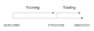
Figure 3. Data split for the training and trading periods.

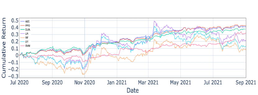
Figure 4. The cumulative portfolio return curves of machine learning and DRL models (from 2020-07-01 to 2021-09-01).

For $t=1,...,T$, we use the average values as metrics. For the machine learning methods, we measure the single-step and multi-step prediction power using

(25) $$\begin{split}\overline{\rho}(\bm{b},\bm{\beta})&=\frac{\sum_{t=1}^{T}\rho(\bm{b}(t),\bm{\beta}(t))}{T},\\ \overline{\rho}(\bm{b},\bm{\beta}^{W})&=\frac{\sum_{t=1}^{T-W+1}\rho(\bm{b}(t),\bm{\beta}^{W}(t))}{T-W+1}.\\ \end{split}$$

For the DRL-agents, we measure the single-step and multi-step prediction power using

(26) $$\begin{split}\overline{\rho}(\bm{M},\bm{\beta})&=\frac{\sum_{t=1}^{T}\rho(\bm{M}(t),\bm{\beta}(t))}{T},\\ \overline{\rho}(\bm{M},\bm{\beta}^{W})&=\frac{\sum_{t=1}^{T-W+1}\rho(\bm{M}(t),\bm{\beta}^{W}(t))}{T-W+1}.\\ \end{split}$$

In (25) and (26), the first metric represents the average single-step prediction power during the whole trading period. The second metric then measures the average multi-step prediction power.

These two metrics are important to explain the portfolio management task.

• Portfolio performance: A closer relationship to the reference model indicates a higher prediction power and therefore a better portfolio performance. Both the single-step prediction and multi-step prediction power are expected to be positively correlated to the portfolio’s performance.

• The advantage of DRL agents: The DRL agents make decisions with a long-term goal. Therefore the multi-step prediction power of DRL agents is expected to outperform their single-step prediction power.

• The advantage of machine learning methods: The portfolio management strategy with machine learning methods relies on single-step prediction power. Therefore, the single-step prediction power of machine learning methods is expected to outperform their multi-step prediction power.

• The comparison between DRL agents and machine learning methods: The DRL agents are expected to outperform the machine learning methods in multi-step prediction power and fall behind in single-step prediction power.

5. Experimental Results

In this section, we describe the data set, compared machine learning methods, trading performance and explanation analysis.

Table 1. Comparison of trading performance.

(2020/07/01-2021/09/01)	PPO	A2C	DT	LR	RF	SVM	DJIA
Annual Return	35.0%	34 %	10.8%	17.6%	6.5%	26.2%	31.2%
Annual Volatility	14.7%	14.9 %	40.1%	42.4%	41.2 %	16.2 %	14.1 %
Sharpe Ratio	2.11	2.04	0.45	0.592	0.36	1.53	2.0
Calmar Ratio	4.23	4.30	0.46	0.76	0.21	2.33	3.5
Max Drawdown	-8.3%	-7.9%	-23.5%	-23.2%	-30.7 %	-11.3 %	-8.9 %
Ave. Corr. Coeff. (single-step)	0.024	0.030	0.068	0.055	0.052	0.034	N/A
Ave. Corr. Coeff. (multi-step)	0.09	0.078	-0.03	-0.03	-0.015	-0.006	N/A

5.1. Stock Data and Feature Extraction

We describe the stock data and the features.
Stock data. We use the FinRL library (Liu et al., 2020) and the stock data of Dow Jones 30 constituent stocks, accessed at the beginning of our testing period, from 01/01/2009 to 09/01/2021. The stock data is divided into two sets. Training data set (from 01/01/2009 to 06/30/2020) is used to train the DRL agents and machine learning models, while trading data set (from 07/01/2020 to 09/01/2021) is used for back-testing the trading performance.
Features. We use four technical indicators as features in our experiments.

• MACD: Moving Average Convergence Divergence.

• RSI: Relative Strength Index.

• CCI: The Commodity Channel Index.

• ADX: Average Directional Index.

All data and features are measured in a daily time granularity.

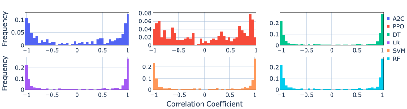
Figure 5. The histogram of correlation coefficient (single-step) for Advantage Actor Critic (A2C), Proximal Policy Optimization (PPO), Decision Tree (DT), Linear Regression (LR), Support Vector Machine (SVM) and Random Forest (RF).

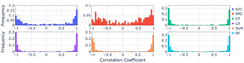
Figure 6. The histogram of correlation coefficients (multiple-step) for Advantage Actor Critic (A2C), Proximal Policy Optimization (PPO), Decision Tree (DT), Linear Regression (LR), Support Vector Machine (SVM) and Random Forest (RF).

Table 2. Upper tail test table for mean correlation coefficient (single-step and multi-step) under null hypothesis: the mean correlation coefficient is of no difference than zero.

	Z-statistics (single-step)	Z-statistics (multi-step)
PPO	0.6	$\textbf{2.16}^{***}$
A2C	0.51	$\textbf{1.58}^{**}$
DT	$\textbf{1.28}^{**}$	-0.59
LR	1.03	-0.55
RF	0.98	-0.28
SVM	0.64	-0.11

5.2. Compared Machine Learning Methods

We describe the models we use in experiment. We use four classical machine learning regression models (Pedregosa et al., 2011): Support Vector Machine (SVM), Decision Tree Regression (DT), Linear Regression (LR), Random Forest (RF) and two deep reinforcement learning models: A2C and PPO.

5.3. Performance Comparison

We use several metrics to evaluate the trading performance.

• Annual return: the geometric average portfolio return each year.

• Annual volatility: The annual standard deviation of the portfolio return.

• Maximum drawdown: The maximum percentage loss during the trading period.

• Sharpe ratio: The annualized portfolio return in excess of the risk-free rate per unit of annualized volatility.

• Calmar ratio: The average portfolio return per unit of maximum drawdown.

• Average Correlation Coefficient (single-step): It measures a model’s single-step prediction capability.

• Average Correlation Coefficient (multi-step): It measures a model’s multi-step prediction capability. We set $W=20$ in (24).

As shown in by Fig. 4 and Table 1, the DRL agent using PPO reached 35$\%$ for annual return and 2.11 for Sharpe ratio, which performed the best among all the others. The other DRL agent using A2C reached 34$\%$ for annual return and 2.04 for Sharpe ratio. Both of them performed better than the Dow Jones Industrial Average (DJIA), which reached 31.2$\%$ for annual return and 2.0 for Sharpe ratio. As for the machine learning methods, the support vector machine method reached the highest Sharpe ratio: 1.53 and the highest annual return: 26.2$\%$. None of the machine learning methods outperformed the Dow Jones Industrial Average (DJIA).

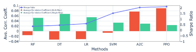
Figure 7. The comparison of Sharpe ratio and average correlation coefficient.

5.4. Explanation Analysis

We calculate the histogram of correlation coefficients with 1770 samples for 295 trading days. From Fig. 5 and Fig. 6, we visualize the the distribution of correlation coefficients. We derived the statistical tests as in Table 2, where ”**”, ”***” denote significance at the 10$\%$ and 5$\%$ level. We find that

• The distributions of correlation coefficients are different between the DRL agents and machine learning methods.

• The machine learning methods show greater significance in mean correlation coefficient (single-step) than DRL agents.

• The DRL agents show stonger significance in mean correlation coefficient (multi-step) than machine learning methods.

We show our method empirically explains the superiority of DRL agents for the portfolio management task. As Fig. 7 shows, the y-axis represents the average coefficients and Sharpe ratio for the whole trading data set, the x-axis represents the model. From Table 1 and Fig. 7, we find that

• The DRL agent using PPO has the highest Sharpe ratio:2.11 and highest average correlation coefficient (multi-step): 0.09 among all the others.

• The DRL agents’ average correlation coefficients (multi-step) are significantly higher than their average correlation coefficients (single-step).

• The machine learning methods’ average correlation coefficients (single-step) are significantly higher than their average correlation coefficients (multi-step).

• The DRL agents outperform the machine learning methods in multi-step prediction power and fall behind in single-step prediction power.

• Overall, a higher mean correlation coefficient (multi-step) indicates a higher Sharpe ratio.

6. Conclusion

In this paper, we empirically explained the DRL agents’ strategies for the portfolio management task. We used a linear model in hindsight as the reference model. We found out the relationship between the reward (namely, the portfolio return) and the input (namely, the features) using integrated gradients. We measured the prediction power using correlation coefficients.

We used Dow Jones 30 constituent stocks from 01/01/2009 to 09/01/2021 and empirically showed that DRL agents outperformed the machine learning models in multi-step prediction. For future work, we will explore the explanation methods for other deep reinforcement learning algorithms and study on other financial applications including trading, hedging and risk management.

References

- (1)
- Atrey et al. (2019) Akanksha Atrey, Kaleigh Clary, and David Jensen. 2019. Exploratory not explanatory: Counterfactual analysis of saliency maps for deep reinforcement learning. In International Conference on Learning Representations.
- Boyd et al. (2017) Stephen Boyd, Enzo Busseti, Steve Diamond, Ronald N Kahn, Kwangmoo Koh, Peter Nystrup, Jan Speth, et al. 2017. Multi-period trading via convex optimization. Foundations and Trends® in Optimization 3, 1 (2017), 1–76.
- Brown et al. (2020) Ryan Brown, Harindra de Silva, and Patrick D Neal. 2020. Portfolio performance attribution: A machine learning-based approach. Machine Learning for Asset Management: New Developments and Financial Applications (2020), 369–386.
- Cong et al. (2021) Lin William Cong, Ke Tang, Jingyuan Wang, and Yang Zhang. 2021. AlphaPortfolio: Direct construction through deep reinforcement learning and interpretable AI. Available at SSRN 3554486 (2021).
- Fama and French (2004) Eugene F Fama and Kenneth R French. 2004. The capital asset pricing model: Theory and evidence. Journal of Economic Perspectives 18, 3 (2004), 25–46.
- Feng et al. (2017) Guanhao Feng, Stefano Giglio, and Dacheng Xiu. 2017. Taming the factor zoo. Fama-Miller Working Paper 24070 (2017).
- Heuillet et al. (2021) Alexandre Heuillet, Fabien Couthouis, and Natalia Díaz-Rodríguez. 2021. Explainability in deep reinforcement learning. Knowledge-Based Systems 214 (2021), 106685.
- Jaeger et al. (2020) Markus Jaeger, Stephan Krügel, Dimitri Marinelli, Jochen Papenbrock, and Peter Schwendner. 2020. Understanding machine learning for diversified portfolio construction by explainable AI. Available at SSRN 3528616 (2020).
- Li et al. (2021) Zechu Li, Xiao-Yang Liu, Jiahao Zheng, Zhaoran Wang, Anwar Walid, and Jian Guo. 2021. FinRL-Podracer: High performance and scalable deep reinforcement learning for quantitative finance. ACM International Conference on AI in Finance (ICAIF) (2021).
- Liu et al. (2021a) Xiao-Yang Liu, Zechu Li, Zhuoran Yang, Jiahao Zheng, Zhaoran Wang, Anwar Walid, Jian Guo, and Michael Jordan. 2021a. ElegantRL-Podracer: Scalable and elastic library for cloud-native deep reinforcement learning. Deep RL Workshop, NeurIPS 2021 (2021).
- Liu et al. (2021b) Xiao-Yang Liu, Jingyang Rui, Jiechao Gao, Liuqing Yang, Hongyang Yang, Zhaoran Wang, Christina Dan Wang, and Guo Jian. 2021b. Data-driven deep reinforcement learning in quantitative finance. Data-Centric AI Workshop, NeurIPS (2021).
- Liu et al. (2020) Xiao-Yang Liu, Hongyang Yang, Qian Chen, Runjia Zhang, Liuqing Yang, Bowen Xiao, and Christina Dan Wang. 2020. FinRL: A deep reinforcement learning library for automated stock trading in quantitative finance. NeurIPS Workshop on Deep Reinforcement Learning (2020).
- Liu et al. (2021c) Xiao-Yang Liu, Hongyang Yang, Jiechao Gao, and Christina Dan Wang. 2021c. FinRL: Deep reinforcement learning framework to automate trading in quantitative finance. ACM International Conference on AI in Finance (ICAIF) (2021).
- Madumal et al. (2020) Prashan Madumal, Tim Miller, Liz Sonenberg, and Frank Vetere. 2020. Explainable reinforcement learning through a causal lens. In Proceedings of the AAAI Conference on Artificial Intelligence, Vol. 34. 2493–2500.
- Mnih et al. (2016) Volodymyr Mnih, Adria Puigdomenech Badia, Mehdi Mirza, Alex Graves, Timothy Lillicrap, Tim Harley, David Silver, and Koray Kavukcuoglu. 2016. Asynchronous methods for deep reinforcement learning. In International Conference on Machine Learning. PMLR, 1928–1937.
- Pedregosa et al. (2011) F. Pedregosa, G. Varoquaux, A. Gramfort, V. Michel, B. Thirion, O. Grisel, M. Blondel, P. Prettenhofer, R. Weiss, V. Dubourg, J. Vanderplas, A. Passos, D. Cournapeau, M. Brucher, M. Perrot, and E. Duchesnay. 2011. Scikit-learn: Machine learning in Python. Journal of Machine Learning Research 12 (2011), 2825–2830.
- Schulman et al. (2017) John Schulman, Filip Wolski, Prafulla Dhariwal, Alec Radford, and Oleg Klimov. 2017. Proximal policy optimization algorithms. arXiv preprint arXiv:1707.06347 (2017).
- Selvaraju et al. (2016) Ramprasaath R Selvaraju, Abhishek Das, Ramakrishna Vedantam, Michael Cogswell, Devi Parikh, and Dhruv Batra. 2016. Grad-CAM: Why did you say that? arXiv preprint arXiv:1611.07450 (2016).
- Shrikumar et al. (2017) Avanti Shrikumar, Peyton Greenside, and Anshul Kundaje. 2017. Learning important features through propagating activation differences. In International Conference on Machine Learning. PMLR, 3145–3153.
- Smilkov et al. (2017) Daniel Smilkov, Nikhil Thorat, Been Kim, Fernanda Viégas, and Martin Wattenberg. 2017. Smoothgrad: removing noise by adding noise. arXiv preprint arXiv:1706.03825 (2017).
- Springenberg et al. (2015) J Springenberg, Alexey Dosovitskiy, Thomas Brox, and M Riedmiller. 2015. Striving for simplicity: The all convolutional net. In ICLR (workshop track).
- Sundararajan et al. (2017) Mukund Sundararajan, Ankur Taly, and Qiqi Yan. 2017. Axiomatic attribution for deep networks. In International Conference on Machine Learning. PMLR, 3319–3328.
- Tjoa and Guan (2020) Erico Tjoa and Cuntai Guan. 2020. A survey on explainable artificial intelligence (XAI): Toward medical XAI. IEEE Transactions on Neural Networks and Learning Systems (2020).
- Tomsett et al. (2020) Richard Tomsett, Dan Harborne, Supriyo Chakraborty, Prudhvi Gurram, and Alun Preece. 2020. Sanity checks for saliency metrics. In Proceedings of the AAAI conference on artificial intelligence, Vol. 34. 6021–6029.
- Wikipedia contributors (2021a) Wikipedia contributors. 2021a. Dominated convergence theorem — Wikipedia, The Free Encyclopedia. https://en.wikipedia.org/w/index.php?title=Dominated_convergence_theorem&oldid=1037463814 [Online; accessed 17-September-2021].
- Wikipedia contributors (2021b) Wikipedia contributors. 2021b. Mean value theorem — Wikipedia, The Free Encyclopedia. https://en.wikipedia.org/w/index.php?title=Mean_value_theorem&oldid=1036027918 [Online; accessed 13-September-2021].
- Wikipedia contributors (2021c) Wikipedia contributors. 2021c. Modern portfolio theory — Wikipedia, The Free Encyclopedia. https://en.wikipedia.org/w/index.php?title=Modern_portfolio_theory&oldid=1043516653 [Online; accessed 13-September-2021].
- Zeiler and Fergus (2014) Matthew D Zeiler and Rob Fergus. 2014. Visualizing and understanding convolutional networks. In European conference on computer vision. Springer, 818–833.