Robustness of vorticity in electron fluids

Abstract

Vortices in electron fluids attract interest as a potential smoking-gun effect of electron hydrodynamics. However, a general framework that would allow to relate vorticity measured at macroscales and the microscopic mechanisms of interaction and scattering has so far been lacking. We demonstrate that vorticity originates in a robust manner from a nonlocal conductivity response $\sigma(k)$, no matter what origin. This connection renders vorticity a property transcending boundaries between different phases. We compare the behavior in the hydrodynamic and ballistic phases in a realistic geometry, finding vorticity values that are similar in both phases. Interestingly, hydrodynamic vortices are orders-of-magnitude more sensitive to the presence of momentum-relaxing scattering than ballistic vortices. Suppression of vortices by disorder and phonon scattering therefore provides a clear diagnostic of the microscopic origin of vorticity in electron systems.

Spatial patterns of currents in conductors, observable on macroscales, encode information about carrier dynamics and interactions on microscales[1, 2, 3, 4, 5, 6, 7, 8]. Recently, vortices in electron fluids, manifested through currents flowing against externally applied electric fields, attracted interest as a striking testable signature of electron viscosity[9, 10, 11, 12]. In these studies vorticity is often taken as an unambiguous attribute of the hydrodynamic phase. Here, we discuss conditions under which vortex patterns can occur in an electron system, focusing on laminar flows at low currents relevant for the ongoing experimental work [13, 14, 15, 16, 17, 18, 19].

We find that vortices, rather than being unambiguously associated with viscous flows, are a generic property of systems with dispersive ($k$-dependent) conductivity that governs a nonlocal current-field response, see Eqs.(1), (2). To compare vortex flows in different regimes we employ a simple strip geometry pictured in Fig.1, in which carriers are injected and drained through a pair of slits positioned at the opposite sides of the strip. Tuning the system from the viscous regime, occurring at high electron-electron collision rates, to the ballistic free-electron regime, we find that vorticity does not disappear when the electron collision rate decreases. To the contrary, overall the vorticity experiences little change upon the viscous-to-ballistic crossover, taking similar values in the ballistic and viscous regimes.

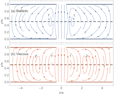
Figure 1: Vortices in a laminar (linear response) regime in ballistic (a) and viscous (b) flows in a strip geometry. Current enters the strip through a slit on one side and exits through a slit on the opposite side. Parameters used: $\gamma=0.1\,v/w$ in (a), $\gamma=100\,v/w$ in (b), the slit width equal to the strip width (see text). The two flows feature vortices of comparable intensity but different structure: two pairs of vortices in the viscous regime at $x_{1,1^{\prime}}\approx\pm w$ and $x_{2,2^{\prime}}\approx\pm 2w$ vs. one pair in the ballistic regime. The interpolated current distributions used to picture the flows, while accurately representing the flow geometry, misrepresent the vorticity magnitude. The latter is quantified by the stream functions shown in Fig.2, indicating that vorticity values are quite similar in the two regimes.

The robustness and generic character of vorticity in electron flows prompts a question of how the vortex patterns observed experimentally can be linked to the microscopic interactions and scattering mechanisms. Naively, judging from Fig.1 this may seem challenging. Indeed, despite somewhat different appearance in the viscous and ballistic phases, vortex patterns feature comparable vorticity values. However, while vorticity experiences little change upon the viscous-to-ballistic crossover, its response to momentum-relaxing collisions due to phonons or disorder is completely different in the two cases. Namely, vorticity is suppressed by momentum-relaxing scattering orders-of-magnitude more strongly in the viscous phase than in the ballistic phase. That is, a minuscule momentum-relaxing scattering is sufficient to suppress the vorticity of viscous flows, leaving vorticity of ballistic flows practically unaffected. This striking behavior can therefore serve as a diagnostic allowing to delineate between ballistic and viscous vortices.

This behavior can be readily established using the general framework of a nonlocal current-field response

$$j_{\alpha}({\boldsymbol{x}})=\int d^{2}x^{\prime}\sigma_{\alpha\beta}\left({\boldsymbol{x}}-{\boldsymbol{x}}^{\prime}\right)E_{\beta}\left({\boldsymbol{x}}^{\prime}\right).$$ (1)

As it will be clear, nonlocal conductivity is the key property responsible for the formation of vortices. Namely, vorticity of the flow reflects the $k$ dependence of conductivity no matter what origin, ballistic, viscous, or else:

$$j_{\alpha}({\boldsymbol{k}})\!\!=\!\!\sigma_{\alpha\beta}({\boldsymbol{k}})E_{\beta}({\boldsymbol{k}}),\quad\sigma_{\alpha\beta}({\boldsymbol{k}})\!\!=\!\!\int\!\!d^{2}xe^{-i{\boldsymbol{k}}{\boldsymbol{x}}}\sigma_{\alpha\beta}({\boldsymbol{x}}).$$ (2)

To the contrary, a $k$-independent conductivity describes ohmic transport with a local current-field relation; in this case the flow is potential and vortex-free. Therefore, the threshold for vorticity suppression by disorder can be inferred directly from the conductivity $k$ dependence.

To gain insight, we consider dispersive conductivity in the ballistic and viscous phases (see Eq.(7)):

$${\rm a)}\ \sigma_{\rm ball}({\boldsymbol{k}})=\frac{D}{\gamma_{0}+v|{\boldsymbol{k}}|/2};\quad{\rm b)}\ \sigma_{\rm visc}({\boldsymbol{k}})=\frac{D}{\gamma_{0}+\nu{\boldsymbol{k}}^{2}}$$ (3)

with $D=ne^{2}/m$ the Drude spectral weight and $\nu=v^{2}/4\gamma$ the kinematic viscosity. Here $\gamma_{0}$ is the momentum relaxation rate due to disorder, $\gamma$ is the electron-electron collision rate that governs viscosity, and in the viscous case the long wavelength limit $kv\ll\gamma$ is assumed. The quantity in the denominators is the disorder scattering rate $\gamma_{0}$ corrected by a $k$-dependent contribution describing momentum relaxation due to momentum spreading over the lengthscales $\ell\sim 1/k$. The $k$ values for which this contribution becomes smaller than $\gamma_{0}$ define the lengthscales beyond which the conductivity is effectively local, yielding a current flow that is potential and vortex-free.

For transport in a system of size $w$ the relevant wavenumber values, describing momentum escaping from the systems, are $k\sim 1/w$. Comparing to Eq.(3), this predicts the threshold values for disorder scattering above which the momentum dependence of conductivity is suppressed, respectively for the ballistic and viscous regimes:

$${\rm a)}\ \gamma^{\prime}_{0}\approx v/w;\quad{\rm b)}\ \gamma^{\prime\prime}_{0}\approx\nu/w^{2}.$$ (4)

Condition a) states that vorticity is supressed when the disorder mean free path is smaller than the system size. Condition b) states that the momentum relaxation time is shorter than the time momentum diffuses across viscous fluid in a system of size $w$, which is a considerably more stringent condition than a). These two threshold values are related as

$$\gamma^{\prime\prime}_{0}/\gamma^{\prime}_{0}\approx\ell_{\rm ee}/w,$$ (5)

where $\ell_{\rm ee}=v/\gamma$ is the el-el collision mean free path. We see that in a hydrodynamic regime, $\ell_{\rm ee}\ll w$, the sensitivity of vortices to momentum-relaxing collisions is orders of magnitude stronger than in the ballistic regime.

Our geometry of interest is an infinite strip of width $w,-\infty<x<\infty$, $0<y<w$, with a pair of slits on opposite sides serving as the injector and drain contacts, Fig.1. In this geometry, we will solve for the current distribution for a general nonlocal current-field linear response relation given in Eq.(1). We adopt no-slip boundary conditions modeled using a fictitious field ${\boldsymbol{E}}^{(fic)}$ concentrated at the boundary, as discussed below. The distribution of the electric field ${\boldsymbol{E}}({\boldsymbol{x}})$ that drives the current, and that of the fictitious field ${\boldsymbol{E}}^{(fic)}({\boldsymbol{x}})$ will be determined from the solution of the transport problem within the strip.

To prepare for the discussion of nonlocal transport in a strip, we first consider the properties of the $k$-dependent conductivity, Eq.(2), found by Fourier transforming the translation-invariant linear response function in Eq.(1). In general, the conductivity $\sigma_{\alpha\beta}({\boldsymbol{k}})$ takes different values for fields and currents parallel and perpendicular to the wavevector ${\boldsymbol{k}}$, such that

$$j_{\perp}(k)=\sigma_{\perp}(k)E_{\perp}(k),\quad j_{\|}(k)=\sigma_{\|}(k)\left(E_{\|}(k)-i{\boldsymbol{k}}\delta\mu(k)\right),$$

where we added a term $\delta\mu({\boldsymbol{k}})$ to describe the potential of a space charge that builds up due to the spatial nonuniformity of current. In a steady state described by a time-independent field and current, the potential $\delta\mu({\boldsymbol{x}})$, determined from the continuity relation $\text{div}{\boldsymbol{j}}=0$, cancels the longitudinal component $E_{\|}$. Namely, for a time-independent field and current there is no longitudinal current ${\boldsymbol{j}}\|{\boldsymbol{k}}$ because of charge continuity. As a result, transport is described solely by $\sigma_{\perp}({\boldsymbol{k}})$ through a relation between transverse components of ${\boldsymbol{j}}$ and ${\boldsymbol{E}}$ given by a ${\boldsymbol{k}}$-dependent conductivity:

$$\sigma_{\alpha\beta}({\boldsymbol{k}})=\sigma(k)\left(\delta_{\alpha\beta}-\hat{{\boldsymbol{k}}}_{\alpha}\hat{{\boldsymbol{k}}}_{\beta}\right).$$ (6)

From now on, for conciseness, we drop the subscript $\perp$.

The quantity $\sigma(k)$ can be found from the transport equation for quasiparticles at the Fermi surface. A direct analysis, described in Supplement, gives

$$\sigma(k)=\frac{D}{\gamma_{0}+\Gamma(k)},\quad\Gamma(k)=\frac{z}{\gamma_{1}+\frac{z}{\gamma_{2}+\frac{z}{\gamma_{3}+\ldots}}},$$ (7)

where $D=ne^{2}/m$, $z=k^{2}v^{2}/4$, and the quantities $\gamma_{m}$ are the eigenvalues of the linearized collision operator describing the relaxation rates for different harmonics of particle distribution, $\delta f_{\theta}({\boldsymbol{x}},t)=e^{i{\boldsymbol{k}}{\boldsymbol{x}}-i\omega t}\sum_{m}e^{-\gamma_{m}t}\delta f_{m}e^{im\theta}$, where $\theta$ is the azimuthal angle on the Fermi surface.

This general form of $\sigma(k)$ describes a variety of different regimes of interest. The rate $\gamma_{0}$ describes momentum relaxation due to disorder of phonon scattering, the quantity $\Gamma(k)$ describes relaxation of momentum by particles transporting it away from the region of interest. Here, for simplicity, we consider the case of equal rates, $\gamma_{1}=\gamma_{2}=...\equiv\gamma$, adequate for exploring vorticity in the viscous, ballistic and ohmic phases, as well as in the crossover between these phases. In this case, the quantity $\Gamma(k)$ is readily evaluated, giving

$$\Gamma(k)=\frac{-\gamma+\sqrt{\gamma^{2}+k^{2}v^{2}}}{2}.$$ (8)

The $k$-dependent conductivity $\sigma(k)$ defines a scale-dependent linear response. At small $k$ (large lengthscales) such that $\Gamma(k)<\gamma_{0}$ it describes ohmic dissipation due to disorder scattering. At large $k$ (small lengthscales) such that $\Gamma(k)>\gamma_{0}$ it describes momentum dissipation due to particle transport within the system. The large-$k$ behavior can be either ballistic or fluid-like, depending on the ratio of $\gamma$ and $kv$. Namely, for $\gamma\ll vk$ we have $\Gamma(k)=|k|v/2$, giving an expression in Eq.(3) a), whereas for $\gamma\gg vk$ we have $\Gamma(k)=k^{2}v^{2}/4\gamma$, giving an expression in Eq.(3) b).

For transport in a strip of width $w$ the characteristic wavenumber is $k\approx 1/w$. Accordingly, in our simulation we will use $\gamma=0.1v/w$ and $100v/w$ to model the ballistic and hydrodynamic regimes, respectively; the values $\gamma=1v/w$ and $10v/w$ will be used to model the crossover between these regimes.

Next we discuss the strategy for tackling the nonlocal transport problem in a strip. This problem will be dealt with by replacing the strip geometry with an infinite 2D plane geometry and, simultaneously, introducing suitable boundary conditions to make the infinite-space problem mimic that for the finite-width strip. Passing to the infinite-space setting allows to fully benefit from the translation invariance of the current-field relation, Eq.(1). The latter then becomes an exact property and can be conveniently handled in a Fourier representation.

To tackle the boundary-value problem in the infinite-space representation, we employ Eq.(1), with an electric field corrected by a fictitious electric field of value chosen to null the current at the boundary:

$$E_{\beta}({\boldsymbol{x}})\!=\!E_{\beta}^{(ext)}({\boldsymbol{x}})\!-\!E_{\beta}^{(fic)}({\boldsymbol{x}}),\ \ E_{\beta}^{(fic)}\left({\boldsymbol{x}}\right)\!=\!\lambda j_{\beta}({\boldsymbol{x}}),$$ (9)

where the fictitious field $E_{\beta}^{(fic)}({\boldsymbol{x}})$ is defined at system boundary through a relation with the current at the boundary, with $\lambda$ a ‘boundary resistivity’ parameter (see [20, 21]). We will derive and solve equations that are valid for any $\lambda$. Then, in the numerical analysis of the results we will take a large enough value for this parameter ($\lambda=10^{5}v$) to simulate non-slip boundary conditions. The field $E_{\beta}^{(ext)}$ is a constant external field along the $y$ axis, it can be integrated over, leaving an additive term $j_{\alpha}^{(ext)}=j_{0}\delta_{\alpha,y}$, which is the current that we inject into our system.

It is convenient, for the purpose of analysis, to rewrite the current-field relations with the fictitious boundary fields, Eq.(9), by introducing a window function for the slit $\chi(x)=1$ for $|x|\geq w/2$, and $0$ for $|x|<w/2$. Since the fictitious field exists only at the strip boundaries $y=0$ and $w$, Eqs.(1) and (9), relate currents in the strip bulk and currents at the boundaries:

$$j_{\alpha}({\boldsymbol{x}}) =j_{0}\delta_{\alpha,y}-\lambda\int d{\boldsymbol{x}^{\prime}}\delta(y^{\prime})\chi\left(x^{\prime}\right)\sigma_{\alpha\beta}\left({\boldsymbol{x}}-{\boldsymbol{x}^{\prime}}\right)j_{\beta}({\boldsymbol{x}^{\prime}})$$

$$-\lambda\int d{\boldsymbol{x}^{\prime}}\delta(y^{\prime}-w)\chi\left(x^{\prime}\right)\sigma_{\alpha\beta}\left({\boldsymbol{x}}-{\boldsymbol{x}^{\prime}}\right)j_{\beta}({\boldsymbol{x}^{\prime}})$$ (10)

The symmetry of the strip with a pair of slits imposes the relations for the components of the current,

$$j_{y}(y,x)=j_{y}(y,-x);\hskip 14.22636ptj_{y}(y,x)=j_{y}(w-y,x)$$ (11)

$$j_{x}(y,x)=-j_{x}(y,-x);\hskip 14.22636ptj_{x}(y,x)=-j_{x}(w-y,x)$$ (12)

Eqs.(Robustness of vorticity in electron fluids) for these quantities can be Fourier-transformed to obtain integral equations for the Fourier harmonics of currents at the boundaries $j_{\alpha}(x,y)=\int\frac{dq}{2\pi}j_{\alpha}(q,y)e^{-iqx}$:

$$j_{y}(q,y)= 2\pi j_{0}\delta(q)-\lambda\Sigma_{yy}(q)\left(\tilde{\chi}\left(q\right)*j_{y}(q,0)\right)$$

$$+i\lambda\Sigma_{yx}(q)\left(\tilde{\chi}\left(q\right)*j_{x}(q,0)\right)$$ (13)

$$j_{x}(q,y)= -\lambda\Sigma_{xx}(q)\left(\tilde{\chi}\left(q\right)*j_{x}(q,0)\right)$$

$$+i\lambda\Sigma_{xy}(q)\left(\tilde{\chi}\left(q\right)*j_{y}(q,0)\right)$$ (14)

(for the derivation, see Supplement). Here we used the symmetry relations for current components at $y=0$ and $w$ to eliminate the $y=w$ quantities in favor of the $y=0$ quantities. We also introduced Fourier harmonics of the slit window function $\tilde{\chi}\left(q\right)=\int dx\chi\left(x\right)e^{iqx}=2\pi\left(\delta(q)-\frac{1}{\pi}\frac{\sin(qw)}{q}\right)$. The notation $*$ stands for the convolution $(\tilde{\chi}\left(q\right)*j_{\alpha}(q,0))=\int_{-\infty}^{\infty}\tilde{\chi}\left(q-q^{\prime}\right)j_{\alpha}(q^{\prime},0)dq^{\prime}$, and the quantities $\Sigma_{ii^{\prime}}(q)$ are defined as

$$\Sigma_{yy}(q)=\int\frac{dk_{y}}{2\pi}\left[\cos\left(k_{y}y\right)+\cos\left(k_{y}\left(w-y\right)\right)\right]\frac{\sigma\left(\kappa\right)q^{2}}{\kappa^{2}};\hskip 7.11317pt\Sigma_{yx}(q)=\int\frac{dk_{y}}{2\pi}\left[\sin\left(k_{y}y\right)+\sin\left(k_{y}\left(w-y\right)\right)\right]\frac{\sigma\left(\kappa\right)qk_{y}}{\kappa^{2}}$$ (15)

$$\Sigma_{xx}(q)=\int\frac{dk_{y}}{2\pi}\left[\cos\left(k_{y}y\right)-\cos\left(k_{y}\left(w-y\right)\right)\right]\frac{\sigma\left(\kappa\right)k_{y}^{2}}{\kappa^{2}};\hskip 7.11317pt\Sigma_{xy}(q)=\int\frac{dk_{y}}{2\pi}\left[\sin\left(k_{y}y\right)-\sin\left(k_{y}\left(w-y\right)\right)\right]\frac{\sigma\left(\kappa\right)qk_{y}}{\kappa^{2}}$$ (16)

where we introduced notation $\kappa^{2}=q^{2}+k_{y}^{2}$.

The right-hand side in Eqs.(13) and (14) contains only the currents on the lower boundary $y=0$. We therefore set $y=0$ to obtain a pair of coupled linear integral equations for $j_{x}(q,0)$ and $j_{y}(q,0)$. Because of the convolution these integral equations cannot be solved analytically, therefore a numerical approach must be used. For this we introduce an interval $-L/2<x<L/2$ on the $x$-axis, discretized with a mesh of spacing $L/N$ with a large enough $N$. For the functions in this interval we assume periodic boundary conditions. In Fourier representation, these functions are sums of harmonics with a discrete set of wavenumbers chosen as $q_{i}=\left(i-\frac{N-1}{2}\right)\Delta q\prime$, $i=1,2,...,N$ with a step size $\Delta q^{\prime}=2\pi/L$. We solve our equations on this dual lattice, approximating integrals as Riemann sums. An inverse Fourier transform is then carried out to find the currents in interval $-L/2<x<L/2$ in real space. Thanks to the discretization the convolution in each Eqs.(13),(14) yields a linear operator representing the corresponding integral by a $N\times N$ matrix. This allows us to solve the resulting linear equations by inverting matrices.

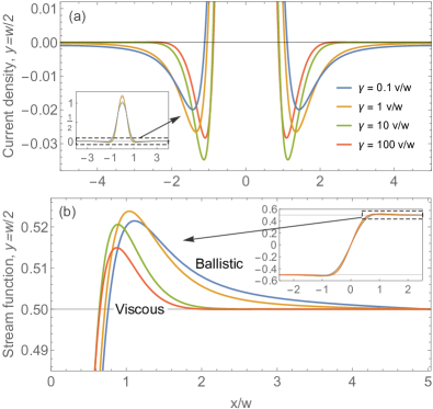
Figure 2: (a) Current backflow in the viscous, ballistic and intermediate regimes on the line $y=w/2$ in the middle of the strip. The backflow magnitude is nearly the same in all regimes, being slightly larger in the intermediate regime than in the viscous and ballistic regimes. (b) Stream function $\phi_{y=w/2}(x)$ normalized as $\phi_{y=w/2}(x)|^{L/2}_{-L/2}=1$ for different regimes, detailing the backflows. The largest magnitude is for $\gamma=1v/w$ (intermediate regime). The inset shows the full stream function.

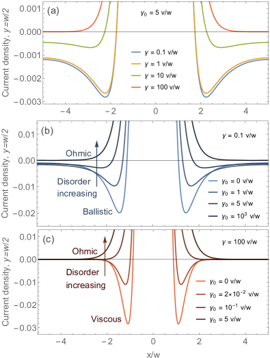
Figure 3: Suppression of current backflow and vorticity by ohmic dissipation in different regimes. (a) Current in the middle of the strip at a fixed disorder scattering rate $\gamma_{0}=5\,v/w$ and varying $\gamma$. The backflow and vorticity survive in the ballistic regime but are completely suppressed in the viscous regime. (b),(c) Weakening of the backflow upon increasing ohmic scattering in the ballistic and viscous regimes (realized at $\gamma=0.1\,v/w$ and $\gamma=100\,v/w$, respectively). Ballistic backflow is weakened roughly 2 times for $\gamma_{0}=1\,v/w$, and totally suppressed for $\gamma_{0}=10^{3}\,v/w$. Viscous backflow is considerably more fragile, being weakened roughly 2 times for $\gamma_{0}=2\times 10^{-2}\,v/w$ and completely suppressed for $\gamma_{0}=5\,v/w$.

We first consider the results for the disorder-free case ($\gamma_{0}=0$ in (7)). After solving for currents at $y=0$ as described in Supplement we use (13), (14) to find currents in the strip bulk. Below we discuss the behavior on a line in the middle of the strip $y=w/2$. The resulting current profile, pictured in Fig.2(a) shows that on both sides of the direct current flowing from injector to drain there are regions where current flows against the applied field, signaling the presence of vortices. Vortices are seen to be present in both the ballistic and viscous regime. Notably, the vortices have similar intensities in the two regimes, with a little change at the crossover.

One difference between vortices in the two regimes is in their spatial extent: ballistic vortices are about $\sim 2$ times wider than viscous vortices. Another (minor) difference is that current undergoes multiple sign reversals, indicating the presence of several vortices of opposite orientation (so-called Moffatt vortices[23, 24]). This confirms the presence of multiple vortices in the viscous regime, in line with the flow pictured in Fig.1. However, Fig.2 also indicates that the secondary vortices are extremely weak, illustrating that Fig.1 predicts correctly the flow geometry but misrepresents the magnitude of vorticity.

To gain more insight, we consider the stream function defined through ${\boldsymbol{u}}=\nabla\times(\phi({\boldsymbol{x}})\hat{z})=(\partial_{y}\phi({\boldsymbol{x}}),-\partial_{x}\phi({\boldsymbol{x}}))^{\rm T}$, where ${\boldsymbol{j}}=en{\boldsymbol{u}}$ [see Fig. 2(b)]. This quantity has a number of useful properties. In particular, it quantifies the net integrated backflow regardless of how far from the slit the backflow occurs and the details of its spatial distribution and, as such, provides a meaningful comparison between different regimes. This quantity, shown in Fig. 2(b) on the line in the middle of the strip, $\phi_{w/2}(x)=\int_{0}^{x}j_{y}(\xi,w/2)d\xi$ indicates a larger swing for the ballistic flow (blue curve) than the viscous flow (red curve), i.e. the backflow is actually somewhat stronger in the ballistic case than in the viscous case. Yet, in the absence of disorder scattering, the predicted differences between ballistic and viscous vortices are probably not strong enough to unambiguously differentiate these regimes experimentally.

Yet, the ballistic and viscous vortices behave very differently in the presence of disorder scattering (ohmic dissipation). Namely, a relatively weak disorder scattering is sufficient to suppress viscous vortices, while having little impact on ballistic vortices, as illustrated in Fig. 3. Usually, disorder scattering is nearly temperature-independent, whereas the el-el scattering is strongly temperature dependent (behaving as $\sim T^{2}$ in Landau Fermi-liquids). This means that the quantity $\gamma$ can be tuned by varying temperature, while keeping $\gamma_{0}$ approximately constant. As an illustration we set $\gamma_{0}=5\,v/w$ and vary $\gamma$ (see Fig. 3(a)). We see that this dissipation value is enough to fully suppress viscous backflow (red line), while reducing the ballistic backflow (blue line) only by $\sim 5$ times. The property of ballistic vortices to be more resilient than viscous vortices in the presence of ohmic dissipation suggests a simple and direct diagnostic allowing to discriminate the two regimes in experiment.

It is also instructive to consider how ballistic and viscous vortices, which have approximately equal intensity in the absence of ohmic dissipation, are suppressed as the disorder scattering rate $\gamma_{0}$ increases, see Fig. 3 (b) and (c). In both cases we observe a transition to the ohmic flow regime that shows no backflow. Yet, the values $\gamma_{0}$ above which the flow becomes effectively Ohmic are very different for the two cases. Ballistic vortices are quite robust and can endure disorder scattering as high as $\gamma_{0}=10^{3}\,v/w$. Viscous vortices, to the contrary, are affected significantly by much smaller ohmic dissipation. E.g., dissipation as small as $\gamma_{0}=2\times 10^{-2}\,v/w$ results in a loss of the second (Moffatt) vortex and weakens the backflow amplitude 2 times, while for the ballistic case a similar reduction of the backflow happens only for $\gamma_{0}=1\,v/w$. These values are in a good agreement with the simple estimates given above in Eq.(3).

In summary, vorticity of a current flowing in a restricted geometry is a salient feature arising due to the nonlocal $k$-dependent conductivity that governs the current-field relation. As such, it is present and takes similar values in the ballistic and viscous transport regimes. We expect the qualitative behavior found in the strip geometry — similar intensity for vorticity in the ballistic regime and in the viscous regime, the resilience of ballistic vortices in the presence of ohmic dissipation and the comparatively more fragile behavior of viscous vortices — to hold in any realistic geometry. The strikingly different dependence of vortex flows on el-el scattering and ohmic dissipation is an observable signature that can be used to discriminate the origin of vorticity in electron fluids.

We thank M. Davydova, G. Falkovich and E. Zeldov for inspiring discussions. This work was supported by the Science and Technology Center for Integrated Quantum Materials, NSF Grant No. DMR1231319; Army Research Office Grant W911NF-18-1-0116; and Bose Foundation Research fellowship.

Supporting Material for ”Robustness of vorticity in electron fluids”

I Scale dependent conductivity and continued fractions

Here we derive a relation between nonlocal conductivity $\sigma(k)$ and the relaxation times for different angular harmonics of carrier distribution, which is used in the main text. As a starting point, we use the quantum Boltzmann equation for electrons in the presence of an external electric field, linearized in small deviations of carrier distribution from equilibrium:

$$\left(\partial_{t}+{\boldsymbol{v}}\nabla_{{\boldsymbol{x}}}-I\right)\delta f_{{\boldsymbol{p}}}(t,{\boldsymbol{x}})=-e{\boldsymbol{E}}\nabla_{{\boldsymbol{p}}}f_{{\boldsymbol{p}}}^{(0)}$$ (17)

where $f_{{\boldsymbol{p}}}^{(0)}$ is the equilibrium distribution, and $I$ is the collision operator. In what follows it will be convenient to rewrite the expression on the right-hand side as ${\boldsymbol{E}}\nabla_{{\boldsymbol{p}}}f_{{\boldsymbol{p}}}^{(0)}={\boldsymbol{E}}{\boldsymbol{v}}\left(\partial f_{{\boldsymbol{p}}}^{(0)}/\partial\epsilon\right)$. The perturbed distribution can be decomposed into a sum of cylindrical harmonics as $\delta f_{{\boldsymbol{p}}}=e^{i{\boldsymbol{k}}{\boldsymbol{x}}-i\omega t}\sum_{m}\delta f_{m}e^{im\theta}$, where $\theta$ is the azimuthal angle on the Fermi surface. Due to the cylindrical symmetry, the harmonics $\delta f_{m}e^{im\theta}$ are eigenfunctions of the collision operator,

$$I\delta f_{m}e^{im\theta}=-\gamma_{m}\delta f_{m}e^{im\theta},$$ (18)

where $\gamma_{m}$ are relaxation rates originating from microscopic processes of carrier scattering and collisions. For instance, $\gamma_{1}$ originates from momentum relaxation due to disorder of phonon scattering, $\gamma_{2}$ is due to electron-electron collisions, $\gamma_{0}=0$ due to particle number conservation, and so on.

It will be convenient to use the basis $\delta f_{m}e^{im\theta}$ to bring the problem to the form described by a tridiagonal matrix, a representation in which a closed-form solution for conductivity $\sigma(k)$ can be given in terms of continued fractions. This representation is obtained by noting that the terms ${\boldsymbol{v}}{\boldsymbol{k}}$ and $e{\boldsymbol{v}}{\boldsymbol{E}}$, when rewritten in the angular harmonics basis, have nonzero matrix elements only between harmonics $m$ and $m\pm 1$. This is made apparent by the identities

$${\boldsymbol{v}}{\boldsymbol{k}} =\frac{v}{2}\left(k_{x}+ik_{y}\right)e^{-i\theta}+\frac{v}{2}\left(k_{x}-ik_{y}\right)e^{i\theta}=\zeta e^{-i\theta}+\bar{\zeta}e^{i\theta}$$ (19)

$$e{\boldsymbol{v}}{\boldsymbol{E}} =\frac{ev}{2}\left(E_{x}+iE_{y}\right)e^{-i\theta}+\frac{ev}{2}\left(E_{x}-iE_{y}\right)e^{i\theta}=\mathcal{E}e^{-i\theta}+\bar{\mathcal{E}}e^{i\theta}$$ (20)

where we introduced $\zeta=v(k_{x}+ik_{y})/2$, $\mathcal{E}=ev\left(E_{x}+iE_{y}\right)/2$. Accordingly, the Boltzmann equation turns into a system of coupled linear equations:

$$\gamma_{m}\delta f_{m}+\zeta\delta f_{m+1}+\bar{\zeta}\delta f_{m-1}=\frac{\partial f_{\textbf{p}}^{(0)}}{\partial\epsilon}\left(\mathcal{E}\delta_{m,-1}+\bar{\mathcal{E}}\delta_{m,1}\right)$$ (21)

This problem describes a response of variables $\delta f_{m}$ to the “source” $\mathcal{E}\delta_{m,-1}+\bar{\mathcal{E}}\delta_{m,1}$. To solve these equations, we first consider the source term with $m=1$, adding the contribution of the source term with $m=-1$ later. We introduce $\alpha_{m}=i\delta f_{m+1}/\delta f_{m}$, which brings equations with $m>1$ to the form

$$\gamma_{m}+\zeta\alpha_{m}-\frac{\bar{\zeta}}{\alpha_{m-1}}=0$$ (22)

These equations give a simple recursion equation $\alpha_{m-1}=\frac{\bar{\zeta}}{\gamma_{m}+\zeta\alpha_{m}}$, which can be solved iteratively over $m+1,m+2,\dots$ giving a continued fraction

$$\alpha_{m-1}=\frac{\bar{\zeta}}{\gamma_{m}+\frac{\left|\zeta\right|^{2}}{\gamma_{m+1}+\frac{\left|\zeta\right|^{2}}{\gamma_{m+2}+\dots}}}$$ (23)

Similarly, for $m<1$ we define $\beta_{m}=i\delta f_{m-1}/\delta f_{m}$ and obtain

$$\beta_{m+1}=\frac{\zeta}{\gamma_{m}+\frac{\left|\zeta\right|^{2}}{\gamma_{m-1}+\frac{\left|\zeta\right|^{2}}{\gamma_{m-2}+\ldots}}}$$ (24)

Now, the harmonic $\delta f_{1}$ can be found from the $m=1$ equation

$$\gamma_{1}\delta f_{1}+i\zeta\delta f_{2}+i\bar{\zeta}\delta f_{0}=\frac{\partial f_{\textbf{p}}^{(0)}}{\partial\epsilon}{\mathcal{E}}.$$ (25)

Rewriting it as $\delta f_{1}\left(\gamma_{1}+\zeta\alpha_{1}+\bar{\zeta}\beta_{1}\right)=\frac{\partial f_{\textbf{p}}^{(0)}}{\partial\epsilon}\mathcal{E}$ and substituting the continued fractions for $\alpha_{1}$ and $\beta_{1}$ yields

$$\delta f_{1}=\frac{\partial f_{\textbf{p}}^{(0)}}{\partial\epsilon}\frac{\mathcal{E}}{\gamma_{1}+\frac{|\zeta|^{2}}{\gamma_{2}+\frac{|\zeta|^{2}}{\gamma_{3}+\frac{|\zeta|^{2}}{\gamma_{4}++\ldots}}}+\frac{|\zeta|^{2}}{\gamma_{0}+\frac{|\zeta|^{2}}{\gamma_{-1}+\frac{|\zeta|^{2}}{\gamma_{-2}+\ldots}}}}=\frac{\partial f_{\textbf{p}}^{(0)}}{\partial\epsilon}\frac{\mathcal{E}}{2\gamma_{1}+\frac{2|\zeta|^{2}}{\gamma_{2}+\frac{|\zeta|^{2}}{\gamma_{3}+\frac{|\zeta|^{2}}{\gamma_{4}++\ldots}}}},$$ (26)

where we used the identities $\gamma_{-m}=\gamma_{m}$ and $\gamma_{0}=0$ that account for the inversion symmetry and particle number conservation. The contribution of the $m=-1$ source term, found in a similar manner, is given by an expression identical to Eq.(26) up to a replacement of $\mathcal{E}$ with $\bar{\mathcal{E}}$.

With this it is straightforward to obtain the nonlocal conductivity by combining the current density $j_{y,k}=ev\nu_{0}\oint(d\theta/2\pi)\sin\theta\delta f(\theta)$ and the definition of conductivity ${\boldsymbol{j}}_{{\boldsymbol{k}}}=\sigma(k,\omega){\boldsymbol{E}}_{{\boldsymbol{k}}}$. We find

$$\sigma(k)=\frac{D}{\gamma_{0}+\Gamma(k)},\quad\Gamma(k)=\frac{z}{\gamma_{1}+\frac{z}{\gamma_{2}+\frac{z}{\gamma_{3}+\ldots}}}$$ (27)

with $D=ne^{2}/m$ the Drude weight and $z=k^{2}v^{2}/4$.

The quantity $\Gamma(k)$ can be evaluated in a closed form for the model $\gamma_{2}=\gamma_{3}=...\equiv\gamma$. In this case, a simple recursion relation yields $\Gamma(k)=z/(\gamma+\Gamma(k))$, solved by

$$\Gamma(k)=\frac{-\gamma+\sqrt{\gamma^{2}+k^{2}v^{2}}}{2}.$$ (28)

This gives a scale-dependent conductivity used in the main text:

$$\sigma(k)=\frac{2D}{2\gamma_{0}+\sqrt{v^{2}k^{2}+\gamma^{2}}-\gamma},$$ (29)

where we replaced $\gamma_{1}$ with $\gamma_{0}$ to make the notation agree with that in the main text.

II Equations for current components in the strip geometry

Here we detail the procedure used to evaluate the nonlocal response in the strip geometry. We will work in the mixed representation defined in the main text – Fourier components along the strip ($x$) and direct-space normal to the strip ($y$). This representation is found by passing from the system with a boundary to an infinite plane, replacing boundary conditions with an fictitious electric field as described in the man text. This gives coupled equations for different current components:

$$j_{\alpha}({\boldsymbol{x}})= j_{0}\delta_{\alpha,y}-\lambda\int d{\boldsymbol{x}^{\prime}}\delta(y^{\prime})\chi\left(x^{\prime}\right)\sigma_{\alpha\beta}\left({\boldsymbol{x}}-{\boldsymbol{x}^{\prime}}\right)j_{\beta}({\boldsymbol{x}^{\prime}})-\lambda\int d{\boldsymbol{x}^{\prime}}\delta(y^{\prime}-w)\chi\left(x^{\prime}\right)\sigma_{\alpha\beta}\left({\boldsymbol{x}}-{\boldsymbol{x}^{\prime}}\right)j_{\beta}({\boldsymbol{x}^{\prime}}),$$

where $\chi\left(x^{\prime}\right)=1$ if $x^{\prime}\geq w/2$, and zero for $x^{\prime}<w/2$.

We first consider the $y$ component:

$$j_{y}({\boldsymbol{x}}) =j_{0}-\lambda\int d{\boldsymbol{x}^{\prime}}\delta(y^{\prime})\chi\left(x^{\prime}\right)\sigma_{yy}\left({\boldsymbol{x}}-{\boldsymbol{x}^{\prime}}\right)j_{y}({\boldsymbol{x}^{\prime}})-\lambda\int d{\boldsymbol{x}^{\prime}}\delta(y^{\prime}-w)\chi\left(x^{\prime}\right)\sigma_{yy}\left({\boldsymbol{x}}-{\boldsymbol{x}^{\prime}}\right)j_{y}({\boldsymbol{x}^{\prime}})$$

$$-\lambda\int d{\boldsymbol{x}^{\prime}}\delta(y^{\prime})\chi\left(x^{\prime}\right)\sigma_{yx}\left({\boldsymbol{x}}-{\boldsymbol{x}^{\prime}}\right)j_{x}({\boldsymbol{x}^{\prime}})-\lambda\int d{\boldsymbol{x}^{\prime}}\delta(y^{\prime}-w)\chi\left(x^{\prime}\right)\sigma_{yx}\left({\boldsymbol{x}}-{\boldsymbol{x}^{\prime}}\right)j_{x}({\boldsymbol{x}^{\prime}}).$$ (30)

Substituting conductivity by the Fourier representation,

$$\sigma_{\alpha\beta}\left({\boldsymbol{x}}-{\boldsymbol{x}^{\prime}}\right)=\int\frac{dk_{x}dk_{y}}{(2\pi)^{2}}e^{ik_{x}\left(x-x^{\prime}\right)}e^{ik_{y}\left(y-y^{\prime}\right)}\sigma_{\alpha\beta}({\boldsymbol{k}}),$$ (31)

and integrating over $y^{\prime}$, gives

$$j_{y}(x,y) =j_{0}-\lambda\int\frac{dk_{x}dk_{y}}{(2\pi)^{2}}\int dx^{\prime}\chi\left(x^{\prime}\right)j_{y}(x^{\prime},0)e^{ik_{x}\left(x-x^{\prime}\right)}e^{ik_{y}y}\left(1+e^{-ik_{y}w}\right)\sigma_{yy}({\boldsymbol{k}})$$

$$-\lambda\int\frac{dk_{x}dk_{y}}{(2\pi)^{2}}\int dx^{\prime}\chi\left(x^{\prime}\right)j_{x}(x^{\prime},0)e^{ik_{x}\left(x-x^{\prime}\right)}e^{ik_{y}y}\left(1-e^{-ik_{y}w}\right)\sigma_{yx}({\boldsymbol{k}}).$$ (32)

Here we have used spatial mirror symmetries of the current density components: $j_{x}(x,w)=-j_{x}(x,0)$ and $j_{y}(x,w)=j_{y}(x,0)$.

Next we carry out a Fourier transform over $x$, $j_{y}(q,y)=\int j_{y}(x,y)e^{-iqx}dx$, to obtain

$$j_{y}(q,y) =2\pi j_{0}\delta(q)-\lambda\left(\int dx^{\prime}\chi\left(x^{\prime}\right)j_{y}(x^{\prime},0)e^{-iqx^{\prime}}\right)\left(\int\frac{dk_{y}}{2\pi}\left(e^{ik_{y}y}+e^{ik_{y}\left(y-w\right)}\right)\sigma_{yy}(q,k_{y})\right)$$

$$-\lambda\left(\int dx^{\prime}\chi\left(x^{\prime}\right)j_{x}(x^{\prime},0)e^{-iqx^{\prime}}\right)\left(\int\frac{dk_{y}}{2\pi}\left(e^{ik_{y}y}-e^{ik_{y}\left(y-w\right)}\right)\sigma_{yx}(q,k_{y})\right).$$ (33)

At the last step we use the relations $\sigma_{\alpha\beta}(q,-k_{y})=-\sigma_{\alpha\beta}(q,k_{y})$ for $\alpha\neq\beta$ and $\sigma_{\alpha\beta}(q,-k_{y})=\sigma_{\alpha\beta}(q,k_{y})$ for $\alpha=\beta$. Hence, in the second term we may replace $\left(e^{ik_{y}y}+e^{ik_{y}\left(y-w\right)}\right)$ with $\left(\cos\left(k_{y}y\right)+\cos\left(k_{y}\left(w-y\right)\right)\right)$, and similarly in the third term $\left(e^{ik_{y}y}-e^{ik_{y}\left(y-w\right)}\right)$ with $i\left(\sin\left(k_{y}y\right)+\sin\left(k_{y}\left(w-y\right)\right)\right)$, since the remaining parts will be nulled due to parity of the integrals. Moreover, we can notice that $\int dx^{\prime}\chi\left(x^{\prime}\right)j_{y}(x^{\prime},0)e^{-iqx^{\prime}}=\tilde{\chi}\left(q\right)*j_{y}(q,0)$ is convolution in the $q$-space. Using the similar approach for the $j_{x}(q,y)$ we will obtain the relations given in Eqs.(13), (14) of the main text. These relations express the currents in the interior of the strip $0<y<w$ through the currents at the lower boundary $y=0$. To determine the currents in the strip interior we first determine currents at the boundary, and then use the above bulk/boundary relations to find currents in the entire strip. This procedure is detailed and illustrated in Sec.III.

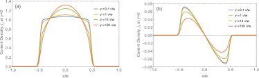
Figure 4: Current distributions at the boundary $y=0$ in the dissipation-less dynamics $\gamma_{0}=0$ for the viscous, ballistic and intermediate regimes. (a), (b) show the current components along the $y$ and $x$ axes, respectively

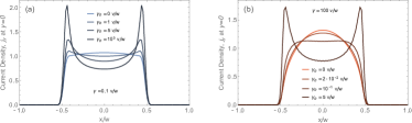
Figure 5: Current distributions along the $y$ axis at the boundary $y=0$ for increasing disorder scattering (a) ballistic to ohmic crossover (b) viscous to ohmic crossover

III Finding currents at the strip boundary

Here we introduce the approach used for solving the equations (13), (14). The right-hand side in both of these equations contains only the currents at the lower boundary $y=0$. Therefore, we set $y=0$ to obtain a pair of coupled linear integral equations for $j_{x}(q,0)$ and $j_{y}(q,0)$. After the discretization in the $q$ space introduced in the main text the currents $j_{x}(q,0)$, $j_{y}(q,0)$ become vectors with $N$ elements and the convolution becomes a linear operator representing the corresponding integral by a $N\times N$ matrix: $\tilde{\chi}\left(q\right)*j_{y}(q,0)\to\hat{M}_{\chi}j_{y}(q,0)$. This rewrites the current equations in a form:

$$j_{y}(q,0) =2\pi j_{0}\delta(q)-\lambda\hat{M}_{\chi}\Sigma_{yy}(q)j_{y}(q,0)+i\lambda\hat{M}_{\chi}\Sigma_{yx}(q)j_{x}(q,0)$$ (34)

$$j_{x}(q,0) =-\lambda\hat{M}_{\chi}\Sigma_{xx}(q)j_{x}(q,0)+i\lambda\hat{M}_{\chi}\Sigma_{xy}(q)j_{y}(q,0)$$ (35)

To solve these equations we need to address several technical issues. First of all, in the absence of ohmic dissipation ($\gamma_{0}=0$) the quantity $\Sigma_{yy}(q)$ diverges when $q\to 0$. This problem can be eliminated either by introducing an infinitesimal $\gamma_{0}$ or by multiplying (34) by $\Sigma_{yy}^{-1}(q)$, which provides a regularization since $\Sigma_{yy}^{-1}(0)=0$. In order treat all the regimes on an equal footing we adopt the second approach. However, since $\Sigma_{yy}^{-1}(0)=0$, the term $j_{0}\Sigma_{yy}^{-1}(q)\delta(q)$ appears to vanish at all $q$, both zero and non-zero, due to the property of the $\delta$-function. Naively, this poses a problem, because the equations seem to loose the information about the injected current. However, we recall that ${\boldsymbol{j}_{0}}$ originated from an external electric field ${\boldsymbol{E}}^{(ext)}$ through $\int d^{2}{\boldsymbol{x}^{\prime}}\sigma_{\alpha\beta}\left({\boldsymbol{x}}-{\boldsymbol{x}}^{\prime}\right)E_{\beta}^{(ext)}\left({\boldsymbol{x}}^{\prime}\right)$. This integral diverges as well, and in fact, it is equal to $\Sigma_{yy}(0)$. As a result the product $j_{0}\Sigma_{yy}^{-1}(q)$ has a finite limit at $q\to 0$, and hence, $j_{0}\Sigma_{yy}^{-1}(q)\delta(q)$ can be legitimately replaced by $E^{(ext)}\delta(q)$.

The second issue that needs to be addressed is with $\Sigma_{xx}(q)$. This quantity, for $y=0$, diverges logarithmically for arbitrary $q$. The divergence originates from $k_{y}\to\infty$, i.e. the small length scales. This problem is treated by introducing a finite thickness $a$ for the boundaries. From physical perspective we conclude that for a small enough $a$, $j_{x}(q,a)\approx j_{x}(q,0)$, which allows to evaluate $\Sigma_{xx}(q)$ by plugging into the equation (16) $y=a$ instead of $y=0$:

$$\Sigma_{xx}(q)=\int\frac{dk_{y}}{2\pi}\big{[}\cos\left(k_{y}y\right)-\cos\left(k_{y}\left(w-y\right)\right)\big{]}\big{|}_{y=a}\frac{\sigma\left(\sqrt{q^{2}+k_{y}^{2}}\right)k_{y}^{2}}{q^{2}+k_{y}^{2}}$$ (36)

This integral converges for large $k_{y}$ and shows a logarithmic dependence on the scale $a$. In our numerical calculation we take $a=\Delta x/10$, where $\Delta x$ is the lattice step size in direct space.

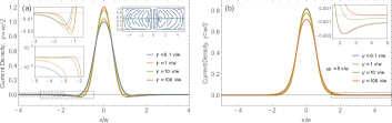
Figure 6: Current distributions at $y=w/2$. (a) Dynamics without ohmic dissipation $\gamma_{0}=0$. The left insets zoom on the backflows. The right inset shows vortices in our geometry with the horizontal line indicating the line at which the current distributions are calculated. (b) Dynamics with ohmic dissipation rate $\gamma_{0}=5v/w$. The left insets zoom on the backflows. The vorticity in the viscous regime is completely suppressed, while in the ballistic regime it is reduced $\sim 5$ times.

After these adjustments we can solve the equations (34),(35). From the eq. (35) we find

$$j_{x}(q,0)=i\lambda\left(1+\lambda\hat{M}_{\chi}\Sigma_{xx}(q)\right)^{-1}\hat{M}_{\chi}\Sigma_{xy}(q)j_{y}(q,0)$$ (37)

Then we plug it into (34) (multiplied by $\Sigma^{-1}_{yy}(q)$):

$$j_{y}(q,0)= 2\pi E^{(ext)}\left(\Sigma^{-1}_{yy}(q)+\lambda\hat{M}_{\chi}+\lambda^{2}\Sigma^{-1}_{yy}(q)\hat{M}_{\chi}\Sigma_{yx}(q)\left(1+\lambda\hat{M}_{\chi}\Sigma_{xx}(q)\right)^{-1}\hat{M}_{\chi}\Sigma_{xy}(q)\right)^{-1}\delta(q)$$ (38)

which we then use in (37) to find the $x$ component. For the final step we carry out an inverse Fourier transform of the currents. In the presence of ohmic losses, the problem with divergent $\Sigma_{yy}(q)$ does not occur, and the equations can be treated similarly but without multiplying by $\Sigma_{yy}^{-1}(q)$.

The results of this calculation are presented in Fig.4 and Fig.5. Current at the boundary vanishes outside the slit, as expected, and has an interesting profile within the slit that reflects the interplay between different scattering mechanisms. The dependence $j_{y}(x)$ is nearly flat in the ballistic regime, as expected from Sharvin’s phase space argument, and acquires a convex profile as the el-el collision rate grows, see Fig.4(a). In this limit, current drops as $x$ approches the slit edges, as expected for a viscous flow with no-slip boundary conditions. The sign-changing profile of $j_{x}(x)$ indicates that within the slit on the $y=0$ boundary the current flows towards $x=0$ vertical axis, see Fig.4(b). As can be seen in Fig.1 of the main text, the convergence towards the central vertical axis is replaced by a divergence form it at a slightly larger $y$. This behavior persists in the strip interior up to the middle line $y=w/2$; above this line the current flow is a mirror image of that below the line $y=w/2$, such that $j_{x}(x,y)=-j_{x}(x,w-y)$ and $j_{y}(x,y)=j_{y}(x,w-y)$. The profile $j_{y}(x)$ in the slit undergoes an interesting transformation when ohmic losses are introduced, developing a double-horn structure in both the ballistic and viscous regimes as the disorder scattering increases, see Fig5(a,b). This behavior reflects the familiar effect of current crowding near sharp corners expected for ohmic transport, and is in agreement with previous work[3, 25].

The current density at the strip boundary, found as described above, is then used to find current distributions in the strip bulk using the equations (13), (14) with an arbitrary $y$. Fig. 6 shows the entire current distribution on the $y=w/2$ line, for the ballistic and viscous regimes. Each panel shows several curves for the rate of ohmic losses gradually increasing. Dashed boxes indicate the regions of current backflow discussed in the main text and detailed there in Figs. 2(a),2(b), and reproduced in Fig. 6 insets.

IV The absence of vorticity in the ohmic regime

Here, as a consistency check, we briefly discuss the extreme ohmic regime $\gamma_{0}\to\infty$. This will provide a useful comparison with the ballistic and viscous regimes discussed in the main text. We can use a constant conductivity $\sigma(k)=\frac{D}{\gamma_{0}}$ to evaluate the integrals $\Sigma_{\alpha\beta}$ except for $\Sigma_{xx}$, for which we still need to include the $k$-dependence in order to control the convergence of the integrals. This leads to the current distribution shown in Fig. 7. As expected, in the ohmic regime the flow is potential and thus vortex-free.

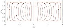
Figure 7: Current distribution in the Ohmic regime obtained by the same procedure as the results for the ballistic and viscous regimes discussed in the main text. Unlike the latter, ohmic flow is potential and thus features no vortices.

References

- [1] A. Tomadin, G. Vignale, M. Polini, A Corbino disk viscometer for 2D quantum electron liquids Phys. Rev. Lett. 113, 235901 (2014)
- [2] A. Principi, G. Vignale, M. Carrega, M. Polini, Bulk and shear viscosities of the two-dimensional electron liquid in a doped graphene sheet Phys. Rev. B 93, 125410 (2016)
- [3] M. Qi, A. Lucas, Distinguishing viscous, ballistic, and diffusive current flows in anisotropic metals, Phys. Rev. B 104 (19), 195106 (2021)
- [4] C. Q. Cook, A. Lucas, Viscometry of electron fluids from symmetry, Phys. Rev. Lett. 127 (17), 176603 (2021)
- [5] D. Valentinis, J. Zaanen, D. van der Marel Propagation of shear stress in strongly interacting metallic Fermi liquids enhances transmission of terahertz radiation Sci. Rep. 11, 7105 (2021)
- [6] D. Valentinis, Optical signatures of shear collective modes in strongly interacting Fermi liquids Phys. Rev. Research 3, 023076 (2021)
- [7] J. Y. Khoo, P.-Y. Chang, F. Pientka, I. Sodemann Quantum paracrystalline shear modes of the electron liquid Phys. Rev. B 102 085437 (2020)
- [8] J. Y. Khoo, F. Pientka, I. Sodemann The universal shear conductivity of Fermi liquids and spinon Fermi surface states and its detection via spin qubit noise magnetometry New J. Phys. 23 113009 (2021)
- [9] L. Levitov, G. Falkovich, Electron viscosity, current vortices and negative nonlocal resistance in graphene. Nat. Phys. 12, 672 (2016).
- [10] D. A. Bandurin, I. Torre, R. Krishna Kumar, M. Ben Shalom, A. Tomadin, A. Principi, G. H. Auton, E. Khestanova, K. S. Novoselov, I. V. Grigorieva, L. A. Ponomarenko, A. K. Geim, M. Polini, Negative local resistance caused by viscous electron backflow in graphene Science 351, 6277, 1055-1058 (2016)
- [11] F. M. D. Pellegrino, I. Torre, A. K. Geim, M. Polini, Electron hydrodynamics dilemma: Whirlpools or no whirlpools, Phys. Rev. B 94, 155414 (2016).
- [12] A. Lucas, K. C. Fong, Hydrodynamics of electrons in graphene 2018 J. Phys.: Condens. Matter 30 053001
- [13] J. A. Sulpizio, L. Ella, A. Rozen, J. Birkbeck, D. J. Perello, D. Dutta, M. Ben-Shalom, T. Taniguchi, K. Watanabe, T. Holder, R. Queiroz, A. Principi, A. Stern, T. Scaffidi, A. K. Geim, S. Ilani, Visualizing Poiseuille flow of hydrodynamic electrons Nature 576, 75-79 (2019)
- [14] M. J. H. Ku, T. X. Zhou, Q. Li, Y. J. Shin, J. K. Shi, C. Burch, L. E. Anderson, A. T. Pierce, Y. Xie, A. Hamo, U. Vool, H. Zhang, F. Casola, T. Taniguchi, K. Watanabe, M. M. Fogler, P. Kim, A. Yacoby, R. L. Walsworth, Imaging viscous flow of the Dirac fluid in graphene Nature 583, 537-541 (2020)
- [15] B. A. Braem, F. M. D. Pellegrino, A. Principi, M. Roosli, C. Gold, S. Hennel, J. V. Koski, M. Berl, W. Dietsche, W. Wegscheider, M. Polini, T. Ihn, and K. Ensslin, Scanning gate microscopy in a viscous electron fluid Phys. Rev. B 98, 241304(R) – Published 21 December 2018
- [16] U. Vool, A. Hamo, G. Varnavides, Y. Wang, T. X. Zhou, N. Kumar, Y. Dovzhenko, Z. Qiu, C. A. C. Garcia, A. T. Pierce, J. Gooth, P. Anikeeva, C. Felser, P. Narang, A. Yacoby, Imaging phonon-mediated hydrodynamic flow in WTe2 Nature Physics 17, 1216-1220 (2021)
- [17] M. Chandra, G. Kataria, D. Sahdev, Quantum Critical Ballistic Transport in Two-Dimensional Fermi Liquids, arXiv:1910.13737
- [18] A. Gupta, J. J. Heremans, G. Kataria, M. Chandra, S. Fallahi, G. C. Gardner, M. J. Manfra, Hydrodynamic and ballistic transport over large length scales in GaAs/AlGaAs, Phys. Rev. Lett. 126, 076803 (2021)
- [19] A. Gupta, J. J. Heremans, G. Kataria, M. Chandra, S. Fallahi, G. C. Gardner, M. J. Manfra, Precision measurement of electron-electron scattering in GaAs/AlGaAs using transverse magnetic focusing, Nature Communications 12, 5048 (2021)
- [20] H. Guo, E. Ilseven, G. Falkovich, L. Levitov, Higher-than-ballistic conduction of viscous electron flows. Proc. Natl Acad. Sci. USA 114, 3068-3073 (2017).
- [21] P. Ledwith, H. Guo, A. Shytov, L. Levitov Tomographic Dynamics and Scale-Dependent Viscosity in 2D Electron Systems, Phys. Rev. Lett. 123, 116601 (2019)
- [22] R. Krishna Kumar, D. A. Bandurin, F. M. D. Pellegrino, Y. Cao, A. Principi, H. Guo, G. H. Auton, M. Ben Shalom, L. A. Ponomarenko, G. Falkovich, K. Watanabe, T. Taniguchi, I. V. Grigorieva, L. S. Levitov, M. Polini, and A. K. Geim, Superballistic flow of viscous electron fluid through graphene constrictions, Nat. Phys. 13, 1182 (2017).
- [23] H. K. Moffatt, Viscous and resistive eddies near a sharp corner, J. Fluid Mech. 18 1-18 (1964)
- [24] M. Semenyakin, G. Falkovich Alternating currents and shear waves in viscous electronics Phys. Rev. B. 97, 8, 085127 (2018)
- [25] H. Guo, Signatures of hydrodynamic transport in an electron system, Thesis, Massachusetts Institute of Technology, Department of Physics, 2018.