Inference of population-level disease transmissibility from household-structured symptom onset data

Abstract

First Few X (FFX) studies collect household-stratified data in the early stages of a pandemic, in order to infer severity and transmissibility of an emerging disease. We present a Bayesian method to approximately infer population-level transmissibility for the first time from such data; previous studies have only inferred household-level transmissibility. To do this we perform the inference at two levels, assuming one transmission rate parameter for within-household infection, and another transmission rate parameter for infection between different households. We use a simplifying assumption: that between-household infections always occur in naive households; while still performing full joint inference on the within-household infection parameters. In addition, a novel technique is used to remove systematic bias when the number of new infections per day is growing or decaying, as is common in real outbreaks, without the need for contemporaneous estimates of the serial interval. The method is validated on simulated data and is shown to perform well, even when the number of infected households is relatively small.

1 Introduction

The threat from pandemics is ongoing [44], and this threat has been underscored by the outbreak of COVID-19 [45]. An important part of dealing with this threat is the ability to infer the characteristics of an emerging strain of infection, in particular its transmissibility and severity, which are strong determinants of impacts of the disease [25, 35, 36].

The accurate inference of transmissibility is particularly challenging, due to the inherently heterogeneous mixing present in larger populations. Models with two levels of mixing, or so-called household models [4, 3], are an established way to capture some of this heterogeneity [18, 37, 17]. These assume stronger mixing within a household, and weaker mixing in the overall population between individuals in different households [4, 37, 7]. Households are a convenient unit to monitor because contacts are easy to track; and although different rates of mixing have been shown to exist within households [29, 14], within-household mixing can be assumed to be homogeneous as a first order approximation.

As one part of the response to the threat of a pandemic, governments around the world have invested in advanced plans for data collection in its early stages, so-called “First Few X”, or FFX, studies [2, 16, 26, 41]. As this data is already at the household level, it is natural to consider its use in the inference of transmissibility in a two-level model of the entire population. Previous work has shown how mechanistic models can be used to accurately infer transmissibility within a household using FFX data [8]. In this paper, we build on this and demonstrate how FFX data can also be used to infer population level transmissibility. The method presented here is effective even if some cases are asymptomatic and hence some infected households are not observed.

The method is a three-step process. The first step, the inference of within-household parameters, uses similar methods to our previous work [8, 6], and so is not described in detail in this paper.

The second step infers the between-household component of transmissibility. This uses the within-household parameters inferred during the first step. By using these inferred within-household parameters, we avoid the need to contemporaneously estimate the generation time or serial interval (for instance via contact tracing), as is used in established methods [11, 39] but has its difficulties.

The third and final step of our method is to combine the within-household and between-household parameters to obtain the posterior distribution of whichever reproduction numbers are desired. Those most commonly reported are $R_{0}$ (the mean number of secondary infections per infectious individual, in an otherwise uninfected population), or $R_{\text{eff}}$ (the mean number of secondary infections per infectious individual, during an outbreak). There is some question over what is the most meaningful way to precisely define $R_{0}$ or $R_{\text{eff}}$ in a two-level model [4, 30, 15], or even whether the between-household reproduction number $R_{*}$ (the mean number of households secondary households infected per infectious household) [37] is a more useful measure of transmissibility. In any case, any of these reproduction numbers can be derived from the within-household and between-household parameters. It is also possible to infer the posterior distribution of the growth rate, which can then be used for forecasting, if exponential growth or decay is assumed [22].

Due to the small amount of FFX data in Australia during the COVID-19 pandemic – partly due to the fortunate situation of there not being a large number of COVID-19 cases – this study uses synthetic data. This use of synthetic data allows us to make a number of simplifying assumptions. We present these assumptions, and the details of the data and model, in Section 2. We outline the method and its theory in Section 3, including two alternative methods in Sections 3.4 and 3.5. We present sample results in Section 4 and a conclusion in Section 5.

2 Data and Model

2.1 Data

For every household which has had a symptomatic infection, the number of individuals in that household is recorded, as well as a daily record of the number of newly symptomatic individuals each day. This corresponds to the Australian pandemic response plan [2], which specifies that this daily data should be obtained from all of the FFX infected households. We assume that every symptomatic case will be detected and recorded and that the day of first symptoms can be accurately determined. We also assume that symptoms always correspond to the disease of interest.

2.2 Model

The model consists of a set of households, each represented by a stochastic compartmental model (Section 2.2.1), with the addition of between-household infection events (Section 2.2.2).

As synthetic data is used, we have made some simplifying assumptions. We assume that there is effectively an infinite supply of naive households, meaning that the spread between households can be approximated as a branching process [42], which is a reasonable assumption in a population containing a large number of households. Following on from this, we also assume that every between-household infection infects a naive household; in other words, that no household contains two or more individuals who have been infected by someone outside of the household.

We also assume that, apart from the initial “seed” infection into a population, there are no further infections from outside the population. This is a less realistic assumption, and the tracing associated with the spread of COVID-19 has shown that populations continually receive external infections, at some rate. Some analyses have this external infection as a separate rate, splitting infection into “local” and “imported” [39]. We ignore this factor, though in principle it would not be difficult to account for it.

2.2.1 Within-household model

The methods in this paper can be adapted to a number of different compartmental household models, but we focus here on a single model to illustrate the methods: a model designed to emulate the progress of a COVID-19 infection. The compartments, which are the possible states of an individual, are illustrated in Figure 1. The process is modelled as a continuous-time Markov chain (CTMC) and the events, rates and parameters are given in Table 1. The model is an extension of the common SEEIIR model with partial observation [8, 28, 33]; in that it has two “pre-symptomatic” compartments to account for the time in which an infected individual is infectious before symptoms appear, as occurs with COVID-19. The model assumes that infectiousness is equal in all of the “infectious” compartments ($P_{1}$, $P_{2}$, $I_{s1}$, $I_{a1}$ and $I_{2}$).

Individuals are symptomatic with probability $p_{s}$, and the $I_{a1}$ compartment denotes cases which are never symptomatic.

Figure 1: Individuals’ compartments in the COVID-19 within-household model. Possible changes in an individual’s compartment are shown as solid or dashed lines, with the only observable change ($P_{2}\rightarrow I_{s1}$) a solid line. Between-household infections are not shown in this diagram.

Description	Transition	Rate	Observed
Exposed to infection	$S\rightarrow E_{1}$	$\beta SI/(m-1)$	no
Exposed state progresses	$E_{1}\rightarrow E_{2}$	$2E_{1}/t_{E}$	no
Becomes infectious, pre-symptomatic	$E_{2}\rightarrow P_{1}$	$2E_{2}/t_{E}$	no
Pre-symptomatic state progresses	$P_{1}\rightarrow P_{2}$	$2P_{1}/t_{P}$	no
Becomes infectious with symptoms	$P_{2}\rightarrow I_{s1}$	$2P_{2}\,p_{s}/t_{P}$	yes
Infectious state progresses	$I_{s1}\rightarrow I_{2}$	$2I_{s1}/t_{I}$	no
Becomes infectious, no symptoms	$P_{2}\rightarrow I_{a1}$	$2P_{2}(1-p_{s})/t_{P}$	no
Infectious state progresses	$I_{a1}\rightarrow I_{2}$	$2I_{a1}/t_{I}$	no
Recovery	$I_{2}\rightarrow R$	$2I_{2}/t_{I}$	no

Table 1: Within-household transition rates for the COVID-19 model. In the “Rate” column, by a slight abuse of notation, the compartment name refers to the number of individuals in that compartment. $\beta$ is the within-household infection rate parameter; $I=(P_{1}+P_{2}+I_{s1}+I_{a1}+I_{2})$ is the total number of infectious individuals in the household; $m$ is the number of individuals in a household; $t_{E}$, $t_{P}$ and $t_{I}$ are the mean times in the exposed (but not infectious), pre-symptomatic (and infectious) and symptomatic states respectively; and $p_{s}$ is the probability of an infectious individual becoming symptomatic.

2.2.2 Between-household model

For the process of between-household infection, we assume that the population of naive (that is, fully susceptible) households is large, so new infections can be modelled as a branching process. Thus the rate at which new households become infected is given by $\alpha$, the rate of between-household infections per infectious individual, multiplied by the total number of infectious individuals (that is, the sum of individuals in the compartments $P_{1}$, $P_{2}$, $I_{s1}$, $I_{a1}$ and $I_{2}$) across all households. As the supply of susceptible households is effectively infinite, this term does not need to be reduced as the outbreak progresses, unlike the within-household infection rate.

Since it is assumed that no household is infected from another household more than once, any newly infected household initially has one individual in the $E_{1}$ compartment, and all other individuals in the $S$ compartment. However the household is not observed, if it is observed at all, until one of the individuals in the household becomes symptomatic; that is, until a $P_{2}\rightarrow I_{s1}$ event occurs for one of the individuals in the household.

3 Method

We infer the reproduction numbers by a three-step process: (1) treat households as independent populations, and infer the within-household model parameters; (2) treat households as units, and infer $\alpha$, the between-household infection rate per infectious individual; and (3) combine the parameters obtained in Steps (1) and (2), to obtain the reproduction numbers. These are described in Sections 3.1, 3.2 and 3.3 respectively.

In addition, we describe two alternative methods in Sections 3.4 and 3.5, which mainly differ at Step (2). The method in Section 3.2 assumes that only data for the first symptomatic infection in each household can be reliably obtained; that is, the data records the day on which each household first has a symptomatic case. The alternative method in Section 3.4 assumes that the day of first symptoms is also available for every individual. This is discussed after Section 3.2 because infector individuals can be treated as households of size $1$, making this in most ways a special case of the method discussed in Section 3.2.

Section 3.5 describes a simpler method which bypasses Step (2), at some cost in accuracy, by first assuming an exponential growth rate $r$, and using that to find the between-household infection rate $\alpha$.

3.1 Step 1: Infer the within-household parameters

The first step of the method is to infer within-household parameters from the FFX data. We use data from within the observed households, and assuming independence between these households, consistent with the assumption of branching dynamics, perform inference and hence sample from the joint posterior distribution for the within-household parameters which were described in Table 1: $\beta$, $t_{E}$, $t_{P}$, $t_{I}$ and $p_{s}$; though instead of $\beta$ we infer $R_{0i}=\beta(t_{P}+t_{I})$, the within-household component of the reproduction number $R_{0}$ or $R_{\text{eff}}$.

This step is essentially the same as described in our previous paper [8], using a Markov chain Monte Carlo scheme to sample from the posterior distribution of the parameters, so it is not described in detail here. The only difference is that instead of an exact matrix exponential approach to calculate the likelihood, we use a particle-marginal approach to estimate the likelihood [43], using importance sampling for the household model [6]. Despite being an estimate, this still targets the correct posterior distribution [38]. This has the advantage of being able to handle more complex household models and larger household sizes.

The output from this step is $N_{S}$ samples from the joint posterior of the within-household parameters. We typically use $N_{S}=10000$, thinning down from a larger number of posterior points obtained during the Markov chain Monte Carlo inference.

Although it is not our direct aim in this paper, we note that the inference of within-household parameters other than the transmission rate provides other valuable information on the epidemic: the time-related parameters ($t_{E}$, $t_{P}$ and $t_{I}$) provide information such as the latent period (time from infection to infectiousness), incubation period (time from infection to symptoms) and infectious period; while $p_{s}$ gives a measure of the severity of the disease; and this all arises due to the collection of FFX data. More detailed information on severity can be obtained if extra FFX data is collected, such as which individuals needed to visit a doctor or hospital.

3.2 Step 2: Infer the between-household infection rate

The second step of inference is to infer $\alpha$, the between-household infection rate per infectious individual, from the daily information of newly infected households. By assuming an effectively infinite supply of households, the spread of infection between households can be modelled as a branching process.

To simplify the discussion, we first consider the case in which all households are the same size (that is, all households contain the same number of individuals), and all households contain at least one symptomatic case. The extensions to different household sizes and households without symptomatic cases, which add several terms to the equations, but are not difficult conceptually, are given in Section 3.2.2.

3.2.1 Fixed household size, all symptomatic

For the purposes of between-household inference, we need only the date of the first symptomatic case in each household. (Section 3.4 describes the situation in which the dates of all individual symptomatic cases in each household are available.) Therefore the data can be condensed to a single vector of daily observations $y=(y_{1}\dots y_{d})$, where each element $y_{j}$ is the number of households which are first symptomatic (that is, having at least one individual in the household showing symptoms, for the first time) on day $j$. The inference method is to estimate $\mathbb{E}[y_{j}]$, the expected number of newly symptomatic households on day $j$, in terms of $\alpha$, and hence estimate the posterior distribution of $\alpha$.

In order to estimate $\mathbb{E}[y_{j}]$, we need to estimate the infection potential of a household: the sum of the infectious times of all infected individuals in that household. Then $\Psi$, the expected value of the infection potential, is given by:

$$\Psi=\mathbb{E}\left[\int_{0}^{\infty}I(t)dt\right],$$ (1)

where $I(t)$ is the number of infectious individuals in a household at time $t$. This means that each household generates, on average, $\alpha\Psi$ between-household infections. The value of $\Psi$ can be estimated from simulations of the household model.

We also need the distributions of $A_{1}$, $A_{2}$ and $G$, as shown in Figure 2. That is, for any given pair of infector and infectee households, we define: $A_{1}$ to be a random variable denoting the time from infection to first symptoms in the infector household (the household-wise equivalent of the incubation period [13]), rounded to the nearest day; $A_{2}$ to be a random variable denoting the time from infection to first symptoms in the infectee household, rounded to the nearest day; and $G$ to be a random variable denoting the time from first infection in the infector household to first infection in the infectee household (the household-wise equivalent of the generation time [9]), rounded to the nearest day. We also define $S_{H}$ to be a random variable denoting the time from first symptoms in the infector household to first symptoms in the infectee household (the household-wise equivalent of the serial interval [12]); and $C$ to be the sum of $G$ and $A_{2}$, making it the time from first infection of the infector household, to first symptoms in the infectee household, rounded to the nearest day.

Figure 2: Schematic representation of the random variables $A_{1}$, $A_{2}$, $G$, $S_{H}$ and $C$. Time progresses from left to right, and each square represents a day. “E” denotes the day a household is first exposed and infected; and “FS” denotes the first day of symptoms in a household. A dotted line is used to show $S_{H}$, the household-wise equivalent of the serial interval, because it is discussed but not used. The bottom row shows the dummy variables used for each day in the analyses in Sections 3.2 and 3.4.

An important part of our method is that, for a given sample of the within-household parameters, we can obtain unbiased estimates for the distributions of $A_{1}$, $A_{2}$ and $G$ (and hence $C$) from simulation of the within-household model, without the need for contact tracing.

The analysis would be simpler if we could use $S_{H}$, the household-wise equivalent of the serial interval, to estimate $\mathbb{E}[y_{j}]$. However an unbiased distribution of $S_{H}$ cannot be obtained without accounting for the growth or decay in the outbreak [10], in terms of the number of newly infected households per day. This is because a sample of $S_{H}$ is obtained by subtracting a sample of $A_{1}$ from a sample of $C$; and this subtraction of $A_{1}$, also referred to as looking backwards in time [9], biases the distribution depending on whether the outbreak is growing or decaying, as has been pointed out previously [40, 9, 10].

However it is possible to estimate $\mathbb{E}[y_{j}]$ without $S_{H}$ and without contact tracing, using the other variables in Figure 2, because these are estimated forward from the day the infector household is exposed (day $l$ in Figure 2). To do this, it is useful to define $w_{(j,k,l)}$, the expected number of between-household infections which are caused by an infector household which was infected on day $l$ and first symptomatic on day $k$, and which are first symptomatic in an infectee household on day $j$. Then consideration of each day $j$ gives:

$$\mathbb{E}[y_{j}]=\sum_{k}\sum_{l}w_{(j,k,l)}.$$ (2)

Since every infector household generates on average $\alpha\Psi$ between-household infections, it follows from consideration of each day $k$:

$$\alpha\Psi\mathbb{E}[y_{k}]=\sum_{j}\sum_{l}w_{(j,k,l)};$$ (3)

and considering infections generated from households initially infected on day $l$ gives:

$$w_{(j,k,l)}=\alpha\Psi T_{l}\,p(A_{1}=k-l,C=j-l),$$ (4)

where $T_{l}$ is the true number of households infected on day $l$. We cannot measure $T_{l}$, but a reasonable approximation is that it is proportional to $y_{l}$, as this would be the case if the rate of growth or decay was constant and if there was no stochasticity. So we estimate $T_{l}$ to be $y_{l}$ multiplied by some value $K_{k}$ which is constant for each value of $k$, giving:

$$w_{(j,k,l)}=\alpha\Psi y_{l}K_{k}\,p(A_{1}=k-l,C=j-l).$$ (5)

We estimate $K_{k}$ by substituting (5) into (3) and replacing $\mathbb{E}[y_{k}]$ with the observed value $y_{k}$, giving:

$$\alpha\Psi y_{k}=\sum_{j}\sum_{l}\alpha\Psi y_{l}K_{k}\,p(A_{1}=k-l,C=j-l),$$

$$\Rightarrow K_{k}=\frac{y_{k}}{\sum_{j}\sum_{l}y_{l}\,p(A_{1}=k-l,C=j-l)}.$$ (6)

Since all days $l$ will be the same as or earlier than day $k$, it follows that $K_{k}>1$ when the number of new infections per day is growing at day $k$, $K_{k}<1$ when it is falling, and $K_{k}\approx 1$ when it is approximately constant. So the $K_{k}$ factor provides a correction to account for the growth or decay of the outbreak. Appendix B illustrates how inference results can be biased if this term is not included.

Then substituting (5) into (2) gives:

$$\mathbb{E}[y_{j}]=\alpha\Psi\sum_{k}\sum_{l}y_{l}K_{k}\,p(A_{1}=k-l,C=j-l).$$

As shorthand, we define the quantity $\xi_{j}$ which is equal to $\mathbb{E}[y_{j}]/\alpha$, that is:

$$\xi_{j}=\Psi\sum_{k}\sum_{l}y_{l}K_{k}\,p(A_{1}=k-l,C=j-l).$$ (7)

We use a gamma distribution as the prior of $\alpha$, meaning that if the data is Poisson distributed, then the posterior distribution of $\alpha$ is also a gamma distribution [11, 39]. Using $c$ days of data up to and including day $d$, it can be shown (Appendix A) that the posterior of $\alpha$ is

$$f(\alpha|y)\sim\text{Gamma}\left(a+\sum_{j=d+1-c}^{d}y_{j},\quad b+\sum_{j=d+1-c}^{d}\xi_{j}\right),$$ (8)

where the first parameter is the shape and the second parameter is the rate, and $a$ and $b$ are the prior’s shape and rate respectively. This equation gives the distribution of $\alpha$ as calculated on day $d$.

Aside from the observed data values in $y$, all quantities on the right hand sides of (6) and (7) can be estimated from simulations of the household model. Thus this step gives samples from the joint posterior distribution of $\alpha$ and the within-household parameters.

By making $K_{k}$ constant for any value of $k$, we are assuming a constant rate of growth or decay. A more sophisticated calculation may be possible which accounts for change in this rate. But since we are only using the last $c$ days of data for inference in (8), this should not be necessary. However, it may be a point for investigation in the future.

3.2.2 General case

We modify the discussion in the previous section to account for households of different sizes, and asymptomatic cases.

To account for asymptomatic cases, we define $p_{h}$ to be the probability of an infected household being symptomatic, and $p_{i}$ to be the probability of a randomly chosen infectious individual being a member of a symptomatic household. We define a symptomatic household to be an infected household in which at least one individual is eventually symptomatic; and an asymptomatic household to be an infected household in which all infected individuals remain asymptomatic.

To account for different household sizes, we require the observed data to be a 2-dimensional array $y$, with $y_{(j,n)}$ being the number of households of size $n$ which are first symptomatic on day $j$. We replace $\Psi$ with $\Psi_{m}$, the expected infection potential of a symptomatic household of size $m$, given by:

$$\Psi_{m}=\mathbb{E}\left[\int_{0}^{\infty}I_{m}(t)dt\right],$$ (9)

where $I_{m}(t)$ is the number of infectious individuals in a symptomatic household of size $m$ at time $t$. In addition, $M$ and $N$ are random variables denoting the sizes of the infector and infectee households respectively.

We define the quantity $w_{(j,k,l,m,n)}$, which is the expected number of between-household infections which are caused by an infector household of size $m$ which was infected on day $l$ and first symptomatic on day $k$, and which are first symptomatic in an infectee household of size $n$ on day $j$.

Then consideration of each day $j$ also needs to account for the fact that on average only $p_{i}$ of all infections come from infectious households, and only $p_{h}$ of infections are in infectee households which become symptomatic. So (2), (3) and (4) are modified to:

$$\mathbb{E}[y_{(j,n)}]=\frac{p_{h}}{p_{i}}\sum_{k}\sum_{l}\sum_{m}w_{(j,k,l,m,n)};$$ (10)

$$\alpha\Psi_{m}\mathbb{E}[y_{(k,m)}]=\sum_{j}\sum_{l}\sum_{n}w_{(j,k,l,m,n)};\text{ and}$$ (11)

$$w_{(j,k,l,m,n)}=\alpha\Psi_{m}T_{l,m}\,p^{*}(A_{1}=k-l,C=j-l,N=n|M=m);$$ (12)

where $T_{(l,m)}$ is the true number of symptomatic households of size $m$ infected on day $l$, and $p^{*}$ means “the probability, given that both the infector and infectee households are symptomatic”.

Then following a similar analysis to Section 3.2.1 gives:

$$K_{(k,m)}=\frac{y_{(k,m)}}{y_{(l,m)}\,p^{*}(A_{1}=k-l,C=j-l,N=n|M=m)}$$ (13)

and

$$\xi_{(j,n)}=\frac{p_{h}}{p_{i}}\sum_{k}\sum_{l}\sum_{m}\Psi_{m}y_{(l,m)}K_{(k,m)}\,p^{*}(A_{1}=k-l,C=j-l,N=n|M=m),$$ (14)

where $\xi_{(j,n)}=\mathbb{E}[y_{(j,n)}]/\alpha$.

We again use a gamma distribution as the prior of $\alpha$, and infer using $c$ days of data up to and including day $d$. This means (8) is modified to:

$$f(\alpha|y)\sim\text{Gamma}\left(a+\sum_{j=d+1-c}^{d}\sum_{n}y_{(j,n)},\quad b+\sum_{j=d+1-c}^{d}\sum_{n}\xi_{(j,n)}\right),$$ (15)

where the first parameter is the shape and the second parameter is the rate, and $a$ and $b$ are the prior’s shape and rate respectively.

Once again, aside from the observed data values in $y$, all quantities on the right hand sides of (13) and (14) can be estimated from simulations of the household model. Therefore, for each of the $N_{S}$ samples from the joint posterior of the within-household parameters obtained in Step 1, we run a number of simulations of the household model (typically 1000) per household size, allowing $\xi_{(j,n)}$ to be estimated for all values of $n$, for each day $j$; and then a single sample of $\alpha$ is taken from (15). Thus this step gives $N_{S}$ samples from the joint posterior distribution of $\alpha$ and the within-household parameters.

3.3 Step 3: Calculating reproduction numbers and growth rate

Once samples of all the model parameters are obtained, the population reproduction numbers are fairly straightforward to evaluate.

To account for different household sizes, we define $h_{m}$ to be the probability that a randomly chosen household will be of size $m$. Therefore a newly infected household has size $m$ with probability $\pi_{m}$, where $\pi_{m}$ is the size-biased distribution [7], and is given by the equation,

$$\pi_{m}=\frac{mh_{m}}{\sum_{i}ih_{i}}.$$ (16)

The household reproduction number $R_{*}$ [7] can then be evaluated using previously obtained values:

$$R_{*}=\alpha\sum_{m}\pi_{m}\Psi_{m},$$ (17)

where $\Psi_{m}$ is given in (9).

We use the definition of $R_{0}$ as the expected number of infections directly caused by the very first infectious individual in the population. For each value of the household size $m$, one can run simulations of the household model and estimate $g_{m}$, the mean number of infections caused directly by the first infected member of the household, giving:

$$R_{0}=\sum_{m}\pi_{m}g_{m}.$$ (18)

This equation can also be used to calculate $R_{\text{eff}}$.

Other definitions of $R_{0}$ and $R_{\text{eff}}$ have been proposed for two-level models [4, 15, 30]. These can also be calculated using the raw data from the previous steps. For instance, an alternative might be to use $R_{HI}$ [15], the expected number infected by a randomly chosen infectious individual. In that case, we estimate $f_{m}$, the average number of infections within an infected household of size $m$, from simulations of the household model. Between them, the $f_{m}$ household members generate on average $(f_{m}-1)$ within-household infections and $\alpha\Psi_{m}$ between-household infections, giving:

$$R_{HI}=\sum_{m}\pi_{m}\frac{f_{m}-1+\alpha\Psi_{m}}{f_{m}}.$$ (19)

An estimate of the exponential growth rate $r$ can also be obtained [7], by finding the value of $r$ for which

$$\alpha\sum_{m}\pi_{m}\mathbb{E}\left[\int_{0}^{\infty}I_{m}(t)e^{-rt}dt\right]=1.$$ (20)

Equation (20) includes a path integral, and its expectation can be calculated by solving a set of linear equations [32, 31, 37], which are written in terms of the generator of the within-household CTMC. However this has a practical drawback: the calculations each require a square matrix with one row and one column for each non-absorbing state of the household model, and so the size of such matrices increases exponentially with the household size $m$. In our experience these matrices get infeasibly large, in terms of computer memory and execution time, for $m$ over $8$ or so household members.

A simpler and more practical approach is to also estimate this quantity with the aid of simulation. Any simulation of $I_{m}(t)$ is a piecewise step function, meaning $\int_{0}^{\infty}I_{m}(t)e^{-rt}dt$, and hence the left hand side of (20), can be efficiently estimated by simulation for any given value of $r$; allowing $r$ to be found using a root finding program [1]. The simulations are not memory-intensive and so do not have the same limitations as the system of linear equations method. Another advantage is that, by incorporating the summation into an existing simulation model, the code is relatively easy to verify.

In all cases, these parameters are evaluated as samples from the distribution of the posterior. The output from Step (2) is $N_{S}$ samples from the joint posterior of $\alpha$ and the within-household parameters; we typically use $N_{S}=10000$. The method in Step (3), to evaluate any of $R_{*}$, $R_{0}$, $R_{\text{eff}}$ or $r$, is repeated for each of these samples. Therefore the method gives $N_{S}$ joint samples of all parameters.

3.4 Observed individuals

In this section and in Section 3.5, we present two alternate methods, which are relevant if different data is available.

The analysis in Section 3.2 assumes that the only observed data is the number of newly symptomatic households of each household size on each day, which is stored in the 2-dimensional array $y$. In this section we consider the situation in which the number of newly symptomatic individuals is also available. We denote this as $z=(z_{1}\dots z_{d})$, where $z_{j}$ is the number of individuals who are first symptomatic on day $j$.

In that case, there is no need to use the infector households to estimate the number of newly infectious individuals, because that quantity is available directly as $z$. The two-dimensional array $y$ is still used as the count of new infectee households.

Infector individuals can be treated identically to infector households of size $1$, which are symptomatic with probability $p_{s}$ (Table 1). So we modify the analysis of Section 3.2.2 by replacing $y_{(l,m)}$ with $z_{l}$ for all $l$, replacing $y_{(k,m)}$ with $z_{k}$ for all $k$, setting $m=1$ as the only possible value of $M$, and replacing $p_{i}$ with $p_{s}$. This means (13) is modified to:

$$K_{(k,1)}=\frac{z_{k}}{\sum_{j}\sum_{l}\sum_{n}z_{l}\,p^{*}(A_{1}=k-l,C=j-l,N=n|M=1)};$$ (21)

and (14) is modified to:

$$\xi_{(j,n)}=\frac{p_{h}}{p_{s}}\sum_{k}\sum_{l}\Psi_{1}z_{l}K_{(k,1)}\,p^{*}(A_{1}=k-l,C=j-l,N=n|M=1).$$ (22)

The rest of the analysis proceeds as in Sections 3.2.2 and 3.3, including the use of (15) to find the distribution of $\alpha$.

3.5 Inferring $r$ directly, and $\alpha$ from $r$

Another alternative method, which builds on a previously published method [37, 7], is to first infer the growth rate $r$, and then use $r$ to find $\alpha$. This estimate of $\alpha$, along with the estimates of the within-household parameters obtained in Step 1, is then used to obtain estimates of $R_{*}$, $R_{0}$ or $R_{\text{eff}}$. The inference of $r$ is an extra step in this inference, so this method is usually not preferred. However it might be preferable in situations where the exponential growth rate is relatively easy to obtain. For instance, the distribution of $r$ could be approximately inferred by performing a Bayesian linear regression of log$(y)$ versus time, where $y$ is the number of newly infected households per day.

Given samples from the posterior distribution of $r$ obtained by this or another method, we can take samples from the posterior of the within-household parameters, and calculate corresponding samples of the between-household infection rate $\alpha$ using (20), but with $\alpha$ rather than $r$ being the unknown quantity. As in Section 3.3, usually the simplest and most efficient way to find $\alpha$ is to estimate the integral in (20) by simulation.

With samples of $\alpha$ generated, corresponding samples of $R_{*}$, $R_{0}$ or $R_{\text{eff}}$ can then be generated using (17), (18) or (19) as appropriate.

This method has the appeal of bypassing the Section 3.2 calculation of $\alpha$. However a disadvantage is that the samples of $r$ are not joint with the samples of the within-household parameters. This is likely to contribute to an overestimation in the variances in the distributions of $\alpha$, $R_{*}$, $R_{0}$ and $R_{\text{eff}}$.

4 Testing and Results

For the first two sets of tests, in Figure 3 and 4, data was generated using the parameters: $t_{E}=2$, $t_{P}=1.8$, $t_{I}=1.5$, $p_{s}=0.8$, $R_{0i}=\beta(t_{P}+t_{I})=1.4$; and $\alpha$ initially $0.242$, then reducing to $0.121$ on day $70$. For $h_{m}$, the proportions of households of size $m$, and hence the values of the size-biased distribution $\pi_{m}$ (Section 3.3), we used household size data from the 2016 Australian Census [20], capped at a size of 6, as shown in Table 2.

$m$	number of households	$h_{m}$	$\pi_{m}$
1	2023537	0.244	0.095
2	2768286	0.334	0.260
3	1338376	0.162	0.188
4	1313551	0.159	0.246
5	557262	0.067	0.131
6	284067	0.034	0.080

Table 2: Household size data, from the 2016 Australian Census [20], capped at a size of 6. $h_{m}$ is the proportion of households which are of size $m$, while $\pi_{m}$ is the proportion of individuals who live in a household of size $m$. These values of $h_{m}$ and $\pi_{m}$ are used throughout the tests in this section.

Inference was performed using the method described in Sections 3.1 to 3.3, using (18) to evaluate $R_{\text{eff}}$ and (17) to evaluate $R_{*}$. (All tests were repeated using the method in described in Section 3.4, with very similar results). The following priors were used for the within-household parameters: $R_{0i}$ had a gamma distribution with shape $3$ and rate $5/3$ (mean = $1.8$); $t_{E}$ had a gamma distribution with shape $3$ and rate $0.5$ (mean=$6$); $t_{P}$ and $t_{I}$ both had a gamma distribution with shape $3$ and rate $2$ (mean=$1.5$); and the prior for $p_{s}$ had a beta distribution with $\alpha=2.8$ and $\beta=1.2$ (mean=$0.7$). For the between-household infection parameter $\alpha$, we followed previous work [39] and chose a fairly broad prior: a gamma distribution with shape $1$ and scale $0.3$ (mean=$0.3$). With a prior mean infectious time ($t_{P}+t_{I}$) of $3$, this corresponds to a mean of $0.9$ for the between-household component of $R_{\text{eff}}$.

For the first set of tests, we ran the within-household inference only once, inferring the within-household parameters from the full FFX data for the first $50$ households, but used daily updates of data for the between-household inference. This was partly a decision of practicality: the between-household inference is far faster to run than the within-household inference, due to the former’s use of conjugate priors. It also reflects the authors’ experience of FFX data collection in Australia during the COVID-19 outbreak, in which updates of within-household data tended to occur slowly. But it is also based on a reasonable assumption: that as countermeasures such as social distancing and working from home are brought in to restrict an outbreak, primarily the between-household infection rate will be affected, and the within-household parameters will be impacted less.

We performed inference of $R_{\text{eff}}$ and $R_{*}$ for each day of the simulated outbreak, using the most recent $7$ days of data for the between-household inference, and the results are shown in Figure 3. It shows that inference works well, even with only $50$ households of FFX data for within-household inference: it tracks changes to the transmission rate, and the confidence interval reduces as the amount of data grows.

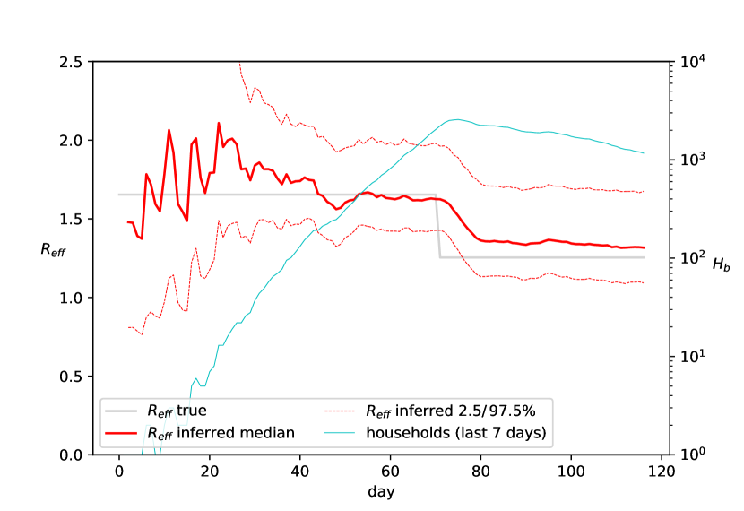
(a)

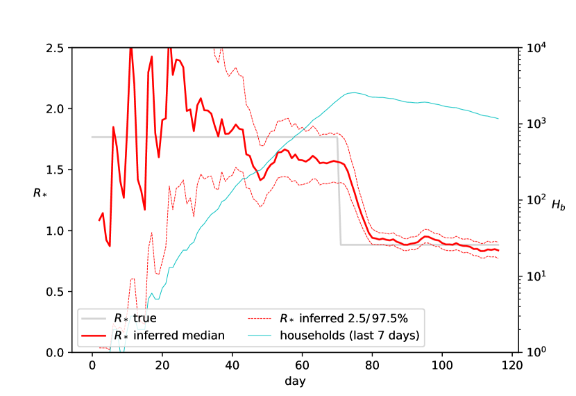
(b)

Figure 3: Inference of (a) $R_{\text{eff}}$ and (b) $R_{*}$ during a simulated outbreak: between-household inference updated daily, using the most recent $7$ days of data; within-household parameters inferred from 50 households’ FFX data. The dotted red lines show the $2.5$ and $97.5$ percentiles of the posterior; the true value of $R_{\text{eff}}$ or $R_{*}$ is shown in grey; and the number of households infected in the most recent 7 days ($H_{b}$) is shown in light blue.

In order to determine whether the within-household or between-household inference was the main source of variance, the inference was repeated with the within-household parameter values perfectly known (that is, every sample uses the within-household parameters values used to generate the data: $R_{0i}=1.4$, $t_{E}=2$, $t_{P}=1.8$, $t_{I}=1.5$ and $p_{s}=0.8$), with the results in Figure 4.

This shows a substantial reduction in variance, although this is much more pronounced in $R_{\text{eff}}$ than $R_{*}$. This is because $R_{\text{eff}}$, by its very definition in (18) has a substantial within-household component: within-household and between-household infections are counted. In contrast, the evaluation of $R_{*}$ only directly considers between-household transmission, so changes to the within-household inference method have a less dramatic effect on $R_{*}$.

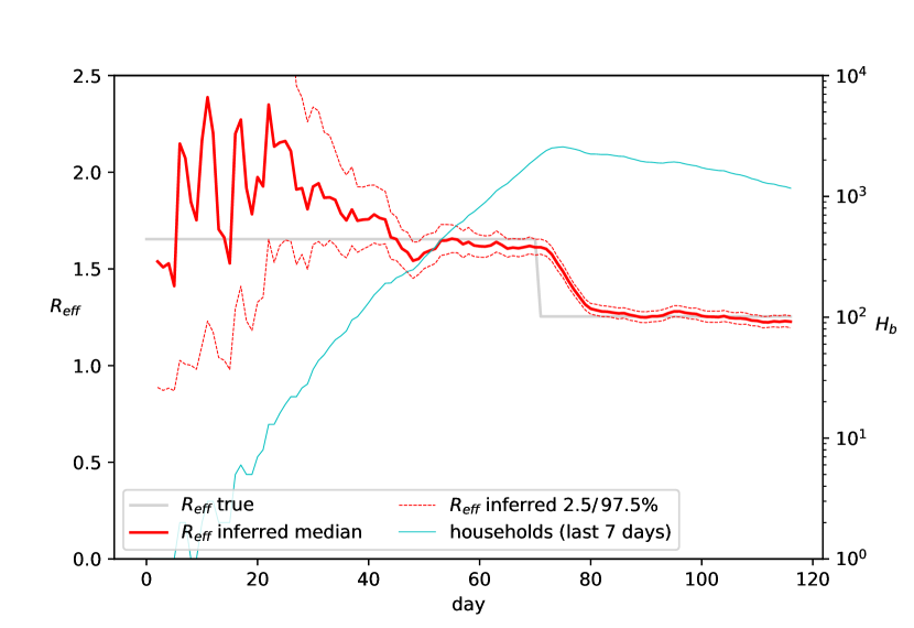
(a)

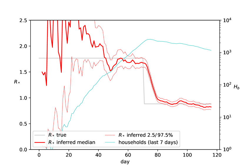
(b)

Figure 4: Inference of (a) $R_{\text{eff}}$ and (b) $R_{*}$ during a simulated outbreak: between-household inference updated daily, using the most recent $7$ days of data; and the within-household parameters known exactly. The dotted red lines show the $2.5$ and $97.5$ percentiles of the posterior; the true value of $R_{\text{eff}}$ or $R_{*}$ is shown in grey; and the number of households infected in the most recent 7 days ($H_{b}$) is shown in light blue.

We tested the method further by aggregating the results from 40 different realisations, across a range of values of $H_{w}$ (the number of households used for within-household inference) and $H_{b}$ (the number of households used for between-household inference), with the results shown in Figure 5. Each of the 40 realisations was generated using the parameters: $R_{0i}=1.4$, $t_{E}=2$, $t_{P}=1.8$, $t_{I}=1.5$, $p_{s}=0.8$, $\alpha=0.242$ and the distribution of household sizes in Table 2; corresponding to $R_{\text{eff}}=1.654$ and $R_{*}=1.766$. As in Figures 3 and 4, the parameter $H_{b}$ refers to the number of houses newly infected in the most recent 7 days. For within-household inference, we also included the results assuming the within-household parameters are known exactly, effectively corresponding to $H_{w}=\infty$.

Overall, these results show that the inference method works well. We see that accuracy improves, and variance decreases, as more data becomes available; and that this is the case for both within-household and between-household inference. This is similar to what is observed in Figures 3 and 4. We also see that one or other component can dominate the variance. That is, if $H_{w}$ is small, there is not a lot to be gained by increasing $H_{b}$; and vice versa.

We do notice that both $R_{\text{eff}}$ and $R_{*}$ are overestimated when there is a small amount of data, in particular for lower values of $H_{b}$. In the case of lower values of $H_{b}$, we believe that the main cause is that the initial fade-out of some realisations causes a “selection bias”, leading to an overestimation of $R_{\text{eff}}$ and $R_{*}$ [27, 34], which is not simple to correct.

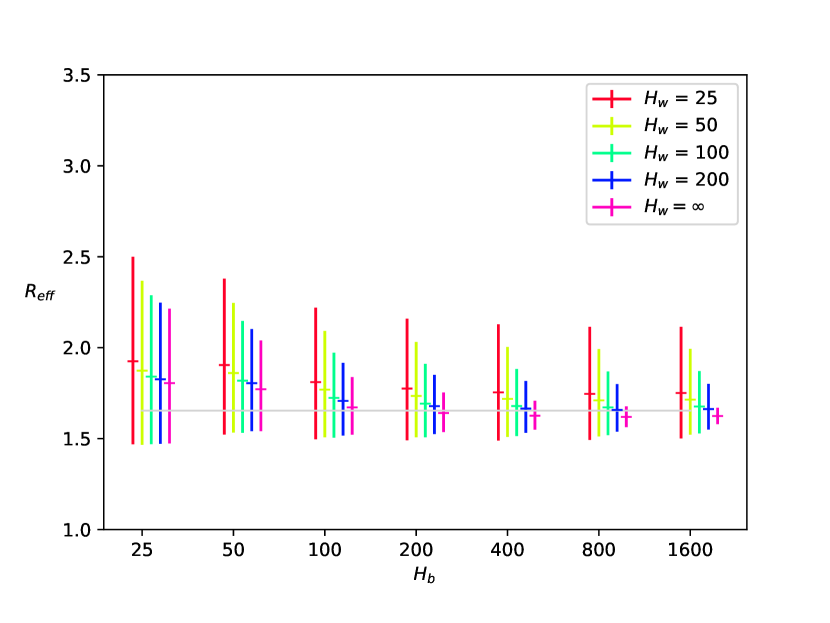
(a)

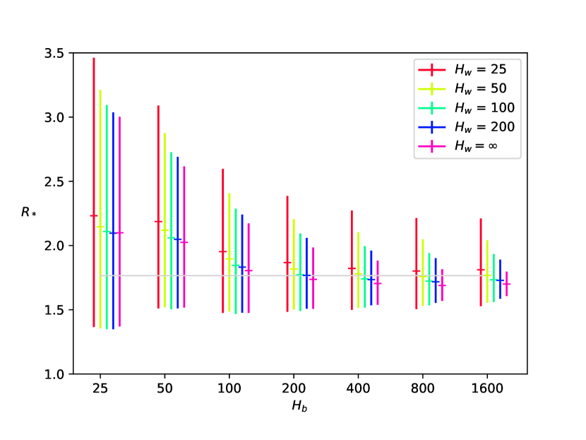
(b)

Figure 5: Plots illustrating the mean and distribution of the posterior of (a) $R_{\text{eff}}$ and (b) $R_{*}$, averaged over the inference results of 40 realisations, for different values of $H_{w}$ (numbers of households used for within-household inference, with $H_{w}=\infty$ meaning the within-household parameters are known exactly) and $H_{b}$ (numbers of households used for between-household inference). The horizontal lines show the means of the 40 posterior distributions, while the lower and upper extremities show the means of the posterior distributions’ $2.5$ percentiles, and the means of the posterior distributions’ $97.5$ percentiles, respectively. The true values ($1.654$ and $1.766$ respectively) are shown as grey lines.

4.1 Forecasting

The inferred values of the exponential growth rate $r$ can also be used for simple forecasting, assuming a continued exponential growth or decay.

In addition to forecasting with the inferred parameters for a given day, forecasts may account for reduced infection rates, re-calculating $r$ using the method in Section 3.3. An example is shown in Figure 6. The true (simulated) progress of the outbreak for the next 10 days is also included, showing that the exponential approximation works reasonably well for a short-term forecast.

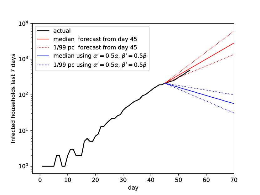
Figure 6: Sample forecasting results, with alternate forecast showing the effect of reducing both the between-household transmission rate $\alpha$, and the within-household transmission rate parameter $\beta$.

5 Conclusion

We have presented a method for inference of infection parameters in a two-level infection model, with different infection rates within households and between different households. By separating the parameters into two components, we split a complicated inference problem into two relatively well understood problems.

The within-household infection parameters can be inferred using known techniques such as a particle-marginal Metropolis-Hastings algorithm [38, 43]. The inferred within-household parameters can then be used to estimate the effective number of infector households on a given day, and hence estimate $\alpha$, the between-household infection rate. The technique is similar to other methods which infer the parameters dynamically during an outbreak [11, 39], but also uses knowledge of within-household structure and parameters, and uses it to eliminate a systematic bias when the number of new infections per day is changing.

The within-household and between-household parameters can be combined, to give the reproduction number in a number of forms. An exponential growth rate $r$ can also be estimated, and used for forecasting. In this case, the required path integral can be efficiently estimated using simulation. In all cases, the testing confirms that the method works well.

This work could be extended in a number of directions. First, we emphasise that the method is not specific to any particular within-household model, so can be adapted to a model for a different type of pathogen, or a more or less detailed model of the internal structure of a household. Also, the method scales well to the use of larger household groups; unlike earlier methods [37, 7] which strained computer resources as household sizes reached even a moderate size.

For the between-household inference, we believe a household-based model can be useful for estimating the spread of an infection through a population. Our technique for overcoming the bias when the number of new infections per day is growing or decaying (Section 3.2) is not limited to a household-based model, so may be applicable in other situations. The technique presented here assumes a constant rate of change, and it may also be useful to refine this technique to account for changes in the rate of growth or decay.

There is also scope for extending the method for forecasting. We present a very simple method, of calculating the exponential growth rate and using that to project forward. But with all lower-level parameters inferred, such as those relating to transmission of the infection and recovery of individuals, it may be possible to make forecasts using those parameters directly, without assuming a constant exponential growth rate.

In conclusion, we believe the stratification of data into households is an effective method for inference of outbreak parameters, and there is much scope for using these or similar methods in the future.

6 Declaration of Competing Interest

The authors declare that they have no known competing financial interests or personal relationships that could have appeared to influence the work reported in this paper.

7 Acknowledgements

This material is based upon work supported by the U.S. Army International Technology Center Pacific (ITC-PAC) under Contract No. FA5209-17-C-0008.

This work was also funded by the Australian Defence Science and Technology Group Bioterrorism Preparedness Strategic Research Initiative 17/491.

This work was supported with supercomputing resources provided by the Phoenix HPC service at the University of Adelaide.

Simulation and inference software was written in Julia [5], with post-processing in Python and Matplotlib [19].

8 References

Appendices

Appendix A Conjugate prior proof

Consider a set of event rates $\alpha\xi_{1}\dots\alpha\xi_{c}$, where $\xi_{1}\dots\xi_{c}$ are known but $\alpha$ is not known; and corresponding observed daily event counts $y=(y_{1}\dots y_{c})$. Given that the prior distribution of $\alpha$ is a gamma distribution with shape $a$ and rate $b$, meaning

$$f(\alpha)=\frac{b^{a}}{\Gamma(a)}\alpha^{a-1}e^{-b\alpha},$$ (23)

we wish to infer the posterior distribution $f(\alpha|y)$.

The number of daily events $Y_{j}$ is poisson distributed, with:

$$p(Y_{j}=y_{j}|\alpha)=\frac{\left(\alpha\,\xi_{j}\right)^{y_{j}}e^{\left(-\alpha\,\xi_{j}\right)}}{y_{j}!};$$ (24)

which means the likelihood $f(y|\alpha)$ is given by:

$$f(y|\alpha)=\prod_{j=1}^{c}p(Y_{j}=y_{j}|\alpha)=\prod_{j=1}^{c}\frac{\left(\alpha\,\xi_{j}\right)^{y_{j}}e^{\left(-\alpha\,\xi_{j}\right)}}{y_{j}!}$$

$$=\frac{\prod_{j=1}^{c}{\xi_{j}}^{y_{j}}}{\prod_{j=1}^{c}y_{j}!}\alpha^{\left(\sum_{j=1}^{c}y_{j}\right)}e^{-\alpha\left(\sum_{j=1}^{c}\xi_{j}\right)}.$$ (25)

Substituting (23) and (25) into Bayes’ rule, noting $\alpha>0$, gives:

$$f(\alpha|y)=\frac{f(y|\alpha)f(\alpha)}{\int_{0}^{\infty}f(y|\alpha)f(\alpha)d\alpha}$$

$$=\frac{\frac{b^{a}\prod_{j=1}^{c}{\xi_{j}}^{y_{j}}}{\Gamma(a)\prod_{j=1}^{c}y_{j}!}\alpha^{(a-1+\sum_{j=1}^{c}y_{j})}e^{-\alpha(b+\sum_{j=1}^{c}\xi_{j})}}{\int_{0}^{\infty}\frac{b^{a}\prod_{j=1}^{c}{\xi_{j}}^{y_{j}}}{\Gamma(a)\prod_{j=1}^{c}y_{j}!}\alpha^{(a-1+\sum_{j=1}^{c}y_{j})}e^{-\alpha(b+\sum_{j=1}^{c}\xi_{j})}d\alpha}.$$

To simplify the logic, we define

$$S=a+\sum_{j=1}^{c}y_{j}\quad\text{ and }\quad R=b+\sum_{j=1}^{c}\xi_{j},$$ (26)

giving:

$$f(\alpha|y)=\frac{\alpha^{S-1}e^{-R\alpha}}{\int_{0}^{\infty}\alpha^{S-1}e^{-R\alpha}d\alpha}$$

$$=\frac{\frac{R^{S}}{\Gamma(S)}\alpha^{S-1}e^{-R\alpha}}{\int_{0}^{\infty}\frac{R^{S}}{\Gamma(S)}\alpha^{S-1}e^{-R\alpha}d\alpha}.$$ (27)

The quantity inside the integral in (27) is a gamma distribution, meaning it integrates to $1$, giving:

$$f(\alpha|y)=\frac{R^{S}}{\Gamma(S)}\alpha^{S-1}e^{-R\alpha},$$

which is itself a gamma distribution, with shape $S$ and rate $R$; that is:

$$f(\alpha|y)\sim\text{Gamma}\left(\text{shape}=a+\sum_{j=1}^{c}y_{j},\quad\text{rate}=b+\sum_{j=1}^{c}\xi_{j}\right).$$ (28)

which is equivalent to (8).

Appendix B Inference during growth and decay

This appendix concerns the correction to account for the growth or decay of an outbreak, which is discussed in Section 3.2.1, and appears as the $K$ term in (7), (14) and (22). We illustrate how, without this term, we see a bias due to the growth or decay of the outbreak, as has previously been reported [40, 9, 10]; and that this $K$ term provides an appropriate correction.

Figures 7 and 8 show inference results, of $R_{\text{eff}}$ and $R_{*}$ respectively, from the same simulation. This simulation uses the distribution of household sizes given in Table 2; within-household parameters $t_{E}=2$, $t_{P}=1.8$, $t_{I}=1.5$, $p_{s}=0.8$, $R_{0i}=\beta(t_{P}+t_{I})=1.4$; and $\alpha$ initially $0.242$, then reducing to $0.0727$ on day $70$. For inference, the within-household parameters are assumed to be known exactly, while $\alpha$ has a gamma distribution with shape $1$ and scale $0.3$. That is, all parameters and settings are identical to those used for Figure 4, except that $\alpha$ reduces more sharply, to exaggerate the rate of decay of $R_{\text{eff}}$ and $R_{*}$.

Without the correction of the $K$ term, the inference method overestimates $\alpha$ when the outbreak is growing, and underestimates $\alpha$ when the outbreak is decaying, causing bias in $R_{\text{eff}}$ (Figure 7(a)) and $R_{*}$ (Figure 8(a)).

When the $K$ term is included, the inference accounts for this growth and decay, as is illustrated in Figures 7(b) and Figure 8(b) respectively.

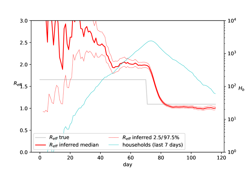
(a) without correction

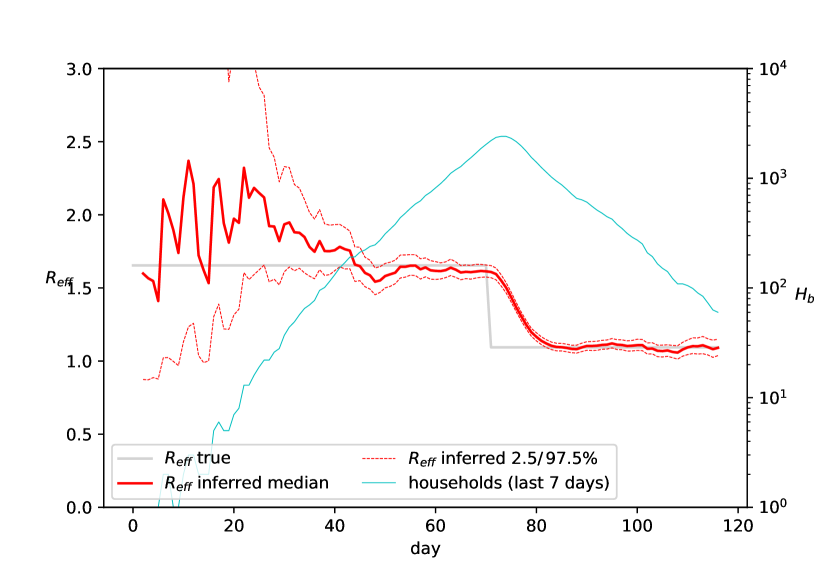
(b) with correction

Figure 7: Inference of $R_{\text{eff}}$ during a simulated outbreak between-household inference updated daily, using the most recent $7$ days of data; and the within-household parameters known exactly. Sub-figure (a) omits the correction due to growth or decay, by setting $K_{(k,m)}=1$ in place of (13). Sub-figure (b) uses the method discussed in the text. The dotted red lines show the $2.5$ and $97.5$ percentiles of the posterior; the true value of $R_{\text{eff}}$ is shown in grey; and the number of households infected in the most recent 7 days ($H_{b}$) is shown in light blue.

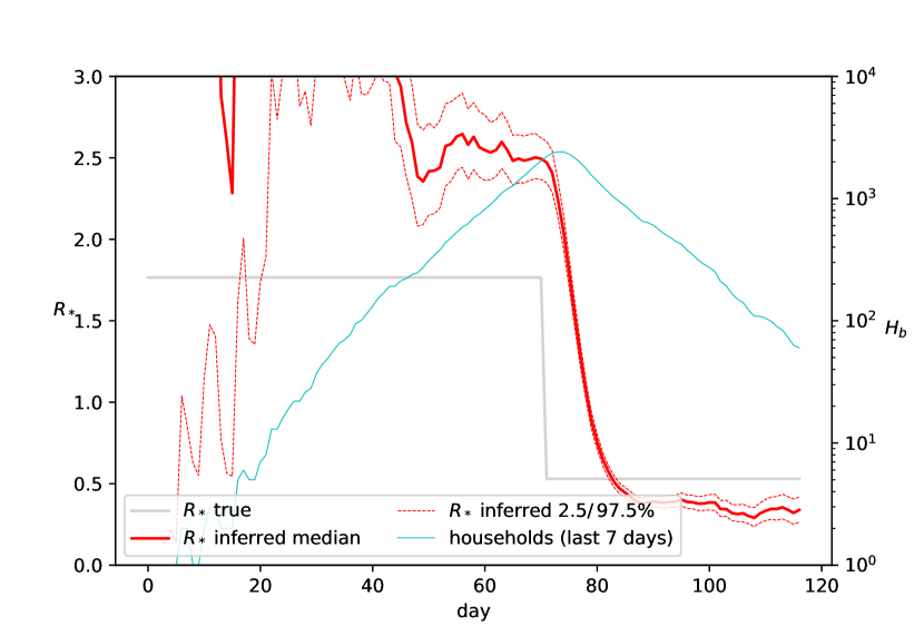
(a) without correction

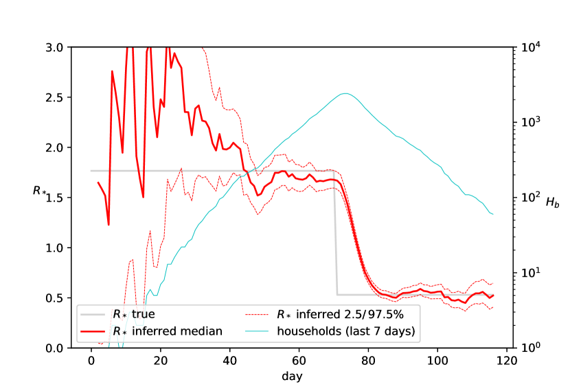
(b) with correction

Figure 8: Inference of $R_{*}$ during a simulated outbreak between-household inference updated daily, using the most recent $7$ days of data; and the within-household parameters known exactly. Sub-figure (a) omits the correction due to growth or decay, by setting $K_{(k,m)}=1$ in place of (13). Sub-figure (b) uses the method discussed in the text. The dotted red lines show the $2.5$ and $97.5$ percentiles of the posterior; the true value of $R_{*}$ is shown in grey; and the number of households infected in the most recent 7 days ($H_{b}$) is shown in light blue.

References

- [1] Root finding functions for Julia. https://github.com/JuliaMath/Roots.jl.
- Australian Government Department of Health [2014] Australian Government Department of Health. Australian Health Management Plan for Pandemic Influenza, April 2014.
- Ball and Neal [2002] F. G. Ball and P. Neal. A general model for stochastic SIR epidemics with two levels of mixing. Mathematical Biosciences, 180(1-2):73–102, 2002. doi: 10.1016/S0025-5564(02)00125-6.
- Ball et al. [1997] F. G. Ball, D. Mollison, and G. Scalia-Tomba. Epidemics with two levels of mixing. The Annals of Applied Probability, 7(1):46–89, 1997. doi: 10.1214/aoap/1034625252.
- Bezanson et al. [2017] J. Bezanson, A. Edelman, S. Karpinski, and V. B. Shah. Julia: A fresh approach to numerical computing. SIAM Review, 59(1):65–98, 2017. doi: 10.1137/141000671.
- Black [2019] A. J. Black. Importance sampling for partially observed temporal epidemic models. Statistics and Computing, 29:61–630, 2019. doi: 10.1007/s11222-018-9827-1.
- Black et al. [2013] A. J. Black, T. House, M. J. Keeling, and J. V. Ross. Epidemiological consequences of household-based antiviral prophylaxis for pandemic influenza. Journal of the Royal Society Interface, 10:20121019, 2013. doi: 10.1098/rsif.2012.1019.
- Black et al. [2017] A. J. Black, N. Geard, J. M. McCaw, J. McVernon, and J. V. Ross. Characterising pandemic severity and transmissibility from data collected during first few hundred studies. Epidemics, 19:61–73, 2017. doi: 10.1016/j.epidem.2017.01.004.
- Britton and Tomba [2019] T. Britton and G. Scalia Tomba. Estimation in emerging epidemics: biases and remedies. Journal of the Royal Society Interface, 16:20180670, 2019. doi: 10.1098/rsif.2018.0670.
- Champredon and Dushoff [2015] D. Champredon and J. Dushoff. Intrinsic and realized generation intervals in infectious-disease transmission. Proceedings of the Royal Society B, 282, 2015. doi: 10.1098/rspb.2015.2026.
- Cori et al. [2013] A. Cori, N. M. Ferguson, C. Fraser, and S. Cauchemez. A new framework and software to estimate time-varying reproduction numbers during epidemics. American Journal of Epidemiology, 178(9), 2013. doi: 10.1093/aje/kwt133.
- et al [2020] K. M. Gostic et al. Practical considerations for measuring the effective reproductive number, . medRxiv, 2020. doi: 10.1101/2020.06.18.20134858.
- for Disease Control and [CDC] Centres for Disease Control and Prevention (CDC). Principles of Epidemiology in Health Practice, Third Edition. U.S. Department of Health and Human Services, 2012. https://www.cdc.gov/csels/dsepd/ss1978/lesson1/section9.html.
- Geard et al. [2013] N. Geard, J. M. McCaw, A. Dorin, K. B. Korb, and J. McVernon. Synthetic population dynamics: a model of household demography. J. Artif. Soc. Simul., 16:8, 2013. doi: 10.18564/jasss.2098.
- Goldstein et al. [2009] E. Goldstein, K. Paur, C. Fraser, E. Kenah, J. Wallinga, and M. Lipsitch. Reproductive numbers, epidemic spread and control in a community of households. Mathematical Biosciences, 221(1):11–25, 2009. doi: 10.1016/j.mbs.2009.06.002.
- Health Protection Agency England [2009] Health Protection Agency England. “First Few Hundred” project, epidemiological protocols for comprehensive assessment of early swine influenza cases in the United Kingdom. 2009.
- Hilton and M. J [2019] J. Hilton and Keeling M. J. Incorporating household structure and demography into models of endemic disease. J. R. Soc Interface, 16:20190317, 2019. doi: 10.1098/rsif.2019.0317.
- House and M. J [2008] T. House and Keeling M. J. Deterministic epidemic models with explicit household structure. Mathematical Biosciences, 213:29–39, 2008. doi: 10.1016/j.mbs.2008.01.011.
- Hunter [2007] J. D. Hunter. Matplotlib: A 2D graphics environment. Computing In Science & Engineering, 9(3):90–95, 2007. doi: 10.1109/MCSE.2007.55.
- .id Consulting Pty. Ltd. [2020] .id Consulting Pty. Ltd. Australia: Household size (2016 census), January 2020. URL https://profile.id.com.au/australia/household-size.
- J et al. [2020] Griffin J, Casey M, Á Collins, K. Hunt, D. McEvoy, A. Byrne, C. McAloon, A. Barber, E. A. Lane, and S. More. Rapid review of available evidence on the serial interval and generation time of COVID-19. BMJ Open, 2020. doi: 10.1136/bmjopen-2020-040263.
- Koczkodaj et al. [2020] W. W. Koczkodaj, M. A. Mansournia, W. Pedrycz, A. Wolny-Dominiak, P. F. Zabrodskii, D. Strzałka, T. Armstrong, A. H. Zolfaghari, M. Dȩbski, and J. Mazurek. 1,000,000 cases of COVID-19 outside of China: the date predicted by a simple heuristic. Global Epidemiology, 2:100023, 2020. doi: 10.1016/j.gloepi.2020.100023.
- Link and Eaton [2012] W. A. Link and M. J. Eaton. On thinning of chains in MCMC. Methods in Ecology and Evolution, 2012. doi: 10.1111/j.2041-210X.2011.00131.x.
- Liu et al. [2018] Quan-Hui Liu, M. Ajelli, A. Aleta, S. Merler, Y. Moreno, and A. Vespignani. Measurability of the epidemic reproduction number in data-driven contact networks. PNAS, 115(50):12680–12685, 2018. doi: 10.1073/pnas.1811115115.
- McCaw et al. [2013] J. M. McCaw, K. Glass, G. Mercer, and J. McVernon. Pandemic controllability: a concept to guide a proportionate and flexible operational response to future influenza pandemics. Journal of Public Health, 36:5–12, 2013. doi: 10.1093/pubmed/fdt058.
- McLean et al. [2010] E. McLean et al. Pandemic (H1N1) 2009 influenza in the UK: clinical and epidemiological findings from the first few hundred (FF100) cases. Epidemiol. Infect., 138:1531–41, 2010. doi: 10.1017/S0950268810001366.
- Mercer et al. [2011] G. N. Mercer, K. Glass, and N. G. Becker. Effective reproduction numbers are commonly overestimated early in a disease outbreak. Statistics in Medicine, 30:984–994, 2011. doi: 10.1002/sim.4174.
- Mitchell and Ross [2016] L. Mitchell and J. V. Ross. A data-driven model for influenza transmission incorporating media effects. Royal Society Open Science, 3, 2016. doi: 10.1098/rsos.160481.
- Mossong et al. [2008] J. Mossong, N. Hens, M. Jit, P. Beutels, K. Auranen, R. Mikolajczyk, et al. Social contacts and mixing patterns relevant to the spread of infectious diseases. PLoS Med., 5:e74, 2008. doi: 10.1371/journal.pmed.0050074.
- Pellis et al. [2012] L. Pellis, F. Ball, and P. Trapman. Reproduction numbers for epidemic models with households and other social structures I: Definition and calculation of R0. Math. Biosci., 235:85–97, 2012. doi: 10.1016/j.mbs.2011.10.009.
- Pollett [2003] P. K. Pollett. Integrals for continuous-time Markov chains. Mathematical Biosciences, 182:213–225, 2003. doi: 10.1016/s0025-5564(02)00161-x.
- Pollett and Stefanov [2002] P. K. Pollett and V Stefanov. Path integrals for continuous-time Markov chains. Journal of Applied Probability, 39:901–904, 2002. doi: 10.1239/jap/1037816029.
- Price et al. [2020] D. J. Price, F. M. Shearer, M. T. Meehan, E. McBryde, R. Moss, N. Golding, P. Dawson, D. Cromer, J. Wood, S. Abbott, J. McVernon, and J. M. McCaw. Early analysis of the Australian COVID-19 epidemic. eLife, 9:e58785, 2020. doi: 10.7554/eLife.58785.
- Rebuli et al. [2018] N. P. Rebuli, N. G. Bean, and J. V. Ross. Estimating the basic reproductive number during the early stages of an emerging epidemic. Theoretical Population Biology, 119:26–36, 2018. doi: 10.1016/j.tpb.2017.10.004.
- Reed et al. [2013] C. Reed, M. Biggerstaff, L. Finelli, L. M. Koonin, D. Beauvais, A. Uzicanin, et al. Novel framework for assessing epidemiologic effect of influenza epidemics and pandemics. Emerg. Infect. Dis., 19:85–91, 2013.
- Riley et al. [2015] P. Riley, M. Ben-Nun, J. A. Linker, A. A. Cost, J. L. Sanchez, D. George, D. P. Bacon, and S. Riley. Early characterization of the severity and transmissibility of pandemic influenza using clinical episode data from multiple populations. PLoS Comp. Biol., 11:e1004392, 2015. doi: 10.1371/journal.pcbi.1004392.
- Ross et al. [2010] J. V. Ross, T. House, and M. J. Keeling. Calculation of disease dynamics in a population of households. PLoS ONE, 5(3):e9666, 2010. doi: 10.1371/journal.pone.0009666.
- Schön et al. [2018] T. B. Schön, Å. Svensson, L. Murray, and F. Lindsten. Probabilistic learning of nonlinear dynamical systems using sequential Monte Carlo. Mechanical Systems and Signal Processing 104, 104:866–883, 2018. doi: 10.1016/j.ymssp.2017.10.033.
- Thompson et al. [2019] R. N. Thompson, J. E. Stockwind, R. D. van Gaalen, J. A. Polonsky, Z. N. Kamvar, P. A. Demarsh, E. Dahlqwist, S. Li, E. Miguel, T. Jombart, J. Lessler, S. Cauchemez, and A. Cori. Improved inference of time-varying reproduction numbers during infectious disease outbreaks. Epidemics, 29:100356, 2019. doi: 10.1016/j.epidem.2019.100356.
- Tomba et al. [2010] G. Scalia Tomba, Å. Svensson, T. Asikainen, and J. Giesecke. Some model based considerations on observing generation times for communicable diseases. Mathematical Biosciences, 223(1):24–31, 2010. doi: 10.1016/j.mbs.2009.10.004.
- van Gageldonk-Lafeber et al. [2012] A. B. van Gageldonk-Lafeber, van der Sande M. A., A. Meijer, I. H. Friesema, G. A. Donker, J. Reimerink, et al. Utility of the first few100 approach during the 2009 influenza A(H1N1) pandemic in the Netherlands. Antimicrob. Resist. Infect. Control, 1:30, 2012. doi: 10.1186/2047-2994-1-30.
- Walker et al. [2017] J. N. Walker, J. V. Ross, and A. J. Black. Inference of epidemiological parameters from household stratified data. PLoS ONE, 12:e0185910, 2017. doi: 10.1371/journal.pone.0185910.
- Walker et al. [2019] James N. Walker, Andrew J. Black, and Joshua V. Ross. Bayesian model discrimination for partially-observed epidemic models. Mathematical Biosciences, 317:108266, Nov 2019. doi: 10.1016/j.mbs.2019.108266.
- World Health Organization [2017] World Health Organization. WHO guidance for surveillance during an influenza pandemic, 2017.
- World Health Organization [2021] World Health Organization. Weekly epidemiological update on COVID-19 - 4 May 2021, 4 May 2021. URL https://www.who.int/publications/m/item/weekly-epidemiological-update-on-covid-19---4-may-2021.