$\mathsf{DeepQR}$: Neural-based Quality Ratings for Learnersourced Multiple-Choice Questions

Abstract

Automated question quality rating (AQQR) aims to evaluate question quality through computational means, thereby addressing emerging challenges in online learnersourced question repositories. Existing methods for AQQR rely solely on explicitly-defined criteria such as readability and word count, while not fully utilising the power of state-of-the-art deep-learning techniques. We propose $\mathsf{DeepQR}$, a novel neural-network model for AQQR that is trained using multiple-choice-question (MCQ) datasets collected from PeerWise, a widely-used learnersourcing platform. Along with designing $\mathsf{DeepQR}$, we investigate models based on explicitly-defined features, or semantic features, or both. We also introduce a self-attention mechanism to capture semantic correlations between MCQ components, and a contrastive-learning approach to acquire question representations using quality ratings. Extensive experiments on datasets collected from eight university-level courses illustrate that $\mathsf{DeepQR}$ has superior performance over six comparative models.

1 Introduction

Recent shifts towards online learning at scale have presented new challenges to educators, including the need to develop large repositories of content suitable for personalised learning and to find novel ways of deeply engaging students with such material (Dhawan 2020; Davis et al. 2018). Learnersourcing has recently emerged as a promising technique for addressing both of these challenges (Kim 2015). Akin to crowdsourcing, learnersourcing involves students in the generation of educational resources. In theory, students benefit from the deep engagement needed to generate relevant learning artefacts which leads to improved understanding and robust recall of information, a phenomenon known as the generation effect (Crutcher and Healy 1989). In addition, the large quantity of resources created from learnersourced activities can be used by students to support regular practice, which is known to be a highly effective learning strategy (Roediger III and Karpicke 2006; Carrier and Pashler 1992), especially when spaced over time and when feedback is provided (Kang 2016).

Despite the well-established benefits of learnersourcing for students (Moseley, Bonner, and Ibey 2016; Ebersbach, Feierabend, and Nazari 2020), evaluating and maintaining the quality of student-generated repositories is a significant challenge (Walsh et al. 2018; Moore, Nguyen, and Stamper 2021). Low quality content can dilute the value of a learnersourced repository, and negatively affect students’ perceptions of its usefulness. On the other hand, the identification of high-quality content can facilitate useful recommendations to students when practicing. Therefore, approaches for accurately assessing the quality of student-generated resources are of great interest. Involving domain experts in the evaluation process is very costly and does not scale, negating one of the key benefits of learnersourcing. A more scalable solution is to have students review and evaluate the content themselves (Darvishi, Khosravi, and Sadiq 2021). Prior research has shown that students can make similar quality judgments to experts, especially when the assessments provided by multiple students are aggregated (Abdi et al. 2021). However, a sufficient number of students must view and evaluate each artefact before a valid assessment can be produced, which is inefficient. Computing quality assessments of content, at the moment it is produced, would benefit all learners. Such a priori assessment of quality remains a difficult yet important challenge in learnersourcing contexts.

Current learnersourcing tools support a wide variety of artefact types, including hints, subgoal-labels, programming problems and complex assignments (Mitros 2015; Kim, Miller, and Gajos 2013; Leinonen, Pirttinen, and Hellas 2020; Pirttinen et al. 2018; Denny et al. 2011). Multiple-choice questions (MCQs) are a very popular format in learnersourcing platforms, appearing in tools such as RiPPLE (Khosravi, Kitto, and Williams 2019), Quizzical (Riggs, Kang, and Rennie 2020), UpGrade (Wang et al. 2019) and PeerWise (Denny, Luxton-Reilly, and Hamer 2008). Hence, a generalisable model that can assess the quality of student-generated MCQs has the potential for a significant impact.

In this work, we explore the problem of automated question quality rating (AQQR) by developing a computational method to rate student-generated MCQs a priori. Existing measures of MCQ quality target explicitly-defined features such as cognitive complexity with respect to Bloom’s taxonomy (Bates et al. 2014), the justification of rationales (Choi, Land, and Turgeon 2005), and the feasibility of distractors (Papinczak et al. 2012; Galloway and Burns 2015). Such measures require costly and subjective manual evaluation by experts. Recent progress in natural language processing (NLP) provides a suite of tools for extracting and analysing rich features of texts, presenting a real opportunity to enhance existing measures of quality.

Contribution.

We propose $\mathsf{DeepQR}$, a novel neural network-based model for AQQR that is trained using datasets collected from student-generated MCQ repositories. $\mathsf{DeepQR}$ is designed to be used in learnersourcing platforms to provide useful and immediate feedback to students and instructors. Figure 1 illustrates a potential use of $\mathsf{DeepQR}$ in practice. To the best of our knowledge, this is the first work that employs deep learning techniques to produce ratings of question quality. The design of $\mathsf{DeepQR}$ is guided by three research goals: (1) Capitalise on existing work that has identified indicative criteria for question quality – such as readability or word count – and utilise these for AQQR using tools from NLP. In particular, we investigate the extraction of correlations between various MCQ components: the question stem, the correct answer, the distractors and explanation. (2) Given the immense success of neural-based models for natural language understanding, it is natural to consider their application to the extraction of meaning from MCQs. The second research goal thus seeks to utilise rich semantic features to solve AQQR. (3) The research goals above suggest two sources of input features that are potentially useful for AQQR, namely, the explicitly-defined features (EDF) discussed in (1), and the semantic features (SF) discussed in (2). The third research goal is to explore their “interplay”, i.e., how combining EDF with SF could facilitate a superior model for AQQR.

To answer (1), we propose two complementary models: the first is an AQQR model that takes 18 EDFs as input including word counts, clarity, correctness, and readability indices. Since these features were not designed to capture relations between different question components, in the second model, we employ a self-attention mechanism that discovers semantic-based correlations of question components (SCQC). We demonstrate that enriching the input features in the first model with SCQC drastically improves AQQR performance. To answer (2), we design a model that feeds GloVe embeddings into a transformer to produce a representation that captures the semantics of an MCQ. We demonstrate that this semantic feature-based model solves AQQR with better performance than benchmark models such as $\mathsf{RoBERTa}$ and $\mathsf{SBERT}$ which are much more costly to train, and at a comparable performance as the second model designed for (1). This demonstrates the value of semantic features (SF) in estimating question quality. To answer (3), we propose the $\mathsf{DeepQR}$ model by combining EDF, SCQC, and SF as discussed above. Furthermore, to improve performance, we introduce a quality-driven question embedding (QDQE) scheme, which employs contrastive learning to fine-tune GloVe embeddings and better reflect question quality. This embedding is then used to enhance our model, providing a considerable performance boost. Our experiments were conducted using eight datasets (comprising 15,350 questions and more than 1,000,000 student-assigned quality ratings) from the PeerWise (Denny, Luxton-Reilly, and Hamer 2008) learnersourcing platform, collected from medicine and commercial law courses. For most courses, our model is able to achieve accuracy in excess of 80% (see Section 5). We also conduct a systematic analysis to validate our design decisions and the applicability of our model.

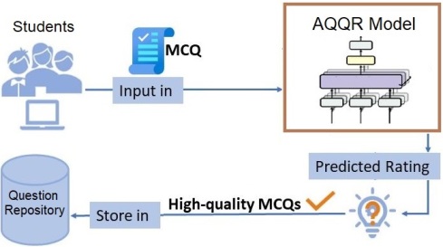
Figure 1: $\mathsf{DeepQR}$ used in a learnersourcing platform to remove low-quality student-generated questions.

2 Related Work

Evaluating the quality of questions has attracted significant interest in educational research. Standard metrics from classical test theory and item response theory, such as discrimination indices, have been used for decades to aid instructors in identifying poor quality questions (Brown et al. 2021; Malau-Aduli et al. 2014). However, computing such quantitative measures requires large quantities of data on student responses to items. Various qualitative indicators have also been proposed and used, such as question clarity (Choi, Land, and Turgeon 2005) and distractor-plausibility (Bates et al. 2014). Prior studies assessing such qualitative measures, however, have involved significant manual effort by experts. In learnersourcing contexts, aggregating student ratings to assess the quality of questions is scalable and agrees well with expert ratings of quality (Abdi et al. 2021; Darvishi, Khosravi, and Sadiq 2021; McQueen et al. 2014). In our own work, we use averaged student ratings as ground-truth labels when training our AQQR models.

AQQR has recently attracted the attention of the machine learning community. In particular, the inaugural NeurIPS 2020 Education Challenge included a quality prediction task for mathematics questions (Wang et al. 2020). Two of the successful entries in the NeurIPS challenge relied on explicitly-defined features (EDF), such as difficulty and readability, deriving a final rating using some form of average over these feature values (Shinahara and Takehara 2020; The Machine Learning Team, TAL Education Group, Beijing, China 2020). Such approaches are limited in the sense that they rely on ad-hoc EDFs and linear transformations which may not provide the level of robustness and flexibility required for a diverse range of questions and courses. Neural networks are able to extract distributional semantics from texts offering greater richness and versatility. Yet, to our knowledge, there has not been a systematic effort to design neural-based models to rate question quality. Our paper aims to fill this gap by investigating the value of semantic features (SF) in AQQR. We note that the question dataset published for the NeurIPS 2020 Education Challenge is not suitable for our purpose as the questions are largely mathematical and involve diagrams.

Tasks that closely resemble AQQR – and for which neural network-based approaches have proven useful – include question difficulty prediction (QDP) and automated essay scoring (AES). QDP requires evaluation of a difficulty score for reading comprehension questions. Huang et al. (2017) approached this task using deep learning with an attention-based CNN model, and subsequent work by Qiu, Wu, and Fan (2019) incorporated a knowledge extraction aspect. Both works rely heavily on the extraction of rich SFs from a question to predict its difficulty. AES seeks to rate an article’s quality based on its content, grammar, and organization. Early AES models generally applied regression methods to a set of EDFs (Shermis and Burstein 2003). Taghipour and Ng (2016) was the first to tackle AES using deep learning by automating feature extraction using a combination of convolutional and recurrent neural networks. More recently, Uto, Xie, and Ueno (2020) combined EDF input and SF extracted from the pre-trained language model Bidirectional Encoder Representations from Transformers ($\mathsf{BERT}$).

Pre-trained language models have brought major breakthroughs with significant performance improvement and training cost savings in NLP (Bommasani et al. 2021). Relying on its powerful language representation ability and easy scalability for various downstream tasks, $\mathsf{BERT}$(Devlin et al. 2019) and its extended models often appear at the forefront of the NLP benchmark leaderboards. Among them, $\mathsf{RoBERTa}$ (Liu et al. 2019) improves $\mathsf{BERT}$ by pre-training on a larger dataset with more parameters; while Sentence-BERT($\mathsf{SBERT}$) (Reimers and Gurevych 2019) is trained using siamese $\mathsf{BERT}$-Networks on paired sentences to derive better semantic embeddings. Both of them outperform $\mathsf{BERT}$ in well-established benchmark tasks.

3 Problem Formulation

Here we formally define the automated question quality rating (AQQR) task. Each PeerWise dataset that specifies an instance of the task contains student-authored questions for a university course. When authoring an MCQ, the student specifies seven components: a question stem, a correct answer, (up to) four distractors, and a paragraph that explains the idea and rationale behind the question. The question is then submitted to an online question repository accessible by the class. After answering a question, a student may leave a holistic quality rating (from $0,1,\ldots,5$) by considering the “language, quality of options, quality of explanation, and relevance to the course” as suggested by the system. We provide a sample MCQ below:

• Stem: Mr. Cram-zan is chilling in his room wondering another new way in which to make money. He believes he should create a global footballing league as God is telling him to. He is the chosen one, not Mourinho. He also thinks his close friend, Moo Leerihan, is plotting the downfall of his league. What is Mr. Cram-zan suffering from? • Answer: Schizophrenia • Distractor 1: Hallucinations    Distractor 2: Illusions • Distractor 3: Over ambition    Distractor 4: Being too chilled • Explanation: Schizophrenia would be the SBA as it encompasses all the aspects. • Average rating: 2.71

Definition 1

(AQQR) Given a set of MCQ $M_{1},M_{2},\ldots,M_{n}$ collected from a course, where each $M_{i}$ consists of a stem $S_{i}$, a correct answer $A_{i}$, distractors $D_{i,j}$ where $j\in\{1,2,3,4\}$, explanation $E_{i}$, and is assigned a rating $r_{i}$, AQQR seeks to build a prediction model $\mathsf{Rate}$ that estimates the rating of MCQ in the newly-conducted test set.

We view AQQR as consisting of two subtasks: (1) MCQ representation aims to process the input data to form feature vectors. The features are manually specified or automatically extracted. The former extracts explicitly-defined features (EDF) by leveraging domain knowledge and expert judgement while the latter captures semantic features (SF) using machine learning algorithms. We speculate that both types of features could be useful for our task. (2) MCQ modelling aims to construct a prediction model for the quality rating given the feature vectors. In this paper, we adopt a simple linear layer for MCQ modelling. Thus the main focus of our method is on MCQ representation. See Figure 2 for an overview of these two subtasks.

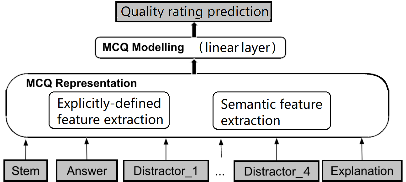
Figure 2: An overview of AQQR subtasks.

4 Methods

In this section, we first describe how EDF are extracted and used in AQQR. This is then followed by a description of our transformer-based SF extraction method. Last, we present our $\mathsf{DeepQR}$ model which combines modules developed for both preceding parts. Overall this section will present 5 AQQR models. Fig. 3 presents an architectural overview.

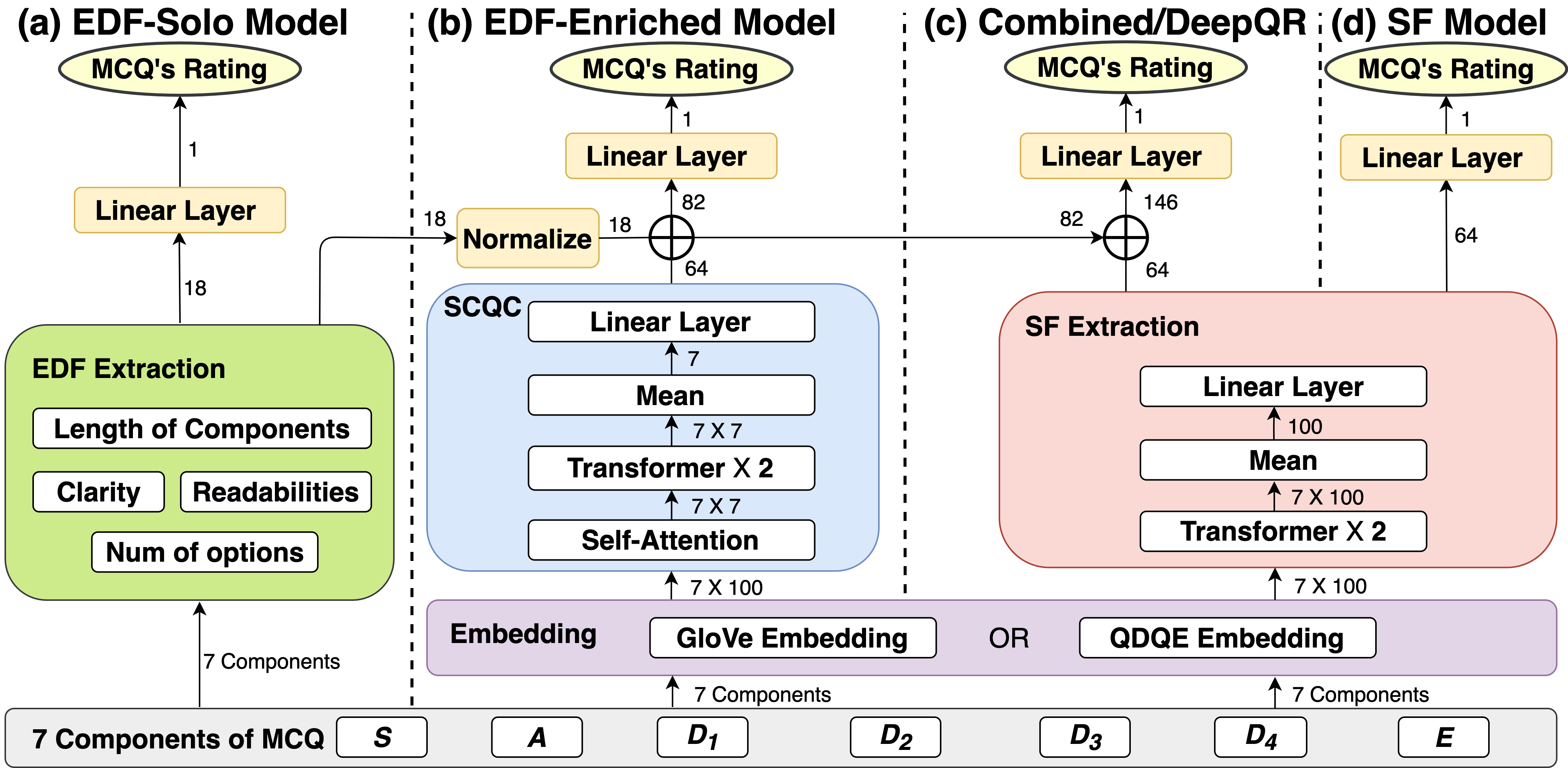
Figure 3: The overall architecture of the introduced AQQR models.

4.1 EDF-based Models

Earlier pedagogical research have identified EDF which determine the quality of MCQ (Papinczak et al. 2012; Bates et al. 2014; Galloway and Burns 2015). We introduce two EDF-based AQQR models: $\mathsf{EDF\mathchar 45\relax Solo}$ and $\mathsf{EDF\mathchar 45\relax Enriched}$. The former trains linear weights of 18 EDF computed directly from the input texts. This model echoes earlier methods, e.g., winning bids of NeurIPS 2020 Education Challenge. The latter enriches the input of $\mathsf{EDF\mathchar 45\relax Solo}$ using semantic correlations between MCQ components (SCQC), extracted by a self-attention mechanism.

Explicity-defined features. Details of the selected EDF are in Table 1. The grammatical error $\gamma_{i}$ is obtained using LanguageTool (Naber 2003). The nine readability indices (DuBay 2004) characterise suitable reader groups of a text (e.g., by revealing the cognitive complexity required to make sense of the text) in different ways. A common feature of these indices is the use of key parameters such as average word count per sentence and number of syllables per word.

The $\mathsf{EDF\mathchar 45\relax Solo}$ model. To measure the quality of a question, classical models generally use manually-defined linear transformations on a set of EDF. In the $\mathsf{EDF\mathchar 45\relax Solo}$ model, we also use a linear transformation (of the 18 selected EDF) but the weights for the features are trained using linear regression with MSE (mean square error) loss. See Fig. 3(a): For MCQ $M_{i}$, the predicted quality rating is

$$\begin{aligned} \leavevmode\resizebox{91.05649pt}{}{$\hat{r}_{i}=\begin{array}[]{ccc}\overrightarrow{w_{\mathrm{lin}}}\cdot\overrightarrow{\mathrm{EDF}}_{i}+b_{\mathrm{lin}}\end{array}$}\end{aligned}$$ (1)

where $\overrightarrow{\mathrm{EDF}}=[n_{\mathrm{op}},\nu_{S},\ldots,\nu_{E},\gamma,\mathrm{rd}_{1},\ldots,\mathrm{rd}_{9}]$, $\overrightarrow{w_{\mathrm{lin}}}$ & $b_{\mathrm{lin}}$ are (18-dim) trainable weights & bias, resp.

Table 1: Explicitly defined features.

Feature Type	Features
Options	Number of options $n_{\mathrm{op},i}$
Length	word counts $\nu_{C}$, where $C$ is taken from $\{S_{i},A_{i},D_{i,1},\ldots,D_{i,4},E_{i}\}$
Correctness	Grammatical error rate $\gamma_{i}$
Readability	Flesch reading ease $\mathrm{rd}_{i,1}$; Flesch–Kincaid $\mathrm{rd}_{i,2}$; fog $\mathrm{rd}_{i,3}$; Coleman–Liau $\mathrm{rd}_{i,4}$; Linsear write formula $\mathrm{rd}_{i,5}$; Automated readability index $\mathrm{rd}_{i,6}$; Spache $\mathrm{rd}_{i,7}$; Dale–Chall $\mathrm{rd}_{i,8}$; SMOG $\mathrm{rd}_{i,9}$ (DuBay 2004)

Semantic correlation of MCQ components. The quality of distractors of an MCQ should be assessed in the context of other components. Indeed, a “good” distractor is expected to bear certain syntactic or semantic correlations with the question stem, correct answer, and possibly other distractors. We thus design SCQC to capture these correlations; See Figure 3 (b). The input to SCQC consists of semantic embeddings of all component: $\overrightarrow{\mathrm{Re}}=\left[\mathrm{Re}_{S},\mathrm{Re}_{A},\ldots,\mathrm{Re}_{E}\right]$, where each $\mathrm{Re}_{C}\in\mathbb{R}^{d_{\mathrm{em}}}$ is a $d_{\mathrm{em}}$-dim embedding of component $C\in\{S,\ldots,E\}$. These embeddings are assumed to be produced by a separate algorithm (See below). SCQC utilises a self-attention mechanism to interpret correlations:

$$\begin{aligned} \mathrm{Co}&=\mathrm{A{\scriptstyle TTENTION}}\left(\overrightarrow{\mathrm{Re}},\overrightarrow{\mathrm{Re}}\right),\\ \mathrm{A{\scriptstyle TTENTION}}(V,Q)&=\mathrm{softmax}\left(V^{\mathrm{T}}WQ\right),\end{aligned}$$ (2)

where $Q$ is a query sequence on the context sequence $V$, $W\in\mathbb{R}^{d_{\mathrm{em}}\times d_{\mathrm{em}}}$ trainable weight matrix, and the attention score matrix $\mathrm{Co}\in\mathbb{R}^{7\times 7}$ represents component-wise correlations. We then encode this matrix by a 2-layer transformer encoder. Each transformer layer contains two sub-layers: a self-attention mechanism and a feed-forward layer, each of which has a residual connection before normalisation (Vaswani et al. 2017). Thus the output of each sub-layer is $\mathrm{LayerNorm}(X+\mathrm{Sublayer}(X))$ where $X$ is input, $\mathrm{LayerNorm}$ is the normalisation function, and $\mathrm{Sublayer}$ is either self-attention or feed-forward as described in (3) and (4), respectively. Set the query, key, and value matrices as $Q=XW^{Q},K=XW^{K},V=XW^{V}$ where $W^{Q},W^{K},W^{V}$ are $d_{\mathrm{tr}}\times d_{\mathrm{tr}}$ trainable matrices, respectively.

$$\begin{aligned} \leavevmode\resizebox{202.3529pt}{}{$\mathrm{S{\scriptstyle ELF}A{\scriptstyle TTENTION}}(Q,K,V)=\mathrm{softmax}\left(\frac{QK^{\mathrm{T}}}{\sqrt{d_{\mathrm{tr}}}}\right)V$}\end{aligned}$$ (3)

$$\begin{aligned} \leavevmode\resizebox{212.47287pt}{}{$\mathrm{F{\scriptstyle EED}F{\scriptstyle ORWARD}}(X)=\max\left(0,XW_{1}+\vec{b_{1}}\right)W_{2}+\vec{b_{2}}$}\end{aligned}$$ (4)

where $W_{1},W_{2}$ are trainable weights and $\vec{b_{1}}$ and $\vec{b_{2}}$ are biases. The input to the first transformer layer is the correlation matrix $\mathrm{Co}$ and the next layer’s input is the output of the previous layer. The output of the 2-layer transformer is a $7\times 7$ matrix representing the encoded correlations. Finally, we compute the average attention score for each component which is fed into a linear layer to produce the SCQC output. Note that the parameters of SCQC are trained using prediction loss and thus SCQC captures in some sense the impact of each component to the question quality. We will showcase the ability of SCQC using a case study in Section 5.3.

The $\mathsf{EDF\mathchar 45\relax Enriched}$ model. See Figure 3(b). The model concatenates the normalized EDF with SCQC output before applying a linear layer (similar to (1)) to obtain the rating prediction. We fix the popular GloVe word embeddings (Pennington, Socher, and Manning 2014) to represent the MCQ components as inputs to the SCQC module. GloVe was trained with local as well as global statistics of a corpus and is able to capture semantic similarity using much lower dimensional vectors than other popular word embeddings.

4.2 SF-based Model

Given the success of neural networks in building rich representations in multiple NLP tasks, it is reasonable to expect that deep semantic information captured by such models may also serve the purpose of AQQR. This section presents our method to extract such semantic information. Just as for SCQC, we use a 2-layer transformer encoder. The input of the encoder is word embeddings of the MCQ components. The transformer consists of two multi-head self-attention layers (Vaswani et al. 2017):

$$\begin{aligned} \mathrm{M{\scriptstyle ULTI}H{\scriptstyle EAD}}(Q,K,V)=\left(\bigoplus_{j=1}^{h}\mathrm{head}_{j}\right)W^{O}\\ \mathrm{head}_{j}=\mathrm{S{\scriptstyle ELF}A{\scriptstyle TTENTION}}\left(QW^{Q}_{j},KW^{K}_{j},VW^{V}_{j}\right).\end{aligned}$$ (5)

Here, $\oplus$ is concatenation, $W^{Q}_{j},W^{K}_{j},W^{V}_{j}\in\mathbb{R}^{d_{\mathrm{tr}}\times(d_{\mathrm{tr}}/h)}$, $W^{O}\in\mathbb{R}^{d_{\mathrm{tr}}\times{d_{\mathrm{tr}}}}$, and $h$ the head count (set $h=4$). Having multiple heads allows the discovery of richer information as different heads may focus on different aspects of the data. We then average the obtained representation and apply a linear transformation to get the final SF representation.

Figure 3(d) summarises the architecture of the $\mathsf{SF}$ model. We again adopt GloVe as input embedding to the SF extraction module. After obtaining the SF representation, the $\mathsf{SF}$ model applies a final linear layer (similarly to (1)) to obtain the predicted quality rating. We mention that efficiency amounts to a key advantage of our method. Indeed, it is straightforward to train (heavyweight) models such as $\mathsf{RoBERTa}$ and $\mathsf{SBERT}$ from the input corpus. Yet, we will demonstrate in Sec.5.2 that this does not improve performance while incurring heavier training costs.

4.3 Models Combining EDF and SF

This section presents two models that combine the EDF and SF in the hope to make the best use of the extracted features.

The $\mathsf{Combined}$ model.

Following Figure 3(c), the model takes the normalised EDF concatenated with SCQC, which is then concatenated with the extracted SF above. The combined vector is applied a linear transformation as in the models above to produce a quality rating prediction. The model parameters of SCQC and the SF extraction module are trained using the prediction loss. The input embedding to both SCQC and the SF extraction modules are GloVe, which is obtained without quality consideration. This inspires us to fine-tune GloVe to strengthen the representations of MCQ.

Quality-driven question embedding and $\mathsf{DeepQR}$ model.

The $\mathsf{DeepQR}$ model differs from $\mathsf{Combined}$ in that it adopts QDQE for its input instead of GloVe embeddings. QDQE builds question representations while taking into account their quality rating. For this, we adopt a (supervised) contrastive learning algorithm to fine-tune a baseline language model. Contrastive learning gained considerable interest recently as a generic representation learning framework (Chen et al. 2020; Giorgi et al. 2021). Supervised contrastive learning leverages label information in a dataset (Gunel et al. 2021). In a nutshell, QDQE fine-tunes question embeddings derived from GloVe with a one-layer transformer encoder, so as to push apart representations of MCQ with “unmatched quality ratings”, while pulling together representations of MCQ with “matching quality ratings”.

More specifically, we build a dataset $\mathcal{D}_{\mathrm{CL}}$ consisting of triples of questions. Assume our training set contains MCQ $M_{1},\ldots,M_{n}$, sorted in ascending order of quality rating. Set $S_{L}=\{M_{1},\ldots,M_{c}\}$ and $S_{H}=\{M_{n-c+1},\ldots,M_{n}\}$ where $c<n/2$ is a fixed integer. The dataset set $\mathcal{D}_{\mathrm{CL}}$ contains triples of the form $(a,pos,neg)$: For each $(a,pos)\in S^{2}_{H}$ ($S^{2}_{L}$), choose a random $n_{a,pos}\in S_{L}$ ($S_{H}$). Then $\mathcal{D}_{\mathrm{CL}}=\{(a,pos,neg)\mid(a,pos)\in S^{2}_{L}\cup S^{2}_{H},neg=n_{a,pos}\}$. Note that there are in total $2c(c-1)$ triples.

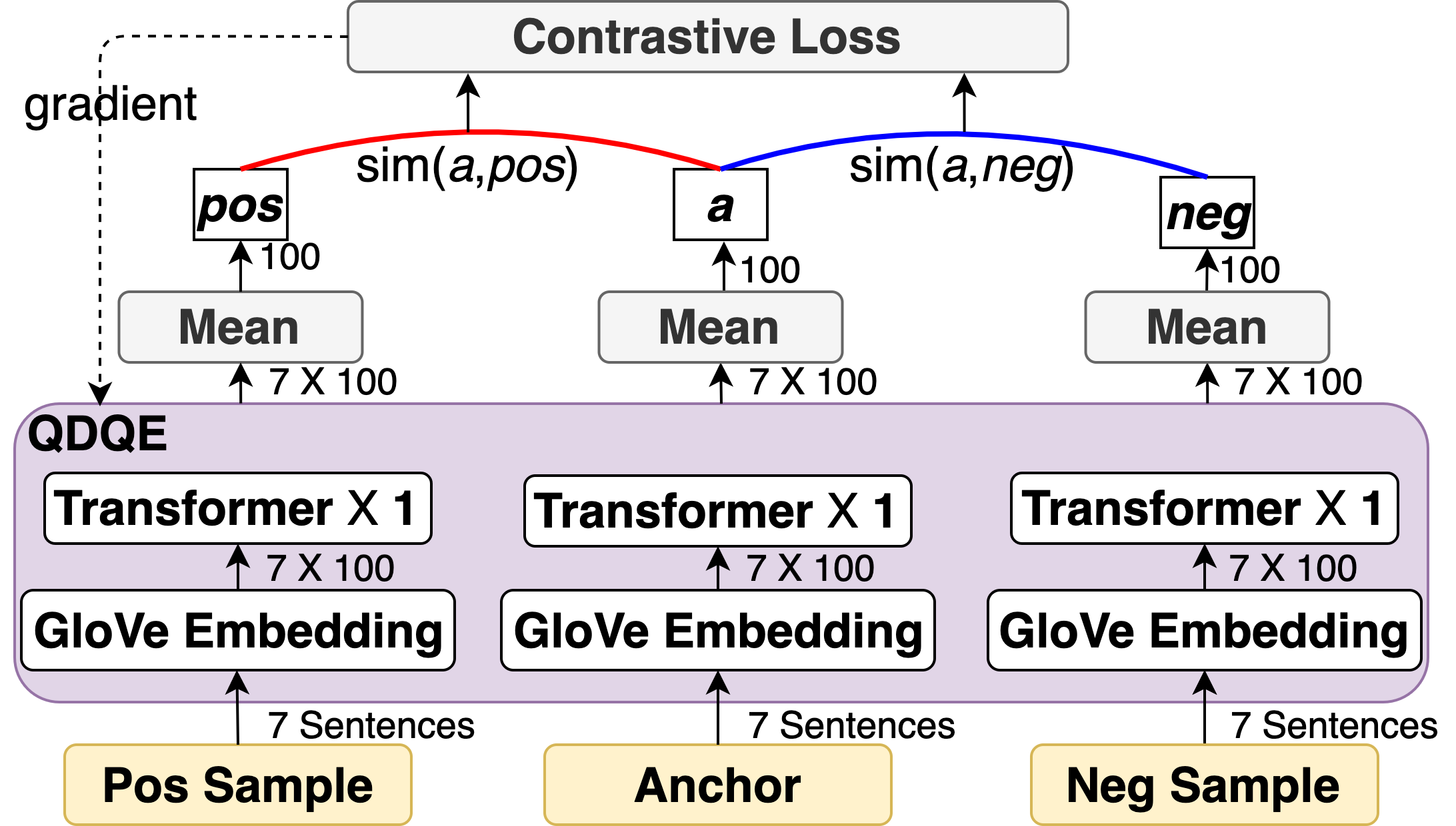
Figure 4: The QDQE algorithm builds MCQ representations using (supervised) contrastive learning.

Figure 4 shows the model for training QDQE. The model starts from $d$-dim GloVe embeddings of the MCQ components for questions in a $(a,pos,neg)$ triple. These embeddings are encoded by a transformer that produces for each question a $7\times d$ encoded matrix. A $d$-dim vector is then computed by taking the mean of each column of the encoded matrix for each question in the triple. The contrastive loss is the InfoNCE function $\mathcal{L}_{\mathrm{IN}}$ (Oord, Li, and Vinyals 2018):

where $sim$ used here is cosine similarity, and $\tau=0.07$ following MoCo (He et al. 2020). In this way, we hope the distance between the QDQE vectors $\vec{a}$ and $\vec{p}$ becomes less than the distances between $\vec{a}$ and $\vec{n}$, as well as between $\vec{p}$ and $\vec{n}$.

5 Experiments

5.1 Experiment Setup

Datasets. Our eight PeerWise datasets are taken from a law course and seven medicine courses (M1,4,7 are the same course of a university in different school years, similar for M2,3,5,6). Each dataset contains MCQ that are presented as in Section 3 where the average rating is the ground truth. To ensure the reliability, only questions receive at least 10 ratings are included. See Table 2 for the final datasets details.

Table 2: The details of the eight PeerWise datasets.

Subject	Law	M1	M2	M3
# MCQ	3,834	1,747	1,509	2,021
# ratings	72,753	141,889	92,607	152,387
Ratings per MCQ	18.97	81.21	61.36	75.40
Av. stem length	101.75	198.29	112.21	130.93
Subject	M4	M5	M6	M7
# MCQ	1,205	2,879	1,250	905
# ratings	143,654	219,084	91,719	109,549
Ratings per MCQ	119.21	76.09	73.37	121.04
Av. stem length	246.96	163.40	192.45	190.25

Models. We test five AQQR models ($\mathsf{EDF\mathchar 45\relax Solo}$, $\mathsf{EDF\mathchar 45\relax Enriched}$, $\mathsf{SF}$, $\mathsf{Combined}$, $\mathsf{DeepQR}$) and two benchmark models $\mathsf{RoBERTa}$ and $\mathsf{SBERT}$. The benchmark models are implemented using roberta-base and sentence-transformers/paraphrase-distilroberta-base-v1 from Huggingface (Wolf et al. 2019), resp. and are fine-tuned on AQQR. For these benchmarks we combine all MCQ components as a single input. We split each dataset into training, validation, test set by 8:1:1. We use a seed of 2021, and train our models using Adam optimizer (Kingma and Ba 2015) for 50 epochs from which the epoch achieves the lowest validation loss (MSE: mean square error) is chosen.

Performance measures. We use both MSE and ACC to measure AQQR performance. For ACC, we count a predicted rating as correct when $|r_{i}-\hat{r}_{i}|\leq 0.25$ (recall $r_{i}$ & $\hat{r}_{i}$ are resp. the ground truth & predicted labels) and define ACC as the fraction of correct predictions in the test set. While ACC offers insight on the model’s ability, MSE can be seen as a more reliable metric.

Hyper-parameters. We set the batch size to 16 and the initial learning rate to $1e-3$. For the optimizer learning rate scheduler, we set step size to 3 and gamma to 0.7 for the optimizer learning rate scheduler. We set the dropout to 0.5 for our AQQR models and to 0.1 for the two benchmarks. For QDQE, we train a model separately for each course dataset with c = 80 and 20 for the train and validation dataset respectively. The hyper-parameter settings are inherited from benchmark models except the batch size is 1.

Experiments design. We conduct experiments in three stages to verify modules within our design. We first compare $\mathsf{EDF\mathchar 45\relax Solo}$ with $\mathsf{EDF\mathchar 45\relax Enriched}$ to highlight the power of $\mathsf{SCQC}$, and then compare $\mathsf{SF}$ with $\mathsf{RoBERTa}$ and $\mathsf{SBERT}$ to showcase our SF extraction module. We last demonstrate the value of the combined models $\mathsf{Combined}$ and $\mathsf{DeepQR}$ hoping to validate the use of QDQE.

5.2 Results

All experiments are conducted on NVIDIA 460.84 Linux Driver. The CUDA version is 11.2 and the Quadro RTX 8000 with 48 GB GPU memory for our experiment. The CPU version is Intel(R) Xeon(R) Gold 5218 CPU @ 2.30GHz and 16 cores. The results are shown in Table 3. We make the following observations: (1) As seen from the first two rows, $\mathsf{EDF\mathchar 45\relax Enriched}$ made a substantial improvement from $\mathsf{EDF\mathchar 45\relax Solo}$ across all datasets, achieving almost $80\%$ less MSE for M7 and $43\%$ less MSE for M6 less. This reflects the result after enriching the EDF with SCQC. (2) Among the SF-based models, $\mathsf{SF}$ outperforms the benchmarks of $\mathsf{RoBERTa}$ and $\mathsf{SBERT}$ in most of the cases, and performs comparably well as $\mathsf{EDF\mathchar 45\relax Enriched}$. This demonstrates that deep learning captures sufficient semantic information to express question quality. (3) In general, the models that combine EDF and SF achieve the best accuracy. This is despite the fact that $\mathsf{Combined}$’s lead is not conclusive on some of the datasets, e.g., getting higher loss than other models in Law and M1. This is somewhat surprising as enlarging the input features does not necessarily boost the performance. Nevertheless, $\mathsf{DeepQR}$ scores the best performance across all datasets in terms of both MSE and ACC. The only two exceptions are the ACC scores on Law and M5 which are within $1.4\%$ and $0.4\%$ of the best scores respectively. In most of the datasets, $\mathsf{DeepQR}$ achieves $2\%$+ better than the next best model in terms of ACC. This demonstrates the benefit of using QDQE as the input sentence embedding.

Table 3: AQQR performance (MSE & ACC(%)) of seven models on eight PeerWise datasets.

Dataset	Law		M1		M2		M3		M4		M5		M6		M7
Model	MSE	ACC	MSE	ACC	MSE	ACC	MSE	ACC	MSE	ACC	MSE	ACC	MSE	ACC	MSE	ACC
$\mathsf{EDF\mathchar 45\relax Solo}$	0.119	53.64	0.104	61.14	0.133	61.58	0.062	71.42	0.064	67.76	0.037	84.37	0.084	69.60	0.206	75.82
$\mathsf{EDF\mathchar 45\relax Enr.}$	0.115	53.91	0.079	78.29	0.097	67.55	0.041	83.74	0.041	82.64	0.030	90.62	0.048	76.00	0.042	84.62
$\mathsf{SF}$	0.107	57.55	0.064	77.71	0.103	64.90	0.038	86.21	0.038	84.29	0.030	90.62	0.044	77.60	0.038	85.71
$\mathsf{RoBERTa}$	0.117	54.68	0.064	78.85	0.109	62.91	0.042	86.69	0.040	83.47	0.032	89.23	0.049	80.80	0.042	86.81
$\mathsf{SBERT}$	0.117	54.68	0.064	78.85	0.113	56.95	0.043	80.29	0.040	83.47	0.033	89.23	0.050	80.80	0.040	87.91
$\mathsf{Combined}$	0.122	52.08	0.071	77.14	0.097	66.89	0.038	87.19	0.040	84.30	0.030	90.62	0.039	82.40	0.034	87.91
$\mathsf{DeepQR}$	0.107	56.77	0.060	80.57	0.093	68.87	0.036	88.18	0.037	85.95	0.029	90.27	0.039	84.80	0.034	90.11

To illustrate the computational efficiency of our transformer-based SF extraction module, Table 4 shows the average training time per epoch of the $\mathsf{RoBERTa}$, $\mathsf{SBERT}$ and $\mathsf{DeepQR}$ model. In all but one dataset, $\mathsf{DeepQR}$ outperforms the benchmarks.

Table 4: Average training time per epoch of $\mathsf{RoBERTa}$, $\mathsf{SBERT}$ and $\mathsf{DeepQR}$ (in second).

Model	Law	M1	M2	M3	M4	M5	M6	M7
$\mathsf{RoBERTa}$	109.66	50.00	43.33	57.00	34.00	86.00	35.00	26.00
$\mathsf{SBERT}$	55.00	25.00	22.66	29.00	18.00	44.00	18.00	14.00
$\mathsf{DeepQR}$	44.33	27.66	17.66	28.00	16.33	40.00	17.33	12.66

5.3 Analysis and Discussion

We present further analysis on our $\mathsf{DeepQR}$ model.

Case study on SCQC.

One benefit of our SCQC module is its explanatory ability. By visualising the self-attention matrix, we are able to observe correlations among MCQ components which are calibrated to reveal quality. Fig. 5 displays the case study whose correlation matrix is shown as a heat map. Darker blue cells indicate a higher correlation between the components. The diagram shows high correlations between the stem, and the distractor 1 “Hallucinations” with the answer “Schizophrenia”, which help to reveal question quality. This diagram hints that SCQC facilitates a question to capture meaningful insights for the model explanation.

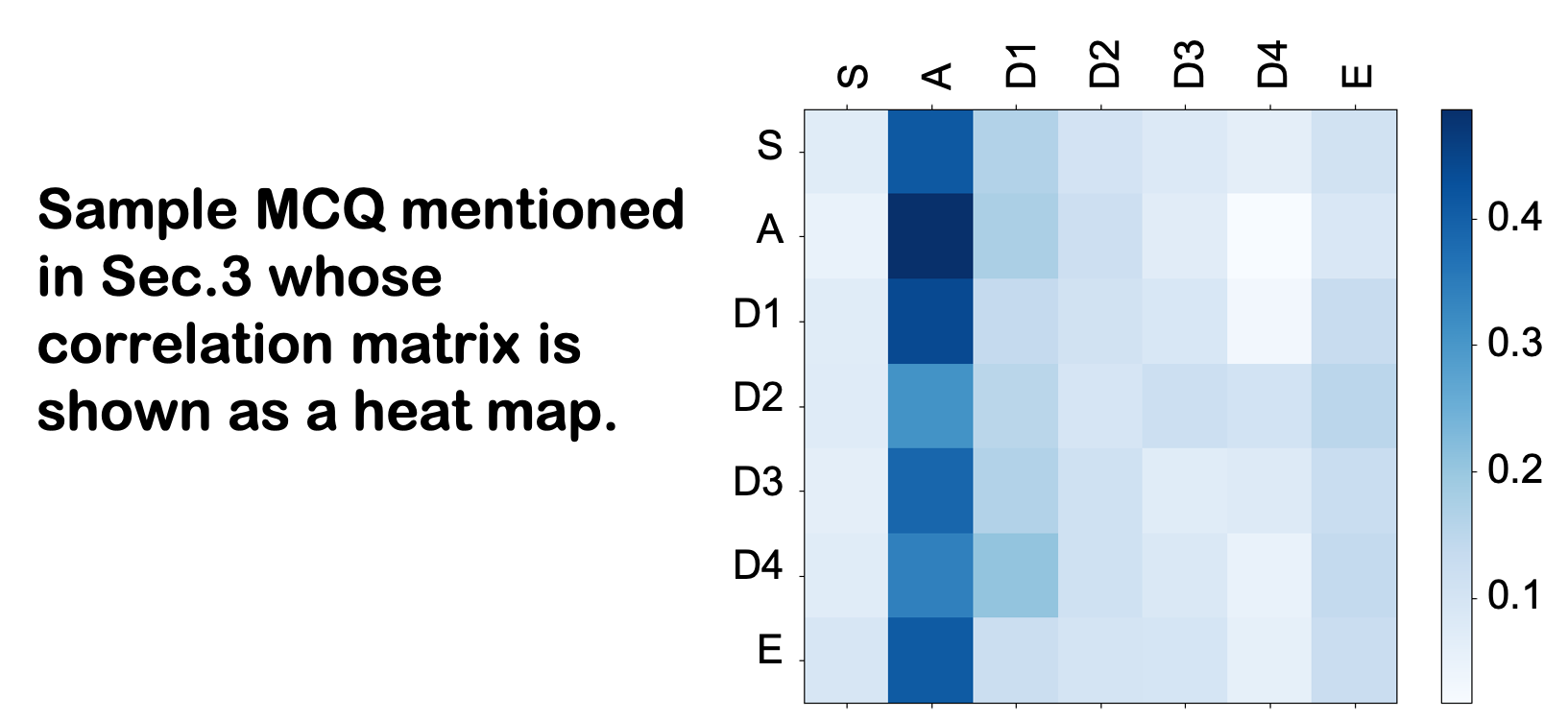
Figure 5: Visualisation of SCQC attention matrix.

Comparison of rating distributions. Fig. 6 compares the four rating distributions on M3 dataset as a case study: ground truth, $\mathsf{EDF\mathchar 45\relax Solo}$, $\mathsf{SF}$, and $\mathsf{DeepQR}$ predictions. The histogram displays the number of questions whose ratings fall within different intervals. While ratings produced by $\mathsf{EDF\mathchar 45\relax Solo}$ are too evenly distributed, and those by $\mathsf{SF}$ concentrate too much in one rating interval, the rating distribution obtained by $\mathsf{DeepQR}$ strikes a balance between the two and most resembles the ground truth.

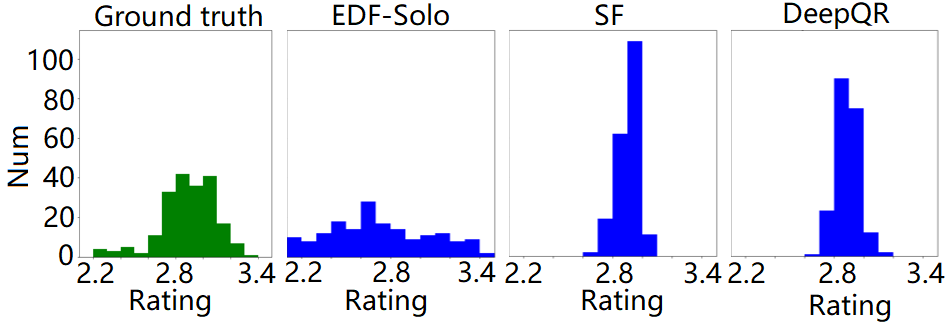
Figure 6: Ground truth and prediction distributions on M3.

Identifying questions with high- (low-)quality. A model that can detect questions with exceptionally low or high quality could be used as either a question filter (to eliminate low-quality questions) or a question recommender (to promote high-quality questions). We verify these abilities for $\mathsf{DeepQR}$: Call a question “high-quality” (or “low-quality”) if its rating falls one standard deviation above (or below) the mean of its dataset. Thus, these questions account for roughly $15\%$ of total samples assuming the ratings are normally distributed. Suppose we classify a test sample by the same rule above, but according to the predicted rating. We measure classification accuracy, namely, the proportion of questions in the test set that are correctly classified as “high” or “not high”(and “low” or “not low”). See Table 5: the results show that $\mathsf{DeepQR}$ achieves reasonably high classification accuracy for both types of questions over all datasets.

Table 5: Classification accuracy (%) for high- and low-quality questions by $\mathsf{DeepQR}$.

Cl. ACC	Law	M1	M2	M3	M4	M5	M6	M7
Low	76.30	83.42	80.79	77.83	80.99	85.06	84.80	83.51
High	75.78	82.85	87.41	84.23	88.42	80.55	80.80	86.81

Error analysis.

Although $\mathsf{DeepQR}$ achieves superior performance than other models, it nevertheless predicts falsely on many MCQs. In particular, the performance on the Law dataset is considerably worse than on other datasets. Many factors potentially contribute to this (see Table 2): (1) Law has the lowest number of ratings per MCQ (18.97) which casts a doubt on its reliability. (2) Question stems in Law have the shortest average character-level length (101.75) which could affect performance. (3) A larger proportion of MCQs in Law are numerical (e.g. on taxation).

Another potential source of inaccuracies to our model lies in the MCQ representations. Fig. 7 visualises the GloVe and QDQE question embeddings of 50 questions from M1. While it is apparent that QDQE results in a strengthened clustering effect (e.g. highly rated purple points tend to cluster in the upper right quadrant while poorly-rated red and green points cluster on the left), the resulting clustering is not entirely determined by rating categories. This shows that QDQE alone is not sufficient to capture quality rating, which is not surprising as this way of obtaining question embeddings does not account for contents in the entire course.

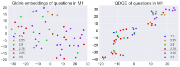
Figure 7: t-SNE (Van der Maaten and Hinton 2008) embedding visualization of GloVe (left) and QDQE (right) where points are questions and colours indicate rating categories.

6 Conclusions and Future Work

This paper investigates AQQR using tools from deep learning. We propose the $\mathsf{DeepQR}$ model that combines EDF and SF sources extracted by transformer networks, as well as contrastive learning-based question embeddings. Empirical results using eight PeerWise datasets validate the superior performance of $\mathsf{DeepQR}$ over six comparative models. Future work includes improving the model’s accuracy through better question embedding schemes and incorporating domain-specific knowledge. In addition, when training our model we aim to improve the quality of the input data (aggregated student ratings) using effective consensus approaches (Abdi et al. 2021; Darvishi, Khosravi, and Sadiq 2021). Finally, we aim to evaluate the use of $\mathsf{DeepQR}$ in practice for recommending high-quality questions to students who are engaged in practice tasks.

References

- Abdi et al. (2021) Abdi, S.; Khosravi, H.; Sadiq, S.; and Demartini, G. 2021. Evaluating the Quality of Learning Resources: A Learnersourcing Approach. IEEE Transactions on Learning Technologies, 14(1): 81–92.
- Bates et al. (2014) Bates, S. P.; Galloway, R. K.; Riise, J.; and Homer, D. 2014. Assessing the Quality of a Student-generated Question Repository. Physical Review Special Topics-Physics Education Research, 10(2): 020105.
- Bommasani et al. (2021) Bommasani, R.; Hudson, D. A.; Adeli, E.; Altman, R.; Arora, S.; von Arx, S.; Bernstein, M. S.; Bohg, J.; Bosselut, A.; Brunskill, E.; et al. 2021. On the opportunities and risks of foundation models. arXiv:2108.07258.
- Brown et al. (2021) Brown, G. T. L.; Denny, P.; San Jose, D. L.; and Li, E. 2021. Setting Standards With Multiple-Choice Tests: A Preliminary Intended-User Evaluation of SmartStandardSet. Frontiers in Education, 6: 1–17.
- Carrier and Pashler (1992) Carrier, M.; and Pashler, H. 1992. The Influence of Retrieval on Retention. Memory & Cognition, 20(6): 633–642.
- Chen et al. (2020) Chen, T.; Kornblith, S.; Norouzi, M.; and Hinton, G. 2020. A Simple Framework for Contrastive Learning of Visual Representations. In ICML 2020, 1597–1607. PMLR.
- Choi, Land, and Turgeon (2005) Choi, I.; Land, S. M.; and Turgeon, A. J. 2005. Scaffolding Peer-questioning Strategies to Facilitate Metacognition During Online Small Group Discussion. Instructional science, 33(5): 483–511.
- Crutcher and Healy (1989) Crutcher, R. J.; and Healy, A. F. 1989. Cognitive Operations and the Generation Effect. Journal of Experimental Psychology: Learning, Memory, and Cognition, 15(4): 669.
- Darvishi, Khosravi, and Sadiq (2021) Darvishi, A.; Khosravi, H.; and Sadiq, S. 2021. Employing Peer Review to Evaluate the Quality of Student Generated Content at Scale: A Trust Propagation Approach. In L@S 2021, 139–150.
- Davis et al. (2018) Davis, D.; Chen, G.; Hauff, C.; and Houben, G.-J. 2018. Activating Learning at Scale: A Review of Innovations in Online Learning Strategies. Computers & Education, 125: 327–344.
- Denny, Luxton-Reilly, and Hamer (2008) Denny, P.; Luxton-Reilly, A.; and Hamer, J. 2008. The PeerWise System of Student Contributed Assessment Questions. In ACE 2008, 69–74. Citeseer.
- Denny et al. (2011) Denny, P.; Luxton-Reilly, A.; Tempero, E.; and Hendrickx, J. 2011. CodeWrite: Supporting Student-Driven Practice of Java. In SIGCSE 2011, SIGCSE ’11, 471–476. New York, NY, USA: Association for Computing Machinery. ISBN 9781450305006.
- Devlin et al. (2019) Devlin, J.; Chang, M.-W.; Lee, K.; and Toutanova, K. 2019. BERT: Pre-training of Deep Bidirectional Transformers for Language Understanding. In NAACL-HLT 2019, 4171–4186. Minneapolis, Minnesota: Association for Computational Linguistics.
- Dhawan (2020) Dhawan, S. 2020. Online Learning: A Panacea in the Time of COVID-19 Crisis. Journal of Educational Technology Systems, 49(1): 5–22.
- DuBay (2004) DuBay, W. H. 2004. The Principles of Readability. Impact Information.
- Ebersbach, Feierabend, and Nazari (2020) Ebersbach, M.; Feierabend, M.; and Nazari, K. B. B. 2020. Comparing the Effects of Generating Questions, Testing, and Restudying on Students’ Long-Term Recall in University Learning. Applied Cognitive Psychology, 34(3): 724–736.
- Galloway and Burns (2015) Galloway, K. W.; and Burns, S. 2015. Doing It for Themselves: Students Creating a High Quality Peer-learning Environment. Chemistry Education Research and Practice, 16(1): 82–92.
- Giorgi et al. (2021) Giorgi, J.; Nitski, O.; Wang, B.; and Bader, G. 2021. DeCLUTR: Deep Contrastive Learning for Unsupervised Textual Representations. In ACL-IJCNLP 2021, 879–895. Online: Association for Computational Linguistics.
- Gunel et al. (2021) Gunel, B.; Du, J.; Conneau, A.; and Stoyanov, V. 2021. Supervised Contrastive Learning for Pre-trained Language Model Fine-tuning. In ICLR 2021. OpenReview.net.
- He et al. (2020) He, K.; Fan, H.; Wu, Y.; Xie, S.; and Girshick, R. B. 2020. Momentum Contrast for Unsupervised Visual Representation Learning. In CVPR 2020, 9726–9735. IEEE.
- Huang et al. (2017) Huang, Z.; Liu, Q.; Chen, E.; Zhao, H.; Gao, M.; Wei, S.; Su, Y.; and Hu, G. 2017. Question Difficulty Prediction for READING Problems in Standard Tests. In AAAI 2017.
- Kang (2016) Kang, S. H. K. 2016. Spaced Repetition Promotes Efficient and Effective Learning: Policy Implications for Instruction. Policy Insights from the Behavioral and Brain Sciences, 3(1): 12–19.
- Khosravi, Kitto, and Williams (2019) Khosravi, H.; Kitto, K.; and Williams, J. J. 2019. RiPPLE: A Crowdsourced Adaptive Platform for Recommendation of Learning Activities. Journal of Learning Analytics, 6(3): 91–105.
- Kim (2015) Kim, J. 2015. Learnersourcing: Improving Learning with Collective Learner Activity. Ph.D. thesis, Massachusetts Institute of Technology.
- Kim, Miller, and Gajos (2013) Kim, J.; Miller, R. C.; and Gajos, K. Z. 2013. Learnersourcing Subgoal Labeling to Support Learning from How-to Videos. In CHI 2013, CHI EA ’13, 685–690. New York, NY, USA: Association for Computing Machinery. ISBN 9781450319522.
- Kingma and Ba (2015) Kingma, D. P.; and Ba, J. 2015. Adam: A Method for Stochastic Optimization. In Bengio, Y.; and LeCun, Y., eds., ICLR 2015.
- Leinonen, Pirttinen, and Hellas (2020) Leinonen, J.; Pirttinen, N.; and Hellas, A. 2020. Crowdsourcing Content Creation for SQL Practice. In ITiCSE 2020, 349–355.
- Liu et al. (2019) Liu, Y.; Ott, M.; Goyal, N.; Du, J.; Joshi, M.; Chen, D.; Levy, O.; Lewis, M.; Zettlemoyer, L.; and Stoyanov, V. 2019. RoBERTa: A Robustly Optimized BERT Pretraining Approach. arXiv:1907.11692.
- Malau-Aduli et al. (2014) Malau-Aduli, B. S.; Assenheimer, D.; Choi-Lundberg, D.; and Zimitat, C. 2014. Using Computer-based Technology to Improve Feedback to Staff and Students on MCQ Assessments. Innovations in Education and Teaching International, 51(5): 510–522.
- McQueen et al. (2014) McQueen, H. A.; Shields, C.; Finnegan, D.; Higham, J.; and Simmen, M. 2014. PeerWise Provides Significant Academic Benefits to Biological Science Students Across Diverse Learning Tasks, but with Minimal Instructor Intervention. Biochemistry and Molecular Biology Education, 42(5): 371–381.
- Mitros (2015) Mitros, P. 2015. Learnersourcing of Complex Assessments. In L@S 2015, L@S ’15, 317–320. New York, NY, USA: Association for Computing Machinery. ISBN 9781450334112.
- Moore, Nguyen, and Stamper (2021) Moore, S.; Nguyen, H. A.; and Stamper, J. 2021. Examining the Effects of Student Participation and Performance on the Quality of Learnersourcing Multiple-Choice Questions, 209–220. New York, NY, USA: Association for Computing Machinery. ISBN 9781450382151.
- Moseley, Bonner, and Ibey (2016) Moseley, C.; Bonner, E.; and Ibey, M. 2016. The Impact of Guided Student-Generated Questioning on Chemistry Achievement and Self-Efficacy of Elementary Preservice Teachers. European Journal of Science and Mathematics Education, 4(1): 1–16.
- Naber (2003) Naber, D. 2003. A Rule-Based Style and Grammar Checker. GRIN Verlag. ISBN 9783640065769.
- Oord, Li, and Vinyals (2018) Oord, A. v. d.; Li, Y.; and Vinyals, O. 2018. Representation Learning with Contrastive Predictive Coding. arXiv preprint arXiv:1807.03748.
- Papinczak et al. (2012) Papinczak, T.; Peterson, R.; Babri, A. S.; Ward, K.; Kippers, V.; and Wilkinson, D. 2012. Using Student-Generated Questions for Student-Centred Assessment. Assessment & Evaluation in Higher Education, 37(4): 439–452.
- Pennington, Socher, and Manning (2014) Pennington, J.; Socher, R.; and Manning, C. 2014. GloVe: Global Vectors for Word Representation. In EMNLP 2014, 1532–1543. Doha, Qatar: Association for Computational Linguistics.
- Pirttinen et al. (2018) Pirttinen, N.; Kangas, V.; Nikkarinen, I.; Nygren, H.; Leinonen, J.; and Hellas, A. 2018. Crowdsourcing Programming Assignments with CrowdSorcerer. In ITiCSE 2018, 326–331.
- Qiu, Wu, and Fan (2019) Qiu, Z.; Wu, X.; and Fan, W. 2019. Question Difficulty Prediction for Multiple Choice Problems in Medical Exams. In CIKM 2019, 139–148.
- Reimers and Gurevych (2019) Reimers, N.; and Gurevych, I. 2019. Sentence-BERT: Sentence Embeddings using Siamese BERT-Networks. In EMNLP-IJCNLP 2019, 3982–3992. Hong Kong, China: Association for Computational Linguistics.
- Riggs, Kang, and Rennie (2020) Riggs, C. D.; Kang, S.; and Rennie, O. 2020. Positive Impact of Multiple-Choice Question Authoring and Regular Quiz Participation on Student Learning. CBE—Life Sciences Education, 19(2): ar16. PMID: 32357094.
- Roediger III and Karpicke (2006) Roediger III, H. L.; and Karpicke, J. D. 2006. Test-Enhanced Learning: Taking Memory Tests Improves Long-Term Retention. Psychological science, 17(3): 249–255.
- Shermis and Burstein (2003) Shermis, M. D.; and Burstein, J. C. 2003. Automated Essay Scoring: A Cross-Disciplinary Perspective. Routledge.
- Shinahara and Takehara (2020) Shinahara, Y.; and Takehara, D. 2020. Quality Assessment of Diagnostic Questions Based on Multiple Features.
- Taghipour and Ng (2016) Taghipour, K.; and Ng, H. T. 2016. A Neural Approach to Automated Essay Scoring. In EMNLP 2016, 1882–1891. Austin, Texas: Association for Computational Linguistics.
- The Machine Learning Team, TAL Education Group, Beijing, China (2020) The Machine Learning Team, TAL Education Group, Beijing, China. 2020. Solution For NeurIPS Education Challenge 2020 from TAL ML Team.
- Uto, Xie, and Ueno (2020) Uto, M.; Xie, Y.; and Ueno, M. 2020. Neural Automated Essay Scoring Incorporating Handcrafted Features. In COLING 2020, 6077–6088.
- Van der Maaten and Hinton (2008) Van der Maaten, L.; and Hinton, G. 2008. Visualizing Data Using t-SNE. Journal of machine learning research, 9(11).
- Vaswani et al. (2017) Vaswani, A.; Shazeer, N.; Parmar, N.; Uszkoreit, J.; Jones, L.; Gomez, A. N.; Kaiser, L.; and Polosukhin, I. 2017. Attention is All you Need. In Guyon, I.; von Luxburg, U.; Bengio, S.; Wallach, H. M.; Fergus, R.; Vishwanathan, S. V. N.; and Garnett, R., eds., NeurIPS 2017, 5998–6008.
- Walsh et al. (2018) Walsh, J. L.; Harris, B. H. L.; Denny, P.; and Smith, P. 2018. Formative Student-Authored Question Bank: Perceptions, Question Quality and Association with Summative Performance. Postgraduate Medical Journal, 94(1108): 97–103.
- Wang et al. (2019) Wang, X.; Talluri, S. T.; Rose, C.; and Koedinger, K. 2019. UpGrade: Sourcing Student Open-Ended Solutions to Create Scalable Learning Opportunities. In L@S 2019, L@S ’19. New York, NY, USA: Association for Computing Machinery. ISBN 9781450368049.
- Wang et al. (2020) Wang, Z.; Lamb, A.; Saveliev, E.; Cameron, P.; Zaykov, Y.; Hernández-Lobato, J. M.; Turner, R. E.; Baraniuk, R.; Barton, C.; Jones, S. L. P.; Woodhead, S.; and Zhang, C. 2020. Results and Insights from Diagnostic Questions: The NeurIPS 2020 Education Challenge. In NeurIPS 2020.
- Wolf et al. (2019) Wolf, T.; Debut, L.; Sanh, V.; Chaumond, J.; Delangue, C.; Moi, A.; Cistac, P.; Rault, T.; Louf, R.; Funtowicz, M.; et al. 2019. Huggingface’s Transformers: State-of-the-Art Natural Language Processing. arXiv preprint arXiv:1910.03771.