Ferromagnetic and metamagnetic transitions in itinerant electron systems: a microscopic study

Abstract

We perform a microscopic study of itinerant ferromagnetic systems. We reveal a very rich phase diagram in the three-dimensional space spanned by the chemical potential, a magnetic field, and temperature beyond the Landau theory analyzed so far. Besides a generic wing structure near a tricritical point upon introducing the magnetic field, we find that an additional wing can be generated close to a quantum critical end point (QCEP) and also even from deeply inside the ferromagnetic phase. A tilting of the wing controls the entropy jump associated with the metamagnetic transition. Ferromagnetic and metamagnetic transitions are usually accompanied by a Lifshitz transition at low temperatures, i.e., a change of Fermi surface topology including the disappearance of the Fermi surface. In particular, the Fermi surface of either spin band vanishes at the QCEP. These rich phase diagrams are understood in terms of the density of states and the breaking of particle-hole symmetry in the presence of a next nearest-neighbor-hopping integral $t^{\prime}$, which is expected in actual materials. The obtained phase diagrams are discussed in a possible connection to itinerant ferromagnetic systems such as UGe₂, UCoAl, ZrZn₂, and others including materials exhibiting the magnetocaloric effect.

• December 8, 2022

1 Introduction

Itinerant metamagnetism is known as a magnetic phase transition accompanied by a discontinuous change of magnetization upon applying a magnetic field [1]. Typical examples are intermetallic compounds such as ${\rm Co(Se_{1-x}S_{x})_{2}}$ [2], ${\rm Y(Co_{1-x}Al_{x})_{2}}$ [3, 4, 5], ${\rm Lu(Co_{1-x}Al_{x})_{2}}$ [6, 7], and giant magnetocaloric effect materials such as MnAs [8], ${\rm Gd_{5}(Si_{1-x}Ge_{x})_{4}}$ [9, 10], and ${\rm MnFeP_{1-x}As_{x}}$ [9, 10]. Theoretical studies of itinerant metamagnetism have a long history [11] including an issue of first-order ferromagnetic instability [12, 13, 14]. As summarized in Refs. [1] and [15], the itinerant metamagnetic transition is expected when the density of states (DOS) $N(\epsilon)$ exhibits a positive curvature $(\frac{d^{2}N}{d\epsilon^{2}}>0)$ near the Fermi energy. This condition is easily understood in terms of the Landau free energy [15]. The free energy of the system may be expanded as

$$F(m)=a_{2}m^{2}+a_{4}m^{4}+a_{6}m^{6}-hm\,,$$ (1)

where $m$ is magnetization and $h$ is a magnetic field. The large DOS usually leads to a relatively small value of $a_{2}(>0)$ and the positive curvature of the DOS can yield a negative value of $a_{4}$. In general, it is possible to find a parameter region, where $a_{6}$ is positive. Hence the Landau free energy with $h=0$ can have two local minima at $m=m_{1}(=0)$ and $m_{2}(>m_{1})$ in a positive region of $m$. We suppose a situation of $F(m_{1})<F(m_{2})$, i.e., a paramagnetic phase. In this case, upon applying a field $h$, $F(m_{1})$ becomes lower with a finite $m_{1}$, but $F(m_{2})$ is lowered more substantially. Eventually the level crossing of the two local minima occurs, leading to a first-order transition from a state with $m_{1}$ to that with $m_{2}$, which describes a metamagnetic transition.

This basic concept was developed by considering the renormalization of the coefficients $a_{2}$, $a_{4}$, and $a_{6}$ in Eq. (1) by magnetic fluctuations [16], where the temperature dependence of the bare coefficients was discarded. In particular, a phase diagram was constructed by using the renormalized coefficients of the Landau free energy Eq. (1) [17, 18]. The ferromagnetic phase transition is second order at high temperatures and changes to a first order at low temperatures, whereas the metamagnetic transition takes place above the first-order transition temperature by applying a magnetic field. Detailed comparisons with experiments were made for various metamagnetic materials such as ${\rm Co(Se_{1-x}S_{x})_{2}}$ [17, 18, 19], ${\rm Y(Co_{1-x}Al_{x})_{2}}$ [17, 18, 20, 21], ${\rm Lu(Co_{1-x}Ga_{x})_{2}}$ [17, 18], ${\rm La(Fe_{x}Si_{1-x})_{13}}$ [18], UCoAl [17], ${\rm MnFeP_{1-x}As_{x}}$ [18], and UGe₂ [22], and a qualitatively good agreement was concluded.

A different scenario was also proposed. Reference [23] showed that itinerant ferromagnets generally exhibit a first-order phase transition at low temperatures without invoking a large DOS. In a metallic system, there are always gapless particle-hole excitations around the Fermi surface. These excitations yield a nonanalytic term in the free energy. Such a term in turn generates a local minimum in the potential and can lead to a first-order transition at low temperatures. The transition is expected to change to a continuous one at high temperatures because the singular term is cut off by temperature. The resulting phase diagram shares many features with the conventional theory [17, 18]. A similar nonanalytic term was also obtained in Fermi liquid theory and was invoked to explain a metamagnetic transition [24]. On the other hand, it was shown that the nonanalytic term preempts the first-order ferromagnetic transition and leads to inhomogeneous states [25, 26].

The end point of a second-order transition line corresponds to a tricritical point (TCP), at which the transition becomes first order. As is well known in theory of the TCP [27, 28], first-order transition surfaces develop by applying a magnetic field and three critical lines merge together at the TCP: one is the second-order transition line at zero field and two are critical end lines (CELs) corresponding to the edges of the first-order transition surfaces in a finite field. A metamagnetic transition occurs when the system crosses the first-order transition surfaces by tuning the field.

Experimentally, a phase diagram similar to the general phase diagram associated with the TCP was observed in itinerant ferromagnetic materials such as UGe₂ [29, 30], UCoAl [31], and ZrZn₂ [32, 33]. On one hand, this observation supports the phase diagram [34] obtained in the mechanism in terms of the nonanalytic term [23]. However, we shall show in the present paper that a phase digram similar to experimental observations can also be captured by considering the large DOS with a positive curvature in line with early theoretical studies [1, 11, 12, 13, 14, 15, 16, 17, 18, 19].

We also notice that many theoretical studies were performed phenomenologically in detail [1, 11, 12, 13, 14, 15, 16, 17, 18, 19, 34, 35, 36], but microscopic studies of the itinerant metamagnetic transition are rather sparse [37, 38, 39]. In addition, the majority of the earlier studies [1, 15, 16, 17, 18, 19, 34, 35, 36] is based on Landau expansion, which is valid only for a small magnetization. However, a metamagnetic transition is accompanied by a large change of the magnetization and it is not clear how reliable those works are, requiring a microscopic analysis without Landau expansion. Moreover, a giant magnetocaloric effect is currently an important topic aiming to develop magnetic refrigeration [40], which will achieve high energy efficiency and will be used for hydrogen liquefaction [41]. In this respect, a metamagnetic phase transition attracts much interest because of a possibly considerable entropy change [42]. Hence it should be also valuable to establish a canonical phase diagram of itinerant ferromagnetism as well as metamagnetism.

In this paper, we introduce a microscopic mean-field exact model of itinerant ferromagnetism on a square lattice in Sec. 2. We then perform comprehensive calculations to establish three-dimensional phase diagrams spanned by temperature, the chemical potential, and a magnetic field in Sec. 3, which is beyond the scope of the Landau theory analyzed previously [1, 15, 16, 17, 18, 19]. The key advantage of the present microscopic analysis over phenomenological studies [11, 12, 13, 14, 34, 35, 36] is that we can elucidate not only the generic wing structure associated with the metamagnetic transition near a TCP, but also additional wings developing near a quantum critical end point (QCEP) and also from deeply inside the ferromagnetic phase. On top of these important findings, the present work clarifies the microscopic origin of the wing, the microscopic reason of the occurrence of the QCEP, the relation to the entropy jump, the connection to a Lifshitz transition, and the importance of a next nearest-neighbor-hopping integral $t^{\prime}$. In Sec. 4, we discuss the obtained results from both theoretical and experimental viewpoints. In particular, our obtained phase diagrams capture characteristic features observed in UGe₂ [29, 30], UCoAl [31], and ZrZn₂ [32, 33].

2 Model and Formalism

To elucidate the typical phase diagram of itinerant ferromagnetism including the effect of the Zeeman field, we study the following mean-field exact Hamiltonian on a square lattice:

$$\mathcal{H}=\sum_{{\bf k},\sigma}\xi_{{\bf k}}^{0}c_{{\bf k}\sigma}^{\dagger}c_{{\bf k}\sigma}-\frac{g}{2N}\sum_{{\bf k}{\bf k}^{\prime}\sigma\sigma^{\prime}}\sigma\sigma^{\prime}c_{{\bf k}\sigma}^{\dagger}c_{{\bf k}\sigma}c_{{\bf k}^{\prime}\sigma^{\prime}}^{\dagger}c_{{\bf k}^{\prime}\sigma^{\prime}}-\frac{h}{2}\sum_{{\bf k}\sigma}\sigma c_{{\bf k}\sigma}^{\dagger}c_{{\bf k}\sigma}\,,$$ (2)

where $c_{{\bf k}\sigma}^{\dagger}$ and $c_{{\bf k}\sigma}$ are the creation and annihilation operators for electron with momentum ${\bf k}$ and spin orientation $\sigma(=1\;{\rm or}\;-1)$, respectively; $N$ is the total number of the lattice sites. The first term is a kinetic term of electrons and its dispersion is given by

$$\xi_{{\bf k}}^{0}=-2t(\cos k_{x}+\cos k_{y})-4t^{\prime}\cos k_{x}\cos k_{y}-\mu\,.$$ (3)

Here $t$ and $t^{\prime}$ are hopping integrals between the nearest-neighbor and next nearest-neighbor sites, respectively, and $\mu$ is the chemical potential. The second term in Eq. (2) is the same as the Landau interaction function in the $s$-wave spin-antisymmetric channel [43]. It describes a spin-dependent forward scattering interaction and can lead to ferromagnetism for $g>0$. The interaction is considered only for the spin quantization axis parallel to the $z$-axis. Hence the present magnetic interaction is expected to describe an itinerant ferromagnetic system with a strong spin anisotropy observed in several U-based materials [31, 44]. Our interaction may also be applicable to a system with spin rotational invariance by considering that our interaction is obtained after a mean-field approximation to a certain microscopic model. For example, if one starts with the Hubbard interaction $U\sum_{i}c^{\dagger}_{i\uparrow}c_{i\uparrow}c^{\dagger}_{i\downarrow}c_{i\downarrow}$ where $i$ represents the lattice site, one obtains $g=U/2$ in momentum space by assuming a ferromagnetic mean-field solution, namely by focusing on the zero-momentum transfer channel—the forward scattering channel. In fact, it is well recognized in the Hubbard model that the ferromagnetic interaction actually becomes dominant when $|t^{\prime}/t|$ is relatively large around $0.3-0.5$ for the density around van Hove filling; otherwise, antiferromagnetism and $d$-wave superconductivity would be stabilized [45, 46, 47]. Respecting this insight, one might choose a large $t^{\prime}$ in our model, although a choice of our parameters is arbitrary in Eq. (2) in principle. Note that ferromagnetism is stabilized around van Hove filling also in the present model as we shall see in Sec. 3. The third term is the Zeeman energy and $h$ is an effective magnetic field defined as $h=\mathfrak{g}\mu_{B}H$, where $\mathfrak{g}$ is a $g$ factor, $\mu_{B}$ the Bohr magneton, and $H$ a magnetic field.

Other terms not included in our Hamiltonian may be present in real materials. Our interest lies in the case where ferromagnetism becomes a leading instability. Hence the Hamiltonian, Eq. (2), should be regarded as an effective minimal model in the low-energy region, which may describe a system close to ferromagnetic instability such as UGe₂ [29, 30, 44], UCoAl [31], ZrZn₂ [32, 33], and UCoGe [48].

The Hamiltonian, Eq. (2), considers the electron-electron interaction only for the forward scattering interaction of electrons. This means that fluctuations around a mean field vanish in the limit of $N\rightarrow\infty$, indicating that a mean-field theory can solve the model [Eq. (2)] exactly in the thermodynamic limit. We then decouple the interaction by introducing the magnetization

$$m=\frac{g}{2N}\sum_{{\bf k}\sigma}\sigma\langle c_{{\bf k}\sigma}^{\dagger}c_{{\bf k}\sigma}\rangle\,.$$ (4)

The resulting mean-field Hamiltonian is given by

$$\mathcal{H}_{\rm MF}=\sum_{{\bf k}\sigma}\xi_{{\bf k}\sigma}c_{{\bf k}\sigma}^{\dagger}c_{{\bf k}\sigma}+\frac{2N}{g}m^{2}\,,$$ (5)

where $\xi_{{\bf k}\sigma}=\xi_{{\bf k}}^{0}-\frac{\sigma}{2}(4m+h)$. The grand canonical potential per lattice site is computed at temperature $T$ as

$$\omega=-\frac{T}{N}\sum_{{\bf k}\sigma}\log(1+{\rm e}^{-\xi_{{\bf k}\sigma}/T})+\frac{2m^{2}}{g}\,.$$ (6)

By minimizing the potential with respect to $m$, we obtain the self-consistency equation

$$m=\frac{g}{2N}\sum_{{\bf k}\sigma}\sigma f(\xi_{{\bf k}\sigma})\,,$$ (7)

where $f(x)=({\rm e}^{x/T}+1)^{-1}$ is the Fermi distribution function.

In the presence of a magnetic field, the magnetization $m$ can exhibit a jump, i.e., a metamagnetic phase transition. The end point of the metamagnetic phase transition is called a critical end point (CEP) and is given by the condition $\left.\frac{\partial h}{\partial m}\right|_{\mu,T}=\left.\frac{\partial^{2}h}{\partial m^{2}}\right|_{\mu,T}=0$:

$$\frac{1}{g}=-\frac{1}{N}\sum_{{\bf k}\sigma}f^{\prime}(\xi_{{\bf k}\sigma})\,,$$ (8)

$$0=\frac{1}{N}\sum_{{\bf k}\sigma}\sigma f^{\prime\prime}(\xi_{{\bf k}\sigma})\,.$$ (9)

Here $f^{\prime}$ and $f^{\prime\prime}$ mean the first and second derivative with respect to $\xi_{{\bf k}\sigma}$. The CEP is determined by solving the coupled equations Eqs. (7), (8), and (9). In the limit of $m\rightarrow 0$ at $h=0$, Eq. (7) is reduced to Eq. (8); the coupled equations Eqs. (8) and (9) then determine a TCP at $h=0$.

We also study the entropy associated with a metamagnetic transition to get insight into a magnetocaloric effect. It is straightforward to compute the entropy from $S=-\frac{\partial\omega}{\partial T}|_{\mu,h}$,

$$S=\frac{1}{N}\sum_{{\bf k}\sigma}\log(1+{\rm e}^{-\xi_{{\bf k}\sigma}/T})+\frac{1}{TN}\sum_{{\bf k}\sigma}\xi_{{\bf k}\sigma}f(\xi_{{\bf k}\sigma})\,.$$ (10)

3 Results

In the present model [Eq. (2)] we have two parameters, the next nearest-neighbor integral $t^{\prime}$ and the interaction strength $g$, and three variables, temperature $T$, the chemical potential $\mu$, and a magnetic field $h$. The presence of $t^{\prime}$ breaks a particle-hole symmetry, which generates rich phase diagrams as we shall show below. We choose $t^{\prime}/t=0.35$ [49, 50], which was employed to discuss a nearly ferromagnetic compound Sr₃Ru₂O₇ (Ref. [51]) in the context of the interplay of ferromagnetism and electronic nematic order [52]. If the nematic interaction is set to zero, the model in Ref. [52] would be reduced to the present model. We shall also present results for $t^{\prime}=0$ to highlight the importance of $t^{\prime}$. As a value of $g$, we consider various choices. We scan all three variables $T$, $\mu$, and $h$, and establish the phase diagram of ferromagnetic and metamagnetic transitions. While $h$ is usually very small compared to the scale of $t$ in experiments, we wish to clarify the whole phase diagram by considering $h$ as a free variable, because we are interested in getting insight into the qualitative feature of ferromagnetic and metamagnetic phase transitions by considering the simplicity of the present model [Eq. (2)]. Obtained phase diagrams are symmetric with respect to the axis of $h=0$ and thus we study only the region $h\geq 0$. We measure all quantities with the dimension of energy in units of $t$ and put $t=1$.

3.1 Typical phase diagram

Figure 1 is the obtained phase diagram in the three-dimensional space spanned by $T$, $\mu$, and $h$. First we focus on the axis of $h=0$, where the phase diagram is shown in black. The ferromagnetic instability forms a dome-shaped phase transition line around van Hove filling $\mu_{\rm vH}=4t^{\prime}=1.4$. The phase transition is of second order along the top of the dome and is of first order on the edges. The end points of the second-order transition line are TCPs.

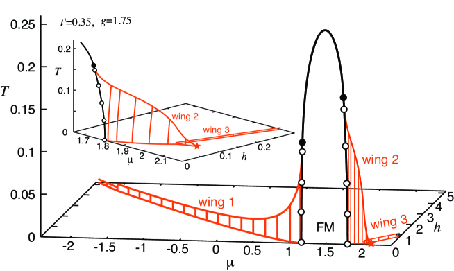
Figure 1: Phase diagram in the $\mu$-$h$-$T$ space obtained for $t^{\prime}=0.35$ and $g=1.75$. The ferromagnetic phase is realized in $1.17\leq\mu\leq 1.81$ at $h=0$; the black line and the lines with open circles denote a second-order transition and first-order transitions, respectively, and the end points of the second-order transition line are TCPs (solid circles). Two wings, wing 1 and wing 2, develop from the first-order transition lines upon applying $h$ and the wing 2 vanishes at a QCEP denoted by the star. The wing 3 develops from the wing 2 at low $T$. The wings 2 and 3 are magnified in the inset. The upper edge of the wing corresponds to the CEL. The metamagnetic transition occurs by crossing the wings.

When a field is applied, magnetization becomes finite and a ferromagnetic phase transition cannot be second order. Instead wing structures appear as shown in orange in Fig. 1. Two wings develop from the first-order transition lines at $h=0$ and describe first-order transition surfaces for a finite $h$. We refer to the wing on the side of the small (large) $\mu$ as the wing 1 (wing 2). In addition, another wing also develops from the wing 2 at low temperatures [53], which we call the wing 3; the wings 2 and 3 are magnified in the inset of Fig. 1. These wings are located close to van Hove filling of either spin band in the presence of a field. Recalling the symmetry of $h\leftrightarrows-h$, six wings are realized in the $\mu$-$h$-$T$ space. The upper edge of the wing corresponds to a CEL, which is nothing less than a set of CEPs.

To see the wing structure more precisely, we project it on the $\mu$-$T$ plane and also $\mu$-$h$ plane in Figs. 2(a)-(c) for the wing 1, 2, and 3, respectively. First we focus on Fig. 2(a). The projection on the $\mu$-$T$ plane indicates clearly that the critical end temperature is rapidly suppressed with decreasing $\mu$, exhibits a steep change at $\mu=-2$, and becomes constant. This anomaly at $\mu=-2$ indicates a Lifshitz point [54], where the Fermi surface of the down-spin band disappears; see also Fig. 6. It is interesting to see that the wing extends even beyond $\mu=-2$ without forming a QCEP. On the other hand, the projection on the $\mu$-$h$ plane shows that the critical end field ($h_{\rm CEP}$) is almost identical with a field of the metamagnetic transition at $T=0$, indicating that the wing stands almost vertically in the whole $\mu$-region. A close look at the curve of $h_{\rm CEP}$ reveals that the slope changes abruptly at $\mu=-2$ by crossing the Lifshitz point there; see also Fig. 10 where this change of the slope is more visible.

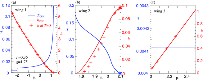
Figure 2: Projection of the wing 1 (a), wing 2 (b) and wing 3 (c) in Fig. 1 on the $\mu$-$T$ (left axis in blue) and $\mu$-$h$ (right axis in red) planes. $T_{\rm CEP}$ and $h_{\rm CEP}$ describe CELs and the symbol + denotes the position of the wing at $T=0$. The symbol star in (b) indicates a QCEP. $T_{\rm CEP}(=0.00411)$ in $\mu<-2$ in (a) is the same as that in $\mu\gtrsim 2$ in (c).

These results are easily understood. The CEP is determined by Eqs. (7), (8), and (9). Near van Hove filling, the DOS diverges logarithmically in the present model. Hence Eqs. (8) and (9) can be fulfilled around van Hove filling. This means that the wing structure is realized close to van Hove filling in the $\mu$-$h$ plane, i.e., the $\mu$-$h$ curve in Fig. 2(a) traces van Hove filling of the up-spin band in the presence of the field. Let us define the effective chemical potential as

$$\mu_{\uparrow}=\frac{4m+h}{2}+\mu\,,$$ (11)

$$\mu_{\downarrow}=-\frac{4m+h}{2}+\mu\,.$$ (12)

When the up-spin density is at van Hove filling, namely $\mu_{\uparrow}=\mu_{\rm vH}=4t^{\prime}$, we obtain $\mu_{\downarrow}=2\mu-\mu_{\rm vH}$. On the other hand, the lower band edge is given by $\mu_{L}=-4(t+t^{\prime})$. Thus when $\mu_{\downarrow}<\mu_{L}$, the down-spin band becomes fully empty: see also the DOS in Fig. 3. This condition is given by $\mu<(\mu_{L}+\mu_{\rm vH})/2=-2t=-2$, indicating that $\mu=-2$ corresponds to a Lifshitz point [54]. As long as the up-spin band is close to van Hove filling, i.e., $\mu_{\uparrow}=\mu_{\rm vH}$ even in $\mu<-2$, Eqs. (8) and (9) always have a solution at $\mu_{\uparrow}=\mu_{\rm vH}$ at the CEP, namely at $h_{\rm CEP}=2(\mu_{\rm vH}-\mu_{\rm CEP})-4m_{\rm CEP}$, where $\mu_{\rm CEP}$ and $m_{\rm CEP}$ are the chemical potential and the magnetization at the CEP, respectively. Since only the up-spin band is active around van Hove filling, $m_{\rm CEP}$ becomes constant. Similarly the critical end temperature also becomes constant to be $T_{\rm CEP}=0.00411$. Hence the CEL is described by $h_{\rm CEP}=-2\mu_{\rm CEP}+{\rm const.}$ in $\mu<-2$. This means that a QCEP cannot be present in a smaller $\mu$ region.

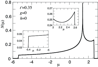
Figure 3: Density of states for $t^{\prime}=0.35$, $g=0$, and $h=0$. The insets magnify the regions close to the band edges.

Next we focus on Fig. 2(c). The projection on the $\mu$-$h$ plane shows that the CEL is located just above the line at $T=0$ with a good accuracy, that is, the wing 3 also stands vertically on the $\mu$-$h$ plane in Fig. 1. The wing 3 comes from the van Hove singularity of the down-spin band and the up-spin band is fully occupied. Hence the nature of a CEP is exactly the same as that in $\mu<-2$ in Fig. 2(a). In fact, $T_{\rm CEP}$ is the same value, there is no QCEP, and a CEP is described by $h_{\rm CEP}=2(\mu_{\rm CEP}-\mu_{\rm vH})-4m_{\rm CEP}=2\mu_{\rm CEP}+{\rm const.}$ The sign in front of $\mu_{\rm CEP}$ is opposite to the case in $\mu<-2$ because it is the down-spin band that fulfills van Hove filling for a large $\mu$. The wing 3 ends at $\mu=2.02$ by touching the wing 2 [53] as shown in Fig. 1. The proximity to the wing 2 yields a tiny enhancement of $T_{\rm CEP}$ of the wing 3 there, which is barely visible in Fig. 2(c).

Details of the wing 2 are shown in Fig. 2(b). The curve projected on the $\mu$-$h$ plane indicates that in contrast to the case of the wing 1 and wing 3, the wing 2 is tilted to the large $h$ side, especially in a small $h$ region, although it may not be so clear in Fig. 1. The temperature dependence of the CEL is characterized by two different $\mu$ regions. For $1.75\lesssim\mu\lesssim 2.0$, the effect of the van Hove singularity of the down-spin band is dominant, but the up-spin band is still involved in the DOS near the Fermi energy. This contribution is sizable because of the proximity to the band edge singularity. See the DOS in Fig. 3 with a caveat that it is computed for $h=0$ and the effective chemical potential is given by Eqs. (11) and (12) in the presence of $h$. For $2.0\lesssim\mu\lesssim 2.1$, the effect of the up-spin band becomes crucially important and we obtain two solutions satisfying Eqs. (7), (8), and (9). One solution is obtained slightly below the up-spin band edge due to thermal broadening effect. With decreasing $T$, the solution is obtained closer to the up-spin band edge and exactly there at $T=0$, leading to a QCEP. Since the Fermi surface of the up-spin band disappears at the QCEP, it is a Lifshitz point [54]. The other solution is obtained when the up-spin band is fully occupied and the effective chemical potential is located at van Hove filling of the down-spin band, yielding the wing 3 in Fig. 1 as we have already explained.

When crossing the wing, the magnetization exhibits a jump, namely a metamagnetic phase transition as shown in Fig. 4(a). The jump of the magnetization is large at low temperature, becomes smaller with increasing $T$, and vanishes at the temperature of the CEP, which corresponds to the edge of the wing in Fig. 1. The magnetic field at which the jump occurs shifts to a high field with increasing temperature in Fig. 4(a). This is because the wing 2 is tilted as shown in Fig. 2(b). Although a metamagnetic transition is usually envisaged as a first-order transition as a function of a field, the jump of the magnetism also occurs as a function of the chemical potential (density) for a fixed field as shown in Fig. 4(b). In this sense the wing structure in Fig. 1 describes a generalized metamagnetic transition. The $\mu$ scan does not cross the wing 2 above $T=0.079$, where we have a smooth change of $m$, i.e., a crossover between the large and small magnetization.

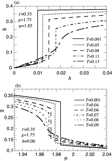
Figure 4: (a) Magnetization $m$ as a function of a magnetic field $h$ (a) and the chemical potential $\mu$ (b) for several choices of temperatures. A metamagnetic transition occurs below $T=0.122$ (a) and $T=0.079$ (b) by crossing the wing.

The entropy also exhibits a jump upon crossing the wing. The evolution of the entropy as a function of $h$ is shown in Fig. 5(a) with the same parameters as those in Fig. 4(a); results at $T=0.001$ is not shown since the entropy becomes too small to be seen in the scale of Fig. 5(a). Since the magnetization increases with increasing $h$ at each $T$ in Fig. 4(a), one might assume that the entropy should decrease with increasing $h$. However, a close look at Fig. 5(a) reveals that the entropy slightly increases upon approaching the metamagnetic transition field from below. This is easily understood intuitively. We define $\chi_{0}=-\frac{1}{N}\sum_{{\bf k}\sigma}f^{\prime}(\xi_{{\bf k}\sigma})$, which is the spin-summed DOS averaged over an energy interval of order of temperature. This quantity $\chi_{0}$ should continue to increase until the metamagnetic field because the large DOS is necessary to have a metamagnetic transition in the present model. This is indeed confirmed by the explicit calculations of $\chi_{0}$ as shown in Fig. 5(b). Recalling Boltzmann’s principle, we may associate the evolution of the entropy with that of the DOS as a function of $h$, which explains intuitively the reason why the entropy is enhanced in the vicinity of the metamagnetic transition with increasing $h$ from below in Fig. 5(a).

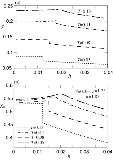
Figure 5: (a) Entropy as a function of a field $h$ for several choices of temperatures for the same parameter set as those in Fig. 4(a). (b) Similar plot for $\chi_{0}$, which is defined as the spin-summed temperature-averaged DOS.

The relation between the entropy jump and the magnetization jump at the metamagnetic transition is described by the Clapeyron equation [55]:

$$\Delta S=-\Delta M\frac{dh}{dT}\,,$$ (13)

where $\Delta S$ and $\Delta M=\Delta m/g$ are jumps of the entropy and the magnetization, respectively. The key quantity here is $\frac{dh}{dT}$, which is a derivative along the coexistence curve, is zero when the wing stands vertically on the $\mu$-$h$ plane, and becomes finite when the wing is tilted. That is, it describes how much the wing is tilted with respect to the $\mu$-$h$ plane. Consequently, the entropy jump always becomes very small upon crossing a wing when it stands almost vertically. Hence if we compute the entropy jump across the wing 1 and the wing 3 in Fig. 1, it becomes very small even at a finite $T$ although the magnetization jump is sizable. This is the reason why we have chosen the wing 2 to describe the entropy jump in Fig. 5.

At zero temperature, the entropy change becomes zero because of the third law of thermodynamics, yielding no jump of the entropy even crossing the wings. This implies $\frac{dh}{dT}=0$ at $T=0$, that is, the wing stands vertically on the $\mu$-$h$ plane in the limit of $T=0$ in Fig. 1.

In the present model, ferromagnetic and metamagnetic transitions are usually accompanied by a Lifshitz transition [54] at least at low temperatures. This is because they occur close to the van Hove singularity as well as the band edge via a first-order transition at low temperatures. There are two different types of Lifshitz transitions: i) the topology of the Fermi surface changes or ii) a Fermi surface of either up- or down-spin band disappears. The former type is observed when the metamagnetic transition occurs close to van Hove filling. Representative results are shown in Figs. 6(a) and (b). The latter type is expected when the metamagnetic transition occurs close to the band edge as shown in Figs. 6(c) and (d).

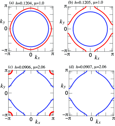
Figure 6: Fermi surfaces of the up-spin (red) and down-spin (blue) band at $T=0.0002$ for $t^{\prime}=0.35$ and $g=1.75$. (a) and (b) The topology of the up-spin Fermi surface changes by crossing the wing 1 in Fig. 1. (c) and (d) The up-spin Fermi surface disappears by crossing the wing 2 close to the QCEP in Fig. 1.

The obtained phase diagram shown in Fig. 1 is regarded as a typical one of the itinerant ferromagnetic system in the presence of a field. Generic features may be summarized as follows—quantitative features, of course, depend on details. The ferromagnetic instability occurs around van Hove filling at $h=0$ with a dome-shaped transition line. Applying the field $h$, the wing develops from the first-order transition line at $h=0$ as shown in Fig. 1. There are two important chemical potentials $\mu=-2$ and $2$, independent of $t^{\prime}$ and $g$. The value of $\mu=2$ $(-2)$ corresponds to the case, in which the down-spin (up-spin) band is located at van Hove filling and the effective chemical potential of the up-spin (down-spin) [see Eqs. (11) and (12)] sits at the upper (lower) edge of the band. Hence either spin band becomes full or empty above $|\mu|\gtrsim 2$ and only the other spin band becomes active there. As a result, the temperature and the magnetization at the CEP become constant along the CEL in $|\mu|\gtrsim 2$, which is described by $h_{\rm CEP}=2|\mu_{\rm CEP}|+{\rm const.}$ In the present two-dimensional model, the DOS (see Fig. 3) exhibits a jump at the band edges and thus a temperature of a CEP shows a rapid change at $|\mu|=2$. In particular, when the DOS is enhanced near the band edge as seen in the large $\mu$ side in Fig. 3, two wings are realized around $\mu=2$. One dominant wing develops from the first-order transition line at $h=0$ and vanishes near $\mu=2$, leading to a QCEP, and the other wing forms a rectangular shape in a region of high $h$ as shown in Fig. 1. From a viewpoint of the topology of the Fermi surface, $\mu=-2$ and the QCEP correspond to Lifshitz points, where the Fermi surface of the down- and up-spin band vanishes, respectively.

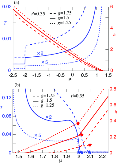
Figure 7: Projection of the CELs on the $\mu$-$T$ (left axis in blue) and $\mu$-$h$ (right axis in red) planes for several choices of $g$ in the small (a) and large (b) $\mu$ region. $T_{\rm CEP}$ for $g=1.5$ and $1.25$ is multiplied by $2$ and $5$, respectively. The CEL is not shown in the whole temperature region, but plotted only in a low-temperature region. The CEL in (a) corresponds to the wing 1. In (b) two CELs are drawn for each $g$ and describe the wing 2 and 3, respectively. A QCEP (denoted by the star) associated with the wing 2 is realized at $\mu_{\rm QCEP}=2.095,2.021$, and $2.003$ for $g=1.75,1.5$, and $1.25$, respectively. $T_{\rm CEP}$ associated with the wing 3 is the same as that in $\mu<-2$; $T_{\rm CEP}=0.0041,0.0011$ and $0.00016$ for $g=1.75,1.5$, and $1.25$, respectively.

It might seem odd that the value of $|\mu|=2$ does not depend on $g$ and a QCEP always appears close to $\mu=2$ for the positive $t^{\prime}$. This is, however, reasonable because the underlying mechanism lies in the proximity to the band edge and the enhancement of the DOS near $\mu\approx 2$ owing to the presence of $t^{\prime}$ as we have explained. To emphasize this important insight, we show in Fig. 7 how the CEL depends on $g$ by projecting it on the $\mu$-$T$ plane in blue. As expected, the temperature scale as well as the region of the ferromagnetic phase is shrunk for a smaller $g$ with keeping the qualitative features unchanged: the ferromagnetic phase is realized in $1.17\leq\mu\leq 1.81$, $1.28\leq\mu\leq 1.57$, and $1.35\leq\mu\leq 1.46$ with the maximal $T_{c}$ around $0.25$, $0.12$, and $0.046$ for $g=1.75,1.5$, and $1.25$, respectively. However, the value of $|\mu|=2$ works as a fixed point because it describes the band edge when either spin band is located at van Hove filling in the presence of a field $h$. Hence a QCEP is always realized close to $\mu\approx 2$ and the constant temperature of the CEL appears in $|\mu|\gtrsim 2$ as shown in Fig. 7. It is interesting to note that $T_{\rm CEP}$ slightly increases close to $\mu=2$ in Fig. 7(b) before vanishing at a QCEP for $g=1.5$ and $1.25$. In Fig. 7 we also present the projection of the CEL on the $\mu$-$h$ plane in red. As we have already explained, the CEL is described by $h_{\rm CEP}=-2\mu_{\rm CEP}+{\rm const.}$ in $\mu<-2$ and $h_{\rm CEP}=2\mu_{\rm CEP}+{\rm const.}$ in $\mu>2$, and thus the slope does not depend on $g$ there. Around $\mu=2$ two CELs touch to each other because the wing 3 develops from the wing 2 at low temperature as seen in Fig. 1. In particular, when $g$ becomes small, e.g., $g=1.25$ in Fig. 7(b), the wing 3 is realized very close to the QCEP associated with the wing 2. Consequently, the QCEP seems to extend as a line along the wing 3, but $T_{\rm CEP}$ is not zero along the wing 3.

3.2 Phase diagram hosting two ferromagnetic regions

We have studied generic features of the ferromagnetic and metamagnetic transitions in the itinerant electron system by taking a relatively small $g$. Some special, but interesting features are realized for a larger $g$, which we present here and also in the next subsection.

Typically one ferromagnetic phase is realized around van Hove filling at $h=0$ as we have already shown in Fig. 1. However, there is a parameter, which yields an additional ferromagnetic region at $h=0$ close to the band edge. As a representative result we choose $g=2$ and show the obtained phase diagram in Fig. 8(a); a region close to the band edge is magnified in Fig. 8(b). On top of a ferromagnetic region around van Hove filling ($\mu=1.4$), an additional ferromagnetic region emerges in $2.42\leq\mu\leq 2.6$ at $h=0$, with a first-order transition near $\mu=2.4$ and a quantum critical point (QCP) at $\mu=2.6$. This phase is due to the band edge singularity of the DOS as shown in Fig. 3, where the DOS slightly increases toward the band edge.

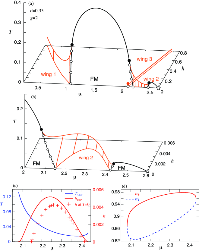
Figure 8: (a) Phase diagram in the $\mu$-$h$-$T$ space obtained for $t^{\prime}=0.35$ and $g=2$. Two ferromagnetic regions are realized in $1.04\leq\mu\leq 2.15$ and $2.42\leq\mu\leq 2.6$ at $h=0$; the black line and the lines with open circles denote a second-order transition and first-order transitions, respectively, and solid circles are TCPs and the star is a QCP. Inside the ferromagnetic phase, a metamagnetic transition occurs at $\mu=2.06$ and an orange circle denotes a CEP at $h=0$. The wing 1 develops from the first-order transition line upon applying $h$ on the small $\mu$ side and the wing 3 develops from the metamagnetic transition line at $h=0$. The first-order transitions of the two ferromagnetic regions are connected with the wing 2 through a finite $h$ region. The wing 2 is magnified in (b). (c) Projection of the wing 2 on the $\mu$-$T$ and $\mu$-$h$ planes. $T_{\rm CEP}$ and $h_{\rm CEP}$ describe the CEL and the symbol + denotes the position of the wing at $T=0$. (d) Density of the up- ($n_{\uparrow}$) and down-spin ($n_{\downarrow}$) along the CEL of the wing 2.

In this setup, a magnetic field yields a wing, referred to as the wing 2, which bridges two first-order transitions at $h=0$ through a finite $h$ region. The scale of the magnetic field is very small, indicating that the wing is realized very close to the $h=0$ line. In contrast to the case in Fig. 1, no QCEP is realized. To clarify this new wing structure, we project it on the $\mu$-$T$ planes as shown in Fig. 8(c). Interestingly, $T_{\rm CEP}$ is not monotonic as a function of $\mu$. Figure 8(c) also shows that the wing 2 is tilted substantially to the large $h$ side. In Fig. 8(d), we plot the density of each spin along the CEL of the wing 2. The system is close to the band edge, and $n_{\uparrow}$ and $n_{\downarrow}$ have $2-13$% and $4-17$% holes, respectively.

In Fig. 8(a) the metamagnetic transition line emerges at low temperatures inside the ferromagnetic phase at $\mu=2.06$ even at zero field. With applying a field, a wing structure develops with a rectangular shape. This wing originates from the van Hove singularity of the down-spin band and the underlying mechanism is the same as the wing 3 in Fig. 1. Therefore the CEL is described by $h_{\rm CEP}=2\mu_{\rm CEP}+{\rm const.}$, and $T_{\rm CEP}=0.0113$ independent of $h$.

While the wing 1 is not shown in $\mu<0.4$ in Fig. 8(a), it extends to a smaller $\mu$ with lowering $T_{\rm CEP}$. Then $T_{\rm CEP}$ decreases rapidly around $\mu=-2$ and becomes constant in $\mu<-2$, similar to the wing 1 in Fig. 1. $T_{\rm CEP}$ in $\mu\leq-2$ becomes the same temperature as $T_{\rm CEP}$ of the wing 3 in Fig. 8(a). This is because in both cases the CEP is determined by the van Hove singularity of either spin band and the other spin band is inactive.

3.3 Phase diagram for large interaction strength

The ferromagnetic regions marge into the major phase for larger interaction strength. Consequently, as shown in Fig. 9, a single ferromagnetic phase is realized at $h=0$ with a second-order transition on the large $\mu$ side, yielding a ferromagnetic QCP at the band edge at $\mu=2.6$. Inside the ferromagnetic phase, the metamagnetic transition line is realized at $\mu=2.23$ even without a field, similar to the case at $\mu=2.06$ in Fig. 8(a). Upon applying a field, a wing develops from the first-order transition line around $\mu\approx 0.7$ at $h=0$. This wing is qualitatively the same as the wing 1 in Figs. 1 and 8(a): $T_{\rm CEP}$ shows a rapid change around $\mu=-2$ and becomes constant to be $T_{\rm CEP}=0.0465$ in $\mu<-2$, where only the up-spin band is active. In contrast to Figs. 1 and 8, a wing corresponding to the wing 2 is not realized. The wing 3 is essentially the same as that in Fig. 8(a) and develops from the metamagnetic transition line at $h=0$, forming a rectangular shape, where only the down-spin band is active and thus $T_{\rm CEP}$ becomes equal to that of the wing 1 in $\mu<-2$. Since both wing 1 and wing 3 originate from the van Hove singularity of either spin band, no QCEP is realized even in a large $h$ region.

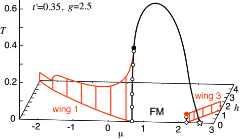
Figure 9: Phase diagram in the $\mu$-$h$-$T$ space obtained for $t^{\prime}=0.35$ and $g=2.5$. The ferromagnetic phase is realized in $0.69\leq\mu\leq 2.6$ at $h=0$; the black line and the lines with open circles denote a second-order transition and first-order transitions, respectively; the solid circle is a TCP and the star a QCP. The metamagnetic transition occurs even inside the ferromagnetic phase in low $T$ at $\mu=2.23$ and the orange circle denotes a CEP at $h=0$. Two wings develop from the first-order line and the metamagnetic transition line upon applying $h$, and are depicted by the wing 1 and wing 3, respectively. The wing 3 has $T_{\rm CEP}=0.0465$, the same value as that of the wing 1 in $\mu\lesssim-2$.

3.4 Particle-hole asymmetry

The presence of a finite $t^{\prime}$ is responsible for the rich phase diagrams shown in Figs. 1, 8, and 9. A large asymmetry with respect to van Hove filling and a metamagnetic transition even inside the ferromagnetic phase shown in Figs. 8 and 9 are in fact owing to a finite $t^{\prime}$. In particular, $t^{\prime}$ yields a slight enhancement of the DOS near the band edge on the large $\mu$ side in Fig. 3. This seemingly subtle effect gives a large impact on the phase diagram of the ferromagnetic and metamagnetic transitions such as a wing terminating with a QCEP for a finite field (Fig. 1), an additional ferromagnetic region close to the band edge (Fig. 8), and a wing connecting to two first-order transition lines (Fig. 8).

While we have presented results for $t^{\prime}>0$, similar phase diagrams would be obtained for $t^{\prime}<0$, where a wing structure on the large (small) $\mu$ side in Figs. 1, 8, and 9 are realized on the small (large) $\mu$ side. Hence a QCEP would be realized close to $\mu=-2$.

3.5 Phase diagram for $t^{\prime}=0$

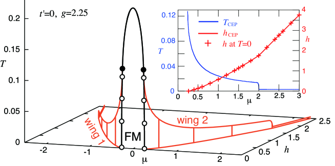
Figure 10: Phase diagram in the $\mu$-$h$-$T$ space obtained for $t^{\prime}=0$ and $g=2.25$. The ferromagnetic phase is realized in $-0.26\leq\mu\leq 0.26$ at $h=0$; the black line and the lines with open circles denote a second-order transition and first-order transitions, respectively, and solid circles are TCPs. Two wings, wing 1 and wing 2, develop from the first-order transition lines upon applying $h$. The phase diagram is symmetric with respect to $\mu=0$. The inset shows a projection of the wing 2 on the $\mu$-$T$ (left axis in blue) and $\mu$-$h$ (right axis in red) planes. $T_{\rm CEP}$ and $h_{\rm CEP}$ describe the CEL and the symbol + denotes the position of the wing at $T=0$. The CEL becomes straight in $\mu>2$, where $T_{\rm CEP}=0.0028$.

The importance of $t^{\prime}$ is highlighted by results for $t^{\prime}=0$ shown in Fig. 10. The phase diagram becomes symmetric with respect to $\mu=0$ owing to a particle-hole symmetry. A ferromagnetic phase is realized with a dome shape at $h=0$ and the transition is of first order at low temperatures. Upon applying a field, a wing structure develops along van Hove filling of either spin band. The temperature of a CEP drops at $|\mu|=2$ and concomitantly, $h_{\rm CEP}$ also changes the slope at $|\mu|=2$ as seen in the inset in Fig. 10, where the wing is projected on the $\mu$-$T$ and $\mu$-$h$ planes. The CEP is realized even in $|h|>2$ with a constant $T_{\rm CEP}(=0.0028)$, where only the either spin is active and the Fermi surface of the other spin band vanishes. Since $h_{\rm CEP}$ is practically the same as a metamagnetic field at $T=0$ as seen in the inset, the wing in Fig. 10 stands vertically on the $\mu$-$h$ plane.

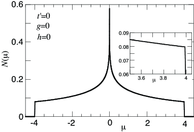
Figure 11: Density of states for $t^{\prime}=0$, $g=0$, and $h=0$. The inset magnifies a region close to the band edge.

In contrast to the cases in the presence of $t^{\prime}$, a qualitatively different feature does not appear even for changing the interaction strength $g$ at least in $g\lesssim 5$. This is easily understood by noting a shape of the DOS. As shown in Fig. 11, the DOS exhibits the van Hove singularity at $\mu=0$ and decreases monotonically upon going away from van Hove filling. Even if the chemical potential approaches the band edge, no enhancement of the DOS occurs as shown in the inset. This feature is very similar to the one on the low $\mu$ side in the presence of $t^{\prime}$ shown in Fig. 3. This explains the reason why the wing structures shown in Fig. 10 becomes similar to that on the low $\mu$ side shown in Figs. 1, 8, and 9.

4 Conclusions and discussions

4.1 Theoretical perspective

The major point of the present work is to elucidate the actual phase diagrams of ferromagnetic and metamagnetic transitions in the three-dimensional space of the chemical potential $\mu$, a magnetic field $h$, and temperature $T$ by performing a microscopic study beyond phenomenological works so far [1, 11, 12, 13, 14, 15, 16, 17, 18, 19, 34, 35, 36]. In particular, we have found that even a small enhancement of the DOS at the band edge leads to rich phase diagrams as shown in Figs. 1, 8, and 9 on the large $\mu$ side.

While we have studied a square lattice system, our obtained results can form the foundation for itinerant ferromagnetic and metamagnetic transitions in other systems. As early theoretical studies [1, 11, 12, 13, 14, 15] revealed, the large DOS with a positive curvature as a function of energy is crucial to ferromagnetic and metamagnetic transitions. In the square lattice system, such a condition is fulfilled around van Hove filling as well as the band edge in the presence of a finite $t^{\prime}$. In other systems, the microscopic origin to fulfill that condition may become different. However, we expect that resulting phase diagrams including the wing structure may not differ essentially from the present results as long as the DOS near the Fermi energy plays a crucial role. In addition, while the physics we have described is based on the band structure, the band dispersion does not necessarily mean a bare one, but can be a renormalized one, for example, obtained after a mean-field-like approximation. One would consider multi-orbital degrees of freedom as well as spin-orbit coupling important in metamagnetic materials. Given that the present simple model already leads to the complex phase diagrams, a resulting phase diagram would become highly complicated especially when several bands cross the Fermi energy and yield a large DOS relevant to a metamagnetic transition. Even in this case, the present results would offer a solid basis to construct a complicated phase diagram. On the other hand, if practically only one band yielding a large DOS crosses the Fermi energy, a phase diagram similar to the present results would be obtained—the spin degrees of freedom in the present model may be then regarded as pseudospins describing the two Kramers degenerate states in zero magnetic field.

A physics different from ours was proposed. Reference [23] showed that the low-energy particle-hole excitations, which are always present in a metallic system and independent of the band structure, generate a singular contribution to the free energy. As a result, they pointed out that a ferromagnetic order generally occurs via a first-order transition at low temperatures. Consequently, a wing structure also develops from the first-order transition line upon applying a field [34]. A resulting phase diagram becomes qualitatively similar to our results. There are, however, crucial differences, which may serve to identify the mechanism of ferromagnetic and metamagnetic transitions by considering the following: i) whether the magnetic transition is accompanied by a Lifshitz transition, ii) whether multiple wings are realized, and iii) whether a wing also develops even from the deeply inside of the ferromagnetic phase. These possibilities may not occur in general in the scenario proposed in Ref. [23] whereas they can occur in the band structure scenario. In the present model, the point i) holds in general at least at low temperatures, the point ii) also holds close to the band edge with a finite $t^{\prime}$, and the point iii) is the case for a large interaction strength with $t^{\prime}$. Those characteristic features in our model are shared to some extent with results obtained in a two-band Anderson lattice model [39], where the DOS plays an important role of the metamagnetic transition, although the DOS contains a hybridization gap in contrast to our case (Fig. 3).

The wing structure developing from a first-order transition is not a special feature of the ferromagnetic system when applying a field. In the mixture of ³He-⁴He, Griffiths pointed out the emergence of the wing structure from a first-order transition when applying a field conjugate to the superfluid density [27], although such a field cannot be controlled in experiments. In addition, similar wings were also reported by applying $xy$-anisotropy to a system where the electronic nematic instability occurs via a first-order transition in the tetragonal phase [56]. The $xy$-anisotropy can be controlled by uniaxial pressure and strain, and corresponds to a quantity conjugate to the nematic order parameter. The feature common to those three cases lies in that a TCP is present without a field and a wing is realized by applying a field conjugate to the order parameter. Referring to Griffiths’s pioneering work about the wing structure, we may call it the Griffiths wing.

We remark on the magnetocaloric effect associated with a metamagnetic transition. Although a jump of magnetization occurs upon crossing the Griffiths wing in Figs. 1, 8, 9, and 10, this does not necessarily imply a sizable magnetocaloric effect. As seen in Eq. (13), a value of $\frac{dh}{dT}$ also does matter as was already pointed out in Refs. [18] and [57]. It becomes nearly zero as long as the Griffiths wing stands almost vertically on the $\mu$-$h$ plane and exactly zero at $T=0$. A sizable magnetocaloric effect is expected only around the wing 2 in the present minimal model, where the wing is tilted toward a higher field in Figs. 1 and 8. The present work, therefore, suggests that a value of $\frac{dh}{dT}$ along the coexistence line is more crucial than the jump of the magnetization associated with a metamagnetic transition to achieve a large magnetocaloric effect in metamagnetic materials.

How about the effect of ferromagnetic fluctuations on the phase diagram? Since we have employed a purely forward scattering model, fluctuations vanish in the thermodynamic limit. Hence we need to change the interaction term in Eq. (2) to, for example, one allowing a finite momentum transfer. An analysis of the Griffiths wing associated with the electronic nematic phase transition [56] showed that fluctuations beyond mean-field calculations suppress the tendency of a first-order transition and can wash out a part of the Griffiths wing at low temperatures. We therefore infer a similar case for the ferromagnetic and metamagnetic transition. The wing 2 in Fig. 1 could be shrunk and the QCEP would be realized closer to the first-order ferromagnetic transition. This is an intriguing situation—strong fluctuations occur even near the first-order transition. Furthermore, the wing 1 could terminate with a new QCEP and the wing 3 could be fully washed out with reasonably strong fluctuations. These analyses including a resulting non-Fermi liquid state [58], metamagnetic quantum criticality [59], and possible instabilities toward various phases such as triplet superconductivity [60], spiral magnetism [25], a $d$-wave spin nematic order [25], and pair-density wave [26] are left to the future.

4.2 Experimental perspective

The effect beyond the present mean-field model is expected to be important to capture correctly the temperature dependence of the magnetic susceptibility, the specific heat, the nuclear spin relaxation rate, the resistivity, and others observed in experiments, as was extensively studied in the self-consistent renormalization theory [61]. In addition, given the minimal mean-field model [Eq. (2)], any quantitative comparison with experimental data is beyond the scope of the present work. Therefore, we wish to discuss actual ferromagnetic systems focusing on a geometrical feature of the phase diagram. Moreover, although we have elucidated phase diagrams as a function of $\mu$, namely the electron density, our $\mu$ should not be viewed as a literal meaning when making a comparison with experiments. Rather it may be interpreted as a control parameter of the phase transition to tune the DOS at the Fermi energy. For example, if the pressure is a control parameter in experiments, we may assume that the pressure controls the evolution of the DOS at the Fermi energy.

UGe₂ is one of well studied ferromagnetic metals with strong spin anisotropy [29, 30, 44]. The transition is a first order at low temperatures, from which a wing develops. The wing was reported to disappear at a QCEP. This feature is similar to our wing 2 obtained in Fig. 1. On top of that, a different wing also develops from a metamagnetic transition line inside the ferromagnetic phase (the boundary of FM1 and FM2 in Ref. [29]), similar to our results around $\mu=2.06$ and $2.23$ in Figs. 8 and 9, respectively. While the present simple model cannot capture those two features for the same interaction strength, the present work suggests the importance of the enhancement of the DOS to understand the experimental data. The two wing structures in UGe₂ were also discussed in Ref. [39] by invoking different variables in each case in a two-band Anderson lattice model.

A wing structure was also reported in UCoAl [31]. This wing was extrapolated to terminate at a QCEP. Above a field of the QCEP, a metamagnetic crossover was reported. Such data may be interpreted in two different scenarios. One scenario is that the QCEP postulated in experiments is not actually present, but the temperature of a CEL simply becomes too low, not zero, to be detected. In the present model, temperature of a CEL drops abruptly when a band of either spin becomes empty or full; see the region around $\mu=-2$ in Fig. 7(a), for instance. Another scenario is that the Griffiths wing indeed terminates at the postulated QCEP. The metamagnetic transition above the QCEP can be associated with another Griffiths wing developing from the vicinity of the QCEP as seen in Fig. 7(b). This temperature scale is, however, too low to be detected in experiments and thus the metamagnetism is observed as a crossover. In both scenarios, i) the postulated QCEP corresponds to a Lifshitz point [54] and ii) the metamagnetic crossover can be accompanied by a Lifshitz transition since the Griffiths wing is located close to van Hove filling, one of the typical features of a metamagnetic transition in terms of the large DOS.

ZrZn₂ [32, 33] is an itinerant ferromagnet and also exhibits a first-order transition at low temperatures. The above discussions about UGe₂ and UCoAl can also be applied to ZrZn₂ in the following points. First two metamagnetic transition lines associated with FM1 and FM2 are reported in Refs. [32] and [33], similar to UGe₂. In addition, the Griffiths wing was presumed to end at a QCEP, beyond which a metamagnetic crossover extends, similar to UCoAl.

The metamagnetic transition inside the ferromagnetic phase observed in UGe₂ [29] and ZrZn₂ [32, 33] was discussed in terms of a double-peak structure of the electronic DOS in Ref. [37]. In the present model, however, the metamagnetic transition inside the ferromagnetic phase around $\mu=2.06$ and $2.23$ in Figs. 8(a) and 9, respectively, originates from a single-peak structure of the DOS, namely the van Hove singularity of the down-spin band inside the ferromagnetic phase. An insight similar to ours was also obtained in Ref. [39].

Griffiths wings forming a double-wing structure were reported in LaCrGa₃ [62]. Although multiple Griffiths wings were also obtained in Figs. 1 and 8 on the large $\mu$ side, the wing 2 and wing 3 are qualitatively different from the double-wing structure observed in LaCrGa₃. Considering that LaCrGa₃ also exhibits an antiferromagnetic phase next to the ferromagnetic phase, Ref. [63] performed a phenomenological analysis by including both ferromagnetic and antiferromagnetic order parameters in the framework of the nonanalytic correction to the free energy from gapless particle-hole excitations. Obtained results successfully captured the overall phase diagram, but not the double-wing structure. It may be worthwhile to perform a microscopic analysis in a framework similar to the present work by including an antiferromagnetic interaction and see whether an important insight is obtained to understand the double Griffiths wings in LaCrGa₃.

UCoGe was reported to exhibit a first-order ferromagnetic transition at ambient pressure [48]. If a TCP is hidden on the negative pressure side, we expect the emergence of a Griffiths wing upon applying a field, as suggested by many theoretical studies [27, 28, 34, 56]. This possibility may be worth exploring further in experiments.

In the experimental literature [29, 30, 31, 32, 33, 62], the Griffiths wing is frequently assumed to end with a QCEP. This is supported theoretically by the mechanism of the nonanalytic correction from gapless particle-hole excitations around the Fermi surface [34] and also by a specific study of UGe₂ in a two-band Anderson lattice model [39]. On the other hand, from a view of the band-structure mechanism in the present simple model, the presence of a QCEP seems a delicate issue. While it is only the wing 2 in Fig. 1 that terminates with a QCEP, the other wings extend up to a high field at very low temperatures. Moreover, as discussed in the last paragraph in Sec. 4.1, the wing 1 might also yield a QCEP by order-parameter fluctuations.

Theoretical efforts [64, 65, 66, 67, 68] were made to understand the metamagnetic transition observed in ${\rm CeRu_{2}Si_{2}}$ in terms of the periodic Anderson model, where conduction electrons hybridize with the almost localized $f$ electrons. We, however, point out that ${\rm CeRu_{2}Si_{2}}$ provides a setup very different from the present model in that it is a paramagnet characterized by antiferromagnetic correlations via the RKKY interaction [69, 70], not ferromagnetic fluctuations in the vicinity of a ferromagnetic phase.

We also provide a few remarks on ${\rm Sr_{3}Ru_{2}O_{7}}$, because it exhibits a wing structure in the space of a magnetic field, tilting angle of the field, and temperature [51]. In the early days, ${\rm Sr_{3}Ru_{2}O_{7}}$ was envisaged as a system of a metamagnetic transition. However, later the dome-like phase was discovered as a function of a field, with a first-order transition at the edges of the dome. This cannot be interpreted as a usual metamagnetic phenomenon. Rather a $d$-wave Pomeranchuk instability [71, 72], i.e., the electronic nematic instability was proposed. Since the nematic transition usually occurs via a first-order transition at low temperatures [73, 74], the nematic transition as a function of a field is necessarily accompanied by a jump of the magnetization. Furthermore, the recent neutron scattering experiment [75] revealed that the nematic dome is actually the dome of an incommensurate spin-density-wave (SDW) phase with a wavevector ${\bf q}=(q_{x},0,0)$, which is in line with a Ginzburg-Landau theory [36]. It is not yet settled which is the driving force to yield the dome-like phase, the nematic instability or the SDW instability or others. More works are necessary to provide additional insight into the wing structure observed in ${\rm Sr_{3}Ru_{2}O_{7}}$.

We conclude the present work with a future perspective to understand a metamagnetic transition in metals. It is the large DOS which drives a metamagnetic transition in the present model. It is, however, likely true that effects other than the large DOS may also play a certain role in actual materials, for example, nonanalytic corrections from gapless particle-hole excitations around the Fermi energy [23] and magnetoelastic coupling [76]. In particular, the former scenario was discussed for various itinerant ferromagnets [25, 26, 34]. The latter effect was invoked to understand the large magnetocaloric effect in ${\rm MnFeP_{0.45}As_{0.55}}$ [76]. In reality, these effects as well as the DOS are expected to work constructively to yield a metamagnetic transition. Hence the crucial issue is to identify which effect is actually dominant. The present work has clarified details of itinerant metamagnetism microscopically from a viewpoint of the large DOS and will serve as a solid basis toward more complete understanding of a metamagnetic transition in metallic compounds.

References

References

- [1] Levitin R Z and Markosyan A S 1989 Sov. Phys. Usp. 31 730
- [2] Adachi K, Matsui M and Kawai M 1979 J. Phys. Soc. Jpn. 46 1474–1482
- [3] Aleksandryan V V, Lagutin A S, Levitin R Z, Markosyan A S and Snegirev V V 1985 Sov. Phys. JETP 62 153
- [4] Sakakibara T, Goto T, Yoshimura K, Shiga M and Nakamura Y 1986 Phys. Lett. A 117 243–246
- [5] Goto T, Fukamichi K, Sakakibara T and Komatsu H 1989 Solid State Commun. 72 945–947
- [6] Gabelko I L, Levitin R Z, Markosyan A S and Snegirev V V 1987 JETP Lett. 45 458
- [7] Fukamichi K, Yokoyama T, Saito H, Goto T and Yamada H 2001 Phys. Rev. B 64(13) 134401
- [8] Gama S, Coelho A A, de Campos A, Carvalho A M G, Gandra F C G, von Ranke P J and de Oliveira N A 2004 Phys. Rev. Lett. 93(23) 237202
- [9] Tegus O, Brück E, Buschow K H J and de Boer F R 2002 Nature 415 150–152
- [10] Tegus O, Brück E, Zhang L, Dagula, Buschow K and de Boer F 2002 Physica B: Condens. Matter 319 174–192
- [11] Wohlfarth E P and Rhodes P 1962 Philos. Mag. 7 1817–1824
- [12] Lidiard A B 1951 Proc. Phys. Soc. Lond, A 64 814–825
- [13] Bean C P and Rodbell D S 1962 Phys. Rev. 126(1) 104–115
- [14] Shimizu M 1964 Proc. Phys. Soc. 84 397–408
- [15] Shimizu M 1982 J. Phys. France 43 155–163
- [16] Yamada H 1993 Phys. Rev. B 47(17) 11211–11219
- [17] Goto T, Fukamichi K and Yamada H 2001 Physica B: Condens. Matter 300 167–185
- [18] Yamada H and Goto T 2003 Phys. Rev. B 68(18) 184417
- [19] Goto T, Shindo Y, Takahashi H and Ogawa S 1997 Phys. Rev. B 56(21) 14019–14028
- [20] Bloch D, Edwards D M, Shimizu M and Voiron J 1975 J. Phys. F: Metal Phys. 5 1217–1226
- [21] Takahashi Y and Sakai T 1995 J. Phys. Condens. Matter 7 6279–6290
- [22] Kabeya N, Iijima R, Osaki E, Ban S, Imura K, Deguchi K, Aso N, Homma Y, Shiokawa Y and Sato N K 2010 J. Phys. Conf. Ser. 200 032028
- [23] Belitz D, Kirkpatrick T R and Vojta T 1999 Phys. Rev. Lett. 82(23) 4707–4710
- [24] Misawa S 1994 Philos. Mag. B 69 979–987
- [25] Karahasanovic U, Krüger F and Green A G 2012 Phys. Rev. B 85(16) 165111
- [26] Conduit G J, Pedder C J and Green A G 2013 Phys. Rev. B 87(12) 121112
- [27] R B Griffiths 1970 Phys. Rev. Lett. 24 715
- [28] Lawrie I D and Sarbach S 1984 Theory of tricritical points Phase Transitions and Critical Phenomena vol.9 ed Domb C and Lebowitz J L (London: Academic Press)
- [29] V Taufour, D Aoki, G Knebel, and J Flouquet 2010 Phys. Rev. Lett. 105 217201
- [30] H Kotegawa, V Taufour, D Aoki, G Knebel, and J Flouqet 2011 J. Phys. Soc. Jpn. 80 083703
- [31] D Aoki, T Combier, V Taufour, T D Matsuda, G Knebel, H Kotegawa, and J Flouquet 2011 J. Phys. Soc. Jpn. 80 094711
- [32] Kimura N, Endo M, Isshiki T, Minagawa S, Ochiai A, Aoki H, Terashima T, Uji S, Matsumoto T and Lonzarich G G 2004 Phys. Rev. Lett. 92(19) 197002
- [33] Uhlarz M, Pfleiderer C and Hayden S M 2004 Phys. Rev. Lett. 93(25) 256404
- [34] Belitz D, Kirkpatrick T R and Rollbühler J 2005 Phys. Rev. Lett. 94 247205
- [35] Yamada H 2007 Physica B: Condens. Matter 391 42–46
- [36] Berridge A M, Grigera S A, Simons B D and Green A G 2010 Phys. Rev. B 81(5) 054429
- [37] Sandeman K G, Lonzarich G G and Schofield A J 2003 Phys. Rev. Lett. 90(16) 167005
- [38] Berridge A M 2011 Phys. Rev. B 83 235127
- [39] Wysokiński M M, Abram M and Spałek J 2015 Phys. Rev. B 91(8) 081108
- [40] Franco V, Blázquez J, Ipus J, Law J, Moreno-Ramírez L and Conde A 2018 Prog. Mater. Sci. 93 112–232
- [41] Numazawa T, Kamiya K, Utaki T and Matsumoto K 2014 Cryogenics 62 185–192
- [42] Terada N and Mamiya H 2021 Nat. Commun. 12 1212
- [43] Negele J W and Orland H 1998 Quantum Many-Particle Systems (Perseus Books Publishing, Cambridge, Massachusetts)
- [44] Aoki D and Flouquet J 2012 J. Phys. Soc. Jpn. 81 011003
- [45] Honerkamp C and Salmhofer M 2001 Phys. Rev. B 64(18) 184516
- [46] Katanin A A and Kampf A P 2003 Phys. Rev. B 68(19) 195101
- [47] Husemann C and Salmhofer M 2009 Phys. Rev. B 79(19) 195125
- [48] Ohta T, Hattori T, Ishida K, Nakai Y, Osaki E, Deguchi K, K Sato N and Satoh I 2010 J. Phys. Soc. Jpn. 79 023707
- [49] Hase I and Nishihara Y 1997 J. Phys. Soc. Jpn. 66 3517
- [50] Singh D J and Mazin I I 2001 Phys. Rev. B 63 165101
- [51] A. P. Mackenzie, J. A. N. Bruin, R. A. Borzi, A. W. Rost, and S. A. Grigera, Physica C 481, 207 (2012) and references therein.
- [52] Yamase H 2013 Phys. Rev. B 87 195117
- [53] The touch of the wing 3 with the wing 2 at shares the same feature with that of the wing 3 with the ferromagnetic phase in Fig. 8(a) and 9, for the ferromagnetic phase is regarded as a first-order transition surface separating the state with a positive in and a negative in .
- [54] Lifshitz I M 1960 Sov. Phys. JETP 11 1130
- [55] Callen H B 1985 Thermodynamics and an Introduction to Thermostatistics 2nd ed (New York, US: John Wiley & Sons)
- [56] Yamase H 2015 Phys. Rev. B 91(19) 195121
- [57] Fujita A, Fujieda S, Hasegawa Y and Fukamichi K 2003 Phys. Rev. B 67(10) 104416
- [58] Dzyaloshinskii I 1996 J. Phys. I France 6 119
- [59] A J Millis, A J Schofield, G G Lonzarich, and S A Grigera 2002 Phys. Rev. Lett. 88 217204
- [60] Katanin A A, Yamase H and Irkhin V Y 2011 J. Phys. Soc. Jpn. 80 063702
- [61] Moriya T 1985 Spin Fluctuations in Itinerant Electron magnetism (Springer, Berlin)
- [62] Kaluarachchi U S, Bud’ko S L, Canfield P C and Taufour V 2017 Nat. Commun. 8 546
- [63] Belitz D and Kirkpatrick T R 2017 Phys. Rev. Lett. 119(26) 267202
- [64] Konno R 1991 J. Phys. Condens. Matter 3 9915–9928
- [65] Evans S M M 1992 Europhys. Lett. 17 469–474
- [66] Ōno Y 1998 J. Phys. Soc. Jpn. 67 2197–2200
- [67] Meyer D and Nolting W 2001 Phys. Rev. B 64(5) 052402
- [68] Satoh H and Ohkawa F J 2001 Phys. Rev. B 63(18) 184401
- [69] Kadowaki H, Sato M and Kawarazaki S 2004 Phys. Rev. Lett. 92(9) 097204
- [70] Knafo W, Raymond S, Lejay P and Flouquet J 2009 Nat. Phys. 5 753–757
- [71] H. Yamase and H. Kohno, J. Phys. Soc. Jpn. 69, 332 (2000); 69, 2151 (2000).
- [72] Halboth C J and Metzner W 2000 Phys. Rev. Lett. 85(24) 5162–5165
- [73] Khavkine I, Chung C H, Oganesyan V and Kee H Y 2004 Phys. Rev. B 70 155110
- [74] Yamase H, Oganesyan V and Metzner W 2005 Phys. Rev. B 72 035114
- [75] Lester C, Ramos S, Perry R S, Croft T P, Bewley R I, Guidi T, Manuel P, Khalyavin D D, Forgan E M and Hayden S M 2015 Nat. Mater. 14 373–378
- [76] de Oliveira N A and von Ranke P J 2005 J. Phys. Condens. Matter 17 3325–3332