Reference-guided Pseudo-Label Generation for Medical Semantic Segmentation

Reference-guided Pseudo-Label Generation for Medical Semantic Segmentation

Abstract

Producing densely annotated data is a difficult and tedious task for medical imaging applications. To address this problem, we propose a novel approach to generate supervision for semi-supervised semantic segmentation. We argue that visually similar regions between labeled and unlabeled images likely contain the same semantics and therefore should share their label. Following this thought, we use a small number of labeled images as reference material and match pixels in an unlabeled image to the semantics of the best fitting pixel in a reference set. This way, we avoid pitfalls such as confirmation bias, common in purely prediction-based pseudo-labeling. Since our method does not require any architectural changes or accompanying networks, one can easily insert it into existing frameworks. We achieve the same performance as a standard fully supervised model on X-ray anatomy segmentation, albeit 95% fewer labeled images. Aside from an in-depth analysis of different aspects of our proposed method, we further demonstrate the effectiveness of our reference-guided learning paradigm by comparing our approach against existing methods for retinal fluid segmentation with competitive performance as we improve upon recent work by up to 15% mean IoU.

Introduction

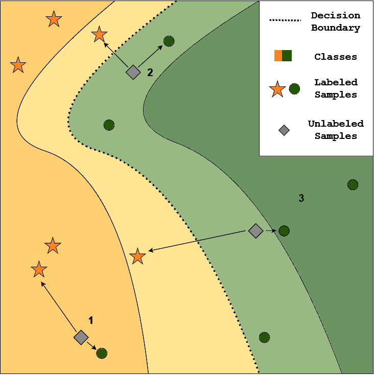
Figure 1: A conceptual example highlighting different cases how unannotated samples could be integrated into a networks feature spaces and decision boundary. Color intensity represents network prediction confidence.

The acquisition of detailed annotations for semantic segmentation is a complex and time-consuming process (Cordts et al. 2016). It becomes increasingly difficult in the medical domain due to the required expertise (Menze et al. 2014). When considering a doctor’s obligations in the clinical routine, gathering a large amount of detailed medical annotations can become almost insurmountable. Thus, these obstacles make it desirable to perform accurate semantic segmentation while minimizing the necessary annotated data.

Semi-supervised semantic segmentation solves these tasks by combining small quantities of labeled data with a lot of unannotated data for training. In recent years, several directions have been investigated such as student-teacher frameworks (Gou et al. 2021; Chen et al. 2020; Xie et al. 2020a; Pham et al. 2021), consistency regularization (Ouali, Hudelot, and Tami 2020; Sohn et al. 2020; Rebuffi et al. 2020) or pseudo-labels  (Lee et al. 2013; Iscen et al. 2019; Rizve et al. 2021). Most pseudo-label methods typically employ network predictions for unlabeled data to either save them for retraining or use them online as targets in the same iteration. They are often paired with the generation of predictions from different perturbations, e.g. data-augmentations, on an input image (Berthelot et al. 2019b, a; Sohn et al. 2020).

However, by enforcing predictions’ pre-existing biases of the network, incorrect conclusions can have a snowballing negative effect. We run into the issue of confirmation bias (Rizve et al. 2021). Yet, we argue that the positive properties of these methods can be kept, while reducing the adverse effects by taking a different path: comparing embeddings between predictions of unlabeled samples and labeled reference images to instill the supervision. For all pixels in a given unlabeled image, we find class-wise nearest-neighbors among the pixels of images in the small labeled reference set. From this, we compute a class proximities, attribute importance via confidence-based weighting and then infer the pseudo-label. By taking this detour and not directly using the class-predictions, but matching them to a known reference set, the bias towards large classes can be regulated and we bypass the problems of direct class predictions as supervision.

We illustrate the characteristics in Fig. 1. First, while the Unlabeled Pixel (UP), depicted by grey-diamond 1, would be predicted as orange, it is more similar to the misclassified green sample, and due to its proximity, we would instead pass a green pseudo-label. In the second case, we would assign a green pseudo-label to the UP2, but as its distance to both an orange and a green sample is nearly equal, the weighting would be minimal. In the third case, we assign a green pseudo-label with a high weight to the UP as it is close to a green sample and far from the second nearest class.

We view this approach as a straightforward support mechanism to pseudo-labeling in semi-supervised semantic segmentation. It is easily extended with any semi-supervised learning approaches. We demonstrate the effectiveness of our methods with extensive experiments for multi-class and binary multi-class semi-supervised semantic segmentation on the RETOUCH (Bogunović et al. 2019) and JSRT (Shiraishi et al. 2000) datasets. We achieve competitive results across these datasets, excelling especially for minimal amounts of samples. We summarize our contributions as:

1. We illustrate a different view on online pseudo-labels in semantic segmentation. By enforcing consistency between predictions and the feature space, we cover cases not handled by standard pseudo-labeling approaches.

2. We show the effectiveness of our method on different datasets and various low data settings. Thereby, we demonstrate its use for handling the challenging segmentation of overlapping labels from scarce data as we reach fully supervised performance from six labeled images.

3. We provide a detailed ablation study investigating different aspects of our pseudo-labels in various settings.

Related Work

Semi-Supervised Learning. Semi-supervised learning (SSL) utilizes few labeled samples paired with unlabeled samples to perform a given task. Recently, this field has seen significant progress (Berthelot et al. 2019b, a; Cascante-Bonilla et al. 2020; Ouali, Hudelot, and Tami 2020; Chen et al. 2020; Sohn et al. 2020; Pham et al. 2021). Most methods follow one or combinations of directions such as entropy minimization (Grandvalet, Bengio et al. 2005), consistency regularization (Tarvainen and Valpola 2017; Ji, Henriques, and Vedaldi 2019; Sohn et al. 2020) or pseudo-labeling (Lee et al. 2013; Iscen et al. 2019; Cascante-Bonilla et al. 2020). Pseudo-labeling-based approaches typically train a classifier with unlabeled data using pseudo targets derived from the model’s high-confidence predictions(Lee et al. 2013). However, pseudo-labeling can lead to noisy training due to poor calibration and as a result of incorrect high-confidence predictions (Guo et al. 2017; Rizve et al. 2021). Other methods approach pseudo-labeling by following a transductive setting, i.e. setting up a nearest-neighbor graph and perform label propagation. This generation process of pseudo-labels is not feasible in an online setting due to the high demand on run-time and memory consumption for label-propagation and is performed after a set amount of iterations  (Shi et al. 2018; Iscen et al. 2019; Liu et al. 2019). In this fashion, pseudo-labeling literature can be divided into online variants, which build pseudo-labels for unlabeled data directly during forward pass (Lee et al. 2013; Sohn et al. 2020), and offline variants, which generate new targets for the dataset in greater intervals (Iscen et al. 2019; Chen et al. 2020; Xie et al. 2020b; Cascante-Bonilla et al. 2020; Pham et al. 2021). Recently, (Taherkhani et al. 2021) matches clusters of unlabeled data to their most similar classes in an offline procedure. Taking the advantageous aspects of label-propagation methods (Shi et al. 2018; Iscen et al. 2019; Liu et al. 2019), we introduce a way to make them work online and even for semantic segmentation where pixel-wise labels add to the computational load. Favorable storage requirements of our solution make a streamlined integration with consistency regularization methods possible. In consistency regularization, predictions for varied versions of the same input are enforced to be similar. Usually this is achieved by setting up augmented versions of an input image (Sohn et al. 2020), perturbations of feature maps (Ouali, Hudelot, and Tami 2020) or different network states (Tarvainen and Valpola 2017). In our work, we intertwine online-generated pseudo-labels with consistency regularization to alleviate drawbacks in either of the two.

Semi-Supervised Segmentation. Semi-supervised semantic segmentation proposed several extensions to concepts in SSL, i.e., to consistency regularization. (French et al. 2019) integrate CutMix (Zhang et al. 2017) to enforce consistency between mixed outputs and the prediction from corresponding mixed inputs. CCT (Ouali, Hudelot, and Tami 2020) aligns the outputs of the main segmentation decoder module and auxiliary decoders trained on different perturbations to enforce consistent feature representations. PseudoSeg (Zou et al. 2021) adapts FixMatch (Sohn et al. 2020) and thus enforces consistency between segmentations of weakly and strongly augmented images employing GradCAM (Selvaraju et al. 2017). (Chen et al. 2021) use two independent networks with the same structure and enforce consistency between their predictions. In contrast to these approaches, our method utilizes labeled data in pseudo-label generation without any network alterations, rendering it flexible to integrate.

Self-Training for Medical Imaging. Network-produced supervision for unlabeled data is starting to gain traction in medical image analysis. (Tang et al. 2021) propose a self-training-based framework for mass detection in mammography leveraging medical reports. (Chaitanya et al. 2020) depict the use of contrastive self-supervised learning for semi-supervised segmentation. (Seibold et al. 2020) devise entropy minimization to localize diseases in chest radiographs while (Huo et al. 2021) propose a student-teacher framework for semi-supervised pancreas tumor segmentation.  (Reiß et al. 2021) propose to use deep supervision, which adapts networks to enforce prediction consistency between different layers of the network. However, most methods either utilize network predictions or predefined signals (Ouyang et al. 2020) as supervision. Our method is suitable for medical image analysis due to inherent structural similarities, e.g. anatomical properties make a natural fit for our method as labeled images can convey strong reference points for matching and transferring information onto unlabeled images.

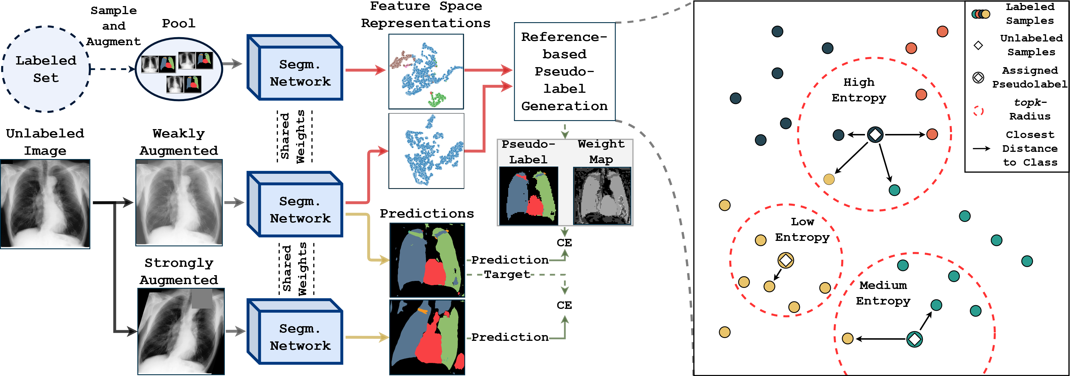
Figure 2: Overview of the proposed training step for unlabeled images. For each unlabeled image, we extract its features in addition to a pool of sampled annotated images to generate pseudo-labels. In parallel, we use the predictions of a weakly augmented sample to act as supervision for a strongly augmeted version of the image. On the right, we illustrate our reference-based pseudo-label generation process for $k=5$.

Methodology

In this section, we propose a novel strategy to generate online pseudo-labels based on label-wise feature similarities from a pool of references. We first define preliminary information, then elaborate on Reference-based Pseudo-Label Generation (RPG) and finally expand on RPG with augmentation-based consistency regularization.

Preliminaries

In the setting of semi-supervised semantic segmentation, a small set of labeled $\mathcal{S_{L}}=\{(x_{i},y_{i})\}^{N_{l}}_{i=1}$ and a large amount of unlabeled images $\mathcal{S_{U}}=\{x_{i}\}^{N_{u}}_{i=1}$ are provided. An image be defined as $x_{i}\in\mathbb{R}^{ch\times h\times w}$ with $ch$ image channels, height $h$ and width $w$. Labels be defined as $y_{i}\in\{0,\dots,c-1\}^{h\times w}$ in case of segmentation into $c$ classes or $y_{i}\in\{0,1\}^{c\times h\times w}$ if at each location more than one class can be present (multi-label segmentation). Thus, the task resolves to using $\mathcal{S_{L}}$ and $\mathcal{S_{U}}$ to find a model that correctly predicts labels on unseen images. For later purposes, we define the segmentation model as (1) a dense feature extractor $f_{\text{feat}}:\mathbb{R}^{ch\times h\times w}\rightarrow\mathbb{R}^{d\times h\times w}$ and (2) a subsequent pixel-wise classifier $f_{{cls}}:\mathbb{R}^{d\times h\times w}\rightarrow[0,1]^{c\times h\times w}$ that transforms the $d$ dimensional features at each location into class predictions. $f_{{\text{feat}}}$ is parameterized by a neural network and for $f_{{\text{cls}}}$ we leverage a $1\times 1$ convolution and normalization function (sigmoid or softmax depending on the $y_{i}$ formulation).

Reference-based Pseudolabel Generation

We propose using image-reference pairs in the pseudo-label generation process for semantic segmentation. Contrary to directly deriving pseudo-labels from network predictions, we search for a best fit in feature space among a pool of labeled reference images and transfer their semantics. We display our approach in Fig. 2.

Reference Pool. We utilize labeled references to generate pseudo-labels. Therefore, we project both labeled and un-labeled pixels into the same feature space using $f_{\text{feat}}$. Since available memory is limited, processing $h\times w$ $d$-dimensional pixel-wise representations for each image in $\mathcal{S_{L}}$ is unfeasible. Additionally, solutions like a memory-bank (Wu et al. 2018) are difficult to integrate due to sheer amount of pixel-wise representations. We approach these issues by randomly sampling a pool $\mathcal{P}$ of labeled images from $\mathcal{S_{L}}$ in each mini-batch iteration:

$$\mathcal{P}=\{(x,y)\sim\mathcal{S_{L}}\}^{p}$$ (1)

As we later generate pseudo-labels from $\mathcal{P}$, all classes have to be present otherwise the missing class-labels can not be recovered. We, thus, sample $p$ images such that each class occurs at least once in $\mathcal{P}$.

We generate our reference set $\mathcal{R}_{\mathcal{P}}$ by extracting the pixel-wise features of each image in $\mathcal{P}$ to get pairs of pixel-representations and -labels:

$$\mathcal{R}_{\mathcal{P}}=\{(f_{\text{feat}}(x),y):(x,y)\in\mathcal{P}\}.$$ (2)

To further reduce the memory constraints we sub-sample the pixel-wise representations and labels to a feasible size $s\times s$ using nearest-neighbor interpolation. In the following, we dispose of the spatial relations between pixels and only consider $\mathcal{R}_{\mathcal{P}}$ to be a set of $d$ dimensional feature vector-label pairs with $|\mathcal{R}_{\mathcal{P}}|=p\cdot h\cdot w$. By sampling $\mathcal{P}$ continuously during training, the labeled images can experience a large variation of data augmentation techniques, leading to more diverse pixel-representations in the reference set $\mathcal{R}_{\mathcal{P}}$.

Label Assignment. We build pseudo-labels by finding the closest labeled pixels in feature space from the reference pool $\mathcal{R}_{\mathcal{P}}$ for each unlabeled pixel. For each unlabeled image $u\in\mathcal{S}_{\mathcal{U}}$ in the mini-batch we extract pixel-wise features $\hat{u}=f_{\text{feat}}(u)$. We now assign the target of an unlabeled vector $\hat{u}_{\text{x},\text{y}}$ with the spatial coordinates $\text{x},\text{y}\in\mathbb{N}^{h\times w}$ based on the contextually closest feature vector in $\mathcal{R}_{\mathcal{P}}$. The clipped cosine distance $\mathcal{D}$ between of the labeled pixel-representations $r\in\mathcal{R}_{\mathcal{P}}$ and the unlabeled pixel-representations $\hat{u}_{\text{x},\text{y}}\in\hat{u}$ serves as proximity measure:

$$\mathcal{D}(r,\hat{u}_{\text{x},\text{y}})=1-\max(\frac{\sum_{i=1}^{d}r_{i}\cdot\hat{u}_{\text{x},\text{y},i}}{\sqrt{\sum_{i=1}^{d}r_{i}^{2}}\cdot\sqrt{\sum_{i=1}^{d}\hat{u}_{\text{x},\text{y},i}^{2}}+\epsilon},0),$$ (3)

with subscript $i$ indexing the $i$-th dimension of a vector and the small constant $\epsilon=1e^{-8}$. Using $\mathcal{D}$, two feature vectors have a distance of zero if they are identical and the maximum distance of one if orthogonal or contrary to each other. For each unlabeled pixel $u_{\text{x},\text{y}}$ a pseudo-label $l(u_{\text{x},\text{y}})$ is assigned based on the label of its closest sample in the reference pool:

$$l(u_{\text{x},\text{y}})=y:\mathop{\rm argmin}_{(r,y)\in\mathcal{R}_{\mathcal{P}}}\mathcal{D}(r,\hat{u}_{\text{x},\text{y}})$$ (4)

The whole image is labeled by $l(u)=\{l(u_{\text{x},\text{y}}):u_{\text{x},\text{y}}\in u\}$. Note that this way, $y$ can be either a one-hot vector or a sophisticated multi-label vector. Our approach is contrary to classical pseudo-labeling, where assigning a multi-label vector requires the network to hit manually designed thresholds for every class. Our nearest-neighbor target assignment is related to previous methods (Iscen et al. 2019; Liu et al. 2019; Mechrez, Talmi, and Zelnik-Manor 2018), however, we operate online and access multiple reference images at the same time.

Density-based Class Entropy. Overall, for an adequate pool-size $p$, this nearest-neighbor label assignments showed to be beneficial for semantic segmentation. However, we noticed a potential pitfall: For features with similar distances to several classes direct assignments mislead the network during training. To avoid this issue, we apply a weighting mechanism based on the ambiguity of an unlabeled pixel’s surroundings. With the feature $\hat{u}_{\text{x},\text{y}}$ we compute the closest distances $\delta^{j}_{\hat{u}_{\text{x},\text{y}}},j\in{1,\dots,c}$ to each class among the $k$ nearest neighbors $\mathcal{R}_{\mathcal{\mathcal{P}}}^{k}$ in feature space.

$$\delta^{j}_{\hat{u}_{\text{x},\text{y}}}=\min_{(r,y)\in\mathcal{R}_{\mathcal{P}}^{k}\land y=j}\mathcal{D}(r,\hat{u}_{\text{x},\text{y}})$$ (5)

If class $j$ is not represented in the reference pool $\mathcal{R}_{\mathcal{P}}^{k}$, it’s distance $\delta^{j}_{\hat{u}_{\text{x},\text{y}}}$ is set to one. We use these class distances to model $j$ class probabilities $\mathit{P}^{j}_{u_{\text{x},\text{y}}}$ via class-wise normalization:

$$\mathit{P}^{j}_{u_{\text{x},\text{y}}}=\frac{1-\delta^{j}_{u_{\text{x},\text{y}}}+\epsilon}{\sum_{j^{\prime}=1}^{c}1-\delta^{j^{\prime}}_{u_{\text{x},\text{y}}}+\epsilon}$$ (6)

We then calculate the weighting factor $W_{u_{\text{x},\text{y}}}$ through the normalized entropy of the class probabilities:

$$W_{u_{\text{x},\text{y}}}=1+\sum^{c}_{j=1}\mathit{P}^{j}_{u_{\text{x},\text{y}}}\frac{\log\mathit{P}^{j}_{u_{\text{x},\text{y}}}}{\log c}$$ (7)

With the factor $W_{u_{\text{x},\text{y}}}$ we put a lower weight on pseudo-labeled pixels that lie in highly ambiguous regions in the feature space. On top this weighting nudges the pseudo-labels towards including more classes instead of opting just for the most common one. This is due to the fact, that distances of all classes influence the weighting of a pixel-label-assignment. Further, this weighting handles extreme cases where e.g. $\delta^{j}_{u_{\text{x},\text{y}}}=1$ for all classes, as here the entropy will be maximal, which in turn will lead to ignoring $u_{\text{x},\text{y}}$ since $W_{u_{\text{x},\text{y}}}=0$. We illustrate further cases on the righthand side of Fig 2.

Ultimately, our method is formulated as the following loss function $\mathcal{L}_{RPG}$:

$$\mathcal{L}_{RPG}= \,\mathbb{E}_{(x,y)\in\mathcal{S}_{\mathcal{L}}}[\mathrm{CE}(f_{\text{cls}}^{c}(f_{feat}(x)),y)]$$

$$+\mathbb{E}_{x\in\mathcal{S}_{\mathcal{U}}}[\mathrm{CE}(f_{\text{cls}}^{c}(f_{feat}(x)),l(x))\cdot W_{x}],$$ (8)

with $\mathrm{CE}$ denoting binary or multi-class cross-entropy depending on the type of segmentation task.

Consistency Regularization

To showcase that our approach works complementary to consistency regularization methods in semantic segmentation, we expand the formulation of FixMatch (Sohn et al. 2020). We generate pseudo-labels from network predictions on weakly augmented images and use them as labels for strongly augmented versions of the same image, thereby enforcing consistency between them. While weak augmentations are commonly used perturbations such as random flipping, for strong augmentations, we follow RandAugment (Cubuk et al. 2020). We follow a similar setting as in Sohn  et al. (Sohn et al. 2020). Since we handle segmentation instead of classification which is done in the original work, we generate pixel-level pseudo-labels and set the designated label for the areas affected by the CutOut augmentation (DeVries and Taylor 2017) to ‘background’. For one-hot targets $y$, we use the standard pseudo-label formulation (Sohn et al. 2020)

$$l^{\prime}(u_{\text{x},\text{y}})=\begin{cases}\mathop{\rm argmax}_{c}f_{cls}^{c}(\hat{u}_{\text{x},\text{y}})&\text{, if }f_{cls}^{c}(\hat{u}_{\text{x,y}})>\tau\\ \text{ignore}&\text{, else}\end{cases}$$ (9)

and further extend the FixMatch formulation to enable multi-label segmentation as follows:

$$l^{\prime}(u_{\text{x},\text{y}})=\begin{cases}\lfloor f_{cls}^{c}(\hat{u}_{\text{x},\text{y}})\rceil&\text{, if }|f_{cls}^{c}(\hat{u}_{\text{x},\text{y}})-0.5|\\ &\quad\;\;>|0.5-\tau|\\ \text{ignore},&\text{, else}\end{cases}$$ (10)

where $\tau$ is a scalar threshold value separating labeled and ignored pixels. The whole image is labeled by choosing based on the task the respective $l^{\prime}(\cdot)$ $l^{\prime}(u)=\{l^{\prime}(u_{\text{x},\text{y}}):u_{\text{x},\text{y}}\in u\}$. We denote the final consistency regularized loss term $\mathcal{L}_{{RPG}^{+}}$ as:

$$\mathcal{L}_{{RPG}^{+}}= \mathcal{L}_{RPG}\,\,+$$ (11)

$$\mathbb{E}_{x\in\mathcal{S}_{\mathcal{U}}}[\mathrm{CE}(f_{cls}^{c}(f_{feat}(\mathit{a}_{s}(x))),\mathit{a}_{s}(l^{\prime}(x)))]$$

Methods	$N_{l}=3$	$N_{l}=6$	$N_{l}=12$	$N_{l}=24$
Baseline	$0.59\pm 0.04$	$0.73\pm 0.02$	$0.81\pm 0.01$	$0.85\pm 0.01$
Pseudolabelτ=0.8 (Lee et al. 2013)	$0.56\pm 0.04$	$0.73\pm 0.04$	$0.81\pm 0.03$	$0.87\pm 0.01$
Pseudolabelτ=0.95 (Lee et al. 2013)	$0.57\pm 0.03$	$0.74\pm 0.03$	$0.82\pm 0.02$	$0.87\pm 0.01$
Nearest Neighbor	$0.64\pm 0.05$	$0.76\pm 0.02$	$0.81\pm 0.02$	$0.84\pm 0.01$
FixMatchτ=0.8 (Sohn et al. 2020)	$0.71\pm 0.05$	$0.79\pm 0.02$	$0.80\pm 0.01$	$0.85\pm 0.00^{*}$
FixMatchτ=0.95 (Sohn et al. 2020)	$0.67\pm 0.05$	$0.77\pm 0.02$	$0.81\pm 0.02$	$0.85\pm 0.01^{*}$
RPG (Ours)	$0.71\pm 0.02$	$0.79\pm 0.02$	$0.83\pm 0.02$	$0.87\pm 0.01$
RPG+ (Ours)	$\mathbf{0.77\pm 0.05^{*}}$	$\mathbf{0.85\pm 0.01^{*}}$	$\mathbf{0.87\pm 0.00^{*}}$	$\mathbf{0.88\pm 0.01^{*}}$
Full Access ($N_{l}=123$)	0.85

Table 1: Performance comparison of our work to related work on the datasets JSRT. ^∗ denotes that due to lacking convergence the model was trained twice the iterations. Bold and underlines denote best and second best performance.

Experiments

Experimental Setup

Datasets. We evaluate our method on two medical tasks, namely chest radiograph anatomy segmentation and retinal fluid segmentation. For multi-label anatomy segmentation, we employ the public JSRT-dataset (Shiraishi et al. 2000). It consists of five potentially pixel-wise overlapping classes (right/left clavicle, right/left lung, heart). The dataset officially exists with two sets of images (123/124). For each amount of labeled images, we choose to generate five distinct random splits from the first set using $N_{l}$ labeled images ($N_{l}\in{3,6,12,24}$). For each split, we use five images of the first set for validation while using the second set for testing.

To further display the effect of our proposed method for overlapping labels in small data setting, we expand upon the JSRT dataset by using more fine-grained annotations for a total of 72 labels belonging to the supercategories of heart, lung, ribs, spine, and others. As a result, each label consists of fewer annotated pixels than the large labels in JSRT, i.e., the lung consists of its five lobes compared to two lung halves. For this task, a medical expert annotated two chest radiographs taking up to 3 hours per image. We evaluate the performance on this task by fusing our fine-grained classes into the corresponding JSRT labels , e.g. right upper, middle and lower lung lobe correspond to the right lung. We use five JSRT labeled images of the first set as validation and test the performance on the second set of JSRT. We further elaborate on the annotations in the supplementary.

For multi-class retinal fluid segmentation, we utilize the Spectralis vendor of the RETOUCH data set consisting of 14 optical coherence tomography volumes with 49 b-scans each. We follow the setup of (Reiß et al. 2021) and thus perform 10-fold cross-validation with training sets using $N_{l}$ labeled images ($N_{l}\in{3,6,12,24}$), with validation and test sets of roughly equal size on Spectralis, and ensure that in each split, all diseases show at least once in the mask labels.

We use mean Intersection over Union (mIoU) as the performance metric. We evaluate our method every tenth epoch, apply the best-performing model on the validation set to the test set, and report the mean and standard deviation.

Implementation Details. For our segmentation model we use the common UNet architecture (Ronneberger, Fischer, and Brox 2015) with batchnorm (Ioffe and Szegedy 2015) and bilinear up-scaling blocks. The function $f_{\text{feat}}$ which is used for feature extraction describes the network up to the penultimate layer. The function $f_{\text{cls}}$ is a $1\times 1$ convolution followed by a sigmoid function for JSRT and Softmax for RETOUCH. We initialize the network using standard Xavier initialization (Glorot and Bengio 2010). We optimize using Adam (Kingma and Ba 2014) with learning rate and weight decay of $0.0005$ for 100 epochs on JSRT, 200 on extended JSRT and 50 epochs on RETOUCH respectively. As data augmentations, we use random cropping, rotation, additive noise, and color jitters with additional random flipping. For JSRT, we use batch size $5$ with image size 512, while for RETOUCH we use batch size $8$ following the preprocessing utilized in (Reiß et al. 2021). For all experiments, we build each batch as a combination of $\mathcal{P}$ with $p=3$ and randomly sampled images of the whole dataset. We set the number of considered nearest neighbors $k=7000$ and the representation map size $s=64$. All experiments were run on one 11GB NVIDIA GeForce RTX 2080.

$p$	$N_{l}=3$	$N_{l}=6$	$N_{l}=12$	$N_{l}=24$
1	$0.52\pm 0.02$	$0.66\pm 0.04$	$0.74\pm 0.02$	$0.78\pm 0.01$
2	$0.58\pm 0.04$	$0.72\pm 0.03$	$0.77\pm 0.03$	$0.82\pm 0.01$
3	$0.64\pm 0.05$	$0.76\pm 0.02$	$0.81\pm 0.02$	$0.84\pm 0.01$
4	$0.65\pm 0.04$	$0.76\pm 0.02$	$0.79\pm 0.03$	$0.84\pm 0.01$
5	$0.66\pm 0.03$	$0.77\pm 0.02$	$0.82\pm 0.02$	$0.84\pm 0.01$

Table 2: Comparison of Nearest-Neighbor performance for different memory bank sizes.

$p$	$k=25\%$	$k=50\%$	$k=75\%$	$k=100\%$
1	$0.55\pm 0.03$	$0.57\pm 0.02$	$0.56\pm 0.01$	$0.52\pm 0.04$
2	$0.60\pm 0.04$	$0.62\pm 0.03$	$0.58\pm 0.03$	$0.51\pm 0.04$
3	$0.66\pm 0.03$	$0.70\pm 0.02$	$0.67\pm 0.02$	$0.52\pm 0.06$
4	$0.68\pm 0.03$	$0.68\pm 0.03$	OOM	OOM
5	$0.68\pm 0.02$	OOM	OOM	OOM

Table 3: Comparison of RPG for different $k$ and image pool sizes. ’OOM’ denotes ’Out Of Memory’.

Methods	Data	Right Lung	Left Lung	Heart	Right Clavicle	Left Clavicle	Mean
Baseline	JSRT $N_{l}=3$	$0.83\pm 0.02$	$0.81\pm 0.01$	$0.59\pm 0.02$	$0.47\pm 0.05$	$0.42\pm 0.07$	$0.59\pm 0.04$
Pseudolabelτ=0.8		$0.86\pm 0.02$	$0.87\pm 0.02$	$0.65\pm 0.10$	$0.35\pm 0.06$	$0.28\pm 0.06$	$0.56\pm 0.04$
FixMatchτ=0.8		$0.94\pm 0.00$	$0.93\pm 0.00$	$0.82\pm 0.03$	$0.50\pm 0.09$	$0.44\pm 0.14$	$0.71\pm 0.05$
RPG (Ours)		$0.91\pm 0.01$	$0.90\pm 0.01$	$0.71\pm 0.02$	$0.55\pm 0.04$	$\mathbf{0.55\pm 0.03}$	$0.71\pm 0.02$
RPG+∗ (Ours)		$\mathbf{0.95\pm 0.00}$	$\mathbf{0.95\pm 0.00}$	$\mathbf{0.85\pm 0.02}$	$\mathbf{0.60\pm 0.09}$	$0.50\pm 0.15$	$\mathbf{0.77\pm 0.05}$
Baseline	Custom $N_{l}=2$	0.1105	0.0994	0.2335	0.0526	0.0256	0.1043
Pseudolabelτ=0.8		0.2335	0.0847	0.0920	0.0000	0.0000	0.0820
FixMatchτ=0.8		0.0504	0.0463	0.0041	0.0000	0.0000	0.0246
RPG (Ours)		0.6065	0.4592	0.5108	0.0000	0.0000	0.3153
RPG+ (Ours)		0.6326	0.4852	0.5636	0.0671	0.0168	0.3531

Table 4: Performance comparison on JSRT and our extended annotations (Custom). ^∗ denotes a training of twice the iterations. Bold and underlined denote best and second best performance respectively.

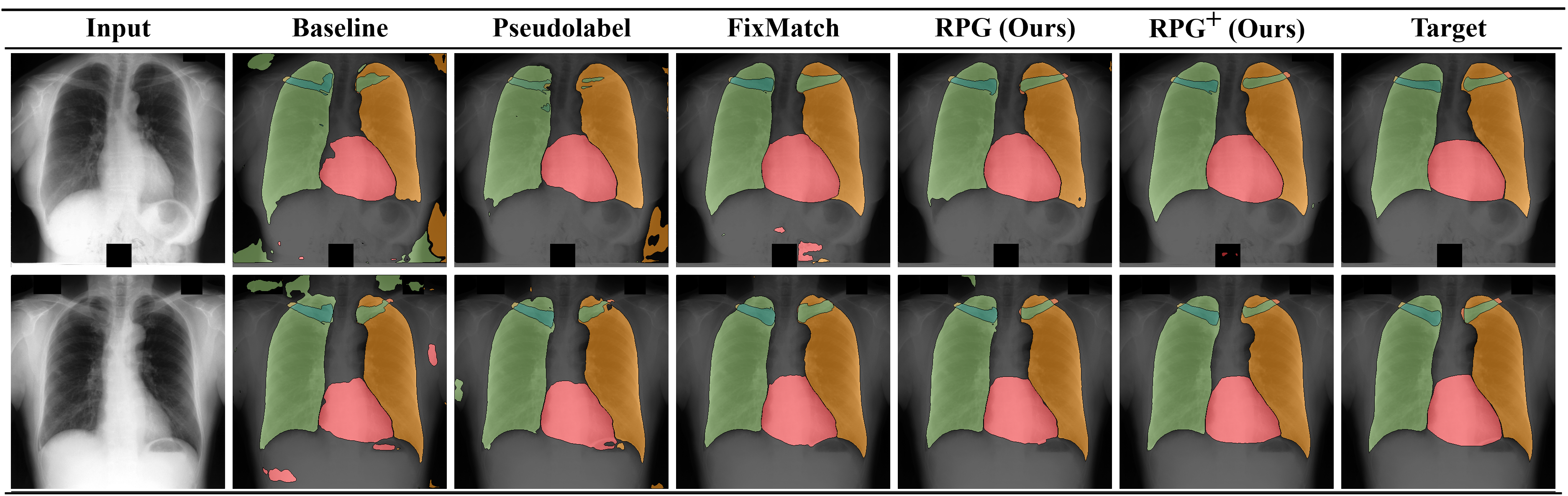
Figure 3: Qualitative Segmentation Results on the JSRT (Shiraishi et al. 2000) dataset for $N_{l}=6$.

Baselines and Methods. First, we employ a standard UNet Baseline using only the available annotated data as supervision. Due to the low amount of seen images, we run these models for the same amount of iterations instead of the same amount of epochs. Next, we take a look at the original Pseudolabel method proposed by (Lee et al. 2013), which we test for different thresholds $\tau$. Further, we compare a naive Nearest Neighbor label assignment without a weighting function. We also compare against recent methods of MLDS (Reiß et al. 2021), which uses deep supervision paired with a Mean-Teacher (Tarvainen and Valpola 2017) setup, and FixMatch (Sohn et al. 2020) utilizing strongly and weakly augmented prediction comparisons.

Ablation Studies

Pool Size for Pseudo-Label Assignment. To show the potential of nearest-neighbor-based pseudo-label generation for semantic segmentation, we investigate the segmentation performance for different combinations of pool size and the amount of annotated images. Table 2 shows that if only a single image is considered the segmentation ability of the network is rather poor but as we increase the number of images in the pool, we see a steady performance increase across all amounts of annotated images. We note that while increasing the pool size overall also positively affects performance, the improvement past $p=3$ is substantially less while the needed memory rises at a constant rate. Thus, we see $p=3$ as a good trade-off between performance and memory consumption and maintain it for all further experiments.

Amount of Observed Neighbors. We expand upon the nearest neighbor assignment in RPG with our weighting scheme. Therefore, we investigate the impact of the effective radius in feature space on our density-based class entropy weighting for different pool sizes $p$ and relative amounts of considered neighbors $k$ for $N_{l}=3$. We display the results in Table 3 with each column representing the relative amount of all considered features in the reference pool $\mathcal{R}_{\mathcal{P}}$. Independently of the pool size, we see that increasing $k$ improves over just the nearest-neighbor assignments shown in the first column of Table 2. The performance increases up until $50\%$ of all existing features where it peaks and falls off drastically for larger $k$’s. This indicates that an increased search radius is helpful but finding the optimal $k$ is difficult. Due to memory constraints we did not test larger $k$’s for bigger pool sizes.

Methods	$N_{l}=3$	$N_{l}=6$	$N_{l}=12$	$N_{l}=24$
Baseline	$0.15\pm 0.07$	$0.27\pm 0.08$	$0.35\pm 0.06$	$0.49\pm 0.05$
IIC (Ji, Henriques, and Vedaldi 2019)	$0.22\pm 0.09$	$0.32\pm 0.07$	$0.41\pm 0.07$	$0.53\pm 0.06$
Perone and Cohen-Adad (2018)	$0.21\pm 0.09$	$0.31\pm 0.10$	$0.39\pm 0.07$	$0.50\pm 0.08$
MLDS (Reiß et al. 2021)	$0.16\pm 0.15$	$0.35\pm 0.11$	$0.54\pm 0.09$	$\mathbf{0.59\pm 0.07}$
RPG (Ours)	$0.21\pm 0.10$	$0.30\pm 0.08$	$0.45\pm 0.08$	$0.54\pm 0.08$
RPG+ (Ours)	$\mathbf{0.31\pm 0.11}$	$\mathbf{0.45\pm 0.10}$	$\mathbf{0.55\pm 0.08}$	$\mathbf{0.59\pm 0.08}$
Full Access ($N_{l}=415$)	$0.62\pm 0.05$

Table 5: Performance comparison on Retouch. Bold and underlined denote best and second best performance respectively.

Quantitative Results

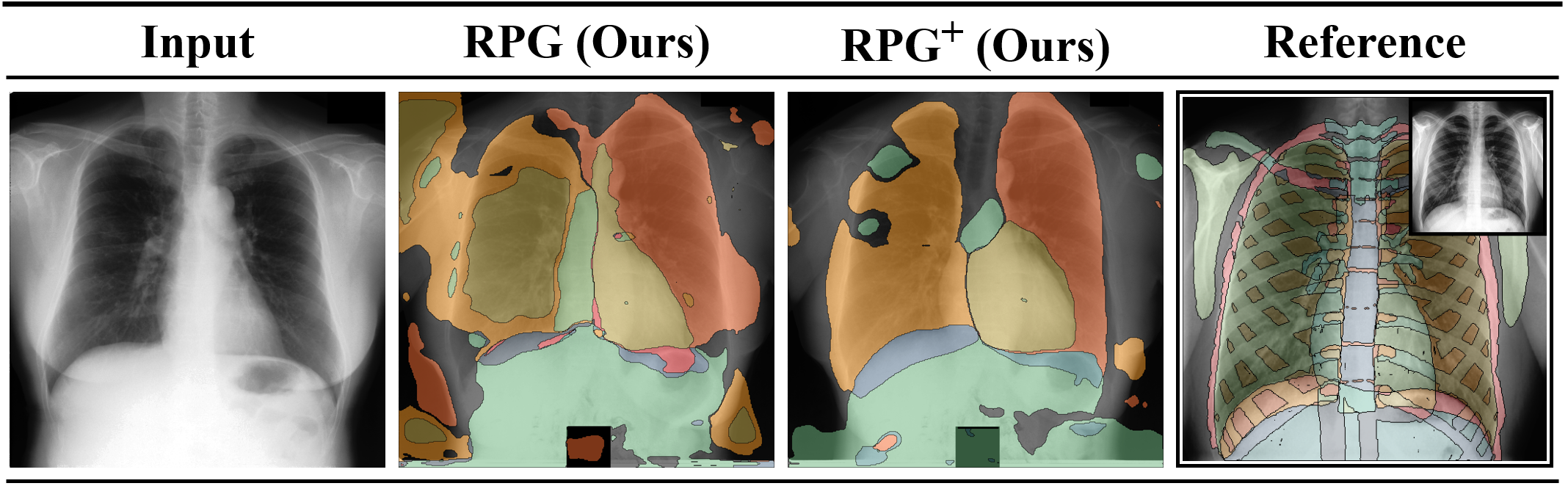
Figure 4: Qualitative Segmentation Results on extended anatomical x-ray annotations.

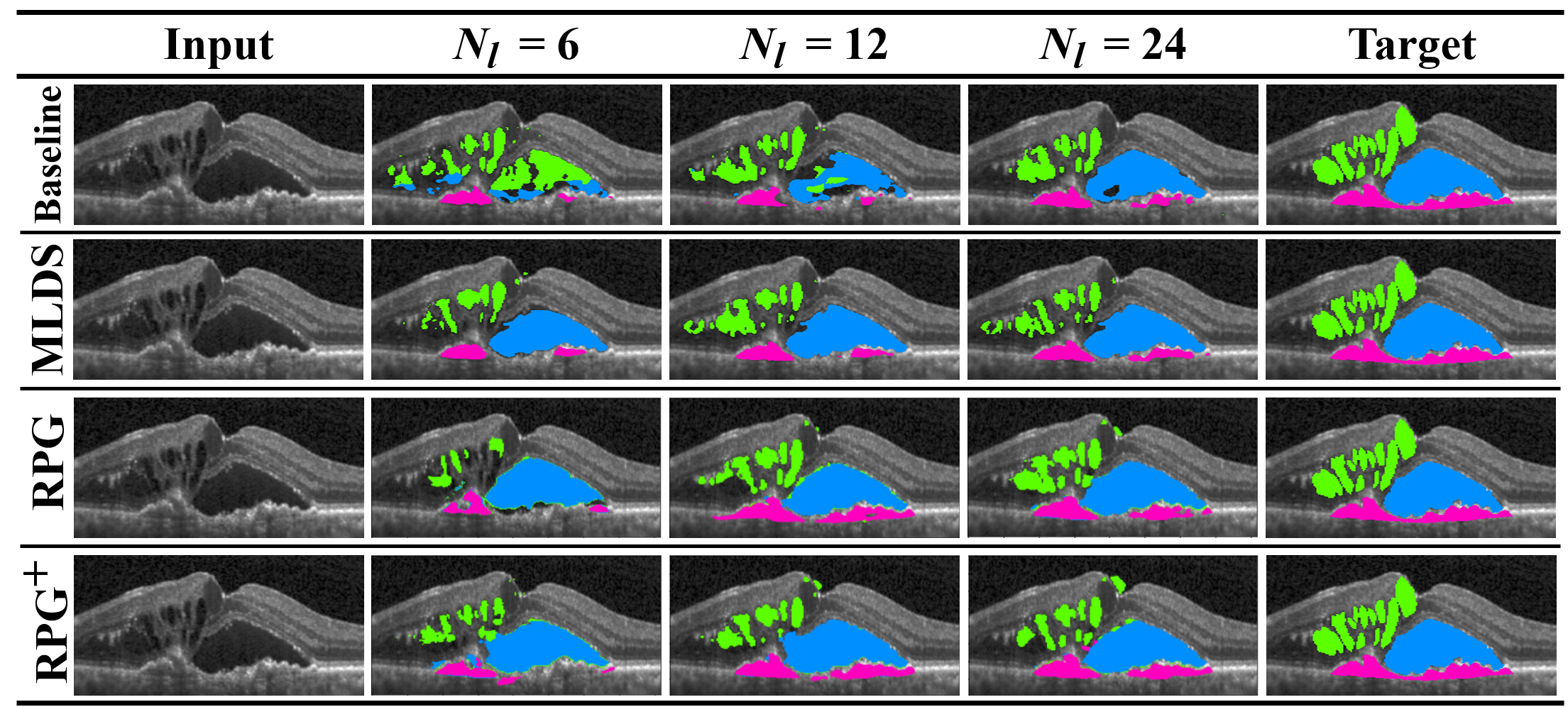
Figure 5: Qualitative Results on RETOUCH.

Results on JSRT. In Table 1, we display the mIoU of various methods for multi-label anatomy segmentation. Standard pseudo-labeling shows varying performance depending on the chosen threshold, and while it performs well for more annotated images, the performance even falls below the baseline in the low data case for any chosen threshold. Nearest Neighbor pseudo-labels improve over the baseline for few samples by $3$-$5\%$ but show slightly worse results for 24 annotated examples. FixMatch gains $12\%$ above the baseline for $N_{l}=3$, but it struggles for more annotations despite taking longer to converge. Both FixMatch and standard Pseudolabeling show varying performance for different $\tau$. Our proposed $RPG$ performs equally to FixMatch for smaller $N_{l}$ and outperforms it for larger $N_{l}$s while not using strong augmentations. We further see that the integration of strongly augmented images in $RPG^{+}$ improves the performance of $RPG$ for all settings gaining $18\%$ over the baseline for $N_{l}=3$ and matches fully supervised performance with six labeled samples.

We further demonstrate the class-wise performance for three annotated samples on the top of Table 4. We see that the baseline as well as pseudo labeling struggle with less common classes like the clavicles. FixMatch shows considerable improvements for the classes with more annotated pixels, while the performance for the clavicles only slightly improves. $RPG$ also improves over the baseline for heart and lungs, but shows significant improvements for the difficult clavicles. Furthermore, $RPG^{+}$ combines the aspects of $RPG$ and augmentation-based consistency regularization, which noticeably improves all categories apart from the right clavicle with gains up to absolute $26\%$ over the baseline. We display segmentation predictions in Fig. 3, where class-wise shortcomings of the different methods become visible.

Results on Extended JSRT. In the bottom half of Table 4, we display the results when using our fine-grained annotations of JSRT. The baseline of training simply on the annotated images achieves $10.43\%$ mIoU. Both prediction-based pseudolabeling methods struggle in this complex low data environment and perform worse than the baseline. In contrast, RPG manages to correctly predict classes of the super-categories Left Lung, Right Lung and Heart leading to a mIoU of $31.53\%$ thus improving upon the baseline by absolute $21.10\%$. RPG⁺ slightly boosts this further to a mIoU of $35.31\%$. We display the extended anatomy segmentations in Fig. 4. We see RPG⁺ managing to reconstruct the lung-subcategories, ventricles of the heart and the sub-diaphragm, but struggling with explicit predictions of bone structures.

Results on Spectralis. We display our results for the Spectralis dataset in Table 5. Here, we also see $RPG$ outperforming the baseline for all considered $N_{l}$, thus showing its usability for the multi-class segmentation setting. $RPG^{+}$ noticeably outperforms other methods especially for the low data schemes of $N_{l}=3$ and $N_{l}=6$ by up to 15% while having the same performance as MLDS for $N_{l}=24$. We display qualitative comparisons in Fig. 5.

Conclusion

In this work, we proposed a novel way of generating supervision for segmentation. We use labeled images as reference material, match pixels in an unlabeled image to their semantic counterparts, and allocate the corresponding label seen in the reference. This way, we do not fall into pitfalls common with prediction-based pseudo-labeling such as confirmation bias. Since no additional networks or alterations to a given architecture are necessary, our proposed method can easily be plugged into any existing framework. We argue that this way of pseudo-label generation is especially fitting for medical image analysis due structural similarity provided by underlying anatomical structures. We demonstrate the effectiveness of our approach through extensive experiments on chest X-ray anatomy segmentation and retinal fluid segmentation. We achieve fully supervised performance with only a handful of samples, thus, cutting the annotation cost by 95%. Our code and additional information are available in the supplementary.

References

- Berthelot et al. (2019a) Berthelot, D.; Carlini, N.; Cubuk, E. D.; Kurakin, A.; Sohn, K.; Zhang, H.; and Raffel, C. 2019a. Remixmatch: Semi-supervised learning with distribution alignment and augmentation anchoring. arXiv preprint arXiv:1911.09785.
- Berthelot et al. (2019b) Berthelot, D.; Carlini, N.; Goodfellow, I.; Papernot, N.; Oliver, A.; and Raffel, C. 2019b. Mixmatch: A holistic approach to semi-supervised learning. arXiv preprint arXiv:1905.02249.
- Bogunović et al. (2019) Bogunović, H.; et al. 2019. RETOUCH: The Retinal OCT Fluid Detection and Segmentation Benchmark and Challenge. IEEE Transactions on Medical Imaging, 38(8): 1858–1874.
- Cascante-Bonilla et al. (2020) Cascante-Bonilla, P.; Tan, F.; Qi, Y.; and Ordonez, V. 2020. Curriculum labeling: Self-paced pseudo-labeling for semi-supervised learning. arXiv e-prints, arXiv–2001.
- Chaitanya et al. (2020) Chaitanya, K.; Erdil, E.; Karani, N.; and Konukoglu, E. 2020. Contrastive learning of global and local features for medical image segmentation with limited annotations. In Larochelle, H.; Ranzato, M.; Hadsell, R.; Balcan, M. F.; and Lin, H., eds., Advances in Neural Information Processing Systems, volume 33, 12546–12558. Curran Associates, Inc.
- Chen et al. (2020) Chen, T.; Kornblith, S.; Swersky, K.; Norouzi, M.; and Hinton, G. 2020. Big self-supervised models are strong semi-supervised learners. arXiv preprint arXiv:2006.10029.
- Chen et al. (2021) Chen, X.; Yuan, Y.; Zeng, G.; and Wang, J. 2021. Semi-Supervised Semantic Segmentation with Cross Pseudo Supervision. In Proceedings of the IEEE/CVF Conference on Computer Vision and Pattern Recognition, 2613–2622.
- Cordts et al. (2016) Cordts, M.; et al. 2016. The cityscapes dataset for semantic urban scene understanding. In Proceedings of the IEEE conference on computer vision and pattern recognition, 3213–3223.
- Cubuk et al. (2020) Cubuk, E. D.; Zoph, B.; Shlens, J.; and Le, Q. V. 2020. Randaugment: Practical automated data augmentation with a reduced search space. In Proceedings of the IEEE/CVF Conference on Computer Vision and Pattern Recognition Workshops, 702–703.
- DeVries and Taylor (2017) DeVries, T.; and Taylor, G. W. 2017. Improved regularization of convolutional neural networks with cutout. arXiv preprint arXiv:1708.04552.
- French et al. (2019) French, G.; Aila, T.; Laine, S.; Mackiewicz, M.; and Finlayson, G. 2019. Consistency regularization and cutmix for semi-supervised semantic segmentation. arXiv preprint arXiv:1906.01916, 2(4): 5.
- Glorot and Bengio (2010) Glorot, X.; and Bengio, Y. 2010. Understanding the difficulty of training deep feedforward neural networks. In Proceedings of the thirteenth international conference on artificial intelligence and statistics, 249–256. JMLR Workshop and Conference Proceedings.
- Gou et al. (2021) Gou, J.; Yu, B.; Maybank, S. J.; and Tao, D. 2021. Knowledge distillation: A survey. International Journal of Computer Vision, 129(6): 1789–1819.
- Grandvalet, Bengio et al. (2005) Grandvalet, Y.; Bengio, Y.; et al. 2005. Semi-supervised learning by entropy minimization. In CAP, 281–296.
- Guo et al. (2017) Guo, C.; Pleiss, G.; Sun, Y.; and Weinberger, K. Q. 2017. On calibration of modern neural networks. In International Conference on Machine Learning, 1321–1330. PMLR.
- Huo et al. (2021) Huo, X.; et al. 2021. ATSO: Asynchronous Teacher-Student Optimization for Semi-Supervised Image Segmentation. In Proceedings of the IEEE/CVF Conference on Computer Vision and Pattern Recognition, 1235–1244.
- Ioffe and Szegedy (2015) Ioffe, S.; and Szegedy, C. 2015. Batch normalization: Accelerating deep network training by reducing internal covariate shift. In International conference on machine learning, 448–456. PMLR.
- Iscen et al. (2019) Iscen, A.; Tolias, G.; Avrithis, Y.; and Chum, O. 2019. Label propagation for deep semi-supervised learning. In Proceedings of the IEEE/CVF Conference on Computer Vision and Pattern Recognition, 5070–5079.
- Ji, Henriques, and Vedaldi (2019) Ji, X.; Henriques, J. F.; and Vedaldi, A. 2019. Invariant information clustering for unsupervised image classification and segmentation. In Proceedings of the IEEE/CVF International Conference on Computer Vision, 9865–9874.
- Kingma and Ba (2014) Kingma, D. P.; and Ba, J. 2014. Adam: A method for stochastic optimization. arXiv preprint arXiv:1412.6980.
- Lee et al. (2013) Lee, D.-H.; et al. 2013. Pseudo-label: The simple and efficient semi-supervised learning method for deep neural networks. In Workshop on challenges in representation learning, ICML, volume 3.
- Liu et al. (2019) Liu, B.; Wu, Z.; Hu, H.; and Lin, S. 2019. Deep metric transfer for label propagation with limited annotated data. In Proceedings of the IEEE/CVF International Conference on Computer Vision Workshops, 0–0.
- Mechrez, Talmi, and Zelnik-Manor (2018) Mechrez, R.; Talmi, I.; and Zelnik-Manor, L. 2018. The contextual loss for image transformation with non-aligned data. In Proceedings of the European conference on computer vision (ECCV), 768–783.
- Menze et al. (2014) Menze, B. H.; et al. 2014. The multimodal brain tumor image segmentation benchmark (BRATS). IEEE transactions on medical imaging, 34(10): 1993–2024.
- Ouali, Hudelot, and Tami (2020) Ouali, Y.; Hudelot, C.; and Tami, M. 2020. Semi-supervised semantic segmentation with cross-consistency training. In Proceedings of the IEEE/CVF Conference on Computer Vision and Pattern Recognition, 12674–12684.
- Ouyang et al. (2020) Ouyang, C.; Biffi, C.; Chen, C.; Kart, T.; Qiu, H.; and Rueckert, D. 2020. Self-supervision with superpixels: Training few-shot medical image segmentation without annotation. In European Conference on Computer Vision, 762–780. Springer.
- Pham et al. (2021) Pham, H.; Dai, Z.; Xie, Q.; and Le, Q. V. 2021. Meta pseudo labels. In Proceedings of the IEEE/CVF Conference on Computer Vision and Pattern Recognition, 11557–11568.
- Rebuffi et al. (2020) Rebuffi, S.-A.; Ehrhardt, S.; Han, K.; Vedaldi, A.; and Zisserman, A. 2020. Semi-supervised learning with scarce annotations. In Proceedings of the IEEE/CVF Conference on Computer Vision and Pattern Recognition Workshops, 762–763.
- Reiß et al. (2021) Reiß, S.; Seibold, C.; Freytag, A.; Rodner, E.; and Stiefelhagen, R. 2021. Every annotation counts: Multi-label deep supervision for medical image segmentation. In Proceedings of the IEEE/CVF Conference on Computer Vision and Pattern Recognition, 9532–9542.
- Rizve et al. (2021) Rizve, M. N.; Duarte, K.; Rawat, Y. S.; and Shah, M. 2021. In defense of pseudo-labeling: An uncertainty-aware pseudo-label selection framework for semi-supervised learning. arXiv preprint arXiv:2101.06329.
- Ronneberger, Fischer, and Brox (2015) Ronneberger, O.; Fischer, P.; and Brox, T. 2015. U-net: Convolutional networks for biomedical image segmentation. In International Conference on Medical image computing and computer-assisted intervention, 234–241. Springer.
- Seibold et al. (2020) Seibold, C.; Kleesiek, J.; Schlemmer, H.-P.; and Stiefelhagen, R. 2020. Self-Guided Multiple Instance Learning for Weakly Supervised Thoracic DiseaseClassification and Localizationin Chest Radiographs. In Proceedings of the Asian Conference on Computer Vision (ACCV).
- Selvaraju et al. (2017) Selvaraju, R. R.; Cogswell, M.; Das, A.; Vedantam, R.; Parikh, D.; and Batra, D. 2017. Grad-cam: Visual explanations from deep networks via gradient-based localization. In Proceedings of the IEEE international conference on computer vision, 618–626.
- Shi et al. (2018) Shi, W.; Gong, Y.; Ding, C.; Tao, Z. M.; and Zheng, N. 2018. Transductive semi-supervised deep learning using min-max features. In Proceedings of the European Conference on Computer Vision (ECCV), 299–315.
- Shiraishi et al. (2000) Shiraishi, J.; et al. 2000. Development of a digital image database for chest radiographs with and without a lung nodule: receiver operating characteristic analysis of radiologists’ detection of pulmonary nodules. American Journal of Roentgenology, 174(1): 71–74.
- Sohn et al. (2020) Sohn, K.; Berthelot, D.; Li, C.-L.; Zhang, Z.; Carlini, N.; Cubuk, E. D.; Kurakin, A.; Zhang, H.; and Raffel, C. 2020. Fixmatch: Simplifying semi-supervised learning with consistency and confidence. arXiv preprint arXiv:2001.07685.
- Taherkhani et al. (2021) Taherkhani, F.; Dabouei, A.; Soleymani, S.; Dawson, J.; and Nasrabadi, N. M. 2021. Self-Supervised Wasserstein Pseudo-Labeling for Semi-Supervised Image Classification. In Proceedings of the IEEE/CVF Conference on Computer Vision and Pattern Recognition, 12267–12277.
- Tang et al. (2021) Tang, Y.; et al. 2021. Leveraging Large-Scale Weakly Labeled Data for Semi-Supervised Mass Detection in Mammograms. In Proceedings of the IEEE/CVF Conference on Computer Vision and Pattern Recognition, 3855–3864.
- Tarvainen and Valpola (2017) Tarvainen, A.; and Valpola, H. 2017. Mean teachers are better role models: Weight-averaged consistency targets improve semi-supervised deep learning results. arXiv preprint arXiv:1703.01780.
- Wu et al. (2018) Wu, Z.; Xiong, Y.; Yu, S. X.; and Lin, D. 2018. Unsupervised feature learning via non-parametric instance discrimination. In Proceedings of the IEEE conference on computer vision and pattern recognition, 3733–3742.
- Xie et al. (2020a) Xie, Q.; Luong, M.-T.; Hovy, E.; and Le, Q. V. 2020a. Self-Training With Noisy Student Improves ImageNet Classification. In Proceedings of the IEEE/CVF Conference on Computer Vision and Pattern Recognition (CVPR).
- Xie et al. (2020b) Xie, Q.; Luong, M.-T.; Hovy, E.; and Le, Q. V. 2020b. Self-training with noisy student improves imagenet classification. In Proceedings of the IEEE/CVF Conference on Computer Vision and Pattern Recognition, 10687–10698.
- Zhang et al. (2017) Zhang, H.; Cisse, M.; Dauphin, Y. N.; and Lopez-Paz, D. 2017. mixup: Beyond empirical risk minimization. arXiv preprint arXiv:1710.09412.
- Zou et al. (2021) Zou, Y.; Zhang, Z.; Zhang, H.; Li, C.-L.; Bian, X.; Huang, J.-B.; and Pfister, T. 2021. PseudoSeg: Designing Pseudo Labels for Semantic Segmentation. In International Conference on Learning Representations.