Projection methods for Neural Field equations

Abstract

Neural field models are nonlinear integro-differential equations for the evolution of neuronal activity, and they are a prototypical large-scale, coarse-grained neuronal model in continuum cortices. Neural fields are often simulated heuristically and, in spite of their popularity in mathematical neuroscience, their numerical analysis is not yet fully established. We introduce generic projection methods for neural fields, and derive a-priori error bounds for these schemes. We extend an existing framework for stationary integral equations to the time-dependent case, which is relevant for neuroscience applications. We find that the convergence rate of a projection scheme for a neural field is determined to a great extent by the convergence rate of the projection operator. This abstract analysis, which unifies the treatment of collocation and Galerkin schemes, is carried out in operator form, without resorting to quadrature rules for the integral term, which are introduced only at a later stage, and whose choice is enslaved by the choice of the projector. Using an elementary timestepper as an example, we demonstrate that the error in a time stepper has two separate contributions: one from the projector, and one from the time discretisation. We give examples of concrete projection methods: two collocation schemes (piecewise-linear and spectral collocation) and two Galerkin schemes (finite elements and spectral Galerkin); for each of them we derive error bounds from the general theory, introduce several discrete variants, provide implementation details, and present reproducible convergence tests.

1 Introduction

Neural field models are integro-differential equations describing the spatially-extended, coarse-grained activity of neurons in continuum cortices. The simplest and most studied neural field model is written as

(1) $$\partial_{t}u(x,t)=-u(x,t)+\int_{\Omega}w(x,y)f(u(y,t))\,dy+\xi(x,t),\qquad (x,t)\in\Omega\times J$$

$$u(x,t_{0})=u_{0}, x\in\Omega.$$

where $u(x,t)$ is the voltage of a neuronal population at time $t$ and point $x$ in the cortex $\Omega$, which is a compact domain in $\mathbb{R}^{d}$. The function $w(x,y)$ is the synaptic kernel, modelling synaptic strengths from point $y$ to point $x$ in the tissue, whereas $f$ is the firing rate of the population; the function $\xi$ models an external input. Finally, $J$ is a time interval containing $t_{0}$, typically $J=[t_{0},t_{0}+T]$ or $J=[t_{0}-T,t_{0}+T]$. Intuitively, the first term in the right-hand side of the evolution equation in Eq. 1 models local decay, while the integral term collects inputs from the whole cortex. Typically the function $f$ is taken to be a steep, bounded sigmoidal function (approximating a Heaviside step function), hence a neuronal patch in $y$ contributes to the activity in $x$ nonlinearly, and only if its voltage is sufficiently high.

Since their introduction by Wilson and Cowan [55], and Amari [2], neural fields have been used to analyse and reproduce macroscopic cortical patters of activity, including localised stationary bumps, travelling waves and spiral waves. As discussed in several mathematical neuroscience reviews and textbooks [20, 21, 16, 14, 19], the model Eq. 1 can be extended in many ways, including multiple neuronal populations, stochastic forcing, and distributed delays.

Neural field equations support a wide variety of healthy and pathological neuronal patterns; these relatively simple models are a popular choice for studying macroscopic neural activity, and they display a dynamical repertoire observable in more detailed, realistic cortical models [16, 14, 19]. The study of neural fields as dynamical systems is now well established, and the literature contains mostly heuristic numerical simulations of these models (in addition to the textbooks [21, 14, 19] and references therein, see also [26, 29, 27, 47, 32, 36, 54, 48]) and empirical convergence studies of selected numerical schemes [47, 42].

By contrast, the numerical analysis of neural fields is much less developed. Intuitively, a numerical scheme can be derived by picking a spatial grid, approximating the integral with a quadrature scheme, and using a time-stepper for the corresponding set of ODEs. Convergence results are limited to these schemes (which we will classify later as discrete collocation schemes) in deterministic neural fields [39], neural fields with anisotropic diffusion [11], stochastic neural fields [38, 33], and neural fields with distributed delays [25, 44].

The present paper aims to provide an abstract framework for the development of numerical schemes for neural field equations, thereby laying the foundations for a systematic treatment of these models. Such theoretical developments are important: (i) Numerical implementations of neural field models are becoming available in dedicated software [37, 43, 9], yet a generic numerical analytical characterisation of the schemes employed in simulations is still missing. (ii) The Cauchy problem Eq. 1 is the archetype of models for cortical activity, being spatially extended, nonlocal and nonlinear; hence, these equations are useful to prototype numerical schemes for the neurosciences. (iii) It is hoped that a rigorous numerical analysis of neural fields will help devising schemes for large scale models, overcoming the expensive function evaluations which they currently require, owing to the nonlocal term.

Our approach is to define an abstract function space setup for the numerical treatment of Eq. 1, and study schemes in operator form. The strategy pursued in this article is to avoid the discretisation of the neural field problem until the very last step. This is a useful guiding principle in modern numerical analysis, as it allows to understand properties of the scheme in great generality, prior to the spatial discretisation step.

We characterise schemes for neural fields in terms of a projector $P_{n}$ from the ambient Banach space $\mathbb{X}$ on which Eq. 1 is posed, to a finite-dimensional approximating subspace $\mathbb{X}_{n}$. We show that the choice of $\mathbb{X}$, $\mathbb{X}_{n}$, and $P_{n}$ dictates the nature of the employed scheme and its convergence properties: roughly speaking, projection schemes for Eq. 1 converge at the same speed as a projection $P_{n}v$ converges to $v$ in $\mathbb{X}$.

This approach has been used before for integral equations, but not for neural fields. Steady states of Eq. 1 satisfy a Hammerstein equation, for which projection schemes have been studied rigorously in research articles by several authors [4, 8, 35, 34] and detailed in excellent reviews and textbooks [5, 7, 18], to which we refer for further references. In the present paper we port this language to the time-dependent problem, and derive a priori error bounds of projection schemes for Eq. 1, using primarily the framework presented in books by Atkinson and coworkers [6, 7] and by Chen, Micchelli, and Xu [18]. The little cross-fertilisation between the numerical analysis and the mathematical neuroscience community may be one reason why this step has not been taken to date, and we hope that this paper will strengthen such link.

For neural fields, the abstract function space formulation allows to derive bounds that are insightful with respect to the few existing convergence results available for discrete schemes. For instance, it emerges that the choice a quadrature scheme (which is made upfront in discrete schemes for neural fields [47, 39, 38, 11]) is in fact enslaved by the choice of a projector $P_{n}$: the latter determines the accuracy that must be matched by the former, when one commits to a discretisation of the problem. As we will show here, a discrete scheme formulated without accounting for $P_{n}$ may waste resources, or pollute the convergence of the projector scheme from which it is derived.

Also, the projector lets us classify methods into collocation and Galerkin schemes (each with a Finite Element and Spectral variant), reconciling them with standard PDE schemes, and suggesting schemes that are currently not used in the mathematical neuroscience community. Finally, the projector approach shows that, in a time stepping scheme, the error splits naturally into a component due to the time discretisation, and a separate one coming from $P_{n}$, as one would expect.

The paper is organised as follows: in Section 2 we cast Eq. 1 as a Cauchy problem on Banach spaces; projection methods of collocation and Galerkin type are introduced in Section 3, and their convergence properties are studied in Section 3.1; concrete examples of how to use the general convergence theory are presented in Section 4, and convergence results on the Forward Euler time stepper are given in Section 5. Section 6 presents numerical experiments, and Section 7 concludes the paper.

1.1 Notation

We denote by $C(\Omega,\mathbb{R})$ or $C(\Omega)$ the space of real-valued continuous function defined on $\Omega$, with the supremum norm $\|{\mkern 2.0mu\cdot\mkern 2.0mu}\|_{\infty}$. We use $L^{2}(\Omega,\mathbb{R})$ or $L^{2}(\Omega)$ for the Hilbert space of real-valued square-integrable functions defined on $\Omega$, with norm $\|{\mkern 2.0mu\cdot\mkern 2.0mu}\|_{L^{2}(\Omega)}$. Since we use both functional settings, we will often consider $\mathbb{X}\in\{C(\Omega),L^{2}(\Omega)\}$, and write $\|{\mkern 2.0mu\cdot\mkern 2.0mu}\|$, to indicate the associated norm. We write $\|{\mkern 2.0mu\cdot\mkern 2.0mu}\|_{2}$ for the $2$-norm on $\mathbb{R}^{n}$. In addition, we denote by $B(\mathbb{R})$ the space of bounded functions defined on $\mathbb{R}$, with norm $\|{\mkern 2.0mu\cdot\mkern 2.0mu}\|_{\infty}$. We will also indicate by $BL(\mathbb{X},\mathbb{Y})$ the space of bounded linear operators from $\mathbb{X}$ to $\mathbb{Y}$, where $\mathbb{X}$ and $\mathbb{Y}$ are Banach spaces. The space $BL(\mathbb{X},\mathbb{Y})$ is endowed with the operator norm

$$\|A\|_{BL(\mathbb{X},\mathbb{Y})}=\sup_{x\in\mathbb{X}_{\neq 0}}\frac{\|Ax\|_{\mathbb{Y}}}{\|x\|_{\mathbb{X}}}.$$

We will also abbreviate $\|{\mkern 2.0mu\cdot\mkern 2.0mu}\|_{BL(\mathbb{X},\mathbb{Y})}$ by $\|{\mkern 2.0mu\cdot\mkern 2.0mu}\|$, when the context is unambiguous. Since we work often with indices, it is useful to introduce the index sets $\mathbb{N}_{n}=\{1,\ldots,n\}$, $\mathbb{Z}_{n}=\{0,\ldots,n-1\}$, and $\mathbb{Z}_{\pm n}=\{0,\pm 1,\ldots,\pm n\}$, for a fixed $n\in\mathbb{N}$.

2 Neural field equations as Cauchy problems on Banach spaces

Before introducing the projection schemes, we wish to cast the neural field equation Eq. 1 as a Cauchy problem on a Banach space $\mathbb{X}\in\{C(\Omega),L^{2}(\Omega)\}$. These concrete choices for $\mathbb{X}$ are motivated by the functional setup that are appropriate for collocation and Galerkin schemes, respectively. We collect below our working hypotheses, which hold in standard neural field models in literature [21, 14, 19]. [Cortex] The domain $\Omega\subset\mathbb{R}^{d}$ is compact, with measure $|\Omega|$.

[Synaptic kernel] If $\mathbb{X}=L^{2}(\Omega)$, the synaptic kernel $w$ is a function in $L^{2}(\Omega\times\Omega)$. If $\mathbb{X}=C(\Omega)$, we assume that the following holds:

(2) $$\lim_{h\to 0}\omega(h)=0,\qquad\omega(h)=\sup_{\begin{subarray}{c}x,z\in\Omega\\ \|x-z\|_{2}\leq h\end{subarray}}\int_{\Omega}|w(x,y)-w(z,y)|\,dy,$$

(3) $$\sup_{x\in\Omega}\int_{\Omega}|w(x,y)|\,dy<\infty.$$

[Firing rate] The firing rate function $f\colon\mathbb{R}\to\mathbb{R}$ is a bounded and everywhere differentiable Lipschitz function, hence $f,f^{\prime}\in B(\mathbb{R})$.

[External input] The mapping $t\to\xi({\mkern 2.0mu\cdot\mkern 2.0mu},t)$ is continuous from $J$ to $\mathbb{X}\in\{C(\Omega),L^{2}(\Omega)\}$.This is written, with a slight abuse of notation, $\xi\in C(J,\mathbb{X})$.

As we shall see in a moment, the hypotheses on the kernel guarantee the compactness of a suitably defined integral operator $W$ with kernel $w$, which will be defined below [7, Section 2.8.1]. In passing, we note that any $w\in C(\Omega\times\Omega)$ satisfies Section 2. The firing rate $f$ is required to be differentiable, thereby excluding the case of Heaviside firing rate, an hypothesis that is employed in the analytic construction of neural field patterns [2, 19, Chapters 1, 3], but it is dictated mostly by mathematical convenience, and is less relevant to numerical simulations.

We define the following operators

(4) $$F(u)(x) :=f(u(x)), x\in\Omega,$$

(5) $$(Wu)(x) :=\int_{\Omega}w(x,y)u(y)\,dy, x\in\Omega,$$

(6) $$K(u)(x) :=(WF(u))(x), x\in\Omega,$$

and we rewrite Eq. 1 formally, as

$$u^{\prime}(t)=N(t,u(t)):=-u(t)+K(u(t))+\xi(t)\qquad t\in J,$$

$$u(t_{0})=u_{0}.$$

The system above is the sought Cauchy problem on the Banach space $\mathbb{X}$; this section is devoted to make this step more precise, and to present bounds useful in upcoming calculations.

As a preliminary step we collect a few results on the operators Eqs. 4 to 6. We restate or combine results that are known in literature, and we provide self-contained proofs (with reference to the relevant papers) in the Appendix.

Lemma 2.1 (Nemytskii operator).

Let $\mathbb{X}\in\{C(\Omega),L^{2}(\Omega)\}$, and assume Sections 2 and 2. Then $F\colon\mathbb{X}\to\mathbb{X}$ is bounded and Lipschitz continuous, and

(7) $$\|F(u)\|\leq\kappa_{\Omega}\|f\|_{\infty}\quad\text{for all $u\in\mathbb{X}$,}$$

where

(8) $$\kappa_{\Omega}=\begin{cases}1&\text{if $\mathbb{X}=C(\Omega)$,}\\ |\Omega|^{1/2}&\text{if $\mathbb{X}=L^{2}(\Omega)$,}\end{cases}$$

and, in addition

(9) $$\|F(u)-F(v)\|\leq\|f^{\prime}\|_{\infty}\|u-v\|\qquad\text{for all $u,v\in\mathbb{X}$.}$$

Proof 2.2.

See Appendix A.

Lemma 2.3 (Linear integral operator).

Let $\mathbb{X}\in\{C(\Omega),L^{2}(\Omega)\}$, and assume Sections 2 and 2. Then $W\colon\mathbb{X}\to\mathbb{X}$ is a compact linear operator with

(10) $$\|W\|\leq\kappa_{w},\qquad\kappa_{w}=\begin{cases}\displaystyle{\max_{x\in\Omega}\int_{\Omega}|w(x,y)|dy}&\text{if $\mathbb{X}=C(\Omega)$,}\\[10.00002pt] \|w\|_{L^{2}(\Omega\times\Omega)}&\text{if $\mathbb{X}=L^{2}(\Omega)$.}\end{cases}$$

If $\mathbb{X}=C(\Omega)$, equality holds in Eq. 10.

Proof 2.4.

See Appendix B.

2.1 Cauchy problem on Banach spaces

We now return to the Cauchy problem

(11) $$u^{\prime}(t)=N(t,u(t)):=-u(t)+(WF)(u(t))+\xi(t)\quad t\in J=[t_{0}-T,t_{0}+T],$$

$$u(t_{0})=u_{0}.$$

As we have seen, Sections 2 to 2 imply that $N\colon J\times\mathbb{X}\to\mathbb{X}$, where $\mathbb{X}\in\{C(\Omega),L^{2}(\Omega)\}$. We interpret Eq. 11 as an ODE posed on $\mathbb{X}$. We say that $u$ is a solution to Eq. 11 if: (i) The mapping $u\colon J\to\mathbb{X}$ is continuously differentiable, that is, $u\in C^{1}(J,\mathbb{X})$, and (ii) Equation 11 holds in $\mathbb{X}$ for all $t\in J$.

The existence and uniqueness of solutions to neural field equations, has been studied for $\mathbb{X}=C(\Omega)$ by Potthast and beim Graben [45], and for $\mathbb{X}\in\{L^{2}(\Omega),H^{m}(\Omega)\}$ by Faugeras and coworkers [22, 52]. There exist rigorous characterisations of neural fields with delays [25, 54] and stochastic forcing [23, 41]. Here we present a self-contained proof in $\mathbb{X}\in\{C(\Omega),L^{2}(\Omega)\}$, relying on the Picard-Lindelöf Theorem for the local existence and uniqueness of solutions to ODEs posed on Banach spaces [7, Theorem 5.2.4]. We begin with a result on the operator $N$, which is instrumental for proving existence and uniqueness of the solution.

Lemma 2.5.

Let $\mathbb{X}\in\{C(\Omega),L^{2}(\Omega)\}$, assume Sections 2 to 2, and let $Q_{b}$ be the set

$$Q_{b}=\{(t,u)\in\mathbb{R}\times\mathbb{X}\colon|t-t_{0}|\leq T,\;\|u-u_{0}\|\leq b\}.$$

For any $b>0$, the operator $N\colon Q_{b}\to\mathbb{X}$ is continuous, and Lipschitz continuous in its second argument, uniformly with respect to the first, with Lipschitz constant $1+\kappa_{w}\|f^{\prime}\|_{\infty}$, where $\kappa_{w}$ is given in Eq. 10.

Proof 2.6.

See Appendix C.

The existence and uniqueness of classical solutions to neural fields follows directly from Lemma 2.5 and the Picard-Lindelöf Theorem.

Theorem 2.7.

Let $\mathbb{X}\in\{C(\Omega),L^{2}(\Omega)\}$, and assume Sections 2 to 2. For any $u_{0}\in\mathbb{X}$ there exists a unique solution $u\in C^{1}(J,\mathbb{X})$ to Eq. 11.

Proof 2.8.

Fix $b>0$. By Lemma 2.5 the operator $N\colon Q_{b}\to\mathbb{X}$ is continuous, and uniformly Lipschitz continuous with respect to its second argument, then by [7, Theorem 5.2.4] there exists a unique solution $u\in C^{1}([t_{0}-\tau_{0},t_{0}+\tau_{0}],\mathbb{X})$ to Eq. 11, where

$$\tau_{0}=\min(T,b/M),\qquad M=\max_{(t,u)\in Q_{b}}\|N(t,u)\|.$$

The argument above is valid for arbitrarily large $b$, hence we can take $b>MT$, which guarantees $\tau_{0}=T$.

3 Projection methods

We are now ready to discuss two families of schemes for the neural field equations, the Collocation and the Galerkin method. They are projection methods, in the definition classically used for integral equations [6, 7, 18]. In an abstract projection method, one introduces a Banach space $\mathbb{X}$, and a sequence of finite-dimensional approximating subspaces $\{\mathbb{X}_{n}\colon n\in\mathbb{N}\}$ of $\mathbb{X}$, with $\overline{\bigcup_{n\in\mathbb{N}}\mathbb{X}_{n}}=\mathbb{X}$. We denote the dimension of the approximating subspace $\mathbb{X}_{n}$ by $s(n)$, where $s(n)\colon\mathbb{N}\to\mathbb{N}$, with $s(n)\to\infty$ as $n\to\infty$.

Each projection method employs a family of projection operators $\{P_{n}\colon n\in\mathbb{N}\}$, with $P_{n}\in BL(\mathbb{X},\mathbb{X}_{n})$, defined by $P_{n}v=v$ for all $v\in\mathbb{X}_{n}$, and chooses an approximation $u_{n}\in\mathbb{X}_{n}$ to $u\in\mathbb{X}$ for which the residual

(12) $$r(u)=u^{\prime}-N({\mkern 2.0mu\cdot\mkern 2.0mu},u)$$

is small, in a sense that depends on the particular method under consideration. If $\{\varphi_{i}\colon i\in\mathbb{N}_{s(n)}\}$ is a basis for $\mathbb{X}_{n}$, then $u_{n}(t)$ can be written as

(13) $$u_{n}(t)=\sum_{j\in\mathbb{N}_{s(n)}}a_{j}(t)\varphi_{j}.$$

We define an abstract projection method by setting

$$P_{n}r(u_{n}(t))=0, t\in J=[t_{0}-T,t_{0}+T],$$

$$P_{n}\big{(}u_{n}(t_{0})-u(t_{0})\big{)}=0,$$

that is,

(14) $$u_{n}^{\prime}(t)=P_{n}N(t,u_{n}(t)),\qquad t\in J=[t_{0}-T,t_{0}+T],$$

$$u_{n}(t_{0})=P_{n}u_{0}.$$

System Eq. 14 is a Cauchy problem in the $s(n)$-dimensional Banach space $\mathbb{X}_{n}$, and this evolution equation is useful to prove convergence results for abstract schemes. As we shall see below, concrete choices of $\mathbb{X}$, $\mathbb{X}_{n}$, and the projector $P_{n}$ lead to Cauchy problems on $\mathbb{R}^{s(n)}$ which are equivalent to Eq. 14 and useful in numerical implementations. Such Cauchy problems in $\mathbb{R}^{s(n)}$ may differ strongly between each other, as they depend on the choice of $P_{n}$; one of the contributions of this paper is that it is possible to analyse schemes in a unified manner using Eq. 14, and to derive the convergence rate of a concrete projection scheme from the abstract theory, which we will now present.

3.1 Convergence of the abstract projection method

Motivated by the previous discussion, we present convergence results for the abstract projection scheme Eq. 14. We begin by proving existence and uniqueness of solutions to this problem.

Theorem 3.1.

Let $\mathbb{X}\in\{C(\Omega),L^{2}(\Omega)\}$, and assume Sections 2 to 2. Further fix $n\in\mathbb{N}$, and let $P_{n}$ be a projection operator from $\mathbb{X}$ to $\mathbb{X}_{n}$, with $\dim\mathbb{X}_{n}<\infty$. For any $u_{0}\in\mathbb{X}$ there exists a unique solution $u_{n}\in C^{1}(J,\mathbb{X}_{n})$ to Eq. 14.

Proof 3.2.

See Appendix D.

We are concerned with determining whether the solution $u_{n}(t)$ of the projection scheme Eq. 14 converges to the solution $u(t)$ to the neural field problem Eq. 11. Since both $u$ and $u_{n}$ are in $C(J,\mathbb{X})$, we are interested in determining conditions under which

$$\|u_{n}-u\|_{C(J,\mathbb{X})}=\max_{t\in J}\|u_{n}(t)-u(t)\|\to 0\qquad\text{as $n\to\infty$}.$$

The following result addresses this question for generic projection schemes in neural fields, and it relates the convergence of $u_{n}$ to $u$ in $C(J,\mathbb{X})$ to the pointwise convergence of the projection operator $P_{n}v\to v$ in $\mathbb{X}$.

Theorem 3.3 (Convergence of the projection method).

Let $\mathbb{X}\in\{C(\Omega),L^{2}(\Omega)\}$, and assume Sections 2 to 2. For all solutions $u_{n}$ and $u$ to Eqs. 11 and 14, respectively, the following bounds hold:

(15) $$\|u-P_{n}u\|_{C(J,\mathbb{X})}\leq\alpha_{n}$$

(16) $$\frac{1}{1+\beta_{n}} \|u-P_{n}u\|_{C(J,\mathbb{X})}\leq\|u-u_{n}\|_{C(J,\mathbb{X})}\leq e^{\beta_{n}}\|u-P_{n}u\|_{C(J,\mathbb{X})},$$

where

(17) $$\alpha_{n} =e^{T}\Big{(}\|u_{0}-P_{n}u_{0}\|+T\|f\|_{\infty}\|W-P_{n}W\|+T\|\xi-P_{n}\xi\|_{C(J,\mathbb{X})}\Big{)},$$

(18) $$\beta_{n} =e^{T}T\|P_{n}W\|\|f^{\prime}\|_{\infty}.$$

Further, assume there exist $p$, $n_{0}$ such that $\|P_{n}W\|\leq p$ for $n>n_{0}$, then:

1. $u_{n}\to u$ as $n\to\infty$ in $C(J,\mathbb{X})$ for all solutions $u$ to Eq. 14 if, and only if, $P_{n}v\to v$ as $n\to\infty$ in $\mathbb{X}$ for all $v$ in $\mathbb{X}$.

2. If convergence occurs, then $\|u-u_{n}\|_{C(J,\mathbb{X})}$ and $\|u-P_{n}u\|_{C(J,\mathbb{X})}$ converge to $0$ at exactly the same speed.

Proof 3.4.

We begin by deriving the upper and lower bounds Eq. 16. From Eqs. 11 and 14, and omitting dependence on $t$

$$(u_{n}-u)^{\prime} =P_{n}\big{[}N({\mkern 2.0mu\cdot\mkern 2.0mu},u_{n})-N({\mkern 2.0mu\cdot\mkern 2.0mu},u)\big{]}+P_{n}N({\mkern 2.0mu\cdot\mkern 2.0mu},u)-N({\mkern 2.0mu\cdot\mkern 2.0mu},u)$$

$$=P_{n}\big{[}N({\mkern 2.0mu\cdot\mkern 2.0mu},u_{n})-N({\mkern 2.0mu\cdot\mkern 2.0mu},u)\big{]}+(P_{n}u-u)^{\prime} \text{on $J$},$$

hence, using the definition of $N$ and rearranging terms,

$$(u_{n}-u)^{\prime}+(u_{n}-u)=(P_{n}u-u)^{\prime}+(P_{n}u-u)+P_{n}W\big{[}F(u_{n})-F(u)\big{]}\quad\text{on $J$}.$$

Integrating the previous identity against an exponential factor from $\min(t_{0},t)$ to $\max(t_{0},t)$, and applying initial conditions Eqs. 11 and 14, we arrive at

(19) $$u_{n}(t)-u(t)=P_{n}u(t)-u(t)+\int_{t_{0}}^{t}e^{s-t}P_{n}W\big{[}F(u_{n}(s))-F(u(s))\big{]}\,ds,\quad t\in J.$$

We note that the identity above is valid for $t\geq t_{0}$ as well as $t<t_{0}$, and can be used to find both the lower and the upper bound in Eq. 16. For the upper bound, take norms in $\mathbb{X}$ and bound $e^{s-t}$ from above by $e^{T}$, arriving at

$$\|u(t)-u_{n}(t)\|\leq\|u(t)-P_{n}u(t)\|+B_{n}\bigg{|}\int_{t_{0}}^{t}\|u(s)-u_{n}(s)\|\,ds\bigg{|},\qquad t\in J,$$

where $B_{n}=e^{T}\|P_{n}W\|\|f^{\prime}\|_{\infty}$. Using Gronwall’s inequality in the form given by Amann in [1, Chapter 2, Lemma 6.1] we obtain, for all $t\in J$,

$$\|u(t)-u_{n}(t)\|\leq\|u(t)-P_{n}u(t)\|+B_{n}\bigg{|}\int_{t_{0}}^{t}\|u(s)-P_{n}u(s)\|e^{B_{n}|t-s|} \,ds\bigg{|}.$$

By Theorem 2.7 $P_{n}u-u\in C(J,\mathbb{X})$, hence

$$\|u-u_{n}\|_{C(J,\mathbb{X})} \leq\|u-P_{n}u\|_{C(J,\mathbb{X})}\max_{t\in J}\bigg{(}1+B_{n}\bigg{|}\int_{t_{0}}^{t}e^{B_{n}|t-s|}\,ds\bigg{|}\bigg{)}$$

$$=\|u-P_{n}u\|_{C(J,\mathbb{X})}\max_{t\in[t_{0}-T,t_{0}+T]}e^{B_{n}|t-t_{0}|}=:e^{\beta_{n}}\|u-P_{n}u\|_{C(J,\mathbb{X})}$$

which is the upper bound in Eq. 16. For the lower bound, return to Eq. 19 and estimate

$$\|u(t)-P_{n}u(t)\|\leq\|u(t)-u_{n}(t)\|+B_{n}\bigg{|}\int_{t_{0}}^{t}\|u(s)-u_{n}(s)\|\,ds\bigg{|},\qquad t\in J.$$

and, since $u-u_{n}\in C(J,\mathbb{X})$,

$$\|u-P_{n}u\|_{C(J,\mathbb{X})}\leq(1+\beta_{n})\|u-u_{n}\|_{C(J,\mathbb{X})},$$

which gives the lower bound in Eq. 16. We then proceed to prove Eq. 15. From Eq. 11

$$(u-P_{n}u)^{\prime}+(u-P_{n}u)=(W-P_{n}W)F(u)+(\xi-P_{n}\xi)$$

which gives

$$u(t)-P_{n}u(t)=e^{t_{0}-t}(u_{0}-P_{n}u_{0}) +\int_{t_{0}}^{t}e^{s-t}(W-P_{n}W)F(u(s))\,ds$$

$$+\int_{t_{0}}^{t}e^{s-t}\big{(}\xi(s)-P_{n}\xi(s)\big{)}\,ds,\qquad t\in J$$

Taking norms in $\mathbb{X}$, bounding the exponentials by $e^{T}$ and recalling that $\xi-P_{n}\xi\in C(J,\mathbb{X})$, we obtain Eq. 15,

$$\|u-P_{n}u\|_{C(J,\mathbb{X})}\leq e^{T}\bigg{(}\|u_{0}-P_{n}u_{0}\|+T\|W-P_{n}W\|\|f\|_{\infty}+T\|\xi-P_{n}\xi\|_{C(J,\mathbb{X})}\bigg{)}=:\alpha_{n},$$

The sufficient condition of statement 1 can be proved without the condition on $\|P_{n}W\|$. If $P_{n}v\to v$ for all $v\in\mathbb{X}$ then, by [7, Lemma 12.1.3], $\{P_{n}v\}$ is uniformly convergent for all $v$ in the subset $\{u(t)\colon t\in J\}\subset\mathbb{X}$, which is compact because $J$ is compact and $u$ continuous. Hence $\|u-P_{n}u\|_{C(J,\mathbb{X})}\to 0$ as $n\to\infty$. Further, by [7, Theorem 12.1.4] the compactness of $W$ implies $\|W-P_{n}W\|\to 0$. This in turn implies that $\beta_{n}$ is convergent, and hence bounded by some $\beta>0$. We conclude that, if $P_{n}v\to v$ for all $v\in\mathbb{X}$ then, for any solution $u$ to Eq. 11

(20) $$\|u_{n}-u\|_{C(J,\mathbb{X})}\leq e^{\beta}\|P_{n}u-u\|_{C(J,\mathbb{X})}\to 0\quad\text{as $n\to\infty$}.$$

Henceforth we use the hypothesis on $\|P_{n}W\|$, which guarantees the existence of $n_{0}$ and $p$ such that $\|P_{n}W\|<p$ for all $n>n_{0}$. The latter implies that $\beta_{n}$ is bounded by $\beta=pTe^{T}\|f^{\prime}\|_{\infty}$ for all $n>n_{0}$.

The necessary condition in statement 1 is proved by contrapositive, that is, we prove that if there exists $z_{0}\in\mathbb{X}$ for which $P_{n}z_{0}-z_{0}$ diverges in $\mathbb{X}$, then there exist solutions $z$, $z_{n}$ to Eqs. 11 and 14, respectively, such that $z_{n}-z$ diverges in $C(J,\mathbb{X})$. If we take $z$ and $z_{n}$ to be the solutions to Eqs. 11 and 14 with initial conditions $z_{0}$ and $P_{n}z_{0}$, respectively, we obtain, using the lower bound in Eq. 16

$$\|z_{0}-P_{n}z_{0}\|\leq\|z-P_{n}z\|_{C(J,\mathbb{X})}\leq(1+\beta)\|z-z_{n}\|_{C(J,\mathbb{X})}\quad\text{for all $n>n_{0}$},$$

and since $z_{0}-P_{n}z_{0}$ diverges in $\mathbb{X}$, then $z-z_{n}$ diverges in $C(J,\mathbb{X})$.

The proof of statement 2 follows from Eq. 16, because by the hypothesis on $\|P_{n}W\|$

$$\frac{1}{1+\beta}\|u-P_{n}u\|_{C(J,\mathbb{X})}\leq\|u-u_{n}\|_{C(J,\mathbb{X})}\leq e^{\beta}\|u-P_{n}u\|_{C(J,\mathbb{X})}\quad\text{for all $n>n_{0}$}$$

Theorem 3.3 holds for $J=[t_{0},t_{0}+T]$, but in many cases one is interested in the forward problem, $J=[t_{0},t_{0}+T]$. The theorem still holds in this case, with smaller constants $\alpha_{n}$ and $\beta_{n}$, as stated below:

Theorem 3.5 (Convergence of projection method for forward problem).

If the hypotheses of Theorem 3.3 hold on $J=[t_{0},t_{0}+T]$, then Theorem 3.3 holds with

(21) $$\alpha_{n} =\|u_{0}-P_{n}u_{0}\|+T\|f\|_{\infty}\|W-P_{n}W\|+T\|\xi-P_{n}\xi\|_{C(J,\mathbb{X})},$$

(22) $$\beta_{n} =T\|P_{n}W\|\|f^{\prime}\|_{\infty}.$$

Proof 3.6.

The proof is almost identical to the one of Theorem 3.3, in that Eq. 19 holds now for $J=[t_{0},t_{0}+T]$. The constants $\alpha_{n}$ and $\beta_{n}$ differ from the ones in Theorem 3.3: they do not display the factor $e^{T}$ because one can now bound the exponentials $e^{s-t}$ and $e^{t_{0}-t}$ in the proof of Theorem 3.3 by $1$, as opposed to $e^{T}$.

Theorem 3.3 and its variant, Theorem 3.5, are the central results of the paper, and we make a few comments on how they can be used when a concrete choice of $P_{n}$ is made, that is, when a particular scheme is selected. There are two possible scenarios:

Case 1

The projector is such that $P_{n}v\to v$ for all $v\in\mathbb{X}$. This covers several, but not all cases; in this circumstance convergence is ensured for all solutions $u$, at precisely the same speed as $\|u-P_{n}u\|_{C(J,\mathbb{X})}$. As we shall see below, an estimate of $\|u-P_{n}u\|_{C(J,\mathbb{X})}$ can often be obtained by studying the convergence of $\{P_{n}v\}$ in $\mathbb{X}$: it suffices to study the “spatial” convergence rate of the projector operator to assess the “spatiotemporal” convergence rate.

Case 2

The projector is such that $P_{n}v\to v$ fails for some $v\in\mathbb{X}$. In this case, the method does not converge for all solutions $u$. Convergence to certain $u$ may still be possible though: convergence is guaranteed for problems in which $\|W-P_{n}W\|$, $\|u_{0}-P_{n}u_{0}\|$, and $\|\xi-P_{n}\xi\|_{C(J,\mathbb{X})}$ tend to $0$ as $n\to\infty$. These conditions ensure that $\|P_{n}W\|$ and $\beta_{n}$ are bounded, and that $\alpha_{n}\to 0$ as $n\to\infty$, hence combining Eqs. 15 and 16 we have

$$\|u-u_{n}\|_{C(J,\mathbb{X})}\leq\alpha_{n}e^{\beta}\to 0\qquad\text{as $n\to\infty$}.$$

The asymptotic convergence rate of the scheme is the one of $\{\alpha_{n}\}$.

In passing, we note that an analysis of abstract discrete projection schemes seems possible: starting from Eq. 14 one can introduce a quadrature scheme $Q_{q}$ with $q\in\mathbb{N}$ nodes, use it to define a new nonlinear problem $u_{n,q}^{\prime}=P_{n}N_{q}({\mkern 2.0mu\cdot\mkern 2.0mu},u_{n,q})$ on $J$ with initial condition $u(t_{0})=P_{n}u_{0}$, and investigate whether the error bound $\|u-u_{n,q}\|$ splits in a component proportional to the projection error, $\|u-P_{n}u\|$, and one proportional to the $q$-dependent quadrature error. A useful framework for these results is the theory of collectively compact operator approximations [3, 4], albeit this avenue of research is not pursued in the present paper.

We conclude this section by presenting bounds on the first and second derivative of $u_{n}$, which are useful in upcoming calculations.

Lemma 3.7.

Let $\mathbb{X}\in\{C(\Omega),L^{2}(\Omega)\}$, and assume Sections 2 to 2 hold for $J=[t_{0},t_{0}+T]$ or $J=[t_{0}-T,t_{0}+T]$. For all solutions $u_{n}$ to Eq. 14 it holds

(23) $$\|u^{\prime}_{n}\|_{C(J,\mathbb{X})}\leq\|u_{n}\|_{C(J,\mathbb{X})}+\|P_{n}\xi\|_{C(J,\mathbb{X})}+\gamma_{n},\qquad\gamma_{n}=\kappa_{\Omega}\|P_{n}W\|\|f\|_{\infty}.$$

where $\kappa_{\Omega}$ is defined in Eq. 8. If, in addition, $\xi\in C^{1}(J,\mathbb{X})$, then $u_{n}\in C^{2}(J,\mathbb{X})$ and

(24) $$\|u^{\prime\prime}_{n}\|_{C(J,\mathbb{X})}\leq L_{n}\|u^{\prime}_{n}\|_{C(J,\mathbb{X})}+\|P_{n}\xi^{\prime}\|_{C(J,\mathbb{X})},\qquad L_{n}=1+\beta_{n}/T,$$

with $\beta_{n}$ given by Eq. 18. Further, if $P_{n}v\to v$ for all $v\in\mathbb{X}$, there exist positive constants $\kappa_{1},\kappa_{2}$, independent of $n$, such that

(25) $$\|u^{\prime}_{n}\|_{C(J,\mathbb{X})}\leq\kappa_{1},\qquad\|u^{\prime\prime}_{n}\|_{C(J,\mathbb{X})}\leq\kappa_{2}.$$

Proof 3.8.

See Appendix E.

4 Examples of concrete projection methods

We now give examples of several projection methods, and corresponding estimates on the convergence speed, showcasing the applicability of Theorem 3.3.

4.1 Collocation method

For this scheme we set $\big{(}\mathbb{X},\|{\mkern 2.0mu\cdot\mkern 2.0mu}\|\big{)}=\big{(}C(\Omega),\|{\mkern 2.0mu\cdot\mkern 2.0mu}\|_{\infty}\big{)}$ and

$$\varphi_{j}=\ell_{j},\qquad j\in\mathbb{Z}_{n+1},\qquad n\in\mathbb{N},$$

where $\ell_{j}$ is the $j$th Lagrange interpolation polynomial with nodes $\{x_{j}\colon j\in\mathbb{N}_{n+1}\}$, hence

$$\ell_{i}(x_{j})=\delta_{ij},\qquad i,j\in\mathbb{Z}_{n+1}.$$

We introduce the spaces $\mathbb{X}_{n}=\operatorname{Span}\{\ell_{0},\ldots,\ell_{n}\}$ with dimensions $s(n)=n+1$, $n\in\mathbb{N}$ and the following family of operators

(26) $$P_{n}v=I_{n}v:=\sum_{j\in\mathbb{Z}_{s(n)}}v(x_{j})\ell_{j},\qquad n\in\mathbb{N}.$$

The operators above are a family of interpolatory projections $\{P_{n}\}$ from $\mathbb{X}$ to $\mathbb{X}_{n}$ (from $C(D)$ to $\mathbb{X}_{n}$), for which we recall, without proof, the following results [7, Section 12.1]:

Proposition 4.1.

Let $n\in\mathbb{N}$, and let $P_{n}$ be defined by Eq. 26. Then $P_{n}\in BL(\mathbb{X},\mathbb{X}_{n})$ with

$$\|P_{n}\|_{BL(\mathbb{X},\mathbb{X}_{n})}=\max_{x\in\Omega}\sum_{j\in\mathbb{Z}_{s(n)}}|\ell_{j}(x)|.$$

Furthermore, for all $v\in\mathbb{X}$ we have

$$(P_{n}v)(x_{i})=v(x_{i}),\qquad\text{for all $i\in\mathbb{Z}_{s(n)}$}.$$

In addition, if $v\in\mathbb{X}$ then $P_{n}v=0$ if, and only if, $(P_{n}v)(x_{i})=0$ for all $i\in\mathbb{Z}_{s(n)}$.

Proposition 4.1 shows that, in a collocation method, the abstract scheme

$$P_{n}r(u_{n}(t))=0, t\in J,$$

$$P_{n}\big{(}u_{n}(t_{0})-u(t_{0})\big{)}=0,$$

is equivalent to

$$P_{n}r(u_{n}(t))(x_{i})=0, i\in\mathbb{Z}_{s(n)},\quad t\in J,$$

$$P_{n}\big{(}u_{n}(t_{0})-u(t_{0})\big{)}(x_{i})=0, i\in\mathbb{Z}_{s(n)}.$$

The two formulations above give rise to two equivalent $s(n)$-dimensional evolution equations. The former leads to Eq. 14, a Cauchy problem in $\mathbb{X}_{n}$ which we used in Section 3.1 to prove convergence results. Using Eq. 13 the latter system gives

(27) $$a^{\prime}_{i}(t) =-a_{i}(t)+N\bigg{(}t,\sum_{j\in\mathbb{N}_{s(n)}}a_{j}(t)\varphi_{j}\bigg{)}(x_{i}), (i,t)\in\mathbb{N}_{s(n)}\times J,$$

$$a_{i}(t_{0}) =u_{0}(x_{i}), i\in\mathbb{N}_{s(n)},$$

that is, a Cauchy problem in $\mathbb{R}^{s(n)}$, which is useful for implementing the scheme.

Different choices of the Lagrange interpolant and interpolation nodes give rise to schemes with different properties. We discuss here two families of schemes: (i) one where $\Omega$ is decomposed into elements $\Omega_{i}$, and a local Lagrange interpolant is used (Finite-Element Collocation scheme); (ii) one where interpolants are defined globally on $\Omega$ (Spectral Collocation scheme). This treatment combines [6, 7] to Theorem 3.3.

4.1.1 An example of Finite-Elements Collocation Method

As a first example, we consider a piecewise-polynomial method (or finite-element method). We decompose the domain $\Omega$ into elements $\Omega=\cup_{i\in\mathbb{N}_{n}}\Omega_{i}$, and approximate $u\in C(\Omega)$ with piecewise polynomials with local support. The functional setup for this scheme is $\big{(}\mathbb{X},\|{\mkern 2.0mu\cdot\mkern 2.0mu}\|\big{)}=\big{(}C(\Omega),\|{\mkern 2.0mu\cdot\mkern 2.0mu}\|_{\infty}\big{)}$. We illustrate this method on a 1D domain $\Omega=[-1,1]\subset\mathbb{R}$ on which we define a grid of $n+1$ points with mesh size $h_{x}(n)=2/n$, as follows

(28) $$x_{i}=ih_{x},\qquad i\in\mathbb{Z}_{n+1},\qquad\Omega_{i}=[x_{i-1},x_{i}],\qquad i\in\mathbb{N}_{n}.$$

We approximate $u\in C(\Omega)$, with the classical shifted tent (piecewise linear) functions,

(29) $$\ell_{i}(x)=\begin{cases}\displaystyle{\frac{x-x_{i-1}}{x_{i}-x_{i-1}}}&\text{if $x\in[x_{i-1},x_{i}]$,}\\[10.00002pt] \displaystyle{\frac{x_{i+1}-x}{x_{i+1}-x_{i}}}&\text{if $x\in[x_{i},x_{i+1}]$,}\\[10.00002pt] 0&\text{otherwise.}\end{cases}$$

with adjustments for $\ell_{0}$ and $\ell_{n}$, which are supported on $[x_{0},x_{1}]$ and $[x_{n-1},x_{n}]$, respectively. The functions $\{\ell_{i}\}$ form a Lagrange basis in that $\ell_{i}(x_{j})=\delta_{ij}$. We take $\mathbb{X}_{n}=\operatorname{Span}\{\ell_{0},\ldots,\ell_{n}\}$, the space of all continuous piecewise-linear functions on $\Omega$ with breakpoints $\{x_{i}\colon i\in\mathbb{Z}_{n+1}\}$, which has dimension $s(n)=n+1$. We define the associated projector as

(30) $$P_{n}\colon\mathbb{X}\to\mathbb{X}_{n},\qquad(P_{n}v)(x)=(I_{n}v)(x)=\sum_{j\in\mathbb{Z}_{n+1}}v(x_{j})\ell_{j}(x).$$

The operator $P_{n}$ is an interpolatory projector at the nodes $\{x_{i}\}$, for which the following bounds are known [7, Section 3.2.3]

(31) $$\|v-P_{n}v\|_{\infty}=\|v-I_{n}v\|_{\infty}\leq\begin{cases}\omega(v,h_{x}),&\text{if $v\in C(\Omega)$,}\\[5.0pt] \displaystyle{\frac{h_{x}^{2}}{8}\|v^{\prime\prime}\|_{\infty}},&\text{if $v\in C^{2}(\Omega)$,}\end{cases}$$

where $\omega$ is the modulus of continuity of $u$.

The collocation finite-element method derived from $P_{n}$ is given by

$$a^{\prime}_{i}(t) =-a_{i}(t)+\sum_{j\in\mathbb{N}_{n}}\!\!\int_{\Omega_{j}}w(x_{i},y)f\bigg{(}\sum_{k\in\mathbb{Z}_{n+1}}a_{k}(t)\ell_{k}(y)\bigg{)}\,dy+\xi(x_{i},t), i\in\mathbb{Z}_{n+1},$$

$$a_{i}(t_{0}) =u_{0}(x_{i}) i\in\mathbb{Z}_{n+1}.$$

where the integrals are taken over the elements $\Omega_{i}$.

We can apply directly Theorem 3.3, and obtain the following convergence result.

Corollary 4.2 (Convergence of the Finite-Element Collocation Scheme).

Assume the hypotheses of Theorem 3.3 or Theorem 3.5, fix $\mathbb{X}=C^{2}(\Omega)$, and let $P_{n}=I_{n}$ be given by Eqs. 28 to 30. For any solution $u$ to Eq. 11, and $u_{n}$ to Eq. 14 it holds

(32) $$\|u-u_{n}\|_{C(J,\mathbb{X})}\to 0,\qquad\text{as $n\to\infty$}.$$

If, in addition, $u\in C(J,C^{2}(\Omega))$ then there exists a constant $\kappa_{u}>0$, dependent on $u$ but not on $n$, such that

(33) $$\|u-u_{n}\|_{C(J,\mathbb{X})}\leq\kappa_{u}h_{x}^{2}\in O(n^{-2})\quad\text{as $n\to\infty$}.$$

Proof 4.3.

By Eq. 31 we conclude that $P_{n}v\to v$ as $n\to\infty$ for all $v\in\mathbb{X}=C(\Omega)$. We are in Case 1 on page Case 1, and statement 1 of Theorem 3.3 (or Theorem 3.5) gives Eq. 32.

Let us now apply Eq. 16 for a fixed $n\in\mathbb{N}$. Reasoning as in the proof of Theorem 3.3 (see discussion leading to Eq. 20), since $P_{n}v\to v$ for all $v\in C(\Omega)$, then $\beta_{n}$ is convergent, and hence bounded by a constant $\beta$. It holds

$$\|u-u_{n}\|_{C(J,C(\Omega))}\leq e^{\beta_{n}}\|u-P_{n}u\|_{C(J,C(\Omega))}\leq e^{\beta}\max_{t\in J}\|u(t)-P_{n}u(t)\|_{\infty}.$$

Under the hypothesis $u(t)\in C^{2}(\Omega)$ for all $t\in J$ we estimate, using Eq. 31,

$$\|u-u_{n}\|_{C(J,C(\Omega))}\leq\frac{e^{\beta}h_{x}^{2}}{8}\max_{t\in J}\bigg{\|}\frac{\partial^{2}u({\mkern 2.0mu\cdot\mkern 2.0mu},t)}{\partial x^{2}}\bigg{\|}_{\infty}=:\kappa_{u}h_{x}^{2}.$$

In Section 1, we anticipated that the error bounds found in the projection schemes are independent of quadrature schemes, and we can now see this in action. Concrete implementations of this projection scheme require the choice of a quadrature rule to approximate the integrals over the finite elements $\Omega_{i}$, in the variable $y$. Following the classification in [7, 18], a scheme making such choice is a discrete projection scheme (a discrete collocation scheme in this case).

The bound in Corollary 4.2, however, shows that one can assess convergence of the scheme before picking a quadrature rule: the bound has a term in $h_{x}$ which pertains only to the projector $P_{n}$. This implies that care must be taken so that the quadrature scheme converges at the same rate as the projector, as expressed by Eq. 31: slower convergence rate in the quadrature would degrade the rate Eq. 33, and faster quadrature rates would be wasteful, as the $O(h_{x}^{2})$ error of the projector would dominate the quadrature error. We shall exemplify this phenomenon in Section 6.

In addition, once the discrete collocation finite element method is written, the corresponding initial-value problem must be solved introducing a time-stepping scheme. An example of such analysis will also be given in operator form, without invoking quadrature, in Section 5.

4.1.2 An example of Spectral Collocation Method

To exemplify the Spectral Collocation scheme we consider a neural field posed on $\Omega=[-1,1]\subset\mathbb{R}$, and we use a Lagrange interpolating polynomial with Chebyshev node distribution (also known as Chebyshev interpolant), which has spectral convergence rates for smooth functions [13, 50]. We consider Chebyshev points and the associated Lagrange basis

(34) $$x_{i}=\cos\frac{i\pi}{n},\qquad\ell_{i}(x)=\prod_{\{j\in\mathbb{Z}_{n+1}\colon j\neq i\}}\frac{x-x_{j}}{x_{i}-x_{j}},\qquad i\in\mathbb{Z}_{n+1},$$

and construct the interpolatory projector

(35) $$P_{n}\colon\mathbb{X}\to\mathbb{X}_{n},\qquad(P_{n}v)(x)=(I_{n}v)(x)=\sum_{j\in\mathbb{Z}_{n+1}}v(x_{j})\ell_{j}(x).$$

The spectral Chebyshev collocation method derived from $P_{n}$ is given by

(36) $$a^{\prime}_{i}(t) =-a_{i}(t)+\int_{\Omega}w(x_{i},y)f\bigg{(}\sum_{k\in\mathbb{Z}_{n+1}}a_{k}(t)\ell_{k}(y)\bigg{)}\,dy+\xi(x_{i},t), i\in\mathbb{Z}_{n+1},$$

$$a_{i}(t_{0}) =u_{0}(x_{i}) i\in\mathbb{Z}_{n+1}.$$

where the integrals are taken over the full domain $\Omega$. In spite of the similarity with the Finite-Element collocation scheme, the Spectral Collocation scheme requires a separate treatment. Equations 30 and 34 look similar, but their convergence properties differ, in that the underlying Lagrange basis $\{\ell_{i}\}$ is different. While for the former $P_{n}v\to v$ for all $v\in\mathbb{X}$, this property does not hold for the latter. It is known that, for $P_{n}$ defined by Eqs. 34 to 35

(37) $$\|v-P_{n}v\|_{\infty}=(2+2/\pi\log n)\|v-p_{n}^{*}\|_{\infty}$$

where $p^{*}_{n}$ is the best approximation polynomial of degree $n$ to $v$ on $[-1,1]$ ([12, Theorem 2.1]), implying

$$\|P_{n}\|=1+2/\pi\log n.$$

The Principle of Uniform Boundedness guarantees the existence of $v\in\mathbb{X}$ for which $P_{n}v$ does not converge to $v$ and hence, by Theorem 3.3 there are solutions $u$ to the neural field problem for which $u_{n}$ does not converge to $u$ in $C(J,\mathbb{X})$. We are therefore in Case 2, on page Case 2. The following result shows that convergence is however ensured for problems with sufficiently regular synaptic kernel $w$, initial solution $u_{0}$, and forcing term $\xi$.

Corollary 4.4 (Convergence of spectral Chebyshev collocation scheme).

Assume the hypotheses of Theorem 3.3 or Theorem 3.5, fix $\Omega=[-1,1]$, $\mathbb{X}=C([-1,1])$, and let $P_{n}$ be given by Eqs. 34 to 35, then:

1. If $u_{0}(x)$, $w(x,y)$, and $\xi(x,t)$ are differentiable $m$ times in $x$ and $u_{0}^{(m)}$ is $\alpha$-Hölder continuous, $\partial_{x}^{m}w$ is $\alpha$-Hölder continuous with respect to $x$ uniformly in $y$, and $\partial_{x}^{m}\xi$ is $\alpha$-Hölder continuous with respect to $x$ uniformly in $t$, respectively, then

   $$\|u-u_{n}\|_{C(J,\mathbb{X})}\in O\bigg{(}\frac{\log n}{n^{m+\alpha}}\bigg{)}\qquad\text{as $n\to\infty$.}$$

2. If there is an $m\geq 1$ such that $w(x,y)$ has an $m$th derivative of bounded variation in $x$ on $[-1,1]$ for all $y\in[-1,1]$, $u_{0}$ has an $m$th derivative of bounded variation on $[-1,1]$, and $\xi(x,t)$ has an $m$th derivative of bounded variation in $x$ on $[-1,1]$ for all $t\in J$, then

   $$\|u-u_{n}\|_{C(J,\mathbb{X})}\in O(n^{-m})\qquad\text{as $n\to\infty$.}$$

Proof 4.5.

The proof straightforwardly adapts arguments in [6, Section 3.2] to the case of Chebyshev polynomials. In this proof, the symbol $\kappa$ denotes a constant independent of $n$ that may assume different values in different passages. We begin by proving part 1 of the corollary. We estimate

$$\|u_{0}-P_{n}u_{0}\|_{\infty}\leq(1+\|P_{n}\|)\|u_{0}-u^{*}_{0}\|_{\infty} =(2+2/\pi\log n)\|u_{0}-u^{*}_{0}\|_{\infty}$$

$$\leq(2+2/\pi\log n)\frac{\kappa}{n^{m+\alpha}}$$

where the last bound is a consequence of the Jackson’s theorem and the Hölder condition on $u_{0}^{(m)}$. A similar strategy is used to bound

$$\|W-P_{n}W\| =\max_{x\in[-1,1]}\int_{-1}^{1}\bigg{|}w(x,y)-\sum_{i\in\mathbb{Z}_{n+1}}w(x_{i},y)\ell_{i}(x)\bigg{|}\,dy$$

$$:=\max_{x\in[-1,1]}\int_{-1}^{1}|w(x,y)-w_{n}(x,y)|\,dy.$$

For fixed $y$, we apply Jackson’s theorem to bound $w({\mkern 2.0mu\cdot\mkern 2.0mu},y)-w_{n}({\mkern 2.0mu\cdot\mkern 2.0mu},y)$, and we use the fact that the Hölder condition on $\partial_{x}^{m}w$ holds uniformly in $y$:

$$|w({\mkern 2.0mu\cdot\mkern 2.0mu},y)-w_{n}({\mkern 2.0mu\cdot\mkern 2.0mu},y)|\leq\|w({\mkern 2.0mu\cdot\mkern 2.0mu},y)-w_{n}({\mkern 2.0mu\cdot\mkern 2.0mu},y)\|_{\infty}\leq(2+2/\pi\log n)\frac{\kappa}{n^{m+\alpha}}$$

hence

$$\|W-P_{n}W\|\leq(2+2/\pi\log n)\frac{\kappa}{n^{m+\alpha}}.$$

A similar argument gives

$$\|\xi-P_{n}\xi\|_{C(J,X)}=\max_{t\in J}\|\xi({\mkern 2.0mu\cdot\mkern 2.0mu},t)-P_{n}\xi({\mkern 2.0mu\cdot\mkern 2.0mu},t)\|_{\infty}\leq(2+2/\pi\log n)\frac{\kappa}{n^{m+\alpha}}.$$

We can now apply Theorem 3.3: the bounds above imply $\alpha_{n}\in O(n^{-(m+\alpha)}\log n)$; further, since $\|W-P_{n}W\|\to 0$ as $n\to\infty$ the sequence $\{\beta_{n}\}$ is bounded. We deduce

$$\|u-u_{n}\|_{C(J,\mathbb{X})}\leq e^{\beta}\alpha_{n}\in O\bigg{(}\frac{\log n}{n^{m+\alpha}}\bigg{)}\qquad\text{as $n\to\infty$.}$$

Part 2 of the statement is proved in a similar way to part 1, and we will only sketch it for the sake of brevity: since $u^{(m)}_{0}$ is of bounded variation, then $\|u^{(m)}_{0}-P_{n}u^{(m)}_{0}\|_{\infty}\in O(n^{-m})$ as $n\to\infty$ (see [12, Theorem 2.1] and references therein). A similar statement holds for $\|W-P_{n}W\|$ and $\|\xi-P_{n}\xi\|_{C(J,\mathbb{X})}$, and a further application of Theorem 3.3 or Theorem 3.5 gives the assert.

4.2 Galerkin method

We now return to the abstract projection scheme Eq. 14, and discuss specialisations of the projector that leads to Galerkin schemes, rather than collocation schemes.

For the Galerkin scheme we set $\big{(}\mathbb{X},\|{\mkern 2.0mu\cdot\mkern 2.0mu}\|\big{)}=\big{(}L^{2}(\Omega),\|{\mkern 2.0mu\cdot\mkern 2.0mu}\|_{L^{2}(\Omega)}\big{)}$, a Hilbert space with inner product $\langle{\mkern 2.0mu\cdot\mkern 2.0mu},{\mkern 2.0mu\cdot\mkern 2.0mu}\rangle=\langle{\mkern 2.0mu\cdot\mkern 2.0mu},{\mkern 2.0mu\cdot\mkern 2.0mu}\rangle_{L^{2}(\Omega)}$. The method uses orthogonal projection operators, defined by

(38) $$\langle P_{n}u,v\rangle=\langle u,v\rangle\qquad\text{ for all $u\in\mathbb{X}$ and $v\in\mathbb{X}_{n}$}$$

We recall, without proof, a few properties of the orthogonal projectors, see [7, Proposition 3.6.9] and [18, Section 2.2.1].

Proposition 4.6.

Let $n\in\mathbb{N}$, and let $P_{n}$ be defined by Eq. 38. Then $P_{n}\in BL(\mathbb{X},\mathbb{X}_{n})$, with $\|P_{n}\|_{BL(\mathbb{X},\mathbb{X}_{n})}=1$. Furthermore, for all $v\in\mathbb{X}$ we have

$$\|v-P_{n}v\|=\min_{z\in\mathbb{X}_{n}}\|v-z\|.$$

In addition, let $\{\varphi_{i}\colon i\in\mathbb{N}_{s(n)}\}$ be a basis for $\mathbb{X}_{n}$. If $u\in\mathbb{X}$, then $P_{n}u=0$ if, and only if, $\langle u,\varphi_{i}\rangle=0$ for all $i\in\mathbb{N}_{s(n)}$.

Proposition 4.6 shows that, in a Galerkin method, the abstract projection scheme

$$P_{n}r(u_{n}(t))=0, t\in J,$$

$$P_{n}\big{(}u_{n}(t_{0})-u(t_{0})\big{)}=0,$$

is equivalent to

(39) $$\langle r_{n}(t),\varphi_{i}\rangle=0, i\in\mathbb{N}_{s(n)},\quad t\in J,$$

$$\langle u(t_{0})-u_{0},\varphi_{i}\rangle=0, i\in\mathbb{N}_{s(n)}.$$

As for the collocation method, we obtain two equivalent $s(n)$-dimensional evolution equations. The former formulation is, once again, Eq. 14, while the latter is a Cauchy problem in $\mathbb{R}^{s(n)}$, useful in numerical implementations,

(40) $$\sum_{j\in\mathbb{N}_{s(n)}}\langle\varphi_{i},\varphi_{j}\rangle a^{\prime}_{j}(t) =\bigg{\langle}N\bigg{(}t,\sum_{j\in\mathbb{N}_{s(n)}}a_{j}(t)\varphi_{j}\bigg{)},\varphi_{i}\bigg{\rangle}, (i,t)\in\mathbb{N}_{s(n)}\times J,$$

$$a_{i}(t_{0}) =\langle u_{0},\varphi_{i}\rangle, i\in\mathbb{N}_{s(n)}.$$

Like Collocation methods, Galerkin methods are also split in two families: (i) Galerkin Finite Element methods, in which $\Omega$ is decomposed in finite elements $\Omega_{i}$, and locally-supported polynomials are employed; (ii) Spectral Galerkin methods, in which global polynomials are used.

4.2.1 An example of Finite Element Galerkin Method

We take $\mathbb{X}=L^{2}(-1,1)$, $\Omega_{i}$ as in Eq. 28, and $\mathbb{X}_{n}=\operatorname{Span}\{\ell_{0},\ldots,\ell_{n}\}$, where $\ell_{i}$ is the shifted tent function Eq. 29 with $\operatorname{supp}\ell_{i}=\Omega_{i}\cup\Omega_{i+1}$ for $i\in\mathbb{N}_{n}$, and $\operatorname{supp}\ell_{i}=\Omega_{i}$ for $i=\{0,n+1\}$. It can be shown (see [6, Section 3.3.1])

$$\|P_{n}\|=1,\qquad\|v-P_{n}v\|_{L^{2}(-1,1)}\leq\sqrt{2}\omega(v,h_{x}(n))\qquad\text{for all $v\in L^{2}(-1,1)$,}$$

where $\omega$ is the modulus of continuity of $v$. Hence $P_{n}v\to v$ for every $v\in C([-1,1])$. Owing to the density of $C([-1,1])$ in $L^{2}(-1,1)$, this implies $P_{n}v\to v$ for all $v\in\mathbb{X}=L^{2}(-1,1)$, and we are hence in Case 1. The scheme is written as

$$\sum_{j\in\mathbb{Z}_{n+1}}\langle\ell_{i},\ell_{j}\rangle a^{\prime}_{j}(t)= -\sum_{j\in\mathbb{Z}_{n+1}}\langle\ell_{i},\ell_{j}\rangle a_{j}(t)+\int_{\operatorname{supp}\ell_{i}}\ell_{i}(x)\xi(x,t)\,dx$$

$$+\int_{\operatorname{supp}\ell_{i}}\!\!\!\!\!\ell_{i}(x)\int_{\Omega}w(x,y)f\bigg{(}\sum_{j\in\mathbb{Z}_{n+1}}a_{j}(t)\ell_{j}(y)\bigg{)}\,dy\,dx i\in\mathbb{Z}_{n+1},$$

$$\sum_{j\in\mathbb{Z}_{n+1}}\langle\ell_{i},\ell_{j}\rangle a_{j}(t_{0})= \int_{\operatorname{supp}\ell_{i}}\ell_{i}(x)u_{0}(x)\,dx i\in\mathbb{Z}_{n+1}.$$

We note that the basis $\{\ell_{i}\}$ is not orthogonal but the matrix with components $\langle\ell_{i},\ell_{j}\rangle$, is sparse and tridiagonal [7, Equation 12.2.21].

Since $P_{n}v\to v$ for all $v\in\mathbb{X}$, using Theorem 3.3 one can prove the analogous to Corollary 4.2 for this scheme. We conclude that $\|u-u_{n}\|_{C(J,\mathbb{X})}\to 0$ as $n\to\infty$. Note that the ambient space for this scheme is $\mathbb{X}=L^{2}(\Omega)$ hence the result above means

$$\max_{t\in J}\|u(t)-u_{n}(t)\|_{L^{2}(-1,1)}\to 0.$$

If $u(t)\in C(J,C^{2}(\Omega))$, then uniform bounds for the solution can be derived as follows:

$$\|u(t)-P_{n}u(t)\|_{\mathbb{X}} =\min_{z\in\mathbb{X}_{n}}\|u(t)-z\|_{L^{2}(\Omega)}$$

$$\leq\|u(t)-I_{n}u(t)\|_{L^{2}(\Omega)}$$

$$\leq|\Omega|^{1/2}\|u(t)-I_{n}u(t)\|_{\infty}\leq\kappa_{u}h^{2}_{x}\in O(n^{-2}),$$

where we have used the fact that the orthogonal projector $P_{n}$ minimises the distance from $P_{n}u(t)$ to $u(t)$, that it differs from the interpolatory projector $I_{n}$ of Section 4.1.1, and that the latter satisfies the bound Eq. 31 for $u(t)\in C^{2}(\Omega)$. The above considerations are summarised in the following result.

Proposition 4.7.

Corollary 4.2 holds for $\big{(}\mathbb{X},\|{\mkern 2.0mu\cdot\mkern 2.0mu}\|\big{)}=\big{(}L^{2}(\Omega),\|{\mkern 2.0mu\cdot\mkern 2.0mu}\|_{L^{2}(\Omega)}\big{)}$, provided $P_{n}$ is the orthogonal projector on $L^{2}(\Omega)$ to $\operatorname{Span}\{\ell_{0},\ldots,\ell_{n}\}$.

4.2.2 An example of Spectral Galerkin Method

For an example of this scheme, we consider a neural field problem posed on a ring which is a common choice in literature [20, 21, 16, 14, 19]. We consider the problem on $\mathbb{X}=L^{2}(0,2\pi)$, the space of square-integrable functions on $(0,2\pi)$. We shall also assume that the kernel $w(x,y)$ is $2\pi$-periodic in both variables, the forcing $\xi(x,t)$ is periodic in $x$, and the initial condition $u_{0}(x)$ is $2\pi$ periodic. Instead of providing error bounds in a form of a theorem for this scheme (they are similar to the ones found above), we present the arguments to derive them when $\mathbb{X}=L^{2}(0,2\pi)$. We will also discuss how to derive stronger uniform bounds in the space $C_{p}(2\pi)$, the space of continuous $2\pi$-periodic functions.

In the spatially-periodic case, a basis for the approximating space is the set of $2n+1$ periodic functions $\{1,\sin x,\cos x,\ldots,\sin nx,\cos nx\}$. The analysis and calculations are convenient if one transplants the problem on the space of complex-valued functions $L^{2}((0,2\pi),\mathbb{C})$, spanned by the equivalent basis $\varphi_{j}(x)=e^{ijx}$, for $j\in\mathbb{Z}_{\pm n}$. We therefore have $\mathbb{X}_{n}=\operatorname{Span}\{\varphi_{-n},\ldots,\varphi_{n}\}$ of dimension $s(n)=2n+1$, and we use the natural orthogonal projector

(41) $$P_{n}\colon\mathbb{X}\to\mathbb{X}_{n},\qquad(P_{n}v)(x)=\frac{1}{2\pi}\sum_{j\in\mathbb{Z}_{\pm n}}\langle v,\psi_{j}\rangle\psi_{j}(x).$$

The basis is orthonormal, hence the spectral Galerkin method reads

(42) $$a^{\prime}_{i}(t)= -a_{i}(t)+\int_{\Omega}\varphi_{i}(x)\bigg{[}\xi(x,t)+\int_{\Omega}w(x,y)f\bigg{(}\sum_{j\in\mathbb{Z}_{n+1}}a_{j}(t)\varphi_{j}(y)\bigg{)}\,dy\bigg{]}^{*}\,dx$$

$$a_{i}(t_{0})= \int_{\Omega}\varphi_{i}(x)u^{*}_{0}(x)\,dx$$

for $i\in\mathbb{Z}_{n+1}$, where the asterisk denotes complex conjugation. Standard convergence results on Fourier series are available [17], ensuring $P_{n}v\to v$ for all $v\in\mathbb{X}$. Hence convergence follows from Theorem 3.3. In addition, estimates on $\|P_{n}v-v\|$ exist for $v\in H^{r}(2\pi)$, the closure of $C_{p}(2\pi)$ under the inner product norm $\|{\mkern 2.0mu\cdot\mkern 2.0mu}\|_{H^{r}(2\pi)}$ given below [17, Section 5.1.2]

$$\|P_{n}v-v\|_{\mathbb{X}}=\|P_{n}v-v\|_{L^{2}(0,2\pi)}\leq\frac{\kappa}{n^{r}}\|v\|_{H^{r}(2\pi)},\qquad\|v\|^{2}_{H^{r}(2\pi)}=\sum_{j=0}^{k}\|v^{(j)}\|_{L^{2}(0,2\pi)}$$

This implies that for solutions $u\in C(J,H^{r}(2\pi))$, the scheme converges with an $O(n^{-r})$ error, because Theorem 3.3 gives

$$\|u-u_{n}\|_{C(J,\mathbb{X})} \leq e^{\beta}\max_{t\in J} \|u(t)-P_{n}u(t)\|_{L^{2}(0,2\pi)}$$

$$\leq\frac{\kappa e^{\beta}}{n^{r}}\max_{t\in J}\|u(t)\|_{H^{r}(2\pi)}=\|u\|_{C(J,H^{r}(2\pi))}\frac{\kappa e^{\beta}}{n^{r}}\in O(n^{-r}).$$

Finding uniform bounds for solutions $u\in C(J,C_{p}(2\pi))$ is also possible, albeit this takes us from Case 1 to Case 2: when the projector Eq. 41 is on $C_{p}(2\pi)$ to $\mathbb{X}_{n}$, it is no longer true that $P_{n}v\to v$ for all $v\in C_{p}(2\pi)$, because $\|P_{n}\|_{BL(C_{p}(2\pi),\mathbb{X}_{n})}\in O(\log n)$  [7, Section 3.7.1], and we no longer have $\|K-P_{n}K\|\to 0$, in general. Similarly to what we have seen in Section 4.1.2, we can assume further regularity on the kernel $w$, and obtain convergence results analogous to Corollary 4.4 which we omit for the sake of brevity (see also [7, Section 12.2.4]).

5 Time integrators

The discussion in the previous sections concerned the approximation of solutions to the infinite-dimensional initial-value problem

(43) $$u^{\prime}=N(t,u(t)),\quad t\in J,\qquad u(t_{0})=u_{0},$$

that is, an ODE on $\mathbb{X}$, by means of solutions to the $n$-dimensional problem

(44) $$u_{n}^{\prime}=P_{n}N(t,u_{n}(t)),\quad t\in J,\qquad u_{n}(t_{0})=P_{n}u_{0},$$

an ODE on $\mathbb{X}_{n}$. As discussed in Section 3, the evolution equation on $\mathbb{X}_{n}$ can be expressed as system of ODEs in $\mathbb{R}^{s(n)}$ suitable for numerical implementation, even though the ODE on $\mathbb{X}_{n}$ is more convenient for the analysis. The $s(n)$ coupled ODEs must then be solved numerically, using a timestepper, which introduces errors.

In this section we demonstrate how this further approximation can also be handled in operator form. We do not present a general theory, but rather show with a simple time stepper that the cumulative error of the scheme has two contributions: one component ascribable to the projection (to approximate Eq. 43 by Eq. 44), and one to the specific timestepper employed to solve Eq. 44. The proof of Theorem 5.1 gives an indication that this is a general principle, valid for other time stepping schemes. To fix the ideas, the problem is posed on the time interval $J=[t_{0},t_{0}+T]$, which is partitioned using evenly spaced points $t_{k}=t_{0}+kh$, and a sequence of approximations $\{U_{n}(t_{k})\}_{k}$ to $\{u_{n}(t_{k})\}_{k}$ is generated, starting from $U_{n}(t_{0})=u_{n}(t_{0})$. We aim to derive convergence results that relate $U_{n}(t_{k})$ to the original solution $u(t_{k})$, and we seek for bounds of the following type

$$\max_{t_{k}\in[t_{0},t_{0}+T]}\|u(t_{k})-U_{n}(t_{k})\|\leq E_{\text{timestep}}+E_{\text{proj.}}$$

As we shall see, this is achieved combining the convergence results in Section 3.1 for the spatial error, with standard ODE techniques for the temporal error.

5.1 Forward-Euler Projection methods

We demonstrate this procedure on the simplest type of timestepper, the Forward Euler method, coupled to a generic projection scheme Eq. 44. We write abstractly the scheme as follows

(45) $$U_{n}(t_{k+1})=U_{n}(t_{k})+h_{t}P_{n}N(t_{k},U_{n}(t_{k})),\qquad k\geq 0,\qquad U_{n}(t_{0})=P_{n}u_{0}.$$

In passing, we note that the operator $P_{n}N$ in the vectorfield of Eq. 44, is on $J\times\mathbb{X}_{n}$ to $\mathbb{X}_{n}$. Standard convergence results for the Euler scheme are available for ODEs on $\mathbb{R}^{s(n)}$, and are applicable to the equivalent set of ODEs derivable for Eq. 44. We therefore derive convergence results on the application of the Euler scheme to the abstract problem on $\mathbb{X}_{n}$, and we expect that they will mirror the ones for $\mathbb{R}^{s(n)}$.

Theorem 5.1 (Convergence of the Forward-Euler Projection Scheme).

Let $\mathbb{X}\in\{C(\Omega),L^{2}(\Omega)\}$ and $J=[t_{0},t_{0}+T]$. Assume Sections 2 to 2. Further, assume $u_{n}\in C^{2}(J,\mathbb{X})$. For all solutions $u_{n}$ and $U_{n}$ to Eqs. 43 and 45, respectively, it holds

(46) $$\max_{t_{k}\in[t_{0},t_{0}+T]}\|u(t_{k})-U_{n}(t_{k})\|\leq\frac{e^{TL_{n}}-1}{L_{n}}\tau_{n}(h_{t})+e^{\beta_{n}}\|u-P_{n}u\|_{C(J,\mathbb{X})}$$

where

$$\beta_{n}=T\|P_{n}W\|\|f^{\prime}\|_{\infty},\qquad L_{n}=1+\beta_{n}/T,\qquad\tau_{n}(h)=\|u^{\prime\prime}_{n}\|_{C(J,\mathbb{X})}h_{t}/2.$$

Further, if $P_{n}v\to v$ for all $v\in\mathbb{X}$, then there exist positive constants $\kappa_{x},\kappa_{t}$, independent of $n$, such that

(47) $$\max_{t_{k}\in[t_{0},t_{0}+T]}\|u(t_{k})-U_{n}(t_{k})\|\leq\kappa_{t}h_{t}+\kappa_{x}\|u-P_{n}u\|_{C(J,\mathbb{X})}.$$

Proof 5.2.

Let $m$ be the number of Euler steps necessary to go from $t_{0}$ to $t_{0}+T$, that is, the integer for which $t_{m}-t_{0}\leq T$ and $t_{m+1}-t_{0}>T$. In the proof it will hold $k\in\mathbb{Z}_{m}$ or $k\in\mathbb{N}_{m}$, depending on the equation. From Theorem 3.5 we have

(48) $$\|u(t_{k})-U_{n}(t_{k})\|\leq e^{\beta_{n}}\|u-P_{n}u\|_{C(J,\mathbb{X})}+\|u_{n}(t_{k})-U_{n}(t_{k})\|.$$

In order to bound $\|e_{n,k}\|=\|u_{n}(t_{k})-U_{n}(t_{k})\|$ we define the ancillary sequence

$$V_{n}(t_{k+1})=u_{n}(t_{k})+h_{t}P_{n}N(t_{k},u_{n}(t_{k})),$$

and note

(49) $$\|e_{n,k}\|\leq\|u_{n}(t_{k})-V_{n}(t_{k})\|+\|V_{n}(t_{k})-U_{n}(t_{k})\|.$$

The first term is bounded as follows

(50) $$\|u_{n}(t_{k})-V_{n}(t_{k})\| =\|u_{n}(t_{k})-u_{n}(t_{k-1})-h_{t}P_{n}N(t_{k-1},u_{n}(t_{k-1}))\|$$

$$=\Big{\|}\int_{t_{k-1}}^{t_{k}}P_{n}N(s,u_{n}(s))\,ds-h_{t}P_{n}N(t_{k-1},u_{n}(t_{k-1}))\Big{\|}$$

$$=\Big{\|}\int_{t_{k-1}}^{t_{k}}\big{(}u^{\prime}_{n}(s)-u^{\prime}_{n}(t_{k-1})\big{)}\,ds\Big{\|}$$

$$\leq\|u^{\prime\prime}_{n}(t_{k-1})\|\int_{t_{k-1}}^{t_{k}}(s-t_{k-1})\,ds$$

$$\leq\|u^{\prime\prime}_{n}\|_{C(J,\mathbb{X})}\frac{h_{t}^{2}}{2}=h_{t}\tau_{n}(h_{t}),$$

where we used $u_{n}\in C^{2}(J,C(\Omega))$ and the Mean Value Inequality for nonlinear operator in Banach spaces [7, Proposition 5.3.11]. The second term in Eq. 49 is written as

$$\|V_{n}(t_{k})-U_{n}(t_{k})\|= \|u_{n}(t_{k-1})+h_{t}P_{n}N(t_{k-1},u_{n}(t_{k-1}))$$

$$-U_{n}(t_{k-1})-h_{t}P_{n}N(t_{k-1},U_{n}(t_{k-1}))\|.$$

Since $U_{n}(t_{0})=P_{n}u_{0}$ is in $\mathbb{X}_{n}$, then $P_{n}U_{n}(t_{k})=U_{n}(t_{k})$ for all $k$, hence bounding the terms on the right-hand side

(51) $$\|V_{n}(t_{k})-U_{n}(t_{k})\|\leq(1+h_{t}L_{n})\|u_{n}(t_{k-1})-U_{n}(t_{k-1})\|=(1+h_{t}L_{n})\|e_{n,k-1}\|.$$

Combining Eqs. 49 to 51 we obtain

$$\|e_{n,k}\| \leq(1+h_{t}L_{n})\|e_{n,k-1}\|+h_{t}\tau_{n}(h_{t})$$

$$\leq(1+h_{t}L_{n})^{k}\|e_{n,0}\|+h_{t}\tau_{n}(h_{t})\sum_{j=0}^{k-1}(1+h_{t}L_{n})^{j}$$

$$=\frac{(1+h_{t}L_{n})^{k}-1}{L_{n}}\tau_{n}(h_{t}),$$

where we used $e_{n,0}=0$. From $(1+h_{t}L_{n})^{k}\leq e^{kh_{t}L_{n}}\leq e^{TL_{n}}$, we obtain

(52) $$\|e_{n,k}\|=\|u_{n}(t_{k})-U_{n}(t_{k})\|\leq\frac{e^{TL_{n}}-1}{L_{n}}\tau_{n}(h_{t}),$$

whose upper bound is independent of $k$. The bound Eq. 46 is obtained combining Eq. 48 with Eq. 52, and taking the maximum over $[t_{0},t_{0}+T]$.

Finally, the condition $P_{n}v\to v$ for all $v\in\mathbb{X}$ implies the boundedness of $\{ \beta_{n}\}$, hence the existence of $\kappa_{x}$. Lemma 3.7 implies the existence of a positive constant $\kappa_{2}$ such that $\|u^{\prime\prime}_{n}\|_{C(J,\mathbb{X})}<\kappa_{2}$, which, together with the boundedness of $\{L_{n}\}$, implies the existence of $\kappa_{t}$.

Theorem 5.1 gives convergence results relatable to the ones in Theorem 3.3. The bound Eq. 46 shows that the combined error of a Forward Euler time stepper and a projection scheme has one component proportional to the projection error, and one component proportional to $\tau_{n}(h)$, the global truncation error of the Euler scheme. In passing, we note that the projection scheme affects, in general, also the component proportional to $\tau_{n}$, through a prefactor that depends on $L_{n}$.

As for Theorem 5.1, there are two scenarios: if $P_{n}v\to v$ for all $v\in\mathbb{X}$, then Eq. 47, ensures that that the scheme converges to first order in time, and at the same rate of $\|P_{n}u-u\|_{C(J,\mathbb{X})}$ in space.

If, on the other hand, $P_{n}v\to v$ fails for some $v$ in $\mathbb{X}$, then convergence can still occur to certain solutions $u$; in this case, a possible strategy is to prove convergence using Eq. 46; one can show that $\|W-P_{n}W\|\to 0$, which implies the boundedness of $\{\beta_{n}\}$ and $\{L_{n}\}$; in this case, a bound on $\|u_{n}^{\prime\prime}\|_{C(J,\mathbb{X})}$ must be sought using Eqs. 23 and 24 in Lemma 3.7.

One of the consequences of Theorem 5.1 is that it is immediate to assess convergence of the Forward Euler Scheme combined with any of concrete the projection operators discussed in Section 4. For instance, we had found that the Finite-Element Collocation Scheme given by Eqs. 28 to 30 converges as $O(h_{x}^{2})$ in space. The following result shows that combining this scheme with a Forward Euler in time we achieve $O(h_{t})$ convergence in time, and $O(h_{x}^{2})$ in space. Results of this type are currently presented in literature for discrete schemes, where quadrature rules are prescribed [39, 38, 11]. We show here that they are a consequence of the theory presented in the previous chapters.

Corollary 5.3 (Convergence of the Forward-Euler Finite-Element Collocation scheme).

Let $\mathbb{X}\in\{C(\Omega),L^{2}(\Omega)\}$ and $J=[t_{0},t_{0}+T]$. Assume Sections 2 to 2, and $\xi\in C^{1}(J,\mathbb{X})$. Let $u$ be a solution to Eq. 11, and $U_{n}$ be a solution of the Forward Euler scheme Eq. 45, with $P_{n}$ given by Eqs. 28 to 30. There exist positive constants $\kappa_{t}$, $\kappa_{x}$, independent of $n$, such that

$$\max_{t_{k}\in[t_{0},t_{0}+T]}\|u(t_{k})-U_{n}(t_{k})\|\leq\kappa_{t}h_{t}+\kappa_{x}h_{x}^{2}.$$

Proof 5.4.

The results follows directly from Eqs. 47 and 4.2. Note that the constant $\kappa_{x}$ in the present theorem statement differs from the one in Eq. 47.

6 Numerical Results

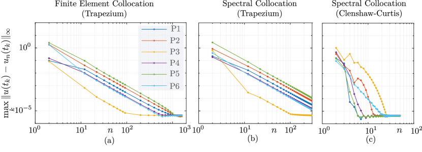
Figure 1: Convergence of (a) the Finite Element Collocation scheme of Section 4.1.1 with Composite Trapezium Quadrature, (b) the Spectral Collocation scheme of Section 4.1.2 with Composite Trapezium Quadrature, and (c) the same Spectral Collocation scheme with Clenshaw–Curtis quadrature, on test problems P1–P6. In (a) and (c) a quadrature scheme that matches the accuracy of the projector has been selected, and gives convergence at the projector’s rate. In (b) the scheme displays $O(n^{-2})$ convergence, even though the projector has a faster convergence rate, because the error is dominated by the $O(n^{-2})$ error of the composite trapezium quadrature.

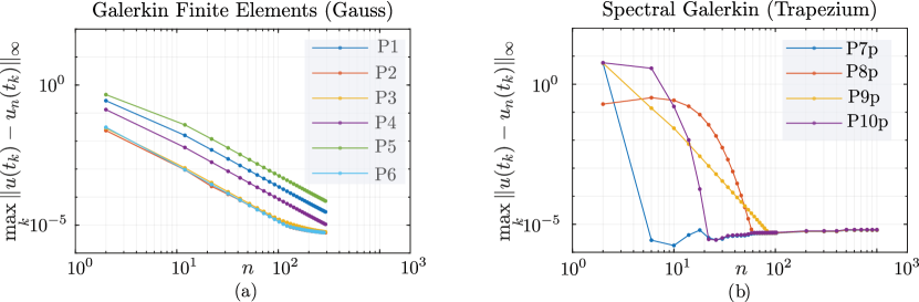
Figure 2: Convergence of (a) the Galerkin Finite Elements scheme of Section 4.2.1 with Gauss quadrature for problems P1–P6 and (b) the Spectral Galerkin scheme of Section 4.2.2 on spatially-periodic problems P7p–P10p.

We tested the schemes described above using neural field equations with a solution in closed form. We use a common firing rate function function $f$ with explicit inverse, and a kernel with product structure:

$$f(u)=\frac{1}{1+e^{-k(u-\theta)}},\qquad f^{-1}(u)=\theta-\frac{1}{k}\log\frac{1-u}{u},\qquad w(x,y)=\exp(-x^{2}+y^{2})\zeta(y).$$

With these choices, $u_{*}(x,t)=f^{-1}(D\exp(-\gamma t-x^{2}))$, for $D\in(0,1)$, solves the neural field problem on $\Omega=[-1,1]$ with external input given by

$$\xi(x,t)=\partial_{t}u_{*}(x,t)+u_{*}(x,t)-\zeta_{0}f(u_{*}(x,t)),\qquad\zeta_{0}= \int_{-1}^{1}\zeta(y)\,dy,$$

and has therefore a closed-form expressions for suitable functions $\zeta(y)$. A similar strategy was chosen for exact solutions to periodic problems. In particular, we kept $f$ as before, and selected kernel and exact solutions as follows:

$$w_{p}(x,y)=\exp(-\cos^{2}x+\cos^{2}y)\zeta_{p}(y),\qquad u_{*p}(x,y)=f^{-1}(D\exp(-\gamma t-\cos^{2}x)),$$

which give an exact solution to the neural field problem on $\Omega=\mathbb{R}/2\pi\mathbb{Z}$ for

$$\xi_{p}(x,t)=\partial_{t}u_{*p}(x,t)+u_{*p}(x,t)-\zeta_{0p}f(u_{*p}(x,t)),\qquad\zeta_{0p}= \int_{-\pi}^{\pi}\zeta_{p}(y)\,dy.$$

By varying functions $\zeta$, $\zeta_{p}$ we obtained 10 test problems: 6 posed on $\Omega=[-1,1]$ and labelled P1–P6, and 4 posed on $\Omega=\mathbb{R}/2\pi\mathbb{Z}$, labelled P7p–P10p. Parameters for the tests are given in Table 1 in Appendix F. For the time discretisation we used an explicit Runge–Kutta (4,5) formula, the Dormand–Prince pair implemented in Matlab’s in-built ode45 routine, with default tolerance parameters. We tested several discrete schemes, by combining Collocation or Galerkin schemes with quadrature rules. Detailed expressions for the discrete schemes, and implementation details are given in Appendix F. Codes are hosted on a public repository, and all numerical experiments in the paper can be modified and run with a single click without a Matlab license, using the following coding capsule [10].

Before presenting the results, we recall that the numerical experiments presented below use numerical schemes that slightly differ from the ones analysed in Section 3 because: (i) a time stepper is employed for the time discretisation and (ii) a quadrature rule is chosen to approximate integrals. The discussions in Sections 3.1 and 5 point to a total error bounded by three contributions $E_{\textrm{timestep}}+E_{\textrm{projection}}+E_{\textrm{quadrature}}$. We do not yet have a convergence result for the Runge–Kutta (4,5) pair implemented in Matlab, and for all the quadrature rules presented below, but the convergence results in Sections 1 and 3 predict convergence rates when the timestepper error is negligible and the quadrature error matches asymptotically the projection error, as we will now discuss.

Finite Element Collocation with Trapezium quadrature. We implemented the method described in Section 4.1.1, with $O(h_{x}^{2})$ convergence, with the composite trapezium quadrature scheme, which preserves this order of accuracy. This scheme is the most prominently used in the mathematical neuroscience literature. Figure 1(a) shows the expected $O(n^{-2})$ convergence of the $C(J,C^{2}([-1,1]))$ error for problems P1–P6. From Fig. 1(a) we observe that the timestepper error dominates when the $C(J,C^{2}([-1,1]))$ error is of the order of $10^{-5}$, and this will be true henceforth for other experiments too. Figure 1(a) indicates that, when $E_{\textrm{timestepper}}$ is dominated by $E_{\textrm{projection}}+E_{\textrm{quadrature}}$ and the latter errors are $O(n^{-2})$, then the total error is an $O(n^{-2})$, as predicted by Corollary 4.2. This is also confirmed by the observation that, when the tolerance of the time stepper is tightened, the plateau in Fig. 1(a) shifts from $10^{-5}$to a lower value (not shown, but verifiable via the code capsule [10]).

Chebyshev Spectral Collocation with Trapezium and Clenshaw–Curtis quadrature. The scheme of Section 4.1.2 has been tested on problems P1-P6. For these examples we expect a faster than quadratic convergence, for sufficiently smooth kernels, provided the chosen quadrature scheme preserves this rate. In passing, we note that the integrands $\zeta$ for P1–P6 are taken from Figure 2 in [49], where the accuracy of Clenshaw–Curtis quadrature is analysed for such functions. We first implemented a discrete scheme with a composite trapezium rule. From Fig. 1(b) it is clear that the $O(n^{-2})$ rate of the quadrature pollutes the overall convergence. We then switched to Clenshaw–Curtis quadrature, which uses Chebyshev points also as quadrature nodes, has excellent convergence properties for this setup [49], and can be implemented with Fast Fourier Transforms (FFTs). Fig. 1(c) shows the superior convergence properties of this scheme, as predicted by Corollary 4.4. At the time of writing we are unaware of research papers where neural fields are simulated using the Chebyshev Spectral Collocation with Clenshaw–Curtis quadrature, which is the most accurate and efficient scheme between the ones presented here for non-periodic domains.

Finite Element Galerkin with Trapezium and Gauss quadrature. We derived from the $O(h_{x}^{2})$-convergent scheme of Section 4.2.1 two discrete schemes, and tested them on P1-P6. In the first one we use composite Trapezium quadrature to approximate the integral operator as well as all inner products, including the ones for the mass matrix $\langle\ell_{i},\ell_{j}\rangle$ which could be computed in closed form. In Section F.3 we explain that the scheme so derived does not require inner product evaluations, and in fact coincides with the discrete Finite-Element Collocation scheme seen in Fig. 1(a). We also derived a second discrete scheme, where the mass matrix is in closed form, (and must be inverted at every function evaluation) and we use Gauss quadrature on reference elements with $2$ nodes. This scheme’s $O(n^{-2})$ convergence rate is seen in Fig. 2(a), even though it is less efficient than the one with Trapezium quadrature which does not require inner products, as explained in Section F.3. The findings in Fig. 2(a) are thus in line with Proposition 4.7.

Spectral Galerkin scheme with Trapezium quadrature. Finally we derived a discrete spectral Galerkin scheme from Section 4.2.2, using trapezium quadrature, which is well suited for periodic integrands [51]. We proceed with a pseudospectral evaluation of the right-hand side, which can be performed with a forward and backward FFT call. The fast convergence of the scheme is reported in Fig. 2(b) for periodic problems P7p–P10p (see discussion in Section 4.2.2 for expected convergence rates). In passing we note that further efficiency savings can be obtained if the neural field has a convolutional structure, as it was shown in [47] for a collocation scheme with pseudoscpetral evaluation of the right-hand side.

7 Conclusions

We have shown that projection methods in use for Fredholm integral equations can be employed successfully in time-dependent neural field equations. As in the stationary theory, convergence properties of the projector determine the convergence rate of the scheme, and guide the choice of quadrature rules in discrete methods.

The theory presented here is applicable to generic domains in $\mathbb{R}^{d}$, and we envisage that further extensions may lead to the adoption of projection schemes on realistic cortices. In particular, it seems straightforward to adapt the methods described here to the case of multiple neuronal populations. This requires the definition of the problem on a different Banach space with respect to the ones adopted here [24], and involves a bounded linear operator $L$ in place of the operator $-\operatorname{Id}_{\mathbb{X}}$ which gives the linear part of Eq. 1. The adaptation seems to require the use of a uniformly continuous semigroup $e^{Lt}$ in place of $e^{-t}$, used in this paper. In addition, with suitable modifications, we envisage that projection methods can be used for neural fields of new generation which have a different nonlocal evolution equation, but have already been simulated with collocation or Galerkin schemes [15, 48].

It may also be possible to extend the projection method characterisation to neural fields with delays for which discrete Galerkin methods exist [44]. When delays are present, the initial Cauchy problem Eq. 11 with $t_{0}=0$, for instance, is replaced by a functional equation in $C([-\tau,0],\mathbb{X})$ [53, 27, 44], with $\tau$ being a maximal delay. A theory that blends projection methods and recent progress on sun-star calculus [30, 31] is unexplored, nontrivial, and relevant for applications.

The adoption of projection methods on large scale problems continues to pose the challenge of evaluating right-hand sides with large and dense matrices. One direction that we are currently investigating is the adoption of multi-resolution bases [18], which lead to fast methods for stationary problems, and can seemingly be ported to neural fields, thereby requiring only $O(n\log n)$ function evaluations. Also, we have not investigated in this paper the stability of timesteppers for neural fields, or a posteriori error bounds, which are important for spatial and temporal adaptation of the schemes. We hope that this article will stimulate the development of such techniques, and the rigorous study of numerical approximations for spatially-extended neuroscience problems.

Appendix A Proof of Lemma 2.1

Proof A.1.

Let $\mathbb{X}=C(\Omega)$. If $u\in C(\Omega)$, then by Section 2 $f(u)\in C(\Omega)$ and $|f(u)|\leq\|f\|_{\infty}$, hence $F\colon\mathbb{X}\to\mathbb{X}$, $F$ is bounded, and Eq. 7 holds. To prove that $F$ is Lipschitz, fix $x\in\Omega$; by Section 2 and the Mean Value Theorem there exists $z(x)\in(u(x),v(x))$ such that

(53) $$|f(u(x))-f(v(x))|\leq|f^{\prime}(z(x))|\;|u(x)-v(x)|\leq\|f^{\prime}\|_{\infty}|u(x)-v(x)|,$$

thus Eq. 9 holds with $\|{\mkern 2.0mu\cdot\mkern 2.0mu}\|=\|{\mkern 2.0mu\cdot\mkern 2.0mu}\|_{\infty}$.

Let us now turn to the case $\mathbb{X}=L^{2}(\Omega)$. To prove that $F$ maps $L^{2}(\Omega)$ to itself see for instance [40, Lemma 3.30]: for any $u\in L^{2}(\Omega)$, we have

$$\|F(u)\|^{2}_{L^{2}(\Omega)}=\int_{\Omega}|f(u(x))|^{2}\,dx\leq|\Omega|\;\|f\|^{2}_{\infty}.$$

thus $F\colon L^{2}(\Omega)\to L^{2}(\Omega)$, and Eq. 7 holds. From Eq. 53 we obtain

$$\|F(u)-F(v)\|^{2}_{L^{2}(\Omega)} =\int_{\Omega}|f(u(x))-f(v(x))|^{2}\,dx$$

$$\leq\|f^{\prime}\|^{2}_{\infty}\int_{\Omega}|u(x)-v(x)|^{2}\,dx$$

$$=\|f^{\prime}\|^{2}_{\infty}\|u-v\|^{2}_{L^{2}(\Omega)}$$

which gives Eq. 9.

Appendix B Proof of Lemma 2.3

Proof B.1.

The operator $W$ is clearly linear. If $\mathbb{X}=C(\Omega)$, then Section 2 implies compactness (hence boundedness) of $W\colon C(\Omega)\to C(\Omega)$ and $\|W\|=\kappa_{w}$ (see [7, Section 2.8.1] and [6, Section 1.2]).

We then turn to the case $\mathbb{X}=L^{2}(\Omega)$. By Section 2 $w\in L^{2}(\Omega\times\Omega)$, hence $W$ is a Hilbert-Schmidt operator, and this implies the compactness of $W$ (see, for instance [6, Section 1.2] or [28, online Chapter 8]). Take $v\in L^{2}(\Omega)$ and set $z=Wv$. Since $w\in L^{2}(\Omega\times\Omega)$, then $w(x,{\mkern 2.0mu\cdot\mkern 2.0mu})\in L^{2}(\Omega)$ for almost all $x\in\Omega$. Thus, $w(x,{\mkern 2.0mu\cdot\mkern 2.0mu})v({\mkern 2.0mu\cdot\mkern 2.0mu})$ is integrable (and $z$ well defined) for almost all $x\in\Omega$. Using standard definitions and the Cauchy-Schwarz inequality we have

$$\|Wu\|^{2}_{L^{2}(\Omega)} =\int_{\Omega}\bigg{|}\int_{\Omega}w(x,y)u(y)\,dy\bigg{|}^{2}\,dx$$

$$=\int_{\Omega}\langle w(x,{\mkern 2.0mu\cdot\mkern 2.0mu}),u\rangle^{2}_{L^{2}(\Omega)}\,dx$$

$$\leq\int_{\Omega}\|w(x,{\mkern 2.0mu\cdot\mkern 2.0mu})\|^{2}_{L^{2}(\Omega)}\|u\|^{2}_{L^{2}(\Omega)}\,dx$$

$$=\|u\|^{2}_{L^{2}(\Omega)}\int_{\Omega}\int_{\Omega}|w(x,y)|^{2}\,dy\,dx=\|w\|^{2}_{L^{2}(\Omega\times\Omega)}\|u\|^{2}_{L^{2}(\Omega)},$$

which gives $\kappa_{w}$ when $\mathbb{X}=L^{2}(\Omega)$.

Appendix C Proof of Lemma 2.5

Proof C.1.

Fix $b>0$, and consider a sequence $\{(t_{n},u_{n})\}_{n\in\mathbb{N}}\in Q_{b}$ such that $(t_{n},u_{n})\to(t,u)$ as $n\to\infty$. We prove the continuity of $N$ by showing $N(t_{n},u_{n})\to N(t,u)$ as $n\to\infty$ in $\mathbb{X}$, that is, for any $\varepsilon>0$, there exists an integer $m$ such that

$$\|N(t_{n},u_{n})-N(t,u)\|\leq\varepsilon\quad\text{for all $n\geq m$.}$$

Fix $\varepsilon>0$. The convergence of $(t_{n},u_{n})$ to $(t,u)$, the Lipschitz continuity (and hence continuity) of $F$ (see Lemma 2.1), and Section 2 imply the existence of integers $m_{1}$, $m_{2}$, $m_{3}$ such that

$$\|u_{n}-u\|\leq\varepsilon/3, n\geq m_{1}$$ for all ,

$$\|F(u_{n})-F(u)\|\leq\varepsilon/(3\kappa_{w}), n\geq m_{2}$$ for all ,

$$\|\xi(t_{n})-\xi(t)\|\leq\varepsilon/3, n\geq m_{3}$$ for all ,

respectively, hence for all $n\geq m=\max(m_{1},m_{2},m_{3})$.

$$\|N(t_{n},u_{n})-N(t,u)\|\leq\|u_{n}-u\|+\kappa_{w}\|F(u_{n})-F(u)\|+\|\xi(t_{n})-\xi(t)\|\leq\varepsilon$$

We now proceed to check the Lipschitz continuity of $N$. Using the Lipschitz continuity of $F$ (see Lemma 2.1) we obtain for any $(t,u),(t,v)\in Q_{b}$

$$\|N(t,u)-N(t,v)\|\leq\|u-v\|+\|W\|\|F(u)-F(v)\|\leq(1+\kappa_{w}\|f^{\prime}\|_{\infty})\|u-v\|$$

therefore $N$ is Lipschitz continuous in the second argument, uniformly with respect to the first, because its Lipschitz constant is independent of $t$.

Appendix D Proof of Theorem 3.1

Proof D.1.

The proof follows closely the steps in Lemmas 2.5 and 2.7. Let

$$Q_{b}=\{(t,u)\in\mathbb{R}\times\mathbb{X}_{n}\colon|t-t_{0}|\leq T,\quad\|u-u_{0}\|\leq b\}.$$

The boundedness of $P_{n}$ implies that $P_{n}N\colon Q_{b}\to\mathbb{X}_{n}$ is continuous, and Lipschitz continuous in its second argument, uniformly with respect to the first. Applying Theorem 5.2.4 in [7] we obtain the existence and uniqueness of a solution $u_{n}\in C^{1}(J,\mathbb{X}_{n})$ to Eq. 14 with initial condition $u_{n}(t_{0})=P_{n}u_{0}\in\mathbb{X}_{n}$.

Appendix E Proof of Lemma 3.7

Proof E.1.

From the evolution equation Eq. 14 and Lemma 2.1 we obtain

$$\|u^{\prime}_{n}(t)\|\leq\|u_{n}(t)\|+\kappa_{\Omega}\|P_{n}W\|\|f\|_{\infty}+\|P_{n}\xi(t)\|,$$

and Eq. 23 follows from $u_{n},P_{n}\xi\in C(J,\mathbb{X})$. The hypotheses on $W$ and $F$ guarantee that the operator $K\colon\mathbb{X}\to\mathbb{X}$, $u\mapsto WF(u)$ is Fréchet differentiable with derivative

$$K^{\prime}(u)\colon\mathbb{X}\to\mathbb{X},\qquad v\mapsto\int_{\Omega}W({\mkern 2.0mu\cdot\mkern 2.0mu},y)f^{\prime}(u(y))v(y)\,dy.$$

We obtain

$$u^{\prime\prime}_{n}(t)=-u^{\prime}_{n}(t)+P_{n}K^{\prime}(u_{n}(t))u^{\prime}_{n}(t)+P_{n}\xi^{\prime}(t),$$

hence

$$\|u^{\prime\prime}_{n}(t)\|\leq L_{n}\|u^{\prime}_{n}(t)\|+\|P_{n}\xi^{\prime}(t)\|$$

and Eq. 24 holds because $u^{\prime}_{n},P_{n}\xi^{\prime}\in C(J,\mathbb{X})$. The bound Eq. 24 implies $u_{n}\in C^{2}(J,\mathbb{X})$.

The existence of $\kappa_{1},\kappa_{2}$ in Eq. 25 follows directly if $P_{n}v\to v$ for all $v\in\mathbb{X}$. Under this hypothesis: (i) by Theorem 3.3 $u_{n}\to u$ in ${C(J,\mathbb{X})}$, hence the sequence with elements $\|u_{n}\|_{C(J,\mathbb{X})}$ is bounded; (ii) the same arguments used in the proof of Theorem 3.3, in the discussion leading to Eq. 20, give $\|W-P_{n}W\|\to 0$, hence the sequences $\{\gamma_{n}\}$ and $\{L_{n}\}$ are bounded; (iii) $\xi\in C(J,\mathbb{X})$ implies the uniform convergence of $\{P_{n}\xi\}$ to $\xi$, hence the sequence with elements $\|P_{n}\xi\|_{C(J,\mathbb{X})}$ is bounded; (iv) a similar argument on $\xi^{\prime}\in C(J,\mathbb{X})$ implies that the sequence with elements $\|P_{n}\xi\|_{C(J,\mathbb{X})}$ is bounded.

Appendix F Implementation of discrete schemes

Table 1: Parameters for test neural field problems with exact solutions.

Problem	$D$	$\gamma$	$k$	$\theta$	$\zeta(y)$ or $\zeta_{p}(y)$
P1	0.8	0.5	5	0.3	$\exp{y}\cos y$
P2	-	-	-	-	$y^{20}$
P3	-	-	-	-	$(1+16y^{2})^{-1}$
P4	-	-	-	-	$\exp(-y^{2})$
P5	-	-	-	-	$\exp(-y)$
P6	-	-	-	-	$|y|^{3}$
P7p	-	-	-	-	$\cos^{2}y$
P8p	-	-	-	-	$(1+16\cos^{2}y)^{-1}$
P9p	-	-	-	-	$|\cos^{3}y|$
P10p	-	-	-	-	$\cos^{20}y$

F.1 Finite Element Collocation with Trapezium quadrature

In a first numerical test we implemented the method described in Section 4.1.1. Since the scheme converges as $O(h_{x}^{2})$, we selected the composite trapezium quadrature scheme, which preserves this order of accuracy. This leads to the set of ODEs

(54) $$a^{\prime}_{i}(t)=-a_{i}(t)+\sum_{j=0}^{n}W_{ij}f(a_{j}(t))+\xi(x_{i},t),\qquad a_{i}(0)=u_{0}(x_{i},0),\qquad i\in\mathbb{Z}_{n+1}$$

where

$$W_{ij}=w(x_{i},x_{j})\rho_{j},\qquad\rho_{j}=\begin{cases}h_{x}&\text{for $j\in\mathbb{N}_{n-1}$,}\\ h_{x}/2&\text{for $j\in\{0,n\}$.}\end{cases}$$

F.2 Chebyshev Spectral Collocation with Trapezium and Clenshaw–Curtis quadrature

We have used Trapezium and Clenshaw–Curtis quadrature for the spectral collocation scheme of Section 4.1.2. In the former, we discretised the integrals in Eq. 36 using the composite trapezium rule, and arriving at a discrete system analogous to Eq. 54, but where $\{x_{i}\}$ indicate the $n+1$ Chebyshev nodes Eq. 34, and where a set of different $n+1$ quadrature nodes $\{z_{i}\}$ are taken to be evenly spaced by $h_{x}$, giving

$$W_{ij}=w(x_{i},z_{j})\rho_{j},\qquad\rho_{j}=\begin{cases}h_{x}&\text{for $j\in\mathbb{N}_{n-1}$,}\\ h_{x}/2&\text{for $j\in\{0,n\}$.}\end{cases}$$

Secondly, we implemented a scheme with Clenshaw–Curtis quadrature. In this case, we form the matrix with elements $W(x_{i},x_{j})\rho_{j}$, where $\{x_{i}\}$ are the Chebyshev nodes and $\rho_{j}$ the Clenshaw–Curtis weights. The scheme is written as

(55) $$\bm{a}^{\prime}(t)=-\bm{a}(t)+\bm{W}\bm{f}(\bm{a}(t))+\bm{\xi}(t),\qquad\bm{a}(0)=\bm{u_{0}}(0).$$

The matrix-vector product on the right-hand side, however, is evaluated calling $n+1$ times the FFT of an $(n+1)$-vector (see the accompanying codes [10] where we have adapted for integrals the scripts in [49]).

F.3 Finite Element Galerkin scheme with Gauss quadrature

. We used P1-P6 to test the Finite Element Galerkin scheme with piecewise-linear hat functions, discussed in Section 4.2.1. The spatially-continuous scheme contains a sparse mass matrix with entries $M_{ij}=\langle\ell_{i},\ell_{j}\rangle_{L^{2}(-1,1)}$, computable in closed form [6, Section 3.3.1]. The scheme is

$$\sum_{j=0}^{n}M_{ij}a^{\prime}_{j}(t)=-\sum_{j=0}^{n}M_{ij}a_{j}(t) +\int_{-1}^{1}\ell_{i}(x)\int_{-1}^{1} w(x,y)f\Big{(}\sum_{k=0}^{n}a_{k}(t)\ell_{k}(y)\Big{)}\,dy\,dx$$

$$+\int_{-1}^{1}\ell_{i}(x)\xi(x,t)\,dx$$

Since, by the projector error, this scheme converges to $O(h_{x}^{2})$, one possibility to obtain a matching discrete method is to use the composite Trapezium rule. In this case, it is advantageous to pair it to a so-called mass-lumping procedure [46, Section 13.3, page 595], which uses the Trapezium rule also to evaluate the components of $M_{ij}$. Since by the Trapezium rule $M_{ij}=\rho_{i}\delta_{ij}+O(h_{x}^{2})$, this allows us to pass from a sparse mass matrix, which must be inverted to evaluate the right-hand side, to a new problem with an approximate, but diagonal mass matrix,

$$\rho_{i}a^{\prime}_{i}(t)=-\rho_{i}a_{i}(t)+\rho_{i}\sum_{j=0}^{n}W_{ij}f(a_{j}(t))+\rho_{i}\xi(x_{i},t),\qquad a_{i}(0)=u_{0}(x_{i},0),\qquad i\in\mathbb{Z}_{n+1}$$

where $\rho_{i}$ are the composite Trapezium weights. This discrete scheme uses the fact that the inner products and integral operator on the right-hand side are approximated at $O(h_{x}^{2})$, that the projection scheme (before discretisation) converges to $O(h_{x}^{2})$, and hence one can tolerate the same error on $M_{ij}$. The main advantage is that, once each equation is divided by the nonzero weights $\rho_{i}$, this scheme is identical to the discrete Finite Element collocation scheme Eq. 54, therefore it does not require, in practice, any inner product integration. Numerical convergence results for this scheme are therefore given in Fig. 1(a).

An alternative is to proceed as in classical Finite Element methods, and pair the hat functions $\{\ell_{i}\}$ with a Gaussian quadrature rule

$$\int_{-1}^{1}\psi(x)\,dx\approx\sum_{q=1}^{n_{q}}\psi(z_{q})\nu_{q}.$$

For this scheme one introduces reference hat functions and coordinate mappings

$$\varphi_{\pm}(z)=\frac{1\pm z}{2},\qquad g_{i}:[-1,1]\to\Omega_{i},\quad g_{i}(z)=x_{i}+\frac{(1+z)(x_{i+1}-x_{i})}{2},i\in\mathbb{N}_{n}$$

and derive the following discrete scheme

$$\sum_{j=0}^{n}M_{ij}a^{\prime}_{j}(t)=-\sum_{j=0}^{n}M_{ij}a_{j}(t)+\frac{h}{2}\sum_{q=1}^{n_{q}}\bigg{[}\varphi_{-}(z_{q})v(g_{i}(z_{q}),t)\nu_{q}+\varphi_{+}(z_{q})v(g_{i+1}(z_{q}),t)\nu_{q}\bigg{]}$$

where

$$v(x,t)=\xi(x,t)+\frac{h}{2}\sum_{j=1}^{n}\sum_{q=1}^{n_{q}}w(x,g_{j}(z_{q}))f(a_{j}\varphi^{-}(z_{q})+a_{j+1}\varphi^{+}(z_{q}))\nu_{q}.$$

This scheme has been implemented for a Gaussian quadrature scheme with $n_{q}=2$, and its convergence properties are seen in Fig. 2(a).

F.4 Spectral Galerkin Scheme with Trapezium Quadrature

As a final test, we implemented the spectral Galerkin scheme of Section 4.2.2. We rewrite the scheme as

(56) $$a^{\prime}_{i}(t)= -a_{i}(t)+\int_{\Omega}\varphi_{i}(x)v^{*}(x,t)\,dx$$

$$a_{i}(t_{0})= \int_{\Omega}\varphi_{i}(x)u^{*}_{0}(x)\,dx$$

where

$$v(x,t)=\xi(x,t)+\int_{\Omega}w(x,y)f\bigg{(}\sum_{j\in\mathbb{Z}_{n+1}}a_{j}(t)\varphi_{j}(y)\bigg{)}\,dy\,dx$$

Since the integrand in the expression for $v$ is periodic, we selected for this scheme a composite trapezium rule, which is well suited for periodic integrands [51]. In addition, the integrals in Eq. 56 cam be evaluated using the FFT. We have implemented this scheme combining Fast Fourier Transform with a pesudospectral evaluation of the integrands in $v$. More specifically, the scheme can be expressed compactly in vector notation, using forward and backward Discrete Fourier Transforms operators for vectors, as follows

$$\bm{a}^{\prime}(t) =-\bm{a}(t)+\mathcal{F}\Big{[}\bm{\xi}(t)+h_{x}\bm{W}\bm{f}\big{(}\mathcal{F}^{-1}[\bm{a}(t)]\big{)}\Big{]},$$

$$\bm{a}(0) =\mathcal{F}[\bm{u}_{0}].$$

References

- [1] H. Amann, Ordinary differential equations: an introduction to nonlinear analysis, vol. 13, Walter de gruyter, 2011.
- [2] S.-i. Amari, Dynamics of pattern formation in lateral-inhibition type neural fields, Biological Cybernetics, 27 (1977), pp. 77–87.
- [3] P. M. Anselone, Collectively compact operator approximation theory and applications to integral equations, Prentice hall, Prentice Hall, Dec. 1971. tex.rating: 0.
- [4] K. E. Atkinson, The Numerical Evaluation of Fixed Points for Completely Continuous Operators, SIAM Journal on Numerical Analysis, 10 (1973), pp. 799–807.
- [5] K. E. Atkinson, A Survey of Numerical Methods for Solving Nonlinear Integral Equations, Journal of Integral Equations and Applications, 4 (1992), pp. 15–46.
- [6] K. E. Atkinson, The Numerical Solution of Integral Equations of the Second Kind, Cambridge Monographs on Applied and Computational Mathematics, Cambridge University Press, 1997, https://doi.org/10.1017/CBO9780511626340.
- [7] K. E. Atkinson and W. Han, Theoretical numerical analysis, vol. 39, Springer, 2005.
- [8] K. E. Atkinson and F. A. Potra, Projection and Iterated Projection Methods for Nonlinear Integral equations, SIAM Journal on Numerical Analysis, 24 (1987), pp. 1352 – 1373, https://doi.org/10.1137/0724087.
- [9] D. Avitabile, Numerical Computation of Coherent Structures in Spatially- Extended Systems, May 2020, https://doi.org/10.5281/zenodo.3821169, https://doi.org/10.5281/zenodo.3821169.
- [10] D. Avitabile, Projection methods for neural field equations. https://www.codeocean.com/, 11 2021, https://doi.org/10.24433/CO.3131389.v1.
- [11] D. Avitabile, S. Coombes, and P. M. Lima, Numerical investigation of a neural field model including dendritic processing, Journal of Computational Dynamics, 7 (2020), pp. 271–290, https://doi.org/10.3934/jcd.2020011.
- [12] Z. Battles and L. N. Trefethen, An Extension of MATLAB to Continuous Functions and Operators, SIAM Journal on Scientific Computing, 25 (2004), pp. 1743–1770, https://doi.org/10.1137/s1064827503430126.
- [13] J.-P. Berrut and L. N. Trefethen, Barycentric Lagrange Interpolation, SIAM Review, 46 (2004), pp. 501–517, https://doi.org/10.1137/s0036144502417715.
- [14] P. C. Bressloff, Waves in Neural Media, Springer New York, Springer New York, 2014, https://doi.org/10.1007/978-1-4614-8866-8.
- [15] Á. Byrne, D. Avitabile, and S. Coombes, Next-generation neural field model: The evolution of synchrony within patterns and waves, Physical Review E, 99 (2019), p. 012313.
- [16] P. C., Bressloff, Spatiotemporal dynamics of continuum neural fields, Journal of Physics A: Mathematical and Theoretical, 45 (2012), p. 033001, https://doi.org/10.1088/1751-8113/45/3/033001.
- [17] C. Canuto, M. Y. Hussaini, A. Quarteroni, and T. A. Zang, Spectral Methods, Fundamentals in Single Domains, Scientific Computation, Springer-Verlag, Berlin, 2006, https://doi.org/10.1007/978-3-540-30726-6.
- [18] Z. Chen, C. A. Micchelli, and Y. Xu, Multiscale Methods for Fredholm Integral Equations, Cambridge University Press, July 2015.
- [19] S. Coombes, P. beim Graben, R. Potthast, and J. Wright, Neural fields: theory and applications, Springer, 2014.
- [20] B. Ermentrout, Neural networks as spatio-temporal pattern-forming systems, Reports on Progress in Physics, 61 (1998), pp. 353 – 430, https://doi.org/10.1088/0034-4885/61/4/002.
- [21] G. B. Ermentrout and D. H. Terman, Mathematical Foundations of Neuroscience, vol. 35 of Interdisciplinary Applied Mathematics, Springer New York, 2010, https://doi.org/10.1007/978-0-387-87708-2.
- [22] O. Faugeras, F. Grimbert, and J.-J. Slotine, Absolute stability and complete synchronization in a class of neural fields models, SIAM Journal on applied mathematics, 69 (2008), pp. 205–250.
- [23] O. Faugeras and J. Inglis, Stochastic neural field equations: a rigorous footing, Journal of Mathematical Biology, 71 (2015), pp. 259–300, https://doi.org/10.1007/s00285-014-0807-6.
- [24] O. Faugeras, R. Veltz, and F. Grimbert, Persistent Neural States: Stationary Localized Activity Patterns in Nonlinear Continuous n-Population, q-Dimensional Neural Networks, Neural Computation, 21 (2009), pp. 147–187.
- [25] G. Faye and O. Faugeras, Some theoretical and numerical results for delayed neural field equations, Physica D, 239 (2010), pp. 561 – 578, https://doi.org/10.1016/j.physd.2010.01.010.
- [26] S. E. Folias and P. C., Bressloff, Breathers in Two-Dimensional Neural Media, Physical Review Letters, 95 (2005), p. 208107.
- [27] S. A. v. Gils, S. G. Janssens, Y. A. Kuznetsov, and S. Visser, On local bifurcations in neural field models with transmission delays, Journal of Mathematical Biology, 66 (2013), pp. 837 – 887, https://doi.org/10.1007/s00285-012-0598-6.
- [28] C. Heil, Metrics, Norms, Inner Products, and Operator Theory, Springer, 2018.
- [29] A. Hutt, Local excitation-lateral inhibition interaction yields oscillatory instabilities in nonlocally interacting systems involving finite propagation delay, Physics Letters A, 372 (2008), pp. 541–546, https://doi.org/10.1016/j.physleta.2007.08.018.
- [30] S. G. Janssens, A class of abstract delay differential equations in the light of suns and stars, Tech. Report arXiv:1901.11526, arXiv, Jan. 2019, https://doi.org/10.48550/arXiv.1901.11526, http://arxiv.org/abs/1901.11526 (accessed 2022-10-03). arXiv:1901.11526 [math] type: article.
- [31] S. G. Janssens, A class of abstract delay differential equations in the light of suns and stars. II, Tech. Report arXiv:2003.13341, arXiv, Mar. 2020, https://doi.org/10.48550/arXiv.2003.13341, http://arxiv.org/abs/2003.13341 (accessed 2022-10-03). arXiv:2003.13341 [math] type: article.
- [32] Z. P. Kilpatrick and B. Ermentrout, Wandering bumps in stochastic neural fields, SIAM Journal on Applied Dynamical Systems, 12 (2013), pp. 61–94.
- [33] C. Kuehn and M. G. Riedler, Large Deviations for Nonlocal Stochastic Neural Fields, The Journal of Mathematical Neuroscience, 4 (2014), p. 1, https://doi.org/10.1186/2190-8567-4-1, http://mathematical-neuroscience.springeropen.com/articles/10.1186/2190-8567-4-1 (accessed 2022-03-21).
- [34] S. Kumar, A discrete collocation-type method for hammerstein equations, SIAM journal on numerical analysis, 25 (1988), pp. 328–341.
- [35] S. Kumar and I. H. Sloan, A new collocation-type method for hammerstein integral equations, Mathematics of computation, (1987), pp. 585–593.
- [36] C. R. Laing, Numerical bifurcation theory for high-dimensional neural models, The Journal of Mathematical Neuroscience, 4 (2014), pp. 1–27.
- [37] P. S. Leon, S. A. Knock, M. M. Woodman, L. Domide, J. Mersmann, A. R. McIntosh, and V. Jirsa, The Virtual Brain: a simulator of primate brain network dynamics, Frontiers in Neuroinformatics, 7 (2013), p. 10, https://doi.org/10.3389/fninf.2013.00010.
- [38] P. M. Lima, Numerical investigation of stochastic neural field equations, in Advances in Mathematical Methods and High Performance Computing, Springer, 2019, pp. 51–67.
- [39] P. M. Lima and E. Buckwar, Numerical Solution of the Neural Field Equation in the Two-Dimensional Case, SIAM Journal on Scientific Computing, 37 (2015), pp. B962–B979, https://doi.org/10.1137/15m1022562.
- [40] G. J. Lord, C. E. Powell, and T. Shardlow, An introduction to computational stochastic PDEs, Cambridge University Press, Cambridge, Jan. 2014.
- [41] J. N. MacLaurin and P. C. Bressloff, Wandering bumps in a stochastic neural field: A variational approach, Physica D: Nonlinear Phenomena, 406 (2020), p. 132403.
- [42] R. Martin, D. J. Chappell, N. Chuzhanova, and J. J. Crofts, A numerical simulation of neural fields on curved geometries, Journal of Computational Neuroscience, 45 (2018), pp. 133–145, https://doi.org/10.1007/s10827-018-0697-5, https://doi.org/10.1007/s10827-018-0697-5 (accessed 2022-10-03).
- [43] E. J. Nichols and A. Hutt, Neural field simulator: two-dimensional spatio-temporal dynamics involving finite transmission speed., Frontiers in neuroinformatics, 9 (2015), p. 25, https://doi.org/10.3389/fninf.2015.00025.
- [44] M. Polner, J. J. W. v. d. Vegt, and S. A. v. Gils, A Space-Time Finite Element Method for Neural Field Equations with Transmission Delays, SIAM Journal on Scientific Computing, 39 (2017), pp. B797–B818, https://doi.org/10.1137/16m1085024, https://epubs.siam.org/doi/abs/10.1137/16M1085024?journalCode=sjoce3, https://arxiv.org/abs/1702.07585.
- [45] R. Potthast and P. beim Graben, Existence and properties of solutions for neural field equations, Mathematical Methods in the Applied Sciences, 33 (2010), pp. 935–949.
- [46] A. Quarteroni, R. Sacco, and F. Saleri, Numerical mathematics, vol. 37, Springer Science & Business Media, 2010.
- [47] J. Rankin, D. Avitabile, J. Baladron, G. Faye, and D. J. B. Lloyd, Continuation of localised coherent structures in nonlocal neural field equations, SIAM Journal on Scientific Computing, (2013), SIAMJournalonScientificComputing. 21 pages, 13 figures, submitted for peer review.
- [48] H. Schmidt and D. Avitabile, Bumps and oscillons in networks of spiking neurons, Chaos: An Interdisciplinary Journal of Nonlinear Science, 30 (2020), p. 033133.
- [49] L. N. Trefethen, Is Gauss Quadrature Better than Clenshaw–Curtis?, SIAM Review, 1 (2008), pp. 67–87, https://epubs.siam.org/doi/10.1137/060659831.
- [50] L. N. Trefethen, Approximation Theory and Approximation Practice, Extended Edition, SIAM, 2019.
- [51] L. N. Trefethen and J. Weideman, The exponentially convergent trapezoidal rule, siam REVIEW, 56 (2014), pp. 385–458.
- [52] R. Veltz and O. Faugeras, Local/Global Analysis of the Stationary Solutions of Some Neural Field Equations, SIAM Journal on Applied Dynamical Systems, 9 (2010), pp. 954 – 998, https://doi.org/10.1137/090773611.
- [53] S. Visser, From spiking neurons to brain waves, PhD Thesis, University of Twente, (2013), https://doi.org/10.3990/1.9789036535083, https://research.utwente.nl/en/publications/from-spiking-neurons-to-brain-waves (accessed 2022-10-03).
- [54] S. Visser, R. Nicks, O. Faugeras, and S. Coombes, Standing and travelling waves in a spherical brain model: The Nunez model revisited., Physica D, 349 (2017), pp. 27 – 45, https://doi.org/10.1016/j.physd.2017.02.017.
- [55] H. R. Wilson and J. D. Cowan, A mathematical theory of the functional dynamics of cortical and thalamic nervous tissue, Kybernetik, 13 (1973), pp. 55–80.