Effect of Emitters on Quantum State Transfer in Coupled Cavity Arrays

Abstract

Over the last decade, conditions for perfect state transfer in quantum spin chains have been discovered, and their experimental realizations addressed. In this paper, we consider an extension of such studies to quantum state transfer in a coupled cavity array including the effects of atoms in the cavities which can absorb and emit photons as they propagate down the array. Our model is equivalent to previously examined spin chains in the one-excitation sector and in the absence of emitters. We introduce a Monte Carlo approach to the inverse eigenvalue problem which allows the determination of the inter-cavity and cavity-emitter couplings resulting in near-perfect quantum state transfer fidelity, and examine the time dependent polariton wave function through exact diagonalization of the resulting Tavis-Cummings-Hubbard Hamiltonian. The effect of inhomogeneous emitter locations is also evaluated.

I Introduction

One of the most important questions in quantum information theory is the faithful and rapid, transmission of a quantum state from one location to another. Quantum spin chains have proven to be a very useful and powerful context in which to explore fundamental issues, including the possibility of perfect transfer, the effect of disorder, and the interplay between high fidelity and speed of propagation [1, 2, 3, 4, 5, 6, 7]. In the case where a single excitation is present (one up spin in a background of down spins) the resulting Hamiltonian is represented by a tridiagonal (‘Jacobi’) matrix. A general classification of the eigenspectra of such matrices which result in perfect Quantum State Transfer (QST) has emerged, as has the determination of the requisite ‘fully engineered’ intersite exchange constants $J_{i}$ [2, 3]. Interestingly, it was also found that nearly perfect QST could be achieved with more limited and feasible ‘boundary’ engineering in which the $J_{i}$ are uniform in the interior, and take special values only at the beginning and end of the chain [8]. Although boundary engineering has the advantage of requiring less precise, and therefore less experimentally challenging, tuning, good QST is achieved only in the limit of weak coupling at the ends, and hence is compromised by long transfer times.

A subsequent focus was on the effect of disorder on QST, since in any physical realization a certain degree of randomness is inevitable. There are many eigenvalue distributions which give rise to perfect QST in the ideal limit, and therefore one line of investigation concerned the types of such engineered spectra which are most robust to disorder [9]. A key observation was that once randomness is present, the resulting degradations of state transfer of fully and boundary engineered chains are roughly similar, so that there is limited incentive to attempt full engineering as far as fidelity itself is concerned [10]. (The problem of longer transfer times in boundary engineered chains, however, remains.)

In this paper, we consider QST within a different physical and geometric context, namely when the ‘backbone’ chain also possesses branches to localized qubits, forming a ‘comb-like’ geometry as illustrated in Fig. 1. We are motivated by the study of the nature and propagation of excitations in a coupled cavity array (CCA) [11, 12, 13]. A CCA consists of a chain of optical cavities, which might be empty or may contain one or more atom-like emitters coupled to the cavity’s electromagnetic field. Photons hop between adjacent cavities in the CCA due to the overlap of neighboring resonance modes, and strong interactions between light and matter can be induced. These emitters form the ‘rungs’ which dress our one-dimensional chain of cavities.

CCAs have become increasingly experimentally viable in recent years [14, 15], and have been especially intriguing as possible venues for exploring superfluid to insulator transitions and other many-body phenomena. However, in order to observe such effects, the CCA must exist in the strong coupling regime of cavity quantum electrodynamics, where light-matter interactions are stronger than losses to the environment. Modern integrated optical cavities achieve this by localizing light on the (sub)wavelength scale. One of the commonly used optical resonators for these studies is the photonic crystal cavity, formed by periodic refractive index alteration at the nanoscale.

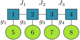
Figure 1: Geometry of the one dimensional Jaynes-Cummings-Hubbard Hamiltonian with $N=4$ cavities each containing $M_{i}=1$ emitter. Photons can ‘hop’ between a set of cavities $i$ and $i+1$ (squares) via the inter-cavity coupling rates $J_{i}$. Within each cavity $i$ a photon can be absorbed and excite the emitter (circles) via $g_{i}$. The same process can be reversed, traveling from emitter to cavity also via $g_{i}$. The numbers indicate our (arbitrary) convention for labeling the states in the Hilbert space, i.e. the rows of our matrix in the single excitation sector.

One of the attractive choices for quasi-atoms which might interact with such solid-state CCAs are color centers formed as lattice defects in semiconductors [16]. The defect causes electron wavefunctions to localize at that point, effectively creating an isolated two-level system within a solid-state material. The most common material substrates for this purpose are silicon carbide [17, 18, 19, 20, 21, 22] and diamond [23, 24, 25, 26].

An immediate question is whether perfect QST is still possible in these more complex ‘two component’ systems, and, if so, what are the associated cavity-cavity and cavity-emitter couplings. A second question pertains to the effect of a fundamentally different type of ‘geometric’ disorder which arises from inhomogeneity in the emitter numbers and locations, rather than the previously explored situations where randomness is introduced via bond-dependent couplings in a fixed and regular geometry. A cavity which is absent an emitter corresponds, for example, to a missing ‘tooth’ at that location of the comb. We will describe the consequences of such disorder on QST.

One interesting aspect of such cavity-emitter arrays is as a novel realization of ‘boundary engineering’. If atoms are placed only in the initial and final positions of $N-2$ cavities, the geometry is identical as that of an $N$ cavity chain. The emitter-cavity couplings then play the role of the bond strengths $J_{1}$ and $J_{N-1}$ of a spin chain.

A final avenue of investigation described here concerns the case of multiple excitations in cavity-emitter systems. In the absence of emitters, the Hamiltonian is quadratic and describes a set of independent bosonic particles (photons). As a consequence, perfect QST in the single excitation sector guarantees the same occurs for multiple excitations. When emitters are present, the Hamiltonian remains quadratic in the photon and emitter operators. However the mixed nature of the commutation relations/allowed ‘occupations’ makes the multi-excitation sector fundamentally different from single excitations. We will describe the prospects for achieving high fidelities in this situation.

Our paper is organized as follows. In Section II we review the Jaynes-Cummings-Hubbard Hamiltonian (JCHH) and its matrix representation in the single excitation sector. We also briefly describe the exact diagonalization method used in the time evolution of states and the Monte Carlo approach used to solve the inverse eigenvalue problem. Section III presents evidence for the possibility of perfect QST in cavity-emitter systems. These results provide ‘full engineering’ solutions to perfect QST in the JCHH, generalizing known spin chain results. Having established perfect QST in this more complex setting, we next consider, in Sec. IV, the effects of disorder. Section V and Sec. VI discuss how cavity emitter systems can provide a novel realization of boundary engineering, and the nature of QST when multiple excitations are present, respectively. A brief overview of experimental parameters in CCA in silicon carbide with color centers serving as emitters is contained in Sec. VII. Finally our results are summarized in Sec. VIII. Several details are discussed in the Appendix.

II Model and Methodology

The cavity-emitter arrays we will study are described by the Jaynes-Cummings-Hubbard Hamiltonian,

$${\cal H} =\sum\limits_{i=1}^{N}\Omega_{i}^{\phantom{\dagger}}a_{i}^{\dagger}a_{i}^{\phantom{\dagger}}+\sum\limits_{i=1}^{N-1}J_{i}^{\phantom{\dagger}}\big{(}\,a_{i+1}^{\dagger}a_{i}^{\phantom{\dagger}}+a_{i}^{\dagger}a_{i+1}^{\phantom{\dagger}}\,\big{)}$$ (1)

$$+\sum\limits_{i=1}^{N}\,\sum\limits_{j=1}^{M_{i}}\omega_{ij}^{\phantom{\dagger}}\sigma_{ij}^{+}\sigma_{ij}^{-}+g_{ij}\big{(}\,a_{i}^{\dagger}\sigma_{ij}^{-}+\sigma_{ij}^{+}a_{i}^{\phantom{\dagger}}\,\big{)}$$

Here $N$ is the number of cavities and $\{M_{i}\}$ are the numbers of emitters in cavity $i$. $a_{i}^{\dagger}\big{(}a_{i}^{\phantom{\dagger}}\big{)}$ are photon creation (annihilation) operators in cavity $i$, and $\sigma_{ij}^{+}\big{(}\sigma_{ij}^{-}\big{)}$ are excitation (de-excitation) operators for emitter $j$ in cavity $i$. The model is parameterized by cavity energies $\Omega_{i}$, photon hopping rates $J_{i}$, emitter energy levels $\omega_{ij}$ and photon-emitter coupling rates $g_{ij}$. We focus on the case when there is at most one emitter per cavity, $M_{i}=0,1$, and hence will simplify the notation to $g_{i}$ and $\omega_{i}$, dropping the $j$ subscript which distinguishes different emitters in the same cavity. In cases when the number of emitters varies, we will refer to the sparse JCHH.

Real cavities and emitters have finite linewidth, representing the possibility of loss. High quality (small linewidth) cavities and emitters are increasingly available [16]. Hence these effects are ignored in the present work.

A basis for the Hilbert space in the single excitation sector and in the absence of emitters is the collection of states $|\,0\,0\,0\,\cdots 0\,1_{i}\,0\cdots 0\,\rangle$ with a single phonon in cavity $i$. The Hamiltonian is represented by the tridiagonal (‘Jacobi’) matrix,

$${{\cal H}=\begin{pmatrix}\Omega_{1}&-J_{1}&0&\ldots&0\\ -J_{1}&\Omega_{2}&-J_{2}&\ldots&0\\ 0&-J_{2}&\Omega_{3}&\ldots&0\\ \vdots&\vdots&\vdots&\ddots&-J_{N-1}\\ 0&0&0&-J_{N-1}&\Omega_{N}\,\,.\end{pmatrix}}$$ (2)

We compute the time evolution from an initial state $|\,\Psi(t=0)\,\rangle$ by diagonalizing ${\cal H}=S\,DS^{\dagger}$, exponentiating ${\cal H}$ to obtain $U=e^{-i{\cal H}t}=S\,e^{-iDt}S^{\dagger}$, thereby finding

$$\ket{\psi(t)}=e^{-i{\cal H}t}\ket{\psi(0)}$$ (3)

where we take $\hbar=1$. We begin our system with $\ket{\psi(0)}=\ket{1,0,0,\ldots,0}$ corresponding to a single photon contained entirely in cavity $i=1$ at time $t=0$ and let the system evolve in time. We are interested in a final state $\ket{\psi_{\rm f}}=\ket{0,0,0,\ldots,1}$ with the photon in cavity $i=N$.

We define the fidelity ${\cal F}$ to be ${\cal F}={\rm max}_{t}\,f(t)$ where $f(t)\equiv|\matrixelement{\psi_{\rm f}}{e^{-i{\cal H}t}}{\psi(0)}|^{2}$ is the probability the excitation, beginning in cavity $i=1$, evolves to be in cavity $i=N$, at time $t$. The arrival time for perfect QST is known in certain cases, however, more generally, e.g. in the presence of disorder, a complication is the necessity to search for the time at which $f(t)$ is maximal.

It is intuitive that solutions to the time evolution equation should usually spread in time so that the location of the quantum particle becomes less well known. Indeed, this is also a simple consequence of the uncertainty principle: a lack of precise knowledge of the momentum implies that the wave packet can move with different possible speeds and hence as time passes the distribution of possible locations is increasingly broad. For these reasons it might appear remarkable that there are solutions of the Schrodinger equation on a lattice which can begin at a unique location and arrive later at a different unique location.

Despite this argument, it has been shown [2] that, for a CCA with no emitters operating in the single excitation sector, there are a variety of prescriptions for $J_{i}$ which yield perfect QST at a known time. For a system of $N$ cavities and $N-1$ couplings, one of the simplest arrangements is:

$$J_{i}=\sqrt{i\cdot(N-i)}\,J_{0}$$ (4)

The insight here is that the hoppings $J_{i}$ match the Clebsch-Gordon coefficients for the spin raising operator for spin $N/2-1$. The $N$ associated eigenvalues of the $z$ component of angular momentum are equi-spaced, allowing for a matching of phases and hence complete re-localization of the excitation at an appropriate future time. Indeed, with this choice, perfect QST occurs at $t_{p}=\pi/(2J_{0})$ for any $N$. The surprising feature that the passage time is independent of chain length $N$ is accounted for by the fact that the $J_{i}$ increase with $N$. (For example, at the chain midpoint, $J_{N/2}=\frac{N}{2}$.)

Notice that, although we have labeled the couplings in Fig. 1 completely generally, the $J_{i}$ of Eq. 4 obey a reflection symmetry about the chain center. This proves to be a crucial ingredient of perfect QST[27], ensuring that the ‘return’ transfer from $\ket{\Psi_{\cal B}}$ to $\ket{\Psi_{\cal A}}$ precisely follows the transfer from $\ket{\Psi_{\cal A}}$ to $\ket{\Psi_{\cal B}}$. We will reproduce these known results in the absence of emitters to provide a benchmark for our new JCHH results.

The geometry in the presence of emitters is shown by the full structure in Fig. 1, i.e. including both the cavities, represented by the squares, and the emitters, by circles. In this situation we will find, unsurprisingly, that the $J_{i}$ values giving perfect QST are shifted away from those of Eq. 4, which apply to the cavity-only (spin chain) case. Indeed, the discovery of a collection of $J_{i},g_{i}$ yielding perfect QST in the presence of emitters is one of the primary conclusions of this work.

Adding a single emitter to each of the $N$ cavities of our system ($\{\,M_{i}=1\,\}$), but remaining in the one excitation sector, the system’s Hamiltonian doubles in dimension to $2N$. Our convention is that the first $N$ basis vectors represent photons in cavities $i=1,2,\cdots,N$. We acquire an additional $N$ basis vectors $i=N+1,N+2,\cdots,2\,N$ for which there are no photons but instead an emitter is excited. The Hamiltonian matrix is now, for $N=4$,

$${{\cal H}=\begin{pmatrix}\Omega_{1}&-J_{1}&0&0&-g_{1}&0&0&0\\ -J_{1}&\Omega_{2}&-J_{2}&0&0&-g_{2}&0&0\\ 0&-J_{2}&\Omega_{3}&-J_{3}&0&0&-g_{3}&0\\ 0&0&-J_{3}&\Omega_{4}&0&0&0&-g_{4}\\ -g_{1}&0&0&0&\omega_{1}&0&0&0\\ 0&-g_{2}&0&0&0&\omega_{2}&0&0\\ 0&0&-g_{3}&0&0&0&\omega_{3}&0\\ 0&0&0&-g_{4}&0&0&0&\omega_{4}\\ \end{pmatrix}}$$ (5)

This form of ${\cal H}$ has a $2\times 2$ ‘block’ structure reflecting the presence of two types of ‘sites’ in the lattice.

In the remainder of this paper, we will enforce the reflection symmetry of all couplings in the JCHH. That is, we will have $J_{i}=J_{N-i}$ and $g_{i}=g_{N-i}$. In addition, unless otherwise stated, we set the matrix diagonals to a common value. Since this value corresponds to the arbitrary choice of a zero of energy, it is set to zero.

While many protocols for the $J_{i}$ yielding perfect QST for the cavity only (spin chain) geometry are known, the analogous Hamiltonian parameters for perfect QST in the presence of emitters (the JCHH Hamiltonian) are, to our knowledge, not yet determined. Here we compute appropriate couplings via a Monte Carlo procedure. We begin with the assumption that the eigenvalues for a cavity-only system of length $2N$ which give perfect QST will also give perfect QST for a JCHH system of $N$ cavities and $N$ emitters. This starting point is motivated by the insight that the key to perfect QST is in the (rational fraction) relation between the eigenvalues which allows all frequencies to be in phase at some future time. We denote these the ‘target’ eigenvalues $\lambda_{n}^{(t)}$and define an action:

$${\cal S}=\sum_{n}\big{(}\,\lambda_{n}-\lambda_{n}^{(t)}\,\big{)}^{2}$$ (6)

Here $\lambda_{n}$ are the actual eigenvalues of the matrix ${\cal H}$ of the JCHH Hamiltonian, Eq. 5, for a given set of $\{\,J_{i}\,\}$ and $\{\,g_{i}\}$. We begin with constant $\{\,J_{i}\,\}$ and $\{\,g_{i}\}$ and propose ‘moves’ which change all the parameters within some ‘step size’. We accept each move with the ‘heat bath’ probability $e^{-\beta\Delta{\cal S}}\big{(}1+e^{-\beta\Delta{\cal S}}\big{)}^{-1}$ where $\Delta{\cal S}$ is the change in the action resulting from the Monte Carlo move. Here $\beta$ is a parameter which starts at a small value (e.g. $\beta_{\rm initial}\sim 0.1$) and after $L$ Monte Carlo sweeps (a typical choice was $L\sim 10^{\,6}$) of all the parameters is increased by a factor $\alpha$. This process is repeated for $K$ steps until $\beta_{\rm final}=\alpha^{K}\beta_{\rm initial}$ is large (e.g. $\beta_{\rm final}=10^{4}$.)

We find that this procedure robustly converges to small values of ${\cal S}$, corresponding to all the eigenvalues $\lambda_{n}$ of ${\cal H}$ matching their targets $\lambda_{n}^{(t)}$. For most results presented here we terminate the Monte Carlo when the eigenvalues match their targets to $0.1\%$, however, we can continue to run the program with smaller ’step sizes’ until we reach any desired degree of accuracy. Since the fidelity of the system is dependant on the eigenvalues, this allows us to reach any desired fidelity. In this paper, we consider a fidelity of ${\cal F}\gtrsim 0.99$ as an adequate representation of perfect QST. The time to solution scales with $N^{3}$ owing to the necessity of repeated diagonalizations of ${\cal H}$ in the computation of $\Delta{\cal S}$. Since our chain lengths ($N\lesssim 16$) were relatively small, the Monte Carlo time to solution was quite short. Such calculations can easily be done in a few minutes to a few hours on a desktop computer, depending on system size and desired accuracy . Larger $N\sim 10^{\,2}$ are similarly quite feasible without resorting to specialized hardware.

Next we use the Hamiltonian ${\cal H}$ determined by the resulting $\{\,J_{i},g_{i}\,\}$ and find that the time evolution operator $e^{-i{\cal H}t}$ produces perfect QST for the cavity-emitter geometry. This validates our assumption that the eigenvalue list is apparently what produces perfect QST, and the particular tridiagonal structure of the cavity-only (spin chain) matrix is not essential–it can be generalized to the $2\times 2$ block matrix structure of Eq. 5 .

We note that this procedure–the computation of the matrix elements giving a desired spectrum, or ‘inverse eigenvalue problem’ (IEP)–is of course a well explored problem in applied mathematics [31]. The IEP is non-trivial only when the matrix is constrained to have a particular structure. The cavity-only case is that of a ‘Jacobi matrix’ considered by Hald [32]. Other studied structures include Toeplitz, Hessenberg, and stochastic matrices [33]. Our work addresses the IEP for an additional type of matrix structure.

III QST in the Uniform JCHH

III.1 Background: Limit of No Emitters

inter-cavity
bond $i$	$J_{i}\,$ (MC)	$\sqrt{i(N-i)}$
1	2.642	2.64575
2	3.470	3.46410
3	3.873	3.87298
4	3.996	4.00000
5	3.873	3.87298
6	3.470	3.46410
7	2.642	2.64575

Table 1: Values of the cavity-only (spin chain) couplings determined by the Monte Carlo for a $N=8$ compared to the known results for perfect QST given by Eq. 4. Our Monte Carlo enforces the symmetry $J_{i}=J_{N-i}$.

Here we reproduce the known results of Christandl [2] in the absence of randomness to serve as a point of comparison for our subsequent study of the JCHH, and to test our Monte Carlo method for the IEP in a situation where a solution is already established. We therefore consider a cavity-only system with near neighbor couplings. We confirm rapid and precise convergence to the known perfect QST values of Eq. 4 from general, random starting configurations of $\{J_{i}\}$. We compare our results in Table 1 to the exact values of Eq. 4 for $N=8$ and target eigenvalues $\lambda_{n}^{(t)}=\pm\frac{1}{2},\pm\frac{3}{2}$. Figure 2 gives the resulting time evolution. The heat map of the left-hand panel displays the probability in each cavity for all times. We supplement this (right-hand panel) with a fidelity line graph for the first and last cavities, where the probabilities can be displayed more precisely. The small deviations of $J_{i}$ from the analytic values do not appreciably degrade the fidelity.

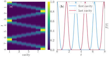
Figure 2: We consider an $N=8$ cavity only system with all $\Omega_{i}=0$ and $J_{i}$ couplings determined by Monte Carlo in 1, which converges to the values of the analytical solution. In panel (a) we graph the probability that the photon is in each cavity. The eight columns on the x axis represent the eight cavities, and time descends from 0 to 8 along the y axis. For every time and location, the probability is indicated in the color bar. In panel (b) we display the probabilities in just the originating and receiving cavities as functions of time. We observe perfect QST at time $\pi/2$ and with period $\pi$ for a return to the initial state.

III.2 QST in the Presence of Emitters

Next we demonstrate the effectiveness of our Monte Carlo solution of the IEP for determining cavity-cavity and cavity-emitter coupling leading to perfect QST in the novel context of the JCHH. Our method works only with systems with an even number of cavities when there is one emitter in every cavity. The reason is discussed further in the Appendix. However, with this constraint, we can successfully determine JCHH parameters giving fidelities ${\cal F}\gtrsim 0.99$ for systems with up to $N\sim 10^{\,2}$ cavities.

Perfect QST for a system of eight cavities with emitters in every cavity is shown in Fig. 3. Our labeling convention is such that we index of states with a photon in one of the $N=8$ optical cavities as 1-8, and states with the corresponding emitter in an excited level as 9-16. As with Fig. 2, the left panel is the heat map of the probability in all ‘sites’ (cavities and emitters), whereas the right panel focuses on the originating and receiving cavities only. We see that perfect QST is obtained in this ‘8+8’ JCHH system. However, the time evolution is considerably more complex than for the cavity-only (spin) system of Fig. 2. The transfer time remains $\pi/2$, but the peaks now form envelopes containing an additional higher frequency structure. This results from a rapid transfer of probability between each cavity and its associated emitter which occurs as the overall probability moves, with a longer time scale, down the cavity backbone.

Table 2 gives the values of the JCHH Hamiltonian parameters determined by our Monte Carlo and yielding the time evolution of Fig. 3. Values for $J_{i}$ and $g_{i}$ for several other $N$ are given in the Appendix, as is a discussion of an empirical formula which gives a reasonable fit to the data.

inter-cavity
bond $i$	$J_{i}\,$
1	4.521
2	6.158
3	7.232
4	7.979
5	7.232
6	6.158
7	4.521

cavity-emitter
bond $i$	$g_{i}\,$
1	9.558
2	7.825
3	5.872
4	3.234
5	3.234
6	5.872
7	7.825
8	9.558

Table 2: Values of the JCHH couplings determined by the Monte Carlo for an $N=8$ cavity array with an emitter in each cavity. Note that bond $J_{i}$ connects cavities $i$ and $i+1$ whereas bond $g_{i}$ connects cavity $i$ with its associated emitter. See Fig. 1.

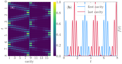
Figure 3: We consider a JCHH system of eight cavities and eight emitters with all $\Omega=\omega=0$ and couplings according to 2. Target eigenvalues were chosen to be those giving perfect QST for a $N=16$ cavity-only chain, i.e. using Eq. 4 with $N=16$. In panel (a) we graph the probability that the photon is in each cavity and in each emitter for multiple times. The sixteen columns on the x axis represent the eight cavities and eight emitters, and time descends from 0 to 8 along the y axis. For every time and location, the probability is indicated in the color bar. In panel (b) we display the probability in starting and receiving cavities as a function of time. We observe perfect QST at time $\pi/2$ and with period $\pi$.

IV Effect of Emitters on Perfect cavity-only QST

In the preceding section we demonstrated that perfect QST is possible for systems with uniform arrangements of emitters, precisely one per cavity. We now consider a distinct issue, namely what effect a single ‘impurity’ emitter would have on the perfect QST which would occur in a cavity-only system. This explores a different type of ‘disorder’ from that considered previously, and is experimentally relevant, since in cavity-emitter systems fluctuations in the numbers of emitters in each cavity are to be expected.

IV.1 Background: Limit of No Emitters

Again, we begin by establishing context for our new results on the effect of disorder in the JCHH by re-examining the cavity-only system previously considered in [9, 10] . We set $J_{0}=1$ as our scale of energy (time^-1) and add an ‘absolute’ random noise of scale $\Delta J=0.5$ to each of the engineered $J_{i}$ . We observe in Fig. 4 that, while we still see the oscillations present in the perfect system, the added noise significantly degrades QST.

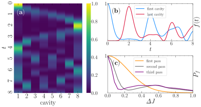
Figure 4: State transfer in a system of eight cavities with couplings according to Equation 4. A random disorder between $-\Delta J$ and $+\Delta J$ is added to each $J_{i}$. (a): Probability heat map for a single realization with $\Delta J=0.5$. (b): Associated fidelity line graph. We observe that perfect QST does not occur, and the fidelity in the last cavity decreases after each “pass.” (c): we graph the average fidelity for an $N=8$ cavity perfect QST system with varying levels of disorder $\Delta J$. The fidelity is measured at the expected transfer time $\frac{\pi}{2}$, and the average is taken over $10^{\,4}$ disorder realizations.

By calculating the fidelity at $t=\frac{\pi}{2}$ for many values of $\Delta J$ and taking the average fidelity over $10^{\,4}$ realizations of randomized disorder, we can determine the effect $\Delta J$ has on the fidelity. To emphasize the distinction from the fidelity for the clean system or for a single realization, we denote this average as ${\cal P}_{f}$. We obtain ${\cal P}_{f}$ for the first, second and third passes, where the $n$th pass is the fidelity taken at $t_{n}=\frac{\pi}{2}+(n-1)\cdot\pi$. The results are displayed in the bottom right panel of Fig. 4. The fidelity at the first pass decreases as the disorder increases, and in each successive pass the fidelity decreases more steeply. The second and third passes undergo a small rise after their initial declines, but this quickly flattens out. This non-monotonicity with $\Delta J$ is associated with the way in which the data are extracted: we measure $f(t)$ for each realization at the fixed clean system transfer time $t_{n}$. However $\Delta J$ not only disrupts the phase matching of the engineered $J_{i}$, it also alters the speed of propagation. An alternate (and computationally time-consuming) protocol would be to search over time for the optimal fidelity for each $\Delta J$ and for each realization.

We can also quantify the effects of random $\Omega_{i}$ by adding noise so that the cavity energy levels are uniformly distributed on $\big{(}-\frac{\Delta\Omega}{2},+\frac{\Delta\Omega}{2}\big{)}$. Such randomness can arise from variations in the size and shape of the cavities. Our observations (Fig. 5) are similar to our discussion of hopping disorder: We see oscillations with peaks that successively decline.

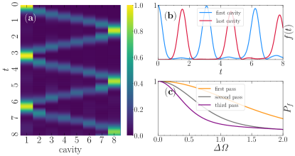
Figure 5: Analog of Fig. 4 except for disordered cavity energies rather than inter-cavity hopping. panels (a) and (b) give results for a single realization with $\Delta\Omega=1$, while panel (c) shows averages over many realizations for different $\Delta\Omega$. The fidelity loss appears to be roughly linear in the pass number for small $\Delta\Omega$; that is, the deviation in the maxima in the fidelity grow roughly linearly with $n$.

We now turn to analyzing the effects of adding atom-like emitters to our cavity-only system. We will first consider the effect of adding a single emitter to a cavity-only geometry with $J_{i}$ engineered to give perfect QST. We will next consider cases with many periodically placed, but non-uniform, emitters (random $g_{i}$ and $\omega_{i}$). The subsections below analyze these two situations.

IV.2 Loss of Fidelity due to Emitters

Figure 6 shows the first geometry we consider: a single emitter is added to a chain of $N$ cavities with couplings $J_{i}$. The position of the emitter is variable. The left panels of Fig. 7 describe the effects of such an impurity emitter on a cavity system with $J_{i}$ engineered to perfect QST. Results for different emitter cavity coupling $g$ and emitter placement are shown. An emitter at the edge of the chain (i.e. close to either the origin cavity or the destination cavity) causes the most rapid fidelity loss. It is interesting that the disruption of QST is less severe as the chain length increases (bottom left compared to top left). As with the independence of passage time on $N$, it is possible this greater robustness of perfect QST with $N$ is associated with the increasing values of $J_{i}$.

The right panels of Figure 7 consider another type of emitter disruption, namely a situation where an emitter is present in each cavity (all with the same $g_{i}=g$). The fidelity falls more rapidly with $g$ than for a single emitter (left panels), but there are periodic fidelity ‘revivals’ which are associated with the more regular geometric structure of uniform emitter placement.

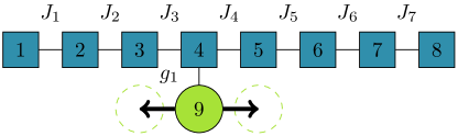
Figure 6: Geometry of the one dimensional (sparse) Jaynes-Cummings-Hubbard Hamiltonian with a single emitter. We will focus on the emitter’s effect on the fidelity for values of $J_{i}$ which give perfect QST for a cavity-only system.

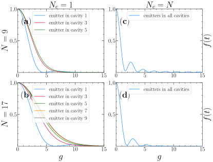
Figure 7: Effect of the addition of a single emitter as a perturbation to cavity-only perfect QST. (a): Fidelity $f(t=\pi/2)$ as a function of the coupling $g$ of the (single) ‘impurity’ emitter to its cavity. Curves for three emitter placements, cavities 1,3,5 are shown. (Reflection symmetry implies the effect of an emitter in cavity $N-i$ is identical to that of an emitter in cavity $i$.) The number of cavities $N=9$. (b): Same as (a) except for $N=17$. (c): Fidelity $f(t=\pi/2)$ as a function the coupling $g$ of a collection of emitters, one in each cavity, as a perturbation to cavity-only perfect QST. The number of cavities $N=9$. (d): Same as (c) except for $N=17$.

Finally, we examine disorder which has a similar form to randomness in $J_{i}$ considered in earlier spin-chain studies [9]. Specifically, we consider a situation of $N$ cavities, each with an emitter, but allow both the intercavity hoppings to be random on $(J_{i}-\frac{\Delta J}{2},J_{i}+\frac{\Delta J}{2})$, and the emitter-cavity couplings to be random on $(g_{i}-\frac{\Delta g}{2},g_{i}+\frac{\Delta g}{2})$, with $J_{i}$ and $g_{i}$ according to Table 2. The heat map of Fig. 8 gives the realization-averaged fidelity $P_{f}(\Delta g,\Delta J)$. The deterioration of perfect QST is more rapid here than in Fig. 7 because we not only have additional transfer paths provided by the emitters, but also these paths themselves have randomized hopping.

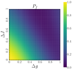
Figure 8: Fidelity $f(t=\pi/2)$ in the JCHH system of eight cavities and eight emitters as a function of varied cavity and emitter coupling disorder. The initial couplings are determined by the Monte Carlo procedure according to 2. For each realization, every coupling $J_{i}$ is randomly disordered between $J_{i}\pm\frac{\Delta J}{2}$. Similarly, each $g_{i}$ coupling is randomly disordered between $g_{i}\pm\frac{\Delta g}{2}$. Each data point is taken as the average fidelity over 200 realizations.

V The JCHH as a Realization of Boundary Engineering

This short section mainly makes an observation about an intriguing connection between ‘boundary engineering’ commonly discussed in spin chains [8] and cavity emitter systems. Topologically, and in the single excitation sector, a single emitter in an end cavity behaves identically to an additional cavity with $g$ playing the role of $J$. Thus there is a precise equivalence between the Hamitonian matrix and hence QST of systems with $N-2$ cavities and two ‘end’ emitters and ones with $N$ cavities and no emitters.

This mapping is especially interesting in that the known prescription for good QST when the $J_{i}$ are uniform except at the end requires $J_{1}$ and $J_{N}$ to be much less than the other, uniform $J_{i}$ in the chain interior. Such a situation arises very naturally in cavity-emitter systems. Hence this might be a promising alternate way to construct boundary engineered systems.

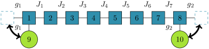
Figure 9: Geometry of the one dimensional Tavis-Cummings-Hubbard Hamiltonian with emitters only in the first and last cavities. The arrows indicate the geometric equivalence of this structure to a ‘boundary engineered’ spin chain for which only the first and last exchange constants $J_{1}=J_{7}=g$ are different from the bulk value $J$.

VI Multiple Excitations

Coupled cavity arrays differ from spin chains if more than one photon is present in the array, since two photons can occupy the same cavity, whereas an emitter can only be excited a single time. A final avenue of investigation described here concerns the case of multiple excitations in cavity-emitter systems. In the absence of emitters, perfect QST in the single excitation sector automatically implies perfect QST for multiple excitations: the photons are non-interacting particles. When emitters are present, this theorem no longer holds: emitters can only be excited once and hence the two excitation sector differs in a fundamental way from single excitation sector. Another way to phrase the non-triviality of multiple excitations is to note that even though the Hamiltonian is quadratic in the creation and destruction operators, usually a hallmark of the absence of interactions, the mixed nature of the allowed occupations introduces an effective ‘many-body’ correlation between excitations, in the sense that the eigen-energies of the two particle system are not sums of the single particle eigen-energies, as they would be if the character of the operators were purely bosonic or purely fermionic. Zhu etal have considered the contact interaction induced by the non-linearity of the JCHH in the context of the two-polariton scattering problem[35].

Figure 10 makes this observation more precise. The left panels are for a cavity only system with a single excitation at top, and two excitations at bottom. The same $\{\,J_{i}\,\}$ are used in the two cases. Perfect QST is preserved for multiple excitations[36]. The only difference is that the arrival time is more narrowly defined for two excitations.

On the other hand, in the two right panels, which are for a cavity-emitter system, perfect QST occurs in the case of a single excitation but is destroyed in the case of two excitations. As with the cavity-only geometry our procedure is to find the $\{\,J_{i},g_{i}\,\}$ which work for a single excitation (by targeting eigenvalues for a $2\,N$ cavity-only system as discussed earlier) and then simulate what happens for two excitations. We conclude that the ‘effective interaction’ induced by the mixed commutation rules introduces inter-particle scattering during the propagation.

A possible way to recover perfect QST for multiple excitations in the cavity-emitter case would be to use a different set of couplings for two excitations than for one. However, finding such a set is not straightforward. For single excitation systems, $N$ devices (cavities and emitters) will always have $N$ basis states, thus, given any given configuration of cavities and emitters, there exists a cavity only system with the same number of basis states. This means you can always tune these systems as you can create perfect QST systems with the same number of eigenvalues. This ceases to be the case for more than one excitation.

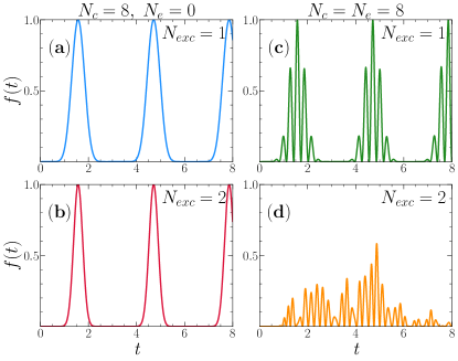
Figure 10: In the left column, the fidelity of a cavity-only system with a single excitation (top) and two excitations (bottom). The hoppings $\{\,J_{i}\,\}$ that give perfect QST for $N_{\rm exc}=1$ also do so for $N_{\rm exc}=2$, reflecting the non-interacting nature of the system. In the right column, similar data for the cavity-emitter system as shown in Fig. 1, with one excitation (top) and multiple excitations (bottom). For the cavity-emitter system, the JCHH parmeters $\{\,J_{i},g_{i}\,\}$ (determined by Monte Carlo) that give perfect QST for $N_{\rm exc}=1$ fail to give good fidelity for $N_{\rm exc}=2$. This is a consequence of the mixed bosonic/fermionic character of the JCHH operators which comes into play when $N_{\rm exc}>1$.

VII Experimental Parameters

We discuss here the typical range of values for the parameters in the JCHH which would arise in one of its potential realizations.

The proposed coupled cavity arrays with quantum emitters are well suited for implementations in color center platforms, such as silicon carbide and diamond. Color centers are quasi-atoms formed within the lattice defects of a semiconductor emitting at visible and near infra-red frequencies, 200 THz $<\omega/2\pi<$500 THz [37]. Recently, significant progress has been made in fabrication of optical cavities in these materials ($\Omega\approx\omega$) and the engineering of light and matter interaction with rates of $g/2\pi\sim$ 5 GHz [38]. This level of interaction, several orders of magnitude higher than achievable in atomic cavity QED systems, is a consequence of the large dipole momentum of color centers and the small mode volume of the cavities. It is worth noting that the optimal positioning of the color center, resulting in maximal $g$ value, is at the maximum of the electromagnetic field of the optical mode. An ensemble integrated into the cavity is likely to have a variation in individual emitter-cavity coupling rates. Scaling these systems into an array, photonic designs of coupled cavities have been proposed for a range of hopping rates 1 GHz $<J/2\pi<$ 200 GHz [22]. Variation of nanofabrication conditions across the sample may cause a variation in resonant frequencies of each cavity, however, methods such as photo-oxidation [39]. can be used to shift resonances and synchronize the system. Finally, intrinsic as well as fabrication-induced strain in the sample causes spectral disorder among color centers. This inhomogeneity has typically been in the $\sim$10 GHz range for a variety of emitters in silicon carbide and diamond [40, 21].

A link between fluctuations in $g_{i}$ and in emitter locations is that in a cavity with $M_{i}$ emitters there is a renormalization of the emitter-cavity coupling $g\rightarrow g\sqrt{M}$, or more specifically $\sqrt{\sum_{j=1}^{M}g_{j}^{2}}$) to form a polariton state. Thus fluctuations in $\{\,M_{i}\,\}$ serve as an additional source of randomness in $g_{i}$.

VIII Conclusions

Over the past two decades, the experimental realization of individual optical cavities, and their assembly into a CCA [41], has allowed for the study of a wealth of quantum many-body phenomena, including the simulation of strong correlation phenomena encountered in condensed matter physics [11, 42]. As with their ultracold atom, optical lattice counterparts [43, 44], cavity QED systems permit the manipulation of individual system components. This level of experimental control makes them attractive candidates for performing simulations of superfluid to Mott insulating behavior, Anderson localization, etc. When emitters are also present, new effects occur, including the emergence of polaritons, or quasiparticles consisting of a superposition of photonic and atomic excitations [45, 11, 46, 47]. The study of polaritons allows new strongly correlated regimes of light-matter interaction to be probed. Our study of quantum state transfer in such systems is complementary to those endeavors.

There are interesting analogies between the geometry considered here and that of the one dimensional Kondo or Periodic Anderson Hamiltonians. In those canons of condensed matter physics, electron hopping occurs between sites of a ‘conduction band’ (hence the analog of cavities here) while there are also ‘localized electrons’ which hybridize with their conduction electron partners but not each other (the analogs of emitters). The single particle physics of the periodic Anderson Hamiltonian is well understood: a hybridization gap opens where the flat impurity band crosses the conduction band. Our work directly connects to the QST problem in a one-dimensional, non-interacting, periodic Anderson Hamiltonian. It would be interesting to contrast the role of the ‘induced correlations’ in our cavity-emitter system which arise from mixed photon and emitter statistics, with the correlations arising from electron-electron interactions in the periodic Anderson Hamiltonian (which has only fermionic particles).

Acknowledgements J.M. and A.B. were supported by the Research Experience for Undergraduates program (NSF grant PHY-1852581). T.C. is a McNair and MURPPS scholar at the University of California, Davis. R.T.S. was supported by the grant DE‐SC0014671 funded by the U.S. Department of Energy, Office of Science. M.R. was supported by the National Science Foundation CAREER award 2047564.

IX Appendix

i. Constraint on parity of $N$ to solve the IEP

Our Monte Carlo solution to the IEP to determine $\{\,J_{i}\,\}$ and $\{\,g_{i}\,\}$ for $N$ cavities each with one emitter worked only for $N$ even. This is because for odd $N$ the parities of the number of cavities, $N$, and the number of cavities+emitters, $2N$, are different. More precisely, when $N$ is odd there is a zero eigenvalue in the spectrum of Eq. 4. We cannot reproduce this zero with our procedure of using the the cavity-only $2N$ spectrum as the target for the $N+N$ cavity-emitter spectrum.

To test this constraint on solvability further, we attempt a Monte Carlo solution for odd $N$, but removing the emitter in the central cavity, so that the number of cavities+emitters, $2N-1$ is now also odd. Results are given in Fig. 11 and demonstrate that (near) perfect QST is recovered.

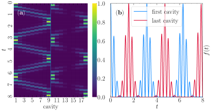
Figure 11: We consider a sparse JCHH system of nine cavities and eight emitters, in which all cavities except the center cavity contain an emitter. Target eigenvalues were chosen to be those giving perfect QST for a $N=17$ cavity-only chain. In panel (a) we graph the probability that the photon is in each cavity and in each emitter for multiple times. The eighteen columns on the x axis represent the nine cavities and eight emitters, with the center emitter column left as zero. Time descends from 0 to 8 along the y axis. For every time and location, the probability is indicated in the color bar. In panel (b) we display the probability in starting and receiving cavities as a function of time. We observe perfect QST at time $\pi/2$ and with period $\pi$.

	$N=N_{e}=12$		$N=N_{e}=16$
Bond $i$	$J_{i}$	$g_{i}$	$J_{i}$	$g_{i}$
1	5.597	14.755	6.519	19.929
2	7.712	13.056	9.030	18.264
3	9.255	11.278	10.876	16.511
4	10.322	9.261	12.310	14.708
5	11.355	7.025	13.515	12.753
6	12.007	3.987	14.461	10.581
7	11.355	3.987	15.294	8.0311
8	10.322	7.025	16.003	4.6159
9	9.255	9.261	15.294	4.6159
10	7.712	11.278	14.461	8.0311
11	5.597	13.056	13.515	10.581
12		14.755	12.310	12.753
13			10.876	14.708
14			9.0301	16.511
15			6.519	18.264
16				19.929

Table 3: Intercavity hoppings $J_{i}$ and cavity-emitter couplings $g_{i}$ which give perfect QST for $N=12$ and $N=16$ length cavity arrays with a single emitter in each cavity.

Bond $i$	$J_{i}\,$: MC	$J_{i}$: Eq. 7	$g_{i}\,$: MC	$g_{i}$: Eq. 8
1	4.521	4.527	9.558	9.562
2	6.158	6.164	7.824	7.806
3	7.232	7.246	5.872	5.826
4	7.979	8.000	3.234	3.231
5	7.232	7.246	3.234	3.231
6	6.158	6.164	5.872	5.826
7	4.521	4.527	7.824	7.806
8			9.558	9.562

Table 4: Comparison of the Monte Carlo (MC) and empirical cavity-cavity hoppings. We can see that the empirical formula, Eq. 7, for $J_{i}$ is extremely accurate to the Monte Carlo derived $J_{i}$, but the formula for $g_{i}$, Eq. 8, is less accurate. This may be because the actual form for $g_{i}$ is more complex than our current fitting form.

ii. Additional data for perfect QST in the JCHH

Since a primary result of this paper is the computation of $\{\,J_{i},g_{i}\,\}$ which result in perfect QST for cavity-emitter systems, described by the JCHH, we provide in Table 3 some additional results for large size systems, $N=12,16$ to complement the $N=8$ data provided in the main text.

iii. Functional form for perfect QST JCHH couplings

In the case of the cavity-only (spin chain), precise formulae for the intercavity-hopping (Heisenberg exchange) constants to achieve perfect QST are known. The earliest example is that of Christandl and given by Eq. 4. In the main manuscript we described a Monte Carlo process which works in the more general cavity-emitter geometry. However, this solution is a ‘black box’ in the sense that it produces raw numbers which achieve (near) perfect QST without providing analytic insight or a formula.

We have attempted to fit the raw data produced by the simulation to simple functional forms. We mimic the spin-chain solution [2] with an ansatz of the square root of a polynomial function on $N$ and $i$. Indeed, the data collected allows a good fit to the empirical formulae:

$$J_{i}=\frac{\sqrt{i(11N-6i)}}{2}$$ (7)

$$g_{i}=\frac{\sqrt{(2i-N-1)(14i-27N-7)}}{4}$$ (8)

Table 4 compares the Monte Carlo values with these empirical formulae.

iv. Criterion for perfect QST

We note that it is non-trivial to distinguish whether small deviations from fidelity ${\cal F}\equiv 1$ arise from a fundamental inability to achieve perfect QST or from small randomness in the Monte Carlo evaluation of the couplings. We use the term ‘perfect QST’ when our numerics indicate that by systematically running longer we can achieve arbitrarily close to ${\cal F}\equiv 1$. In principle an extrapolation of ${\cal F}$ as a function of simulation time would provide a more rigorous analysis. We do not do this here, because such an extrapolation is complicated by the necessity to tune the annealing protocol, i.e. the manner in which $\beta$ is increased, as well as the choices for the initial $\beta_{i}$ and final $\beta_{f}$. We therefore elect to use a more loose definition of ‘perfect QST’, ${\cal F}$ very close to 1 and systematically improvable.

References

- Bose [2003] S. Bose, Quantum communication through an unmodulated spin chain, Physical Review Letters 91, 207901 (2003).
- Christandl et al. [2004] M. Christandl, N. Datta, A. Ekert, and A. J. Landahl, Perfect state transfer in quantum spin networks, Physical Review Letters 92, 187902 (2004).
- Christandl et al. [2005] M. Christandl, N. Datta, T. C. Dorlas, A. Ekert, A. Kay, and A. J. Landahl, Perfect transfer of arbitrary states in quantum spin networks, Physical Review A 71, 032312 (2005).
- Karbach and Stolze [2005] P. Karbach and J. Stolze, Spin chains as perfect quantum state mirrors, Physical Review A 72, 030301 (2005).
- Bose [2007] S. Bose, Quantum communication through spin chain dynamics: an introductory overview, Contemporary Physics 48, 13 (2007).
- Felicetti et al. [2014] S. Felicetti, G. Romero, D. Rossini, R. Fazio, and E. Solano, Photon transfer in ultrastrongly coupled three-cavity arrays, Physical Review A 89, 013853 (2014).
- Almeida et al. [2016a] G. M. Almeida, F. Ciccarello, T. J. Apollaro, and A. M. Souza, Quantum-state transfer in staggered coupled-cavity arrays, Physical Review A 93, 032310 (2016a).
- Banchi [2013] L. Banchi, Ballistic quantum state transfer in spin chains: General theory for quasi-free models and arbitrary initial states, The European Physical Journal Plus 128, 1 (2013).
- Zwick et al. [2011] A. Zwick, G. A. Álvarez, J. Stolze, and O. Osenda, Robustness of spin-coupling distributions for perfect quantum state transfer, Physical Review A 84, 022311 (2011).
- Zwick et al. [2015] A. Zwick, G. A. Álvarez, J. Stolze, and O. Osenda, Quantum state transfer in disordered spin chains: How much engineering is reasonable?, Quant. Inf. Comput. 15, 582 (2015).
- Hartmann et al. [2008] M. J. Hartmann, F. G. Brandao, and M. B. Plenio, Quantum many-body phenomena in coupled cavity arrays, Laser & Photonics Reviews 2, 527 (2008).
- Angelakis et al. [2007] D. G. Angelakis, M. F. Santos, and S. Bose, Photon-blockade-induced Mott transitions and XY spin models in coupled cavity arrays, Physical Review A 76, 031805 (2007).
- Tomadin and Fazio [2010] A. Tomadin and R. Fazio, Many-body phenomena in QED-cavity arrays, JOSA B 27, A130 (2010).
- Hartmann [2016] M. J. Hartmann, Quantum simulation with interacting photons, Journal of Optics 18, 104005 (2016).
- Majumdar et al. [2012] A. Majumdar, A. Rundquist, M. Bajcsy, V. D. Dasika, S. R. Bank, and J. Vučković, Design and analysis of photonic crystal coupled cavity arrays for quantum simulation, Physical Review B 86, 195312 (2012).
- Radulaski [2017] M. Radulaski, Silicon Carbide and Color Center Quantum Photonics, Ph.D. thesis, Stanford University (2017).
- Koehl et al. [2011] W. F. Koehl, B. B. Buckley, F. J. Heremans, G. Calusine, and D. D. Awschalom, Room temperature coherent control of defect spin qubits in silicon carbide, Nature 479, 84 (2011).
- Widmann et al. [2015] M. Widmann, S.-Y. Lee, T. Rendler, N. T. Son, H. Fedder, S. Paik, L.-P. Yang, N. Zhao, S. Yang, I. Booker, et al., Coherent control of single spins in silicon carbide at room temperature, Nature materials 14, 164 (2015).
- Lukin et al. [2020] D. M. Lukin, C. Dory, M. A. Guidry, K. Y. Yang, S. D. Mishra, R. Trivedi, M. Radulaski, S. Sun, D. Vercruysse, G. H. Ahn, et al., 4H-silicon-carbide-on-insulator for integrated quantum and nonlinear photonics, Nature Photonics 14, 330 (2020).
- Radulaski et al. [2017] M. Radulaski, M. Widmann, M. Niethammer, J. L. Zhang, S.-Y. Lee, T. Rendler, K. G. Lagoudakis, N. T. Son, E. Janzen, T. Ohshima, et al., Scalable quantum photonics with single color centers in silicon carbide, Nano letters 17, 1782 (2017).
- Babin et al. [2021] C. Babin, R. Stöhr, N. Morioka, T. Linkewitz, T. Steidl, R. Wörnle, D. Liu, E. Hesselmeier, V. Vorobyov, A. Denisenko, et al., Fabrication and nanophotonic waveguide integration of silicon carbide colour centres with preserved spin-optical coherence, Nature Materials 10.1038, s41563 (2021).
- Majety et al. [2021] S. Majety, V. Norman, L. Li, M. Bell, P. Saha, and M. Radulaski, Quantum photonics in triangular-cross-section nanodevices in silicon carbide, Journal of Physics: Photonics 3, 034008 (2021).
- Hepp et al. [2014] C. Hepp, T. Müller, V. Waselowski, J. N. Becker, B. Pingault, H. Sternschulte, D. Steinmüller-Nethl, A. Gali, J. R. Maze, M. Atatüre, et al., Electronic structure of the silicon vacancy color center in diamond, Physical Review Letters 112, 036405 (2014).
- Sipahigil et al. [2014] A. Sipahigil, K. D. Jahnke, L. J. Rogers, T. Teraji, J. Isoya, A. S. Zibrov, F. Jelezko, and M. D. Lukin, Indistinguishable photons from separated silicon-vacancy centers in diamond, Physical review letters 113, 113602 (2014).
- Zhang et al. [2018] J. L. Zhang, S. Sun, M. J. Burek, C. Dory, Y.-K. Tzeng, K. A. Fischer, Y. Kelaita, K. G. Lagoudakis, M. Radulaski, Z.-X. Shen, et al., Strongly cavity-enhanced spontaneous emission from silicon-vacancy centers in diamond, Nano letters 18, 1360 (2018).
- Bradac et al. [2019] C. Bradac, W. Gao, J. Forneris, M. E. Trusheim, and I. Aharonovich, Quantum nanophotonics with group IV defects in diamond, Nature communications 10, 1 (2019).
- Yung and Bose [2005] M.-H. Yung and S. Bose, Perfect state transfer, effective gates, and entanglement generation in engineered bosonic and fermionic networks, Physical Review A 71, 032310 (2005).
- Note [1] In statistical mechanics language is the inverse temperature, so that corresponds to high temperature and corresponds to low temperature. The gradual increase of (lowering of ) allows the Monte Carlo to find the ‘ground state’ where the and give a Hamiltonian with desired target eigenvalues to high accuracy.
- Note [2] An alternate Monte Carlo procedure defines an action based on targeting of a desired time evolution matrix rather than desired eigenvalues. This procedure is useful in more complicated geometries and will be explored in a subsequent paper.
- Note [3] In future work we will explore yet more general geometries.
- Chu et al. [2005] M. Chu, M. T. Chu, and G. Golub, Inverse eigenvalue problems: theory, algorithms, and applications, Vol. 13 (Oxford University Press, 2005).
- Hald [1976] O. H. Hald, Inverse eigenvalue problems for jacobi matrices, Linear Algebra and Its Applications 14, 63 (1976).
- Chu and Golub [2002] M. T. Chu and G. H. Golub, Structured inverse eigenvalue problems, Acta Numerica 11, 1 (2002).
- Note [4] Situations where the randomness is ‘relative’, i.e. scaled to the on each site, have also been studied [10].
- Zhu et al. [2013] C.-Z. Zhu, S. Endo, P. Naidon, and P. Zhang, Scattering and bound states of two polaritons in an array of coupled cavities, Few-Body Systems 54, 1921 (2013).
- Perez-Leija et al. [2013] A. Perez-Leija, R. Keil, H. Moya-Cessa, A. Szameit, and D. N. Christodoulides, Perfect transfer of path-entangled photons in photonic lattices, Phys. Rev. A 87, 022303 (2013).
- Norman et al. [2021] V. A. Norman, S. Majety, Z. Wang, W. H. Casey, N. Curro, and M. Radulaski, Novel color center platforms enabling fundamental scientific discovery, InfoMat 3, 869 (2021).
- Evans et al. [2018] R. E. Evans, M. K. Bhaskar, D. D. Sukachev, C. T. Nguyen, A. Sipahigil, M. J. Burek, B. Machielse, G. H. Zhang, A. S. Zibrov, E. Bielejec, H. Park, M. Lončar, and M. D. Lukin, Photon-mediated interactions between quantum emitters in a diamond nanocavity, Science 362, 662 (2018).
- Piggott et al. [2014] A. Y. Piggott, K. G. Lagoudakis, T. Sarmiento, M. Bajcsy, G. Shambat, and J. Vučković, Photo-oxidative tuning of individual and coupled GaAs photonic crystal cavities, Opt. Express 22, 15017 (2014).
- Schröder et al. [2017] T. Schröder, M. E. Trusheim, M. Walsh, L. Li, J. Zheng, M. Schukraft, A. Sipahigil, R. E. Evans, D. D. Sukachev, C. T. Nguyen, J. L. Pacheco, R. M. Camacho, E. S. Bielejec, M. D. Lukin, and D. Englund, Scalable focused ion beam creation of nearly lifetime-limited single quantum emitters in diamond nanostructures, Nature Communications 8, 15376 (2017).
- Saxena et al. [2021] A. Saxena, Y. Chen, Z. Fang, and A. Majumdar, Photonic topological baths for quantum simulation, arXiv preprint arXiv:2106.14325 (2021).
- Smith et al. [2021] K. C. Smith, A. Bhattacharya, and D. J. Masiello, Exact -body representation of the jaynes-cummings interaction in the dressed basis: Insight into many-body phenomena with light, arXiv preprint arXiv:2103.07571 (2021).
- Schäfer et al. [2020] F. Schäfer, T. Fukuhara, S. Sugawa, Y. Takasu, and Y. Takahashi, Tools for quantum simulation with ultracold atoms in optical lattices, Nature Reviews Physics 2, 411 (2020).
- Esslinger [2010] T. Esslinger, Fermi-Hubbard physics with atoms in an optical lattice, Annu. Rev. Condens. Matter Phys. 1, 129 (2010).
- Bose et al. [2007] S. Bose, D. G. Angelakis, and D. Burgarth, Transfer of a polaritonic qubit through a coupled cavity array, Journal of Modern Optics 54, 2307 (2007).
- Almeida et al. [2016b] G. M. Almeida, F. Ciccarello, T. J. Apollaro, and A. M. Souza, Quantum-state transfer in staggered coupled-cavity arrays, Physical Review A 93, 032310 (2016b).
- Hartmann et al. [2006] M. J. Hartmann, F. G. Brandao, and M. B. Plenio, Strongly interacting polaritons in coupled arrays of cavities, Nature Physics 2, 849 (2006).