Quantum Architecture Search via Continual Reinforcement Learning

Abstract

Quantum computing has promised significant improvement in solving difficult computational tasks over classical computers. Designing quantum circuits for practical use, however, is not a trivial objective and requires expert-level knowledge. To aid this endeavor, this paper proposes a machine learning-based method to construct quantum circuit architectures. Previous works have demonstrated that classical deep reinforcement learning (DRL) algorithms can successfully construct quantum circuit architectures without encoded physics knowledge. However, these DRL-based works are not generalizable to settings with changing device noises, thus requiring considerable amounts of training resources to keep the RL models up-to-date. With this in mind, we incorporated continual learning to enhance the performance of our algorithm. In this paper, we present the Probabilistic Policy Reuse with deep Q-learning (PPR-DQL) framework to tackle this circuit design challenge. By conducting numerical simulations over various noise patterns, we demonstrate that the RL agent with PPR was able to find the quantum gate sequence to generate the two-qubit Bell state faster than the agent that was trained from scratch. The proposed framework is general and can be applied to other quantum gate synthesis or control problems– including the automatic calibration of quantum devices.

I Introduction

Since the conception of quantum computing (QC) feynman1985quantum , many researchers and engineers have sought to use it to solve problems which cannot be practically solved by a classical computer. Theoretically, quantum computing has promised exponential or quadratic speedups for several difficult computational problems that are otherwise intractable on a classical computer harrow2017quantum ; arute2019quantum ; nielsen2002quantum , such as: factorizing large integers shor1999polynomial and unstructured database searches grover1997quantum . In practice, the applications of QC are largely limited by the capabilities of existing noisy quantum devices preskill2018quantum which do not have fidelity-preserving measures such as quantum error correction nielsen2002quantum ; gottesman1997stabilizer ; gottesman1998theory and thus cannot carry out sophisticated quantum computational tasks faithfully. Variational quantum algorithms (VQA) have been one approach to dealing with these Noisy Intermediate Scale Quantum (NISQ) devices. Recent developments in VQA provide a framework to design near-term quantum applications in various scenarios cerezo2020variational ; bharti2021noisy . VQA-based applications include solving quantum chemistry problems peruzzo2014variational as well as machine learning (ML) tasks such as: function approximation chen2020quantum ; mitarai2018quantum ; paine2021quantum ; kyriienko2021solving , classification mitarai2018quantum ; schuld2018circuit ; havlivcek2019supervised ; Farhi2018ClassificationProcessors ; benedetti2019parameterized ; mari2019transfer ; abohashima2020classification ; easom2020towards ; sarma2019quantum ; stein2020hybrid ; chen2020hybrid ; chen2020qcnn ; wu2020application ; stein2021quclassi ; chen2021hybrid ; jaderberg2021quantum ; mattern2021variational ; hur2021quantum ; li2021recent , generative modeling dallaire2018quantum ; stein2020qugan ; zoufal2019quantum ; situ2018quantum ; nakaji2020quantum , deep reinforcement learning chen19 ; lockwood2020reinforcement ; jerbi2019quantum ; Chih-ChiehCHEN2020 ; wu2020quantum ; skolik2021quantum ; jerbi2021variational ; kwak2021introduction ; nagy2021photonic ; chen2021variational , sequence modeling chen2020quantum ; bausch2020recurrent ; takaki2020learning ; abbaszade2021application , speech recognition yang2020decentralizing , metric and embedding learning lloyd2020quantum ; nghiem2020unified , transfer learning mari2019transfer and federated learning chen2021federated ; yang2020decentralizing ; chehimi2021quantum . Despite these achievements, it is still a non-trivial task to design a good quantum circuit architecture for specific computational tasks and such difficulties may hinder a wider acceptance of QC.

Concurrently, many advancements have been made in applying classical computing techniques to solve complex tasks. The most prominent example is the significant progress in machine learning (ML) and artificial intelligence (AI) methodologies. Modern deep neural network (DNN)-based models lecun2015deep ; goodfellow2016deep , which utilize the principles of deep learning (DL), have been applied to a diverse set of areas and have been shown to be highly successful in: computer vision voulodimos2018deep ; simonyan2014very ; lecun1998gradient , natural language processing bahdanau2014neural ; vaswani2017attention ; young2018recent ; otter2020survey , and playing the game of Go or many video games with superhuman performance mnih2015human ; silver2017mastering ; silver2016mastering ; schrittwieser2019mastering ; badia2020agent57 , just to name a few. Among these, deep reinforcement learning (DRL) is of our particular interest, as it is designed to solve highly sophisticated sequential decision making tasks sutton2018reinforcement ; bertsekas2021rollout .

With powerful RL techniques in hand, it is natural to explore the potential application of RL to address several long-standing problems in quantum computing– especially the ones which can be reformulated into a sequential decision problem. Recent research has employed the extraordinary capabilities of RL to tackle several challenges in quantum computing such as quantum error correction (QEC) nautrup2019optimizing ; andreasson2019quantum ; colomer2020reinforcement ; sweke2020reinforcement and quantum control niu2019universal ; an2019deep ; bukov2018reinforcement ; fosel2018reinforcement ; zhang2019does ; palittapongarnpim2017learning ; xu2019generalizable ; brown2021reinforcement ; baum2021experimental . The common feature among these QC applications is that these tasks can be framed as sequential decision problems. For example, in QEC the goal is to design gate sequences to either encode or decode the quantum states. In the context of the quantum control problem, specific hardware operation sequences (e.g. pulse sequences) are generated to synthesize a desired quantum state or a quantum gate functionality. Another QC problem which can be thought of in this manner is to find a quantum gate sequence in order to achieve a certain computing task. This is called a quantum architecture search problem and is the task we are focusing on in this paper.

The goal of a quantum architecture search (QAS) algorithm is to find a proper quantum circuit or gate sequence which can be used to achieve a specific quantum computational task. Ideally, the generated circuit architecture should use as few operations as possible to minimize the effect of device noises. Additionally, the QAS algorithm should be hardware-aware, meaning that the algorithm should be able to provide circuit architectures tailored for the specific quantum hardware available. An important distinction is that the QAS problem is different from the quantum control problem baum2021experimental , since the latter focuses on generating control pulses on the hardware level baum2021experimental . We are interested in QAS algorithms since they can be used in the workflow of quantum compilation, a procedure to transfer quantum algorithms into a gate sequence suitable for a particular quantum device.

The QAS problem has taken inspiration from classical ML techniques and challenges. In classical ML, especially in deep learning, although the models can perform certain tasks pretty well, they are also extremely complex he2016deep and contain many components which require manual tuning. Numerous efforts have been made to build automatic procedures to generate well-performing deep neural network architectures for given tasks zoph2016neural ; baker2016designing ; cai2017efficient ; zoph2018learning ; zhong2018practical ; schrimpf2017flexible ; pham2018efficient ; cai2018path ; elsken2019neural , which is known as a neural architecture search (NAS). A common method for NAS is to use RL to sequentially generate or place neural network blocks zoph2016neural ; baker2016designing . It has been shown that various RL-based methods can generate neural architectures that can achieve performance superior than manually-crafted ones zoph2016neural ; baker2016designing . Such achievements led to the exploration of RL-based methods in QAS and recently, researchers have started to apply RL for certain kinds of QAS tasks ostaszewski2021reinforcement ; fosel2021quantum ; pirhooshyaran2020quantum ; bolens2021reinforcement .

Despite RL being a powerful solution to sequential decision making problems, it still has its drawbacks– a significant issue that the RL framework faces is the need to retrain the agent whenever the environment changes. In the context of hardware-aware QAS, the drifting device noise patterns may reduce the effectiveness of RL-based results. This re-acquisition of information is extremely inefficient due to its redundancy and is precisely the problem we target in this paper.

In this paper, we implement a continual learning scheme to allow the RL agent to learn how to generate quantum circuit architectures in fewer learning episodes when placed in different environments of varying noise-levels. To account for the inefficiency of retraining the agent when the noise pattern is different, we implement an additional aspect of continual learning to our scheme such that the agent will be able to store and reuse the information or policies it learned from previous training environments. Concretely, the learned policies will form a policy library for future use. When the agent encounters a new environment, the past policies from the library will serve as the a priori conditions for the exploration. Instead of exploring the completely random actions, the past policies can be a reasonable foundation for building new policies for an unseen environment. We demonstrate via numerical simulations that such intuitive construction, though very simple conceptually, can largely boost the training efficiency of these quantum architecture searching RL agents.

Our contributions are the following:

• We provide a framework to study how continual reinforcement learning can be applied to quantum architecture search problems.

• We demonstrate building a quantum circuit step-by-step via continual reinforcement learning methods, which allows for new policies to be formed from policies acquired in previous training environments with varying noise levels.

The paper is organized as follows. In Section II we introduce the quantum architecture search (QAS) problem that our agent will solve. In Section III, we introduce the RL background knowledge used in this work. In Section IV, we introduce the idea of continual learning which will be used to increase the capabilities of existing DQN when dealing with changing environments. In Section V, we describe the proposed continual DQN used for the QAS. In Section VI, we describe the details of our experimental methodology and our hyperparameter settings. In Section VII, we present the numerical simulation results of the continual DQN as well as the results of the DQN without continual learning for comparison. Finally we discuss the results in Section VIII and offer concluding remarks in Section IX.

II Quantum Architecture Search (QAS) Problem

Quantum architecture search (QAS) is an algorithmic procedure designed to find a series of quantum operations or quantum gates to achieve a predefined target such as generating the desired quantum state from an initial state. Concretely, given an initial state $\ket{0\cdots 0}$ and the target state $\ket{\Psi}$, the goal is to find out a proper quantum gate sequence such that after the operation of these gates, the initial state can be transformed into the target state within a certain error tolerance. We will be using RL to achieve this goal. In the context of RL training, the environment $\mathcal{E}$ is the quantum computer or quantum simulator. In this work, we chose to use a quantum simulator (the details of which can be found in Section VI). In using the quantum simulator, we can define various noise or error pattern to evaluate and test the capability of our proposed continual RL framework. Another reason for using a quantum simulator over a real quantum computer is that it is currently impractical to directly train a large number of episode through cloud-based quantum platforms.

The observations, used by the RL agent to process the state of the system, are composed of several Pauli measurements (e.g. Pauli-$X$, $Y$ and $Z$ expectation values from each qubit) and the agent calculates a reward value from the fidelity (similarity) of the generated state to the target state. In each time-step, the RL agent chooses an action $a$ from the action set $\mathcal{A}$, which includes various quantum gates (one- and two-qubit gates) and the index of the qubit they will operate on. The agent updates the quantum circuit with the selected action and then the environment $\mathcal{E}$ executes the new circuit and calculates the fidelity of the current state to the target state. If the fidelity is greater than a predefined value– meaning that the quantum state is within an accepted error tolerance to the target state– then the episode ends there and a large positive reward is fed back to the agent. If, however, the fidelity is below the predefined value, the RL agent will be penalized with a small negative reward before moving onto the next time-step. During each time-step, the environment $\mathcal{E}$ returns Pauli expectation values of each qubit as the observations (or states), to the RL agent. For an $n$-qubit system, the dimension of the state or observation vector is subsequently $3n$. The procedure continues until the RL agent reaches either a sufficiently high value of fidelity or the maximum allowed steps. Various algorithmic procedures such as the policy gradient method or deep Q-learning can be used to optimize the RL agent.

For example, the previous work kuo2021quantum has demonstrated that DRL algorithms were able to sample from a set of basic quantum gates in order to incrementally construct a quantum gate sequence that yielded a desired output state. This capability was seen in quantum circuit architectures consisting of two- and three-qubits and the target state of that paper was the Bell state (two-qubit) and the GHZ state (three-qubit). Conceptually, the Bell state and GHZ state are equivalent states for systems with different numbers of qubits. This state was picked due to it’s prominent usage in quantum computing and quantum communication for the purpose of quantum entanglement.

Although the DRL algorithms in the previous paper kuo2021quantum were successful, there is critical limitation to that framework. The requirement to retrain the RL agent for each new task (such as environments of varying noise levels) reduces the usefulness of the method in quantum device calibration. In order to address this obstacle, we incorporated a continual learning framework (described in the Section IV and Section V) to the DRL training procedure such that the RL agent can leverage previously gained knowledge when encountering a new environment.

In this paper, we retained the Bell state as our target state, and adopted a similar assessment (reward) scheme as before kuo2021quantum to now evaluate the continual DRL algorithm which uses probabilistic policy reuse. The Bell state has the following circuit solution for a two-qubit system:

@C=1em @R=1em —0⟩ & H 1

—0⟩

Figure 1: Quantum circuit for the Bell state.

Figure 1 shows the optimal circuit solution which the RL agent will be trying to construct incrementally in environments with different noise-conditions.

III Reinforcement Learning

Reinforcement learning (RL) is a method of machine learning which allows the agent to learn by optimizing a score based on its interactions with the environment  sutton2018reinforcement . The agent interacts with an environment $\mathcal{E}$ over a number of discrete time steps. At each time step $t$, the agent receives a observation or state $s_{t}$ from the environment $\mathcal{E}$ and feeds that information into its current policy $\pi$ in order to choose an action $a_{t}$ from a set of possible actions $\mathcal{A}$. The policy $\pi$ is a function which maps the state or observation $s_{t}$ to an action $a_{t}$. In general, the policy can be stochastic– for a given state $s$, the action output can be a probability distribution $\pi(a_{t}|s_{t})$ conditioned on $s_{t}$. After executing the action $a_{t}$, the agent receives the state of the next time step $s_{t+1}$ and based on that state it gets a scalar reward $r_{t}$. This reward is what affects the score of the agent for this task. It can either be a positive quantity (which indicates that a good move was made) or a negative quantity (which can be thought of as a penalty/deduction for a bad choice). This process is continued until the agent reaches the terminal state or a pre-defined stopping criteria (e.g. the maximum steps allowed). An episode is defined as an agent starting from a randomly selected initial state and following the aforementioned process either all the way through until it gets to the terminal state or until it reaches the stopping criteria.

We define the total discounted return from time step $t$ as $R_{t}=\sum_{t^{\prime}=t}^{T}\gamma^{t^{\prime}-t}r_{t^{\prime}}$, where $\gamma$ is a discount factor in $(0,1]$. The role of $\gamma$ is have a parameter to control how future rewards are weighted to the decision making function. When a large $\gamma$ is considered, the agent weighs the future reward more heavily. On the other hand, with a small $\gamma$, future rewards are quickly ignored and immediate reward will be weighted more. The value of $\gamma$ can vary across time steps as well and this is what was done in this paper (Section VI). The goal of the agent is to maximize the expected return from each state $s_{t}$. The action-value function or Q-value function $Q^{\pi}(s,a)=\mathbb{E}[R_{t}|s_{t}=s,a]$ is the expected return for selecting an action $a$ in state $s$ based on policy $\pi$. The optimal action value function $Q^{*}(s,a)=\max_{\pi}Q^{\pi}(s,a)$ will give the maximal action-value across all possible policies. The agent’s expected return from following policy $\pi$ at state $s$ is given by $V^{\pi}(s)=\mathbb{E}\left[R_{t}|s_{t}=s\right]$, which is called a value function. There are various RL algorithms which are designed to find the policy that maximizes the value function. This framework of using RL algorithms to maximize the value function is called value-based RL.

III.1 Q-Learning

Q-learning sutton2018reinforcement is a model-free approach to the RL algorithm, meaning it does not attempt to learn about the underlying transition dynamics. Before the learning process begins, the value function $Q$ is randomly initialized. Then, at each time step $t$, the agent selects an action $a_{t}$ (using a selection function such as an $\epsilon$-greedy policy derived from $Q$). The agent then observes the reward $r_{t}$ that resulted from this action and enters a new state $s_{t+1}$. After the agent enters the new state $s_{t+1}$, $Q$ is updated with the learning rate $\alpha$. This makes Q-learning an off-policy learning technique since it updates its Q-values using the observed reward $r_{t}$ and the maximum reward $\max_{a}Q\left(s_{t+1},a\right)$ of the next state $s_{t+1}$ over all possible actions $a$. The updating is done according to the following benchmark formula:

$$Q\left(s_{t},a_{t}\right)\leftarrow Q\left(s_{t},a_{t}\right)+\alpha\left[r_{t}+\gamma\max_{a}Q\left(s_{t+1},a\right)-Q\left(s_{t},a_{t}\right)\right].$$ (1)

III.2 Deep Q-Learning

The action-value function $Q(s,a)$ can be represented by a two-dimensional table with $s\times a$ total entries, that is, the number of possible states times the number of possible actions. However, when the state space or the action space $\mathcal{A}$ is large or even continuous, the tabular method is unfeasible. In these situations, the action-value function can be represented with function approximators such as neural networks mnih2016asynchronous ; mnih2015human . This neural-networks-based reinforcement learning is called deep reinforcement learning (DRL).

The usage of neural networks as function approximators in order to represent the $Q$-value function has been studied extensively mnih2016asynchronous ; mnih2015human and has been shown to be successful in many tasks such as playing video games. In this setting, the action-value function $Q(s,a;\theta)$ is parameterized by $\theta$, which can be derived using a series of iterations from a variety of optimization methods adopted from other machine learning tasks. The simplest form of DRL is deep Q-learning. For deep Q-learning, the goal is to directly approximate the optimal action-value function $Q^{*}(s,a)$ by minimizing the mean square error (MSE) loss function:

$$L(\theta)=\mathbb{E}[(r_{t}+\gamma\max_{a^{\prime}}Q(s_{t+1},a^{\prime};\theta^{-})-Q(s_{t},a_{t};\theta))^{2}].$$ (2)

Here, the prediction is $Q(s_{t},a_{t};\theta)$, where $\theta$ is the parameter of a policy network (the network from which we extract our solution) and the target is $r_{t}+\gamma\max_{a^{\prime}}Q(s_{t+1},a^{\prime};\theta^{-})$, where $\theta^{-}$ is the parameter of the target network (created to help stabilize the optimization procedure) and $s_{t+1}$ is the state encountered after performing action $a_{t}$ at state $s_{t}$.

In DRL, it is ideal for the loss function to converge but oftentimes it is very difficult to get it to do so. In fact, the loss function will usually be divergent when a nonlinear approximator like a neural network is used to represent the action-value function mnih2015human . There are several possible reasons for why this happens. When the states or observations are serially correlated along the temporal trajectory –thereby violating the assumption that the samples are independent and identically distributed (IID)– the $Q$ function varies dramatically and subesquently changes the policy at a relatively large scale. Besides the states being correlated, another reason for divergence could be due to having a large correlation between the action-value $Q$ and the target values $r_{t}+\gamma\max_{a^{\prime}}Q(s_{t+1},a^{\prime})$. Unlike in supervised learning where the targets are given and invariant, the settings of DRL allow targets to vary with $Q(s,a)$, causing $Q(s,a)$ to chase a nonstationary target.

The deep Q-learning (DQL) or deep Q-network (DQN) presented in the work mnih2015human addressed these issues by implementing two mechanisms:

• Experience replay: To perform experience replay, one stores each transition the agent encounters a tuple in the following form: $(s_{t},a_{t},r_{t},s_{t+1})$ for each time step $t$. To update the $Q$-learning parameters, one randomly samples a batch of experiences from the replay memory and then performs gradient descent with the following MSE loss function: $L(\theta)=\operatorname*{\mathbb{E}}[(r_{t}+\gamma\max_{a^{\prime}}Q(s_{t+1},a^{\prime};\theta^{-})-Q(s_{t},a_{t};\theta))^{2}]$, where the loss function is calculated over the previously sampled batch from the replay memory. The key feature of adding the experience replay is to lower the correlation of the inputs for training the $Q$-function.

• Target Network: Here $\theta^{-}$ is the parameter of the target network and these parameters are only updated after a certain number of finite time steps. This setting helps to stabilize the $Q$-value function training since the target is relatively stationary compared to the action-value function.

In the next section, we will introduce the proposed continual DQN which is capable of reusing previous policies. The major components of DQN such as experience replay and target network will be preserved.

With DRL, the agent is encouraged to move towards the optimal solution over time while considering previous actions. The DRL agent associates its performance with the score it receives every learning episode and aims to improve upon that score as episodes progress. From the system that was carried over from the previous paper kuo2021quantum , the scores in these experiments are calculated by taking the quantum state fidelity (in other words, how close the observed output state was to our target Bell state) and subtracting the penalty term (0.01) for each step taken. This can be seen in the following equation (Equation 3):

$$Episode\ Score=State\ Fidelity-(0.01)\cdot(number\ of\ steps\ taken)$$ (3)

Having a higher episode score meant that the quantum state is close to the Bell state (high state fidelity) and that not many gates were used in the circuit construction (small number of steps).

IV Continual Learning

Recent advances in deep RL have reached several extraordinary achievements through beating their best human competitors on a variety of challenging tasks mnih2015human ; silver2016mastering ; silver2017mastering . However, within existing approaches, a computational agent is trained to master a narrow task of interest. Moreover, untrained computational agents require significantly more training episodes to reach a good performance compared to their human competitors. After training, it is hard to be generalized to other similar tasks, even simple RL ones bengio2020interference . In contrast, humans have the capability to continually learn new skills and incrementally adapt to unseen scenarios over the duration of their lifetime. Such ability is called continual learning. Continual learning (CL) indicates the learning process which is the constant and incremental development of increasingly complex behaviors. This includes the process of developing more and more sophisticated behaviors on top of skills or knowledge already learned ring1998child . CL is closely related to topics such as lifelong learning, online learning and never-ending learning.

The principle of continual learning centers around the idea that the agent does not stop learning information as more tasks are given to it. In non-continual learning, the agent is given a separate training sequence to run in order to learn information that will be applied to future tasks. However with continual learning, the information gained from training, or pre-gained knowledge, is being expanded with each task that the agent completes. After the agent completes a new task, any information gained from running it will be added to the knowledge it has already gained during the training run. This means that the knowledge that the agent already has going into each new task, will be expanding indefinitely as more and more tasks are performed.

This was a crucial capability which motivated us to implement CL for the purposes of adapting the DRL framework to function in differing environments, specifically environments with varying noise patterns. Implementing CL for QAS allows the RL agent to recall previous circuit designs that it has generated and reuse them as it sees fit. This not only expedites the design of circuits targeting similar states, but also the creation of the correct circuit under different environmental conditions (e.g. noise-levels).

V Probabilistic Policy Reuse with Deep Q-Learning for QAS

To build an efficient RL framework for quantum architecture search problems, we contribute the Probabilistic Policy Reuse with deep Q-learning (PPR-DQL) algorithm– to be referred to simply as the PPR-algorithm in future sections. Our method is inspired by Fernandez’s work fernandez2006probabilistic which considers the implementation of the policy reuse framework using classic tabular Q-learning. In this paper, we extend upon the original concept to include some of the more modern developments in deep Q-learning. Specifically, we incorporate the following two crucial components of deep Q-learning into the policy reuse framework: experience replay and target network. In this method, previously learned policies are used as probabilistic biases when the learning agent considers the following three choices: 1) the exploitation of the ongoing learned policy, 2) the exploration of random actions and 3) the exploitation of previously learned policies. The PPR is implemented outside of the DQN, using its capabilities and structures such as the experience replay and the target network. Training the agent from scratch can be thought of as utilizing the PPR-algorithm without any pre-loaded policies. That is to say, the training-from-scratch simulations also use a DQN to learn and select the appropriate action. With the PPR-algorithm, the difference is that there are now pre-loaded models available to be considered, which are also neural networks, in each run of the algorithm.

In order to implement the PPR, two main components are created. The first is a policy library $L$ which holds the policies. Along with the policy library, the second component we create is an algorithmic procedure to decide whether to use a previously solved policy stored in the library or have the agent explore on its own. The exploration option is preferable when the new task given to the algorithm is vastly different from any of the previously solved models (a case where reusing an old policy may deter the algorithm more than it would help it to arrive at the right circuit). In the appendix (Appendix A) are psuedocodes that further detail the inner workings of the algorithm.

To select a previous policy from the policy library to examine, we use the softmax function (Equation 4). This function takes the current rewards vector $W$ and a temperature parameter $\tau$ to return a probability vector $P$. This probability vector is what is used to select a policy from the policy library to look at in the PPR-algorithm (Algorithm 3).

$$P(\Pi_{j})=\frac{e^{\tau W_{j}}}{\sum_{p=0}^{n}e^{\tau W_{p}}}$$ (4)

The q-learning algorithm (Algorithm 1) works in conjunction with the $\pi$-exploration algorithm (Algorithm 2). The q-learning algorithm is used in the PPR-algorithm when the softmax function decides it is best to perform a greedy action selection from the new policy $L_{0}$. The $\pi$-exploration algorithm in Algorithm 2, on the other hand, takes into account a past policy that was loaded into the library (again, the one chosen depends on the softmax function). It samples a probability which it compares against the hyperparameter $\psi$ to decide whether it wants to select its action using the past policy chosen or the current new policy $L_{0}$ being developed during this experiment. One attribute that the $\pi$-exploration and q-learning algorithms share is the sampling of transition pairs from the replay memory $\mathcal{D}$. These transition pairs are then used to optimize $L_{0}$, thus ensuring that previous knowledge is being used to guide the development of the new policy.

Besides the implementation of the PPR-algorithm on a DQN rather than on tabular Q-learning as Fernandez demonstrated fernandez2006probabilistic , we also chose to use different action selection policies. After the DQN is traversed and each action is given a certain probability, there are two action policies that are used for different scenarios. The first is the simple greedy policy which tells the agent to choose whichever action has the greatest probability of success. The other method is the epsilon-greedy policy which assigns yet another probability in choosing the action with the highest probability of success. Although Fernandez fernandez2006probabilistic utilized the epsilon-greedy selection policy in their PPR scheme when exploring a new policy, we found that the simple greedy policy converges to the optimal solution faster and chose to use that in its place. However, we kept the epsilon-greedy when performing the experiments from scratch as it out-performs the greedy policy there.

To optimize the neural networks (specifically, the policy network), we used the ADAM optimizer kingma2014adam . Further details on the hyperparameters used can be found in Section VI.5.

VI Experimental Methods

VI.1 Experimental Setup

In this section we delve into the implementation of the DRL and continual learning components and how we gauged their effectiveness. To test whether incorporating continual learning improved the agent’s performance in finding the correct quantum circuit architecture, we compared test cases where we do not use the PPR-algorithm to ones where we do use it. Specifically, we looked at whether loading in the models that were solved previously in different noise environments allowed the agent to solve for the Bell state circuit Figure 1 faster than if it was tasked to solve it from scratch.

As stated previously, to test the agent’s ability we maintained the same target state for each simulation and observe the performance of our training algorithms under multiple noise environments. The details for how we setup the noise can be found in Section VI.2. As the noise complexity of an environment is increased, it becomes more difficult for the agent to learn from scratch, but it is expected that using the PPR-algorithm improves its capability to solve these harder problems. The general scheme for the experiments is outlined in Table 1.

Gates	Env. 0	Env. 1	Env. 2	Env. 3	Env. 4	Env. 5
$X$	-	0.01	0.01	0.01	0.005	0.01
$H$	-	-	0.01	-	0.005	0.01
$CNOT$	-	-	-	0.01	0.005	0.005

Table 1: The sequence of different environments and their respective noise levels. The table gives the values of the probability of error and which gate it corresponds to for each environment.

To incorporate the PPR algorithm properly, we first load the model (or policy) solved in Environment-0 –which is the one without noise– to solve for the Bell State in Environment-1 –where there is synthetic noise on the $X$ gate. By adding the noise on the $X$ gate, we make it more difficult for the agent to discern the system’s true state which makes it a harder environment since it will be harder to solve for the right circuit. Then after the run for Environment-1 is finished, we load the generated policy resulting from it to join the original model trained with the noise free environment, Environment-0, in the policy library in order to solve the next environment, Environment-2 –which now has noise on two gates: the $X$ and $H$ gates. After that is solved, we repeat the process again of loading the solved model with the other previously solved ones to explore the next environment, Environment-3, and so on. This leads to a framework like the diagram depicted in Figure 2.

Figure 2: Overview of Policy Reuse in quantum architecture search problems. This figure depicts the PPR-DQL framework applied to the five environments with varying noise levels. As shown, the policy learned for each environment is fed into the policy library $L$ to be used for the following environments.

VI.2 Synthetic Noise

To vary the environments for each experiment, we introduce a synthetic noise which can be applied to gates of our choosing. There are two types of errors: gate errors and measurement errors. Gate errors are the result of imperfections while performing the quantum operation and measurement errors are ones that occur during the quantum measurement process. The noise we use for the gate error is a depolarizing noise model and it is synthesized through the use of a Qiskit package (Aer). For the gate error, the model switches the state of a designated qubit to a random state with probability $p_{gate}$. For the measurement error, the model assigns a random flip between $0$ and $1$ to be the probability of error $p_{meas}$ right before the measurement is taken . We refer the interested readers to the previous work kuo2021quantum for details of the implementation. For our settings, we chose the probability of a measurement error $p_{meas}$ be 0.01 across all the simulations and only varied the probability of the gate error $p_{gate}$ across the environments to change the difficulty. The decision to have a consistent probabilistic measurement error was so that we could isolate the individual gate noise errors as the contributing factor for how well the algorithm performs.

VI.3 Deep Q-Network Setup

The overall DQN structure used is the same for all the simulations (encompassing both the PPR-algorithm and the training-from-scratch). For a given learning episode, the agent observes its current state at each time step $t$ and samples from an action set $\mathcal{A}$ of quantum gates to choose one as the action which it believes will drive it towards the correct solution. The action set is comprised of the Pauli-$X$ ($X$), Pauli-$Y$ ($Y$), Pauli-$Z$ ($Z$), Hadamard ($H$), Controlled Not ($CNOT$), and $\frac{\pi}{4}$-Rotation gates. Placing a gate is the equivalent of choosing an action but an important detail to note is that in the initialization of each gate, we also require a corresponding index when working with multiple qubits. The index will represent which qubit the gate should be placed for so the agent can distinguish between actions and apply the right gate to the right qubit.

The implementation of our DQN is based upon the packages in PyTorch pytorch . We designed the DQN in this project to be simple but efficient, opting to use 2 hidden layers and a linear neural network. The input to our DQN is the state of the system $s$ (which is encoded as a vector of the Pauli-$X$, $Y$, and $Z$ observables). The dimension of the input is proportional to the number of qubits $n$, specifically it is $3n$. The dimension of the output is given by the following formula:

$$\mathbb{G}=\bigcup\limits_{i=1}^{n}\left\{U_{i}\left(\pi/4\right),X_{i},Y_{i},Z_{i},H_{i},CNOT_{i,(i+1)(mod2)}\right\},$$ (5)

where $\mathbb{G}$ is the set of allowed quantum operations, which is our action space. $U(\pi/4)$ is the $\frac{\pi}{4}$-Rotation gate, $X$ is the Pauli-$X$ gate, $Y$ is the Pauli-$Y$ gate, $Z$ is the Pauli-$Z$ gate, $H$ is the Hadamard gate, and $CNOT$ is the Controlled-Not gate.

In this paper we simulated this state $s$ by using a quantum simulator rather than measuring from a real device but our framework is structured such that real measurements can be used as the appropriate technology becomes available. After the state input is passed to the DQN, the output of the DQN holds the values for each of the actions $a$ and the action with highest action-value is selected.

VI.4 Customized OpenAI Gym

The quantum environments were built by tools developed in the previous paper kuo2021quantum . To apply our algorithm to this simulated quantum environment, we created a customized OpenAI Gym environment. With OpenAI gym, we were able to set: any desired target quantum state, a fidelity threshold, and the quantum computing backend for the simulation (which can be a real device or simulator software). Additionally, we were able to customize our noise patterns (detailed in Section VI.2).

VI.5 Probabilistic Policy Reuse Algorithm Hyperparameters

For the PPR-algorithm, we assigned the following values to our hyperparameters: For the temperature parameter $\tau$ (which is updated during each episode), we set the initial value to be $0$. It increases incrementally with the number of episodes that have passed by $\delta\tau$, which we had as $0.01$. We set the number of total episodes $K$ to be $1000$. This value was chosen based on the performance of the algorithms in kuo2021quantum and the maximum number of steps in a given episode, $H$, was set to be $20$ due to the inaccuracies that would arise if we tried to put down more than $20$ gates, based on the current state of quantum devices. For the replay memory $\mathcal{D}$ we initialized a capacity of $10,000$ transition pairs and for the ADAM optimizer we used $\beta_{1}=0.9$ and $\beta_{2}=0.999$ in this work. The learning rate for the ADAM optimizer $\eta$ was set to $0.001$. Additionally, we have the following hyperparameters for the $\pi$-exploration algorithm: We assign the initial value of $\psi$ (the probability of following a previous policy) to be $1$ and the value for $\nu$ (the decay factor of $\psi$) to be $0.95$.

VII Results

VII.1 Environment 0: Noise-Free

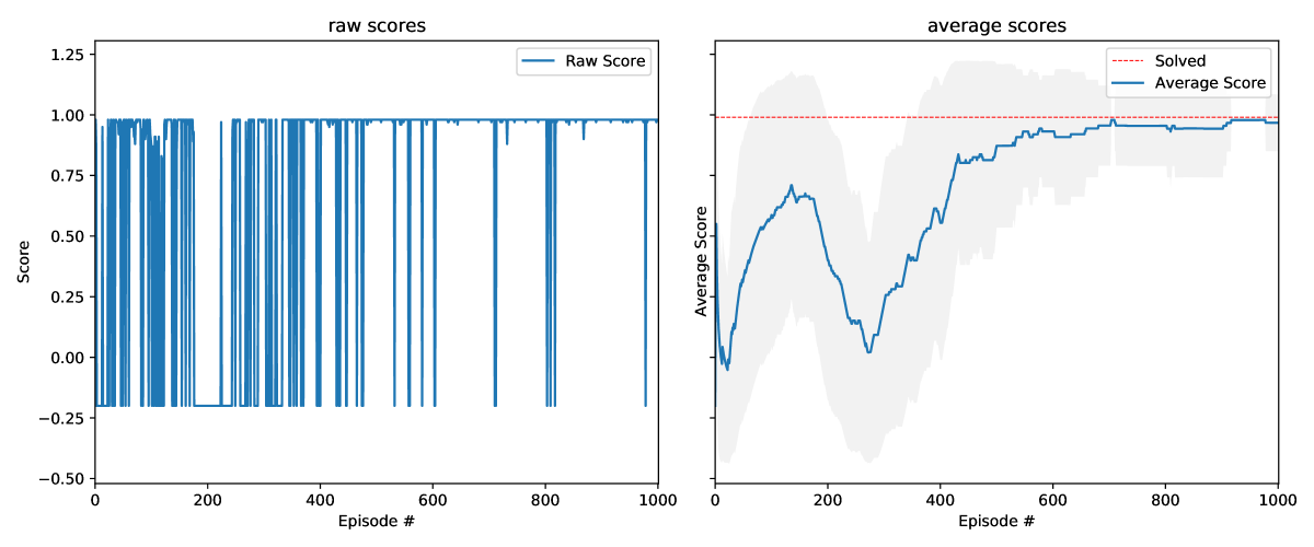
Figure 3: Environment-0 (Noise-Free) training-from-scratch simulation

To get the first policy for the PPR-algorithm such that its library would not be empty for the next task, we ran a simulation to solve for the Bell State circuit in a noise-free environment. This was done with just the DQN scheme as it is the first policy and there were no previous models to load into the library. From the results in Figure 3, we see that the DQN converges to the correct circuit solution around the $500^{th}$ episode when the score returned is close to $0.98$. The score is calculated according to Equation 3. This performance will serve as the benchmark (a control case of no noise) for comparisons to the more difficult environments, and the policy generated after the completion of the $1000^{th}$ episode will be added to the policy library to train the next policies.

VII.2 Environment 1: $0.01$ Noise on the $X$ Gate

Now that we have the policy from Environment-0 stored in our policy library, we can compare the two simulations involving Environment-1. The first is the training-from-scratch which shows how the agent performs under the environment with a regular DQN. Since the $X$-gate isn’t required in the circuit solution for the Bell State, it is not very surprising that the number of episodes to solve this noisy environment is around $400$ (which is less than the previous noise-free environment simply due to the stochastic nature of the agent). The note-worthy difference is between the training-from-scratch (Figure 4(a)) and the result using the PPR-algorithm (Figure 4(b)). We can see that the PPR-algorithm converges to the correct circuit solution considerably earlier (around $200$ episodes in) than in the training-from-scratch simulation.

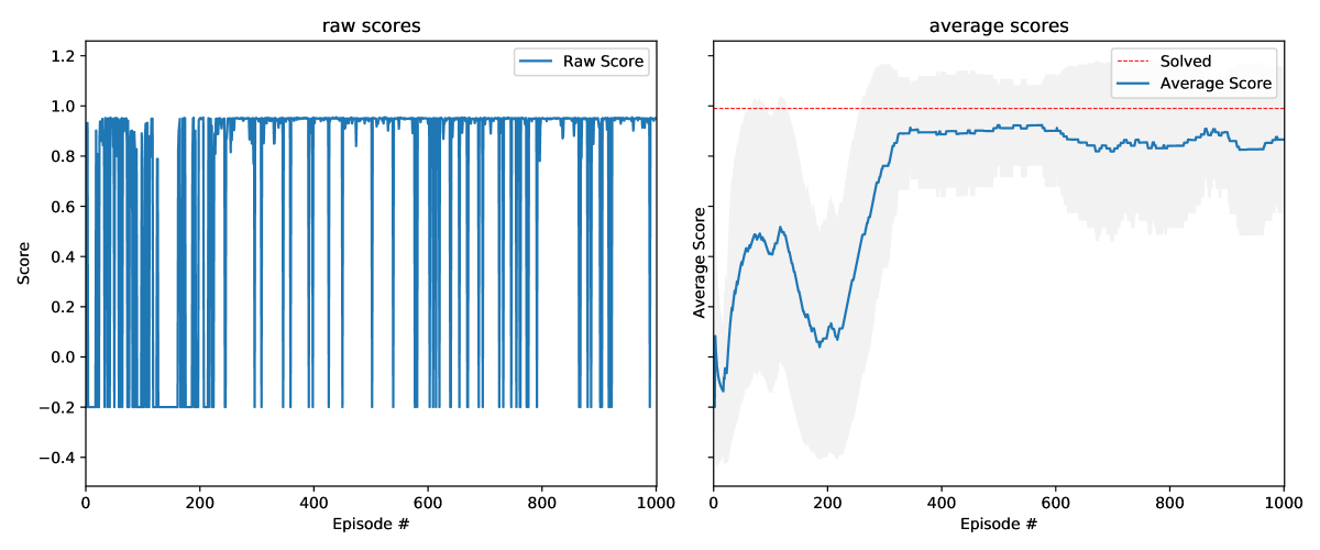
(a) Training-from-scratch simulation for Environment-1.

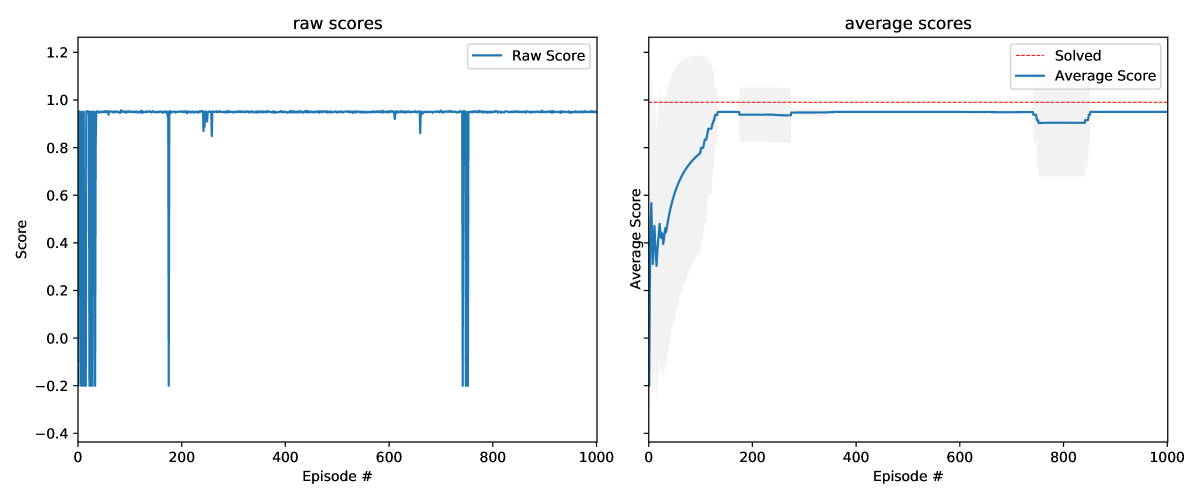
(b) Policy reuse simulation result for Environment-1.
Starting Policy Library: Simulation from Environment-0.

Figure 4: Training-from-scratch and policy reuse results for Environment-1: Noisy two-qubit system with single-qubit error rate $0.01$ on the $X$ gate and fidelity threshold $0.95$.

VII.3 Environment 2: $0.01$ Noise on the $X$ & $H$ Gates

Similarly for Environment-2, we see that the training-from-scratch (Figure 5(a)) had a more difficult time than in the previous two environments because there is now an added noise on one of the necessary components of the circuit solution. In the training-from-scratch, the agent converges to the correct solution around the $600^{th}$ episode while with the PPR-algorithm (Figure 5(b)) the agent reaches the right circuit in less than $200$ episodes. We can also see that even after reaching the final solution, the training-from-scratch (Figure 5(a)) is still fairly unstable whereas the policy reuse result (Figure 5(b)) converges and remains stable for the duration of the simulation. This makes the improvement with the PPR-algorithm even more apparent because it has taken a similar amount of time to solve what is a noticeably more challenging problem for the regular DQN learning scheme.

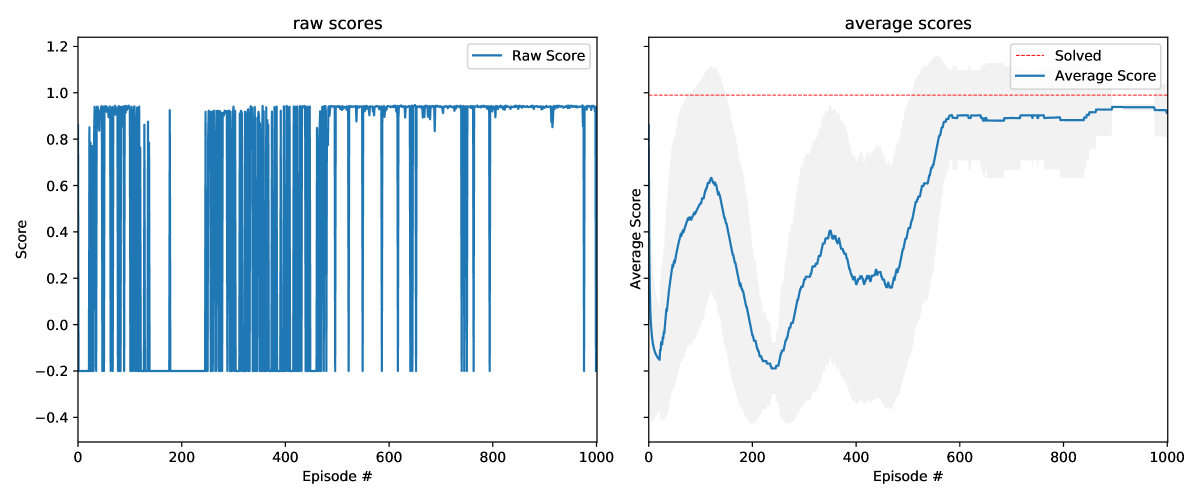
(a) Training-from-scratch simulation for Environment-2.

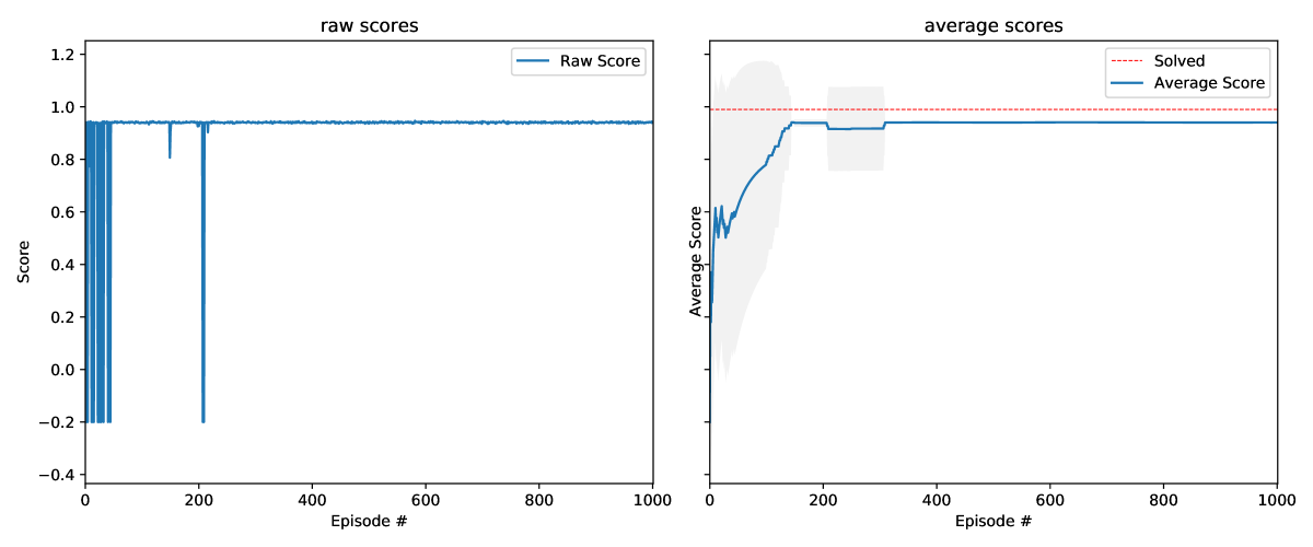
(b) Policy reuse simulation result for Environment-2.
Starting Policy Library: from Scratch - Environment-0, Policy Reuse - Environment-1.

Figure 5: Training-from-scratch and policy reuse results for Environment-2: Noisy two-qubit system with single-qubit error rate $0.01$ on the $X$ & $H$ gates and fidelity threshold $0.95$.

VII.4 Environment 3: $0.01$ Noise on the $X$ & $CNOT$ Gates

The next noise level involves the $CNOT$-gate, which affects both qubits and for that reason we expect it to be more challenging than the previous environments. We see that the training-from-scratch (Figure 6(a)) struggled to stabilize more with this added noise than in the previous environments, reaching the solution briefly around the $200^{th}$ episode but only stably getting the correct answer after episode $800$. Once again this highlights the performance of the PPR-algorithm (Figure 6(b)) since the agent again reaches the right circuit in less than $200$ episodes.

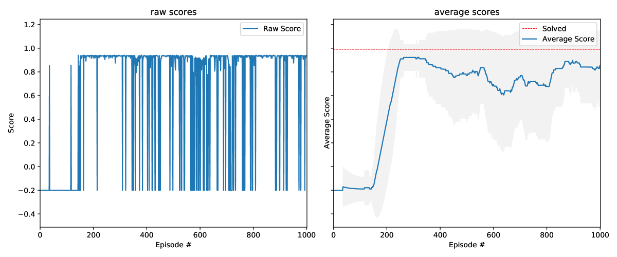
(a) Training-from-scratch simulation for Environment-3.

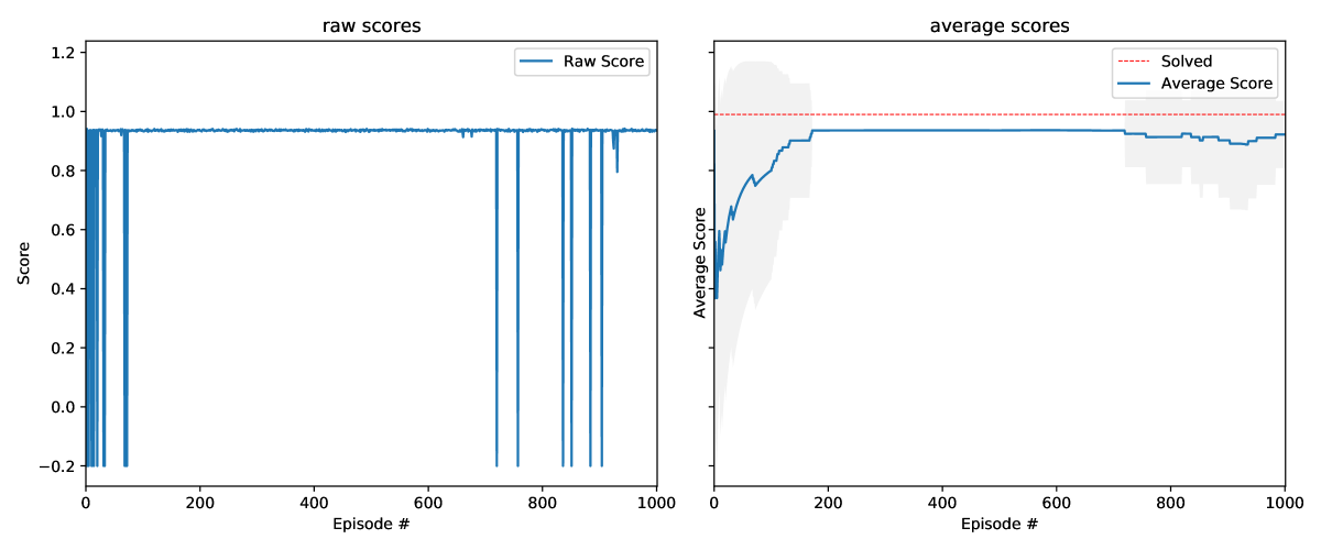
(b) Policy reuse simulation result for Environment-3.
Starting Policy Library: from Scratch - Environment-0, Policy Reuse - Environment-1, Policy Reuse - Environment-2.

Figure 6: Training-from-scratch and policy reuse results for Environment-3: Noisy two-qubit system with error rate $0.01$ on the $X$ & $CNOT$ gates and fidelity threshold $0.95$.

VII.5 Environment 4: $0.005$ Noise on the $X$, $H$, & $CNOT$ Gates

The noise level for this environment involves adding noise on three gates, which is more challenging than only two gates as we had in the previous environments. We see that the training-from-scratch (Figure 7(a)) again struggled to stabilize with this added noise but unlike the previous environment, the agent doesn’t appear to converge to the optimal solution within the 1000 episode time frame of the simulation. Conversely, we can see that the PPR-algorithm (Figure 7(b)) again reaches the right circuit in less than $200$ episodes and stabilizes very well.

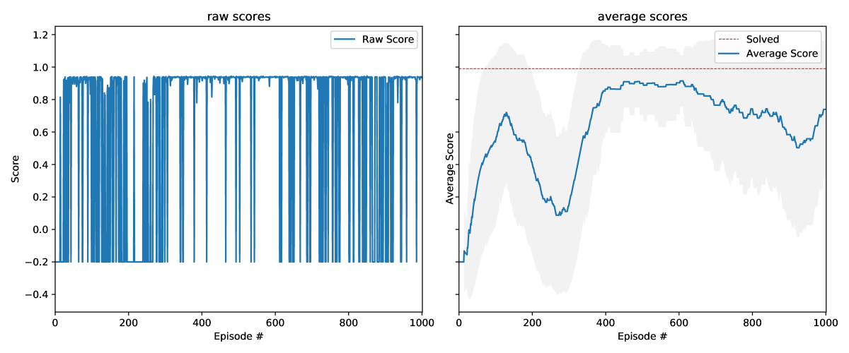
(a) Training-from-scratch simulation for Environment-4.

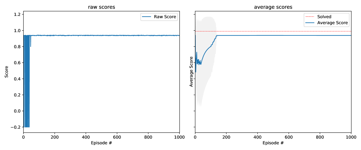
(b) Policy reuse simulation result for Environment-4.
Starting Policy Library: from Scratch - Environment-0, Policy Reuse - Environment-1, Policy Reuse - Environment-2, Policy Reuse - Environment-3.

Figure 7: Training-from-scratch and policy reuse results for Environment-4: Noisy two-qubit system with error rate $0.005$ on the $X$, $H$, & $CNOT$ gates and fidelity threshold $0.95$.

VII.6 Environment 5: $0.01$ Noise on the $X$ & $H$ Gates, $0.005$ on the $CNOT$ Gate

The noise level for this environment increases the amount of noise on two of the three gates, specifically the $X$ and $H$ gates, making it more difficult than Environment-4. We can see that the training-from-scratch (Figure 8(a)) is noticeably more unstable (dipping from $0.7$ to nearly $-0.2$ between episode $150$ to $300$). From the results of the PPR-algorithm (Figure 8(b)) we see that with the policy reuse, the agent performs much better and although there is some variation from the optimal solution, it is still a drastic improvement compared to the training-from-scratch (Figure 8(a)) and this deviation is understandable due to the difficulty of the noise in this environment.

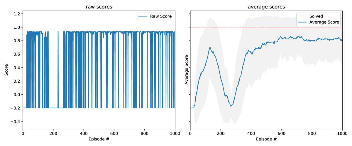
(a) Training-from-scratch simulation for Environment-5.

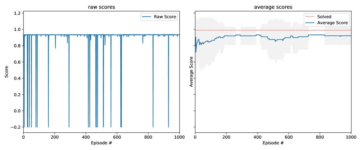
(b) Policy reuse simulation result for Environment-5.
Starting Policy Library: from Scratch - Environment-0, Policy Reuse - Environment-1, Policy Reuse - Environment-2, Policy Reuse - Environment-3, Policy Reuse - Environment-4.

Figure 8: Training-from-scratch and policy reuse results for Environment-5: Noisy two-qubit system with error rate $0.01$ on the $X$ & $H$ gates, error rate $0.005$ on the $CNOT$ gate, and fidelity threshold $0.95$.

VIII Discussion

VIII.1 Relevant Works

AI and ML techniques have been used to tackle certain challenges in quantum computing. Notable examples are quantum architecture search chen2021quantum , quantum error correction chen2019machine ; convy2021machine and quantum control zeng2020quantum . Among various ML techniques, RL is the one which draws a lot of attention since it is designed to solve complex sequential decision making problems and indeed, it has been applied in several recent works nautrup2019optimizing ; andreasson2019quantum ; colomer2020reinforcement ; sweke2020reinforcement . RL has been used to optimize existing quantum circuit architectures fosel2021quantum ; ostaszewski2021reinforcement . The idea is that there is a given ansatz of which the performance may not be optimal. The RL is used to modify the architecture by dropping some of the components or fine-tuning the circuit parameters fosel2021quantum ; ostaszewski2021reinforcement . The same logic is applied to optimizing existing quantum error correction codes nautrup2019optimizing ; andreasson2019quantum ; colomer2020reinforcement ; sweke2020reinforcement .

Our approach in this paper is different– we do not have an ansatz for the RL agent to optimize. On the contrary, the RL agent is trained to generate the quantum gate sequence from scratch, given only fidelity values and quantum measurement values. This task is expected to be harder than finding some potential modifications from existing non-optimal architectures. Indeed, the previous work kuo2021quantum considers this direction, providing a RL framework to find quantum architectures from scratch. However, for different tasks with various noise patterns, the RL agents need to be trained from scratch as well, making the workflow inefficient for constantly changing or drifting device noises and subsequently motivating our implementation of continual learning to address this problem.

VIII.2 Scalability

VIII.2.1 Policy Library

In this framework, the Policy Library grows with each run of the algorithm since each new task will be adding a new policy after completion. This becomes an issue, particularly for storage, as the number of tasks grows to be very large. With a large number of tasks, we would expect the Policy Library to contain a large number of policies and, in addition to storage, this effects the efficiency of the algorithm since it will need to sample from the large library set.

A possible solution to this is the use of eigenpolicies, which was proposed in the Fernandez paper fernandez2006probabilistic . Eigenpolicies operate on the principle that new policies which have a high similarity to a previous policy in the library will be absorbed by a principal eigenpolicy rather than occupy its own separate spot within the library.

In implementing the creation and maintaining of these eigenpolicies, the Policy Library can condense multiple policies by choosing whether it should store the newly generated policy as the start of a new eigenpolicy or absorb it into a previous entry.

Fascinatingly, this addition to the quantum circuit construction framework would allow for the existence of base circuit compositions. If we think of a classical computing analogy, the eigenpolicies would correspond to circuit blocks that can be readily reused to compose more complex, and larger-scale circuits. In other words, the eigenpolicies will correspond to a network of weights for a particular quantum state and if it is unique enough from other states, it will remain an eigenpolicy in the library and be used for problems that require it.

VIII.2.2 Action Space

In the framework detailed within this paper, the action space of the DQN (described in Equation 5) is coded such that each qubit has node for each gate in the set of given gates. This implies that as the number of qubits grows, the dimension of the action space grows non-linearly (due to the combinations of the $CNOT$ gates). For the general $n$-qubit case, there will be $5n+n(n-1)=\Omega(n^{2})$ actions. This makes scaling to a system with a large number of qubits fairly strenuous given that the action space is quadratic with respect to $n$. To counter this issue, a possible course of action is to have another level of network usage (one to generate the qubit index –which scales linearly– and the other to generate gates).

VIII.3 Training on a Real Quantum Computer

A necessary consideration for any research with simulated quantum computing is how well the work will translate to a real quantum computer. The current state of the quantum computers impose a realistic limitation on the number of gates that can be used on any given qubit due to the instability of the hardware and specifically, the severity of the error, which accumulates as more gates are added.

The work presented in this paper is designed to accommodate the IBM-Q interface and it would be trivial to apply the framework onto a real quantum computer. The more pressing concern with this decision lies in the state of the cloud-based facility. This includes the challenge of dealing with the unaltered device noise (as mentioned in Section VI.2) as well as the accessibility to the program while it is running. For RL in particular, many runs are required and these runs must be performed sequentially which can be challenging for a platform designed to be shared (in which jobs are queued). This, however, presents itself as more of a logistical or engineering problem and efforts are currently being made to develop tools which allow users more easily run experiments with many iterations on these cloud-based QC platforms (e.g. Qiskit Runtime).

VIII.4 Continual Learning with Policy Gradient Algorithms

A family of RL algorithms based on policy gradient methods are highly successful nowadays mnih2016asynchronous . Previously, it has been demonstrated that policy gradient algorithms can successfully implement the quantum architecture search objectives kuo2021quantum , quantum compiling herrera2021policy ; moro2021quantum and quantum control tasks baum2021experimental . One of the major challenges in training policy gradient RL agents is the sampling of a large amount of different paths (rollout), which requires significant computational resources. Therefore, there is a very strong motivation for continual learning to be implemented in those algorithms such that their usage can be optimized and further reduce the resource requirement of the problem. Continual RL in the context of policy gradients have been studied in works kim2021policy under standard RL tasks. It is interesting to study the potential of such algorithms in the challenging QAS tasks. We leave this for future investigation.

IX Conclusion

In this paper, we provide a framework to study how continual reinforcement learning can be applied to QAS problems. We showed numerically that the deep Q-learning with probabilistic policy reuse (PPR) lets the RL agent learn a good policy for the construction of a quantum gate sequence in various unseen environments. Furthermore, we demonstrate that the algorithm accomplishes this task within a significantly reduced number of training episodes through the leveraging of previously learned policies. The proposed framework is fairly general and can be applied to different types of quantum computing challenges. The result is especially useful when the underlying noise of the system is not well-understood. This in turn provides a promising implication to counter noise in quantum computers by enabling real-time autonomous corrections to the system in noisy environments in order to reach an arbitrary desired output state.

Appendix A Appendixes

Define the transition pair to be in the form $(s_{t},a_{t},r_{t},s_{t+1})$

Given an environment, $\mathcal{E}$

Given the replay memory, $\mathcal{D}$

Given a new policy, $L_{0}$

Given the maximum number of episodes to execute, $K$

Given the maximum number of steps per episode, $H$

Initialize the rewards list $W$

for episode $=1,2,\ldots,K$ do

     Reset the environment $\mathcal{E}$

     for $t=1,2,\ldots,H$ do

         Select action $a_{t}$ from $L_{0}$ using greedy policy selection

         Perform the action $a_{t}$

         Observe the new state $s_{t+1}$

         if not done:

          Assign the next state in the transition pair to be the new state $s_{t+1}$

         else:

          Assign the next state in the transition pair to be none

         Store the transition pair to $\mathcal{D}$ and assign current state $s$ to be next state $s_{t+1}$

         Optimize $L_{0}$

         if done:

          Update $W$

          break

     end for

end for

Return mean($W$), new policy $L_{0}$

Algorithm 1 q-learning algorithm

Define the transition pair to be in the form $(s_{t},a_{t},r_{t},s_{t+1})$

Given an environment, $\mathcal{E}$

Given the replay memory, $\mathcal{D}$

Given a past policy to try $L_{i}$ and the new policy $L_{0}$

Given the maximum number of episodes to execute, $K$

Given the maximum number of steps per episode, $H$

Given the parameters $\psi$ and $\nu$

Initialize the rewards list $W$

for episode $=1,2,\ldots,K$ do

     Reset the environment $\mathcal{E}$

     for $t$ $=1,2,\ldots,H$ do

         Sample a random probability $p$

         if $p<=\psi$

          Select action $a_{t}$ from $L_{i}$ using greedy policy selection

         else:

          Select action $a_{t}$ from $L_{0}$ using greedy policy selection

         Perform the action $a_{t}$

         Observe the new state $s_{t+1}$

         Update $\psi$ to be $\psi\cdot\nu$

         if not done:

          Assign the next state in the transition pair to be the new state $s_{t+1}$

         else:

          Assign the next state in the transition pair to be none

         Store the transition pair to $\mathcal{D}$ and assign current state to be next state

         Optimize $L_{0}$

         if done:

          Update $W$

          break

     end for

end for

Return mean($W$), new policy $L_{0}$

Algorithm 2 $\pi$-exploration algorithm

Given a new task $\Omega$ we want to solve

Given a policy library $L=\{\Pi_{1},\cdots,\Pi_{n}\}$

Given an initial temperature parameter $\tau$ and the incremental size $\delta\tau$ for the Boltzmann policy selection strategy

Given the maximum number of episodes to execute, $K$

Given the maximum number of steps per episode, $H$

Given the parameters $\psi$ and $\nu$ for the $\pi$-exploration strategy

Initialize replay memory $\mathcal{D}$ to capacity $N$

Initialize a new policy $L_{0}$

Initialize a target policy $\hat{L}_{0}=L_{0}$

Initialize target network update rate, $T$

Initialize the rewards $W_{i}$ to $0$

Initialize the number of episodes where policy $\Pi_{i}$ has been chosen, $U_{i}=0,\forall i=1,\cdots,n$

for episode $=1,2,\ldots,K$ do

     Get probability vector $p$ from softmax function inputting $W$ and $\tau$

     Sample from $p$ to get an index for the action policy $k$

     if $k==0$:

      Use the q-learning algorithm to get rewards $R$ and $L_{0}$

     else:

      Use the $\pi$-exploration algorithm to get $R,\ L_{0}$

     Update $W_{k}\leftarrow\frac{W_{k}\cdot U_{k}+R}{U_{k}+1}$

     Update $U_{k}\leftarrow U_{k}+1$

     Update $\tau\leftarrow\tau+\delta\tau$

     if episode is divisible by $T$:

      Update $\hat{L}_{0}$ with $L_{0}$

end for

Algorithm 3 Probabilistic Policy Reuse with deep Q learning

References

- (1) R. P. Feynman, “Quantum mechanical computers,” Optics news, vol. 11, no. 2, pp. 11–20, 1985.
- (2) A. W. Harrow and A. Montanaro, “Quantum computational supremacy,” Nature, vol. 549, no. 7671, pp. 203–209, 2017.
- (3) F. Arute, K. Arya, R. Babbush, D. Bacon, J. C. Bardin, R. Barends, R. Biswas, S. Boixo, F. G. Brandao, D. A. Buell, et al., “Quantum supremacy using a programmable superconducting processor,” Nature, vol. 574, no. 7779, pp. 505–510, 2019.
- (4) M. A. Nielsen and I. Chuang, “Quantum computation and quantum information,” 2002.
- (5) P. W. Shor, “Polynomial-time algorithms for prime factorization and discrete logarithms on a quantum computer,” SIAM review, vol. 41, no. 2, pp. 303–332, 1999.
- (6) L. K. Grover, “Quantum mechanics helps in searching for a needle in a haystack,” Physical review letters, vol. 79, no. 2, p. 325, 1997.
- (7) J. Preskill, “Quantum computing in the nisq era and beyond,” Quantum, vol. 2, p. 79, 2018.
- (8) D. Gottesman, “Stabilizer codes and quantum error correction,” arXiv preprint quant-ph/9705052, 1997.
- (9) D. Gottesman, “Theory of fault-tolerant quantum computation,” Physical Review A, vol. 57, no. 1, p. 127, 1998.
- (10) M. Cerezo, A. Arrasmith, R. Babbush, S. C. Benjamin, S. Endo, K. Fujii, J. R. McClean, K. Mitarai, X. Yuan, L. Cincio, et al., “Variational quantum algorithms,” arXiv preprint arXiv:2012.09265, 2020.
- (11) K. Bharti, A. Cervera-Lierta, T. H. Kyaw, T. Haug, S. Alperin-Lea, A. Anand, M. Degroote, H. Heimonen, J. S. Kottmann, T. Menke, et al., “Noisy intermediate-scale quantum (nisq) algorithms,” arXiv preprint arXiv:2101.08448, 2021.
- (12) A. Peruzzo, J. McClean, P. Shadbolt, M.-H. Yung, X.-Q. Zhou, P. J. Love, A. Aspuru-Guzik, and J. L. O’brien, “A variational eigenvalue solver on a photonic quantum processor,” Nature communications, vol. 5, p. 4213, 2014.
- (13) S. Y.-C. Chen, S. Yoo, and Y.-L. L. Fang, “Quantum long short-term memory,” arXiv preprint arXiv:2009.01783, 2020.
- (14) K. Mitarai, M. Negoro, M. Kitagawa, and K. Fujii, “Quantum circuit learning,” Physical Review A, vol. 98, no. 3, p. 032309, 2018.
- (15) A. E. Paine, V. E. Elfving, and O. Kyriienko, “Quantum quantile mechanics: Solving stochastic differential equations for generating time-series,” 2021.
- (16) O. Kyriienko, A. E. Paine, and V. E. Elfving, “Solving nonlinear differential equations with differentiable quantum circuits,” Physical Review A, vol. 103, no. 5, p. 052416, 2021.
- (17) M. Schuld, A. Bocharov, K. Svore, and N. Wiebe, “Circuit-centric quantum classifiers,” arXiv preprint arXiv:1804.00633, 2018.
- (18) V. Havlíček, A. D. Córcoles, K. Temme, A. W. Harrow, A. Kandala, J. M. Chow, and J. M. Gambetta, “Supervised learning with quantum-enhanced feature spaces,” Nature, vol. 567, no. 7747, pp. 209–212, 2019.
- (19) E. Farhi and H. Neven, “Classification with quantum neural networks on near term processors,” arXiv preprint arXiv:1802.06002, 2018.
- (20) M. Benedetti, E. Lloyd, S. Sack, and M. Fiorentini, “Parameterized quantum circuits as machine learning models,” Quantum Science and Technology, vol. 4, no. 4, p. 043001, 2019.
- (21) A. Mari, T. R. Bromley, J. Izaac, M. Schuld, and N. Killoran, “Transfer learning in hybrid classical-quantum neural networks,” arXiv preprint arXiv:1912.08278, 2019.
- (22) Z. Abohashima, M. Elhosen, E. H. Houssein, and W. M. Mohamed, “Classification with quantum machine learning: A survey,” arXiv preprint arXiv:2006.12270, 2020.
- (23) P. Easom-McCaldin, A. Bouridane, A. Belatreche, and R. Jiang, “Towards building a facial identification system using quantum machine learning techniques,” arXiv preprint arXiv:2008.12616, 2020.
- (24) A. Sarma, R. Chatterjee, K. Gili, and T. Yu, “Quantum unsupervised and supervised learning on superconducting processors,” arXiv preprint arXiv:1909.04226, 2019.
- (25) S. A. Stein, B. Baheri, R. M. Tischio, Y. Chen, Y. Mao, Q. Guan, A. Li, and B. Fang, “A hybrid system for learning classical data in quantum states,” arXiv preprint arXiv:2012.00256, 2020.
- (26) S. Y.-C. Chen, C.-M. Huang, C.-W. Hsing, and Y.-J. Kao, “An end-to-end trainable hybrid classical-quantum classifier,” Machine Learning: Science and Technology, 2021.
- (27) S. Y.-C. Chen, T.-C. Wei, C. Zhang, H. Yu, and S. Yoo, “Quantum convolutional neural networks for high energy physics data analysis,” arXiv preprint arXiv:2012.12177, 2020.
- (28) S. L. Wu, J. Chan, W. Guan, S. Sun, A. Wang, C. Zhou, M. Livny, F. Carminati, A. Di Meglio, A. C. Li, et al., “Application of quantum machine learning using the quantum variational classifier method to high energy physics analysis at the lhc on ibm quantum computer simulator and hardware with 10 qubits,” Journal of Physics G: Nuclear and Particle Physics, 2021.
- (29) S. A. Stein, Y. Mao, B. Baheri, Q. Guan, A. Li, D. Chen, S. Xu, and C. Ding, “Quclassi: A hybrid deep neural network architecture based on quantum state fidelity,” arXiv preprint arXiv:2103.11307, 2021.
- (30) S. Y.-C. Chen, T.-C. Wei, C. Zhang, H. Yu, and S. Yoo, “Hybrid quantum-classical graph convolutional network,” arXiv preprint arXiv:2101.06189, 2021.
- (31) B. Jaderberg, L. W. Anderson, W. Xie, S. Albanie, M. Kiffner, and D. Jaksch, “Quantum self-supervised learning,” arXiv preprint arXiv:2103.14653, 2021.
- (32) D. Mattern, D. Martyniuk, H. Willems, F. Bergmann, and A. Paschke, “Variational quanvolutional neural networks with enhanced image encoding,” arXiv preprint arXiv:2106.07327, 2021.
- (33) T. Hur, L. Kim, and D. K. Park, “Quantum convolutional neural network for classical data classification,” arXiv preprint arXiv:2108.00661, 2021.
- (34) W. Li and D.-L. Deng, “Recent advances for quantum classifiers,” arXiv preprint arXiv:2108.13421, 2021.
- (35) P.-L. Dallaire-Demers and N. Killoran, “Quantum generative adversarial networks,” Physical Review A, vol. 98, no. 1, p. 012324, 2018.
- (36) S. A. Stein, B. Baheri, R. M. Tischio, Y. Mao, Q. Guan, A. Li, B. Fang, and S. Xu, “Qugan: A generative adversarial network through quantum states,” arXiv preprint arXiv:2010.09036, 2020.
- (37) C. Zoufal, A. Lucchi, and S. Woerner, “Quantum generative adversarial networks for learning and loading random distributions,” npj Quantum Information, vol. 5, no. 1, pp. 1–9, 2019.
- (38) H. Situ, Z. He, L. Li, and S. Zheng, “Quantum generative adversarial network for generating discrete data,” arXiv preprint arXiv:1807.01235, 2018.
- (39) K. Nakaji and N. Yamamoto, “Quantum semi-supervised generative adversarial network for enhanced data classification,” arXiv preprint arXiv:2010.13727, 2020.
- (40) S. Y.-C. Chen, C.-H. H. Yang, J. Qi, P.-Y. Chen, X. Ma, and H.-S. Goan, “Variational quantum circuits for deep reinforcement learning,” IEEE Access, vol. 8, pp. 141007–141024, 2020.
- (41) O. Lockwood and M. Si, “Reinforcement learning with quantum variational circuit,” in Proceedings of the AAAI Conference on Artificial Intelligence and Interactive Digital Entertainment, vol. 16, pp. 245–251, 2020.
- (42) S. Jerbi, L. M. Trenkwalder, H. P. Nautrup, H. J. Briegel, and V. Dunjko, “Quantum enhancements for deep reinforcement learning in large spaces,” PRX Quantum, vol. 2, no. 1, p. 010328, 2021.
- (43) C.-C. CHEN, K. SHIBA, M. SOGABE, K. SAKAMOTO, and T. SOGABE, “Hybrid quantum-classical ulam-von neumann linear solver-based quantum dynamic programing algorithm,” Proceedings of the Annual Conference of JSAI, vol. JSAI2020, pp. 2K6ES203–2K6ES203, 2020.
- (44) S. Wu, S. Jin, D. Wen, and X. Wang, “Quantum reinforcement learning in continuous action space,” arXiv preprint arXiv:2012.10711, 2020.
- (45) A. Skolik, S. Jerbi, and V. Dunjko, “Quantum agents in the gym: a variational quantum algorithm for deep q-learning,” arXiv preprint arXiv:2103.15084, 2021.
- (46) S. Jerbi, C. Gyurik, S. Marshall, H. J. Briegel, and V. Dunjko, “Variational quantum policies for reinforcement learning,” arXiv preprint arXiv:2103.05577, 2021.
- (47) Y. Kwak, W. J. Yun, S. Jung, J.-K. Kim, and J. Kim, “Introduction to quantum reinforcement learning: Theory and pennylane-based implementation,” arXiv preprint arXiv:2108.06849, 2021.
- (48) D. Nagy, Z. Tabi, P. Hága, Z. Kallus, and Z. Zimborás, “Photonic quantum policy learning in openai gym,” arXiv preprint arXiv:2108.12926, 2021.
- (49) S. Y.-C. Chen, C.-M. Huang, C.-W. Hsing, H.-S. Goan, and Y.-J. Kao, “Variational quantum reinforcement learning via evolutionary optimization,” arXiv preprint arXiv:2109.00540, 2021.
- (50) J. Bausch, “Recurrent quantum neural networks,” arXiv preprint arXiv:2006.14619, 2020.
- (51) Y. Takaki, K. Mitarai, M. Negoro, K. Fujii, and M. Kitagawa, “Learning temporal data with variational quantum recurrent neural network,” arXiv preprint arXiv:2012.11242, 2020.
- (52) M. Abbaszade, V. Salari, S. S. Mousavi, M. Zomorodi, and X. Zhou, “Application of quantum natural language processing for language translation,” IEEE Access, 2021.
- (53) C.-H. H. Yang, J. Qi, S. Y.-C. Chen, P.-Y. Chen, S. M. Siniscalchi, X. Ma, and C.-H. Lee, “Decentralizing feature extraction with quantum convolutional neural network for automatic speech recognition,” in ICASSP 2021-2021 IEEE International Conference on Acoustics, Speech and Signal Processing (ICASSP), pp. 6523–6527, IEEE, 2021.
- (54) S. Lloyd, M. Schuld, A. Ijaz, J. Izaac, and N. Killoran, “Quantum embeddings for machine learning,” arXiv preprint arXiv:2001.03622, 2020.
- (55) N. A. Nghiem, S. Y.-C. Chen, and T.-C. Wei, “Unified framework for quantum classification,” Physical Review Research, vol. 3, no. 3, p. 033056, 2021.
- (56) S. Y.-C. Chen and S. Yoo, “Federated quantum machine learning,” Entropy, vol. 23, no. 4, p. 460, 2021.
- (57) M. Chehimi and W. Saad, “Quantum federated learning with quantum data,” arXiv preprint arXiv:2106.00005, 2021.
- (58) Y. LeCun, Y. Bengio, and G. Hinton, “Deep learning,” nature, vol. 521, no. 7553, pp. 436–444, 2015.
- (59) I. Goodfellow, Y. Bengio, and A. Courville, Deep learning. MIT press, 2016.
- (60) A. Voulodimos, N. Doulamis, A. Doulamis, and E. Protopapadakis, “Deep learning for computer vision: A brief review,” Computational intelligence and neuroscience, vol. 2018, 2018.
- (61) K. Simonyan and A. Zisserman, “Very deep convolutional networks for large-scale image recognition,” arXiv preprint arXiv:1409.1556, 2014.
- (62) Y. LeCun, L. Bottou, Y. Bengio, and P. Haffner, “Gradient-based learning applied to document recognition,” Proceedings of the IEEE, vol. 86, no. 11, pp. 2278–2324, 1998.
- (63) D. Bahdanau, K. Cho, and Y. Bengio, “Neural machine translation by jointly learning to align and translate,” arXiv preprint arXiv:1409.0473, 2014.
- (64) A. Vaswani, N. Shazeer, N. Parmar, J. Uszkoreit, L. Jones, A. N. Gomez, Ł. Kaiser, and I. Polosukhin, “Attention is all you need,” in Advances in neural information processing systems, pp. 5998–6008, 2017.
- (65) T. Young, D. Hazarika, S. Poria, and E. Cambria, “Recent trends in deep learning based natural language processing,” ieee Computational intelligenCe magazine, vol. 13, no. 3, pp. 55–75, 2018.
- (66) D. W. Otter, J. R. Medina, and J. K. Kalita, “A survey of the usages of deep learning for natural language processing,” IEEE Transactions on Neural Networks and Learning Systems, vol. 32, no. 2, pp. 604–624, 2020.
- (67) V. Mnih, K. Kavukcuoglu, D. Silver, A. A. Rusu, J. Veness, M. G. Bellemare, A. Graves, M. Riedmiller, A. K. Fidjeland, G. Ostrovski, et al., “Human-level control through deep reinforcement learning,” nature, vol. 518, no. 7540, pp. 529–533, 2015.
- (68) D. Silver, J. Schrittwieser, K. Simonyan, I. Antonoglou, A. Huang, A. Guez, T. Hubert, L. Baker, M. Lai, A. Bolton, et al., “Mastering the game of go without human knowledge,” nature, vol. 550, no. 7676, pp. 354–359, 2017.
- (69) D. Silver, A. Huang, C. J. Maddison, A. Guez, L. Sifre, G. Van Den Driessche, J. Schrittwieser, I. Antonoglou, V. Panneershelvam, M. Lanctot, et al., “Mastering the game of go with deep neural networks and tree search,” nature, vol. 529, no. 7587, pp. 484–489, 2016.
- (70) J. Schrittwieser, I. Antonoglou, T. Hubert, K. Simonyan, L. Sifre, S. Schmitt, A. Guez, E. Lockhart, D. Hassabis, T. Graepel, et al., “Mastering atari, go, chess and shogi by planning with a learned model,” arXiv preprint arXiv:1911.08265, 2019.
- (71) A. P. Badia, B. Piot, S. Kapturowski, P. Sprechmann, A. Vitvitskyi, D. Guo, and C. Blundell, “Agent57: Outperforming the atari human benchmark,” arXiv preprint arXiv:2003.13350, 2020.
- (72) R. S. Sutton and A. G. Barto, Reinforcement learning: An introduction. MIT press, 2018.
- (73) D. Bertsekas, Rollout, policy iteration, and distributed reinforcement learning. Athena Scientific, 2021.
- (74) H. P. Nautrup, N. Delfosse, V. Dunjko, H. J. Briegel, and N. Friis, “Optimizing quantum error correction codes with reinforcement learning,” Quantum, vol. 3, p. 215, 2019.
- (75) P. Andreasson, J. Johansson, S. Liljestrand, and M. Granath, “Quantum error correction for the toric code using deep reinforcement learning,” Quantum, vol. 3, p. 183, 2019.
- (76) L. D. Colomer, M. Skotiniotis, and R. Muñoz-Tapia, “Reinforcement learning for optimal error correction of toric codes,” Physics Letters A, vol. 384, no. 17, p. 126353, 2020.
- (77) R. Sweke, M. S. Kesselring, E. P. van Nieuwenburg, and J. Eisert, “Reinforcement learning decoders for fault-tolerant quantum computation,” Machine Learning: Science and Technology, vol. 2, no. 2, p. 025005, 2020.
- (78) M. Y. Niu, S. Boixo, V. N. Smelyanskiy, and H. Neven, “Universal quantum control through deep reinforcement learning,” npj Quantum Information, vol. 5, no. 1, pp. 1–8, 2019.
- (79) Z. An and D. Zhou, “Deep reinforcement learning for quantum gate control,” EPL (Europhysics Letters), vol. 126, no. 6, p. 60002, 2019.
- (80) M. Bukov, A. G. Day, D. Sels, P. Weinberg, A. Polkovnikov, and P. Mehta, “Reinforcement learning in different phases of quantum control,” Physical Review X, vol. 8, no. 3, p. 031086, 2018.
- (81) T. Fösel, P. Tighineanu, T. Weiss, and F. Marquardt, “Reinforcement learning with neural networks for quantum feedback,” Physical Review X, vol. 8, no. 3, p. 031084, 2018.
- (82) X.-M. Zhang, Z. Wei, R. Asad, X.-C. Yang, and X. Wang, “When does reinforcement learning stand out in quantum control? a comparative study on state preparation,” npj Quantum Information, vol. 5, no. 1, pp. 1–7, 2019.
- (83) P. Palittapongarnpim, P. Wittek, E. Zahedinejad, S. Vedaie, and B. C. Sanders, “Learning in quantum control: High-dimensional global optimization for noisy quantum dynamics,” Neurocomputing, vol. 268, pp. 116–126, 2017.
- (84) H. Xu, J. Li, L. Liu, Y. Wang, H. Yuan, and X. Wang, “Generalizable control for quantum parameter estimation through reinforcement learning,” npj Quantum Information, vol. 5, no. 1, pp. 1–8, 2019.
- (85) J. Brown, P. Sgroi, L. Giannelli, G. S. Paraoanu, E. Paladino, G. Falci, M. Paternostro, and A. Ferraro, “Reinforcement learning-enhanced protocols for coherent population-transfer in three-level quantum systems,” New Journal of Physics, 2021.
- (86) Y. Baum, M. Amico, S. Howell, M. Hush, M. Liuzzi, P. Mundada, T. Merkh, A. R. Carvalho, and M. J. Biercuk, “Experimental deep reinforcement learning for error-robust gateset design on a superconducting quantum computer,” arXiv preprint arXiv:2105.01079, 2021.
- (87) K. He, X. Zhang, S. Ren, and J. Sun, “Deep residual learning for image recognition,” in Proceedings of the IEEE conference on computer vision and pattern recognition, pp. 770–778, 2016.
- (88) B. Zoph and Q. V. Le, “Neural architecture search with reinforcement learning,” arXiv preprint arXiv:1611.01578, 2016.
- (89) B. Baker, O. Gupta, N. Naik, and R. Raskar, “Designing neural network architectures using reinforcement learning,” arXiv preprint arXiv:1611.02167, 2016.
- (90) H. Cai, T. Chen, W. Zhang, Y. Yu, and J. Wang, “Efficient architecture search by network transformation,” arXiv preprint arXiv:1707.04873, 2017.
- (91) B. Zoph, V. Vasudevan, J. Shlens, and Q. V. Le, “Learning transferable architectures for scalable image recognition,” in Proceedings of the IEEE conference on computer vision and pattern recognition, pp. 8697–8710, 2018.
- (92) Z. Zhong, J. Yan, W. Wu, J. Shao, and C.-L. Liu, “Practical block-wise neural network architecture generation,” in Proceedings of the IEEE conference on computer vision and pattern recognition, pp. 2423–2432, 2018.
- (93) M. Schrimpf, S. Merity, J. Bradbury, and R. Socher, “A flexible approach to automated rnn architecture generation,” arXiv preprint arXiv:1712.07316, 2017.
- (94) H. Pham, M. Y. Guan, B. Zoph, Q. V. Le, and J. Dean, “Efficient neural architecture search via parameter sharing,” arXiv preprint arXiv:1802.03268, 2018.
- (95) H. Cai, J. Yang, W. Zhang, S. Han, and Y. Yu, “Path-level network transformation for efficient architecture search,” arXiv preprint arXiv:1806.02639, 2018.
- (96) T. Elsken, J. H. Metzen, F. Hutter, et al., “Neural architecture search: A survey.,” J. Mach. Learn. Res., vol. 20, no. 55, pp. 1–21, 2019.
- (97) M. Ostaszewski, L. M. Trenkwalder, W. Masarczyk, E. Scerri, and V. Dunjko, “Reinforcement learning for optimization of variational quantum circuit architectures,” arXiv preprint arXiv:2103.16089, 2021.
- (98) T. Fösel, M. Y. Niu, F. Marquardt, and L. Li, “Quantum circuit optimization with deep reinforcement learning,” arXiv preprint arXiv:2103.07585, 2021.
- (99) M. Pirhooshyaran and T. Terlaky, “Quantum circuit design search,” arXiv preprint arXiv:2012.04046, 2020.
- (100) A. Bolens and M. Heyl, “Reinforcement learning for digital quantum simulation,” Physical Review Letters, vol. 127, no. 11, p. 110502, 2021.
- (101) E.-J. Kuo, Y.-L. L. Fang, and S. Y.-C. Chen, “Quantum architecture search via deep reinforcement learning,” arXiv preprint arXiv:2104.07715, 2021.
- (102) V. Mnih, A. P. Badia, M. Mirza, A. Graves, T. Lillicrap, T. Harley, D. Silver, and K. Kavukcuoglu, “Asynchronous methods for deep reinforcement learning,” in International conference on machine learning, pp. 1928–1937, PMLR, 2016.
- (103) E. Bengio, J. Pineau, and D. Precup, “Interference and generalization in temporal difference learning,” in International Conference on Machine Learning, pp. 767–777, PMLR, 2020.
- (104) M. B. Ring, “Child: A first step towards continual learning,” in Learning to learn, pp. 261–292, Springer, 1998.
- (105) F. Fernández and M. Veloso, “Probabilistic policy reuse in a reinforcement learning agent,” in Proceedings of the fifth international joint conference on Autonomous agents and multiagent systems, pp. 720–727, 2006.
- (106) D. P. Kingma and J. Ba, “Adam: A method for stochastic optimization,” arXiv preprint arXiv:1412.6980, 2014.
- (107) A. Paszke, “Reinforcement learning (dqn) tutorial.” https://pytorch.org/tutorials/intermediate/reinforcement_q_learning.html.
- (108) C. Chen, Z. He, L. Li, S. Zheng, and H. Situ, “Quantum architecture search with meta-learning,” arXiv preprint arXiv:2106.06248, 2021.
- (109) H. Chen, M. Vasmer, N. P. Breuckmann, and E. Grant, “Machine learning logical gates for quantum error correction,” arXiv preprint arXiv:1912.10063, 2019.
- (110) I. Convy, H. Liao, S. Zhang, S. Patel, W. P. Livingston, H. N. Nguyen, I. Siddiqi, and K. B. Whaley, “Machine learning for continuous quantum error correction on superconducting qubits,” arXiv preprint arXiv:2110.10378, 2021.
- (111) Y. Zeng, J. Shen, S. Hou, T. Gebremariam, and C. Li, “Quantum control based on machine learning in an open quantum system,” Physics Letters A, vol. 384, no. 35, p. 126886, 2020.
- (112) D. A. Herrera-Martí, “Policy gradient approach to compilation of variational quantum circuits,” arXiv preprint arXiv:2111.10227, 2021.
- (113) L. Moro, M. G. Paris, M. Restelli, and E. Prati, “Quantum compiling by deep reinforcement learning,” arXiv preprint arXiv:2105.15048, 2021.
- (114) D. K. Kim, M. Liu, M. D. Riemer, C. Sun, M. Abdulhai, G. Habibi, S. Lopez-Cot, G. Tesauro, and J. How, “A policy gradient algorithm for learning to learn in multiagent reinforcement learning,” in International Conference on Machine Learning, pp. 5541–5550, PMLR, 2021.