Spinning cylinders in general relativity: a canonical form for the Lewis metrics of the Weyl class

Abstract

In the main article [CQG 38 (2021) 055003], a new “canonical” form for the Lewis metrics of the Weyl class has been obtained, depending only on three parameters — Komar mass and angular momentum per unit length, plus the angle deficit — corresponding to a coordinate system fixed to the “distant stars” and an everywhere timelike Killing vector field. Such form evinces the local but non-global static character of the spacetime, and striking parallelisms with the electromagnetic analogue. We discuss here its generality, main physical features and important limits (the Levi-Civita static cylinder, and spinning cosmic strings). We contrast it on geometric and physical grounds with the Kerr spacetime — as an example of a metric which is locally non-static.

Keywords: gravitomagnetism; 1+3 quasi-Maxwell formalism; Sagnac effect; gravitomagnetic clock effect; synchronization gap; local and global staticity; Levi-Civita solution; cosmic strings

1 Introduction

The general stationary solution of the vacuum Einstein field equations with cylindrical symmetry are the Lewis metrics [1, 2, 3, 4]

$$ds^{2}=-f(dt^{2}+Cd\varphi)^{2}+r^{(n^{2}-1)/2}(dr^{2}+dz^{2})+\frac{r^{2}}{f}d\varphi^{2}\ ;$$ (1)

$$f=ar^{1-n}-\frac{c^{2}r^{n+1}}{n^{2}a}\ ;\qquad C=\frac{cr^{n+1}}{naf}+b\ ,$$ (2)

usually interpreted as describing the exterior gravitational field produced by infinitely long rotating cylinders. They divide into two classes: (i) the Weyl class, when all the constants $n$, $a$, $b$, and $c$ are real; (ii) the Lewis class, for $n$ imaginary [implying in turn $c$ real and $a$ and $b$ complex, in order for the line element (1) to be real[4, 3]].

In the main article, Ref. [5], we have shown that the Weyl class metrics can be written in the “canonical” form

$$ds^{2}=-\frac{r^{4\lambda_{{\rm m}}}}{\alpha}\left(dt-\frac{j}{\lambda_{{\rm m}}-1/4}d\phi\right)^{2}+r^{4\lambda_{{\rm m}}(2\lambda_{{\rm m}}-1)}(dr^{2}+dz^{2})+\alpha r^{2(1-2\lambda_{{\rm m}})}d\phi^{2}\ ,$$

depending only on three parameters with a clear physical significance: the Komar mass ($\lambda_{{\rm m}}$) and angular momentum ($j$) per unit $z$-length, plus the parameter $\alpha$ governing the angle deficit. This form allows for a transparent comparison with the Levi-Civita non-rotating cylinder — archetype of the contrast between local and global staticity — which Ref. [5] discusses in detail both on physical and geometrical grounds. Therein its matching to the van Stockum [6] cylinder in star fixed coordinates is also shown. Here we revise some main features of the solution, focusing on its generality [and redundancies of the more usual form (1)-(2)], notable limits, and physical properties, with special attention to those less developed in Ref. [5]. Addressing the question posed to us in the discussion following the presentation of this work at MG16[7], we focus here on its comparison with a non-static (globally and locally) stationary solution, exemplified by the Kerr spacetime.

2 Stationary spacetimes and levels of gravitomagnetism

The line element $ds^{2}=g_{\alpha\beta}dx^{\alpha}dx^{\beta}$ of a stationary spacetime can generically be written as

$$ds^{2}=-e^{2\Phi}(dt-\mathcal{A}_{i}dx^{i})^{2}+h_{ij}dx^{i}dx^{j}\ ,$$ (3)

where $e^{2\Phi}=-g_{00}$, $\Phi\equiv\Phi(x^{j})$, $\mathcal{A}_{i}\equiv\mathcal{A}_{i}(x^{j})=-g_{0i}/g_{00}$, and $h_{ij}\equiv h_{ij}(x^{k})=g_{ij}+e^{2\Phi}\mathcal{A}_{i}\mathcal{A}_{j}$. Observers of 4-velocity $u^{\alpha}=e^{-\Phi}\partial_{t}^{\alpha}\equiv e^{-\Phi}\delta_{0}^{\alpha}$, whose worldlines are tangent to the timelike Killing vector field $\partial_{t}$, are at rest in the coordinate system of (3). They are dubbed “static” or “laboratory” observers. The quotient of the spacetime by their worldlines yields a 3-D Riemannian manifold $\Sigma$ with metric $h_{ij}$ (called the “spatial metric”), which measures the spatial distances between neighboring laboratory observers [8]. It is identified in spacetime with the space projector with respect to $u^{\alpha}$, $h_{\alpha\beta}\equiv u_{\alpha}u_{\beta}+g_{\alpha\beta}$. Let $U^{\alpha}=dx^{\alpha}/d\tau$ be the 4-velocity of a test point particle in geodesic motion. The space components of the geodesic equation $DU^{\alpha}/d\tau=0$ yield [5, 8, 9, 10, 11]

$$\frac{\tilde{D}\vec{U}}{d\tau}=\gamma\left[\gamma\vec{G}+\vec{U}\times\vec{H}\right]\ ;\qquad\vec{G}=-\tilde{\nabla}\Phi\ ;\qquad\vec{H}=e^{\Phi}\tilde{\nabla}\times\vec{\mathcal{A}}\ ,$$ (4)

where $\gamma=-U^{\alpha}u_{\alpha}$ is the Lorentz factor between $U^{\alpha}$ and $u^{\alpha}$, $\tilde{\nabla}$ denotes covariant differentiation with respect to the spatial metric $h_{ij}$ (i.e., the Levi-Civita connection of $\Sigma$, $\tilde{\nabla}_{j}X^{i}=X_{\ ,j}^{i}+\Gamma(h)_{jk}^{i}X^{k}$, for some spatial vector $\vec{X}$), $\tilde{D}/d\tau\equiv U^{i}\tilde{\nabla}_{i}$, so that $\tilde{D}\vec{U}/d\tau$ describes the acceleration of the 3-D curve obtained by projecting the time-like geodesic onto the space manifold $\Sigma$, being $\vec{U}$ its tangent vector. The latter is identified in spacetime with the projection of $U^{\alpha}$ onto $\Sigma$: $(\vec{U})^{\alpha}=h_{\ \beta}^{\alpha}U^{\beta}$ [so its space components equal those of $U^{\alpha}$, $(\vec{U})^{i}=U^{i}$]. The spatial vectors $\vec{G}$ and $\vec{H}$ (living on $\Sigma$) are dubbed, respectively, “gravitoelectric” and “gravitomagnetic” fields [or, jointly, “gravitoelectromagnetic” (GEM) fields]. These play in Eq. (4) roles analogous to those of the electric ($\vec{E}$) and magnetic ($\vec{B}$) fields in the Lorentz force equation, $DU^{i}/d\tau=(q/m)[\gamma\vec{E}+\vec{U}\times\vec{B}]^{i}$, and are identified in spacetime, respectively, with minus the acceleration and twice the vorticity of the laboratory observers:

$$G^{\alpha}=-\nabla_{\mathbf{u}}u^{\alpha}\equiv-u_{\ ;\beta}^{\alpha}u^{\beta}\;;\qquad H^{\alpha}=\epsilon^{\alpha\beta\gamma\delta}u_{\gamma;\beta}u_{\delta}\;.$$ (5)

They motivate also dubbing the scalar $\Phi$ and the vector $\vec{\mathcal{\mathcal{A}}}$ gravitoelectric and gravitomagnetic potentials, respectively.

Other realizations of the analogy arise in the equations of motion for a “gyroscope” (i.e., a spinning pole-dipole particle) in a gravitational field and a magnetic dipole in a electromagnetic field. According to the Mathisson-Papapetrou equations [12, 13], under the Mathisson-Pirani spin condition [14], the spin vector $S^{\alpha}$ of a gyroscope of 4-velocity $U^{\alpha}$ is Fermi-Walker transported along its center of mass worldline, $DS^{\alpha}/d\tau=S^{\mu}a_{\mu}U^{\alpha}$, where $a^{\alpha}\equiv DU^{\alpha}/d\tau$. If the gyroscope’s center of mass is at rest in the coordinate system of (3) ($U^{\alpha}=u^{\alpha}$) the space part of this equation yields[5]

$$\frac{d\vec{S}}{d\tau}=\frac{1}{2}\vec{S}\times\vec{H}\ ,$$ (6)

which is analogous to the precession of a magnetic dipole in a magnetic field, $D\vec{S}/d\tau=\vec{\mu}\times\vec{B}$. When the electromagnetic field is non-homogeneous, a force is also exerted on the magnetic dipole, covariantly described by $DP^{\alpha}/d\tau=B^{\beta\alpha}\mu_{\beta}$ [14, 15], where $\mu^{\beta}$ is the magnetic dipole moment 4-vector, and $B_{\alpha\beta}=\star F_{\alpha\mu;\beta}U^{\mu}$ ($F^{\alpha\beta}\equiv$ Faraday tensor, $\star\equiv$ Hodge dual) is the “magnetic tidal tensor” as measured by the particle. A covariant force is likewise exerted on a gyroscope in a gravitational field (the “spin-curvature” force[12, 13, 14, 15]), which can be written in the remarkably similar form [14]

$$\frac{DP^{\alpha}}{d\tau}=-\mathbb{H}^{\beta\alpha}S_{\beta};\qquad\quad\mathbb{H}_{\alpha\beta}\equiv\star R_{\alpha\mu\beta\nu}U^{\mu}U^{\nu}=\frac{1}{2}\epsilon_{\alpha\mu}^{\ \ \ \lambda\tau}R_{\lambda\tau\beta\nu}U^{\mu}U^{\nu}.$$ (7)

Here $\mathbb{H}_{\alpha\beta}$ is the “gravitomagnetic tidal tensor” (or “magnetic part” of the Riemann tensor) as measured by the particle, playing a role analogous to that of $B_{\alpha\beta}$ in electromagnetism. For a particle at rest in a stationary field in the form (3), it is related to the gravitomagnetic field $\vec{H}$ by the expression [11]

$$\mathbb{H}_{ij} = -\frac{1}{2}\left[\tilde{\nabla}_{j}H_{i}+(\vec{G}\cdot\vec{H})h_{ij}-2G_{j}H_{i}\right]\ .$$ (8)

In the linear regime, $\mathbb{H}_{ij}\approx H_{i,j}$, and so one can say that (comparing to $\vec{H}$ ) $\mathbb{H}_{\alpha\beta}$ is essentially a quantity one order higher in differentiation of $\vec{\mathcal{A}}$.

2.1 Sagnac effect

By contrast with classical electromagnetism (where only the curl of the magnetic vector potential, $\nabla\times\vec{A}=\vec{B}$, manifests physically), and more like in quantum theory (where $\vec{A}$ manifests itself in the so-called Aharonov-Bohm effect[16]), in General Relativity there are also gravitational effects governed by the gravitomagnetic vector potential $\vec{\mathcal{A}}$ (or 1-form $\bm{\mathcal{A}}$). One of them is the Sagnac effect, consisting of the difference in arrival times of light-beams propagating around a spatially closed path in opposite directions. In flat spacetime, where the concept was first introduced (see e.g. Refs. [17, 18]), the time difference is originated by the rotation of the apparatus with respect to global inertial frames (thus to the “distant stars”), see Fig. 1 in Ref. [5]. In a gravitational field, however, it arises also in apparatuses which are fixed relative to the distant stars (i.e., to asymptotically inertial frames), Fig. 1(a) below, signaling frame-dragging [19, 20, 18, 21, 22, 5]. In both cases the effect can be read off from the spacetime metric (3), encompassing the flat Minkowski metric written in a rotating coordinate system, as well as arbitrary stationary gravitational fields. Along a photon worldline, $ds^{2}=0$; by (3), this yields two solutions, the future-oriented one being $dt=\mathcal{A}_{i}dx^{i}+e^{-\Phi}dl$, where $dl=\sqrt{h_{ij}dx^{i}dx^{j}}$ is the spatial distance element. Consider photons constrained to move within a closed loop $C$ in the space manifold $\Sigma$; for instance, an optical fiber loop, as depicted in Fig. 1 (a). Using the + (-) sign to denote the anti-clockwise (clockwise) directions, the coordinate time it takes for a full loop is, respectively, $t_{\pm}=\oint_{\pm C}dt=\oint_{C}e^{-\Phi}dl\pm\oint_{C}\mathcal{A}_{i}dx^{i}$; therefore, the Sagnac coordinate time delay $\Delta t_{{\rm S}}$ ($\Delta t$ in the notation of Ref. [5]) is

$$\Delta t_{{\rm S}}\equiv t_{+}-t_{-}=2\oint_{C}\mathcal{A}_{i}dx^{i}=2\oint_{C}\bm{\mathcal{A}}\ ,$$ (9)

translating, in the observer’s proper time, to $\Delta\tau_{{\rm S}}=e^{\Phi}\Delta t_{{\rm S}}$. We can thus cast gravitomagnetism into the three distinct levels in Table 1, corresponding to different orders of differentiation of $\bm{\mathcal{A}}$ (the first one being $\bm{\mathcal{A}}$ itself).

2.2 Synchronization gap

Another physical process where $\bm{\mathcal{A}}$ manifests is in the synchronization of the clocks carried by the “laboratory observers” (i.e., tangent to the Killing vector field $\partial_{t}$). Consider a curve $x^{\alpha}(\lambda)$ of tangent $dx^{\alpha}/d\lambda$ which is spatially closed (i.e., its projection onto $\Sigma$ yields a closed curve $C$, so that after each loop it re-intersects the worldline of the original observer). Along $x^{\alpha}(\lambda)$, the synchronization through Einstein’s light signaling procedure [8, 21] amounts to the condition that the curve be orthogonal (at every point) to $\partial_{t}^{\alpha}$, that is, $g_{0\beta}dx^{\beta}/d\lambda=0\Leftrightarrow dt=\mathcal{A}_{i}dx^{i}$. This curve will thus re-intersect the worldline of the original observer at a coordinate time $t_{f}=t_{i}+\Delta t_{{\rm sync}}$, where[8]

$$\Delta t_{{\rm sync}}=\oint_{C}\mathcal{A}_{i}dx^{i}=\oint_{C}\bm{\mathcal{A}}\quad\,(=\Delta t_{{\rm S}}/2)\ .$$ (10)

The observer will then find that his clock is not synchronized with his preceding neighbor’s by a time gap (as measured in his proper time) $\Delta\tau_{{\rm sync}}=e^{\Phi}\Delta t_{{\rm sync}}$, corresponding, in coordinate time, to an interval $\Delta t_{{\rm sync}}$ [which is one half the Sagnac time delay $\Delta t_{{\rm S}}$ along such loop, Eq. (9)]. Only when $\Delta t_{{\rm sync}}=0$ the observers are able to fully synchronize their clocks along a closed loop.

2.3 Gravitomagnetic clock effect

As is well known, in the field of a spinning body the periods of co- and counter-rotating circular geodesics differ; such an effect has been dubbed [23, 24, 25, 26] gravitomagnetic “clock effect”. The corresponding angular velocities read (see e.g. Sec. 3.1 of Ref. [5])

$$\Omega_{{\rm geo}\pm}=\frac{-g_{0\phi,r}\pm\sqrt{g_{0\phi,r}^{2}-g_{\phi\phi,r}g_{00,r}}}{g_{\phi\phi,r}}\ ,$$ (11)

and thus the difference between their periods, $\Delta t_{{\rm geo}}=2\pi(\Omega_{{\rm geo+}}^{-1}+\Omega_{{\rm geo-}}^{-1})=-4\pi g_{0\phi,r}/g_{00,r}$, is[5, 27]

$$\Delta t_{{\rm geo}}=\Delta t_{{\rm S}}+\Delta t_{H};\qquad\Delta t_{{\rm S}}=4\pi\mathcal{A}_{\phi};\qquad\Delta t_{H}=-2\pi\frac{\star H_{r\phi}}{G_{r}e^{\Phi}}\ ,$$ (12)

where $\star H_{jk}\equiv\epsilon_{ijk}H^{i}$ is the 2-form dual to the gravitomagnetic field $\vec{H}$, such that $\star H_{r\phi}=\sqrt{h}H^{z}$ in cylindrical coordinates, and $\star\!H_{r\phi}=-\sqrt{h}H^{\theta}$ in spherical coordinates. Here $h$ is the determinant of the space metric $h_{ij}$ in (3). Hence, the effect consists of the sum of two contributions of different origin, corresponding to two distinct levels of gravitomagnetism in Table (1): the Sagnac time delay $\Delta t_{{\rm S}}$ around the circular loop, governed by $\bm{\mathcal{A}}$, cf. Eq. (9), plus the term $\Delta t_{H}$ due to the gravitomagnetic force $\gamma\vec{U}\times\vec{H}$ in Eq. (4) (which has a direct electromagnetic counterpart, see Sec. 3.1 in Ref. [5]; cf. also Ref. [26]).

The delay (12) corresponds to orbital periods (in coordinate time) as seen by the “laboratory” observers, at rest in the coordinates of (3). Other observers (e.g. rotating with respect to the former) will measure different periods since, from their point of view, the closing of the orbits occurs at different points. An observer-independent akin effect[28, 25] can however be derived, based on the proper times ($\tau_{+}$ and $\tau_{-}$) measured by each orbiting particle between the events where they meet, see Fig. 1 (b). Set a starting meeting point at $\phi_{+}=\phi_{-}=0$, $t=0$; the next meeting point is defined by $\phi_{+}=2\pi+\phi_{-}$. Since $\phi_{\pm}=\Omega_{{\rm geo}\pm}t$, the meeting point occurs at a coordinate time $t=2\pi/(\Omega_{{\rm geo}+}-\Omega_{{\rm geo}-})$. Hence,

$$\tau_{\pm}=\frac{t}{U_{\pm}^{0}}=\frac{2\pi(U_{\pm}^{0})^{-1}}{\Omega_{{\rm geo}+}-\Omega_{{\rm geo}-}}\ ;\qquad\quad\Delta\tau\equiv\tau_{+}-\tau_{-}=2\pi\frac{(U_{+}^{0})^{-1}-(U_{-}^{0})^{-1}}{\Omega_{{\rm geo}+}-\Omega_{{\rm geo}-}}\ .$$ (13)

3 Artificial features of the usual form of the Weyl class metric

In the case of the static Levi-Civita cylinder, which follows from (1)-(2), with $n$ and $a$ real, by making $b=0=c$, we have $\Phi=2\lambda_{{\rm m}}\ln(r)+const.$, ${\bf G}=-2\lambda_{{\rm m}}/r{\bf d}r$, $\bm{\mathcal{A}}=0=\vec{H}$, where $\lambda_{{\rm m}}=(1-n)/4$. This exactly matches the electromagnetic counterparts for an infinite static charged cylinder, if ones identifies $\lambda_{{\rm m}}$ with minus the charge per unit $z$-length. ($\lambda_{{\rm m}}$ being actually the Komar mass per unit $z$- length, as we shall see in Sec. 4.3). However, in the general case $b\neq 0\neq c$, we have

• $\Phi$, $\bm{\mathcal{A}}$, and $\vec{G}$ complicated [Eqs. (43) of Ref. [5]], and very different from the electromagnetic counterparts for a infinitely long spinning charged cylinder (in the inertial rest frame);

• $\vec{H}$ and $\mathbb{H}_{\alpha\beta}$ both non-zero [and complicated, Eqs. (43) and (45) of Ref. [5]], at odds with the electromagnetic analogue.

These features are somewhat unexpected given the similarities with the electromagnetic analogue in the static case, and given that this metric is known to be locally static. The situation resembles more the electromagnetic analogue as seen from a rotating frame. Moreover,

• $\partial_{t}$ ceases to be time-like for $r^{2n}>a^{2}n^{2}/c^{2}$ $\Rightarrow$ no observers at rest are possible past this radius

which is, again, reminiscent of a rigidly rotating frame in flat spacetime where, past a certain value of $r$, the observers would be superluminal. The question then arises, can the metric, in the usual form (1)-(2) given in the literature, be actually written in some trivially rotating coordinate system? We will next show this to be the case.

4 The “canonical” form of the Weyl class metric

4.1 “Star-fixed” coordinates: the metric with only three parameters

An analysis of the curvature invariants [cubic and quadratic, Eqs. (39)-(41) and (50) of Ref. [5]] reveals that the Weyl class metric (i.e., with $n$ real) is a “purely electric” Petrov type I spacetime [5, 29, 30]. This means that, at each point, there is an (unique) observer for which the gravitomagnetic tidal tensor vanishes, $\mathbb{H}_{\alpha\beta}=0$. These observers have 4-velocity of the form $U^{\alpha}=U^{t}(\partial_{t}^{\alpha}+\Omega\partial_{\phi}^{\alpha})$, with constant angular velocity $\Omega$ given by

$$\Omega=\frac{c}{n-bc}\qquad{\rm or}\qquad\Omega=-\frac{1}{b}\ ,$$ (14)

the first (second) value yielding a time-like $U^{\alpha}$ if $a>0$ ($a<0$). Thus, by performing a coordinate rotation at constant angular velocity

$$\phi=\varphi-\Omega t\ ,$$ (15)

one switches to a coordinate system where these observers are at rest, and the metric takes the form

$$ds^{2}=-\frac{r^{1-s}}{\alpha}(dt+\bar{C}d\phi)^{2}+r^{(s^{2}-1)/2}(dr^{2}+dz^{2})+\alpha r^{1+s}d\phi^{2}\ ,$$ (16)

with, for $\Omega=c/(n-bc)$,

$$s=n\ ;\qquad\alpha=\frac{\bar{C}^{2}}{ab^{2}}\ ;\qquad\bar{C}=b\frac{n-bc}{n}=b\frac{s-bc}{s}\ ,$$ (17)

and, for $\Omega=-1/b$,

$$s=-n\ ;\qquad\alpha=-ab^{2}\ ;\qquad\bar{C}=-b\frac{n-bc}{n}=b\frac{s-bc}{s}\ .$$ (18)

Equation (16) shows that the metric depends only on three effective parameters: $\alpha$, $s$, and $\bar{C}$, manifesting a redundancy in the original four parameters [different values of $(n,a,b,c)$ yielding the same values of $(s,\alpha,\bar{C})$ correspond to the same physical solution]. The two values (14) for the angular velocity $\Omega$ are two equivalent paths of reaching (16), and manifest a particular case of the redundancy: two sets of parameters $(a_{1},b_{1},c_{1},n_{1})$ and $(a_{2},b_{2},c_{2},n_{2})$, with $a_{1}>0$ and $a_{2}<0$, such that the values of $(s,\alpha,\bar{C})$ are the same. There is one special case excluded from each of the transformations (14)-(15); namely, $bc=n$ for the first value of $\Omega$, and $b=0$ for the second; they are however redundant, as both lead to the Levi-Civita line-element (26).

Observe that the Killing vector field $\partial_{t}$ is, in (16), everywhere time-like ($g_{00}<0$ for all $r$). Therefore, observers of 4-velocity $u^{\alpha}=(-g_{00})^{1/2}\partial_{t}^{\alpha}$, at rest in the coordinates of (16), exist everywhere (even for arbitrarily large $r$). As we shall see in Sec. (4.4) below, $\partial_{t}$ is actually tangent to inertial observers at infinity, hence the reference frame associated to the coordinate system in (16) is asymptotically inertial, and thus fixed to the “distant stars”.

4.2 Symmetry under swap of time and angular coordinates

In the transformation (15) one assumes, as is usual practice, that $\varphi$ is an angular coordinate, ranging $[0,2\pi[$, and $t$ the time coordinate [which in turn implies $\alpha>0$ and thus $a>0$ in case (17), and $a<0$ in case (18)]. Such assumption is however not necessary to reach (16). Indeed, swapping $t\leftrightarrow\varphi$ in (1), again leads to (16), as we shall now show. Substituting, in (1), $\varphi\rightarrow t^{\prime}$, $t\rightarrow\varphi^{\prime}$, the time-like observers measuring vanishing gravitomagnetic tidal tensor have now angular velocity $\Omega^{\prime}=1/\Omega$, where $\Omega$ is given by (14), and $\Omega^{\prime}=(n-bc)/c$ yields a time-like $U^{\alpha}$ if $a>0$, and likewise $\Omega^{\prime}=-b$ for $a<0$. Applying the transformation $\phi^{\prime}=\varphi^{\prime}-\Omega^{\prime}t^{\prime}=\varphi^{\prime}-t^{\prime}/\Omega$ to such line element leads to a primed version of (16),

$$ds^{2}=-\frac{r^{1-s}}{\alpha}(dt^{\prime}+\bar{C}d\phi^{\prime})^{2}+r^{(s^{2}-1)/2}(dr^{2}+dz^{2})+\alpha r^{1+s}d\phi^{\prime 2}\ ,$$ (19)

with, for $\Omega^{\prime}=(n-bc)/c$, the identifications $s=n$, $\alpha=c^{2}/(an^{2})$, $\bar{C}=c/n$; and, for $\Omega^{\prime}=-b$, the identifications $s=-n$, $\alpha=-a$, $\bar{C}=-c/n$.

One must note, however, that the metric in star fixed coordinates (16) does not preserve such symmetry. The coordinate rotation (15), with the identification $\varphi=\varphi+2\pi$, breaks that symmetry by implicitly choosing $\phi$ (and $\varphi$) as a periodic coordinate, and $t$ non-periodic. Indeed, substituting in (16) $\phi\rightarrow t^{\prime}$, $t\rightarrow\phi^{\prime}$, leads to (19) with $\phi^{\prime}\leftrightarrow t^{\prime}$ swapped:

$$ds^{2}=-\frac{r^{1-s}}{\alpha}(\bar{C}dt^{\prime}+d\phi^{\prime})^{2}+r^{(s^{2}-1)/2}(dr^{2}+dz^{2})+\alpha r^{1+s}dt^{\prime 2}\ ;$$ (20)

forcing now on it the identification $(t^{\prime},\phi^{\prime})=(t^{\prime},\phi^{\prime}+2\pi)$ (i.e, taking $\phi^{\prime}$ to be periodic), makes it become the Levi-Civita metric in a rotating coordinate system, immediately diagonalizable through the coordinate rotation $\phi^{\prime\prime}=\phi^{\prime}+\bar{C}t$. This occurs because, by overriding the original identifications $(t,\phi)=(t,\phi+2\pi)$, the geometry was globally (albeit not locally) changed. Indeed such transformation (with such identifications) is not a global diffeomorphism, as can be seen e.g. from the fact the ordered pairs $\mathcal{P}_{1}$: $(t,\phi)$ and $\mathcal{P}_{2}$: $(t,\phi+2\pi)$, which represented the same event in the original metric (16), are mapped into the two different events $\mathcal{P}^{\prime}_{1}$: $(t^{\prime},\phi^{\prime})$ and $\mathcal{P}^{\prime}_{2}$: $(t^{\prime}+2\pi,\phi^{\prime})$ in the metric (20). The transformation $(t^{\prime},\phi^{\prime})=(\phi,t)$, followed by $\phi^{\prime\prime}=\phi^{\prime}+\bar{C}t$, actually amounts to (76) of Ref. [5] which, as shown therein, corresponds to the “famous” [2, 4] transformation that takes the Weyl class metric into the static Levi-Civita one.

4.3 The metric in terms of physical parameters — “canonical” form

The fact that in Eq. (16) the Killing vector field $\xi^{\alpha}=\partial_{t}^{\alpha}$ is everywhere time-like, tangent to inertial observers at infinity, and appropriately normalized [5], allows for defining a corresponding Komar integral on simply connected tubes $\mathcal{V}$ of unit $z$-length parallel to the $z$-axis, having a physical interpretation of “active” gravitational mass per unit $z$-length, as discussed in Secs. 5.2.1 and 2.4 of Ref. [5] (cf. also Refs. [31, 32, 33, 34]). It is given by

$$\lambda_{{\rm m}}=\frac{1}{8\pi}\int_{\partial\mathcal{V}}\star\mathbf{d}\bm{\xi}=\frac{1}{8\pi}\int_{\mathcal{S}}(\star d\xi)_{\phi z}d\phi dz=\frac{1-s}{4}\ ,$$

where $\partial\mathcal{V}=\mathcal{S}\cup\mathcal{B}_{1}\cup\mathcal{B}_{2}$ is the tube’s boundary, $\mathcal{S}$ its lateral surface, parameterized by $\{\phi,z\}$, and $\mathcal{B}_{1}$ and $\mathcal{B}_{2}$ its bases, lying on the planes orthogonal to the $z$-axis and parameterized by $\{r,\phi\}$, and in the second and third equalities we noticed that $(\star d\xi)_{r\phi}=0$ and $(\star d\xi)_{\phi z}=1-s$. Likewise, the Komar integral associated with the axial symmetry Killing vector field $\zeta^{\alpha}=\partial_{\phi}^{\alpha}$ has the interpretation of the spacetime’s angular momentum per unit $z$-length,

$$j=-\frac{1}{16\pi}\int_{\partial\mathcal{V}}\star\mathbf{d}\bm{\zeta}=-\frac{1}{16\pi}\int_{\mathcal{S}}(\star d\zeta)_{\phi z}d\phi dz=\frac{s\bar{C}}{4}\ ,$$

where in the second equality we noticed that $(\star\zeta)_{r\phi}=0$. It follows that (16) can be re-written as

$$\boxed{ds^{2}=-\frac{r^{4\lambda_{{\rm m}}}}{\alpha}\left(dt-\frac{j}{\lambda_{{\rm m}}-1/4}d\phi\right)^{2}+r^{4\lambda_{{\rm m}}(2\lambda_{{\rm m}}-1)}(dr^{2}+dz^{2})+\alpha r^{2(1-2\lambda_{{\rm m}})}d\phi^{2}\ .}$$ (21)

4.4 Physical properties; gravitomagnetism

For $\alpha>0$ [so that $t$ in Eq. (21) is a temporal coordinate], the metric can be put in the form (3), with

$$e^{2\Phi}=\frac{r^{4\lambda_{{\rm m}}}}{\alpha}\quad\Rightarrow\quad\Phi=2\lambda_{{\rm m}}\ln(r)+K\ ;\qquad\quad\bm{\mathcal{A}}=-\frac{4j}{1-4\lambda_{{\rm m}}}{\bf d}\phi\ ;$$ (22)

$$h_{ij}dx^{i}dx^{j}=r^{4\lambda_{{\rm m}}(2\lambda_{{\rm m}}-1)}(dr^{2}+dz^{2})+\alpha r^{2(1-2\lambda_{{\rm m}})}d\phi^{2}$$ (23)

[with $K\equiv-\ln(\alpha)/2$]. The gravitoelectric and gravitomagnetic 1-forms/fields read, cf. Eqs. (4),

$${\bf G}=-\frac{2\lambda_{{\rm m}}}{r}{\bf d}r\ ;\qquad\vec{H}={\bf H}=0\ .$$ (24)

Thus $\Phi$, ${\bf G}$, and ${\bf H}=0$ match their electromagnetic counterparts for a spinning charged cylinder (as viewed from the inertial rest frame, see e.g. Sec. 4 in Ref. [5]) identifying the Komar mass with minus the charge, $\lambda_{{\rm m}}\leftrightarrow-\lambda$; the gravitomagnetic potential 1-form $\bm{\mathcal{A}}=\mathcal{A}_{\phi}{\bf d}\phi$ also resembles the magnetic potential 1-form $\mathbf{A}=\mathfrak{m}\mathbf{d}\phi$. The cylinder’s rotation does not manifest in the inertial forces (nor in the tidal forces, as shown in Sec. 5.2.3 of Ref. [5]); the only inertial force acting on test particles is the gravitoelectric (Newtonian-like) force $m\vec{G}$, independent of $j$. Therefore, particles dropped from rest, or in initial radial motion, move along radial straight lines, cf. Eq. (4); and circular geodesics have a constant speed given by $v_{{\rm geo}}=\sqrt{\lambda_{{\rm m}}/(1/2-\lambda_{{\rm m}})}$, being thus possible when $0\leq\lambda_{{\rm m}}<1/4$ (it is when $\lambda_{{\rm m}}>0$ that $\vec{G}$ is attractive, and they become null for $\lambda_{{\rm m}}=1/4$). The vanishing of $\vec{H}$ means also that gyroscopes at rest in the coordinates of (21) do not precess, the components of their spin vector $\vec{S}$ remaining constant, cf. Eq. (6). Since $\vec{G}\stackrel{{\scriptstyle r\rightarrow\infty}}{{\rightarrow}}\vec{0}$, it follows moreover that the reference frame associated to the coordinate system in (21) is asymptotically inertial, thus one can take it as the rest frame of the “distant stars” (“star-fixed” frame).

The only surviving gravitomagnetic object is thus the gravitomagnetic 1-form $\bm{\mathcal{A}}$, corresponding to the first level in Table 1. One of its physical manifestations is the Sagnac effect: consider, as depicted in Fig. 1(a) optical fiber loops fixed with respect to the distant stars, i.e., at rest in the coordinate system of (21). The difference in arrival times for light beams propagating in opposite directions along any of such loops is given by the circulation of $\bm{\mathcal{A}}$ along the loop, c.f. Eq. (9). Observe that $\bm{\mathcal{A}}$ is a closed form, $\mathbf{d}\bm{\mathcal{A}}=0$ (since $\mathcal{A}_{\phi}$ is constant), defined in a space manifold $\Sigma$ homeomorphic to $\mathbb{R}^{3}\backslash\{r=0\}$. By the Stokes theorem, this means[5] that the effect vanishes along any loop which does not enclose the central cylinder (or the axis $r=0$), such as the small loop in Fig. 1 (a), and has the same nonzero value

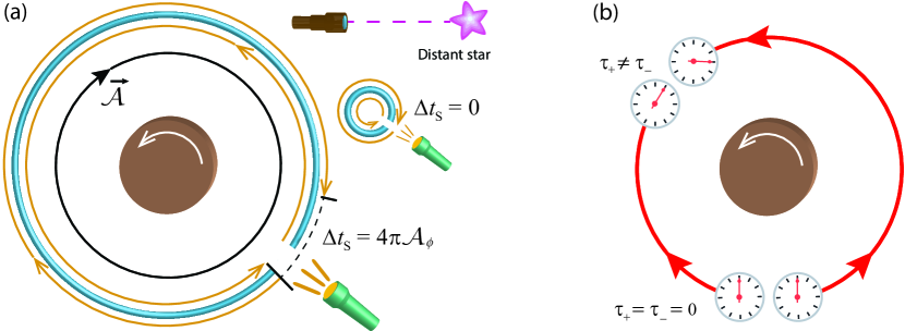
Figure 1: (a) Sagnac effect around spinning cylinders: a flashlight sends light beams propagating in opposite directions along optical fiber loops fixed with respect to the “distant stars” (i.e., to the asymptotic inertial frame at infinity). In each loop $C$, the difference in beam arrival times is $\Delta t_{{\rm S}}=2\oint_{C}\bm{\mathcal{A}}$; since $\bm{\mathcal{A}}$ is a closed form (${\bf d}\bm{\mathcal{A}}=0$), the effect vanishes for all loops not enclosing the cylinder, and has the same value (25) for all loops enclosing it (the co-rotating beam arriving first). (b) Frame independent gravitomagnetic clock effect: a pair of clocks in oppositely rotating circular geodesics around a cylinder; when the cylinder spins ($j\neq 0$) the clocks measure different proper times between the events where they meet, $\tau_{+}>\tau_{-}$.

$$\Delta t_{{\rm S}}=4\pi\mathcal{A}_{\phi}=-\frac{4\pi j}{1/4-\lambda_{{\rm m}}}$$ (25)

along any loop enclosing the cylinder, regardless of its shape; for instance, the large circular loop depicted in Fig. 1(a). It is worth noticing that this mirrors the situation for the Aharonov-Bohm effect around spinning charged cylinders, which is likewise independent of the shape of the paths; the two effects are actually described by formally analogous equations.

The apparatus above makes use of a star-fixed reference frame, which is physically realized by aiming telescopes at the distant stars[35, 36]. It is possible, however (still based on the Sagnac effect), to detect the cylinder’s rotation in a more local way, without the need for setting up a specific frame; only not with a single loop, as along a single loop the effect can always be made to vanish by spinning it with some angular velocity. In particular, for a concentric circular loop, the effect vanishes if it has zero angular momentum, i.e., if it comoves with the zero angular momentum observers (ZAMOs) of the same radius. The angular velocity of such observers, Eq. (69) of Ref. [5], is however $r$-dependent; hence, considering instead a “coil” of optical loops, as depicted in Fig. 4 of Ref. [5], provides a frame-independent (thought) experiment to detect the cylinder’s rotation, since it is impossible to make the effect vanish simultaneously in every loop when $j\neq 0\Leftrightarrow\text{$\bm{\mathcal{A}}$}\neq 0$.

4.4.1 Observer-independent gravitomagnetic clock effect

Another consequence of the vanishing of $\vec{H}$ is that the gravitomagnetic clock effect in Eq. (12) reduces to the Sagnac time delay, $\Delta t_{{\rm geo}}=\Delta t_{{\rm S}}=4\pi\mathcal{A}_{\phi}$; hence, all that was said above about beams in optical loops around the cylinder, applies as well to pairs of particles in oppositely rotating circular geodesics (the co-rotating geodesics having thus shorter periods). It is however actually possible to detect the cylinder’s rotation using only one pair of particles (i.e., a pair of clocks), through the difference in the proper times ($\tau_{+}$ and $\tau_{-}$) measured by each of them between the events where they meet, see Fig. 1 (b). From Eqs. (13) and (11), with $U_{\pm}^{0}=(-g_{00}-2\Omega_{{\rm geo}\pm}g_{0\phi}-\Omega_{{\rm geo}\pm}^{2}g_{\phi\phi})^{-1/2}$, we have

$$\Delta\tau\equiv\tau_{+}-\tau_{-}=\frac{8\pi jr^{2\lambda_{{\rm m}}}}{\sqrt{\alpha(1-4\lambda_{{\rm m}})(1-2\lambda_{{\rm m}})+8\lambda_{{\rm m}}j^{2}r^{8\lambda_{{\rm m}}-2}\alpha^{-1}(1/4-\lambda_{{\rm m}})^{-1}}}\ \ (>0)$$

(this result is mentioned in main paper [5], though without presenting it explicitly). Hence, when $j\neq 0$, the proper times measured by each clock differ when they meet, the co-rotating clock measuring a longer time.

4.5 Important limits: Levi-Civita static cylinder and cosmic strings

It is immediate to obtain important limits from the canonical form (21). Taking the limit $j\rightarrow 0$ yields the Levi-Civita metric[4, 2, 3]

$${\displaystyle{\displaystyle ds^{2}}=-\frac{r^{4\lambda_{{\rm m}}}}{\alpha}dt^{2}+r^{4\lambda_{{\rm m}}(2\lambda_{{\rm m}}-1)}(dr^{2}+dz^{2})}+\alpha r^{2(1-2\lambda_{{\rm m}})}d\phi^{2}\ .$$ (26)

The inertial fields $\vec{G}$ and $\vec{H}=0$, as well as the spatial metric $h_{ij}$, remain the same as in (21) (the same applying to the tidal fields/forces, see Sec. 5.2.3 in Ref. [5]). They differ only in the gravitomagnetic potential 1-form $\bm{\mathcal{A}}=-4j/(1-4\lambda_{{\rm m}})\mathbf{d}\phi$, governing global physical effects such as the Sagnac effect and synchronization gap (10) in loops around the cylinder, and the gravitomagnetic clock effect, which are all zero for the static metric (26), see Figs. 1-2.

The limit $\lambda_{{\rm m}}\rightarrow 0$ yields

$${\displaystyle{\displaystyle ds^{2}}=-\frac{1}{\alpha}\left[dt+4jd\phi\right]^{2}+dr^{2}+dz^{2}}+\alpha r^{2}d\phi^{2}$$ (27)

which is the metric of a spinning cosmic string[2, 37, 38] of Komar angular momentum per unit length $j$ and angle deficit $2\pi(1-\alpha^{1/2})\equiv 2\pi\delta$. In this case the spacetime is locally flat ($R_{\alpha\beta\gamma\delta}=0$) for $r\neq 0$. All the GEM inertial fields vanish, $\vec{G}=\vec{H}=0$ (and the same for the tidal fields), thus there are no gravitational forces of any kind. Global gravitational effects however subsist, governed by $\bm{\mathcal{A}}=-4j\mathbf{d}\phi$ and $\alpha$. The non-vanishing gravitomagnetic potential 1-form $\bm{\mathcal{A}}$ means that a Sagnac effect remains, thus the apparatuses manifesting the source’s rotation discussed in Sec. 4.4 apply here as well. The same applies to the synchronization of clocks: observers at rest in the coordinates of (27) (which are in this case inertial observers) can synchronize their clocks along closed loops not enclosing the string (i.e., the axis $r=0$), but are unable to do so for loops enclosing it. As for the gravitomagnetic clock effect, it does not apply here, as circular geodesics do not exist (since there is no gravitational attraction, $\vec{G}=0$). The angle deficit generates double images of objects located behind the string [39, 40], and a holonomy[41, 40] along closed (in spacetime or only spatially) loops around the string. Namely, vectors parallel transported along such loops turn out rotated by an angle $-2\pi\alpha^{1/2}$ (i.e, $2\pi\delta$) about the $z$-axis when they return to the initial position — an effect which is independent of the shape of the loop and of $j$; see Sec. 5.2.4 of Ref. [5]. One thus can say that the metric (27) possesses two holonomies: a spatial holonomy governed by $\alpha$, which is the same for spinning or non-spinning strings, plus a synchronization holonomy (Sec. 5.3.3 of Ref. [5]) that arises in the spinning case.

4.6 Summary of “canonical” features

We argue Eq. (21) to be the most natural, or canonical, form for the metric of a Weyl class rotating cylinder for the following reasons:

• the Killing vector field $\partial_{t}$ is (for $\alpha>0$) everywhere time-like (i.e., $g_{00}<0$ for all $r$), therefore physical observers $u^{\alpha}=(-g_{00})^{-1/2}\partial_{t}^{\alpha}$, at rest in the coordinates of (21), exist everywhere.

• The associated reference frame is asymptotically inertial, and thus fixed with respect to the “distant stars” (Sec. 4.4).

• A conserved Komar mass per unit length ($\lambda_{{\rm m}}$) can be defined from $\partial_{t}$ which matches its expected value from the gravitational field $\vec{G}$ and potential $\Phi$ in Sec. 4.4 (see also Sec. 5.2.1 of Ref. [5]), and also that of the Levi-Civita static cylinder (26).

• It is irreducibly given in terms of three parameters with a clear physical interpretation: the Komar mass ($\lambda_{{\rm m}}$) and angular momentum ($j$) per unit length, plus the parameter $\alpha$ governing the angle deficit of the spatial metric $h_{ij}$.

• The GEM fields are strikingly similar to the electromagnetic analogues — the electromagnetic fields of a rotating cylinder as measured in the inertial rest frame (namely $\bm{\mathcal{A}}=\mathcal{A}_{\phi}\mathbf{d}\phi$; $\mathcal{A}_{\phi}\equiv$constant, $\vec{H}=\mathbb{H}_{\alpha\beta}=0$, and $\Phi$ and $G_{,i}$ match the electromagnetic counterparts identifying the Komar mass per unit length $\lambda_{{\rm m}}$ with the minus charge per unit length $\lambda$, cf. Sec. 4 of Ref. [5]).

• It is immediate from it to obtain the two important limits: spinning cosmic string ($\lambda_{{\rm m}}=0$), and Levi-Civita static solution (evincing that $j=0$ is the necessary and sufficient condition).

• The GEM inertial fields and tidal tensors are the same as those of the Levi-Civita static cylinder (just like the electromagnetic forces produced by a charged spinning cylinder are the same as by a static one).

• It is obtained from a simple rigid rotation of coordinates, Eq. (15), which is a well-defined global coordinate transformation (Sec. 4.1).

• It makes immediately transparent the locally static but globally stationary nature of the metric (see Sec. 5 below).

• It has a smooth matching to the van Stockum interior solution (corresponding to a cylinder of rigidly rotating dust) written in star-fixed coordinates (Sec. 5.4.2 of Ref. [5]).

We conclude that the Lewis metric in its usual form (1)-(2) indeed possesses a trivial coordinate rotation [of angular velocity $-\Omega$, equivalently given by either of Eqs. (14)], which has apparently gone unnoticed in the literature, and causes the artificial features listed in Sec. 3. As shown in Sec. 5.4 of Ref. [5], such rotation has a simple interpretation when the solution is matched to the van Stockum interior solution (corresponding to a rigidly rotating cylinder of dust): the coordinate system in (1)-(2) is rigidly comoving with the cylinder.

5 Contrast with a locally (and globally) non-static solution — the Kerr spacetime

Question by O. Semerák: you were comparing the results for the (rotating) Weyl class Lewis metric with the static case; how about the comparison with Kerr, which is different because there the vorticity should contribute to the gravitomagnetic field?

The contrast with the Kerr spacetime is indeed instructive. In what pertains to gravitomagnetism, it fundamentally differs from the Weyl class cylindrical metrics (rotating or non-rotating) in two mains aspects: it is not locally static, and its Riemann tensor is not (except at the equatorial plane) “purely electric” [29].

Staticity.— a spacetime is static[42] within some region iff a time-like Killing vector field $\xi^{\alpha}$ exists which is proportional to the gradient of some (single-valued) function $\psi$, $\xi_{\alpha}=\eta\partial_{\alpha}\psi$. Locally, this condition is equivalent to the integral lines of $\xi^{\alpha}$ having no vorticity, i.e., being hypersurface orthogonal (globally, however, the vorticity-free condition is not sufficient [42, 43]). One can show (Proposition 5.1 in Ref. [5]) that, in the GEM framework, local staticity amounts to the existence of a coordinate system where the metric takes the stationary form (3) with $\bm{\mathcal{A}}$ closed ($\mathbf{d}\bm{\mathcal{A}}=0$); and global staticity to $\bm{\mathcal{A}}$ being moreover an exact form (in a globally well defined coordinate system).

The Weyl class Lewis metric (21) is locally static since $\mathbf{d}\bm{\mathcal{A}}=0$; but, unless $j=0\Rightarrow\bm{\mathcal{A}}=0$ (Levi-Civita static cylinder), not globally static, since $\bm{\mathcal{A}}=\mathcal{A}_{\phi}\mathbf{d}\phi$ is not an exact form. This means that the Killing vector field $\partial_{t}$ is hypersurface orthogonal but (unless $j=0$) such hypersurfaces are not of global simultaneity, see Fig. 2 (a)-(b). In the case of the Kerr spacetime, $\mathbf{d}\bm{\mathcal{A}}\neq 0$, so it is not globally static; no hypersurface orthogonal time-like Killing vector field exists, the only Killing vector field which is time-like at infinity being $\partial_{t}$ in Boyer-Lindquist coordinates, whose integral lines are well known to have vorticity. Geometrically, this means that the distribution of hyperplanes orthogonal to $\partial_{t}$ (i.e., the hyperplanes of local simultaneity[21], or local rest spaces of the “laboratory” observers) is not integrable, see Fig. 2 (c). On top of this, outside the equatorial plane, $R_{\alpha\beta\gamma\delta}$ is not purely electric (see Sec. V.C of Ref. [29]), thus no observers exist measuring a vanishing gravitomagnetic tidal tensor $\mathbb{H}_{\alpha\beta}$.

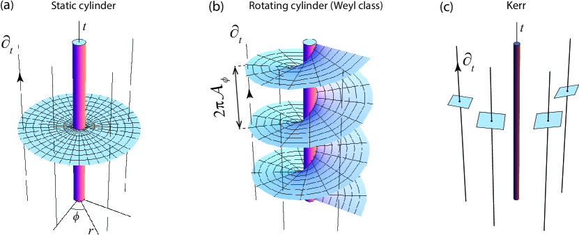
Figure 2: (a)-(b): In the Weyl class Lewis metrics (21) the Killing vector field $\partial_{t}$ is hypersurface orthogonal; such hypersurface is of global simultaneity (a plane, in a $t,r,\phi$ plot) for a non-spinning (Levi-Civita) cylinder, and of local but non-global simultaneity (the helicoid $t-\mathcal{A}_{\phi}\phi=const.$) in the spinning case. (c) In the Kerr spacetime $\partial_{t}$ is not hypersurface orthogonal, i.e., the distribution of hyperplanes orthogonal to $\partial_{t}$ (hyperplanes of local simultaneity) is not integrable. In (a) observers of worldlines tangent to $\partial_{t}$ (“laboratory observers”) are able to globally synchronize their clocks. In (b) they are unable to synchronize their clocks around the cylinder: each $2\pi$ turn along the helicoid leads to a different event in time, the jump between turns being the synchronization gap $\Delta t_{{\rm sync}}=2\pi\mathcal{A}_{\phi}$. In (c) the laboratory observers are (generically) unable to synchronize their clocks along any spatially closed loop, $\Delta t_{{\rm sync}}=\oint\bm{\mathcal{A}}\neq 0$.

Physically, this means that whereas for the Weyl class spinning cylinder (21) only the first level of gravitomagnetism in Table 1 is non-zero, in the Kerr spacetime all the three levels are non-zero. Therein it is thus possible to detect the source’s rotation in a more local way (i.e., not needing experiments on loops around the source): in a reference frame fixed to the distant stars, due to the non-zero gravitomagnetic field $\vec{H}$, test particles in geodesic motion will appear to be deflected by a gravitomagnetic (or Coriolis) force $\gamma\vec{U}\times\vec{H}$, cf. Eq. (4), causing e.g. their orbits to precess (Lense-Thirring precession[35]), and gyroscopes will as well be seen to precess, cf. Eq. (6). The non-vanishing $\mathbb{H}_{\alpha\beta}$ means moreover that gyroscopes at rest (or generically moving) will be acted by a force (7).

Level of Gravitomagnetism		Lewis-Weyl	Kerr
Governing object	Physical effect
$\vec{\mathcal{A}}$ (gravitomagnetic vector potential)	$\bullet$ Sagnac effect $\bullet$ Synchronization gap	$\checkmark$ (global effects)	$\checkmark$ (global and local)
$\vec{H}$ (gravitomagnetic field $=e^{\phi}\nabla\times\vec{\mathcal{A}}$)	$\bullet$ gravitomagnetic force    $m\gamma\vec{U}\times\vec{H}$ $\bullet$ gyroscope precession    $d\vec{S}/d\tau=\vec{S}\times\vec{H}/2$ $\bullet$ local Sagnac effect in    light gyroscope	$\times$	$\checkmark$
$\vec{H}+\vec{\mathcal{A}}$	$\bullet$ Gravitomagnetic     “clock” effect	$\bullet$ co-rotating geodesic    has shorter period	$\bullet$ co-rotating geodesic    has longer period
$\mathbb{H}_{\alpha\beta}$ (gravitomag. tidal tensor $\sim\partial_{i}\partial_{j}\mathcal{A}_{k}$)	$\bullet$ Force on gyroscope    ${\displaystyle DP^{\alpha}/d\tau=-\mathbb{H}^{\beta\alpha}S_{\beta}}$	$\times$	$\checkmark$

Table 1: Gravitomagnetic effects present in the Weyl class Lewis metric, and in the Kerr spacetime, as measured in star-fixed reference frames (“canonical” and Boyer-Lindquist coordinate systems, respectively), split by levels of gravitomagnetism, corresponding to orders of differentiation of $\bm{\mathcal{A}}$.

Even in what pertains to the first level of gravitomagnetism (governed by $\bm{\mathcal{A}}$), present in both, they substantially differ. The fact that $\mathbf{d}\bm{\mathcal{A}}=0$ in the Lewis-Weyl metric means that a Sagnac effect (9) arises only on loops enclosing the cylinder (as discussed in Sec. 4.4), and is independent of the shape of the loop; and similarly for the synchronization of clocks: the laboratory observers are able to synchronize their clocks along spatially closed loops that do not enclose the cylinder [in other words, closed in spacetime synchronization curves exist along the helicoid of Fig. 2 (b)]; it is only on loops around the cylinder that a synchronization gap (10) arises, see Fig. 2 (b). In the Kerr spacetime, by contrast, since $\mathbf{d}\bm{\mathcal{A}}\neq 0$, the Sagnac effect depends on the shape of the loop, and is generically non-zero (regardless of the loop enclosing or not the axis). The laboratory observers are likewise unable to synchronize their clocks around generic closed loops.

Another interesting contrast is in the gravitomagnetic clock effect (12). Around the spinning cylinder (21), since $\vec{H}=0$, it reduces to the Sagnac time-delay (25), and thus the co-rotating geodesic has a shorter period. In the case of the Kerr spacetime, by contrast, the term $\Delta t_{H}$ of (12) is not zero,

$$\Delta t_{{\rm geo}}=\Delta t_{{\rm S}}+\Delta t_{H}=4\pi\frac{J}{M};\qquad\Delta t_{{\rm S}}=-\frac{8\pi J}{r-2M}\,(<0);\qquad\Delta t_{H}=\frac{4\pi Jr}{M(r-2M)}\,(>0),$$

and is actually dominant [27], so it is the other way around: the co-rotating orbit has a longer period, $\Delta t_{{\rm geo}}=4\pi J/M>0$. The physical interpretation of $\Delta t_{H}>0$ is that the gravitomagnetic force $\gamma\vec{U}\times\vec{H}$ in Eq. (4) is repulsive (attractive) for co- (counter-) rotating geodesics, see Fig. 1(b) of Ref. [27].

References

- [1] T. Lewis, “Some special solutions to the equations of axially symmetric gravitational fields,” Proc. Roy. Soc. Lond. A136 (1932) 179–192.
- [2] M. F. A. da Silva, L. Herrera, F. M. Paiva, and N. O. Santos, “The parameters of the Lewis metric for the Weyl class,” General Relativity and Gravitation 27 no. 8, (Aug, 1995) 859–872.
- [3] M. F. A. da Silva, L. Herrera, F. M. Paiva, and N. O. Santos, “On the parameters of Lewis metric for the Lewis class,” Class. Quant. Grav. 12 (1995) 111–118, arXiv:gr-qc/9607057.
- [4] J. B. Griffiths and J. Podolsky, Exact Space-Times in Einstein’s General Relativity. Cambridge Monographs on Mathematical Physics. Cambridge University Press, Cambridge, 2009.
- [5] L. F. O. Costa, J. Natário, and N. O. Santos, “Gravitomagnetism in the Lewis cylindrical metrics,” Class. Quant. Grav. 38 no. 5, (2021) 055003, arXiv:1912.09407.
- [6] W. J. van Stockum, “IX. The Gravitational Field of a Distribution of Particles Rotating about an Axis of Symmetry,” Proceedings of the Royal Society of Edinburgh 57 (1938) 135–154.
- [7] “Gravitomagnetism in the Lewis cylindrical metrics,” Invited talk at the parallel session PT5 – “Dragging is never draggy: MAss and CHarge flows in GR", sixteenth Marcel Grossmann Meeting (MG16), July 5-10 2021 . https://youtu.be/ho31IgLNxu8.
- [8] L. D. Landau and E. M. Lifshitz, The classical theory of fields; 4rd ed., vol. 2 of Course of theoretical physics. Butterworth-Heinemann, Oxford, UK, 1975. Trans. from the Russian.
- [9] D. Lynden-Bell and M. Nouri-Zonoz, “Classical monopoles: Newton, NUT space, gravomagnetic lensing, and atomic spectra,” Rev. Mod. Phys. 70 (Apr, 1998) 427–445.
- [10] R. T. Jantzen, P. Carini, and D. Bini, “The Many faces of gravitoelectromagnetism,” Annals Phys. 215 (1992) 1–50, arXiv:gr-qc/0106043.
- [11] L. F. O. Costa and J. Natário, “Gravito-electromagnetic analogies,” General Relativity and Gravitation 46 no. 10, (2014) 1792, arXiv:1207.0465.
- [12] M. Mathisson, “Neue mechanik materieller systemes,” Acta Phys. Polon. 6 (1937) 163. [Gen. Relativ. Gravit. 42, 1011 (2010)].
- [13] A. Papapetrou, “Spinning test particles in general relativity. 1.,” Proc. Roy. Soc. Lond. A209 (1951) 248–258.
- [14] L. F. O. Costa, J. Natário, and M. Zilhão, “Spacetime dynamics of spinning particles: Exact electromagnetic analogies,” Phys. Rev. D 93 no. 10, (2016) 104006, arXiv:1207.0470.
- [15] W. G. Dixon, “A covariant multipole formalism for extended test bodies in general relativity,” Il Nuovo Cimento 34 (1964) 317.
- [16] Y. Aharonov and D. Bohm, “Significance of electromagnetic potentials in the quantum theory,” Phys. Rev. 115 (Aug, 1959) 485–491.
- [17] E. J. Post, “Sagnac effect,” Rev. Mod. Phys. 39 (Apr, 1967) 475–493.
- [18] E. Kajari, M. Buser, C. Feiler, and W. P. Schleich, “Rotation in relativity and the propagation of light,” in Proceedings of the International School of Physics "Enrico Fermi", Course CLXVIII, pp. 45–148 [Riv. Nuovo Cim. 32, 339–438]. IOS Press, Amsterdam, 2009. arXiv:0905.0765.
- [19] A. Ashtekar and A. Magnon, “The Sagnac effect in general relativity,” J. Math. Phys. 16 (1975) 341–344.
- [20] A. Tartaglia, “General relativistic corrections to the Sagnac effect,” Phys. Rev. D 58 (1998) 064009, arXiv:gr-qc/9806019.
- [21] E. Minguzzi, “Simultaneity and generalized connections in general relativity,” Class. Quant. Grav. 20 (2003) 2443–2456, arXiv:gr-qc/0204063.
- [22] M. L. Ruggiero, “Sagnac Effect, Ring Lasers and Terrestrial Tests of Gravity,” Galaxies 3 no. 2, (2015) 84–102, arXiv:1505.01268.
- [23] J. Cohen and B. Mashhoon, “Standard clocks, interferometry, and gravitomagnetism,” Physics Letters A 181 (1993) 353 – 358.
- [24] W. B. Bonnor and B. R. Steadman, “The gravitomagnetic clock effect,” Classical and Quantum Gravity 16 no. 6, (1999) 1853.
- [25] D. Bini, R. T. Jantzen, and B. Mashhoon, “Gravitomagnetism and relative observer clock effects,” Class. Quant. Grav. 18 (2001) 653–670, arXiv:gr-qc/0012065.
- [26] L. Iorio, H. I. M. Lichtenegger, and B. Mashhoon, “An Alternative derivation of the gravitomagnetic clock effect,” Class. Quant. Grav. 19 (2002) 39–49, arXiv:gr-qc/0107002.
- [27] L. F. O. Costa and J. Natário, “Frame-Dragging: Meaning, Myths, and Misconceptions,” Universe 7 no. 10, (2021) 388, arXiv:arXiv:2109.14641.
- [28] A. Tartaglia, “Detection of the gravitomagnetic clock effect,” Class. Quant. Grav. 17 (2000) 783–792, arXiv:gr-qc/9909006.
- [29] L. F. O. Costa, L. Wylleman, and J. Natário, “Gravitomagnetism and the significance of the curvature scalar invariants,” Phys. Rev. D 104 (2021) 084081, arXiv:1603.03143.
- [30] C. B. G. McIntosh, R. Arianrhod, S. T. Wade, and C. Hoenselaers, “Electric and magnetic Weyl tensors: classification and analysis,” Classical and Quantum Gravity 11 (Jun, 1994) 1555–1564.
- [31] W. B. Bonnor, “Solution of Einstein’s equations for a line-mass of perfect fluid,” Journal of Physics A: Mathematical and General 12 no. 6, (1979) 847–851.
- [32] W. Israel, “Line sources in general relativity,” Phys. Rev. D 15 (Feb, 1977) 935–941.
- [33] L. Marder, “Gravitational Waves in General Relativity. I. Cylindrical Waves,” Proceedings of the Royal Society of London Series A 244 (1958) 524–537.
- [34] D. Lynden-Bell and J. Bičák, “Komar fluxes of circularly polarized light beams and cylindrical metrics,” Phys. Rev. D 96 no. 10, (2017) 104053, arXiv:1712.06980.
- [35] I. Ciufolini and J. A. Wheeler, Gravitation and Inertia. Princeton Series in Physics, Princeton, NJ, 1995.
- [36] I. Ciufolini, “Dragging of inertial frames,” Nature 449 (2007) 41–47.
- [37] A. Barros, V. B. Bezerra, and C. Romero, “Global aspects of gravitomagnetism,” Mod. Phys. Lett. A18 (2003) 2673–2679, arXiv:gr-qc/0307062.
- [38] B. Jensen and H. H. Soleng, “General-relativistic model of a spinning cosmic string,” Phys. Rev. D 45 (May, 1992) 3528–3533.
- [39] M. Hindmarsh and T. Kibble, “Cosmic strings,” Rept. Prog. Phys. 58 (1995) 477–562, arXiv:hep-ph/9411342.
- [40] L. H. Ford and A. Vilenkin, “A gravitational analogue of the Aharonov-Bohm effect,” Journal of Physics A: Mathematical and General 14 (1981) 2353–2357.
- [41] M. Nouri-Zonoz and A. Parvizi, “Gaussian curvature and global effects: Gravitational Aharonov-Bohm effect revisited,” Phys. Rev. D 88 no. 2, (2013) 023004, arXiv:1306.1883.
- [42] J. Stachel, “Globally stationary but locally static space-times: A gravitational analog of the Aharonov-Bohm effect,” Phys. Rev. D 26 (1982) 1281–1290.
- [43] W. B. Bonnor, “The rigidly rotating relativistic dust cylinder,” Journal of Physics A: Mathematical and General 13 (1980) 2121.