Data-driven integration of norm-penalized mean-variance portfolios

Abstract

Mean-variance optimization (MVO) is known to be sensitive to estimation error in its inputs. Norm penalization of MVO programs is a regularization technique that can mitigate the adverse effects of estimation error. We augment the standard MVO program with a convex combination of parameterized $L_{1}$ and $L_{2}$-norm penalty functions. The resulting program is a parameterized quadratic program (QP) whose dual is a box-constrained QP. We make use of recent advances in neural network architecture for differentiable QPs and present a data-driven framework for optimizing parameterized norm-penalties to minimize the downstream MVO objective. We present a novel technique for computing the derivative of the optimal primal solution with respect to the parameterized $L_{1}$-norm penalty by implicit differentiation of the dual program. The primal solution is then recovered from the optimal dual variables. Historical simulations using US stocks and global futures data demonstrate the benefit of the data-driven optimization approach.

Keywords: Data-driven optimization, differentiable quadratic programming, mean-variance optimization

1 Introduction

The Markowitz (1952) mean-variance optimization (MVO) requires as input estimates of asset mean returns and covariances. Asset returns, however, are nonstationary and exhibit statistically insignificant auto-correlation (Drees and Starica, 2002; Engle, 1982; Starica and Granger, 2005) and are therefore estimated with a high degree of uncertainty Michaud and Michaud (2008b). Moreover, estimating a covariance matrix of $N$ assets requires computing $N(N+1)/2$ cross-covariance terms and therefore when the number of assets is large relative to the relevant number of historical observations then the estimated covariance matrix can be numerically unstable (Ledoit and Wolf, 2004a). As such, the sample covariance matrix and the action of its inverse is also contaminated with estimation error (Jobson and Korkie, 1980).

In this paper, we address the adverse effects of estimation error by augmenting the mean-variance objective with a norm-penalty on portfolio weights. We follow the work of Ho et al. (2015) and consider a convex combinations of general $L_{1}$ and $L_{2}$-norm penalty functions, presented below.

$$P(\operatorname{\bf z})=\alpha\operatorname{\bm{\gamma}}_{1}\lVert\operatorname{\bf E}(\operatorname{\bm{\theta}}_{1})\operatorname{\bf z}\rVert_{1}+(1-\alpha)\frac{\operatorname{\bm{\gamma}}_{2}}{2}\lVert\operatorname{\bf D}(\operatorname{\bm{\theta}}_{2})\operatorname{\bf z}\rVert_{2}^{2}.$$ (1)

Here, $\operatorname{\bf E}(\operatorname{\bm{\theta}}_{1})$ and $\operatorname{\bf D}(\operatorname{\bm{\theta}}_{2})$ are parameterized sparsifying and regularization transforms and therefore Equation $\eqref{eq:penalty_1}$ generalizes the standard elastic net formulation (Zou and Hastie, 2005). The choice of the generalized elastic net penalty is deliberate and motivated by prior work that establishes the connection between norm-penalized portfolio weights with covariance shrinkage and robust optimization (DeMiguel et al., 2009).

Determining the penalty parameters, $(\operatorname{\bm{\theta}}_{1},\operatorname{\bm{\theta}}_{2},\operatorname{\bm{\gamma}}_{1},\operatorname{\bm{\gamma}}_{2})$, is generally difficult. Traditionally, the penalty structures, $\operatorname{\bf E}(\operatorname{\bm{\theta}}_{1})$ and $\operatorname{\bf D}(\operatorname{\bm{\theta}}_{2})$, are specified in advanced by the user and the amount of penalization, $(\operatorname{\bm{\gamma}}_{1},\operatorname{\bm{\gamma}}_{2})$, is then estimated by cross-validation (DeMiguel et al., 2009; Elmachtoub and Grigas, 2017; Hastie et al., 2001). Recently, Butler and Kwon (2021b, c) present a parameter estimation approach that optimizes prediction model parameters to directly minimize downstream portfolio objectives. Indeed, more generally there is a growing body of research on the efficacy of integrated prediction and decision optimization modelling (see for example Amos et al. (2019); Donti et al. (2017); Bertsimas and Kallus (2020); Elmachtoub and Grigas (2017); Elmachtoub et al. (2020); Grigas et al. (2021); Mandi and Guns (2020)).

Motivated by the aforementioned work, in this paper we present an end-to-end framework for optimizing the penalty parameters of Equation $\eqref{eq:penalty_1}$ such that the resulting norm-penalized MVO program induces optimal portfolio decision-making. We structure the parameter estimation problem as an end-to-end neural network with differentiable QP layers and present a novel technique for computing the derivative of the optimal primal solution with respect to the parameterized $L_{1}$-norm penalty by implicit differentiation of the dual program. An advantage of our approach is that the penalty structure does need not be fully-specified in advance and instead penalty parameters are optimized in a data-driven manner. To our knowledge, our framework is the first to consider the optimization of parameterized norm-penalty structures in a portfolio optimization setting. The remainder of the paper is outlined as follows. We begin with a review of the relevant literature in the field of robust and norm-penalized portfolio optimization. In Section 2 we present the optimization framework for learning parameterized quadratic programs (QPs). We demonstrate that the dual of the norm-penalized QP is a box-constrained QP and provide a first-order gradient descent approach for optimizing the penalty parameters by backpropagating through differentiable QP layers (Amos and Kolter, 2017; Butler and Kwon, 2021a). We conclude with a simulation study using both US stocks and global futures data and demonstrate the flexibility and effectiveness of the approach. We find that the parameterized norm-penalized MVO portfolios, in which the exact penalty structure is learned from the data, result in improved out-of-sample portfolio objectives.

1.1 Relevant literature:

MVO portfolios are known to be sensitive to estimation error and thus frameworks for mitigating the adverse effects of estimation error are fundamental to the successful application of modern portfolio theory (Chopra and Ziemba, 1993; Jobson and Korkie, 1982; Michaud and Michaud, 2008b). For example, Black and Litterman (1991) present a Bayesian framework for altering MVO inputs based on prior estimates of means and covariances. Alternatively, Michaud and Michaud (2008a) propose a resampled MVO process that averages the optimal weights derived from multiple resampled realizations of asset returns. However, the estimates assume a multivariate normal distribution, with moments equal to the in-sample estimates and the impact of sampling error is assumed to be in proportion to the variance of the sample mean.

Ledoit and Wolf (2004b, 2012), demonstrate that when the covariance matrix is poorly conditioned the portfolio construction process can become unstable, resulting in concentrated ‘error-maximizing’ portfolio weights. Their methods focus on providing improved covariance estimates based on James-Stein shrinkage (Stein, 1956). They propose covariance estimates that are a weighted average of the sample covariance estimate and a structured covariance matrix. The ‘optimal’ amount of shrinkage is then determined by minimizing the mean squared error of the estimate to the realized covariance.

Most closely related to our work, DeMiguel et al. (2009) and Ho et al. (2015) mitigate ‘error-maximization’ by augmenting MVO portfolios with $L_{1}$ and $L_{2}$-norm penalties on portfolio weights. They demonstrate that their norm-penalty formulations are equivalent to a robust MVO counterpart and propose tuning the penalty parameters by bootstrapping the historical distribution. More generally, robust optimization insulates against estimation error by minimizing objectives under worst-case realizations of the estimates (Goldfarb and Iyengar, 2003). The success of robust optimization typical depends on properly defining and calibrating the uncertainty structure and in general poorly calibrated uncertainty structures will result in overly conservative or intractable programs (Bertsimas et al., 2014).

While the seminal work in the field of robust optimization provides several theoretical methods for constructing good uncertainty sets (Ben-Tal et al., 2009; Ben-Tal and Nemirovski, 2000; Bertsimas and Sim, 2004; Goldfarb and Iyengar, 2003), in quantitative finance, defining appropriate uncertainty structures remains a relatively ad-hoc process. For example, Goldfarb and Iyengar (2003) propose calibrating the uncertainty structure for both the mean and covariance by considering the covariances estimates from a linear regression model and cast the robust counterpart as a convex second-order cone program. Tutuncu and Koenig (2004) consider a robust MVO counterpart with box uncertainty sets and calibrate the uncertainty bounds by bootstrapping the historical return distribution. Zhu et al. (2009) consider robust MVO under ellipsoidal uncertainty and demonstrate that when the uncertainty matrix is proportional to the asset covariance matrix then the robust MVO counterpart is equivalent to a nominal MVO with a larger risk aversion parameter. More recently, Yin et al. (2019) argue for the use of ellipsoidal uncertainty sets instead of the more restrictive box uncertainty sets and propose calibrating the level of uncertainty in proportion to asset Sharpe ratios.

In all cases discussed above we find that the regularization structures are determined in advance by the user and then the desired amount of regularization is estimated independently from the downstream portfolio optimization. In this paper, the portfolio regularization structure takes the form of parameterized norm-penalties on portfolio weights. In contrast to prior work, however, we present an end-to-end framework for optimizing parameterized norm-penalties in order to directly minimize the downstream portfolio optimization objective. Our parameterized norm-penalty optimization solution is motivated by recent work that advocates for the use of neural networks to optimize model hyper-parameters in settings where an exhaustive parameter search would be computationally impractical (see for example Feng and Simon (2017); Ichnowski et al. (2021); Lorraine and Duvenaud (2018); Pedregosa (2016)). The proposed framework is flexible and obviates the need to pre-define a specific norm-penalty structure and instead enables users to formulate parameterized models that are fit to a training dataset in a systematic and data-driven manner. Indeed, previous work considers the integration of prediction modelling with downstream portfolio optimization using an end-to-end neural network approach (Butler and Kwon, 2021b, c; Chevalier et al., 2022; Uysal et al., 2021). In all cases, however, the optimal portfolios are determined by differentiable optimization layers that directly compute the optimal primal solutions. However, forward solving and backpropagating through an $L_{1}$-norm penalized QP is challenging and is currently not supported by existing QP layer architectures. In this paper we present an alternative neural network architecture for $L_{1}$-norm penalized QPs that instead solves the dual program - a box-constrained QP - and then recovers the primal solution from the optimal dual variables. To our knowledge, our end-to-end neural network is the first to consider implicit differentiation of the dual of an $L_{1}$-norm penalized QP and thus advances the understanding and implementation of differentiable optimization layers for solving non-smooth optimization programs.

2 Methodology

We follow closely to the methodology as described in Butler and Kwon (2021c). We denote the matrix of (excess) return observations as ${\operatorname{\bf Y}=[\operatorname{\bf y}^{(1)},\operatorname{\bf y}^{(2)},...,\operatorname{\bf y}^{(m)}]\in\mathbb{R}^{d_{z}\times m}}$ and let $\operatorname{\bf z}\in\mathbb{R}^{d_{z}}$ denote the vector of portfolio weights. The mean-variance optimal portfolio at time $i$ is given by:

$$\begin{split}\operatorname*{minimize}_{z}\quad&-\operatorname{\bf z}^{T}\mathop{\mathrm{\operatorname{\bf y}}^{(i)}}+\frac{\delta}{2}\operatorname{\bf z}^{T}\mathop{\mathrm{\operatorname{\bf V}}^{(i)}}\operatorname{\bf z}\\ \text{subject to}\quad&\operatorname{\bf A}\operatorname{\bf z}=\operatorname{\bf b},\qquad\operatorname{\bf G}\operatorname{\bf z}\leq\operatorname{\bf h}\\ \end{split}$$ (2)

with risk-aversion parameter $\delta\in\mathbb{R}_{+}$ and time-varying symmetric positive definite covariance matrix $\mathop{\mathrm{\operatorname{\bf V}}^{(i)}}\in\mathbb{R}^{d_{z}\times d_{z}}$. The linear equality and inequality constraints are described by matrices $\operatorname{\bf A}\in\mathbb{R}^{d_{\text{eq}}\times d_{z}}$, $\operatorname{\bf b}\in\mathbb{R}^{d_{\text{eq}}}$ and $\operatorname{\bf G}\in\mathbb{R}^{d_{\text{iq}}\times d_{z}}$, $\operatorname{\bf h}\in\mathbb{R}^{d_{\text{iq}}}$, respectively.

At decision time, $i-1$, however, the realization of asset returns, $\mathop{\mathrm{\operatorname{\bf y}}^{(i)}}$, is unobservable. Instead, associated feature variables, $\mathop{\mathrm{\operatorname{\bf x}}^{(i)}}\in\mathbb{R}^{d_{x}}$, are used to estimate $\mathop{\mathrm{\operatorname{\bf y}}^{(i)}}$. We consider linear regression models of the form:

$$\mathop{\mathrm{\hat{\operatorname{\bf y}}}^{(i)}}=\hat{\operatorname{\bm{\beta}}}^{T}\mathop{\mathrm{\operatorname{\bf x}}^{(i)}}$$

where $\hat{\operatorname{\bm{\beta}}}\in\mathbb{R}^{d_{x}\times d_{y}}$ denotes the matrix of regression coefficients. Let ${\ell(\hat{\operatorname{\bf y}},\operatorname{\bf y})=\lVert\hat{\operatorname{\bf y}}-\operatorname{\bf y}\rVert_{2}^{2}}$ denote the least-squares loss function. Therefore, given a training data set $\mathcal{D}=\{(\mathop{\mathrm{\operatorname{\bf x}}^{(i)}},\mathop{\mathrm{\operatorname{\bf y}}^{(i)}})\}_{i=1}^{m}$, we estimate $\hat{\operatorname{\bm{\beta}}}$ by solving:

$$\begin{split}\hat{\operatorname{\bm{\beta}}}&=\operatorname*{argmin}_{\operatorname{\bm{\beta}}}\mathbb{E}_{D}[\ell(\operatorname{\bm{\beta}}^{T}\mathop{\mathrm{\operatorname{\bf x}}^{(i)}},\mathop{\mathrm{\operatorname{\bf y}}^{(i)}})],\end{split}$$ (3)

where $\mathbb{E}_{\mathcal{D}}$ denotes the expectation with respect to the training distribution $\mathcal{D}$. Following Butler and Kwon (2021b), the least-squares estimates of asset mean returns and covariances are given by:

$$\begin{split}\mathop{\mathrm{\hat{\operatorname{\bf y}}}^{(i)}}&=\hat{\operatorname{\bm{\beta}}}^{T}\mathop{\mathrm{\operatorname{\bf x}}^{(i)}}\\ \mathop{\mathrm{\hat{\operatorname{\bf V}}}^{(i)}}&=\hat{\operatorname{\bm{\beta}}}^{T}\mathop{\mathrm{\hat{\operatorname{\bf W}}}^{(i)}}\hat{\operatorname{\bm{\beta}}}+\mathop{\mathrm{\hat{\operatorname{\bf F}}}^{(i)}},\end{split}$$ (4)

where $\mathop{\mathrm{\hat{\operatorname{\bf W}}}^{(i)}}$ denotes the time-varying feature covariance matrix and $\mathop{\mathrm{\hat{\operatorname{\bf F}}}^{(i)}}$ denotes the diagonal matrix of residual variances.

Using the estimates, $\mathop{\mathrm{\hat{\operatorname{\bf y}}}^{(i)}}$ and $\mathop{\mathrm{\hat{\operatorname{\bf V}}}^{(i)}}$, we can solve the nominal MVO portfolio using information available at time $i-1$:

$$\begin{split}\operatorname*{minimize}_{z}\quad&-\operatorname{\bf z}^{T}\mathop{\mathrm{\hat{\operatorname{\bf y}}}^{(i)}}+\frac{\delta}{2}\operatorname{\bf z}^{T}\mathop{\mathrm{\hat{\operatorname{\bf V}}}^{(i)}}\operatorname{\bf z}\\ \text{subject to}\quad&\operatorname{\bf A}\operatorname{\bf z}=\operatorname{\bf b},\qquad\operatorname{\bf G}\operatorname{\bf z}\leq\operatorname{\bf h}.\\ \end{split}$$ (5)

We denote the optimal MVO portfolio weights as $\mathop{\mathrm{\operatorname{\bf z}^{*}}^{(i)}}$. We reiterate that Program $\eqref{eq:mvo_ineq}$ assumes that asset means and covariances are known with certainty, whereas Program $\eqref{eq:mvo_ineq_est}$ is formed at time $i-1$ using the estimates of mean returns and covariances.

In reality all prediction models do make some error (i.e. $\mathop{\mathrm{\hat{\operatorname{\bf y}}}^{(i)}}\neq\mathop{\mathrm{\operatorname{\bf y}}^{(i)}}$, $\mathop{\mathrm{\hat{\operatorname{\bf V}}}^{(i)}}\neq\mathop{\mathrm{\operatorname{\bf V}}^{(i)}}$). In this paper we address the adverse effects of estimation error by augmenting the nominal MVO program with norm-penalties on portfolio weights:

$$\begin{split}\operatorname*{minimize}_{z}\quad&c_{P}(\operatorname{\bf z})=-\operatorname{\bf z}^{T}\mathop{\mathrm{\hat{\operatorname{\bf y}}}^{(i)}}+\frac{\delta}{2}\operatorname{\bf z}^{T}\mathop{\mathrm{\operatorname{\bf V}}^{(i)}}\operatorname{\bf z}+\alpha\operatorname{\bm{\gamma}}_{1}\lVert\operatorname{\bf E}(\operatorname{\bm{\theta}}_{1})\operatorname{\bf z}\rVert_{1}+(1-\alpha)\frac{\operatorname{\bm{\gamma}}_{2}}{2}\lVert\operatorname{\bf D}(\operatorname{\bm{\theta}}_{2})\operatorname{\bf z}\rVert_{2}^{2}\\ \text{subject to}\quad&\operatorname{\bf A}\operatorname{\bf z}=\operatorname{\bf b},\quad\operatorname{\bf G}\operatorname{\bf z}\leq\operatorname{\bf h}.\end{split}$$ (6)

Here $\lVert\cdot\rVert_{p}$ denotes the standard $L_{p}$-norm and $0\leq\alpha\leq 1$. The matrices, $\operatorname{\bf E}(\operatorname{\bm{\theta}}_{1})\in\mathbb{R}^{d_{\text{E}}\times d_{z}}$ and ${\operatorname{\bf D}(\operatorname{\bm{\theta}}_{2})\in\mathbb{R}^{d_{\text{D}}\times d_{z}}}$ are parameterized sparsifying and regularization transforms, respectively. Observe, that when $\alpha=1$ and $\operatorname{\bf E}(\operatorname{\bm{\theta}}_{1})=\operatorname{\bf I}$ then the penalty is the standard $L_{1}$-norm penalty common to many applications in statistics and engineering (Tibshirani, 1996; Kim et al., 2008). Conversely, when $\alpha=0$ and $\operatorname{\bf D}(\operatorname{\bm{\theta}}_{2})=\operatorname{\bf I}$ then the penalty is the standard $L_{2}$-norm penalty or Tikhonov regularization for approximations to ill-posed problems (Tikhonov, 1963). In its general form the norm-penalty resembles a generalization of the elastic net penalty for joint regularization and feature selection in least-squares regression (Zou and Hastie, 2005). As mentioned earlier, the choice of this specific norm-penalty is deliberate and motivated by prior work that establishes the connection between norm-penalized portfolio weights with covariance shrinkage and robust optimization.

The primary technical challenge is in optimizing the norm-penalty parameters such that the norm-penalized MVO portfolio induces optimal portfolio decisions. As described in Section 1.1, a traditional approach would pre-specify the norm-penalty structures, $\operatorname{\bf E}(\operatorname{\bm{\theta}}_{1})$ and $\operatorname{\bf D}(\operatorname{\bm{\theta}}_{2})$, and the optimal amount of penalization, $(\operatorname{\bm{\gamma}}_{1},\operatorname{\bm{\gamma}}_{2})$, is then estimated independently from its use in the downstream portfolio optimization. In contrast, in the following subsection we present an end-to-end framework for optimizing parameterized norm-penalties with the aim of inducing optimal MVO portfolio decision-making.

2.1 Optimization framework

Let $c\colon\mathbb{R}^{d_{z}\times m}\times\mathbb{R}^{d_{z}\times m}\rightarrow\mathbb{R}$ denote the realized portfolio objective (cost) function, which takes as input the optimal decisions: $\{\mathop{\mathrm{\operatorname{\bf z}^{*}}^{(i)}}\}_{i=1}^{m}$ and realized returns: $\{{\mathop{\mathrm{\operatorname{\bf y}}^{(i)}}}\}_{i=1}^{m}$. Specifically, in this paper we consider the minimum-variance, $c_{\text{MV}}$, and maximum Sharpe ratio, $c_{\text{SR}}$, costs, presented below:

$$c_{\text{MV}}(\{\mathop{\mathrm{\operatorname{\bf z}^{*}}^{(i)}}\}_{i=1}^{m},\{{\mathop{\mathrm{\operatorname{\bf y}}^{(i)}}}\}_{i=1}^{m})=\sigma^{2}\quad\text{and}\quad c_{\text{SR}}(\{\mathop{\mathrm{\operatorname{\bf z}^{*}}^{(i)}}\}_{i=1}^{m},\{{\mathop{\mathrm{\operatorname{\bf y}}^{(i)}}}\}_{i=1}^{m})=-\frac{\mu-r_{f}}{\sigma}$$ (7)

where $r_{f}$ denotes the risk-free rate and:

$$\mu=\frac{1}{m}\sum_{i=1}^{m}\mathop{\mathrm{\operatorname{\bf z}^{*}}^{{T}^{(i)}}}\mathop{\mathrm{\operatorname{\bf y}}^{(i)}}\quad\text{and}\quad\sigma^{2}=\frac{1}{m}\sum_{i=1}^{m}(\mathop{\mathrm{\operatorname{\bf z}^{*}}^{{T}^{(i)}}}\mathop{\mathrm{\operatorname{\bf y}}^{(i)}}-\mu)^{2}.$$

We seek to optimize the penalty parameters, $\operatorname{\bm{\theta}}_{1}$,$\operatorname{\bm{\theta}}_{2}$, $\operatorname{\bm{\gamma}}_{1}$ and $\operatorname{\bm{\gamma}}_{2}$, in order to minimize the average realized cost, $c$, induced by the norm-penalized MVO portfolios $\{\mathop{\mathrm{\operatorname{\bf z}^{*}}^{(i)}}\}_{i=1}^{m}$. We assume a discrete dataset $\mathcal{D}=\{(\operatorname{\bf x}^{(i)},\operatorname{\bf y}^{(i)})\}_{i=1}^{m}$ and follow the work of Butler and Kwon (2021b, c) and cast the parameter estimation problem as a bi-level optimization program:

$$\begin{split}\operatorname*{minimize}_{\operatorname{\bm{\theta}}_{1},\operatorname{\bm{\theta}}_{2},\operatorname{\bm{\gamma}}_{1},\operatorname{\bm{\gamma}}_{2}}&\quad c(\{\mathop{\mathrm{\operatorname{\bf z}^{*}}^{(i)}}\}_{i=1}^{m},\{{\mathop{\mathrm{\operatorname{\bf y}}^{(i)}}}\}_{i=1}^{m})\\ \text{subject to }&\quad\mathop{\mathrm{\operatorname{\bf z}^{*}}^{(i)}}=\operatorname*{argmin}_{\operatorname{\bf z}\in\mathbb{S}}c_{P}(\operatorname{\bf z})\quad\forall\ i\in 1,...,m\\ &\quad\operatorname{\bm{\gamma}}_{1}\geq 0,\operatorname{\bm{\gamma}}_{2}\geq 0\end{split}$$ (8)

We denote the feasible region as $\mathbb{S}=\{\operatorname{\bf z}\in\mathbb{R}^{d_{z}}|\operatorname{\bf A}\operatorname{\bf z}=\operatorname{\bf b},\operatorname{\bf G}\operatorname{\bf z}\leq\operatorname{\bf h}\}$ and the objective function, $c_{P}$, is as defined in Program $\eqref{eq:mvo_ineq_ppqp}$. Observe that Program $\eqref{eq:stoch_discrete}$ results in a complicated dependency of the penalty parameters on the optimized value, $\operatorname{\bf z}^{*}$, connected through the $\operatorname*{argmin}$ function. In this paper we approximate a local solution to Program $\eqref{eq:stoch_discrete}$ by applying first-order gradient descent. Consider, for example, the gradient update $\partial c/\partial\operatorname{\bm{\theta}}_{1}$; then by the chain-rule we have: ${\partial c/\partial\operatorname{\bm{\theta}}_{1}=\partial c/\partial\operatorname{\bf z}^{*}\cdot\partial\operatorname{\bf z}^{*}/\partial\operatorname{\bm{\theta}}_{1}}$. While computing the gradient, $\partial c/\partial\operatorname{\bf z}^{*}$, is relatively straightforward, computing the Jacobian, $\partial\operatorname{\bf z}^{*}/\partial\operatorname{\bm{\theta}}_{1}$, requires differentiation through the $\operatorname*{argmin}$ operator. To overcome this challenge, we make use of recent advances in neural network architecture for differentiable QPs and compute the action of the Jacobian by implicit differentiation of the optimality conditions of Program $\eqref{eq:mvo_ineq_ppqp}$ (Amos and Kolter, 2017; Agrawal et al., 2019; Butler and Kwon, 2021a). This is described in more detail for general QPs in the following subsection.

2.2 Differentiable QP layers

We begin by first simplifying with respect to the $L_{2}$-norm penalty. Note that for ease of notation we temporarily drop the time index $i$. We let:

$$\hat{\operatorname{\bf V}}_{\operatorname{\bm{\gamma}}_{2}}=\delta\hat{\operatorname{\bf V}}+(1-\alpha)\operatorname{\bm{\gamma}}_{2}\operatorname{\bf D}(\operatorname{\bm{\theta}})^{T}\operatorname{\bf D}(\operatorname{\bm{\theta}})$$ (9)

and therefore the norm-penalized objective of Program $\eqref{eq:mvo_ineq_ppqp}$ can be simplified as follows:

$$\begin{split}c_{P}(\operatorname{\bf z})=-\operatorname{\bf z}^{T}\hat{\operatorname{\bf y}}+\frac{1}{2}\operatorname{\bf z}^{T}\hat{\operatorname{\bf V}}_{\operatorname{\bm{\gamma}}_{2}}\operatorname{\bf z}+\alpha\operatorname{\bm{\gamma}}_{1}\lVert\operatorname{\bf E}(\operatorname{\bm{\theta}})\operatorname{\bf z}\rVert_{1}.\end{split}$$ (10)

Observe that if $\alpha=0$ then Program $\eqref{eq:mvo_ineq_ppqp}$ is a standard quadratic program and the relevant gradients with respect to the $L_{2}$-norm penalty are given as:

$$\begin{split}\frac{\partial c}{\partial\operatorname{\bm{\gamma}}_{2}}=(1-\alpha)\operatorname{Tr}\Bigg{(}\frac{\partial c}{\partial\hat{\operatorname{\bf V}}_{\operatorname{\bm{\gamma}}_{2}}}\operatorname{\bf D}(\operatorname{\bm{\theta}})^{T}\operatorname{\bf D}(\operatorname{\bm{\theta}})\Bigg{)}\ \ \ \ &\frac{\partial c}{\partial\operatorname{\bf D}}=\operatorname{\bm{\gamma}}_{2}(1-\alpha)\Bigg{(}\operatorname{\bf D}(\operatorname{\bm{\theta}})\frac{\partial c}{\partial\hat{\operatorname{\bf V}}_{\operatorname{\bm{\gamma}}_{2}}}+\operatorname{\bf D}(\operatorname{\bm{\theta}})\Big{(}\frac{\partial c}{\partial\hat{\operatorname{\bf V}}_{\operatorname{\bm{\gamma}}_{2}}}\Big{)}^{T}\Bigg{)}\end{split}$$ (11)

which ultimately requires computing the partial derivative $\partial c/\partial\hat{\operatorname{\bf V}}_{\operatorname{\bm{\gamma}}_{2}}$. In this paper, the gradients with respect to all QP program input variables are computed by restructuring program $\eqref{eq:stoch_discrete}$ as an end-to-end neural network with differentiable QP layers, described below.

The OptNet layer, presented by Amos and Kolter (2017), is a differentiable optimization layer that uses an interior-point solver for forward solving batch quadratic programs. Backward differentiating is performed by implicit differentiation of a fixed-point provided by the KKT optimality conditions:

$$\begin{bmatrix}-\hat{\operatorname{\bf y}}+\hat{\operatorname{\bf V}}_{\operatorname{\bm{\gamma}}_{2}}\operatorname{\bf z}^{*}+\operatorname{\bf G}^{T}\operatorname{\bm{\lambda}}^{*}+\operatorname{\bf A}^{T}\operatorname{\bm{\eta}}^{*}\\ \operatorname{diag}(\operatorname{\bm{\lambda}}^{*})(\operatorname{\bf G}\operatorname{\bf z}^{*}-\operatorname{\bf h})\\ \operatorname{\bf A}\operatorname{\bf z}^{*}-\operatorname{\bf b}\end{bmatrix}=\begin{bmatrix}\operatorname{\bf 0}\\ \operatorname{\bf 0}\\ \operatorname{\bf 0}\end{bmatrix},$$ (12)

where $(\operatorname{\bf z}^{*},\operatorname{\bm{\lambda}}^{*},\operatorname{\bm{\eta}}^{*})$ denotes the primal-dual solution of Program $\eqref{eq:mvo_ineq_ppqp}$. Taking the differential of $\eqref{eq:dol_qp_kkt_g}$ and collecting like terms gives the following system of equations:

$$\begin{split}\begin{bmatrix}\hat{\operatorname{\bf V}}_{\operatorname{\bm{\gamma}}_{2}}&\operatorname{\bf G}^{T}&\operatorname{\bf A}^{T}\\ \operatorname{diag}(\operatorname{\bm{\lambda}}^{*})\operatorname{\bf G}&\operatorname{diag}(\operatorname{\bf G}\operatorname{\bf z}^{*}-\operatorname{\bf h})&0\\ \operatorname{\bf A}&0&0\end{bmatrix}\begin{bmatrix}{\operatorname{\bf dz}}\\ {\operatorname{\operatorname{\bf d}\bm{\lambda}}}\\ {\operatorname{\operatorname{\bf d}\bm{\eta}}}\end{bmatrix}=-\begin{bmatrix}{{\bf d}\hat{\operatorname{\bf V}}_{\operatorname{\bm{\gamma}}_{2}}}\operatorname{\bf z}^{*}-{{\bm{d}}\hat{\operatorname{\bf y}}}+{\operatorname{\bf dG}}^{T}\operatorname{\bm{\lambda}}^{*}+{\operatorname{\bf dA}}^{T}\operatorname{\bm{\eta}}^{*}\\ \operatorname{diag}(\operatorname{\bm{\lambda}}^{*}){\operatorname{\bf dG}}\operatorname{\bf z}^{*}-\operatorname{diag}(\operatorname{\bm{\lambda}}^{*}){\operatorname{\bf dh}}\\ {\operatorname{\bf dA}}\operatorname{\bf z}^{*}-{\operatorname{\bf db}}\end{bmatrix}.\end{split}$$ (13)

As an example, the gradient, $\partial c/\partial\hat{\operatorname{\bf y}}$ is then computed by the chain-rule:

$$\frac{\partial c}{\partial\hat{\operatorname{\bf y}}}=\frac{\partial c}{\partial\operatorname{\bf z}^{*}}\frac{\partial\operatorname{\bf z}^{*}}{\partial\hat{\operatorname{\bf y}}}.$$

However, in the backpropagation algorithm it is inefficient to explicitly form the right-side Jacobian matrix and instead we compute $\partial c/\partial\operatorname{\bf z}^{*}$ directly by solving the following system of equations:

$$\begin{split}\begin{bmatrix}\bar{\operatorname{\bf d}}_{\operatorname{\bf z}}\\ \bar{\operatorname{\bf d}}_{\operatorname{\bm{\lambda}}}\\ \bar{\operatorname{\bf d}}_{\operatorname{\bm{\eta}}}\end{bmatrix}=-\begin{bmatrix}\hat{\operatorname{\bf V}}_{\operatorname{\bm{\gamma}}_{2}}&\operatorname{\bf G}^{T}\operatorname{diag}(\operatorname{\bm{\lambda}}^{*})&\operatorname{\bf A}^{T}\\ \operatorname{\bf G}&\operatorname{diag}(\operatorname{\bf G}\operatorname{\bf z}^{*}-\operatorname{\bf h})&0\\ \operatorname{\bf A}&0&0\end{bmatrix}^{-1}\begin{bmatrix}\big{(}\frac{\partial c}{\partial\operatorname{\bf z}^{*}}\big{)}^{T}\\ 0\\ 0\end{bmatrix}.\end{split}$$ (14)

Finally, the gradients of the cost with respect to all QP input variables are presented below and we refer to Amos and Kolter (2017) for more detail.

$$\frac{\partial c}{\partial\hat{\operatorname{\bf V}}_{\operatorname{\bm{\gamma}}_{2}}} =\frac{1}{2}\Big{(}\bar{\operatorname{\bf d}}_{\operatorname{\bf z}}\operatorname{\bf z}^{*T}+\operatorname{\bf z}^{*}\bar{\operatorname{\bf d}}_{\operatorname{\bf z}}^{T}\Big{)} \qquad\frac{\partial c}{\partial\hat{\operatorname{\bf y}}} =-\bar{\operatorname{\bf d}}_{\operatorname{\bf z}}$$ (15)

$$\frac{\partial c}{\partial\operatorname{\bf A}} =\bar{\operatorname{\bf d}}_{\operatorname{\bm{\eta}}}\operatorname{\bf z}^{*T}+\operatorname{\bm{\eta}}^{*}\bar{\operatorname{\bf d}}_{\operatorname{\bf z}}^{T} \qquad\frac{\partial c}{\partial\operatorname{\bf b}} =-\bar{\operatorname{\bf d}}_{\operatorname{\bm{\eta}}}$$

$$\frac{\partial c}{\partial\operatorname{\bf G}} =\operatorname{diag}(\operatorname{\bm{\lambda}}^{*})\bar{\operatorname{\bf d}}_{\operatorname{\bm{\lambda}}}\operatorname{\bf z}^{*T}+\operatorname{\bm{\lambda}}^{*}\bar{\operatorname{\bf d}}_{\operatorname{\bf z}}^{T} \qquad\frac{\partial c}{\partial\operatorname{\bf h}} =-\operatorname{diag}(\operatorname{\bm{\lambda}}^{*})\bar{\operatorname{\bf d}}_{\operatorname{\bm{\lambda}}}$$

More recently, Butler and Kwon (2021a) provide an efficient differentiable optimization layer for forward solving and backward differentiating box-constrained QPs. Their framework applies the ADMM algorithm to solve the QP in the forward pass. The ADMM iterations are presented below:

$$\begin{bmatrix}\tilde{\operatorname{\bf z}}^{k+1}\\ \operatorname{\bm{\eta}}^{k+1}\end{bmatrix} =-\begin{bmatrix}\hat{\operatorname{\bf V}}_{\operatorname{\bm{\gamma}}_{2}}+\rho\operatorname{\bf I}_{\operatorname{\bf z}}&\operatorname{\bf A}^{T}\\ \operatorname{\bf A}&0\end{bmatrix}^{-1}\begin{bmatrix}-\hat{\operatorname{\bf y}}-\rho(\operatorname{\bf z}^{k}-\operatorname{\bm{\mu}}^{k})\\ -\operatorname{\bf b}\end{bmatrix}$$ (16a)

$$\operatorname{\bf z}^{k+1} =\Pi(\tilde{\operatorname{\bf z}}^{k+1}+{\operatorname{\bm{\mu}}}^{k})$$ (16b)

$${\operatorname{\bm{\mu}}}^{k+1} ={\operatorname{\bm{\mu}}}^{k}+\tilde{\operatorname{\bf z}}^{k+1}-\operatorname{\bf z}^{k+1}$$ (16c)

where $\rho>0$ is a user-defined penalty parameter and $\Pi$ denotes the euclidean projection onto a set of box constraints $\{\operatorname{\bf z}\in\mathbb{R}^{d_{z}}\mid\operatorname{\bf l}\leq\operatorname{\bf z}\leq\operatorname{\bf u}\}$. The dual variables associated with the box constraints are defined as $\tilde{\operatorname{\bm{\lambda}}}^{*}=(\operatorname{\bm{\lambda}}^{*}_{-},\operatorname{\bm{\lambda}}^{*}_{+})$ with:

$$\operatorname{\bm{\lambda}}^{*}_{-}=-\min(\rho\operatorname{\bm{\mu}}^{*},0)\quad\text{and}\quad\operatorname{\bm{\lambda}}^{*}_{+}=\max(\rho\operatorname{\bm{\mu}}^{*},0).$$ (17)

The gradients of the optimal solution, $\operatorname{\bf z}^{*}$, with respect to the QP input variables are computed by implicit differentiation of a custom fixed-point mapping. Let $\hat{\operatorname{\bf d}}_{\operatorname{\bf z}}$ and $\hat{\operatorname{\bf d}}_{\operatorname{\bm{\eta}}}$ be defined as:

$$\begin{split}\begin{bmatrix}\hat{\operatorname{\bf d}}_{\operatorname{\bf z}}\\ \hat{\operatorname{\bf d}}_{\operatorname{\bm{\eta}}}\end{bmatrix}&=\Bigg{[}\begin{bmatrix}D\Pi(\operatorname{\bf p})&0\\ 0&\operatorname{\bf I}_{\operatorname{\bm{\eta}}}\end{bmatrix}\begin{bmatrix}\hat{\operatorname{\bf V}}_{\operatorname{\bm{\gamma}}_{2}}+\rho\operatorname{\bf I}_{\operatorname{\bf z}}&\operatorname{\bf A}^{T}\\ \operatorname{\bf A}&0\end{bmatrix}+\begin{bmatrix}-\rho(2D\Pi(\operatorname{\bf p})-\operatorname{\bf I}_{\operatorname{\bf z}})&0\\ 0&0\end{bmatrix}\Bigg{]}^{-1}\begin{bmatrix}D\Pi(\operatorname{\bf p})&0\\ 0&\operatorname{\bf I}_{\operatorname{\bm{\eta}}}\end{bmatrix}\begin{bmatrix}\big{(}-\frac{\partial c}{\partial\operatorname{\bf z}^{*}}\big{)}^{T}\\ 0\end{bmatrix},\end{split}$$ (18)

where $D\Pi$ denotes the derivative of the projection operator and $\operatorname{\bf p}=\operatorname{\bf z}^{*}+\operatorname{\bm{\mu}}^{*}$. Then the gradients of the cost function, $c$, with respect to problem variables $\hat{\operatorname{\bf V}}_{\operatorname{\bm{\gamma}}_{2}}$, $\hat{\operatorname{\bf y}}$, $\operatorname{\bf A}$ and $\operatorname{\bf b}$ are given by:

$$\frac{\partial c}{\partial\hat{\operatorname{\bf V}}_{\operatorname{\bm{\gamma}}_{2}}} =\frac{1}{2}\Big{(}\hat{\operatorname{\bf d}}_{\operatorname{\bf z}}\operatorname{\bf z}^{*T}+\operatorname{\bf z}^{*}\hat{\operatorname{\bf d}}_{\operatorname{\bf z}}^{T}\Big{)} \qquad\frac{\partial c}{\partial\hat{\operatorname{\bf y}}} =-\hat{\operatorname{\bf d}}_{\operatorname{\bf z}}$$ (19)

$$\frac{\partial c}{\partial\operatorname{\bf A}} =\hat{\operatorname{\bf d}}_{\operatorname{\bm{\eta}}}\operatorname{\bf z}^{*T}+\operatorname{\bm{\eta}}^{*}\hat{\operatorname{\bf d}}_{\operatorname{\bf z}}^{T} \qquad\frac{\partial c}{\partial\operatorname{\bf b}} =-\hat{\operatorname{\bf d}}_{\operatorname{\bm{\eta}}}$$

Similarly, we define $\tilde{\operatorname{\bm{\mu}}}^{*}$ and $\hat{\operatorname{\bf d}}_{\operatorname{\bm{\lambda}}}$ as:

$$\tilde{\operatorname{\bm{\mu}}}^{*}_{j}=\begin{cases}\operatorname{\bm{\mu}}^{*}_{j}&\text{if }\operatorname{\bm{\mu}}^{*}_{j}\neq 0\\ 1&\text{otherwise}\\ \end{cases}\qquad\text{and}\qquad\hat{\operatorname{\bf d}}_{\operatorname{\bm{\lambda}}}=\operatorname{diag}(\rho\tilde{\operatorname{\bm{\mu}}}^{*})^{-1}\Big{(}-\Big{(}\frac{\partial c}{\partial\operatorname{\bf z}^{*}}\Big{)}^{T}-\hat{\operatorname{\bf V}}_{\operatorname{\bm{\gamma}}_{2}}\hat{\operatorname{\bf d}}_{\operatorname{\bf z}}-\operatorname{\bf A}^{T}\hat{\operatorname{\bf d}}_{\operatorname{\bm{\eta}}}\Big{)}.$$ (20)

The gradients of the cost function, $c$, with respect to the box constraint variables are given as:

$$\frac{\partial c}{\partial\operatorname{\bf l}} =\operatorname{diag}(\operatorname{\bm{\lambda}}^{*}_{-})\hat{\operatorname{\bf d}}_{\operatorname{\bm{\lambda}}} \qquad\frac{\partial c}{\partial\operatorname{\bf u}} =-\operatorname{diag}(\operatorname{\bm{\lambda}}^{*}_{+})\hat{\operatorname{\bf d}}_{\operatorname{\bm{\lambda}}}.$$ (21)

2.3 Implicit dual differentiation

In the general case, Program $\eqref{eq:mvo_ineq_ppqp}$ is a $L_{1}$-norm penalized QP. Note that the $L_{1}$-norm is not differentiable everywhere and is certainly not twice differentiable; thus complicating the implicit $\operatorname*{argmin}$ differentiation. In this section we demonstrate that the dual of Program $\eqref{eq:mvo_ineq_ppqp}$ is a convex box-constrained QP. It is therefore possible to forward solve and backward differentiate through the dual program using the methodology described in Section 2.2. The optimal portfolio, $\operatorname{\bf z}^{*}$, is then recovered from the optimal dual solution.

Let $\operatorname{\bf w}=\operatorname{\bf E}(\operatorname{\bm{\theta}})\operatorname{\bf z}$, then the following program is equivalent to Program $\eqref{eq:mvo_ineq_ppqp}$:

$$\begin{split}\operatorname*{minimize}_{\operatorname{\bf z}}\quad&-\operatorname{\bf z}^{T}\hat{\operatorname{\bf y}}+\frac{1}{2}\operatorname{\bf z}^{T}\hat{\operatorname{\bf V}}_{\operatorname{\bm{\gamma}}_{2}}\operatorname{\bf z}+\alpha\operatorname{\bm{\gamma}}_{1}\lVert\operatorname{\bf w}\rVert_{1}\\ \text{subject to}\quad&\operatorname{\bf A}\operatorname{\bf z}=\operatorname{\bf b},\quad\operatorname{\bf G}\operatorname{\bf z}\leq\operatorname{\bf h}\\ \quad&\operatorname{\bf w}=\operatorname{\bf E}(\operatorname{\bm{\theta}})\operatorname{\bf z}.\end{split}$$ (22)

The Lagrangian of Program $\eqref{eq:ppqp_en_dual_start}$ is presented below:

$$\begin{split}\mathcal{L}(\operatorname{\bf z},\operatorname{\bf w},\operatorname{\bf v},\operatorname{\bm{\eta}},\operatorname{\bm{\lambda}})=&-\operatorname{\bf z}^{T}\hat{\operatorname{\bf y}}+\frac{1}{2}\operatorname{\bf z}^{T}\hat{\operatorname{\bf V}}_{\operatorname{\bm{\gamma}}_{2}}\operatorname{\bf z}+\alpha\operatorname{\bm{\gamma}}_{1}\lVert\operatorname{\bf w}\rVert_{1}+\operatorname{\bf v}^{T}(\operatorname{\bf E}(\operatorname{\bm{\theta}})\operatorname{\bf z}-\operatorname{\bf w})\\ &+\operatorname{\bm{\eta}}^{T}(\operatorname{\bf A}\operatorname{\bf z}-\operatorname{\bf b})+\operatorname{\bm{\lambda}}^{T}(\operatorname{\bf G}\operatorname{\bf z}-\operatorname{\bf h})\end{split}$$ (23)

with dual variables $\operatorname{\bf v}\in\mathbb{R}^{d_{E}}$, $\operatorname{\bm{\eta}}\in\mathbb{R}^{d_{eq}}$ and $\operatorname{\bm{\lambda}}\in\mathbb{R}_{+}^{d_{iq}}$. Following Kim et al. (2008), the Lagrange dual problem associated with Program $\eqref{eq:ppqp_en_dual_start}$ is given by:

$$\begin{split}\operatorname*{maximize}_{\operatorname{\bf v},\operatorname{\bm{\eta}},\operatorname{\bm{\lambda}}}\quad&\inf_{\operatorname{\bf z},\operatorname{\bf w}}\mathcal{L}(\operatorname{\bf z},\operatorname{\bf w},\operatorname{\bf v},\operatorname{\bm{\eta}},\operatorname{\bm{\lambda}})\\ \text{subject to}\quad&\operatorname{\bm{\lambda}}\geq 0.\end{split}$$ (24)

Observe that Program $\eqref{eq:ppqp_en_dual_start}$ is convex and therefore strong duality holds (Boyd and Vandenberghe, 2004). The first-order optimality conditions with respect to the primal variable, $\operatorname{\bf z}$, results in the following linear system of equations:

$$\begin{split}\hat{\operatorname{\bf V}}_{\operatorname{\bm{\gamma}}_{2}}\operatorname{\bf z}=\hat{\operatorname{\bf y}}-\operatorname{\bf E}(\operatorname{\bm{\theta}})^{T}\operatorname{\bf v}-\operatorname{\bf A}^{T}\operatorname{\bm{\eta}}-\operatorname{\bf G}^{T}\operatorname{\bm{\lambda}}.\end{split}$$ (25)

Furthermore, dual feasibility is given by boundedness with respect to the dual variable, $\operatorname{\bf v}$, specifically:

$$\begin{split}\inf_{\operatorname{\bf w}}\alpha\operatorname{\bm{\gamma}}_{1}\lVert\operatorname{\bf w}\rVert_{1}-\operatorname{\bf v}^{T}\operatorname{\bf w}&=-\sup_{\operatorname{\bf w}}\operatorname{\bf v}^{T}\operatorname{\bf w}-\alpha\operatorname{\bm{\gamma}}_{1}\lVert\operatorname{\bf w}\rVert_{1}\\ &=\begin{cases}0&\text{if }\lVert\operatorname{\bf v}\rVert_{\infty}\leq\alpha\operatorname{\bm{\gamma}}_{1}\\ -\infty&\text{otherwise}.\end{cases}\end{split}$$ (26)

Combining the results from Equations $\eqref{eq:ppqp_en_dual_z}$ and $\eqref{eq:ppqp_en_dual_w}$ results in the following box-constrained QP:

$$\begin{split}\operatorname*{minimize}_{\operatorname{\bf v},\operatorname{\bm{\eta}},\operatorname{\bm{\lambda}}}\quad&\frac{1}{2}\operatorname{\bf r}^{T}\hat{\operatorname{\bf V}}^{-1}_{\operatorname{\bm{\gamma}}_{2}}\operatorname{\bf r}+\operatorname{\bm{\eta}}^{T}\operatorname{\bf b}+\operatorname{\bm{\lambda}}^{T}\operatorname{\bf h}\\ \text{subject to}\quad&-\alpha\operatorname{\bm{\gamma}}_{1}\operatorname{\bf 1}\leq\operatorname{\bf v}\leq\alpha\operatorname{\bm{\gamma}}_{1}\operatorname{\bf 1},\quad\operatorname{\bm{\lambda}}\geq 0.\end{split}$$ (27)

where $\operatorname{\bf r}=\hat{\operatorname{\bf y}}-\operatorname{\bf E}(\operatorname{\bm{\theta}})^{T}\operatorname{\bf v}-\operatorname{\bf A}^{T}\operatorname{\bm{\eta}}-\operatorname{\bf G}^{T}\operatorname{\bm{\lambda}}$ and $\operatorname{\bf 1}\in\mathbb{R}^{d_{E}}$ is a vector of ones. Note that in the absence of constraints, Program $\eqref{eq:ppqp_en_dual}$ reduces to a convex box-constrained QP in the dual variable $\operatorname{\bf v}$:

$$\begin{split}\operatorname*{minimize}_{\operatorname{\bf v}}\quad&\frac{1}{2}\operatorname{\bf v}^{T}\operatorname{\bf E}(\operatorname{\bm{\theta}})\hat{\operatorname{\bf V}}^{-1}_{\operatorname{\bm{\gamma}}_{2}}\operatorname{\bf E}(\operatorname{\bm{\theta}})^{T}\operatorname{\bf v}-\operatorname{\bf v}^{T}\operatorname{\bf E}(\operatorname{\bm{\theta}})\operatorname{\bf V}^{-1}_{\operatorname{\bm{\gamma}}_{2}}\hat{\operatorname{\bf y}}\\ \text{subject to}\quad&-\alpha\operatorname{\bm{\gamma}}_{1}\operatorname{\bf 1}\leq\operatorname{\bf v}\leq\alpha\operatorname{\bm{\gamma}}_{1}\operatorname{\bf 1}.\end{split}$$ (28)

In the general case we denote the primal-dual variables as $\operatorname{\bm{\nu}}=[\operatorname{\bf v},\operatorname{\bm{\eta}},\operatorname{\bm{\lambda}}]$ and define the vector $\operatorname{\bf q}$ and positive semidefinite matrix $\operatorname{\bf Q}$ as:

$$\operatorname{\bf q}=\begin{bmatrix}-\operatorname{\bf E}(\operatorname{\bm{\theta}})\hat{\operatorname{\bf V}}^{-1}_{\operatorname{\bm{\gamma}}_{2}}\hat{\operatorname{\bf y}}\\ -\operatorname{\bf A}\hat{\operatorname{\bf V}}^{-1}_{\operatorname{\bm{\gamma}}_{2}}\hat{\operatorname{\bf y}}+\operatorname{\bf b}\\ -\operatorname{\bf G}\hat{\operatorname{\bf V}}^{-1}_{\operatorname{\bm{\gamma}}_{2}}\hat{\operatorname{\bf y}}+\operatorname{\bf h}\end{bmatrix}\quad\operatorname{\bf Q}=\begin{bmatrix}\operatorname{\bf E}(\operatorname{\bm{\theta}})\hat{\operatorname{\bf V}}^{-1}_{\operatorname{\bm{\gamma}}_{2}}\operatorname{\bf E}(\operatorname{\bm{\theta}})^{T}&\operatorname{\bf E}(\operatorname{\bm{\theta}})\hat{\operatorname{\bf V}}^{-1}_{\operatorname{\bm{\gamma}}_{2}}\operatorname{\bf A}^{T}&\operatorname{\bf E}(\operatorname{\bm{\theta}})\hat{\operatorname{\bf V}}^{-1}_{\operatorname{\bm{\gamma}}_{2}}\operatorname{\bf G}^{T}\\ \operatorname{\bf A}\hat{\operatorname{\bf V}}^{-1}_{\operatorname{\bm{\gamma}}_{2}}\operatorname{\bf E}(\operatorname{\bm{\theta}})^{T}&\operatorname{\bf A}\hat{\operatorname{\bf V}}^{-1}_{\operatorname{\bm{\gamma}}_{2}}\operatorname{\bf A}^{T}&\operatorname{\bf A}\hat{\operatorname{\bf V}}^{-1}_{\operatorname{\bm{\gamma}}_{2}}\operatorname{\bf G}^{T}\\ \operatorname{\bf G}\hat{\operatorname{\bf V}}^{-1}_{\operatorname{\bm{\gamma}}_{2}}\operatorname{\bf E}(\operatorname{\bm{\theta}})^{T}&\operatorname{\bf G}\hat{\operatorname{\bf V}}^{-1}_{\operatorname{\bm{\gamma}}_{2}}\operatorname{\bf A}^{T}&\operatorname{\bf G}\hat{\operatorname{\bf V}}^{-1}_{\operatorname{\bm{\gamma}}_{2}}\operatorname{\bf G}^{T}\end{bmatrix}.$$ (29)

Then we have the following equivalent convex box-constrained QP:

$$\begin{split}\operatorname*{minimize}_{\operatorname{\bm{\nu}}}\quad&\frac{1}{2}\operatorname{\bm{\nu}}^{T}\operatorname{\bf Q}\operatorname{\bm{\nu}}+\operatorname{\bm{\nu}}^{T}\operatorname{\bf q}\\ \text{subject to}\quad&\operatorname{\bf l}\leq\operatorname{\bm{\nu}}\leq\operatorname{\bf u},\end{split}$$ (30)

with box constraints given as:

$$\operatorname{\bf l}=\begin{bmatrix}-\alpha\operatorname{\bm{\gamma}}_{1}\operatorname{\bf 1}\\ \bm{-\infty}\\ \operatorname{\bf 0}\end{bmatrix}\qquad\operatorname{\bf u}=\begin{bmatrix}\alpha\operatorname{\bm{\gamma}}_{1}\operatorname{\bf 1}\\ \bm{\infty}\\ \bm{\infty}\end{bmatrix}$$ (31)

We apply the methodology described in Section 2.2 for box-constrained QPs to forward solve and backward differentiate Program $\eqref{eq:ppqp_en_dual_q}$ with respect to the dual program variables: $\operatorname{\bf Q}$, $\operatorname{\bf p}$, $\operatorname{\bf l}$, and $\operatorname{\bf u}$. The optimal primal solution, $\operatorname{\bf z}^{*}$, is then determined by solving Equation $\eqref{eq:ppqp_en_dual_z}$ with respect to the optimal dual variables. Lastly, we note that implicit differentiation of the dual Program will often result in a near singular linear system of Equations $\eqref{eq:grads_admm}$ and in practice we solve the $L_{2}$-regularized system by adding the regularization term $\epsilon\operatorname{\bf I}$ (Tikhonov, 1963). We find that regularization values of $\epsilon$ in the range of $[10^{-8},10^{-4}]$ work well for most applications.

2.4 End-to-end neural network

We follow the work of Donti et al. (2017); Amos et al. (2019); Mandi et al. (2019) and others, and solve Program $\eqref{eq:stoch_discrete}$ by structuring the bi-level optimization program as an end-to-end trainable neural network with differentiable quadratic programming layers, depicted in Figure 1. In the forward pass, the input layer takes the feature variables $\mathop{\mathrm{\operatorname{\bf x}}^{(i)}}$, and often also the historical realized returns $\{\mathop{\mathrm{\operatorname{\bf y}}^{(k)}}\}_{k=1}^{i-1}$, and passes them to a prediction model layer to produce the estimates: $\mathop{\mathrm{\hat{\operatorname{\bf y}}}^{(i)}}$ and $\mathop{\mathrm{\hat{\operatorname{\bf V}}}^{(i)}}$, as well as the norm-penalty structures, $\operatorname{\bf E}$ and $\operatorname{\bf D}$, and their respective magnitudes $\operatorname{\bm{\gamma}}_{1}$ and $\operatorname{\bm{\gamma}}_{2}$. The QP input variables are passed to a differentiable optimization layer which solves the norm-penalized MVO program and returns the optimal portfolio decisions: $\{\mathop{\mathrm{\operatorname{\bf z}^{*}}^{(i)}}\}_{i=1}^{m}$.

Figure 1: Bi-level optimization framework represented as an end-to-end neural network with prediction layer, differentiable quadratic programming layer and decision cost loss function.

Note that if the penalized MVO program does not contain an $L_{1}$-norm penalty, then Program $\eqref{eq:mvo_ineq_ppqp}$ is a standard QP and can be solved by applying the differentiable QP layer(s) described in Section 2.2. Otherwise, we solve Program $\eqref{eq:mvo_ineq_ppqp}$ by first solving the dual problem, using the methodology described in Section 2.3. The primal solution is then recovered from the optimal dual variables. The quality of the optimal decisions are evaluated by the cost function, $c$, over the training dataset: $\{\mathop{\mathrm{\operatorname{\bf x}}^{(i)}},\mathop{\mathrm{\operatorname{\bf y}}^{(i)}}\}_{i=1}^{m}$. At each iteration, the penalty parameters are updated by applying the backpropagation algorithm (Rumelhart et al., 1986).

2.5 Example

The neural network framework depicted in Figure 1 is made available as a torch module in the open-source R package lqp (learning quadratic programs), available here: https://github.com/butl3ra/lqp. We present an example of learning a parameterized norm-penalty of the form:

$${P(\operatorname{\bf z})=\operatorname{\bm{\gamma}}_{1}\lVert\operatorname{\bf E}(\operatorname{\bm{\theta}}_{1})\operatorname{\bf z}\rVert_{1}+\frac{\operatorname{\bm{\gamma}}_{2}}{2}\lVert\operatorname{\bf D}(\operatorname{\bm{\theta}}_{2})\operatorname{\bf z}\rVert_{2}^{2}},$$

where $\operatorname{\bf E}(\operatorname{\bm{\theta}}_{1})=\operatorname{Diag}(\operatorname{\bm{\theta}}_{1})$, $\operatorname{\bm{\theta}}_{1}\in\mathbb{R}_{+}^{d_{z}}$, $\operatorname{\bf D}(\operatorname{\bm{\theta}}_{2})=\hat{\operatorname{\bf W}}^{\frac{1}{2}}\operatorname{\bm{\theta}}_{2}$, and $\hat{\operatorname{\bf W}}$ denotes the in-sample covariance matrix of feature variables. We consider a long-only, fully invested minimum-variance portfolio optimization on a universe of $50$ US stocks, with feature variables given by the Famma-French Five factor model. We refer the reader to the discussion in Section 3 for more comprehensive implementation details.

Figure 2(a) reports the in-sample training volatility of the parameterized norm-penalized minimum-variance portfolio as a function of the number of training iterations. Observe that the in-sample training volatility decreases from an annualized volatility of over $12.5\%$ to an annualized volatility of approximately $11.0\%$ after $100$ iterations of gradient descent. Figure 2(b) charts the rolling $3$-year realized volatility of the nominal and norm-penalized portfolios. The in-sample training period is from January 1990 to December 2009 and the out-of-sample period is from January 2010 to May 2021. Observe that the norm-penalized portfolio provides a consistent reduction in realized volatility; in particular during periods of market stress, such as the Dot-com Bubble (2000-2003), the Global Financial Crisis (2008-2009) and the COVID-19 Pandemic (2020-2021).

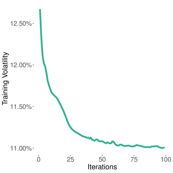
(a) Training volatility.

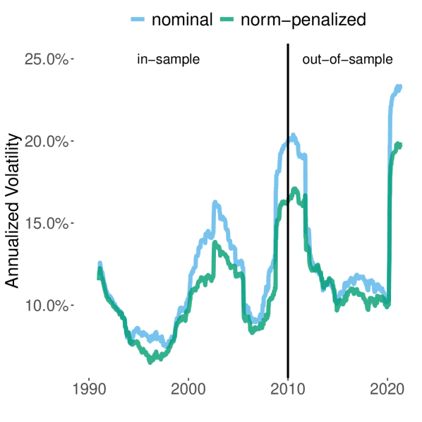
(b) Rolling $3$-year volatility.

Figure 2: In-sample training volatility and rolling $3$-year annualized volatility of the nominal and norm-penalized minimum-variance portfolios.

3 Experiments

We present two experiments: a minimum-variance portfolio optimization on US stocks data and a maximum Sharpe ratio optimization on global commodity futures data. The US stocks data consists of $255$ liquid US stocks traded on major U.S. exchanges (NYSE, NASDAQ, AMEX, ARCA). Data is provided by Quandl and is summarized in Table 3 in Appendix B. Weekly price data is given from January $1990$ through May $2021$. The futures markets are summarized in Table 4. Futures data is given from March $1986$ through May $2021$, and is provided by Commodity Systems Inc. The returns of futures contracts are computed directly from the price data and are in excess of the risk-free rate.

We consider several norm-penalty models, summarized below.

1. Nominal: the nominal MVO program: $P(\operatorname{\bf z})=0.$

2. L2: user-defined $L_{2}$-norm penalty: $P(\operatorname{\bf z})=\frac{\operatorname{\bm{\gamma}}_{2}}{2}\lVert\operatorname{\bf z}\rVert_{2}^{2}.$

3. L2-COV: user-defined following Goldfarb and Iyengar (2003) and letting $\operatorname{\bf D}=\hat{\operatorname{\bf W}}^{\frac{1}{2}}\hat{\operatorname{\bm{\beta}}}$, where $\hat{\operatorname{\bf W}}$ denotes the covariance matrix of feature variables: $P(\operatorname{\bf z})=\frac{\operatorname{\bm{\gamma}}_{2}}{2}\lVert\operatorname{\bf D}\operatorname{\bf z}\rVert_{2}^{2}.$

4. L1: user-defined $L_{1}$-norm penalty: $P(\operatorname{\bf z})=\operatorname{\bm{\gamma}}_{1}\lVert\operatorname{\bf z}\rVert_{1}.$

5. EN: user-defined elastic-net penalty with mixing coefficient $\alpha=0.5$ and ${P(\operatorname{\bf z})=\alpha\operatorname{\bm{\gamma}}_{1}\lVert\operatorname{\bf z}\rVert_{1}+(1-\alpha)\frac{\operatorname{\bm{\gamma}}_{2}}{2}\lVert\operatorname{\bf z}\rVert_{2}^{2}}.$

6. L2-P: parameterized $L_{2}$-norm penalty with $\operatorname{\bf D}(\operatorname{\bm{\theta}}_{2})=\operatorname{diag}(\operatorname{\bm{\theta}}_{2})$, $\operatorname{\bm{\theta}}_{2}\in\mathbb{R}_{+}^{d_{z}}$ and ${P(\operatorname{\bf z})=\frac{\operatorname{\bm{\gamma}}_{2}}{2}\lVert\operatorname{\bf D}(\operatorname{\bm{\theta}}_{2})\operatorname{\bf z}\rVert_{2}^{2}}.$

7. L2-COV-P: parameterized $L_{2}$-norm penalty with $\operatorname{\bf D}(\operatorname{\bm{\theta}}_{2})=\hat{\operatorname{\bf W}}^{\frac{1}{2}}\operatorname{\bm{\theta}}_{2}$ and ${P(\operatorname{\bf z})=\frac{\operatorname{\bm{\gamma}}_{2}}{2}\lVert\operatorname{\bf D}(\operatorname{\bm{\theta}}_{2})\operatorname{\bf z}\rVert_{2}^{2}}.$

8. L1-P: parameterized $L_{1}$-norm penalty with $\operatorname{\bf E}(\operatorname{\bm{\theta}}_{1})=\operatorname{diag}(\operatorname{\bm{\theta}}_{1})$, $\operatorname{\bm{\theta}}_{1}\in\mathbb{R}_{+}^{d_{z}}$ and ${P(\operatorname{\bf z})=\operatorname{\bm{\gamma}}_{1}\lVert\operatorname{\bf E}(\operatorname{\bm{\theta}}_{1})\operatorname{\bf z}\rVert_{1}}.$

9. EN-P: parameterized elastic-net penalty with mixing coefficient $\alpha=0.5$, ${\operatorname{\bf D}(\operatorname{\bm{\theta}}_{2})=\operatorname{diag}(\operatorname{\bm{\theta}}_{2})}$, $\operatorname{\bf E}(\operatorname{\bm{\theta}}_{1})=\operatorname{diag}(\operatorname{\bm{\theta}}_{1})$ and ${P(\operatorname{\bf z})=\alpha\operatorname{\bm{\gamma}}_{1}\lVert\operatorname{\bf E}(\operatorname{\bm{\theta}}_{1})\operatorname{\bf z}\rVert_{1}+(1-\alpha)\frac{\operatorname{\bm{\gamma}}_{2}}{2}\lVert\operatorname{\bf D}(\operatorname{\bm{\theta}}_{2})\operatorname{\bf z}\rVert_{2}^{2}}.$

We refer the reader to Appendix A for full implementation details.

Note that the norm-penalty models, described above, can be divided into two groups:

1. User-defined: the norm-penalty is pre-defined by the user and the amount of regularization is optimized by solving Program $\eqref{eq:stoch_discrete}$.

2. Parameterized: the norm-penalty is parameterized and therefore the norm-penalty parameters and amount of regularization are jointly optimized by solving Program $\eqref{eq:stoch_discrete}$.

Both experiments consist of $30$ randomized trials where, at the beginning of each trial, a basket of $n$ assets is randomly drawn from the universe of available assets and held constant throughout the duration of the trial. Portfolios are formed at the close of each week and rebalanced on a weekly basis. All experiments use data from January $1990$ through December $2009$ for training. Performance is evaluated over the out-of-sample period from January $2010$ through May $2021$. Our analysis focuses on comparing the out-of-sample portfolio objectives, defined in Equation $\eqref{eq:costs}$, of the norm-penalized portfolios relative to the nominal MVO program.

In all experiments we estimate the penalty parameters using the end-to-end neural network framework, described in Section 2.4. Both the primal and dual norm-penalized QP layers are implemented by applying the ADMM layer, described in Sections 2.2 and 2.3. All portfolio optimizations under consideration are either unconstrained or contain linear equality constraints and box inequality constraints. Indeed, under these conditions, the ADMM layer implementation is preferred for its reported computational efficiency and ability to support larger scale portfolio optimization problems with $100-1000$ decision variables and thousands of training examples (Butler and Kwon, 2021a).

3.1 Experiment 1: US stocks data

We consider the long-only, fully invested minimum-variance optimization $(\mathbb{S}=\{\operatorname{\bf z}\mid\operatorname{\bf 1}^{T}\operatorname{\bf z}=1,\operatorname{\bf z}\geq 0\})$ on US stocks data, described in Table 3. The norm-penalty parameters are determined by solving Program $\eqref{eq:stoch_discrete}$ to minimize the variance decision cost, $c_{\text{MV}}$. Asset mean returns are estimated by least-squares according to Equation $\eqref{eq:y_hat}$. The feature variables, $\mathop{\mathrm{\operatorname{\bf x}}^{(i)}}\in\mathbb{R}^{5}$, are given by the Famma-French Five factor model with data provided by the Kenneth R. French data library. We estimate the time-varying covariance of feature variables, $\mathop{\mathrm{\hat{\operatorname{\bf W}}}^{(i)}}$, by applying a simple moving average covariance evaluated over the trailing $52$-weeks. The asset covariance matrix, $\mathop{\mathrm{\hat{\operatorname{\bf V}}}^{(i)}}$, is given by Equation $\eqref{eq:y_hat}$. In each trial experiment we randomly draw $n=50$ stocks from the asset universe.

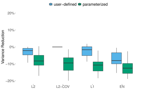
Figure 3: Out-of-sample percent variance cost reduction of norm-penalized minimum-variance portfolios relative to the nominal minimum-variance portfolio evaluated over $30$ randomized trials

Figure 3 reports the out-of-sample percent reduction in variance of the norm-penalized minimum-variance portfolios relative to the nominal minimum-variance portfolio. With the exception of the L2-COV model, all norm-penalized portfolios reduce the out-of-sample portfolio variance. We observe that the user-defined models produce a marginal $0\%-7\%$ average reduction in out-of-sample variance. In contrast, the parameterized models reduce the out-of-sample variance by $9\%-14\%$ on average. For both user-defined and parameterized models, the EN penalty, which contains both $L1$ and $L2$-norm penalties, produces the smallest average out-of-sample variance.

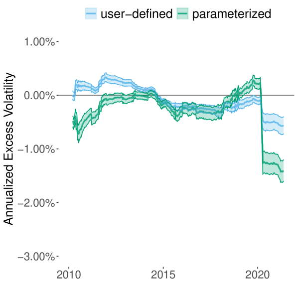
(a) L2.

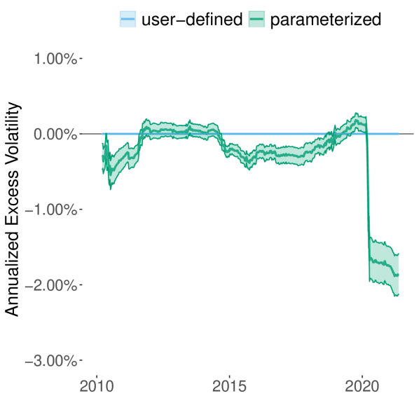
(b) L2-COV.

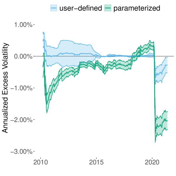
(c) L1.

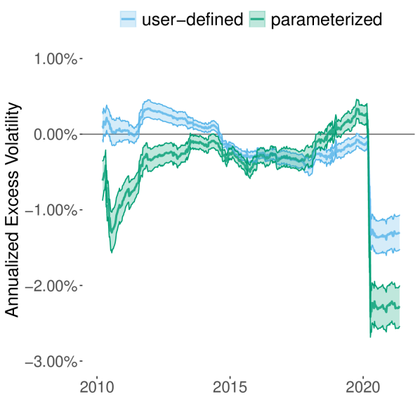
(d) EN.

Figure 4: Out-of-sample rolling average $3$-year excess annualized volatility with $95\%$ confidence interval evaluated over $30$ randomized trials.

Figure 4 reports the out-of-sample rolling average $3$-year annualized volatility difference between the norm-penalized minimum-variance portfolios and the nominal minimum-variance portfolio. The shaded regions denote the $95\%$ confidence interval evaluated over $30$ randomized trials. Note that values less than $0\%$ indicate that the norm-penalized portfolios produce a lower realized volatility over that time period. For user-defined models we generally observe insignificant difference in out-of-sample volatility with values oscillating around the zero line for the majority of the out-of-sample period. Notably, the L2-COV model results in a $0\%$ reduction in volatility, which is not surprising given that the penalty structure is closely related to the covariance estimate itself. In contrast, we observe that in normal market conditions, the parameterized models result in a consistent reduction in out-of-sample volatility, with the exception of $2018-2019$ where the norm-penalized models produce marginally higher volatility. Both the user-defined and parameterized models exhibit a large reduction in realized volatility during the COVID-19 crisis of $2020-2021$. During that time the user-defined models result in a $0\%-1.32\%$ average reduction in annualized volatility whereas the parameterized models result in a $1.27\%-2.27\%$ annualized volatility reduction in comparison to the nominal portfolio.

Finally in Table 1 we report the average out-of-sample economic performance for the nominal and norm-penalized minimum-variance portfolios. We also report standard errors evaluated over the $30$ randomized trials. Observe that, with the exception of the L2-COV model, all norm-penalized models produce a lower out-of-sample average volatility; which is encouraging as this is exactly the objective for which the norm-penalty parameters are optimized. With the exception of the L2 model, all norm-penalized models produce lower average returns. The resulting impact on Sharpe ratios is mixed with the L2 and L2-COV-P models producing marginally higher Sharpe ratios and all other models producing lower out-of-sample risk-adjusted returns.

	Mean	$\sigma_{\text{Mean}}$	Volatility	$\sigma_{\text{Vol}}$	Sharpe Ratio	$\sigma_{\text{Sharpe}}$
Nominal	0.1265	0.0020	0.1411	0.0016	0.8682	0.0138
L2	0.1267	0.0017	0.1387	0.0014	0.8852	0.0138
L2-P	0.1236	0.0019	0.1350	0.0014	0.8862	0.0141
L2-COV	0.1265	0.0020	0.1411	0.0016	0.8681	0.0138
L2-COV-P	0.1246	0.0021	0.1334	0.0013	0.9039	0.0163
L1	0.1151	0.0026	0.1403	0.0018	0.7906	0.0138
L1-P	0.1048	0.0020	0.1320	0.0011	0.7626	0.0143
EN	0.1163	0.0016	0.1357	0.0012	0.8271	0.0123
EN-P	0.1081	0.0020	0.1313	0.0012	0.7923	0.0150

Table 1: Average and standard errors of out-of-sample economic performance for the nominal and norm-penalized minimum-variance portfolios evaluated over $30$ randomized trials.

3.2 Experiment 2: global futures data

We consider an unconstrained mean-variance optimization $(\mathbb{S}=\mathbb{R}^{d_{z}})$ on global futures data, described in Table 4. The norm-penalty parameters are determined by solving Program $\eqref{eq:stoch_discrete}$ to minimize the Sharpe ratio decision cost, $c_{\text{SR}}$. Asset mean returns are estimated by least-squares according to Equation $\eqref{eq:y_hat}$. The feature variables, $\mathop{\mathrm{\operatorname{\bf x}}^{(i)}}\in\mathbb{R}^{5}$, are the average trailing $1$-month risk-adjusted return for each market, averaged by asset class. The asset covariance matrix, $\mathop{\mathrm{\hat{\operatorname{\bf V}}}^{(i)}}$, is estimated by a simple moving average covariance evaluated over the trailing $52$ weeks and the risk-aversion parameter is set to $\delta=20$. In each trial we randomly draw $n=20$ assets from the asset universe.

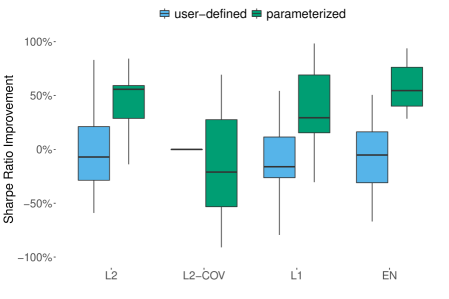
Figure 5: Out-of-sample Percent Sharpe ratio improvement of norm-penalized mean-variance portfolios evaluated over $30$ randomized trials

Figure 5 reports the out-of-sample percent improvement in Sharpe ratios of the norm-penalized MVO portfolios relative to the nominal MVO portfolio. Note here that values greater than $0\%$ indicate an increase in Sharpe ratio, which we seek to maximize. With the exception of the L2-COV-P model, all other norm-penalized portfolios increase the average out-of-sample Sharpe ratio with median percent improvements ranging from $0\%-45.7\%$. We note that the improvement in the out-of-sample portfolio objective is not as consistent as the reduction in variance exhibited by the stocks data experiment, with many trials resulting in lower out-of-sample Sharpe ratios. As before we note that the parameterized models result in a larger improvement in out-of-sample portfolio objectives in comparison to their user-defined counterparts. The parameterized models produce median out-of-sample Sharpe ratio improvements ranging from $-8.1\%-45.7\%$ whereas the user-defined models produce median out-of-sample Sharpe ratio improvements ranging from $0\%-8.5\%$. Lastly, parameterized models exhibit a larger variance in out-of-sample Sharpe ratio, suggesting that the models may be overfitting the in-sample data.

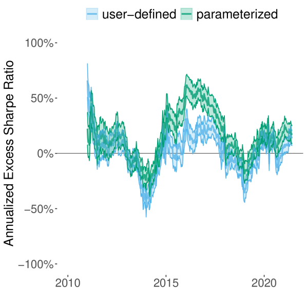
(a) L2.

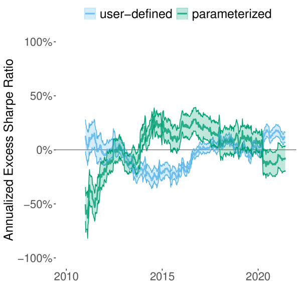
(b) L2-COV.

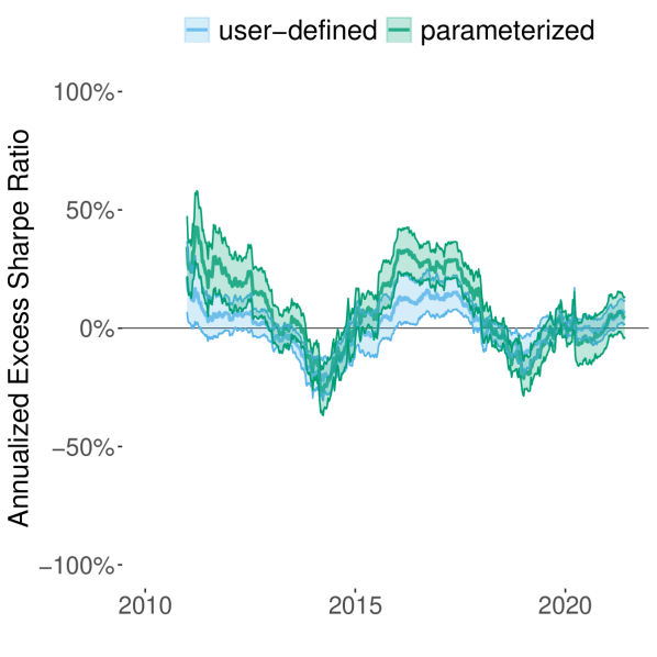
(c) L1.

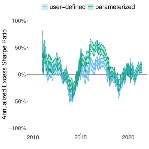
(d) EN.

Figure 6: Out-of-sample rolling average $3$-year excess annualized Sharpe ratio with $95\%$ confidence interval evaluated over $30$ randomized trials. .

Figure 6 reports the out-of-sample rolling average $3$-year annualized Sharpe ratio difference and $95\%$ confidence interval between the norm-penalized MVO portfolios and the nominal MVO portfolio. Note that values greater than $0\%$ indicate that the norm-penalized portfolios produce a higher realized Sharpe ratio over that time period. As expected, the parameterized models produce higher and more consistent improvements in Sharpe ratio in comparison to the corresponding user-defined models. The difference, however, is not statistically significant and displays considerable overlap in confidence intervals. Moreover, during both $2013-2014$ and $2018-2019$ we observe that the parameterized norm-penalized MVO portfolios produce lower out-of-sample Sharpe ratios in comparison to the nominal MVO.

Lastly in Table 2 we report the average out-of-sample economic performance and corresponding standard errors for the nominal and norm-penalized MVO portfolios. As expected, the norm-penalized portfolios exhibit a reduction in portfolio volatility. With the exception of the L2-COV-P model, the reduction in volatility exceeds the corresponding reduction in mean return, thus producing higher average out-of-sample Sharpe ratios. The average Sharpe ratio improvement ranges from $4.8\%-48.3\%$. Again these results are encouraging as the norm-penalty parameters are directly optimized to maximize the Sharpe ratio. In general we find that the L2-P and EN-P models produce significant average Sharpe ratio improvements, with average values of $0.4326-0.4658$ in comparison to the nominal Sharpe ratio of $0.3184$.

	Mean	$\sigma_{\text{Mean}}$	Volatility	$\sigma_{\text{Vol}}$	Sharpe Ratio	$\sigma_{\text{Sharpe}}$
Nominal	0.2118	0.0236	0.6393	0.0382	0.3184	0.0314
L2	0.0581	0.0047	0.1652	0.0065	0.3519	0.0227
L2-P	0.0945	0.0061	0.2028	0.0056	0.4658	0.0267
L2-COV	0.1092	0.0120	0.3385	0.0255	0.3296	0.0315
L2-COV-P	0.1090	0.0155	0.3469	0.0117	0.3108	0.0419
L1	0.1733	0.0212	0.4954	0.0436	0.3425	0.0273
L1-P	0.1627	0.0190	0.4243	0.0357	0.3757	0.0346
EN	0.0584	0.0048	0.1655	0.0067	0.3530	0.0227
EN-P	0.0857	0.0064	0.1983	0.0068	0.4326	0.0289

Table 2: Average and standard errors of out-of-sample economic performance for the nominal and norm-penalized MVO portfolios evaluated over $30$ randomized trials.

4 Conclusion and future work

In this paper we augmented the nominal mean-variance program with a convex combination of parameterized $L_{1}$ and $L_{2}$-norm penalty functions. A traditional approach would pre-specify the penalty structure and then optimize for the amount of regularization. Alternatively, we presented a data-driven framework for optimizing the parameterized penalty structures such that the resulting penalized program induces optimal portfolio decision-making. The parameter estimation problem is cast as a bi-level program and optimized by first-order gradient descent. Specifically, we structured the learning process an an end-to-end neural network with differentiable quadratic programming layers. We proposed a novel technique for differentiating the optimal solution, $\operatorname{\bf z}^{*}$, with respect to the parameterized $L_{1}$-norm, which solves the dual program - a box-constrained QP - and then recovers the primal solution from the optimal dual variables.

We presented several experiments using both US stocks and global futures data and demonstrated the benefit of the data-driven approach. In general we find that the parameterized norm-penalty models, in which the exact penalty structure is learned from the data, provide improved out-of-sample portfolio objectives in comparison to the nominal and user-defined norm-penalized portfolios. Our experiments should be interpreted as a proof-of-concept and we acknowledge that further testing with alternative datasets, and under varying prediction model and portfolio constraint assumptions is required in order to better determine the efficacy of the data-driven solution. In particular, we note that the parameterized models, if poorly specified, risk overfitting the training dataset. We believe that a stochastic optimization framework whereby model parameters are optimized in order to minimize a cross-validation cost may attenuate the propensity for model overfit and is an active area of research.

Appendix A Implementation details

The norm-penalty coefficients, $\operatorname{\bm{\gamma}}_{1}$ and $\operatorname{\bm{\gamma}}_{2}$ are constrained to the positive real orthant which is satisfied by applying following exponential transformation:

$$\operatorname{\bm{\gamma}}_{1}\leftarrow e^{\operatorname{\bm{\gamma}}_{1}}\qquad\text{and}\operatorname{\bm{\gamma}}_{2}\leftarrow e^{\operatorname{\bm{\gamma}}_{1}}.$$

Coefficients are initialized at $\operatorname{\bm{\gamma}}_{1}=-4$ and $\operatorname{\bm{\gamma}}_{2}=-4$. The diagonal matrices ${\operatorname{\bf E}(\operatorname{\bm{\theta}}_{1})=\operatorname{diag}(\operatorname{\bm{\theta}}_{1})}$ and ${\operatorname{\bf D}(\operatorname{\bm{\theta}}_{2})=\operatorname{diag}(\operatorname{\bm{\theta}}_{2})}$ are constrained to be positive semidefinite, which we implement by applying a relu transformation:

$$\operatorname{\bm{\theta}}_{1}\leftarrow\max(\operatorname{\bm{\theta}}_{1},0)\quad\text{and}\quad\operatorname{\bm{\theta}}_{2}\leftarrow\max(\operatorname{\bm{\theta}}_{2},0)$$

The parameters are initialized randomly from the standard uniform distributions:

$$\operatorname{\bm{\theta}}_{1}\in[0,1]^{d_{z}},\quad\operatorname{\bm{\theta}}_{2}\in[0,1]^{d_{z}}$$

All parameters are optimized by applying the ADAM gradient descent routine [Kingma and Ba, 2014]. We find that using $100\%$ of the training observations with a learning rate of $0.10$ results in numerically stable and consistent parameter estimation. All experiments were conducted on an Apple Mac Pro computer ($2.7$ GHz $12$-Core Intel Xeon E5,$128$ GB $1066$ MHz DDR3 RAM) running macOS ‘Catalina’. The software was written using the R programming language (version $4.0.0$) and torch (version $0.6.0$).

The code snippet, presented below demonstrates how to implement the optimization of the norm-penalty parameters as an end-to-end trainable neural network for the example provided in Section 2.4 . We refer to the open-source R package lqp (learning quadratic programs), available here: https://github.com/butl3ra/lqp, for more details. Note that the norm-penalty contains a parameterized $L_{1}$-norm and therefore we implement the dual solver with fixed-point implicit differentiation, as described in Section 2.3.

# — setup solver control: control = nn_qp_control(solver = ’con_l1’, backprop = ’fixed_point’) # — p_model: p_model = nn_constant(value = torch_zeros(c(1,n_y,1))) # — Q_model: Q_model = nn_constant(value = Q_is_t) # — A_model and b_model: A_model = nn_constant(value = torch_ones(c(1,1,n_y))) b_model = nn_constant(value = torch_ones(c(1))) # — G_model and h_model: G_model = nn_constant(value = -torch_eye(n_y)$unsqueeze(1))h_{m}odel=nn_{c}onstant(value=torch_{z}eros(c(1,n_{y},1)))#---E_{m}odelandlambda_{1}:E=nn_{p}arameter(as_{t}orch_{t}ensor(diag(runif(n_{y})),requires_{g}rad=TRUE))E_{m}odel=nn_{s}equential(nn_{c}onstant(value=E),nn_{u}nsqueeze(dim=1),nn_{r}elu())lambda_{1}=nn_{p}arameter(as_{t}orch_{t}ensor(-4,requires_{g}rad=TRUE))lambda_{1}{}_{m}odel=nn_{s}equential(nn_{c}onstant(value=lambda_{1}),nn_{e}xp())#---D_{m}odelandlambda_{2}:D_{m}odel=nn_{q}uad_{f}orm_{c}onst(in_{f}eatures=n_{x},out_{f}eatures=n_{y},x_{m}at=Q_{x})lambda_{2}=nn_{p}arameter(as_{t}orch_{t}ensor(-4,requires_{g}rad=TRUE))lambda_{2}{}_{m}odel=nn_{s}equential(nn_{c}onstant(value=lambda_{2}),nn_{e}xp())\par#---norm-penalizedqpmodel:model=nn_{l}qp(Q_{m}odel=Q_{m}odel,p_{m}odel=p_{m}odel,A_{m}odel=A_{m}odel,b_{m}odel=b_{m}odel,G_{m}odel=G_{m}odel,h_{m}odel=h_{m}odel,D_{m}odel=D_{m}odel,lambda_{2}{}_{m}odel=lambda_{2}{}_{m}odel,E_{m}odel=E_{m}odel,lambda_{1}{}_{m}odel=lambda_{1}{}_{m}odel,control=control)optimizer<-optim_{a}dam(model$parameters, lr = 0.10) #—————- training loop ——————- for (t in 1:100 ) # — forward pass z = model(x = x_is_t) z = torch_sum_1(z,dim = 2) # — compute loss loss ¡- nnf_var_loss(z = z, y_is_t$unsqueeze(3))#---backpropagation:optimizer$zero_grad() loss$backward()#---updateparams:optimizer$step()

Appendix B Data summary

GICS Sector				Stock Symbols
Communication	CBB	CMCSA	DIS	FOX	IPG	LUMN	MDP	NYT
	T	VOD	VZ
Consumer	BBY	CBRL	CCL	F	GPC	GPS	GT	HAS
Discretionary	HD	HOG	HRB	JWN	LB	LEG	LEN	LOW
	MCD	NKE	NVR	NWL	PHM	PVH	ROST	TGT
	TJX	VFC	WHR	WWW
Consumer	ADM	ALCO	CAG	CASY	CHD	CL	CLX	COST
Staples	CPB	FLO	GIS	HSY	K	KMB	KO	KR
	MO	PEP	PG	SYY	TAP	TR	TSN	UVV
	WBA	WMK	WMT
Energy	AE	APA	BKR	BP	COP	CVX	EOG	HAL
	HES	MRO	OKE	OXY	SLB	VLO	WMB	XOM
Financials	AFG	AFL	AIG	AJG	AON	AXP	BAC	BEN
	BK	BXS	C	GL	JPM	L	LNC	MMC
	PGR	PNC	RJF	SCHW	STT	TROW	TRV	UNM
	USB	WFC	WRB	WTM
Health Care	ABMD	ABT	AMGN	BAX	BDX	BIO	BMY	CAH
	CI	COO	CVS	DHR	HUM	JNJ	LLY	MDT
	MRK	OMI	PFE	PKI	SYK	TFX	TMO	VTRS
	WST
Industrials	ABM	AIR	ALK	AME	AOS	BA	CAT	CMI
	CSL	CSX	DE	DOV	EFX	EMR	ETN	FDX
	GD	GE	GWW	HON	IEX	ITW	JCI	KSU
	LMT	LUV	MAS	MMM	NOC	NPK	NSC	PCA
	RPH	PNR	ROK	ROL	RTX	SNA	SWK	TXT
	UNP
Information	AAPL	ADBE	ADI	ADP	ADSK	AMAT	AMD	GLW
Technology	HPQ	IBM	INTC	MSFT	MSI	MU	ORCL	ROG
	SWKS	TER	TXN	TYL	WDC	XRX
Materials	APD	AVY	BLL	CCK	CRS	ECL	FMC	GLT
	IFF	IP	MOS	NEM	NUE	OLN	PPG	SEE
	SHW	SON	VMC
Real Estate	ALX	FRT	GTY	HST	PEAK	PSA	VNO	WRI
	WY
Utilities	AEP	ATO	BKH	CMS	CNP	D	DTE	DUK
	ED	EIX	ETR	EVRG	EXC	LNT	NEE	NFG
	NI	NJR	OGE	PEG	PNM	PNW	PPL	SJW
	SO	SWX	UGI	WEC	XEL

Table 3: U.S. stock data, sorted by GICS Sector. Data provided by Quandl.

Asset Class			Market (Symbol)
Energy		WTI crude (CL)	Heating oil (HO)	Gasoil (QS)
		RBOB gasoline (XB)
Grain		Bean oil (BO)	Corn (C)	KC Wheat (KW)
		Soybean (S)	Soy meal (SM)	Wheat (W)
Livestock		Feeder cattle (FC)	Live cattle (LC)	Lean hogs (LH)
Metal		Gold (GC)	Copper (HG)	Palladium (PA)
		Platinum (PL)	Silver (SI)
Soft		Cocoa (CC)	Cotton (CT)	Robusta Coffee (DF)
		Coffee (KC)	Canola (RS)	Sugar (SB)

Table 4: Futures market data, following Bloomberg symbology. Data provided by Commodity Systems Inc.

References

- Agrawal et al. [2019] Akshay Agrawal, Brandon Amos, Shane Barratt, Stephen Boyd, Steven Diamond, and J. Zico Kolter. Differentiable convex optimization layers. In Advances in Neural Information Processing Systems, volume 32, pages 9562–9574. Curran Associates, Inc., 2019.
- Amos and Kolter [2017] Brandon Amos and J. Zico Kolter. Optnet: Differentiable optimization as a layer in neural networks, 2017. URL https://arxiv.org/abs/1703.00443.
- Amos et al. [2019] Brandon Amos, Ivan Dario Jimenez Rodriguez, Jacob Sacks, Byron Boots, and J. Zico Kolter. Differentiable mpc for end-to-end planning and control, 2019. URL http://arxiv.org/abs/1810.13400.
- Ben-Tal et al. [2009] A Ben-Tal, L El Ghaoui, and ANemirovski. Robust Optimization. Princeton University Press, 2009.
- Ben-Tal and Nemirovski [2000] Aharon Ben-Tal and Arkadi Nemirovski. Robust solutions of linear programming problems contaminated with uncertain data. Mathematical Programming, 88:411–424, 01 2000. doi: 10.1007/PL00011380.
- Bertsimas and Kallus [2020] Dimitris Bertsimas and Nathan Kallus. From predictive to prescriptive analytics. Management Science, 66(3):1025–1044, 2020.
- Bertsimas and Sim [2004] Dimitris Bertsimas and Melvyn Sim. The price of robustness. Operations Research, 52:35–53, 02 2004. doi: 10.1287/opre.1030.0065.
- Bertsimas et al. [2014] Dimitris Bertsimas, Vishal Gupta, and Nathan Kallus. Data-driven robust optimization, 2014.
- Black and Litterman [1991] F. Black and R. Litterman. Asset allocation combining investor views with market equilibrium. Journal of Fixed Income, 1(2):7–18, 1991.
- Boyd and Vandenberghe [2004] Stephen Boyd and Lieven Vandenberghe. Convex Optimization. Cambridge University Press, 2004. doi: 10.1017/CBO9780511804441.
- Butler and Kwon [2021a] Andrew Butler and Roy Kwon. Efficient differentiable quadratic programming layers: an admm approach, 2021a. URL https://arxiv.org/abs/2112.07464.
- Butler and Kwon [2021b] Andrew Butler and Roy Kwon. Covariance estimation for risk-based portfolio optimization: an integrated approach. Journal of Risk, 24(2), December 2021b.
- Butler and Kwon [2021c] Andrew Butler and Roy H. Kwon. Integrating prediction in mean-variance portfolio optimization, 2021c. URL https://arxiv.org/abs/2102.09287.
- Chevalier et al. [2022] Guillaume Chevalier, Guillaume Coqueret, and Thomas Raffinot. Supervised portfolios. SSRN Electronic Journal, 4 2022. URL https://ssrn.com/abstract=3954109.
- Chopra and Ziemba [1993] Vijay Kumar. Chopra and William T. Ziemba. The effect of errors in means, variances, and covariances on optimal portfolio choice. The Journal of Portfolio Management, 19(2):6–11, 1993. ISSN 0095-4918. doi: 10.3905/jpm.1993.409440. URL https://jpm.pm-research.com/content/19/2/6.
- DeMiguel et al. [2009] Victor DeMiguel, Lorenzo Garlappi, Raman Uppal, and L Nogales. A generalized approach to portfolio optimization: improving performance by constraining portfolio norms. Management Science, 55(5):798–812, 2009.
- Donti et al. [2017] Priya Donti, Brandon Amos, and J. Zico Kolter. Task-based end-to-end model learning in stochastic optimization. In I. Guyon, U. V. Luxburg, S. Bengio, H. Wallach, R. Fergus, S. Vishwanathan, and R. Garnett, editors, Advances in Neural Information Processing Systems, volume 30, pages 5484 – 5494. Curran Associates, Inc., 2017.
- Drees and Starica [2002] Holger Drees and Catalin Starica. A simple non-stationary model for stock returns, 2002.
- Elmachtoub and Grigas [2017] Adam Elmachtoub and Paul Grigas. Smart ‘predict, then optimize’. Management Science, 10 2017. doi: 10.1287/mnsc.2020.3922.
- Elmachtoub et al. [2020] Adam N. Elmachtoub, Jason Cheuk Nam Liang, and Ryan McNellis. Decision trees for decision-making under the predict-then-optimize framework, 2020. URL http://arxiv.org/abs/2003.00360.
- Engle [1982] Robert F. Engle. Autoregressive conditional heteroskedasticity with estimates of the variance of uk inflation. Econometrica, 50(1):987–1008, 1982.
- Feng and Simon [2017] Jean Feng and Noah Simon. Gradient-based regularization parameter selection for problems with non-smooth penalty functions, 2017.
- Goldfarb and Iyengar [2003] D. Goldfarb and G. Iyengar. Robust portfolio selection problems. Mathematics of Operations Research, 28(1):1–38, 2003.
- Grigas et al. [2021] Paul Grigas, Meng Qi, Zuo-Jun, and Shen. Integrated conditional estimation-optimization, 2021. URL http://arxiv.org/abs/2110.12351.
- Hastie et al. [2001] Trevor Hastie, Robert Tibshirani, and Jerome Friedman. The Elements of Statistical Learning. Springer Series in Statistics. Springer New York Inc., New York, NY, USA, 2001.
- Ho et al. [2015] Michael Ho, Zheng Sun, and Jack Xin. Weighted elastic net penalized mean-variance portfolio design and computation. SIAM Journal on Financial Mathematics, 6(1):1220–1244, 2015.
- Ichnowski et al. [2021] Jeffrey Ichnowski, Paras Jain, Bartolomeo Stellato, Goran Banjac, Michael Luo, Francesco Borrelli, Joseph E. Gonzalez, Ion Stoica, and Ken Goldberg. Accelerating quadratic optimization with reinforcement learning, 2021. URL https://arxiv.org/abs/2107.10847.
- Jobson and Korkie [1980] J.D. Jobson and Bob Korkie. Estimation for markowitz efficient portfolios. Journal of the American Statistical Association, pages 544 – 555, 1980.
- Jobson and Korkie [1982] J.D. Jobson and Bob Korkie. Potential performance and tests of portfolio efficiency. Journal of Financial Economics, 10(4):433 – 466, 1982.
- Kim et al. [2008] Seung-Jean Kim, K. Koh, M. Lustig, Stephen Boyd, and Dimitry Gorinevsky. An interior-point method for large-scale l1-regularized least squares. Selected Topics in Signal Processing, IEEE Journal of, 1:606 – 617, 01 2008. doi: 10.1109/JSTSP.2007.910971.
- Kingma and Ba [2014] Diederik P. Kingma and Jimmy Ba. Adam: A method for stochastic optimization, 2014. URL https://arxiv.org/abs/1412.6980.
- Ledoit and Wolf [2004a] Olivier Ledoit and Michael Wolf. Honey, i shrunk the sample covariance matrix. The Journal of Portfolio Management, 30(4):110–119, 2004a.
- Ledoit and Wolf [2004b] Olivier Ledoit and Michael Wolf. A well-conditioned estimator for large-dimensional covariance matrices. Journal of Multivariate Analysis, 88(2):365–411, 2004b.
- Ledoit and Wolf [2012] Olivier Ledoit and Michael Wolf. Nonlinear shrinkage estimation of large-dimensional covariance matrices. The Annals of Statistics, 40(2):1024–1060, 2012.
- Lorraine and Duvenaud [2018] Jonathan Lorraine and David Duvenaud. Stochastic hyperparameter optimization through hypernetworks, 2018.
- Mandi and Guns [2020] Jayanta Mandi and Tias Guns. Interior point solving for lp-based prediction+optimisation, 2020. URL http://arxiv.org/abs/2010.13943.
- Mandi et al. [2019] Jaynta Mandi, Emir Demirovic, Peter. J Stuckey, and Tias Guns. Smart predict-and-optimize for hard combinatorial optimization problems, 2019. URL http://arxiv.org/abs/1911.10092.
- Markowitz [1952] H. Markowitz. Portfolio selection. Journal of Finance, 7(1):77–91, 1952.
- Michaud and Michaud [2008a] Richard Michaud and Robert Michaud. Efficient asset management: A practical guide to stock portfolio optimization and asset allocation. New York: Oxford University Press, 1, 2008a.
- Michaud and Michaud [2008b] Richard Michaud and Robert Michaud. Estimation error and portfolio optimization: A resampling solution. Journal of Investment Management, 6(1):8–28, 2008b.
- Pedregosa [2016] Fabian Pedregosa. Hyperparameter optimization with approximate gradient, 2016.
- Rumelhart et al. [1986] David E. Rumelhart, Geoffrey E. Hinton, and Ronald J. Williams. Learning representations by back-propagating errors. Nature, 323:533–536, 1986.
- Starica and Granger [2005] Catalin Starica and Clive Granger. Nonstationarities in stock returns. The Review of Economics and Statistics, 87(3):503–522, 2005.
- Stein [1956] Charles Stein. Inadmissibility of the usual estimator for the mean of a multivariate normal distribution. In Proceedings of the Third Berkeley Symposium on Mathematical Statistics and Probability, Volume 1: Contributions to the Theory of Statistics, pages 197–206, Berkeley, Calif., 1956. University of California Press. URL https://projecteuclid.org/euclid.bsmsp/1200501656.
- Tibshirani [1996] Robert Tibshirani. Regression shrinkage and selection via the lasso. Journal of the Royal Statistical Society, 58(1), 1996.
- Tikhonov [1963] A. N. Tikhonov. Solution of incorrectly formulated problemsand the regularization method. Soviet Mathematics, pages 1035–1038, 1963.
- Tutuncu and Koenig [2004] R. Tutuncu and M. Koenig. Robust asset allocation. Annals of Operations Research, 132:157–187, 2004.
- Uysal et al. [2021] Ayse Sinem Uysal, Xiaoyue Li, and John M. Mulvey. End-to-end risk budgeting portfolio optimization with neural networks, 2021. URL http://arxiv.org/abs/2107.04636.
- Yin et al. [2019] Chenyang Yin, Romain Perchet, and Francois Soupe. A practical guide to robust portfolio optimization. SSRN Electronic Journal, 1 2019. doi: 10.2139/ssrn.3490680.
- Zhu et al. [2009] Lei Zhu, Thomas Coleman, and Yuying li. Min-max robust and cvar robust mean-variance portfolios. Journal of Risk, 11, 03 2009. doi: 10.21314/JOR.2009.191.
- Zou and Hastie [2005] Hui Zou and Trevor Hastie. Regularization and variable selection via the elastic net. Journal of the Royal Statistical Society. Series B (Statistical Methodology), 67(2):301–320, 2005.