Non-uniqueness of weak solutions to 3D magnetohydrodynamic equations

Abstract.

We prove the non-uniqueness of weak solutions to 3D magnetohydrodynamic (MHD for short) equations. The constructed weak solutions do not conserve the magnetic helicity and can be close to any given smooth, divergence-free and mean-free velocity and magnetic fields. Furthermore, we prove that the weak solutions constructed by Beekie-Buckmaster-Vicol [2] for the ideal MHD can be obtained as a strong vanishing viscosity and resistivity limit of a sequence of weak solutions to MHD equations. This shows that, in contrast to the weak ideal limits, Taylor’s conjecture does not hold along the vanishing viscosity and resistivity limits. Unlike in the context of the NSE [13] and the ideal MHD [2], new types of velocity and magnetic flows, featuring both the refined spatial and temporal intermittency, are constructed to respect the geometry of MHD and to control the strong viscosity and resistivity. Compatible algebraic structure is derived in the convex integration scheme. More interestingly, the new intermittent flows indeed enable us to prove the aforementioned results for the hyper-viscous and hyper-resistive MHD equations up to the sharp exponent $5/4$, which coincides exactly with the Lions exponent for 3D hyper-viscous NSE.

1. Introduction and main results

1.1. Introduction

The problem of non-uniqueness of weak solutions to hydrodynamic models attract a lot of attention in the last decade. Significant progresses have been made towards the Euler equations and Navier-Stokes equations based on the convex integration method, which originates from the work by Nash [59] concerning the construction of $C^{1}$ isometric immersions of $S^{n}$ into ${\mathbb{R}}^{m}$ $(m\geq n+2)$ and was introduced by De Lellis-Székelyhidi in the pioneering paper [27] to 3D Euler equations.

Among various hydrodynamic models, the viscous and resistive MHD system is a canonical macroscopic model to describe the motion of conductive fluid, such as plasma or liquid metals, under a complicated interaction between the electromagnetic phenomenon and fluid dynamical phenomenon (see [50]). We refer the reader to [4, 5, 26, 61] for more physical interpretations of the MHD system.

The applicability of convex integration scheme to MHD equations is at an early stage (see [15] and the literature review below), and it is the objective of the present article. As a matter of fact, because of the strong coupling of the velocity and magnetic fields, the convex integration method requires the construction of both the velocity and magnetic fields in an appropriate way, in order to respect the geometry of MHD. This particular structural requirement, however, limits the oscillation directions and thus the spatial intermittency of flows, which results in a substantial difficulty to control the strong viscosity and resistivity.

More precisely, we are concerned with the three-dimensional MHD system on the torus ${\mathbb{T}}^{3}:=[-\pi,\pi]^{3}$,

$$\left\{\begin{aligned} &\partial_{t}u-\nu_{1}\Delta u+(u\cdot\nabla)u-(B\cdot\nabla)B+\nabla P=0,\\ &\partial_{t}B-\nu_{2}\Delta B+(u\cdot\nabla)B-(B\cdot\nabla)u=0,\\ &{\mathrm{div}}u=0,\quad{\mathrm{div}}B=0,\end{aligned}\right.$$ (1.1)

where $u=(u_{1},u_{2},u_{3})^{\top}(t,x)\in{\mathbb{R}}^{3}$, $B=(B_{1},B_{2},B_{3})^{\top}(t,x)\in{\mathbb{R}}^{3}$ and $P=P(t,x)\in{\mathbb{R}}$ correspond to the velocity field, magnetic field and pressure of the fluid, respectively, and $\nu_{1},\nu_{2}\geq 0$ are the viscous and resistive coefficients, respectively. We note that, in the case without magnetic fields, (1.1) reduces to the incompressible Navier-Stokes equation (NSE for short).

Another important model is the ideal MHD system, where the viscous and resistive coefficients vanish, namely,

$$\left\{\begin{aligned} &\partial_{t}u+(u\cdot\nabla)u-(B\cdot\nabla)B+\nabla P=0,\\ &\partial_{t}B+(u\cdot\nabla)B-(B\cdot\nabla)u=0,\\ &{\mathrm{div}}u=0,\quad{\mathrm{div}}B=0.\end{aligned}\right.$$ (1.2)

The incompressible ideal MHD system is the classical macroscopic model coupling the Maxwell equations to the evolution of an electrically conducting incompressible fluid (cf. [4, 26]). In the case $B\equiv 0$, (1.2) then reduces to the Euler equations.

The well-posedness problem of NSE and MHD has been extensively studied in the literature. For the initial data with finite energy, the existence of global weak solution $u$ to NSE was first proved by Leray [49] in 1934 and later by Hopf [41] in 1951 in bounded domains, which satisfies $u\in C_{weak}\big{(}[0,+\infty);L^{2}(\Omega)\big{)}\cap L^{2}\big{(}[0,+\infty);\dot{H}^{1}(\Omega)\big{)}$, $\Omega={\mathbb{R}}^{3}$ or $\mathbb{T}^{3}$, and obeys the following energy inequality

$$\|u(t)\|_{L^{2}}^{2}+2\nu\int_{t_{0}}^{t}\|{\nabla}u(s)\|_{L^{2}}^{2}{\rm d}s\leq\|u(t_{0})\|_{L^{2}}^{2}$$ (1.3)

for any $t>0$ and a.e. $t_{0}\geq 0$. The existence of Leray-Hopf solutions to generalized MHD equations was proved by Wu [67].

The uniqueness of Leray-Hopf solutions is considered as one of the most important issues in the mathematical fluid mechanics. The well known Ladyžhenskaya-Prodi-Serrin condition states that, the Leray-Hopf solution to NSE is regular and thus unique in the space $L^{\gamma}_{t}L^{p}_{x}$ for ${2}/{\gamma}+{3}/{p}\leq 1$ with $p>3$ (see [46, 60, 62]). The endpoint case $L^{\infty}_{t}L^{3}_{x}$ was solved by Escauriaza-Seregin-Šverák [33]. The well-posedness of NSE for small initial data in the space ${\rm BMO^{-1}}$ was proved by Koch-Tataru [48]. Moreover, Lions [52] obtained the well-posedness for the hyper-viscous NSE where the exponent of viscosity is bigger than $5/4$. Concerning the MHD type equations, the uniqueness of global classical solutions was proved by Wu [67], when the exponents of viscosity and resistivity are bigger than ${1}/{2}+{n}/{4}$, which is exactly the Lions exponent for the hyper-viscous NSE in dimension three $n=3$. Moreover, the uniqueness in the case analogous to the Ladyžhenskaya-Prodi-Serrin condition was proved by Zhou [69]. See also [51, 61, 63, 66, 68] and references therein.

Concerning the non-uniqueness problem of weak solutions, in the pioneering paper [27] De Lellis-Székelyhidi introduced the convex integration scheme to the 3D Euler equations and proved the existence of bounded solutions with compact support in space-time (see also [28]). Afterwards, significant progress towards the famous Onsager conjecture for the 3D Euler equations was made by De Lellis-Székelyhidi [29, 30]. The resolution of the Onsager conjecture was finally solved in $C_{x,t}^{\beta}\,(0<\beta<1/3)$ by Isett [42], and by Buckmaster-De Lellis-Székelyhidi-Vicol [11] for dissipative solutions. We also refer the reader to the papers [17, 21, 55] for Euler equations, [9, 19, 58, 57] for transport equations, and [12] for SQG equations. See also the surveys [31, 14, 15] on convex integration methods.

A recent break-through was obtained by Buckmaster-Vicol [13] for the 3D incompressible NSE. The non-uniqueness of weak solutions to NSE was proved in [13] by using an $L_{x}^{2}$-based intermittent convex integration scheme, which is efficient to handle the viscosity of NSE. Later, Luo-Titi [54] proved the non-uniqueness results for the 3D hyper-viscous NSE, whenever the exponent of viscosity is less than the Lions exponent $5/4$. Moreover, Luo-Qu [53] proved the non-uniqueness for the 2D hypoviscous NSE. The non-uniqueness results for the stationary NSE were proved by Cheskidov-Luo [18, 56]. We also refer to the works by Jia-Šverák [43, 44] for another method for the non-uniqueness issue of Leray-Hopf solutions in $L^{\infty}_{t}L^{3}_{x}$ under a certain assumption for the linearized Navier-Stokes operator, and Colombo-De Lellis-De Rosa [22] and De Rosa [32] for the non-uniqueness of Leray weak solutions to hypoviscous NSE with small viscosity.

Regarding the ideal MHD system (1.2), it posses a number of global invariants:

1. The total energy:  $\displaystyle\mathcal{E}(t)=\frac{1}{2}\int_{{\mathbb{T}}^{3}}|u(t,x)|^{2}+|B(t,x)|^{2}{\rm d}x$;

2. The cross helicity:   $\displaystyle\mathcal{H}_{\omega,B}(t)=\int_{{\mathbb{T}}^{3}}u(t,x)\cdot B(t,x){\rm d}x$;

3. The magnetic helicity:   $\displaystyle\mathcal{H}_{B,B}(t):=\int_{{\mathbb{T}}^{3}}A(t,x)\cdot B(t,x){\rm d}x$.

Here $A$ is a mean-free periodic vector field satisfying ${\mathrm{curl}}A=B$.

In analogy with the Onsager conjecture for Euler equations, it was conjectured in [15] that, $L^{3}_{t,x}$ (resp. $L^{3}_{t}B^{0}_{3,c_{0},x}$) is the critical space for the conservation of the magnetic helicity. More precisely, any weak solutions belonging to $L^{3}_{t,x}$ (resp. $L^{3}_{t}B^{0}_{3,c_{0},x}$) conserve the magnetic helicity (the rigidity part), while below the threshold there exist weak solutions violating the magnetic helicity conservation (the flexible part). Moreover, the space $C^{1/3}_{t,x}$ (resp. $L^{3}_{t}B^{1/3}_{3,{\infty},x}$) was conjectured to be the threshold for the conservation of the total energy and the cross helicity (see Remark 1.6 (ii) below).

These conjectures indeed lie in the general scope of the important issue to identify the critical/threshold regularity for the conservation laws. We refer to Klainerman [47] for the general formulations of different thresholds for supercritical Hamiltonian evolution equations, including the 3D MHD equations.

On the rigidity side, the magnetic helicity conservation for the 3D ideal MHD was proved in [45, 1, 34] and [16], respectively, for the critical spaces $L^{3}_{t,x}$ and $L^{3}_{t}B^{\alpha}_{3,{\infty},x}$ with ${\alpha}>0$. The corresponding rigidity results for the total energy conservation were proved in [16]. On the flexible side, weak solutions with non-trivial energy and vanishing magnetic helicity were first given in [8], by embedding the ideal MHD into the $2\frac{1}{2}$D Euler flow via a symmetry assumption. Wild solutions with compact support in space-time were first constructed by Faraco-Lindberg-Székelyhidi [36], via the $L^{\infty}_{t,x}$ convex integration scheme. The constructed solutions in [36] violate the energy conservation, while the magnetic helicity is still conserved and thus vanishes due to the compact support in time of solutions.

The delicate point, as observed by Beekie-Buckmaster-Vicol [2], is that the magnetic helicity is conserved under much milder regularity conditions. As a matter of fact, the magnetic helicity is commonly expected in the plasma physics to be conserved in the infinite conductivity limit, known as Taylor’s conjecture ([64, 65]). This conjecture was proved by Faraco and Lindberg [35] under the weak ideal limits, namely, the weak limits of Leray solutions to MHD (1.1).

For general weak solutions, Beekie-Buckmaster-Vicol [2] first constructed weak solutions in $C_{t}L^{2}_{x}$ violating the magnetic helicity conservation. Unlike in [36], the proof of [2] relies on the intermittent convex integration scheme, in which the intermittent shear flows are constructed to respect the geometry of MHD. The flexible part of the Onsager-type conjecture for the magnetic helicity was recently solved by Faraco-Lindberg-Székelyhidi [37], based on the convex integration via staircase laminates.

See also Dai [25] for the Hall MHD system where the Hall nonlinearity takes the dominant effect, and Feireisl-Li [38] for the ill-posedness of the MHD system where the fluid is compressible, inviscid and magnetically resistive.

As mentioned above, the strong coupling of the velocity and magnetic fields in MHD equations limits the intermittency of flows in the convex integration scheme. More precisely, for the NSE, the flows constructed in [13] have 3D spatial intermittency, which is essential to control the viscosity in NSE. Regarding the ideal MHD, the intermittent shear flows constructed in [2] have 1D intermittency which only permit to control the hypo-viscosity and hypo-resistivity $(-\Delta)^{\alpha}$ with $\alpha\in(0,1/2)$. Hence, both the above intermittent flows are not applicable to the viscous and resistive MHD (1.1) under consideration here.

The main purpose of this paper is to address the non-uniqueness problem of weak solutions for the canonical MHD system (1.1). By constructing a new class of intermittent velocity and magnetic flows adapted to the geometry of MHD, we are able to control the strong viscosity and resistivity. More interestingly, the new class of intermittent flows even enables us to achieve the non-uniqueness of weak solutions to a more general class of MHD type equations, for all the exponents of viscosity and resistivity less than the sharp Lions exponent, namely,

$$\left\{\begin{aligned} &\partial_{t}u+\nu_{1}(-\Delta)^{\alpha_{1}}u+(u\cdot\nabla)u-(B\cdot\nabla)B+\nabla P=0,\\ &\partial_{t}B+\nu_{2}(-\Delta)^{\alpha_{2}}B+(u\cdot\nabla)B-(B\cdot\nabla)u=0,\\ &{\mathrm{div}}u=0,\quad{\mathrm{div}}B=0,\end{aligned}\right.$$ (1.4)

where $\alpha_{1},\alpha_{2}\in(0,5/4)$, $\nu_{1},\nu_{2}\geq 0$. We note that, the value $5/4$ coincides with the Lions exponent for the well-posedness of the hyper-viscous NSE [52], and with the exponent $1/2+n/4$ for the well-posedness of generalized MHD in dimension three $n=3$ [67].

The constructed weak solutions can be close to any given divergence-free, mean-free velocity and magnetic fields. In particular, the weak solutions live in the space $L^{\gamma}_{t}W^{s,p}_{x}$ with $0\leq s<{2}/{p}+{1}/{\gamma}-3/2$, $1\leq p,\gamma<+{\infty}$, and do not conserve the magnetic helicity. Thus, this provides more examples in the spaces $L^{\gamma}_{t}W^{s,p}_{x}$ for the flexible part of the Onsager-type conjecture for the ideal MHD (1.2).

Another aim of the present work is to make some progress towards the understanding of the relationship between the non-uniqueness of solutions to the ideal MHD (1.2) and MHD equations (1.1) or (1.4), which in turn relates to the physical Taylor conjecture.

As pointed out in [2, 15], the weak solutions to the ideal MHD (1.2) with non-trivial magnetic helicity cannot be obtained as the weak ideal limits of MHD Leray-Hopf solutions. Instead, we prove that the weak solutions constructed by Beekie-Buckmaster-Vicol [2] can be obtained as a strong vanishing viscosity and resistivity limit of a sequence of weak solutions to the MHD equations (1.4), where the exponents ${\alpha}_{i}$ can be even larger than one. An interesting outcome is that, together with the non-conservative results in the work [2], this shows that Taylor’s conjecture does not hold along the vanishing viscosity and resistivity limits of general weak solutions, in contrast to the weak ideal limits of Leray weak solutions.

One of the main novelties of our proof is the construction of the velocity and magnetic flows with the refined spatial intermittency, which are designed specifically to have two oscillation directions and concentrate on small spatial cuboids. This structure enables us to gain an additional 1D spatial intermittency than that in the ideal MHD case [2], and thus to control the viscosity and resistivity $(-\Delta)^{{\alpha}_{i}}$ with ${\alpha}_{i}\in[0,1)$, $i=1,2$.

Another nice feature is that, the new intermittent flows have almost mutually disjoint supports. Actually, the intermittent flows have much smaller intersections, which provide almost 2D spatial intermittency and thus contribute negligible errors in the convex integration scheme. This in particular simplifies the control of the nonlinearities in MHD equations.

In order to pass beyond the border line ${\alpha}_{i}=1$, $i=1,2$, another key novelty of proof is the construction of the $L_{t}^{2}$-based temporal intermittent flows adapted to the structure of MHD. We introduce the high temporal oscillations in the velocity and magnetic flows. Rather than the pointwise analysis in time, we measure the solutions on average, namely, in the space $L^{2}_{t}L^{2}_{x}$, which is in spirit close to the works [13, 19]. In particular, this new temporal intermittency gains an extra 1D intermittency, which permits to control the much stronger viscosity and resistivity $(-\Delta)^{{\alpha}_{i}}$, ${\alpha}_{i}\geq 1$, and, more interestingly, even to achieve all the exponents ${\alpha}_{i}\in[1,5/4)$ up to the sharp Lions exponent.

Let us also mention that, besides the incompressibility correctors in [2], two new types of temporal correctors adapted to MHD are also introduced for the velocity and magnetic perturbations, in order to balance both the high spatial and temporal oscillations arising from the corresponding concentration functions. The new velocity flows and magnetic flows indeed exhibit a quite compatible algebraic structure in the convex integration scheme. We expect the new method developed here would be also of interest in the further understanding of MHD equations.

Notations. For $p\in[1,+\infty]$ and $s\in{\mathbb{R}}$, we use the following short notations

$$L^{p}_{x}:=L^{p}_{x}({\mathbb{T}}^{3}),\quad H^{s}_{x}:=H^{s}_{x}({\mathbb{T}}^{3}),\quad W^{s,p}_{x}:=W^{s,p}_{x}({\mathbb{T}}^{3}).$$

The mean of $u\in L^{1}({\mathbb{T}}^{n})$ is given by ${\fint}_{{\mathbb{T}}^{n}}u{\rm d}x={|{\mathbb{T}}^{n}|}^{-1}\int_{{\mathbb{T}}^{n}}u{\rm d}x,$ where $|\cdot|$ denotes the Lebesgue measure. For any $p,\gamma\in[1,+\infty]$, $L^{\gamma}_{t}L^{p}_{x}$ denotes the usual Banach space $L^{\gamma}_{t}({\mathbb{T}};L^{p}({\mathbb{T}}^{3}))$. Moreover, given any Banach space $X$, $C({\mathbb{T}};X)$ denotes the space of continuous functions from $\mathbb{T}$ to $X$, equipped with the norm $\|u\|_{C_{t}X}:=\sup_{t\in\mathbb{T}}\|u(t)\|_{X}$. In particular, we write $L^{p}_{t,x}:=L^{p}_{t}L^{p}_{x}$ and $C_{t,x}:=C_{t}C_{x}$ for simplicity. Let

$$\lVert u\rVert_{W^{N,p}_{t,x}}:=\sum_{0\leq m+|\zeta|\leq N}\lVert\partial_{t}^{m}{\nabla}^{\zeta}u\rVert_{L^{p}_{t,x}},\ \ \lVert u\rVert_{C_{t,x}^{N}}:=\sum_{0\leq m+|\zeta|\leq N}\lVert\partial_{t}^{m}{\nabla}^{\zeta}u\rVert_{C_{t,x}},$$

where $\zeta=(\zeta_{1},\zeta_{2},\zeta_{3})$ is the multi-index and ${\nabla}^{\zeta}:=\partial_{x_{1}}^{\zeta_{1}}\partial_{x_{2}}^{\zeta_{2}}\partial_{x_{3}}^{\zeta_{3}}$. For any $A\subseteq{\mathbb{T}}$, set

$$N_{\varepsilon_{*}}(A):=\{t\in{\mathbb{T}}:\ \exists s\in A,\ s.t.\ |t-s|\leq\varepsilon_{*}\}.$$

We also adapt the notations from [50]. Let $u,\,v$ be two vector fields, the corresponding second order tensor product is defined by

$$u\otimes v:=(u_{i}v_{j})_{1\leq i,j\leq 3}.$$

For any second-order tensor $A=(a_{ij})_{1\leq i,j\leq 3}$, set

$${\mathrm{div}}A:=\left(\sum_{j=1}^{3}{\partial_{x_{j}}a_{1j}},\sum_{j=1}^{3}{\partial_{x_{j}}a_{2j}},\sum_{j=1}^{3}{\partial_{x_{j}}a_{3j}}\right)^{\top}.$$

The right product of a vector field $v=(v_{1},v_{2},v_{3})^{\top}$ to a second-order tensor $A=(a_{ij})_{1\leq i,j\leq 3}$ is defined by

$$Av:=\left(\sum_{j=1}^{3}a_{1j}v_{j},\sum_{j=1}^{3}a_{2j}v_{j},\sum_{j=1}^{3}a_{3j}v_{j}\right)^{\top}.$$

In particular, for any scalar function $f$ and second-order tensor $A=(a_{ij})_{1\leq i,j\leq 3}$, one has the Leibniz rule

$${\mathrm{div}}(fA)=f{\mathrm{div}}A+A\nabla f.$$

We use the notation $a\lesssim b$, which means that $a\leq Cb$ for some constant $C>0$.

1.2. Formulation of main results

To begin with, let us formulate precisely the definition of weak solutions to (1.4).

Definition 1.1 (Weak solution).

We say that $(u,B)\in L^{2}({\mathbb{T}};L^{2}({\mathbb{T}}^{3}))$ is a weak solution to the MHD equations (1.4) if

• For all $t\in{\mathbb{T}}$, $(u(t,\cdot),B(t,\cdot))$ are divergence free in the sense of distributions and have zero spatial mean.

• Equation (1.4) holds in the sense of distributions, i.e., for any divergence-free test functions $\varphi\in C_{0}^{\infty}({\mathbb{T}}\times\mathbb{T}^{3})$,

  $$\int_{\mathbb{T}^{3}}\partial_{t}\varphi\cdot u-\nu_{1}(-\Delta)^{\alpha_{1}}\varphi\cdot u+\nabla\varphi:(u\otimes u-B\otimes B){\rm d}x =0,$$

  $$\int_{\mathbb{T}^{3}}\partial_{t}\varphi\cdot B-\nu_{2}(-\Delta)^{\alpha_{2}}\varphi\cdot B+\nabla\varphi:(B\otimes u-u\otimes B){\rm d}x =0.$$

Here, for any $3\times 3$ matrices $A=({A_{ij}})$ and $S=({S_{ij}})$, $A:S=\sum_{i,j=1}^{3}A_{ij}S_{ij}$.

For simplicity, we consider the solutions on the temporal interval $\mathbb{T}$ to be consistent with the spatial torus $\mathbb{T}^{3}$. The arguments of this paper can be also extended to any bounded temporal intervals.

Below we mainly formulate the main results for the more general MHD type equations (1.4), which in particular includes the canonical MHD system (1.1) that is the main model of the present work.

Theorem 1.2.

Let $\alpha_{1},\alpha_{2}\in[0,5/4)$, $(\tilde{u},\tilde{B})$ be any smooth, divergence-free and mean-free vector fields on ${\mathbb{T}}\times{\mathbb{T}}^{3}$ , and $(s,p,\gamma)\in\mathcal{A}$ where

$$\mathcal{A}:=\left\{(s,p,\gamma)\in[0,\frac{3}{2})\times[1,+{\infty})\times[1,+{\infty}):0\leq s<\frac{2}{p}+\frac{1}{\gamma}-\frac{3}{2}\right\}.$$ (1.5)

(See Figure 1. for the admissible set $\mathcal{A}$ of regularities when $s=0$.)

Then, there exists $\beta^{\prime}\in(0,1)$, such that for any given $\varepsilon_{*}>0$, there exist a velocity field $u$ and a magnetic field $B$ such that the following holds:

1. Weak solution: $(u,B)$ is a weak solution to (1.4) in the sense of Definition 1.1 with zero spatial mean.

2. Regularity: $u,B\in H^{\beta^{\prime}}_{t,x}\cap L^{\gamma}_{t}W^{s,p}_{x}$.

3. Temporal support: $\mathrm{supp\,}_{t}u\cup\mathrm{supp\,}_{t}B\subseteq N_{\varepsilon_{*}}(\mathrm{supp\,}_{t}\tilde{u}\cup\mathrm{supp\,}_{t}\tilde{B})$.

4. Small deviations on average: $\|u-\tilde{u}\|_{L^{1}_{t}L^{2}_{x}}\leq\varepsilon_{*}$, $\|B-\tilde{B}\|_{L^{1}_{t}L^{2}_{x}}\leq\varepsilon_{*}$.

5. Small deviations of magnetic helicity: $\|\mathcal{H}_{B,B}-\mathcal{H}_{\widetilde{B},\widetilde{B}}\|_{L_{t}^{1}}\leq\varepsilon_{*}$.

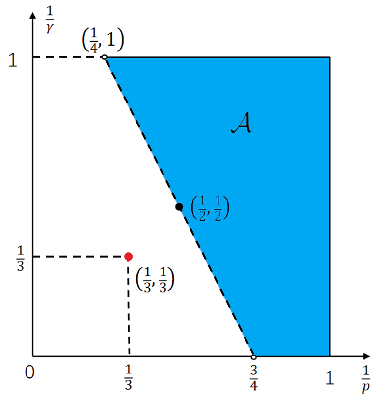
Figure 1.

(The red point is the conjectured regularity corresponding to $L^{3}_{t,x}$,

the blue region is the admissible set $\mathcal{A}$ of regularities when $s=0$.)

As a consequence, Theorem 1.2 gives the following result concerning the non-uniqueness of weak solutions and the non-conservation of magnetic helicity.

Corollary 1.3.

For any ${\alpha}_{1},{\alpha}_{2}\in[0,5/4)$ and any $(s,p,\gamma)\in\mathcal{A}$, where the regularity admissible set $\mathcal{A}$ is as in (1.5), there exist infinitely many weak solutions to (1.4) with the same data at time zero, which live in the space $H^{\beta^{\prime}}_{t,x}\cap L^{\gamma}_{t}W^{s,p}_{x}$ for some $\beta^{\prime}>0$ and do not conserve the magnetic helicity.

Remark 1.4.

(i). The non-uniqueness results for the ideal MHD (1.2) were proved by Faraco-Lindberg-Székelyhidi [36] for weak solutions with compact support in space-time, and by Beekie-Buckmaster-Vicol [2] for weak solutions with non-trivial magnetic helicity.

To the best of our knowledge, Corollary 1.3 provides the first non-uniqueness result for the weak solutions to the MHD equations (1.4) with $\alpha_{i}\in(0,5/4)$, i.e., less than the sharp Lions exponent.

(ii). By the Onsager-type conjecture for the magnetic helicity in [15], it was expected that $L^{3}_{t,x}$ is the threshold for the magnetic helicity conservation for the ideal MHD. This conjecture was solved recently by Faraco-Lindberg-Székelyhidi [37], by constructing weak solutions uniformly-in-time in the spatial Lorentz space $L^{3,\infty}_{x}$ with non-trivial magnetic helicity, based on the convex integration via staircase laminates.

In view of Corollary 1.3, one has more examples in the spaces $H^{\beta^{\prime}}_{t,x}\cap L^{\gamma}_{t}W^{s,p}_{x}$ for the flexible part of the conjecture for the magnetic helicity, where $\beta^{\prime}$ is a positive small constant and $(s,p,\gamma)\in\mathcal{A}$ with $\mathcal{A}$ as in Theorem 1.2.

(iii). In the higher dimensions $d\geq 4$, one may prove the non-uniqueness of weak solutions in $C_{t}L^{2}_{x}$ for the viscous and resistive MHD (1.1). The solutions can be continuous in time. This is possible because, in high dimensions $d\geq 4$, there is more freedom to choose the oscillation directions in the velocity and magnetic flows, which permit to gain the 3D spatial intermittency to control the Laplacian $(-\Delta)$.

(iv). We expect that the proof of this paper applies to the non-uniqueness in law for the stochastic generalized MHD equations driven by Wiener processes, which will be done in a forthcoming work. We would like to refer the reader to the papers [6, 20, 40, 39] for the recent developments in the stochastic contexts.

Our next result is concerned with the vanishing viscosity and resistivity limits of the weak solutions to (1.4).

Theorem 1.5.

Let ${\alpha}_{1},{\alpha}_{2}\in(0,5/4)$ and $(u,B)\in H^{\widetilde{\beta}}_{t,x}\times H^{\widetilde{\beta}}_{t,x}$ be any mean-free weak solution to the ideal MHD (1.2), where $\widetilde{\beta}>0$. Then, there exist $\beta^{\prime}\in(0,\widetilde{\beta})$ and a sequence of weak solutions $(u^{(\nu_{n})},B^{(\nu_{n})})\in H^{\beta^{\prime}}_{t,x}\times H^{\beta^{\prime}}_{t,x}$ to the MHD equations (1.4), where $\nu_{n}=(\nu_{1,n},\nu_{2,n})$ and $\nu_{1,n}$, $\nu_{2,n}$ are the viscosity and resistivity coefficients, respectively, such that as $\nu_{n}\rightarrow 0$,

$$u^{(\nu_{n})}\rightarrow u,\quad B^{(\nu_{n})}\rightarrow B\quad\text{strongly in}\ H^{\beta^{\prime}}_{t,x}.$$ (1.6)

Remark 1.6.

(i). By Theorem 1.5, the set of the accumulation points of weak solutions to the MHD equations (1.4), in the $H^{\beta^{\prime}}_{t,x}$ topology, contains the weak solutions to the ideal MHD equations (1.2). This extends the vanishing viscosity result in the context of the NSE [13] to the MHD equations up to the Lions exponent.

Let us mention that, the Sobolev space $H^{\widetilde{\beta}}_{t,x}$ is less regular than $C^{\widetilde{\beta}}_{t,x}$ used in the vanishing viscosity limit result for the NSE in [13]. In order to get the temporal regularity of solutions, we use the Slobodetskii-type norm of $H^{\widetilde{\beta}}_{t,x}$ to gain the regularity on average, which turns out to be efficient to prove the vanishing viscosity limit in the Sobolev space $H^{\beta^{\prime}}_{t,x}$ with $\beta^{\prime}<\widetilde{\beta}$. See the proof of (6.35) and (6.3) below.

(ii). Another interesting outcome of Theorem 1.5 is related to the weak solutions constructed in [2] and to the Taylor conjecture concerning the conservation of magnetic helicity.

The Taylor conjecture is mathematically formulated in the concept of weak ideal limits, i.e., the weak limits of Leray weak solutions, and has been recently proved by Faraco-Lindberg [35]. The crucial ingredient of the proof is the regularity of Leray approximating solutions. Hence, the weak solutions constructed in [2] with non-trivial magnetic helicity cannot be obtained as the weak ideal limits of Leray-Hopf solutions to the MHD (1.1) (cf. [2, 15]).

Let us mention that, the weak solutions constructed in [2] has the regularity $H^{\widetilde{\beta}}_{t,x}$ for some $\widetilde{\beta}>0$ (see Remark 6.1 below). Hence, by virtue of Theorem 1.5, we note that, in contrast to the weak ideal limits, the weak solutions in [2] actually can be obtained as the vanishing viscosity and resistivity limits of those to the MHD equations (1.4), where the exponents ${\alpha}_{i}$ can be even larger than one. In particular, this yields that Taloy’s conjecture does not hold along the vanishing viscosity and resistivity limits of the weak solutions to (1.4).

1.3. Outline of the proof

Our strategy of proof is based on the intermittent convex integration scheme, inspired by the works [2, 13, 19].

More precisely, for each integer $q\in\mathbb{N}$, we consider the following relaxation system

$$\left\{\begin{aligned} &\partial_{t}{u_{q}}+\nu_{1}(-\Delta)^{\alpha_{1}}{u_{q}}+{\mathrm{div}}({u_{q}}\otimes{u_{q}}-{B_{q}}\otimes{B_{q}})+\nabla P_{q}={\mathrm{div}}\mathring{R}_{q}^{u},\\ &\partial_{t}{B_{q}}+\nu_{2}(-\Delta)^{\alpha_{2}}{B_{q}}+{\mathrm{div}}({B_{q}}\otimes{u_{q}}-{u_{q}}\otimes{B_{q}})={\mathrm{div}}\mathring{R}_{q}^{B},\\ &{\mathrm{div}}{u_{q}}=0,\quad{\mathrm{div}}{B_{q}}=0,\end{aligned}\right.$$ (1.7)

where the Reynolds stress $\mathring{R}_{q}^{u}$ is a symmetric traceless $3\times 3$ matrix, and the magnetic stress $\mathring{R}_{q}^{B}$ is a skew-symmetric $3\times 3$ matrix.

The quantitative estimates of the relaxation solutions $(u_{q},B_{q},\mathring{R}^{u}_{q},\mathring{R}^{B}_{q})$ are specified in the main iteration result below.

More precisely, let $\alpha:=\max\{\alpha_{1},\alpha_{2}\}$, $\alpha_{*}:=\max\{2\alpha-1,0\}$. Take $\varepsilon\in\mathbb{Q}_{+}$ sufficiently small such that

$$\varepsilon\leq\min\left\{\frac{3-2\alpha_{*}}{20},\frac{1}{10}\right\},$$ (1.8)

and

$$s+\frac{3}{2}-\frac{2}{p}-\frac{1}{\gamma}+8{\varepsilon}<0.$$ (1.9)

For $q\in\mathbb{N}$, the frequency parameter $\lambda_{q}$ and the amplitude parameter $\delta_{q+2}$ are defined by

$$\lambda_{q}=a^{(b^{q})},\ \ \delta_{q+2}=\lambda_{q+2}^{-2\beta}.$$ (1.10)

Here, $a\in 5\mathbb{N}$ is a large integer of multiple $5$ such that $a^{\varepsilon}\in 5\mathbb{N}$, $b\in 2\mathbb{N}$ is a large integer of multiple $2$ such that $\lambda_{q+1}^{2\varepsilon}=\lambda_{q}^{2\varepsilon b}\in\mathbb{N}$ and

$$b>\frac{1000}{\varepsilon},\ \ 0<\beta<\frac{1}{100b^{2}}.$$ (1.11)

Let $q\in\mathbb{N}$, we assume the following inductive estimates of the relexation solutions to (1.7) at level $q$:

$$\|{u_{q}}\|_{C_{t,x}^{1}}\leq\lambda_{q}^{7},\quad\|{B_{q}}\|_{C_{t,x}^{1}}\leq\lambda_{q}^{7},$$ (1.12)

$$\|\mathring{R}_{q}^{u}\|_{C^{1}_{t,x}}\leq\lambda_{q}^{14},\quad\|\mathring{R}_{q}^{B}\|_{C^{1}_{t,x}}\leq\lambda_{q}^{14},$$ (1.13)

$$\|\mathring{R}_{q}^{u}\|_{L^{1}_{t,x}}\leq\delta_{q+1},\quad\|\mathring{R}_{q}^{B}\|_{L^{1}_{t,x}}\leq\delta_{q+1}.$$ (1.14)

The main iteration result is contained in the following theorem.

Theorem 1.7 (Main iteration).

Let $\alpha_{1},\alpha_{2}\in[0,5/4)$. Then, there exist $\beta\in(0,1)$, $M>0$ large enough and $a_{0}=a_{0}(\beta,M)$, such that for any integer $a\geq a_{0}$, the following holds:

Suppose that $({u_{q}},{B_{q}},\mathring{R}_{q}^{u},\mathring{R}_{q}^{B})$ solves (1.7) and satisfies (1.12)-(1.14). Then, there exists $(u_{q+1},B_{q+1},\mathring{R}^{u}_{q+1},\mathring{R}^{B}_{q+1})$ solving (1.7) and satisfying (1.12)-(1.14) with $q+1$ replacing $q$. In addition, we have

$$\left\|u_{q+1}-u_{q}\right\|_{L^{2}_{t,x}}\leq M\delta_{q+1}^{\frac{1}{2}},\quad\left\|B_{q+1}-B_{q}\right\|_{L^{2}_{t,x}}\leq M\delta_{q+1}^{\frac{1}{2}},$$ (1.15)

$$\left\|u_{q+1}-u_{q}\right\|_{L^{1}_{t}L^{2}_{x}}\leq\delta_{q+2}^{\frac{1}{2}},\quad\left\|B_{q+1}-B_{q}\right\|_{L^{1}_{t}L^{2}_{x}}\leq\delta_{q+2}^{\frac{1}{2}},$$ (1.16)

and

$$\mathrm{supp\,}_{t}u_{q+1}\cup\mathrm{supp\,}_{t}B_{q+1}\subseteq N_{\delta_{q+2}^{\frac{1}{2}}}\left(\mathrm{supp\,}_{t}u_{q}\cup\mathrm{supp\,}_{t}B_{q}\cup\mathrm{supp\,}_{t}\mathring{R}_{q}^{u}\cup\mathrm{supp\,}_{t}\mathring{R}_{q}^{B}\right),$$ (1.17)

$$\mathrm{supp\,}_{t}\mathring{R}_{q+1}^{u}\cup\mathrm{supp\,}_{t}\mathring{R}_{q+1}^{B}\subseteq N_{\delta_{q+2}^{\frac{1}{2}}}\left(\mathrm{supp\,}_{t}u_{q}\cup\mathrm{supp\,}_{t}B_{q}\cup\mathrm{supp\,}_{t}\mathring{R}_{q}^{u}\cup\mathrm{supp\,}_{t}\mathring{R}_{q}^{B}\right).$$ (1.18)

The heart of the proof of Theorem 1.7 is to construct suitable perturbations

$$w_{q+1}\simeq u_{q+1}-u_{q},\ \ d_{q+1}\simeq B_{q+1}-B_{q},$$

module small mollification errors, such that the corresponding nonlinear effects decrease the amplitudes of the Reynolds and magnetic stresses, in order to fulfill the above iteration procedure.

1.4. New ingredients of proof

As mentioned in §1.1, besides the intermittent velocity flows $\{W_{(k)}\}$, the intermittent magnetic flows $\{D_{(k)}\}$ are also required and shall be constructed in an appropriate way, in order to respect the geometry of MHD. This forces to limit the oscillation directions, and thus the intermittent velocity and magnetic flows do not have the 3D spatial intermittency as in the NSE case [13].

In the context of the ideal MHD (1.2), the key intermittent shear velocity flows and the intermittent shear magnetic flows were introduced of the form

$$W_{(k)}=\phi_{(k)}k_{1},\quad D_{(k)}=\phi_{(k)}k_{2},$$ (1.19)

where $\{\phi_{(k)}\}$ are the spatial concentration functions with one oscillation direction $k$, orthogonal to the other two directions $k_{1},k_{2}$. The shear flows have the almost 1D spatial intermittency, i.e.,

$$\|W_{(k)}\|_{C_{t}L^{1}_{x}}+\|D_{(k)}\|_{C_{t}L^{1}_{x}}\lesssim\lambda^{-\frac{1}{2}+{\varepsilon}},$$ (1.20)

which permits to control the fractional viscosity and resistivity $(-\Delta)^{{\alpha}_{i}}$ with ${\alpha}_{i}\in[0,1/2)$, $i=1,2$.

One of the novelties of our proof is the construction of a new class of intermittent velocity and magnetic flows adapted to the geometry of MHD, which feature the refined intermittency in both the space and time and, in particular, enable us to control the stronger viscosity and resistivity $(-\Delta)^{{\alpha}_{i}}$ with ${\alpha}_{i}\geq 1/2$, $i=1,2$.

(i) Spatial intermittent building blocks. We construct the refined intermittent velocity and magnetic flows

$$W_{(k)}=\psi_{(k_{1})}\phi_{(k)}k_{1},\quad D_{(k)}=\psi_{(k_{1})}\phi_{(k)}k_{2},$$ (1.21)

which are $({{\mathbb{T}}}/({\lambda r_{\perp}}))^{3}$-periodic and concentrate on smaller cuboids with volume $\lambda^{-3}r_{\perp}^{-3}r_{\parallel}$ in each of the cubes with side length ${2\pi}/{(\lambda r_{\perp})}$. Here, $\psi_{(k_{1})}$ and $\phi_{(k)}$ are suitable concentration functions (see (3.8) below), $r_{\parallel}$ and $r_{\perp}$ are the small constants to parameterize the spatial concentration of the building blocks, as in the intermittent jets for the NSE [14].

One nice feature of the refined flows is that, they have the almost 2D intermittency

$$\|W_{(k)}\|_{C_{t}L^{1}_{x}}+\|D_{(k)}\|_{C_{t}L^{1}_{x}}\lesssim\lambda^{-1+{\varepsilon}},$$ (1.22)

and thus enable one to control the viscosity and resistivity $(-\Delta)^{{\alpha}_{i}}$ with ${\alpha}_{i}\in[1/2,1)$, $i=1,2$. Another nice feature is that, the intersections between distinct intermittent flows concentrate on much smaller cuboids, which provide the almost 2D intermittency, i.e.,

$$\|W_{(k)}\otimes W_{(k^{\prime})}\|_{C_{t}L^{1}_{x}}\lesssim\lambda^{-1+{\varepsilon}},\quad k\neq k^{\prime},$$ (1.23)

and thus simplify the control of the nonlinearities of MHD.

Let us also mention that, unlike the one oscillation direction $k$ in (1.19) in the ideal MHD case, the building blocks $W_{(k)}$ and $D_{(k)}$ in (1.21) oscillate in two orthogonal directions $k_{1}$ and $k$. This new oscillation direction $k_{1}$ causes extra high spatial oscillations, which need to be balanced by a new temporal parameter $\mu$ in the flows and the temporal correctors $w^{(t)}_{q+1}$ and $d^{(t)}_{q+1}$. See (4.37a), (4.37b) and the important indentities (4.4.1) and (4.4.1) below.

It might be tempting to introduce one more oscillation direction $k_{2}$ in the building blocks, i.e., with the oscillation directions $(k,k_{1},k_{2})$ as in the NSE context [13, 14]. However, this causes even more high spatial oscillations, which seem not possible to be balanced by the temporal parameter $\mu$.

(ii) Temporal intermittent building blocks. The next major difficulty is to pass beyond the border line ${\alpha}_{i}=1$, $i=1,2$.

The key idea here is to exploit the new intermittency from the temporal oscillations. Thus, rather than performing the pointwise analysis in time, we measure the Reynolds and magnetic stresses on average, i.e., in the space $L^{1}_{t,x}$.

Let us mention that, this is in spirit close to the works [13, 18]. In [18] the temporal intermittency is crucial to achieve the non-uniqueness of weak solutions for transport equations at the critical space regularity. In the NSE context [13], the key ingredient is the $L^{2}_{x}$-based spatial intermittency, instead of the previous pointwise analysis in space as in the Euler settings.

We introduce the temporal concentration function $g_{(\tau)}$ in the principal part of perturbations $(w_{q+1}^{(p)}$, $d_{q+1}^{(p)})$, and control the oscillation errors in the space $L^{1}_{t}$. Here, $\tau$ is the constant to parameterize the temporal concentration. In particular, this permits to gain an additional 1D intermittency, i.e.,

$$\|g_{(\tau)}\|_{L^{1}_{t}}\lesssim\lambda^{-\frac{1}{2}+{\varepsilon}}.$$ (1.24)

More interestingly, the gained temporal intermittency enables to control the much stronger viscosity and resistivity $(-\Delta)^{{\alpha}_{i}}$ for all the exponents ${\alpha}_{i}$ less than $5/4$, $i=1,2$, that is, exactly the Lions exponent.

It should be mentioned that, extra high temporal oscillations also arise due to the presence of the temporal concentration function $g_{(\tau)}$. In order to balance these high oscillations, another new type of temporal correctors $w_{q+1}^{(o)},d_{q+1}^{(o)}$ will be introduced, respectively, for the velocity and magnetic flows. See (4.40a), (4.40b) and the key identities (4.4.2) and (4.4.2) below.

The remainder of this paper is organized as follows. We first regularize the relexation solutions to (1.7) by the standard mollification procedure in Section 2. Section 3 is devoted to the construction of the crucial intermittent velocity and magnetic flows adapted to MHD, which feature the intermittency in both the space and the time. Then, in Section 4 we construct the velocity and magnetic perturbations, consisting of the principal parts to decrease the Reynolds and magnetic stresses, the incompressibility correctors and two types of temporal correctors. Several key algebraic identities and analytic estimates also will be given there, which lead to the verification of the inductive estimates for the velocity and magnetic fields. Then, the inductive estimates of Reynolds and magnetic stresses are verified in Section 5. Consequently, the proof of the main results is presented in Section 6.

2. Mollification

In order to avoid the loss of derivatives, we mollify the velocity and magnetic fields. Let $\phi_{\varepsilon}$ and $\varphi_{\varepsilon}$ be the mollifiers on ${\mathbb{T}}^{3}$ and ${\mathbb{T}}$, respectively, ${\varepsilon}>0$, and $\mathrm{supp\,}{\varphi}_{\varepsilon}\subseteq(-{\varepsilon},{\varepsilon})$.

The mollifications of $({u_{q}},{B_{q}},\mathring{R}_{q}^{u},\mathring{R}_{q}^{B})$ in space and time are defined by

$$\begin{array}[]{ll}&u_{\ell}:=\left(u_{q}*_{x}\phi_{\ell}\right)*_{t}\varphi_{\ell},\quad B_{\ell}:=\left({B_{q}}*_{x}\phi_{\ell}\right)*_{t}\varphi_{\ell},\\ &\mathring{R}_{\ell}^{u}:=\left(\mathring{R}_{q}^{u}*_{x}\phi_{\ell}\right)*_{t}\varphi_{\ell},\quad\mathring{R}_{\ell}^{B}:=\left(\mathring{R}_{q}^{B}*_{x}\phi_{\ell}\right)*_{t}\varphi_{\ell},\end{array}$$ (2.1)

where the scale of mollification is parameterized by

$$\ell:=\lambda_{q}^{-20}.$$ (2.2)

Then, by equation (1.7), $(u_{\ell},B_{\ell},\mathring{R}_{\ell}^{u},\mathring{R}_{\ell}^{B})$ satisfies

$$\left\{\begin{aligned} &\partial_{t}u_{\ell}+\nu_{1}(-\Delta)^{\alpha_{1}}u_{\ell}+{\mathrm{div}}\left(u_{\ell}\otimes u_{\ell}-B_{\ell}\otimes B_{\ell}\right)+\nabla P_{\ell}={\mathrm{div}}(\mathring{R}_{\ell}^{u}+\mathring{R}_{com}^{u}),\\ &\partial_{t}B_{\ell}+\nu_{2}(-\Delta)^{\alpha_{2}}B_{\ell}+{\mathrm{div}}\left(B_{\ell}\otimes u_{\ell}-u_{\ell}\otimes B_{\ell}\right)={\mathrm{div}}(\mathring{R}_{\ell}^{B}+\mathring{R}_{com}^{B}),\\ &{\mathrm{div}}u_{\ell}=0,\quad{\mathrm{div}}B_{\ell}=0,\\ \end{aligned}\right.$$ (2.3)

where the traceless symmetric commutator stress $\mathring{R}_{com}^{u}$ and the skew-symmetric commutator stress $\mathring{R}_{com}^{B}$ are of form

$$\mathring{R}_{com}^{u}:=u_{\ell}\mathring{\otimes}u_{\ell}-B_{\ell}\mathring{\otimes}B_{\ell}-\left({u_{q}}\mathring{\otimes}{u_{q}}-{B_{q}}\mathring{\otimes}{B_{q}}\right)*_{x}\phi_{\ell}*_{t}\varphi_{\ell},$$ (2.4)

$$\mathring{R}_{com}^{B}:=B_{\ell}\otimes u_{\ell}-u_{\ell}\otimes B_{\ell}-\left({B_{q}}\otimes{u_{q}}-{u_{q}}\otimes{B_{q}}\right)*_{x}\phi_{\ell}*_{t}\varphi_{\ell},$$

and the pressure $P_{\ell}$ is given by

$$P_{\ell}:=\left(P_{q}*_{x}\phi_{\ell}\right)*_{t}\varphi_{\ell}-\left|u_{\ell}\right|^{2}+\left|B_{\ell}\right|^{2}+\left(\left|{u_{q}}\right|^{2}-\left|{B_{q}}\right|^{2}\right)*_{x}\phi_{\ell}*_{t}\varphi_{\ell}.$$ (2.5)

By the standard mollification estimates and the inductive estimates (1.12)-(1.14), for any $N\in\mathbb{N}_{+}$,

$$\left\|u_{\ell}\right\|_{C_{t,x}^{N}}+\left\|B_{\ell}\right\|_{C_{t,x}^{N}}\lesssim\ell^{-N+1}(\left\|u_{q}\right\|_{C_{t,x}^{1}}+\left\|B_{q}\right\|_{C_{t,x}^{1}})\lesssim\ell^{-N+1}\lambda_{q}^{7}\lesssim\ell^{-N},$$ (2.6)

$$\|\mathring{R}_{\ell}^{u}\|_{C_{t,x}^{N}}+\|\mathring{R}_{\ell}^{B}\|_{C_{t,x}^{N}}\lesssim\ell^{-N+1}(\|\mathring{R}_{q}^{u}\|_{C_{t,x}^{1}}+\|\mathring{R}_{q}^{B}\|_{C_{t,x}^{1}})\lesssim\ell^{-N+1}\lambda_{q}^{14}\lesssim\ell^{-N},$$ (2.7)

$$\|\mathring{R}_{\ell}^{u}\|_{L^{1}_{t,x}}\lesssim\delta_{q+1},\quad\|\mathring{R}_{\ell}^{B}\|_{L^{1}_{t,x}}\lesssim\delta_{q+1}.$$ (2.8)

Moreover, by the inductive estimate (1.12) and the double commutator estimate (see, e.g., [56, Proposition B.1], [24, Lemma 1], [23]), for $1<p<+{\infty}$,

$$\|\mathring{R}_{com}^{u}\|_{L^{1}_{t}L^{p}_{x}}\lesssim\|\mathring{R}_{com}^{u}\|_{C_{t,x}}\lesssim\ell(\|u_{q}\|_{C_{t,x}^{1}}^{2}+\|B_{q}\|_{C_{t,x}^{1}}^{2})\lesssim\ell\lambda_{q}^{14},$$ (2.9)

and, similarly,

$$\|\mathring{R}_{com}^{B}\|_{L^{1}_{t}L^{p}_{x}}\lesssim\|\mathring{R}_{com}^{B}\|_{C_{t,x}}\lesssim\ell\lambda_{q}^{14}.$$ (2.10)

3. Intermittent velocity and magnetic flows

This section contains the crucial intermittent velocity and magnetic flows, which are indeed the fundamental building blocks in the convex integration scheme.

We set the parameters $r_{\perp}$, $r_{\parallel}$, $\lambda$, $\mu$, $\tau$ and $\sigma$ as follows

$$r_{\perp}:=\lambda_{q+1}^{-1+2\varepsilon},\ r_{\parallel}:=\lambda_{q+1}^{-1+6\varepsilon},\ \lambda:=\lambda_{q+1},\ \mu:=\lambda_{q+1}^{\frac{3}{2}-6\varepsilon},\ \tau:=\lambda_{q+1}^{1-6\varepsilon},\ \sigma:=\lambda_{q+1}^{2\varepsilon},$$ (3.1)

where $\varepsilon$ is the small constant satisfying (1.8).

3.1. Geometric lemmas.

To begin with, let us first recall two geometric lemmas in [2].

Lemma 3.1.

(First Geometric Lemma, [2, Lemma 4.1]) There exists a set $\Lambda_{B}\subset S^{2}\cap\mathbb{Q}^{3}$ that consists of vectors $k$ with associated orthonormal bases $(k,k_{1},k_{2})$, $\varepsilon_{B}>0$, and smooth positive functions $\gamma_{(k)}:B_{\varepsilon_{B}}(0)\to\mathbb{R}$, where $B_{\varepsilon_{B}}(0)$ is the ball of radius $\varepsilon_{B}$ centered at 0 in the space of $3\times 3$ skew-symmetric matrices, such that for $A\in B_{\varepsilon_{B}}(0)$ we have the following identity:

$$A=\sum_{k\in\Lambda_{B}}\gamma_{(k)}^{2}(A)(k_{2}\otimes k_{1}-k_{1}\otimes k_{2}).$$ (3.2)

Lemma 3.2.

(Second Geometric Lemma, [2, Lemma 4.2]) There exists a set $\Lambda_{u}\subset S^{2}\cap\mathbb{Q}^{3}$ that consists of vectors $k$ with associated orthonormal bases $(k,k_{1},k_{2})$, $\varepsilon_{u}>0$, and smooth positive functions $\gamma_{(k)}:B_{\varepsilon_{u}}(\mathrm{Id})\to\mathbb{R}$, where $B_{\varepsilon_{u}}(\mathrm{Id})$ is the ball of radius $\varepsilon_{u}$ centered at the identity in the space of $3\times 3$ symmetric matrices, such that for $S\in B_{\varepsilon_{u}}(\mathrm{Id})$ we have the following identity:

$$S=\sum_{k\in\Lambda_{u}}\gamma_{(k)}^{2}(S)k_{1}\otimes k_{1}.$$ (3.3)

Furthermore, we may choose $\Lambda_{u}$ such that $\Lambda_{B}\cap\Lambda_{u}=\emptyset$.

As pointed out in [2], there exists $N_{\Lambda}\in\mathbb{N}$ such that

$$\{N_{\Lambda}k,N_{\Lambda}k_{1},N_{\Lambda}k_{2}\}\subset N_{\Lambda}\mathbb{S}^{2}\cap\mathbb{Z}^{3}.$$ (3.4)

For instance, $N_{\Lambda}=65$ suffices. We denote by $M_{*}$ the geometric constant such that

$$\sum_{k\in\Lambda_{u}}\lVert\gamma_{(k)}\rVert_{C^{4}(B_{\varepsilon_{u}}(\mathrm{Id}))}+\sum_{k\in\Lambda_{B}}\lVert\gamma_{(k)}\rVert_{{C^{4}(B_{\varepsilon_{B}}}(0))}\leq M_{*}.$$ (3.5)

This parameter is universal and will be used later in the estimates of the size of perturbations.

According to the proof of [2, Lemmas 4.1 and 4.2], we can choose the wave vectors satisfying $k_{2}\not=k_{2}^{\prime}$ if $k\not=k^{\prime}$, so that the intersections between distinct intermittent flows concentrate on much smaller cuboids and have 2D spatial intermittency (see Lemma 3.4 below).

3.2. Spatial building blocks.

Let $\Phi:\mathbb{R}\to\mathbb{R}$ be a smooth cut-off function supported on the interval $[-1,1]$. We normalize $\Phi$ such that $\phi:=-\frac{d^{2}}{dx^{2}}\Phi$ satisfies

$$\frac{1}{2\pi}\int_{\mathbb{R}}\phi^{2}(x){\rm d}x=1.$$ (3.6)

Moreover, let $\psi:\mathbb{R}\rightarrow\mathbb{R}$ be a smooth and mean zero function, supported on the interval $[-1,1]$, satisfying

$$\frac{1}{2\pi}\int_{\mathbb{R}}\psi^{2}\left(x\right){\rm d}x=1.$$ (3.7)

The corresponding rescaled cut-off functions are defined by

$$\phi_{r_{\perp}}(x):={r_{\perp}^{-\frac{1}{2}}}\phi\left(\frac{x}{r_{\perp}}\right),\quad\Phi_{r_{\perp}}(x):={r_{\perp}^{-\frac{1}{2}}}\Phi\left(\frac{x}{r_{\perp}}\right),\quad\psi_{r_{\parallel}}\left(x\right):={r_{\|}^{-\frac{1}{2}}}\psi\left(\frac{x}{r_{\|}}\right).$$

Note that, $\phi_{r_{\perp}}=-r_{\perp}^{2}\frac{d^{2}}{dx^{2}}\Phi_{r_{\perp}}$, and $\phi_{r_{\perp}},\psi_{r_{\parallel}}$ are supported in the ball of radius $r_{\perp}$ and $r_{\parallel}$, respectively, in ${\mathbb{R}}$. By an abuse of notation, we periodize $\phi_{r_{\perp}}$, $\Phi_{r_{\perp}}$ and $\psi_{r_{\parallel}}$ so that they are treated as periodic functions defined on $\mathbb{T}$.

The intermittent velocity flows are defined by

$$W_{(k)}:=\psi_{r_{\parallel}}(\lambda r_{\perp}N_{\Lambda}(k_{1}\cdot x+\mu t))\phi_{r_{\perp}}(\lambda r_{\perp}N_{\Lambda}k\cdot x)k_{1},\ \ k\in\Lambda_{u}\cup\Lambda_{B},$$

and the intermittent magnetic flows are defined by

$$D_{(k)}:=\psi_{r_{\parallel}}(\lambda r_{\perp}N_{\Lambda}(k_{1}\cdot x+\mu t))\phi_{r_{\perp}}(\lambda r_{\perp}N_{\Lambda}k\cdot x)k_{2},\ \ k\in\Lambda_{B}.$$

Here, $N_{\Lambda}$ is given by (3.4) above, $(k,k_{1},k_{2})$ are the orthonormal bases in ${\mathbb{R}}^{3}$ in Lemmas 3.1 and 3.2. The parameters $r_{\parallel}$ and $r_{\perp}$ parameterize the concentration of the flows, and $\mu$ is the temporal oscillation parameter.

By definition, $\{W_{(k)},D_{(k)}\}$ are $(\mathbb{T}/(\lambda r_{\perp}))^{3}$-periodic, supported on thin cuboids with length $\sim{1}/{\lambda r_{\perp}}$, width $\sim{r_{\parallel}}/{(\lambda r_{\perp})}$ and height $\sim{1}/{\lambda}$. See the intermittent flows in Figure 2. See also the analytic properties in Lemma 3.3 below.

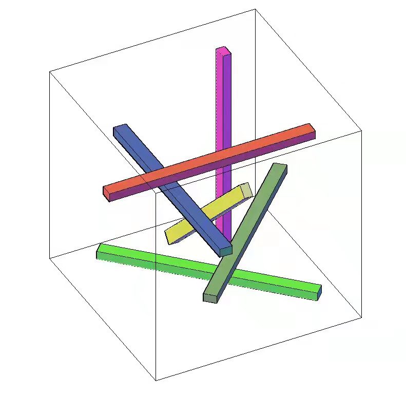
Figure 2. Intermittent flows

Moreover, as there are only finite number of vectors in the wavevector sets $\Lambda_{u}$ and $\Lambda_{B}$, by choosing $k_{2}\neq k_{2}^{\prime}$ if $k\neq k^{\prime}$, we note that the intersections of distinct intermittent flows have much smaller volume. See Figure 3 below for the typical cases of intersections, and Lemma 3.4 below for the corresponding analytic properties.

(a) Case 1

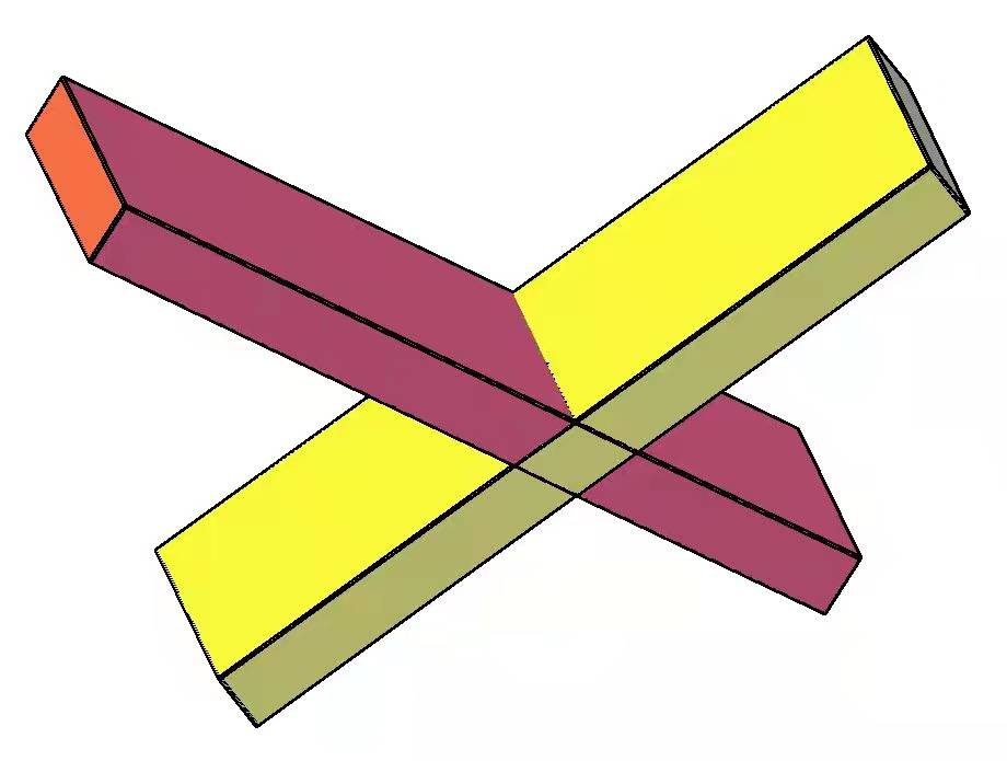
(b) Case 2

Figure 3. Typical cases of intersections

To ease notations, we set

$$\begin{array}[]{ll}&\phi_{(k)}(x):=\phi_{r_{\perp}}(\lambda r_{\perp}N_{\Lambda}k\cdot x),\ \ \Phi_{(k)}(x):=\Phi_{r_{\perp}}(\lambda r_{\perp}N_{\Lambda}k\cdot x),\\ &\psi_{(k_{1})}(x):=\psi_{r_{\parallel}}(\lambda r_{\perp}N_{\Lambda}(k_{1}\cdot x+\mu t)),\end{array}$$ (3.8)

and thus

$$W_{(k)}=\psi_{(k_{1})}\phi_{(k)}k_{1},\ k\in\Lambda_{u}\cup\Lambda_{B},\ \ \ D_{(k)}=\psi_{(k_{1})}\phi_{(k)}k_{2},\ k\in\Lambda_{B}.$$ (3.9)

Note that, $W_{(k)}$ and $D_{(k)}$ are mean zero on ${\mathbb{T}}^{3}$. Moreover, since

$${\fint}_{\mathbb{T}^{3}}\phi_{(k)}^{2}(x){\rm d}x=1,\quad\text{and}\quad{\fint}_{\mathbb{T}^{3}}\psi_{(k_{1})}^{2}(x){\rm d}x=1,$$ (3.10)

it follows that

$$\begin{array}[]{ll}&\displaystyle{\fint}_{\mathbb{T}^{3}}W_{(k)}\otimes W_{(k)}{\rm d}x=k_{1}\otimes k_{1},\ \ {\fint}_{\mathbb{T}^{3}}D_{(k)}\otimes D_{(k)}{\rm d}x=k_{2}\otimes k_{2},\end{array}$$ (3.11)

$$\begin{array}[]{ll}&\displaystyle{\fint}_{\mathbb{T}^{3}}W_{(k)}\otimes D_{(k)}{\rm d}x=k_{1}\otimes k_{2},\ \ {\fint}_{\mathbb{T}^{3}}D_{(k)}\otimes W_{(k)}{\rm d}x=k_{2}\otimes k_{1}.\end{array}$$ (3.12)

It is worth noting that, the building blocks in [2] have one oscillation direction $k$, orthogonal to the direction vectors $k_{1}$ and $k_{2}$, and have the 1D intermittency.

In order to control the stronger viscosity and resistivity $(-\Delta)^{{\alpha}_{i}}$ when ${\alpha}_{i}\geq 1/2$, $i=1,2$, the idea here to explore more intermittency, inspired by the work [13] in the NSE context, is to introduce the new concentration function $\psi_{(k_{1})}$ in (3.9). Two new parameters $r_{\perp}$ (the rescaling parameter in the direction vertical to the flow) and $r_{\parallel}$ (the rescaling parameter in the direction parallel to the flow) parameterize the concentration of the intermittent flows $W_{(k)}$ and $D_{(k)}$. In particular, one has

$$\sum\limits_{k\in\Lambda_{u}\cup\Lambda_{B}}\|W_{(k)}\|_{C_{t}L^{1}_{x}}+\sum\limits_{k\in\Lambda_{B}}\|D_{(k)}\|_{C_{t}L^{1}_{x}}\lesssim r_{\perp}^{\frac{1}{2}}r_{\parallel}^{\frac{1}{2}}=\lambda_{q+1}^{-1+4{\varepsilon}},$$ (3.13)

which gives the almost $2D$ intermittency and thus permits to control the fractional viscosity and resistivity $(-\Delta)^{{\alpha}_{i}}$ in (1.4) for any ${\alpha}_{1},{\alpha}_{2}\in[0,1)$.

Furthermore, the new parameter $\mu$ permits to control the temporal correctors later to balance the high spatial oscillations, arising from the concentration function $\psi_{(k)}.$ More precisely, using the orthogonality

$$\begin{array}[]{ll}&\nabla\phi_{(k)}\cdot k_{1}=\nabla\phi_{(k)}\cdot k_{2}=0,\\ &\nabla\psi_{(k_{1})}\cdot k=\nabla\psi_{(k_{1})}\cdot k_{2}=0,\end{array}$$ (3.14)

we have the important algebraic identities

$$\begin{array}[]{ll}&\displaystyle{\mathrm{div}}(W_{(k)}\otimes W_{(k)})=2(W_{(k)}\cdot\nabla\psi_{(k_{1})})\phi_{(k)}k_{1}=\frac{1}{\mu}\partial_{t}\left(\psi_{(k_{1})}^{2}\phi_{(k)}^{2}k_{1}\right),\\ &\displaystyle{\mathrm{div}}(D_{(k)}\otimes D_{(k)})=2(D_{(k)}\cdot\nabla\psi_{(k_{1})})\phi_{(k)}k_{2}=0,\end{array}$$ (3.15)

and

$$\begin{array}[]{ll}&\displaystyle{\mathrm{div}}(D_{(k)}\otimes W_{(k)})=({\mathrm{div}}W_{(k)})D_{(k)}+(W_{(k)}\cdot\nabla)D_{(k)}=\frac{1}{\mu}\partial_{t}\left(\psi_{(k_{1})}^{2}\phi_{(k)}^{2}k_{2}\right),\\ &\displaystyle{\mathrm{div}}(W_{(k)}\otimes D_{(k)})=({\mathrm{div}}D_{(k)})W_{(k)}+(D_{(k)}\cdot\nabla)W_{(k)}=0.\end{array}$$ (3.16)

Thus, when combining with the temporal correctors, module a pressure term, the time derivative can be moved onto the low oscillating amplitudes (see (4.4.1), (4.4.1) below).

Because the intermittent flow $W_{(k)}$ is not divergence-free, we also need the corrector

$$\widetilde{W}_{(k)}^{c}:=\frac{1}{\lambda^{2}N_{\Lambda}^{2}}\nabla\psi_{(k_{1})}\times{\mathrm{curl}}(\Phi_{(k)}k_{1}).$$ (3.17)

Then, straightforward computations show that

$$W_{(k)}+\widetilde{W}_{(k)}^{c}={\mathrm{curl}}{\mathrm{curl}}\left(\frac{1}{\lambda^{2}N_{\Lambda}^{2}}\psi_{(k_{1})}\Phi_{(k)}k_{1}\right)={\mathrm{curl}}{\mathrm{curl}}W^{c}_{(k)},$$ (3.18)

where $W^{c}_{(k)}$ is given by

$$W^{c}_{(k)}:=\frac{1}{\lambda^{2}N_{\Lambda}^{2}}\psi_{(k_{1})}\Phi_{(k)}k_{1}.$$ (3.19)

Thus, it follows that

$${\mathrm{div}}(W_{(k)}+\widetilde{W}^{c}_{(k)})=0.$$ (3.20)

Regarding the magnetic flows, we introduce the correctors

$$D_{(k)}^{c}:=\frac{1}{\lambda^{2}N_{\Lambda}^{2}}\psi_{(k_{1})}\Phi_{(k)}k_{2},\quad\widetilde{D}_{(k)}^{c}:=-\frac{1}{\lambda^{2}N_{\Lambda}^{2}}\Delta\psi_{(k_{1})}\Phi_{(k)}k_{2},\quad k\in\Lambda_{B}.$$ (3.21)

It holds that

$$D_{(k)}+\widetilde{D}_{(k)}^{c}={\mathrm{curl}}{\mathrm{curl}}D^{c}_{(k)}.$$ (3.22)

Lemma 3.3 below contains the key estimates of the intermittent velocity and magnetic flows.

Lemma 3.3 (Estimates of spatial intermittency).

For $p\in[1,+\infty]$, $N,\,M\in\mathbb{N}$, we have

$$\left\|\nabla^{N}\partial_{t}^{M}\psi_{(k_{1})}\right\|_{C_{t}L^{p}_{x}}\lesssim r_{\|}^{\frac{1}{p}-\frac{1}{2}}\left(\frac{r_{\perp}\lambda}{r_{\|}}\right)^{N}\left(\frac{r_{\perp}\lambda\mu}{r_{\|}}\right)^{M},$$ (3.23)

$$\left\|\nabla^{N}\phi_{(k)}\right\|_{L^{p}_{x}}+\left\|\nabla^{N}\Phi_{(k)}\right\|_{L^{p}_{x}}\lesssim r_{\perp}^{\frac{1}{p}-\frac{1}{2}}\lambda^{N},$$ (3.24)

where the implicit constants are independent of $r_{\perp},\,r_{\parallel},\,\lambda$ and $\mu$. In particular, we have

$$\displaystyle\left\|\nabla^{N}\partial_{t}^{M}W_{(k)}\right\|_{C_{t}L^{p}_{x}}+\frac{r_{\|}}{r_{\perp}}\left\|\nabla^{N}\partial_{t}^{M}\widetilde{W}_{(k)}^{c}\right\|_{C_{t}L^{p}_{x}}+\lambda^{2}\left\|\nabla^{N}\partial_{t}^{M}W_{(k)}^{c}\right\|_{C_{t}L^{p}_{x}}\displaystyle$$

$$\qquad\lesssim r_{\perp}^{\frac{1}{p}-\frac{1}{2}}r_{\|}^{\frac{1}{p}-\frac{1}{2}}\lambda^{N}\left(\frac{r_{\perp}\lambda\mu}{r_{\|}}\right)^{M},\ \ k\in\Lambda_{u}\cup\Lambda_{B},$$ (3.25)

$$\displaystyle\left\|\nabla^{N}\partial_{t}^{M}D_{(k)}\right\|_{C_{t}L^{p}_{x}}+\frac{r_{\|}}{r_{\perp}}\left\|\nabla^{N}\partial_{t}^{M}\widetilde{D}_{(k)}^{c}\right\|_{C_{t}L^{p}_{x}}+\lambda^{2}\left\|\nabla^{N}\partial_{t}^{M}D_{(k)}^{c}\right\|_{C_{t}L^{p}_{x}}$$

$$\qquad\lesssim r_{\perp}^{\frac{1}{p}-\frac{1}{2}}r_{\|}^{\frac{1}{p}-\frac{1}{2}}\lambda^{N}\left(\frac{r_{\perp}\lambda\mu}{r_{\|}}\right)^{M},\ \ k\in\Lambda_{B}.$$ (3.26)

Proof.

By the definitions of $\psi_{(k_{1})}$, $\phi_{(k)}$ and $\Phi_{(k)}$, the $L^{\infty}$-norms can be bounded by

$$\left\|\nabla^{N}\partial_{t}^{M}\psi_{(k_{1})}\right\|_{C_{t,x}}\lesssim r_{\|}^{-\frac{1}{2}}\left(\frac{r_{\perp}\lambda}{r_{\|}}\right)^{N}\left(\frac{r_{\perp}\lambda\mu}{r_{\|}}\right)^{M},$$ (3.27)

$$\left\|\nabla^{N}\phi_{(k)}\right\|_{L^{\infty}_{x}}+\left\|\nabla^{N}\Phi_{(k)}\right\|_{L^{\infty}_{x}}\lesssim\lambda^{N}r_{\perp}^{-\frac{1}{2}}.$$ (3.28)

In order to control the $L^{p}$-norm, $1\leq p<+{\infty}$, let us estimate the volume of the support of $\psi_{(k_{1})}$ below. As $\psi_{(k_{1})}$ is $(\mathbb{T}/(\lambda r_{\perp})^{3})$-periodic, it suffices to estimate the volume of the support of $\psi_{(k_{1})}$ on the cubes with side length $2\pi/(\lambda r_{\perp})$ and then multiply the resulting estimate by $(\lambda r_{\perp})^{3}$. One may let the oscillation parameter $\mu=0$ without changing the volume of the support of $\psi_{(k_{1})}$.

In each one of these cubes, $\psi_{(k_{1})}$ is supported on at most $2N_{\Lambda}$ thickened planes with thickness $\sim{r_{\parallel}}/{(\lambda r_{\perp})}$, which are parallel to each other and perpendicular to the direction $k_{1}$. Hence, the volume of the support of $\psi_{(k_{1})}$ on $\mathbb{T}^{3}$ can be bounded by

$$|\mathrm{supp\,}\psi_{(k_{1})}|\lesssim(\lambda r_{\perp})^{-2}\frac{r_{\parallel}}{\lambda r_{\perp}}(\lambda r_{\perp})^{3}\lesssim r_{\parallel}.$$ (3.29)

This along with (3.27) yields that

$$\|\nabla^{N}\partial_{t}^{M}\psi_{(k_{1})}\|_{C_{t}L^{p}_{x}}\lesssim |\mathrm{supp\,}\psi_{(k_{1})}|^{\frac{1}{p}}\,\left\|\nabla^{N}\partial_{t}^{M}\psi_{(k_{1})}\right\|_{C_{t}L^{\infty}_{x}}$$

$$\lesssim r_{\parallel}^{\frac{1}{p}-\frac{1}{2}}\left(\frac{r_{\perp}\lambda}{r_{\parallel}}\right)^{N}\left(\frac{r_{\perp}\lambda\mu}{r_{\parallel}}\right)^{M}.$$ (3.30)

Since there are only finite wavevectors in $\Lambda_{u}$ and $\Lambda_{B}$, the implicit constant can be taken independent of $k_{1}$ by taking the maximum over the wavevector sets $\Lambda_{u}$ and $\Lambda_{B}$. Thus, (3.23) is verified.

Estimate (3.24) can be proved similarly. Actually, in each of the cubic with length $2\pi/(\lambda r_{\perp})$, $\phi_{(k)}$ is supported on at most $2N_{\Lambda}$ thickened planes with thickness $\sim\lambda^{-1}$, perpendicular to the direction $k$. Hence,

$$|\mathrm{supp\,}\phi_{(k)}|\lesssim(\lambda r_{\perp})^{-2}\lambda^{-1}(\lambda r_{\perp})^{3}\lesssim r_{\perp},$$

which along with (3.28) yields that

$$\|{\nabla}^{N}\phi_{(k)}\|_{L^{p}_{x}}\lesssim|\mathrm{supp\,}\phi_{(k)}|^{\frac{1}{p}}\|{\nabla}^{N}\phi_{(k)}\|_{L^{\infty}_{x}}\lesssim r_{\perp}^{\frac{1}{p}}\lambda^{N}r_{\perp}^{-\frac{1}{2}}\lesssim r_{\perp}^{\frac{1}{p}-\frac{1}{2}}\lambda^{N}.$$

Thus, (3.24) is verified.

Finally, estimates (3.25) and (3.26) follow from (3.23), (3.24) and Fubini’s theorem. ∎

The following lemma illustrates that, more intermittency can be gained for the interactions betweens different intermittent building blocks. Intuitively, the supports of intermittent building blocks can be regarded as thin cuboids, because $k_{2}\not=k_{2}^{\prime}$ for different wavevectors, the intersection of two nonparallel thin cuboids has much smaller support.

Lemma 3.4 (Product estimate).

For $k\neq k^{\prime}\in\Lambda_{u}\cup\Lambda_{B}$ and $p\in[1,\infty]$, we have

$$\|\psi_{(k_{1})}\phi_{(k)}\psi_{(k^{\prime}_{1})}\phi_{(k^{\prime})}\|_{C_{t}L^{p}_{x}}\lesssim r_{\perp}^{\frac{1}{p}-1}r_{\parallel}^{\frac{2}{p}-1},$$ (3.31)

where the implicit constants are independent of the parameters $r_{\perp},\,r_{\parallel}$ and $\lambda$.

Proof.

As in the proof of Lemma 3.3, let us start with the $L^{\infty}$-estimate. By (3.8),

$$\|\psi_{(k_{1})}\phi_{(k)}\psi_{(k^{\prime}_{1})}\phi_{(k^{\prime})}\|_{C_{t,x}}\lesssim r_{\perp}^{-1}r_{\parallel}^{-1}.$$ (3.32)

Next, we estimate the volume of the support of $\psi_{(k_{1})}\phi_{(k)}\psi_{(k^{\prime}_{1})}\phi_{(k^{\prime})}$. As $\psi_{(k_{1})}\phi_{(k)}\psi_{(k^{\prime}_{1})}\phi_{(k^{\prime})}$ is $(\mathbb{T}/\lambda r_{\perp})^{3}$-periodic, it suffices to consider the support on the small cubes with side length $2\pi/\lambda r_{\perp}$ and then multiply the result by $(\lambda r_{\perp})^{3}$.

In each of these cubes, the support of $\psi_{(k_{1})}\phi_{(k)}$ consists of at most $2N_{\Lambda}$ parallel thin cuboids with length $\sim(\lambda r_{\perp})^{-1}$, width $\displaystyle\sim{r_{\parallel}}{(\lambda r_{\perp})^{-1}}$ and height $\sim\lambda^{-1}$. Note that, the width and height is much smaller than the length. Since $k_{2}\not=k_{2}^{\prime}$, the intersections between different supports of $\psi_{(k_{1})}\phi_{(k)}$ and $\psi_{(k_{1}^{\prime})}\phi_{(k^{\prime})}$ are contained in much smaller cuboids, with the length and width bounded by $\displaystyle\sim{r_{\parallel}}{(\lambda r_{\perp})^{-1}}$ and with the height $\sim\lambda^{-1}$. As there are at most $2N_{\Lambda}$ cuboids in the support of $\psi_{(k_{1})}\phi_{(k)}$, the number of intersections for two distinct cuboids is at most $4N_{\Lambda}^{2}$. Thus, the volume of the support of $\psi_{(k_{1})}\phi_{(k)}\psi_{(k^{\prime}_{1})}\phi_{(k^{\prime})}$ is bounded by

$$|\mathrm{supp\,}(\psi_{(k_{1})}\phi_{(k)}\psi_{(k^{\prime}_{1})}\phi_{(k^{\prime})})|\lesssim r_{\parallel}^{2}(\lambda r_{\perp})^{-2}\lambda^{-1}(\lambda r_{\perp})^{3}\lesssim r_{\parallel}^{2}r_{\perp}.$$ (3.33)

The implicit constant can be taken independent of $k_{1}$ and $k_{1}^{\prime}$, as there are only finitely many vectors in the wavevector sets $\Lambda_{u}$ and $\Lambda_{B}$.

Therefore, by virtue of (3.32) and (3.33), we arrive at

$$\|\psi_{(k_{1})}\phi_{(k)}\psi_{(k^{\prime}_{1})}\phi_{(k^{\prime})}\|_{C_{t}L^{p}_{x}}\leq \sup_{t}|\mathrm{supp\,}\,(\psi_{(k_{1})}\phi_{(k)}\psi_{(k^{\prime}_{1})}\phi_{(k^{\prime})})|^{\frac{1}{p}}\,\|\psi_{(k_{1})}\phi_{(k)}\psi_{(k^{\prime}_{1})}\phi_{(k^{\prime})}\|_{C_{t,x}}$$

$$\lesssim r_{\perp}^{\frac{1}{p}-1}r_{\parallel}^{\frac{2}{p}-1},$$ (3.34)

which yields (3.31) and finishes the proof. ∎

3.3. Temporal building blocks.

As mentioned in Section 1, the previous construction of intermittent velocity and magnetic flows cannot provide us with enough intermittency to handle the stronger viscosity and resistivity $(-\Delta)^{{\alpha}_{i}}$ when ${\alpha}_{i}\in[1,5/4)$, $i=1,2$.

The key idea here is to exploit more intermittency from temporal oscillations. Two new parameters $\tau$ and $\sigma$ will be introduced to parameterize the concentrations of the temporal function.

More precisely, let $g\in C_{c}^{\infty}({\mathbb{T}})$ be any cut-off function such that

$${\fint}_{{\mathbb{T}}}g^{2}(t){\rm d}t=1.$$

Let $\tau\in\mathbb{N}_{+}$ and rescale the cut-off function $g$ by

$$g_{\tau}(t)=\tau^{\frac{1}{2}}g(\tau t).$$ (3.35)

Then, we periodize $g_{\tau}$ such that the resulting functions (by an abuse of notion, still denoted by $g_{\tau}$) are ${\mathbb{T}}-$periodic functions.

In order to construct the temporal correctors $w_{q+1}^{(o)}$ and $d_{q+1}^{(o)}$ (see (4.40a)-(4.40b)) to balance the high temporal oscillations arising from the concentration function $g_{(\tau)}$, we also need the function $h_{\tau}:\mathbb{T}\to{\mathbb{R}}$, defined by

$$h_{\tau}(t):=\int_{-\pi}^{t}\left(g_{\tau}^{2}(s)-1\right)\ ds.$$ (3.36)

Set

$$g_{(\tau)}:=g_{\tau}(\sigma t),\ \ h_{(\tau)}(t):=h_{\tau}(\sigma t).$$ (3.37)

Note that, $h_{(\tau)}$ has the uniform $L_{t}^{\infty}$-bound

$$\|h_{(\tau)}\|_{L_{t}^{\infty}({\mathbb{T}})}\leq 1.$$ (3.38)

Moreover, we have the following temporal intermittent estimates of $g_{(\tau)}$.

Lemma 3.5 (Estimates of temporal intermittency).

For $\gamma\in[1,+\infty]$, $M\in\mathbb{N}$, we have

$$\left\|\partial_{t}^{M}g_{(\tau)}\right\|_{L^{\gamma}_{t}}\lesssim\sigma^{M}\tau^{M+\frac{1}{2}-\frac{1}{\gamma}},$$ (3.39)

where the implicit constants are independent of $\tau$ and $\sigma$.

Proof.

As in the proof of Lemma 3.3, we first estimate the $L^{\infty}$-norm of $g_{(\tau)}$. By definition,

$$\left\|\partial_{t}^{M}g_{(\tau)}\right\|_{L^{{\infty}}_{t}({\mathbb{T}})}\lesssim\sigma^{M}\tau^{M+\frac{1}{2}}.$$ (3.40)

Next, we give a bound on the volume of the support of $g_{(\tau)}$ on ${\mathbb{T}}$. Since $g_{(\tau)}$ is ${\mathbb{T}}/\sigma$-periodic, it is sufficient to obtain the estimate on the interval $[-\pi/\sigma,\pi/\sigma]$ and then multiply the result by $\sigma$. Note that, in the interval $[-\pi/\sigma,\pi/\sigma]$, $g_{(\tau)}$ is supported on an interval with length $\sim(\sigma\tau)^{-1}$, and thus the volume of the support of $g_{(\tau)}$ on ${\mathbb{T}}$ is bounded by

$$|\mathrm{supp\,}g_{(\tau)}|\lesssim(\sigma\tau)^{-1}\sigma\lesssim\tau^{-1}.$$ (3.41)

Combining (3.40) and (3.41) together we obtain

$$\|\partial_{t}^{M}g_{(\tau)}\|_{L^{\gamma}_{t}}\lesssim|\mathrm{supp\,}g_{(\tau)}|^{\frac{1}{\gamma}}\left\|\partial_{t}^{M}g_{(\tau)}\right\|_{L^{\infty}_{t}({\mathbb{T}})}\lesssim\sigma^{M}\tau^{M+\frac{1}{2}-\frac{1}{\gamma}}.$$ (3.42)

Therefore, estimate (3.39) is proved. ∎

4. Velocity and magnetic perturbations

This section is devoted to the construction of the key velocity and magnetic perturbations, including the principal parts, the incompressibility correctors, the spatial and temporal correctors. To begin with, let us first define suitable amplitudes of perturbations, which are the key to decrease the effects of old velocity and magnetic stresses.

4.1. Amplitudes

4.1.1. The magnetic amplitudes.

Let $\chi:[0,+\infty)\to\mathbb{R}$ be a smooth cut-off function such that

$$\chi(z)=\left\{\begin{aligned} &1,\quad 0\leq z\leq 1,\\ &z,\quad z\geq 2,\end{aligned}\right.$$ (4.1)

and

$$\frac{1}{2}z\leq\chi(z)\leq 2z\quad\text{for}\quad z\in(1,2).$$ (4.2)

Set

$$\rho_{B}(t,x):=2\varepsilon_{B}^{-1}\delta_{q+1}\chi\left(\frac{|\mathring{R}_{\ell}^{B}(t,x)|}{\delta_{q+1}}\right),$$ (4.3)

where $\varepsilon_{B}$ is the small radius in the geometric Lemma 3.1. Then, by (4.1), (4.2) and (4.3),

$$\left|\frac{\mathring{R}_{\ell}^{B}}{\rho_{B}}\right|=\left|\frac{\mathring{R}_{\ell}^{B}}{2\varepsilon_{B}^{-1}\delta_{q+1}\chi(\delta_{q+1}^{-1}|\mathring{R}_{\ell}^{B}|)}\right|\leq\varepsilon_{B},$$ (4.4)

and for any $p\in[1,+\infty]$,

$$\rho_{B}\geq\varepsilon_{B}^{-1}\delta_{q+1},$$ (4.5)

$$\lVert\rho_{B}\rVert_{L^{p}_{t,x}}\leq 8\varepsilon_{B}^{-1}\left((16\pi^{4})^{\frac{1}{p}}\delta_{q+1}+\lVert\mathring{R}_{\ell}^{B}\rVert_{L^{p}_{t,x}}\right).$$ (4.6)

Furthermore, by the standard Hölder estimate (see [10, (130)]), the iterative estimate (1.13) and (4.5), for $1\leq N\leq 4$,

$$\lVert\rho_{B}\rVert_{C_{t,x}}\lesssim\ell^{-1},\quad\lVert\rho_{B}\rVert_{C_{t,x}^{N}}\lesssim\ell^{-N}\delta^{-N+1}_{q+1},$$ (4.7)

$$\lVert\rho_{B}^{1/2}\rVert_{C_{t,x}}\lesssim\ell^{-1},\quad\lVert\rho_{B}^{1/2}\rVert_{C_{t,x}^{N}}\lesssim\ell^{-N}\delta^{-2N}_{q+1},$$ (4.8)

$$\lVert\rho_{B}^{-1}\rVert_{C_{t,x}}\lesssim\delta_{q+1}^{-1},\quad\lVert\rho_{B}^{-1}\rVert_{C_{t,x}^{N}}\lesssim\ell^{-N}\delta^{-2N}_{q+1}.$$ (4.9)

Moreover, we choose the smooth temporal cut-off function $f_{B}$ such that

• $0\leq f_{B}\leq 1$, $f_{B}\equiv 1$ on $\mathrm{supp\,}_{t}\mathring{R}_{\ell}^{B}$;

• $\mathrm{supp\,}_{t}f_{B}\subseteq N_{l}(\mathrm{supp\,}_{t}\mathring{R}_{\ell}^{B})$;

• $\|f_{B}\|_{C_{t}^{N}}\lesssim\ell^{-N}$,   $1\leq N\leq 4$.

The amplitudes of the magnetic perturbations are defined by

$$a_{(k)}(t,x):=a_{k,B}(t,x)=\rho_{B}^{\frac{1}{2}}(t,x)f_{B}(t)\gamma_{(k)}\left(\frac{-\mathring{R}_{\ell}^{B}(t,x)}{\rho_{B}(t,x)}\right),\quad k\in\Lambda_{B},$$ (4.10)

where $\gamma_{(k)}$ is the smooth function in the geometric Lemma 3.1.

Note that, by virtue of the geometric Lemma 3.1, the identity (3.12) and the expression (4.10) of $a_{(k)}$, the following algebraic identity holds:

$$\sum\limits_{k\in\Lambda_{B}}a_{(k)}^{2}g_{(\tau)}^{2}(D_{(k)}\otimes W_{(k)}-W_{(k)}\otimes D_{(k)})$$

$$= -\mathring{R}_{\ell}^{B}+\sum\limits_{k\in\Lambda_{B}}a_{(k)}^{2}g_{(\tau)}^{2}\mathbb{P}_{\neq 0}(D_{(k)}\otimes W_{(k)}-W_{(k)}\otimes D_{(k)})$$

$$+\sum_{k\in\Lambda_{B}}a_{(k)}^{2}(g_{(\tau)}^{2}-1){\fint}_{{\mathbb{T}}^{3}}D_{(k)}\otimes W_{(k)}-W_{(k)}\otimes D_{(k)}{\rm d}x,$$ (4.11)

where $\mathbb{P}_{\neq 0}$ denotes the spatial projection onto nonzero Fourier modes.

Moreover, in view of (4.5)-(4.9), we also have the following analytic estimates.

Lemma 4.1 (Estimates of magnetic amplitudes).

For $1\leq N\leq 4$, $k\in\Lambda_{B}$, we have

$$\lVert a_{(k)}\rVert_{L^{2}_{t,x}}\lesssim\delta_{q+1}^{\frac{1}{2}},$$ (4.12)

$$\lVert a_{(k)}\rVert_{C_{t,x}}\lesssim\ell^{-1},\ \ \lVert a_{(k)}\rVert_{C_{t,x}^{N}}\lesssim\ell^{-4N}.$$ (4.13)

Proof.

To obtain the $L^{2}_{t,x}$-estimate of $a_{(k)}$, $k\in\Lambda_{B}$, we use (1.14) and (4.6) to bound

$$\lVert a_{(k)}\rVert_{L^{2}_{t,x}} \leq\lVert\rho_{B}\rVert_{L^{1}_{t,x}}^{\frac{1}{2}}\lVert\gamma_{(k)}\rVert_{C_{x}(B_{\varepsilon_{B}}(0))}\|f_{B}\|_{C_{t}}$$

$$\leq M_{*}(8\varepsilon_{B}^{-1})^{\frac{1}{2}}(16\pi^{4}\delta_{q+1}+\lVert\mathring{R}_{\ell}^{B}\rVert_{L^{1}_{t,x}})^{\frac{1}{2}}$$

$$\leq M_{*}(8\varepsilon_{B}^{-1})^{\frac{1}{2}}(16\pi^{4}+1)^{\frac{1}{2}}\delta_{q+1}^{\frac{1}{2}},$$ (4.14)

which yields (4.12).

Moreover, for $N\geq 1$, by (4.8) and the standard Hölder estimate (cf. [10, (129)]),

$$\lVert a_{(k)}\rVert_{C^{N}_{t,x}} \lesssim\sum_{0\leq N_{1}+N_{2}+N_{3}\leq N}\lVert\rho_{B}^{\frac{1}{2}}\rVert_{C^{N_{1}}_{t,x}}\lVert\gamma_{(k)}(-\rho_{B}^{-1}\mathring{R}^{B}_{\ell})\rVert_{C^{N_{2}}_{t,x}}\lVert f_{B}\rVert_{C_{t}^{N_{3}}}$$

$$\lesssim\sum_{0\leq N_{1}+N_{2}+N_{3}\leq N}\ell^{-N_{1}-1}\ell^{-N_{3}}\left(1+\lVert\rho_{B}^{-1}\mathring{R}^{B}_{\ell}\rVert_{C^{N_{2}}_{t,x}}+\lVert\rho_{B}^{-1}\mathring{R}^{B}_{\ell}\rVert_{C_{t,x}}^{N_{2}-1}\lVert\rho_{B}^{-1}\mathring{R}^{B}_{\ell}\rVert_{C^{N_{2}}_{t,x}}\right).$$ (4.15)

Since by (1.13), (2.7) and (4.9),

$$\lVert\rho_{B}^{-1}\mathring{R}^{B}_{\ell}\rVert_{C^{N_{2}}_{t,x}} \lesssim\sum_{0\leq N_{21}+N_{22}\leq N_{2}}\lVert\rho_{B}^{-1}\rVert_{C^{N_{21}}_{t,x}}\lVert\mathring{R}^{B}_{\ell}\rVert_{C^{N_{22}}_{t,x}}$$

$$\lesssim\sum_{0\leq N_{21}+N_{22}\leq N_{2}}\ell^{-N_{21}-1}\ell^{-N_{22}}\lesssim\ell^{-N_{2}-1},$$ (4.16)

we get

$$\lVert a_{(k)}\rVert_{C^{N}_{t,x}} \lesssim\sum_{0\leq N_{1}+N_{2}+N_{3}\leq N}\ell^{-N_{1}-1}\ell^{-N_{3}}(\ell^{-N_{2}-1}+\ell^{-2N_{2}})\lesssim\ell^{-4N}.$$ (4.17)

The $C_{t,x}$-estimate of $a_{(k)}$ can be bounded by, via (4.8),

$$\lVert a_{(k)}\rVert_{C_{t,x}} \lesssim\lVert\rho_{B}^{\frac{1}{2}}\rVert_{C_{t,x}}\lVert f_{B}\rVert_{C_{t}}\lVert\gamma_{(k)}\rVert_{C_{x}(B_{\varepsilon_{B}}(0))}\lesssim\ell^{-1}.$$

Therefore, the estimates in (4.13) are verified. The proof is complete. ∎

4.1.2. The velocity amplitudes.

Below we define the velocity amplitudes. Unlike in the previous magnetic case, because of the strong coupling between the velocity and magnetic fields, a new matrix $\mathring{G}^{B}$ is needed in order to maintain the cancellation between the perturbations and the old stresses,

$$\mathring{G}^{B}:=\sum_{k\in\Lambda_{B}}a_{(k)}^{2}{\fint}_{\mathbb{T}^{3}}W_{(k)}\otimes W_{(k)}-D_{(k)}\otimes D_{(k)}{\rm d}x.$$ (4.18)

In view of estimates (4.12) and (4.13), we have that for $N\geq 1$,

$$\lVert\mathring{G}^{B}\rVert_{C_{t,x}}\lesssim\ell^{-2},\quad\lVert\mathring{G}^{B}\rVert_{C_{t,x}^{N}}\lesssim\ell^{-4N-1},\quad\lVert\mathring{G}^{B}\rVert_{L^{1}_{t,x}} \lesssim\delta_{q+1}.$$ (4.19)

Set

$$\rho_{u}(t,x):=2\varepsilon_{u}^{-1}\delta_{q+1}\chi\left(\frac{|\mathring{R}_{\ell}^{u}(t,x)+\mathring{G}^{B}(t,x)|}{\delta_{q+1}}\right).$$ (4.20)

Then, by (4.1) and (4.2),

$$\left|\frac{\mathring{R}_{\ell}^{u}+\mathring{G}^{B}}{\rho_{u}}\right|\leq\varepsilon_{u}.$$ (4.21)

We choose the smooth temporal cut-off function $f_{u}$ such that

• $0\leq f_{u}\leq 1$, $f_{u}\equiv 1$ on $\mathrm{supp\,}_{t}\mathring{R}_{\ell}^{u}\cup\mathrm{supp\,}_{t}\mathring{G}^{B}$;

• $\mathrm{supp\,}_{t}f_{u}\subseteq N_{l}(\mathrm{supp\,}_{t}\mathring{R}_{\ell}^{u}\cup\mathrm{supp\,}_{t}\mathring{G}^{B})\subseteq N_{2l}(\mathrm{supp\,}_{t}\mathring{R}_{\ell}^{u}\cup\mathrm{supp\,}_{t}\mathring{R}_{\ell}^{B})$;

• $\|f_{u}\|_{C_{t}^{N}}\lesssim\ell^{-N}$, $1\leq N\leq 4$.

The velocity amplitudes are defined by

$$a_{(k)}(t,x):=a_{k,u}(t,x)=\rho_{u}^{\frac{1}{2}}f_{u}(t)\gamma_{(k)}\left(\mathrm{Id}-\frac{\mathring{R}_{\ell}^{u}(t,x)+\mathring{G}^{B}(t,x)}{\rho_{u}(t,x)}\right),\quad k\in\Lambda_{u}.$$ (4.22)

In view of the normalization (3.11), the geometric Lemma 3.2 and the expression (4.22) of $a_{(k)}$, we get the following algebraic identity:

$$\sum\limits_{k\in\Lambda_{u}}a_{(k)}^{2}g_{(\tau)}^{2}W_{(k)}\otimes W_{(k)} =\rho_{u}f^{2}_{u}\mathrm{Id}-\mathring{R}_{\ell}^{u}-\mathring{G}^{B}+\sum\limits_{k\in\Lambda_{u}}a_{(k)}^{2}g_{(\tau)}^{2}\mathbb{P}_{\neq 0}(W_{(k)}\otimes W_{(k)})$$

$$\quad+\sum_{k\in\Lambda_{u}}a_{(k)}^{2}\left(g_{(\tau)}^{2}-1\right){\fint}_{{\mathbb{T}}^{3}}W_{(k)}\otimes W_{(k)}{\rm d}x.$$ (4.23)

Moreover, similarly to (4.5)-(4.9), we have for any $p\in[1,+\infty)$,

$$\rho_{u}\geq\varepsilon_{u}^{-1}\delta_{q+1},$$ (4.24)

$$\lVert\rho_{u}\rVert_{L^{p}_{t,x}}\leq 8\varepsilon_{u}^{-1}\left((16\pi^{4})^{\frac{1}{p}}\delta_{q+1}+\lVert\mathring{R}_{\ell}^{u}+\mathring{G}^{B}\rVert_{L^{p}_{t,x}}\right),$$ (4.25)

and for $1\leq N\leq 4$,

$$\lVert\rho_{u}\rVert_{C_{t,x}}\lesssim\ell^{-2},\quad\lVert\rho_{u}\rVert_{C_{t,x}^{N}}\lesssim\ell^{-5N}\delta_{q}^{-N+1},$$ (4.26)

$$\lVert\rho_{u}^{1/2}\rVert_{C_{t,x}}\lesssim\ell^{-1},\quad\lVert\rho_{u}^{1/2}\rVert_{C_{t,x}^{N}}\lesssim\ell^{-5N}\delta_{q+1}^{-2N},$$ (4.27)

$$\lVert\rho_{u}^{-1}\rVert_{C_{t,x}}\lesssim\delta_{q+1}^{-1},\quad\lVert\rho_{u}^{-1}\rVert_{C_{t,x}^{N}}\lesssim\ell^{-5N}\delta_{q+1}^{-2N}.$$ (4.28)

Arguing as in the proof of Lemma 4.1, using the standard Hölder estimate (cf. [10, (129)]) and estimates (1.14), (4.19), (4.24)-(4.28) we have the following analytic estimates for the velocity amplitude functions.

Lemma 4.2 (Estimates of velocity amplitudes).

For $1\leq N\leq 4$, $k\in\Lambda_{u}$, we have

$$\lVert a_{(k)}\rVert_{L^{2}_{t,x}}\lesssim\delta_{q+1}^{\frac{1}{2}},$$ (4.29)

$$\lVert a_{(k)}\rVert_{C_{t,x}}\lesssim\ell^{-1},\quad\lVert a_{(k)}\rVert_{C_{t,x}^{N}}\lesssim\ell^{-8N}.$$ (4.30)

4.2. Principal parts of perturbations

We define the principal parts $w_{q+1}^{(p)}$ and $d_{q+1}^{(p)}$, respectively, of the velocity and magnetic perturbations by

$$w_{q+1}^{(p)} :=\sum_{k\in\Lambda_{u}\cup\Lambda_{B}}a_{(k)}g_{(\tau)}W_{(k)},$$ (4.31a)

$$d_{q+1}^{(p)} :=\sum_{k\in\Lambda_{B}}a_{(k)}g_{(\tau)}D_{(k)}.$$ (4.31b)

By the algebraic identity (4.1.1),

$$d_{q+1}^{(p)}\otimes w_{q+1}^{(p)}-w_{q+1}^{(p)}\otimes d_{q+1}^{(p)}+\mathring{R}^{B}_{\ell}$$

$$= \sum_{k\in\Lambda_{B}}a_{(k)}^{2}g_{(\tau)}^{2}(D_{(k)}\otimes W_{(k)}-W_{(k)}\otimes D_{(k)})+\mathring{R}^{B}_{\ell}$$

$$+\left(\sum_{k\neq k^{\prime}\in\Lambda_{B}}+\sum_{k\in\Lambda_{u},k^{\prime}\in\Lambda_{B}}\right)a_{(k)}a_{(k^{\prime})}g_{(\tau)}^{2}(D_{(k^{\prime})}\otimes W_{(k)}-W_{(k)}\otimes D_{(k^{\prime})})$$

$$= \sum_{k\in\Lambda_{B}}a_{(k)}^{2}g_{(\tau)}^{2}\mathbb{P}_{\neq 0}(D_{(k)}\otimes W_{(k)}-W_{(k)}\otimes D_{(k)})$$

$$+\sum_{k\in\Lambda_{B}}a_{(k)}^{2}(g_{(\tau)}^{2}-1){\fint}_{{\mathbb{T}}^{3}}D_{(k)}\otimes W_{(k)}-W_{(k)}\otimes D_{(k)}{\rm d}x$$

$$+\left(\sum_{k\neq k^{\prime}\in\Lambda_{B}}+\sum_{k\in\Lambda_{u},k^{\prime}\in\Lambda_{B}}\right)a_{(k)}a_{(k^{\prime})}g_{(\tau)}^{2}(D_{(k^{\prime})}\otimes W_{(k)}-W_{(k)}\otimes D_{(k^{\prime})}).$$ (4.32)

Moreover, for the nonlinearity in the velocity equation, by (4.18) and (4.1.2),

$$w_{q+1}^{(p)}\otimes w_{q+1}^{(p)}-d_{q+1}^{(p)}\otimes d_{q+1}^{(p)}+\mathring{R}^{u}_{\ell}$$

$$= \sum_{k\in\Lambda_{u}}a_{(k)}^{2}g_{(\tau)}^{2}W_{(k)}\otimes W_{(k)}+\sum_{k\in\Lambda_{B}}a_{(k)}^{2}g_{(\tau)}^{2}(W_{(k)}\otimes W_{(k)}-D_{(k)}\otimes D_{(k)})+\mathring{R}^{u}_{\ell}$$

$$+\sum_{k\neq k^{\prime}\in\Lambda_{u}\cup\Lambda_{B}}a_{(k)}a_{(k^{\prime})}g_{(\tau)}^{2}W_{(k)}\otimes W_{(k^{\prime})}-\sum_{k\neq k^{\prime}\in\Lambda_{B}}a_{(k)}a_{(k^{\prime})}g_{(\tau)}^{2}D_{(k)}\otimes D_{(k^{\prime})}$$

$$= \rho_{u}f^{2}_{u}Id+\sum_{k\in\Lambda_{u}}a_{(k)}^{2}g_{(\tau)}^{2}\mathbb{P}_{\neq 0}(W_{(k)}\otimes W_{(k)})$$

$$+\sum_{k\in\Lambda_{B}}a_{(k)}^{2}g_{(\tau)}^{2}\mathbb{P}_{\neq 0}(W_{(k)}\otimes W_{(k)}-D_{(k)}\otimes D_{(k)})$$

$$+\sum_{k\in\Lambda_{u}}a_{(k)}^{2}\left(g_{(\tau)}^{2}-1\right){\fint}_{{\mathbb{T}}^{3}}W_{(k)}\otimes W_{(k)}{\rm d}x$$

$$+\sum_{k\in\Lambda_{B}}a_{(k)}^{2}\left(g_{(\tau)}^{2}-1\right){\fint}_{{\mathbb{T}}^{3}}W_{(k)}\otimes W_{(k)}-D_{(k)}\otimes D_{(k)}{\rm d}x$$

$$+\sum_{k\neq k^{\prime}\in\Lambda_{u}\cup\Lambda_{B}}a_{(k)}a_{(k^{\prime})}g_{(\tau)}^{2}W_{(k)}\otimes W_{(k^{\prime})}-\sum_{k\neq k^{\prime}\in\Lambda_{B}}a_{(k)}a_{(k^{\prime})}g_{(\tau)}^{2}D_{(k)}\otimes D_{(k^{\prime})}.$$ (4.33)

Remark 4.3.

The key fact here is that, module the high frequency part and negligible intersections, the nonlinearities of the principal parts cancel with the old magnetic stresses $\mathring{R}_{\ell}^{B}$ and $\mathring{R}_{\ell}^{u}$, which enables to decrease the amplitudes of the old stresses and to yield the inductive estimate (1.14).

4.3. Incompressibility correctors

Because the amplitude functions $\{a_{(k)},k\in\Lambda_{u}\cup\Lambda_{B}\}$ depend on the space, the principal parts of perturbations are not divergence free. This leads to the introduction of the incompressibility correctors

$$w_{q+1}^{(c)} :=\sum_{k\in\Lambda_{u}\cup\Lambda_{B}}g_{(\tau)}\left({\mathrm{curl}}(\nabla a_{(k)}\times W^{c}_{(k)})+\nabla a_{(k)}\times{\mathrm{curl}}W^{c}_{(k)}+a_{(k)}\widetilde{W}_{(k)}^{c}\right),$$ (4.34a)

$$d_{q+1}^{(c)} :=\sum_{k\in\Lambda_{B}}g_{(\tau)}\left({\mathrm{curl}}(\nabla a_{(k)}\times D_{(k)}^{c})+\nabla a_{(k)}\times{\mathrm{curl}}D_{(k)}^{c}+a_{(k)}\widetilde{D}_{(k)}^{c}\right),$$ (4.34b)

where $W^{c}_{(k)}$ and $\widetilde{W}_{k}^{c}$ are given by (3.19) and (3.17), respectively, and $D_{(k)}^{c}$ and $\widetilde{D}_{(k)}^{c}$ are as in (3.21). Then, it follows from (3.18) and (3.22) that

$$w_{q+1}^{(p)}+w_{q+1}^{(c)}={\mathrm{curl}}{\mathrm{curl}}\left(\sum_{k\in\Lambda_{u}\cup\Lambda_{B}}a_{(k)}g_{(\tau)}W^{c}_{(k)}\right),$$ (4.35a)

$$d_{q+1}^{(p)}+d_{q+1}^{(c)}={\mathrm{curl}}{\mathrm{curl}}\left(\sum_{k\in\Lambda_{B}}a_{(k)}g_{(\tau)}D_{(k)}^{c}\right).$$ (4.35b)

In particular,

$${\mathrm{div}}(w_{q+1}^{(p)}+w_{q+1}^{(c)})={\mathrm{div}}(d_{q+1}^{(p)}+d_{q+1}^{(c)})=0,$$ (4.36)

which justifies the definition of the incompressibility correctors.

4.4. Temporal correctors

Two new types of temporal correctors will be introduced in order to balance the high spatial and temporal oscillations in (4.2) and (4.2).

4.4.1. Temporal correctors to balance spatial oscillations.

In order to balance the high spatial oscillations in (4.2) and (4.2) caused by the spatial concentration function $\psi_{(k_{1})}$, we introduce the temporal correctors $w_{q+1}^{(t)}$ and $d_{q+1}^{(t)}$, defined by

$$w_{q+1}^{(t)}:=-{\mu}^{-1}\sum_{k\in\Lambda_{u}\cup\Lambda_{B}}\mathbb{P}_{H}\mathbb{P}_{\neq 0}(a_{(k)}^{2}g_{(\tau)}^{2}\psi_{(k_{1})}^{2}\phi_{(k)}^{2}k_{1}),$$ (4.37a)

$$d_{q+1}^{(t)}=-{\mu}^{-1}\sum_{k\in\Lambda_{B}}\mathbb{P}_{H}\mathbb{P}_{\neq 0}(a_{(k)}^{2}g_{(\tau)}^{2}\psi_{(k_{1})}^{2}\phi_{(k)}^{2}k_{2}),$$ (4.37b)

where $\mathbb{P}_{H}$ denotes the Helmholtz-Leray projector, i.e., $\mathbb{P}_{H}=\mathrm{Id}-\nabla\Delta^{-1}{\mathrm{div}}.$

Then, by the Leibniz rule, (3.15) and (3.16),

$$\partial_{t}w_{q+1}^{(t)}+\sum_{k\in\Lambda_{u}\cup\Lambda_{B}}\mathbb{P}_{\neq 0}\left(a_{(k)}^{2}g_{(\tau)}^{2}{\mathrm{div}}(W_{(k)}\otimes W_{(k)})\right)$$

$$= -{\mu}^{-1}\sum_{k\in\Lambda_{u}\cup\Lambda_{B}}\mathbb{P}_{H}\mathbb{P}_{\neq 0}\partial_{t}\left(a_{(k)}^{2}g_{(\tau)}^{2}\psi_{(k_{1})}^{2}\phi_{(k)}^{2}k_{1}\right)$$

$$+{\mu}^{-1}\sum_{k\in\Lambda_{u}\cup\Lambda_{B}}\mathbb{P}_{\neq 0}\left(a_{(k)}^{2}g_{(\tau)}^{2}\partial_{t}(\psi_{(k_{1})}^{2}\phi_{(k)}^{2}k_{1})\right)$$

$$= (\nabla\Delta^{-1}{\mathrm{div}}){\mu}^{-1}\sum_{k\in\Lambda_{u}\cup\Lambda_{B}}\mathbb{P}_{\neq 0}\partial_{t}\left(a_{(k)}^{2}g_{(\tau)}^{2}\psi_{(k_{1})}^{2}\phi_{(k)}^{2}k_{1}\right)$$

$$-{\mu}^{-1}\sum_{k\in\Lambda_{u}\cup\Lambda_{B}}\mathbb{P}_{\neq 0}(\partial_{t}\left(a_{(k)}^{2}g_{(\tau)}^{2})\psi_{(k_{1})}^{2}\phi_{(k)}^{2}k_{1}\right),$$ (4.38)

and

$$\partial_{t}d_{q+1}^{(t)}+\sum_{k\in\Lambda_{B}}\mathbb{P}_{\neq 0}\left(a_{(k)}^{2}g_{(\tau)}^{2}{\mathrm{div}}(D_{(k)}\otimes W_{(k)}-W_{(k)}\otimes D_{(k)})\right)$$

$$= (\nabla\Delta^{-1}{\mathrm{div}}){\mu}^{-1}\sum_{k\in\Lambda_{B}}\mathbb{P}_{\neq 0}\partial_{t}\left(a_{(k)}^{2}g_{(\tau)}^{2}\psi_{(k_{1})}^{2}\phi_{(k)}^{2}k_{2}\right)$$

$$-{\mu}^{-1}\sum_{k\in\Lambda_{B}}\mathbb{P}_{\neq 0}(\partial_{t}\left(a_{(k)}^{2}g_{(\tau)}^{2})\psi_{(k_{1})}^{2}\phi_{(k)}^{2}k_{2}\right).$$ (4.39)

Remark 4.4.

The important fact here is that, the first terms on the R.H.S. of (4.4.1) and (4.4.1) can be treated as the pressures and can be removed by using the Helmholtz-Leray projector, while the remaining terms are of low spatial oscillations and thus can be controlled by the large parameter $\mu$. See (5.3) and (5.4) below.

4.4.2. Temporal correctors to balance temporal oscillations.

Another new type of temporal correctors is introduced below, in order to balance the high temporal oscillations in (4.2) and (4.2) caused by the temporal concentration function $g_{(\tau)}$,

$$w_{q+1}^{(o)}:=-\sigma^{-1}\sum_{k\in\Lambda_{u}}\mathbb{P}_{H}\mathbb{P}_{\neq 0}\left(h_{(\tau)}{\fint}_{{\mathbb{T}}^{3}}W_{(k)}\otimes W_{(k)}{\rm d}x\nabla(a_{(k)}^{2})\right)$$

$$\qquad\quad\ -\sigma^{-1}\sum_{k\in\Lambda_{B}}\mathbb{P}_{H}\mathbb{P}_{\neq 0}\left(h_{(\tau)}{\fint}_{{\mathbb{T}}^{3}}W_{(k)}\otimes W_{(k)}-D_{(k)}\otimes D_{(k)}{\rm d}x\nabla(a_{(k)}^{2})\right),$$ (4.40a)

$$d_{q+1}^{(o)}:=-\sigma^{-1}\sum_{k\in\Lambda_{B}}\mathbb{P}_{H}\mathbb{P}_{\neq 0}\left(h_{(\tau)}){\fint}_{{\mathbb{T}}^{3}}D_{(k_{)}}\otimes W_{(k)}-W_{(k)}\otimes D_{(k)}{\rm d}x\nabla(a_{(k)}^{2})\right),$$ (4.40b)

where we recall that $$h_{(\tau)}$$ is given by (3.36).

Then, by the Leibniz rule and the fact that $\frac{d}{dt}h_{(\tau)}=\sigma(g^{2}_{(\tau)}-1)$,

$$\partial_{t}w_{q+1}^{(o)}+\sum_{k\in\Lambda_{u}}\mathbb{P}_{\neq 0}\left(\left(g_{(\tau)}^{2}-1\right){\fint}_{{\mathbb{T}}^{3}}W_{(k)}\otimes W_{(k)}{\rm d}x\nabla(a_{(k)}^{2})\right)$$

$$+\sum_{k\in\Lambda_{B}}\mathbb{P}_{\neq 0}\left(\left(g_{(\tau)}^{2}-1\right){\fint}_{{\mathbb{T}}^{3}}W_{(k)}\otimes W_{(k)}-D_{(k)}\otimes D_{(k)}{\rm d}x\nabla(a_{(k)}^{2})\right)$$

$$= \left(\nabla\Delta^{-1}{\mathrm{div}}\right)\sigma^{-1}\sum_{k\in\Lambda_{u}}\mathbb{P}_{\neq 0}\partial_{t}\left(h_{(\tau)}{\fint}_{{\mathbb{T}}^{3}}W_{(k)}\otimes W_{(k)}{\rm d}x\nabla(a_{(k)}^{2})\right)$$

$$+\left(\nabla\Delta^{-1}{\mathrm{div}}\right)\sigma^{-1}\sum_{k\in\Lambda_{B}}\mathbb{P}_{\neq 0}\partial_{t}\left(h_{(\tau)}{\fint}_{{\mathbb{T}}^{3}}W_{(k)}\otimes W_{(k)}-D_{(k)}\otimes D_{(k)}{\rm d}x\nabla(a_{(k)}^{2})\right)$$

$$-\sigma^{-1}\sum_{k\in\Lambda_{u}}\mathbb{P}_{\neq 0}\left(h_{(\tau)}{\fint}_{{\mathbb{T}}^{3}}W_{(k)}\otimes W_{(k)}{\rm d}x\partial_{t}\nabla(a_{(k)}^{2})\right)$$

$$-\sigma^{-1}\sum_{k\in\Lambda_{B}}\mathbb{P}_{\neq 0}\left(h_{(\tau)}{\fint}_{{\mathbb{T}}^{3}}W_{(k)}\otimes W_{(k)}-D_{(k)}\otimes D_{(k)}{\rm d}x\partial_{t}\nabla(a_{(k)}^{2})\right),$$ (4.41)

and

$$\partial_{t}d_{q+1}^{(o)}+\sum_{k\in\Lambda_{B}}\mathbb{P}_{\neq 0}\left(\left(g_{(\tau)}^{2}-1\right){\fint}_{{\mathbb{T}}^{3}}D_{(k)}\otimes W_{(k)}-W_{(k)}\otimes D_{(k)}{\rm d}x\nabla(a_{(k)}^{2})\right)$$

$$= \left(\nabla\Delta^{-1}{\mathrm{div}}\right)\sigma^{-1}\sum_{k\in\Lambda_{B}}\mathbb{P}_{\neq 0}\partial_{t}\left(h_{(\tau)}{\fint}_{{\mathbb{T}}^{3}}D_{(k)}\otimes W_{(k)}-W_{(k)}\otimes D_{(k)}{\rm d}x\nabla(a_{(k)}^{2})\right)$$

$$-\sigma^{-1}\sum_{k\in\Lambda_{B}}\mathbb{P}_{\neq 0}\left(h_{(\tau)}{\fint}_{{\mathbb{T}}^{3}}D_{(k)}\otimes W_{(k)}-W_{(k)}\otimes D_{(k)}{\rm d}x\partial_{t}\nabla(a_{(k)}^{2})\right).$$ (4.42)

Remark 4.5.

As in the previous spatial oscillation case in Remark 4.4, the first two terms on the R.H.S. of (4.4.2) are the harmless pressures, and the remaining terms are of low temporal oscillations which can be controlled by the large parameter $\sigma$. Similar structure also appear in the formula (4.4.2).

4.5. Velocity and magnetic perturbations

We are now in position to define the velocity and magnetic perturbations $w_{q+1}$ and $d_{q+1}$ at level $q+1$:

$$w_{q+1} :=w_{q+1}^{(p)}+w_{q+1}^{(c)}+w_{q+1}^{(t)}+w_{q+1}^{(o)},$$ (4.43a)

$$d_{q+1} :=d_{q+1}^{(p)}+d_{q+1}^{(c)}+d_{q+1}^{(t)}+d_{q+1}^{(o)}.$$ (4.43b)

Then, the velocity and magnetic fields at level $q+1$ are defined by

$$u_{q+1}:=u_{\ell}+w_{q+1},$$ (4.44a)

$$B_{q+1}:=B_{\ell}+d_{q+1}.$$ (4.44b)

The estimates of velocity and magnetic perturbations are summarized in Lemma 4.6.

Lemma 4.6 (Estimates of perturbations).

For any $\rho\in(1,{\infty}),\gamma\in[1,+\infty]$ and integer $0\leq N\leq 4$, the following estimates hold:

$$\lVert{\nabla}^{N}w_{q+1}^{(p)}\rVert_{L^{\gamma}_{t}L^{\rho}_{x}}+\lVert{\nabla}^{N}d_{q+1}^{(p)}\rVert_{L^{\gamma}_{t}L^{\rho}_{x}}\lesssim\ell^{-1}\lambda^{N}r_{\perp}^{\frac{1}{\rho}-\frac{1}{2}}r_{\parallel}^{\frac{1}{\rho}-\frac{1}{2}}\tau^{\frac{1}{2}-\frac{1}{\gamma}},$$ (4.45)

$$\lVert{\nabla}^{N}w_{q+1}^{(c)}\rVert_{L^{\gamma}_{t}L^{\rho}_{x}}+\lVert{\nabla}^{N}d_{q+1}^{(c)}\rVert_{L^{\gamma}_{t}L^{\rho}_{x}}\lesssim\ell^{-1}\lambda^{N}r_{\perp}^{\frac{1}{\rho}+\frac{1}{2}}r_{\parallel}^{\frac{1}{\rho}-\frac{3}{2}}\tau^{\frac{1}{2}-\frac{1}{\gamma}},$$ (4.46)

$$\lVert{\nabla}^{N}w_{q+1}^{(t)}\rVert_{L^{\gamma}_{t}L^{\rho}_{x}}+\lVert{\nabla}^{N}d_{q+1}^{(t)}\rVert_{L^{\gamma}_{t}L^{\rho}_{x}}\lesssim\ell^{-2}\lambda^{N}\mu^{-1}r_{\perp}^{\frac{1}{\rho}-1}r_{\parallel}^{\frac{1}{\rho}-1}\tau^{1-\frac{1}{\gamma}},$$ (4.47)

$$\lVert{\nabla}^{N}w_{q+1}^{(o)}\rVert_{L^{\gamma}_{t}L^{\rho}_{x}}\lesssim\ell^{-8N-10}\sigma^{-1},\ \ \lVert{\nabla}^{N}d_{q+1}^{(o)}\rVert_{L^{\gamma}_{t}L^{\rho}_{x}}\lesssim\ell^{-4N-6}\sigma^{-1},$$ (4.48)

$$\lVert w_{q+1}^{(p)}\rVert_{C_{t,x}^{N}}+\lVert w_{q+1}^{(c)}\rVert_{C_{t,x}^{N}}+\lVert w_{q+1}^{(t)}\rVert_{C_{t,x}^{N}}+\lVert w_{q+1}^{(o)}\rVert_{C_{t,x}^{N}}\lesssim\lambda^{\frac{5N}{2}+3},$$ (4.49)

$$\lVert d_{q+1}^{(p)}\rVert_{C_{t,x}^{N}}+\lVert d_{q+1}^{(c)}\rVert_{C_{t,x}^{N}}+\lVert d_{q+1}^{(t)}\rVert_{C_{t,x}^{N}}+\lVert d_{q+1}^{(o)}\rVert_{C_{t,x}^{N}}\lesssim\lambda^{\frac{5N}{2}+3}.$$ (4.50)

Proof.

By Lemmas 3.3, 3.5, 4.1 and 4.2 and $\ell^{-6N_{1}}\lesssim\lambda^{N_{1}}$, for any $\rho\in(1,+\infty)$,

$$\lVert\nabla^{N}w_{q+1}^{(p)}\rVert_{L^{\gamma}_{t}L^{\rho}_{x}}+\lVert\nabla^{N}d_{q+1}^{(p)}\rVert_{L^{\gamma}_{t}L^{\rho}_{x}}$$

$$\lesssim \sum_{k\in\Lambda_{u}\cup\Lambda_{B}}\sum\limits_{N_{1}+N_{2}=N}\|a_{(k)}\|_{C^{N_{1}}_{t,x}}\|g_{(\tau)}\|_{L_{t}^{\gamma}}\lVert\nabla^{N_{2}}W_{(k)}\rVert_{C_{t}L^{\rho}_{x}}$$

$$+\sum_{k\in\Lambda_{B}}\sum\limits_{N_{1}+N_{2}=N}\|a_{(k)}\|_{C^{N_{1}}_{t,x}}\|g_{(\tau)}\|_{L_{t}^{\gamma}}\lVert\nabla^{N_{2}}D_{(k)}\rVert_{C_{t}L^{\rho}_{x}}$$

$$\lesssim \ell^{-1}\lambda^{N}r_{\perp}^{\frac{1}{\rho}-\frac{1}{2}}r_{\parallel}^{\frac{1}{\rho}-\frac{1}{2}}\tau^{\frac{1}{2}-\frac{1}{\gamma}},$$ (4.51)

which verifies (4.45).

Moreover, using (1.11), (3.25), (4.34a) and Lemmas 4.1 and 4.2 we have

$$\quad\lVert{\nabla}^{N}w_{q+1}^{(c)}\rVert_{L^{\gamma}_{t}L^{\rho}_{x}}$$

$$\lesssim \sum_{k\in\Lambda_{u}\cup\Lambda_{B}}\left\|g_{(\tau)}{\nabla}^{N}\left({\mathrm{curl}}(\nabla a_{(k)}\times W^{c}_{(k)})+\nabla a_{(k)}\times{\mathrm{curl}}W_{(k)}^{c}+a_{(k)}\widetilde{W}^{c}_{(k)}\right)\right\|_{L^{\gamma}_{t}L^{\rho}_{x}}$$

$$\lesssim \sum\limits_{k\in\Lambda_{u}\cup\Lambda_{B}}\|g_{(\tau)}\|_{L^{\gamma}_{t}}\sum_{N_{1}+N_{2}=N}\left(\lVert a_{(k)}\rVert_{C_{t,x}^{N_{1}+2}}\lVert{\nabla}^{N_{2}}W^{c}_{(k)}\rVert_{C_{t}W^{1,\rho}_{x}}+\lVert a_{(k)}\rVert_{C_{t,x}^{N_{1}}}\lVert{\nabla}^{N_{2}}\widetilde{W}^{c}_{(k)}\rVert_{C_{t}L^{\rho}_{x}}\right)$$

$$\lesssim \sum_{N_{1}+N_{2}=N}(\ell^{-8N_{1}-17}r_{\perp}^{\frac{1}{\rho}-\frac{1}{2}}r_{\parallel}^{\frac{1}{\rho}-\frac{1}{2}}\lambda^{N_{2}-1}+\ell^{-8N_{1}-1}\lambda^{N_{2}}r_{\perp}^{\frac{1}{\rho}+\frac{1}{2}}r_{\parallel}^{\frac{1}{\rho}-\frac{3}{2}})\tau^{\frac{1}{2}-\frac{1}{\gamma}}$$

$$\lesssim (\ell^{-17}r_{\perp}^{\frac{1}{\rho}-\frac{1}{2}}r_{\parallel}^{\frac{1}{\rho}-\frac{1}{2}}\lambda^{N-1}+\ell^{-1}r_{\perp}^{\frac{1}{\rho}+\frac{1}{2}}r_{\parallel}^{\frac{1}{\rho}-\frac{3}{2}}\lambda^{N})\tau^{\frac{1}{2}-\frac{1}{\gamma}}$$

$$\lesssim \ell^{-1}\lambda^{N}r_{\perp}^{\frac{1}{\rho}+\frac{1}{2}}r_{\parallel}^{\frac{1}{\rho}-\frac{3}{2}}\tau^{\frac{1}{2}-\frac{1}{\gamma}}.$$ (4.52)

Similarly, by (3.26), (4.13) and (4.34b),

$$\quad\ \lVert{\nabla}^{N}d_{q+1}^{(c)}\rVert_{L^{\gamma}_{t}L^{\rho}_{x}}$$

$$\leq\sum_{k\in\Lambda_{B}}\left\|g_{(\tau)}{\nabla}^{N}\left({\mathrm{curl}}(\nabla a_{(k)}\times D^{c}_{(k)})+\nabla a_{(k)}\times{\mathrm{curl}}D^{c}_{(k)}+a_{(k)}\widetilde{D}_{(k)}^{c}\right)\right\|_{L^{\gamma}_{t}L^{\rho}_{x}}$$

$$\lesssim\sum\limits_{k\in\Lambda_{B}}\|g_{(\tau)}\|_{L^{\gamma}_{t}}\sum_{N_{1}+N_{2}=N}(\lVert a_{(k)}\rVert_{C_{t,x}^{N_{1}+2}}\lVert{\nabla}^{N_{2}}D^{c}_{(k)}\rVert_{C_{t}W^{1,\rho}_{x}}+\|a_{(k)}\|_{C^{N_{1}}_{t,x}}\|{\nabla}^{N_{2}}\widetilde{D}^{c}_{(k)}\|_{C_{t}L^{\rho}_{x}})$$

$$\lesssim\sum_{N_{1}+N_{2}=N}(\ell^{-4N_{1}-9}\lambda^{N_{2}-1}r_{\perp}^{\frac{1}{\rho}-\frac{1}{2}}r_{\parallel}^{\frac{1}{\rho}-\frac{1}{2}}+\ell^{-4N_{1}-1}\lambda^{N_{2}}r_{\perp}^{\frac{1}{\rho}+\frac{1}{2}}r_{\parallel}^{\frac{1}{\rho}-\frac{3}{2}})\tau^{\frac{1}{2}-\frac{1}{\gamma}}$$

$$\lesssim\ell^{-1}\lambda^{N}r_{\perp}^{\frac{1}{\rho}+\frac{1}{2}}r_{\parallel}^{\frac{1}{\rho}-\frac{3}{2}}\tau^{\frac{1}{2}-\frac{1}{\gamma}}.$$ (4.53)

Thus, we obtain (4.46).

Regarding the temporal correctors, by (4.37a), Lemmas 3.3, 3.5, 4.1 and 4.2 and the boundedness of operators $P_{\not=0}$ and $\mathbb{P}_{H}$ in $L^{\rho}$,

$$\lVert{\nabla}^{N}w_{q+1}^{(t)}\rVert_{L^{\gamma}_{t}L^{\rho}_{x}}$$

$$\lesssim \,\mu^{-1}\sum_{k\in\Lambda_{u}\cup\Lambda_{B}}\lVert g_{(\tau)}\rVert_{L^{2\gamma}_{t}}^{2}\sum_{N_{1}+N_{2}+N_{3}=N}\|\nabla^{N_{1}}(a_{(k)}^{2})\|_{C_{t,x}}\lVert{\nabla}^{N_{2}}(\psi_{(k_{1})}^{2})\rVert_{C_{t}L^{\rho}_{x}}\lVert{\nabla}^{N_{3}}(\phi_{(k)}^{2})\rVert_{L^{\rho}_{x}}$$

$$\lesssim \,\mu^{-1}\tau^{1-\frac{1}{\gamma}}\sum_{N_{1}+N_{2}+N_{3}=N}\ell^{-8N_{1}-2}\lambda^{N_{2}}r_{\parallel}^{\frac{1}{\rho}-1}\lambda^{N_{3}}r_{\perp}^{\frac{1}{\rho}-1}$$

$$\lesssim \,\ell^{-2}\lambda^{N}\mu^{-1}r_{\perp}^{\frac{1}{\rho}-1}r_{\parallel}^{\frac{1}{\rho}-1}\tau^{1-\frac{1}{\gamma}},$$ (4.54)

and similarly,

$$\lVert{\nabla}^{N}d_{q+1}^{(t)}\rVert_{L^{\gamma}_{t}L^{\rho}_{x}} \lesssim\ell^{-2}\lambda^{N}\mu^{-1}r_{\perp}^{\frac{1}{\rho}-1}r_{\parallel}^{\frac{1}{\rho}-1}\tau^{1-\frac{1}{\gamma}},$$ (4.55)

which yields (4.47).

Concerning the estimates of temporal correctors $w_{q+1}^{(o)}$ and $d_{q+1}^{(o)}$, by (3.38), Lemmas 4.1 and 4.2,

$$\lVert{\nabla}^{N}d_{q+1}^{(o)}\rVert_{L^{\gamma}_{t}L^{\rho}_{x}}\lesssim\sigma^{-1}\sum_{k\in\Lambda_{B}}\|h_{(\tau)}\|_{C_{t}}\|\nabla^{N+1}(a^{2}_{(k)})\|_{C_{t,x}}\lesssim\ell^{-4N-6}\sigma^{-1},$$ (4.56)

and

$$\lVert{\nabla}^{N}w_{q+1}^{(o)}\rVert_{L^{\gamma}_{t}L^{\rho}_{x}}\lesssim\ell^{-8N-10}\sigma^{-1}.$$ (4.57)

It remains to prove the $C^{N}$-estimates (4.49) and (4.50) of perturbations. By Lemmas 3.3, 3.5, 4.1 and 4.2,

$$\lVert w_{q+1}^{(p)}\rVert_{C_{t,x}^{N}}\lesssim \sum_{k\in\Lambda_{u}\cup\Lambda_{B}}\|a_{(k)}\|_{C_{t,x}^{N}}\sum_{0\leq N_{1}+N_{2}\leq N}\lVert g_{(\tau)}\rVert_{C_{t}^{N_{1}}}\lVert W_{(k)}\rVert_{C_{t,x}^{N_{2}}}$$

$$\lesssim \sum_{0\leq N_{1}+N_{2}\leq N}\sum_{N_{21}+N_{22}=N_{2}}\ell^{-8N-1}\sigma^{N_{1}}\tau^{N_{1}+\frac{1}{2}}r_{\perp}^{-\frac{1}{2}}r_{\parallel}^{-\frac{1}{2}}\lambda^{N_{21}}\left(\frac{r_{\perp}\lambda\mu}{r_{\parallel}}\right)^{N_{22}}$$

$$\lesssim \lambda^{\frac{5N+3}{2}},$$ (4.58)

where we also used (1.11) and (3.1) in the last step.

Similarly, we have

$$\quad\lVert w_{q+1}^{(c)}\rVert_{C_{t,x}^{N}}$$

$$\lesssim\sum_{k\in\Lambda_{u}\cup\Lambda_{B}}\left\|g_{(\tau)}\left({\mathrm{curl}}(\nabla a_{(k)}\times W^{c}_{(k)})+\nabla a_{(k)}\times{\mathrm{curl}}W_{(k)}^{c}+a_{(k)}\widetilde{W}^{c}_{(k)}\right)\right\|_{C_{t,x}^{N}}$$

$$\lesssim\sum_{k\in\Lambda_{u}\cup\Lambda_{B}}\|a_{(k)}\|_{C_{t,x}^{N+2}}\sum_{0\leq N_{1}+N_{2}\leq N}\lVert g_{(\tau)}\rVert_{C_{t}^{N_{1}}}\left(\lVert W^{c}_{(k)}\rVert_{C_{t,x}^{N_{2}}}+\lVert\nabla W^{c}_{(k)}\rVert_{C_{t,x}^{N_{2}}}+\lVert\widetilde{W}^{c}_{(k)}\rVert_{C^{N_{2}}_{t,x}}\right)$$

$$\lesssim\sum_{0\leq N_{1}+N_{2}\leq N}\ell^{-8N-1}\sigma^{N_{1}}\tau^{N_{1}+\frac{1}{2}}r_{\perp}^{-\frac{1}{2}}r_{\parallel}^{-\frac{1}{2}}\left(\frac{r_{\perp}\lambda\mu}{r_{\parallel}}\right)^{N_{2}}\left(\ell^{-16}\lambda^{-1}+\ell^{-16}\frac{r_{\perp}}{r_{\parallel}}\right)$$

$$\lesssim\lambda^{\frac{5N+3}{2}}.$$ (4.59)

Moreover, by Sobolev’s embedding $W^{1,6}(\mathbb{T}^{3})\hookrightarrow L^{\infty}(\mathbb{T}^{3})$ and the boudedness of operators $\mathbb{P}_{H}\mathbb{P}_{\not=0}$ in the space $L^{6}_{x}$,

$$\lVert w_{q+1}^{(t)}\rVert_{C_{t,x}^{N}} \lesssim\mu^{-1}\sum_{k\in\Lambda_{u}\cup\Lambda_{B}}\|a_{(k)}^{2}g_{(\tau)}^{2}\psi^{2}_{(k_{1})}\phi^{2}_{(k)}\|_{C^{N}_{t}W^{N+1,6}_{x}}$$

$$\lesssim\mu^{-1}\sum_{k\in\Lambda_{u}\cup\Lambda_{B}}\sum_{0\leq N_{1}+N_{2}\leq N+1}\|a_{(k)}^{2}\|_{C_{t,x}^{N}}\|g_{(\tau)}^{2}\psi^{2}_{(k_{1})}\phi^{2}_{(k)}\|_{C_{t}^{N_{1}}C^{N_{2}}_{x}}$$

$$\leq\frac{1}{3}\lambda^{\frac{5N}{2}+3},$$ (4.60)

where we also used Lemmas 3.3, 3.5, 4.1 and 4.2 in the last step.

Finally, arguing as above we get

$$\lVert w_{q+1}^{(o)}\rVert_{C_{t,x}^{N}} \lesssim\sigma^{-1}\sum_{k\in\Lambda_{u}\cup\Lambda_{B}}\|h_{(\tau)}{\nabla}(a_{(k)}^{2})\|_{C^{N}_{t}W^{N+1,6}_{x}}$$

$$\lesssim\sigma^{-1}\sum_{k\in\Lambda_{u}\cup\Lambda_{B}}\|h_{(\tau)}\|_{C_{t}^{N+1}}\|\nabla(a^{2}_{(k)})\|_{C_{t,x}^{N+1}}$$

$$\lesssim\sigma^{N}\tau^{N+1}\ell^{-8(N+1)-2}$$

$$\lesssim\lambda^{2{\varepsilon}N}\lambda^{(1-8{\varepsilon})(N+1)-2}\lambda^{\frac{84}{100}{\varepsilon}}\lesssim\lambda^{N+1},$$ (4.61)

where the last two steps were due to (1.11) and (3.1).

Thus, combining (4.5)-(4.5) altogether and using (3.1) we conclude that

$$\lVert w_{q+1}^{(p)}\rVert_{C_{t,x}^{N}}+\lVert w_{q+1}^{(c)}\rVert_{C_{t,x}^{N}}+\lVert w_{q+1}^{(t)}\rVert_{C_{t,x}^{N}}+\lVert w_{q+1}^{(o)}\rVert_{C_{t,x}^{N}}\leq\frac{1}{2}\lambda^{\frac{5N}{2}+3}.$$ (4.62)

The $C^{N}$-estimates of the magnetic perturbations in (4.50) can be proved similarly. ∎

4.6. Verification of inductive estimates (1.12), (1.15) and (1.16)

We are now in position to verify the inductive estimates (1.12), (1.15) and (1.16) for the velocity and magnetic fields.

Note that, the previous estimate (4.45) cannot yield the decay properties required by the inductive estimates (1.15) and (1.16). An important ingredient here is the $L^{p}$ decorrelation Lemma 4.7 below, which permits to derive the decay of the $L^{2}_{t,x}$-norm of principal parts.

Lemma 4.7 ([19], Lemma 2.4; see also [13], Lemma 3.7).

Let $\sigma\in\mathbb{N}$ and $f,g:\mathbb{T}^{d}\rightarrow{\mathbb{R}}$ be smooth functions. Then for every $p\in[1,+{\infty}]$,

$$\big{|}\|fg(\sigma\cdot)\|_{L^{p}({\mathbb{T}}^{d})}-\|f\|_{L^{p}({\mathbb{T}}^{d})}\|g\|_{L^{p}({\mathbb{T}}^{d})}\big{|}\lesssim\sigma^{-\frac{1}{p}}\|f\|_{C^{1}({\mathbb{T}}^{d})}\|g\|_{L^{p}({\mathbb{T}}^{d})}.$$ (4.63)

We apply Lemma 4.7 with $f=a_{(k)}$, $g=g_{(\tau)}\psi_{(k_{1})}\phi_{(k)}$ and $\sigma=\lambda^{2{\varepsilon}}$. By (1.10), (1.11) and Lemmas 4.1 and 4.2,

$$\lVert w^{(p)}_{q+1}\rVert_{L^{2}_{t,x}} \lesssim\sum\limits_{k\in\Lambda_{u}\cup\Lambda_{B}}\Big{(}\|a_{(k)}\|_{L^{2}_{t,x}}\lVert g_{(\tau)}\rVert_{L^{2}_{t}}\lVert\psi_{(k_{1})}\phi_{(k)}\rVert_{C_{t}L^{2}_{x}}$$

$$\qquad\qquad\qquad+\sigma^{-\frac{1}{2}}\|a_{(k)}\|_{C^{1}_{t,x}}\lVert g_{(\tau)}\rVert_{L^{2}_{t}}\lVert\psi_{(k_{1})}\phi_{(k)}\rVert_{C_{t}L^{2}_{x}}\Big{)}$$

$$\lesssim\delta_{q+1}^{\frac{1}{2}}+\ell^{-8}\lambda^{-{\varepsilon}}_{q+1}\lesssim\delta_{q+1}^{\frac{1}{2}},$$ (4.64)

$$\lVert d^{(p)}_{q+1}\rVert_{L^{2}_{t,x}} \lesssim\sum\limits_{k\in\Lambda_{B}}\Big{(}\|a_{(k)}\|_{L^{2}_{t,x}}\lVert g_{(\tau)}\rVert_{L^{2}_{t}}\lVert\psi_{(k_{1})}\phi_{(k)}\rVert_{C_{t}L^{2}_{x}}$$

$$\qquad\qquad\quad+\sigma^{-\frac{1}{2}}\|a_{(k)}\|_{C^{1}_{t,x}}\lVert g_{(\tau)}\rVert_{L^{2}_{t}}\lVert\psi_{(k_{1})}\phi_{(k)}\rVert_{C_{t}L^{2}_{x}}\Big{)}$$

$$\lesssim\delta_{q+1}^{\frac{1}{2}}+\ell^{-4}\lambda^{-{\varepsilon}}_{q+1}\lesssim\delta_{q+1}^{\frac{1}{2}}.$$ (4.65)

Below we verify the iterative estimates for $u_{q+1}$ and $B_{q+1}$. For the velocity perturbation $w_{q+1}$, using (4.43a), (4.6) and Lemma 4.6 we have

$$\lVert w_{q+1}\rVert_{L^{2}_{t,x}} \lesssim\lVert w_{q+1}^{(p)}\rVert_{L^{2}_{t,x}}+\lVert w_{q+1}^{(c)}\rVert_{L^{2}_{t,x}}+\lVert w_{q+1}^{(t)}\rVert_{L^{2}_{t,x}}+\lVert w_{q+1}^{(o)}\rVert_{L^{2}_{t,x}}$$

$$\lesssim\delta_{q+1}^{\frac{1}{2}}+\ell^{-1}r_{\perp}r_{\parallel}^{-1}+\ell^{-2}\mu^{-1}r_{\perp}^{-\frac{1}{2}}r_{\parallel}^{-\frac{1}{2}}\tau^{\frac{1}{2}}+\ell^{-10}\sigma^{-1}\lesssim\delta_{q+1}^{\frac{1}{2}},$$ (4.66)

and

$$\lVert w_{q+1}\rVert_{L^{1}_{t}L^{2}_{x}} \lesssim\lVert w_{q+1}^{(p)}\rVert_{L^{1}_{t}L^{2}_{x}}+\lVert w_{q+1}^{(c)}\rVert_{L^{1}_{t}L^{2}_{x}}+\lVert w_{q+1}^{(t)}\rVert_{L^{1}_{t}L^{2}_{x}}+\lVert w_{q+1}^{(o)}\rVert_{L^{1}_{t}L^{2}_{x}}$$

$$\lesssim\ell^{-1}\tau^{-\frac{1}{2}}+\ell^{-1}r_{\perp}r_{\parallel}^{-1}\tau^{-\frac{1}{2}}+\ell^{-2}\mu^{-1}r_{\perp}^{-\frac{1}{2}}r_{\parallel}^{-\frac{1}{2}}+\ell^{-10}\sigma^{-1}\lesssim\lambda_{q+1}^{-{\varepsilon}},$$ (4.67)

where we also used (1.11) in the last steps.

Then, in view of (1.12), (4.49), (4.44a) and the standard mollification estimates, we get for $a$ sufficiently large,

$$\lVert u_{q+1}\rVert_{C^{1}_{t,x}}\lesssim\lVert u_{\ell}\rVert_{C^{1}_{t,x}}+\lVert w_{q+1}\rVert_{C^{1}_{t,x}}\lesssim\lambda_{q}^{7}+\lambda_{q+1}^{\frac{13}{2}}\leq\lambda_{q+1}^{7},$$ (4.68)

$$\lVert u_{q}-u_{q+1}\rVert_{L^{2}_{t,x}}\leq\lVert u_{q}-u_{\ell}\rVert_{L^{2}_{t,x}}+\lVert u_{\ell}-u_{q+1}\rVert_{L^{2}_{t,x}}$$

$$\qquad\qquad\qquad\ \lesssim\lVert u_{q}-u_{\ell}\rVert_{C_{t,x}}+\lVert w_{q+1}\rVert_{L^{2}_{t,x}}$$

$$\qquad\qquad\qquad\ \lesssim\ell\lVert u_{q}\rVert_{C_{t,x}^{1}}+\delta_{q+1}^{\frac{1}{2}}\leq M\delta_{q+1}^{\frac{1}{2}},$$ (4.69)

and

$$\lVert u_{q}-u_{q+1}\rVert_{L^{1}_{t}L^{2}_{x}}\lesssim \lVert u_{q}-u_{\ell}\rVert_{C_{t,x}}+\lVert w_{q+1}\rVert_{L^{1}_{t}L^{2}_{x}}$$

$$\lesssim \ell\lambda_{q}^{7}+\lambda_{q+1}^{-{\varepsilon}}\leq\delta_{q+2}^{\frac{1}{2}},$$ (4.70)

where we also used the inequalities $\lambda_{q}^{-13}\ll\delta_{q+1}^{\frac{1}{2}}$ and $\ell\lambda_{q}^{7}\ll\delta_{q+2}^{\frac{1}{2}}$, due to (1.11) and $M$ is a fixed large universal constant.

Similarly, for the magnetic perturbation $d_{q+1}$, by (4.43b), (4.6) and Lemma 4.6,

$$\lVert d_{q+1}\rVert_{L^{2}_{t,x}} \leq\lVert d_{q+1}^{(p)}\rVert_{L^{2}_{t,x}}+\lVert d_{q+1}^{(c)}\rVert_{L^{2}_{t,x}}+\lVert d_{q+1}^{(t)}\rVert_{L^{2}_{t,x}}+\lVert d_{q+1}^{(o)}\rVert_{L^{2}_{t,x}}$$

$$\lesssim\delta_{q+1}^{\frac{1}{2}}+\ell^{-1}r_{\perp}r_{\parallel}^{-1}+\ell^{-2}\mu^{-1}r_{\perp}^{-\frac{1}{2}}r_{\parallel}^{-\frac{1}{2}}\tau^{\frac{1}{2}}+\ell^{-6}\sigma^{-1}\lesssim\delta_{q+1}^{\frac{1}{2}},$$ (4.71)

and

$$\lVert d_{q+1}\rVert_{L^{1}_{t}L^{2}_{x}} \lesssim\lVert d_{q+1}^{(p)}\rVert_{L^{1}_{t}L^{2}_{x}}+\lVert d_{q+1}^{(c)}\rVert_{L^{1}_{t}L^{2}_{x}}+\lVert d_{q+1}^{(t)}\rVert_{L^{1}_{t}L^{2}_{x}}+\|d_{q+1}^{(o)}\|_{L^{1}_{t}L^{2}_{x}}$$

$$\lesssim\ell^{-1}\tau^{-\frac{1}{2}}+\ell^{-1}r_{\perp}r_{\parallel}^{-1}\tau^{-\frac{1}{2}}+\ell^{-2}\mu^{-1}r_{\perp}^{-\frac{1}{2}}r_{\parallel}^{-\frac{1}{2}}+\ell^{-6}\sigma^{-1}\leq\lambda_{q+1}^{-{\varepsilon}},$$ (4.72)

which along with (1.12), (4.44b) and Lemma 4.6 yield that

$$\lVert B_{q+1}\rVert_{C^{1}_{t,x}} \lesssim\lVert B_{\ell}\rVert_{C^{1}_{t,x}}+\lVert d_{q+1}\rVert_{C^{1}_{t,x}}\lesssim\lambda_{q}^{7}+\lambda_{q+1}^{\frac{13}{2}}\leq\lambda_{q+1}^{7},$$ (4.73)

$$\lVert B_{q}-B_{q+1}\rVert_{L^{2}_{t,x}} \lesssim\lVert B_{q}-B_{\ell}\rVert_{C_{t,x}}+\lVert d_{q+1}\rVert_{L^{2}_{t,x}}$$

$$\lesssim\ell\lVert B_{q}\rVert_{C_{t,x}^{1}}+\delta_{q+1}^{\frac{1}{2}}\leq M\delta_{q+1}^{\frac{1}{2}},$$ (4.74)

and

$$\lVert B_{q}-B_{q+1}\rVert_{L^{1}_{t}L^{2}_{x}} \lesssim\lVert B_{q}-B_{\ell}\rVert_{C_{t,x}}+\lVert d_{q+1}\rVert_{L^{1}_{t}L^{2}_{x}}\lesssim\ell\lambda_{q}^{7}+\lambda_{q+1}^{-{\varepsilon}}\leq\delta_{q+2}^{\frac{1}{2}}.$$ (4.75)

Therefore, the inductive estimates in (1.12), (1.15) and (1.16) are verified.

5. Reynolds and magnetic stresses

The main purpose of this section is to determine the Reynolds and magnetic stresses and to prove the main iteration in Theorem 1.7.

The important roles here are played by the inverse-divergence operators $\mathcal{R}^{u}$ and $\mathcal{R}^{B}$, defined by

$$(\mathcal{R}^{u}v)^{kl}:=\partial_{k}\Delta^{-1}v^{l}+\partial_{l}\Delta^{-1}v^{k}-\frac{1}{2}(\delta_{kl}+\partial_{k}\partial_{l}\Delta^{-1}){\mathrm{div}}\Delta^{-1}v,$$ (5.1)

$$(\mathcal{R}^{B}f)_{ij}:=\varepsilon_{ijk}(-\Delta)^{-1}({\mathrm{curl}}f)_{k},$$ (5.2)

where $\int_{\mathbb{T}^{3}}vdx=0$, ${\mathrm{div}}f=0$, and $\varepsilon_{ijk}$ is the Levi-Civita tensor, $i,j,k,l\in\{1,2,3\}$.

The operator $\mathcal{R}^{u}$ returns symmetric and trace-free matrices, while the operator $\mathcal{R}^{B}$ returns skew-symmetric matrices. Moreover, one has the algebraic identities

$${\mathrm{div}}\mathcal{R}^{u}(v)=v,\ \ {\mathrm{div}}\mathcal{R}^{B}(f)=f.$$

Both $|\nabla|\mathcal{R}^{u}$ and $|\nabla|\mathcal{R}^{B}$ are Calderon-Zygmund operators and thus they are bounded in the spaces $L^{p}$, $1<p<+\infty$. See [2, 29] for more details.

5.1. Decomposition of magnetic stress

Using (1.7) with $q+1$ replacing $q$, (2.3), (4.43), and (4.44) we derive the equation for the magnetic stress $\mathring{R}^{B}_{q+1}$:

$$\displaystyle{\mathrm{div}}\mathring{R}_{q+1}^{B}$$

$$=\underbrace{\partial_{t}(d^{(p)}_{q+1}+d^{(c)}_{q+1})+\nu_{2}(-\Delta)^{\alpha_{2}}d_{q+1}+{\mathrm{div}}(d_{q+1}\otimes u_{\ell}-u_{\ell}\otimes d_{q+1}+B_{\ell}\otimes w_{q+1}-w_{q+1}\otimes B_{\ell})}_{{\mathrm{div}}\mathring{R}_{lin}^{B}}$$

$$\quad+\underbrace{{\mathrm{div}}(d_{q+1}^{(p)}\otimes w_{q+1}^{(p)}-w_{q+1}^{(p)}\otimes d_{q+1}^{(p)}+\mathring{R}_{\ell}^{B})+\partial_{t}d_{q+1}^{(t)}+\partial_{t}d_{q+1}^{(o)}}_{{\mathrm{div}}\mathring{R}_{osc}^{B}}$$

$$\quad+{\mathrm{div}}\Big{(}d_{q+1}^{(p)}\otimes(w_{q+1}^{(c)}+w_{q+1}^{(t)}+w_{q+1}^{(o)})-(w_{q+1}^{(c)}+w_{q+1}^{(t)}+w_{q+1}^{(o)})\otimes d_{q+1}$$

$$\qquad\underbrace{\qquad\quad+(d_{q+1}^{(c)}+d_{q+1}^{(t)}+d_{q+1}^{(o)})\otimes w_{q+1}-w_{q+1}^{(p)}\otimes(d_{q+1}^{(c)}+d_{q+1}^{(t)}+d_{q+1}^{(o)})\Big{)}}_{{\mathrm{div}}\mathring{R}_{cor}^{B}}$$

$$\quad+\underbrace{{\mathrm{div}}\left(B_{\ell}\otimes u_{\ell}-u_{\ell}\otimes B_{\ell}-\left({B_{q}}\otimes{u_{q}}-{u_{q}}\otimes{B_{q}}\right)*_{x}\phi_{\ell}*_{t}\varphi_{\ell}\right)}_{{\mathrm{div}}\mathring{R}_{com}^{B}}.$$ (5.3)

Using the inverse divergence operator $\mathcal{R}^{B}$ we define the magnetic stress by

$$\mathring{R}_{q+1}^{B}:=\mathring{R}_{lin}^{B}+\mathring{R}_{osc}^{B}+\mathring{R}_{cor}^{B}+\mathring{R}_{com}^{B},$$ (5.4)

where

$$\mathring{R}_{lin}^{B}:= \mathcal{R}^{B}\left(\partial_{t}(d^{(p)}_{q+1}+d^{(c)}_{q+1})\right)+\nu_{2}\mathcal{R}^{B}(-\Delta)^{{\alpha}_{2}}d_{q+1}$$

$$+\mathcal{R}^{B}\mathbb{P}_{H}{\mathrm{div}}\left(d_{q+1}\otimes u_{\ell}-u_{\ell}\otimes d_{q+1}+B_{\ell}\otimes w_{q+1}-w_{q+1}\otimes B_{\ell}\right),$$ (5.5)

the oscillation error

$$\mathring{R}_{osc}^{B} :=\sum_{k\in\Lambda_{B}}\mathcal{R}^{B}\mathbb{P}_{H}\mathbb{P}_{\neq 0}\left(g_{(\tau)}^{2}\mathbb{P}_{\neq 0}(D_{(k)}\otimes W_{(k)}-W_{(k)}\otimes D_{(k)})\nabla(a_{(k)}^{2})\right)$$

$$\quad-\mu^{-1}\sum_{k\in\Lambda_{B}}\mathcal{R}^{B}\mathbb{P}_{H}\mathbb{P}_{\neq 0}(\partial_{t}(a_{(k)}^{2}g_{(\tau)}^{2})\psi_{(k_{1})}^{2}\phi_{(k)}^{2}k_{2})$$

$$\quad-\sigma^{-1}\sum_{k\in\Lambda_{B}}\mathcal{R}^{B}\mathbb{P}_{H}\mathbb{P}_{\neq 0}\left(h_{(\tau)}{\fint}_{{\mathbb{T}}^{3}}D_{(k)}\otimes W_{(k)}-W_{(k)}\otimes D_{(k)}{\rm d}x\partial_{t}\nabla(a_{(k)}^{2})\right)$$

$$\quad+\left(\sum_{k\neq k^{\prime}\in\Lambda_{B}}+\sum_{k\in\Lambda_{u},k^{\prime}\in\Lambda_{B}}\right)\mathcal{R}^{B}\mathbb{P}_{H}{\mathrm{div}}\left(a_{(k)}a_{(k^{\prime})}g_{(\tau)}^{2}(D_{(k^{\prime})}\otimes W_{(k)}-W_{(k)}\otimes D_{(k^{\prime})})\right),$$ (5.6)

the corrector error

$$\mathring{R}_{cor}^{B}:= \,\mathcal{R}^{B}\mathbb{P}_{H}{\mathrm{div}}\bigg{(}d_{q+1}^{(p)}\otimes(w_{q+1}^{(c)}+w_{q+1}^{(t)}+w_{q+1}^{(o)})-(w_{q+1}^{(c)}+w_{q+1}^{(t)}+w_{q+1}^{(o)})\otimes d_{q+1}$$

$$\qquad\qquad+(d_{q+1}^{(c)}+d_{q+1}^{(t)}+d_{q+1}^{(o)})\otimes w_{q+1}-w_{q+1}^{(p)}\otimes(d_{q+1}^{(c)}+d_{q+1}^{(t)}+d_{q+1}^{(o)})\bigg{)},$$ (5.7)

and the commutator error

$$\mathring{R}_{com}^{B}=\mathcal{R}^{B}\mathbb{P}_{H}{\mathrm{div}}\left(B_{\ell}\otimes u_{\ell}-u_{\ell}\otimes B_{\ell}-\left({B_{q}}\otimes{u_{q}}-{u_{q}}\otimes{B_{q}}\right)*_{x}\phi_{\ell}*_{t}\varphi_{\ell}\right).$$ (5.8)

Remark 5.1.

Since

$$\mathbb{P}_{H}\mathbb{P}_{\not=0}=\mathbb{P}_{\not=0}\mathbb{P}_{H},\ \ \mathbb{P}_{H}{\mathrm{div}}=\mathbb{P}_{\not=0}\mathbb{P}_{H}{\mathrm{div}},$$ (5.9)

by (4.36) and the definitions (4.37b) and (4.40b),

$${\mathrm{div}}(d^{(p)}_{q+1}+d^{(c)}_{q+1})=0,\ \ {\mathrm{div}}(-\Delta)^{{\alpha}_{2}}d_{q+1}=0.$$ (5.10)

Taking into account ${\mathrm{div}}\mathbb{P}_{H}=0$ we see that the terms in (5.5)-(5.8) are in the domain of the operator $\mathcal{R}^{B}$.

By (5.10),

$$d^{(p)}_{q+1}+d^{(c)}_{q+1}=\mathbb{P}_{H}(d^{(p)}_{q+1}+d^{(c)}_{q+1}),\ \ (-\Delta)^{{\alpha}_{2}}d_{q+1}=\mathbb{P}_{H}(-\Delta)^{{\alpha}_{2}}d_{q+1}.$$ (5.11)

We also note that, in contrast to the nonlinearities in the velocity equation, the nonlinear terms in the magnetic equation is skew symmetric, which, in particular, yields that

$${\mathrm{div}}({\mathrm{div}}\mathring{R}^{B}_{q+1})=0.$$ (5.12)

Thus, by virtue of (5.11) and (5.12), we obtain

$${\mathrm{div}}\mathring{R}^{B}_{q+1}=\mathbb{P}_{H}{\mathrm{div}}\mathring{R}^{B}_{q+1}.$$ (5.13)

Then, using the algebraic identities ${\mathrm{div}}\mathcal{R}^{B}=\mathrm{Id}$, (4.2), (4.4.1) and (4.4.2), together with the facts that ${\mathrm{div}}={\mathrm{div}}\mathbb{P}_{\not=0}=\mathbb{P}_{\not=0}{\mathrm{div}}$, we obtain that $\mathring{R}^{B}_{q+1}$ satisfies the relaxation magnetic equation in (1.7) and the following identity holds

$$\mathring{R}^{B}_{q+1}=\mathcal{R}^{B}\mathbb{P}_{H}{\mathrm{div}}\mathring{R}^{B}_{q+1}.$$ (5.14)

5.2. Decomposition of Reynolds stress

Concerning the Reynolds stress we compute

$$\displaystyle{\mathrm{div}}\mathring{R}_{q+1}^{u}-\nabla P_{q+1}$$

$$\displaystyle=\underbrace{\partial_{t}(w_{q+1}^{(p)}+w_{q+1}^{(c)})+\nu_{1}(-\Delta)^{\alpha_{1}}w_{q+1}+{\mathrm{div}}\big{(}u_{\ell}\otimes w_{q+1}+w_{q+1}\otimes u_{\ell}-B_{\ell}\otimes d_{q+1}-d_{q+1}\otimes B_{\ell}\big{)}}_{{\mathrm{div}}\mathring{R}_{lin}^{u}+\nabla P_{lin}}$$

$$\displaystyle\quad+\underbrace{{\mathrm{div}}(w_{q+1}^{(p)}\otimes w_{q+1}^{(p)}-d_{q+1}^{(p)}\otimes d_{q+1}^{(p)}+\mathring{R}_{\ell}^{u})+\partial_{t}w_{q+1}^{(t)}+\partial_{t}w_{q+1}^{(o)}}_{{\mathrm{div}}\mathring{R}_{osc}^{u}+\nabla P_{osc}}$$

$$\displaystyle\quad+{\mathrm{div}}\Big{(}(w_{q+1}^{(c)}+w_{q+1}^{(t)}+w_{q+1}^{(o)})\otimes w_{q+1}+w_{q+1}^{(p)}\otimes(w_{q+1}^{(c)}+w_{q+1}^{(t)}+w_{q+1}^{(o)})$$

$$\qquad\underbrace{\qquad-(d_{q+1}^{(c)}+d_{q+1}^{(t)}+d_{q+1}^{(o)})\otimes d_{q+1}-d_{q+1}^{(p)}\otimes(d_{q+1}^{(c)}+d_{q+1}^{(t)}+d_{q+1}^{(o)})\Big{)}}_{{\mathrm{div}}\mathring{R}_{cor}^{u}+\nabla P_{cor}}$$

$$\displaystyle\quad+\underbrace{{\mathrm{div}}\left(u_{\ell}\mathring{\otimes}u_{\ell}-B_{\ell}\mathring{\otimes}B_{\ell}-\left({u_{q}}\mathring{\otimes}{u_{q}}-{B_{q}}\mathring{\otimes}{B_{q}}\right)*_{x}\phi_{\ell}*_{t}\varphi_{\ell}\right)}_{{\mathrm{div}}\mathring{R}_{com}^{u}}-\nabla P_{\ell}.$$ (5.15)

Then, using the inverse divergence operator $\mathcal{R}^{u}$ we define the Reynolds stress by

$$\mathring{R}_{q+1}^{u}:=\mathring{R}_{lin}^{u}+\mathring{R}_{osc}^{u}+\mathring{R}_{cor}^{u}+\mathring{R}_{com}^{u},$$ (5.16)

where

$$\mathring{R}_{lin}^{u} :=\mathcal{R}^{u}\left(\partial_{t}(w_{q+1}^{(p)}+w_{q+1}^{(c)})\right)+\nu_{1}\mathcal{R}^{u}(-\Delta)^{{\alpha}_{1}}w_{q+1}$$

$$\quad+\mathcal{R}^{u}\mathbb{P}_{H}{\mathrm{div}}\left(u_{\ell}\mathring{\otimes}w_{q+1}+w_{q+1}\mathring{\otimes}u_{\ell}-B_{\ell}\mathring{\otimes}d_{q+1}-d_{q+1}\mathring{\otimes}B_{\ell}\right),$$ (5.17)

the oscillation error

$$\mathring{R}_{osc}^{u}:= \sum_{k\in\Lambda_{u}}\mathcal{R}^{u}\mathbb{P}_{H}\mathbb{P}_{\neq 0}\left(g_{(\tau)}^{2}\mathbb{P}_{\neq 0}(W_{(k)}\otimes W_{(k)})\nabla(a_{(k)}^{2})\right)$$

$$+\sum_{k\in\Lambda_{B}}\mathcal{R}^{u}\mathbb{P}_{H}\mathbb{P}_{\neq 0}\left(g_{(\tau)}^{2}\mathbb{P}_{\neq 0}(W_{(k)}\otimes W_{(k)}-D_{(k)}\otimes D_{(k)})\nabla(a_{(k)}^{2})\right)$$

$$-\mu^{-1}\sum_{k\in\Lambda_{u}\cup\Lambda_{B}}\mathcal{R}^{u}\mathbb{P}_{H}\mathbb{P}_{\neq 0}\left(\partial_{t}(a_{(k)}^{2}g_{(\tau)}^{2})\psi_{(k_{1})}^{2}\phi_{(k)}^{2}k_{1}\right)$$

$$-\sigma^{-1}\sum_{k\in\Lambda_{u}}\mathcal{R}^{u}\mathbb{P}_{H}\mathbb{P}_{\neq 0}\left(h_{(\tau)}{\fint}_{{\mathbb{T}}^{3}}W_{(k)}\otimes W_{(k)}{\rm d}x\partial_{t}\nabla(a_{(k)}^{2})\right)$$

$$-\sigma^{-1}\sum_{k\in\Lambda_{B}}\mathcal{R}^{u}\mathbb{P}_{H}\mathbb{P}_{\neq 0}\left(h_{(\tau)}{\fint}_{{\mathbb{T}}^{3}}W_{(k)}\otimes W_{(k)}-D_{(k)}\otimes D_{(k)}{\rm d}x\partial_{t}\nabla(a_{(k)}^{2})\right)$$

$$+\sum_{k\neq k^{\prime}\in\Lambda_{u}\cup\Lambda_{B}}\mathcal{R}^{u}\mathbb{P}_{H}{\mathrm{div}}\left(a_{(k)}a_{(k^{\prime})}g_{(\tau)}^{2}W_{(k)}\otimes W_{(k^{\prime})}\right)$$

$$-\sum_{k\neq k^{\prime}\in\Lambda_{B}}\mathcal{R}^{u}\mathbb{P}_{H}{\mathrm{div}}\left(a_{(k)}a_{(k^{\prime})}g_{(\tau)}^{2}D_{(k)}\otimes D_{(k^{\prime})}\right),$$ (5.18)

the corrector error

$$\mathring{R}_{cor}^{u} :=\mathcal{R}^{u}\mathbb{P}_{H}{\mathrm{div}}\bigg{(}w^{(p)}_{q+1}\mathring{\otimes}(w_{q+1}^{(c)}+w_{q+1}^{(t)}+w_{q+1}^{(o)})+(w_{q+1}^{(c)}+w_{q+1}^{(t)}+w_{q+1}^{(o)})\mathring{\otimes}w_{q+1}$$

$$\qquad\qquad\qquad-d^{(p)}_{q+1}\mathring{\otimes}(d_{q+1}^{(c)}+d_{q+1}^{(t)}+d_{q+1}^{(o)})-(d_{q+1}^{(c)}+d_{q+1}^{(t)}+d_{q+1}^{(o)})\mathring{\otimes}d_{q+1}\bigg{)},$$ (5.19)

and the commutator error

$$\mathring{R}^{u}_{com}:=\mathcal{R}^{u}\mathbb{P}_{H}{\mathrm{div}}\left(u_{\ell}\mathring{\otimes}u_{\ell}-B_{\ell}\mathring{\otimes}B_{\ell}-({u_{q}}\mathring{\otimes}{u_{q}}-{B_{q}}\mathring{\otimes}{B_{q}})*_{x}\phi_{\ell}*_{t}\varphi_{\ell}\right).$$ (5.20)

Remark 5.2.

We infer from (5.9) that the above terms in (5.17)-(5.20) are in the domain of the operator $\mathcal{R}^{u}$.

As in (5.10), by (4.36), the definitions (4.37a) and (4.40a), and ${\mathrm{div}}\mathbb{P}_{H}=0$,

$${\mathrm{div}}(w^{(p)}_{q+1}+w^{(c)}_{q+1})=0,\ \ {\mathrm{div}}(w^{(t)}_{q+1}+w^{(o)}_{q+1})=0,$$ (5.21)

which yield that

$$w^{(p)}_{q+1}+w^{(c)}_{q+1}=\mathbb{P}_{H}(w^{(p)}_{q+1}+w^{(c)}_{q+1}),\ \ (-\Delta)^{{\alpha}_{1}}w_{q+1}=\mathbb{P}_{H}(-\Delta)^{{\alpha}_{1}}w_{q+1}.$$ (5.22)

Then, using the algebraic identities ${\mathrm{div}}\mathcal{R}^{u}=\mathrm{Id}$, (4.2), (4.4.1) and (4.4.2) we obtain

$${\mathrm{div}}\mathring{R}^{u}_{q+1}=\mathbb{P}_{H}\left(\partial_{t}{u_{q}}+\nu_{1}(-\Delta)^{\alpha_{1}}{u_{q}}+{\mathrm{div}}({u_{q}}\otimes{u_{q}}-{B_{q}}\otimes{B_{q}})\right),$$ (5.23)

which yields that $\mathring{R}^{u}_{q+1}$ satisfies the relaxation velocity equation in (1.7).

Moreover, since $\mathbb{P}^{2}_{H}=\mathbb{P}_{H}$, it also holds that

$$\mathring{R}^{u}_{q+1}=\mathcal{R}^{u}\mathbb{P}_{H}{\mathrm{div}}\mathring{R}^{u}_{q+1}.$$ (5.24)

5.3. Estimates of magnetic stress

The purpose of this subsection is to estimate the magnetic stress $\mathring{R}^{B}_{q+1}$ given by (5.4) at level $q+1$.

Since the Calderón-Zygmund operators are bounded in the space $L^{p}_{x}$ for any $1<p<+{\infty}$, we choose

$$p:=\frac{2-8\varepsilon}{2-9\varepsilon}\in(1,2),$$ (5.25)

where ${\varepsilon}$ is given by (1.8). In particular,

$$(1-4\varepsilon)(1-\frac{1}{p})=\frac{\varepsilon}{2},$$ (5.26)

which, via (3.1), yields that

$$r_{\perp}^{\frac{1}{p}-1}r_{\parallel}^{\frac{1}{p}-1}=\lambda^{\varepsilon},\quad r_{\perp}^{\frac{1}{p}-\frac{1}{2}}r_{\parallel}^{\frac{1}{p}-\frac{1}{2}}=\lambda^{-1+5\varepsilon}.$$ (5.27)

Let us estimate the four parts in the decomposition of $\mathring{R}^{B}_{q+1}$ separately.

Linear error.

Note that, by (4.35b),

$$\|\mathcal{R}^{B}\partial_{t}(d_{q+1}^{(p)}+d_{q+1}^{(c)})\|_{L_{t}^{1}L_{x}^{p}}$$

$$\lesssim \sum_{k\in\Lambda_{B}}\|\mathcal{R}^{B}{\mathrm{curl}}{\mathrm{curl}}\partial_{t}(g_{(\tau)}a_{(k)}D^{c}_{(k)})\|_{L_{t}^{1}L_{x}^{p}}$$

$$\lesssim \sum_{k\in\Lambda_{B}}\|{\mathrm{curl}}\partial_{t}(g_{(\tau)}a_{(k)}D^{c}_{(k)})\|_{L_{t}^{1}L_{x}^{p}}$$

$$\lesssim \sum_{k\in\Lambda_{B}}\Big{(}\|g_{(\tau)}\|_{L^{1}_{t}}\left(\|a_{(k)}\|_{C_{t,x}^{2}}\|D^{c}_{(k)}\|_{C_{t}W_{x}^{1,p}}+\|a_{(k)}\|_{C_{t,x}^{1}}\|\partial_{t}D^{c}_{(k)}\|_{C_{t}W^{1,p}_{x}}\right)$$

$$\qquad\qquad+\|\partial_{t}g_{(\tau)}\|_{L_{t}^{1}}\|a_{(k)}\|_{C_{t,x}^{1}}\|D^{c}_{(k)}\|_{C_{t}W_{x}^{1,p}}\Big{)}.$$ (5.28)

Then, by Lemmas 3.3 and 4.1, (1.8), (3.1) and (5.27),

$$\|\mathcal{R}^{B}\partial_{t}(d_{q+1}^{(p)}+d_{q+1}^{(c)})\|_{L_{t}^{1}L_{x}^{p}}$$

$$\lesssim \tau^{-\frac{1}{2}}(\ell^{-8}r_{\perp}^{\frac{1}{p}-\frac{1}{2}}r_{\parallel}^{\frac{1}{p}-\frac{1}{2}}\lambda^{-1}+\ell^{-4}r_{\perp}^{\frac{1}{p}+\frac{1}{2}}r_{\parallel}^{\frac{1}{p}-\frac{3}{2}}\mu)+\sigma\tau^{\frac{1}{2}}\ell^{-4}r_{\perp}^{\frac{1}{p}-\frac{1}{2}}r_{\parallel}^{\frac{1}{p}-\frac{1}{2}}\lambda^{-1}$$

$$\lesssim \ell^{-8}(\lambda^{-\frac{3}{2}+4{\varepsilon}}+\lambda^{-2{\varepsilon}})\lesssim\ell^{-8}\lambda^{-2{\varepsilon}}.$$ (5.29)

The control of the fractional viscosity $(-\Delta)^{{\alpha}_{2}}$ requires both the temporal and spatial intermittency of the magnetic flows. More precisely, by Lemma 4.6, for ${\alpha}_{2}\in[0,1/2]$,

$$\lVert\mathcal{R}^{B}(-\Delta)^{\alpha_{2}}d_{q+1}\rVert_{L_{t}^{1}L^{p}_{x}}\lesssim \|d_{q+1}\|_{L_{t}^{1}L^{p}_{x}}$$

$$\lesssim \ell^{-1}r_{\perp}^{\frac{1}{p}-\frac{1}{2}}r_{\parallel}^{\frac{1}{p}-\frac{1}{2}}\tau^{-\frac{1}{2}}+\ell^{-6}\sigma^{-1}$$

$$\lesssim \ell^{-6}\lambda^{-2{\varepsilon}}\lesssim\ell^{-1}\lambda^{-{\varepsilon}}.$$ (5.30)

For the stronger viscosity $(-\Delta)^{{\alpha}_{2}}$ with ${\alpha}_{2}\in(1/2,{5}/{4})$, by (4.43b),

$$\lVert\mathcal{R}^{B}(-\Delta)^{\alpha_{2}}d_{q+1}\rVert_{L_{t}^{1}L^{p}_{x}}\lesssim \lVert\mathcal{R}^{B}(-\Delta)^{\alpha_{2}}d_{q+1}^{(p)}\rVert_{L_{t}^{1}L^{p}_{x}}+\lVert\mathcal{R}^{B}(-\Delta)^{\alpha_{2}}d_{q+1}^{(c)}\rVert_{L_{t}^{1}L^{p}_{x}}$$

$$+\lVert\mathcal{R}^{B}(-\Delta)^{\alpha_{2}}d_{q+1}^{(t)}\rVert_{L_{t}^{1}L^{p}_{x}}+\lVert\mathcal{R}^{B}(-\Delta)^{\alpha_{2}}d_{q+1}^{(o)}\rVert_{L_{t}^{1}L^{p}_{x}}.$$ (5.31)

In order to control the R.H.S. of (5.31), using the interpolation inequality (cf. [7]) and (4.45),

$$\lVert\mathcal{R}^{B}(-\Delta)^{\alpha_{2}}d_{q+1}^{(p)}\rVert_{L_{t}^{1}L^{p}_{x}} \lesssim\lVert|{\nabla}|^{2{\alpha}_{1}-1}d_{q+1}^{(p)}\rVert_{L_{t}^{1}L^{p}_{x}}$$

$$\lesssim\lVert d_{q+1}^{(p)}\rVert_{L_{t}^{1}L^{p}_{x}}^{\frac{3-2{\alpha}_{2}}{2}}\lVert d_{q+1}^{(p)}\rVert_{L_{t}^{1}W^{2,p}_{x}}^{\frac{2{\alpha}_{2}-1}{2}}$$

$$\lesssim\ell^{-1}\lambda^{2\alpha_{2}-1}r_{\perp}^{\frac{1}{p}-\frac{1}{2}}r_{\parallel}^{\frac{1}{p}-\frac{1}{2}}\tau^{-\frac{1}{2}}.$$ (5.32)

Similarly, by Lemma 4.6,

$$\lVert\mathcal{R}^{B}(-\Delta)^{\alpha_{2}}d_{q+1}^{(c)}\rVert_{L_{t}^{1}L^{p}_{x}}\lesssim\ell^{-1}\lambda^{2\alpha_{2}-1}r_{\perp}^{\frac{1}{p}+\frac{1}{2}}r_{\parallel}^{\frac{1}{p}-\frac{3}{2}}\tau^{-\frac{1}{2}},$$ (5.33)

$$\lVert\mathcal{R}^{B}(-\Delta)^{\alpha_{2}}d_{q+1}^{(t)}\rVert_{L_{t}^{1}L^{p}_{x}}\lesssim\ell^{-2}\lambda^{2\alpha_{2}-1}\mu^{-1}r_{\perp}^{\frac{1}{p}-1}r_{\parallel}^{\frac{1}{p}-1},$$ (5.34)

$$\lVert\mathcal{R}^{B}(-\Delta)^{\alpha_{2}}d_{q+1}^{(o)}\rVert_{L_{t}^{1}L^{p}_{x}}\lesssim\ell^{-14}\sigma^{-1}.$$ (5.35)

Hence, we conclude from (5.31)-(5.35) and the fact that $2\alpha_{2}-1\leq{3}/{2}-10\varepsilon$ that

$$\lVert\mathcal{R}^{B}(-\Delta)^{\alpha_{2}}d_{q+1}\rVert_{L_{t}^{1}L^{p}_{x}} \lesssim\ell^{-1}\lambda^{2\alpha_{2}-1}r_{\perp}^{\frac{1}{p}-\frac{1}{2}}r_{\parallel}^{\frac{1}{p}-\frac{1}{2}}\tau^{-\frac{1}{2}}+\ell^{-1}\lambda^{2\alpha_{2}-1}r_{\perp}^{\frac{1}{p}+\frac{1}{2}}r_{\parallel}^{\frac{1}{p}-\frac{3}{2}}\tau^{-\frac{1}{2}}$$

$$\quad+\ell^{-2}\lambda^{2\alpha_{2}-1}\mu^{-1}r_{\perp}^{\frac{1}{p}-1}r_{\parallel}^{\frac{1}{p}-1}+\ell^{-14}\sigma^{-1}$$

$$\lesssim\ell^{-1}\lambda^{-{\varepsilon}}.$$ (5.36)

Regarding the nonlinear terms in (5.5), estimating as in (5.3) we have

$$\lVert\mathcal{R}^{B}\mathbb{P}_{H}{\mathrm{div}}\left(d_{q+1}\otimes u_{\ell}-u_{\ell}\otimes d_{q+1}+B_{\ell}\otimes w_{q+1}-w_{q+1}\otimes B_{\ell}\right)\rVert_{L_{t}^{1}L^{p}_{x}}$$

$$\lesssim\, \lVert d_{q+1}\otimes u_{\ell}-u_{\ell}\otimes d_{q+1}+B_{\ell}\otimes w_{q+1}-w_{q+1}\otimes B_{\ell}\rVert_{L_{t}^{1}L^{p}_{x}}$$

$$\lesssim\, \lVert u_{\ell}\rVert_{C_{t,x}}\lVert d_{q+1}\rVert_{L_{t}^{1}L^{p}_{x}}+\lVert B_{\ell}\rVert_{C_{t,x}}\lVert w_{q+1}\rVert_{L_{t}^{1}L^{p}_{x}}$$

$$\lesssim\, \lambda^{7}_{q}(\ell^{-1}r_{\perp}^{\frac{1}{p}-\frac{1}{2}}r_{\parallel}^{\frac{1}{p}-\frac{1}{2}}\tau^{-\frac{1}{2}}+\ell^{-6}\sigma^{-1}+\ell^{-10}\sigma^{-1})\lesssim\ell^{-10}\lambda^{-2{\varepsilon}}.$$ (5.37)

Therefore, combining (5.3), (5.3), (5.3), (5.3) together and using (1.11) and the fact that $2\alpha_{2}-1\leq{3}/{2}-10\varepsilon$ we arrive at

$$\lVert\mathring{R}_{lin}^{B}\rVert_{L_{t}^{1}L^{p}_{x}} \lesssim\ell^{-8}\lambda^{-2{\varepsilon}}+\ell^{-1}\lambda^{-{\varepsilon}}+\ell^{-10}\lambda^{-2{\varepsilon}}\lesssim\ell^{-1}\lambda^{-{\varepsilon}}.$$ (5.38)

Oscillation error.

In order to treat the delicate magnetic oscillations, we decompose

$$\mathring{R}_{osc}^{B}=\mathring{R}_{osc.1}^{B}+\mathring{R}_{osc.2}^{B}+\mathring{R}_{osc.3}^{B}+\mathring{R}_{osc.4}^{B},$$

where $\mathring{R}_{osc.1}^{B}$ contains the low-high spatial oscillations

$$\mathring{R}_{osc.1}^{B} :=\sum_{k\in\Lambda_{B}}\mathcal{R}^{B}\mathbb{P}_{H}\mathbb{P}_{\neq 0}\left(g_{(\tau)}^{2}\mathbb{P}_{\neq 0}(D_{(k)}\otimes W_{(k)}-W_{(k)}\otimes D_{(k)})\nabla(a_{(k)}^{2})\right),$$

$\mathring{R}_{osc.2}^{B}$ contains the high temporal oscillation

$$\mathring{R}_{osc.2}^{B} :=-\mu^{-1}\sum_{k\in\Lambda_{B}}\mathcal{R}^{B}\mathbb{P}_{H}\mathbb{P}_{\neq 0}\left(\partial_{t}(a_{(k)}^{2}g_{(\tau)}^{2})\psi_{(k_{1})}^{2}\phi_{(k)}^{2}k_{2}\right),$$

$\mathring{R}_{osc.3}^{B}$ is of low frequency

$$\mathring{R}_{osc.3}^{B} :=-\sigma^{-1}\sum_{k\in\Lambda_{B}}\mathcal{R}^{B}\mathbb{P}_{H}\mathbb{P}_{\neq 0}\left(h_{(\tau)}{\fint}_{{\mathbb{T}}^{3}}D_{(k)}\otimes W_{(k)}-W_{(k)}\otimes D_{(k)}{\rm d}x\partial_{t}\nabla(a_{(k)}^{2})\right),$$

and $\mathring{R}_{osc.4}^{B}$ contains the interaction osillation

$$\mathring{R}_{osc.4}^{B} :=\left(\sum_{k\neq k^{\prime}\in\Lambda_{B}}+\sum_{k\in\Lambda_{u},k^{\prime}\in\Lambda_{B}}\right)\mathcal{R}^{B}\mathbb{P}_{H}{\mathrm{div}}\left(a_{(k)}a_{(k^{\prime})}g_{(\tau)}^{2}(D_{(k^{\prime})}\otimes W_{(k)}-W_{(k)}\otimes D_{(k^{\prime})})\right).$$

In order to estimate $\mathring{R}_{osc.1}^{B}$, the key fact is that, the velocity and magnetic flows are of high oscillations

$$\mathbb{P}_{\not=0}(D_{(k)}\otimes W_{(k)}-W_{(k)}\otimes D_{(k)})=\mathbb{P}_{\geq\frac{1}{2}\lambda r_{\perp}}(D_{(k)}\otimes W_{(k)}-W_{(k)}\otimes D_{(k)}),$$

while the amplitude function $a_{(k)}$ is slowly varying. Hence, intuitively, the frequency of $\mathring{R}^{B}_{osc.1}$ concentrates at the high mode, and thus the inverse-divergence operator $\mathcal{R}^{B}$ permits to gain a small factor $(\lambda r_{\perp})^{-1}$. This is the content of Lemma 5.3 below.

Lemma 5.3 ([54], Lemma 6; see also [13], Lemma B.1).

Let $a\in C^{2}\left(\mathbb{T}^{3}\right)$. For all $1<p<+\infty$ we have

$$\left\||\nabla|^{-1}\mathbb{P}_{\neq 0}\left(a\mathbb{P}_{\geq k}f\right)\right\|_{L^{p}\left(\mathbb{T}^{3}\right)}\lesssim k^{-1}\left\|\nabla^{2}a\right\|_{L^{\infty}\left(\mathbb{T}^{3}\right)}\|f\|_{L^{p}\left(\mathbb{T}^{3}\right)},$$

holds for any smooth function $f\in L^{p}\left(\mathbb{T}^{3}\right)$.

We apply Lemma 5.3 with $a=\nabla(a_{(k)}^{2})$ and $f=\psi_{(k_{1})}^{2}\phi_{(k)}^{2}$ to get

$$\lVert\mathring{R}_{osc.1}^{B}\rVert_{L^{1}_{t}L^{p}_{x}} \lesssim\sum_{k\in\Lambda_{B}}\|g_{(\tau)}\|_{L^{2}_{t}}^{2}\lVert|\nabla|^{-1}\mathbb{P}_{\not=0}\left(\mathbb{P}_{\geq(\lambda r_{\perp}/2)}(D_{(k)}\otimes W_{(k)}-W_{(k)}\otimes D_{(k)})\nabla(a_{(k)}^{2})\right)\rVert_{C_{t}L^{p}_{x}}$$

$$\lesssim\sum_{k\in\Lambda_{B}}\lambda^{-1}r_{\perp}^{-1}\lVert{\nabla}^{3}(a^{2}_{(k)})\rVert_{C_{t,x}}\lVert\psi_{(k_{1})}^{2}\phi_{(k)}^{2}\rVert_{C_{t}L^{p}_{x}}$$

$$\lesssim\sum_{k\in\Lambda_{B}}\ell^{-14}\lambda^{-1}r_{\perp}^{-1}\lVert\psi^{2}_{(k_{1})}\rVert_{C_{t}L^{p}_{x}}\lVert\phi^{2}_{(k)}\rVert_{C_{t}L^{p}_{x}}$$

$$\lesssim\ell^{-14}\lambda^{-1}r_{\perp}^{\frac{1}{p}-2}r_{\parallel}^{\frac{1}{p}-1},$$ (5.39)

where we also used Lemmas 3.3 and 4.1 in the third step.

Regarding $\mathring{R}_{osc.2}^{B}$, as mentioned in Remark 4.4, the high temporal oscillations arising from $g_{(\tau)}$ can be balanced by the large parameter $\mu$, namely, we have

$$\lVert\mathring{R}_{osc.2}^{B}\rVert_{L^{1}_{t}L_{x}^{p}} \lesssim{\mu}^{-1}\sum_{k\in\Lambda_{B}}\lVert|\nabla|^{-1}\mathbb{P}_{H}\mathbb{P}_{\neq 0}\left(\partial_{t}(a_{(k)}^{2}g_{(\tau)}^{2})\psi_{(k_{1})}^{2}\phi_{(k)}^{2}k_{2}\right)\rVert_{L^{1}_{t}L_{x}^{p}}$$

$$\lesssim{\mu}^{-1}\sum_{k\in\Lambda_{B}}\left(\lVert\partial_{t}(a_{(k)}^{2})\rVert_{C_{t,x}}\lVert g_{(\tau)}^{2}\rVert_{L^{1}_{t}}+\lVert a_{(k)}\rVert_{C_{t,x}}^{2}\lVert\partial_{t}(g_{(\tau)}^{2})\rVert_{L_{t}^{1}}\right)\lVert\psi_{(k_{1})}\rVert_{C_{t}L^{2p}_{x}}^{2}\lVert\phi_{(k)}\rVert_{L^{2p}_{x}}^{2}$$

$$\lesssim(\ell^{-6}+\ell^{-2}\tau\sigma)\mu^{-1}r_{\perp}^{\frac{1}{p}-1}r_{\parallel}^{\frac{1}{p}-1}\lesssim\ell^{-6}\tau\sigma\mu^{-1}r_{\perp}^{\frac{1}{p}-1}r_{\parallel}^{\frac{1}{p}-1}.$$ (5.40)

The low frequency part $\mathring{R}_{osc.3}^{B}$ can be estimated easily by (3.38) and (4.13),

$$\lVert\mathring{R}_{osc.3}^{B}\rVert_{L^{1}_{t}L^{p}_{x}} \lesssim\sigma^{-1}\sum_{k\in\Lambda_{B}}\left\|h_{(\tau)}(k_{2}\otimes k_{1}-k_{1}\otimes k_{2})\partial_{t}\nabla(a_{(k)}^{2})\right\|_{L^{1}_{t}L^{p}_{x}}$$

$$\lesssim\sigma^{-1}\sum_{k\in\Lambda_{B}}\|h_{(\tau)}\|_{C_{t}}\left(\lVert a_{(k)}\rVert_{C_{t,x}}\lVert a_{(k)}\rVert_{C_{t,x}^{2}}+\lVert a_{(k)}\rVert_{C_{t,x}^{1}}^{2}\right)$$

$$\lesssim\ell^{-9}\sigma^{-1}.$$ (5.41)

Finally, thanks to the small interactions between different intermittent flows, the interaction oscillation $\mathring{R}_{osc.4}^{B}$ can be controlled by the product estimate in Lemma 3.4,

$$\lVert\mathring{R}_{osc.4}^{B}\rVert_{L^{1}_{t}L^{p}_{x}} \lesssim\left(\sum_{k\neq k^{\prime}\in\Lambda_{B}}+\sum_{k\in\Lambda_{u},k^{\prime}\in\Lambda_{B}}\right)\lVert a_{(k)}a_{(k^{\prime})}g_{(\tau)}^{2}(D_{(k^{\prime})}\otimes W_{(k)}-W_{(k)}\otimes D_{(k^{\prime})})\rVert_{L^{1}_{t}L^{p}_{x}}$$

$$\lesssim\left(\sum_{k\neq k^{\prime}\in\Lambda_{B}}+\sum_{k\in\Lambda_{u},k^{\prime}\in\Lambda_{B}}\right)\lVert a_{(k)}\rVert_{C_{t,x}}\lVert a_{(k^{\prime})}\rVert_{C_{t,x}}\lVert g_{(\tau)}^{2}\rVert_{L^{1}_{t}}\|\psi_{(k_{1})}\phi_{(k)}\psi_{(k^{\prime}_{1})}\phi_{(k^{\prime})}\|_{C_{t}L^{p}_{x}}$$

$$\lesssim\ell^{-2}r_{\perp}^{\frac{1}{p}-1}r_{\parallel}^{\frac{2}{p}-1}\,.$$ (5.42)

Therefore, putting estimates (5.3)-(5.3) altogether and using (3.1), (5.27) we obtain

$$\lVert\mathring{R}_{osc}^{B}\rVert_{L_{t}^{1}L^{p}_{x}} \lesssim\ell^{-14}\lambda^{-1}r_{\perp}^{\frac{1}{p}-2}r_{\parallel}^{\frac{1}{p}-1}+\ell^{-6}\tau\sigma\mu^{-1}r_{\perp}^{\frac{1}{p}-1}r_{\parallel}^{\frac{1}{p}-1}+\ell^{-9}\sigma^{-1}+\ell^{-2}r_{\perp}^{\frac{1}{p}-1}r_{\parallel}^{\frac{2}{p}-1}$$

$$\lesssim\ell^{-14}\lambda^{-\varepsilon}+\ell^{-6}\lambda^{-\frac{1}{2}+3\varepsilon}+\ell^{-9}\lambda^{-2\varepsilon}+\ell^{-2}\lambda^{-1+9{\varepsilon}}$$

$$\lesssim\ell^{-14}\lambda^{-\varepsilon}.$$ (5.43)

Corrector error.

We take $p_{1},p_{2}\in(1,{\infty})$ such that $1/p_{1}=1-\eta$ with $\eta$ small enough such that $\eta\leq{\varepsilon}/(2(2-8{\varepsilon}))$, and $1/{p_{1}}={1}/{p_{2}}+1/2$. Then, using Hölder’s inequality, applying Lemma 4.6 to (5.1) and using (4.6), (4.6) we get

$$\lVert\mathring{R}_{cor}^{B}\rVert_{L^{1}_{t}L^{p_{1}}_{x}}\lesssim \lVert d_{q+1}^{(p)}\otimes(w_{q+1}^{(c)}+w_{q+1}^{(t)}+w_{q+1}^{(o)})-(w_{q+1}^{(c)}+w_{q+1}^{(t)}+w_{q+1}^{(o)})\otimes d_{q+1}$$

$$\quad+(d_{q+1}^{(c)}+d_{q+1}^{(t)}+d_{q+1}^{(o)})\otimes w_{q+1}-w_{q+1}^{(p)}\otimes(d_{q+1}^{(c)}+d_{q+1}^{(t)}+d_{q+1}^{(o)})\rVert_{L^{1}_{t}L^{p_{1}}_{x}}$$

$$\lesssim \lVert w_{q+1}^{(c)}+w_{q+1}^{(t)}+w_{q+1}^{(o)}\rVert_{L^{2}_{t}L^{p_{2}}_{x}}(\lVert d^{(p)}_{q+1}\rVert_{L^{2}_{t,x}}+\lVert d_{q+1}\rVert_{L^{2}_{t,x}})$$

$$+(\lVert w_{q+1}^{(p)}\rVert_{L^{2}_{t,x}}+\lVert w_{q+1}\rVert_{L^{2}_{t,x}})\lVert d_{q+1}^{(c)}+d_{q+1}^{(t)}+d_{q+1}^{(o)}\rVert_{L^{2}_{t}L^{p_{2}}_{x}}$$

$$\lesssim \left(\ell^{-1}r_{\perp}^{\frac{1}{p_{2}}+\frac{1}{2}}r_{\parallel}^{\frac{1}{p_{2}}-\frac{3}{2}}+\ell^{-2}\mu^{-1}r_{\perp}^{\frac{1}{p_{2}}-1}r_{\parallel}^{\frac{1}{p_{2}}-1}\tau^{\frac{1}{2}}+\ell^{-10}\sigma^{-1}\right)$$

$$\times\left(\delta_{q+1}^{\frac{1}{2}}+\ell^{-1}r_{\perp}r_{\parallel}^{-1}+\ell^{-2}\mu^{-1}r_{\perp}^{-\frac{1}{2}}r_{\parallel}^{-\frac{1}{2}}\tau^{\frac{1}{2}}+\ell^{-10}\sigma^{-1}\right)$$

$$\lesssim \ell^{-20}\delta_{q+1}^{\frac{1}{2}}(\lambda^{-4{\varepsilon}+2\eta-8\eta{\varepsilon}}+\lambda^{-{\varepsilon}+2\eta-8\eta{\varepsilon}}+\lambda^{-2{\varepsilon}})\lesssim\ell^{-20}\lambda^{-\frac{{\varepsilon}}{2}},$$ (5.44)

where the last step is due to the fact that $-{\varepsilon}/2+2\eta-8\eta{\varepsilon}\leq 0$.

Commutator error.

This error can be bounded easily by using (2.10):

$$\|\mathring{R}^{B}_{com}\|_{L^{1}_{t}L^{p}_{x}} \lesssim\|B_{\ell}\otimes u_{\ell}-u_{\ell}\otimes B_{\ell}-\left({B_{q}}\otimes{u_{q}}-{u_{q}}\otimes{B_{q}}\right)*_{x}\phi_{\ell}*_{t}\varphi_{\ell}\|_{L^{1}_{t}L^{p}_{x}}$$

$$\lesssim\ell\lambda_{q}^{14}.$$ (5.45)

5.4. Estimates of Reynolds stress

This subsection treats the Reynolds stress $\mathring{R}_{q+1}^{u}$ given by (5.16).

Linear error.

By the $L^{p}$-boundness of $\mathcal{R}^{u}$, (4.35b) and Lemmas 3.5, 4.1-4.6,

$$\|\mathcal{R}^{u}\partial_{t}(w_{q+1}^{(p)}+w_{q+1}^{(c)})\|_{L_{t}^{1}L_{x}^{p}}$$

$$\lesssim \sum_{k\in\Lambda_{u}\cup\Lambda_{B}}\|\mathcal{R}^{u}{\mathrm{curl}}{\mathrm{curl}}\partial_{t}(g_{(\tau)}a_{(k)}W^{c}_{(k)})\|_{L_{t}^{1}L_{x}^{p}}$$

$$\lesssim \sum_{k\in\Lambda_{u}\cup\Lambda_{B}}\|{\mathrm{curl}}\partial_{t}(g_{(\tau)}a_{(k)}W^{c}_{(k)})\|_{L_{t}^{1}L_{x}^{p}}$$

$$\lesssim \sum_{k\in\Lambda_{u}\cup\Lambda_{B}}\Big{(}\|g_{(\tau)}\|_{L^{1}_{t}}(\|a_{(k)}\|_{C_{t,x}^{2}}\|W^{c}_{(k)}\|_{C_{t}W_{x}^{1,p}}+\|a_{(k)}\|_{C_{t,x}^{1}}\|\partial_{t}W^{c}_{(k)}\|_{C_{t}W^{1,p}_{x}})$$

$$\qquad\qquad\qquad+\|\partial_{t}g_{(\tau)}\|_{L_{t}^{1}}\|a_{(k)}\|_{C_{t,x}^{1}}\|W^{c}_{(k)}\|_{C_{t}W_{x}^{1,p}}\Big{)}$$

$$\lesssim \tau^{-\frac{1}{2}}(\ell^{-16}r_{\perp}^{\frac{1}{p}-\frac{1}{2}}r_{\parallel}^{\frac{1}{p}-\frac{1}{2}}\lambda^{-1}+\ell^{-8}r_{\perp}^{\frac{1}{p}+\frac{1}{2}}r_{\parallel}^{\frac{1}{p}-\frac{3}{2}}\mu)+\sigma\tau^{\frac{1}{2}}\ell^{-8}r_{\perp}^{\frac{1}{p}-\frac{1}{2}}r_{\parallel}^{\frac{1}{p}-\frac{1}{2}}\lambda^{-1}$$

$$\lesssim \ell^{-16}\lambda^{-2{\varepsilon}}.$$

Regarding the viscosity term $(-\Delta)^{{\alpha}_{1}}$ in (5.17), arguing as in the proof of (5.3) and (5.3), the spatial and temporal intermittencies yield that

$$\lVert\mathcal{R}^{u}(-\Delta)^{\alpha_{1}}w_{q+1}\rVert_{L_{t}^{1}L^{p}_{x}}\lesssim\ell^{-1}\lambda^{-{\varepsilon}}.$$ (5.46)

Moreover, similarly to (5.3),

$$\lVert\mathcal{R}^{u}\mathbb{P}_{H}{\mathrm{div}}\left(u_{\ell}\mathring{\otimes}w_{q+1}+w_{q+1}\mathring{\otimes}u_{\ell}-d_{q+1}\mathring{\otimes}B_{\ell}-B_{\ell}\mathring{\otimes}d_{q+1}\right)\rVert_{L_{t}^{1}L^{p}_{x}}\lesssim\ell^{-10}\lambda^{-2{\varepsilon}}.$$ (5.47)

Thus, combining the above estimates together we arrive at

$$\lVert\mathring{R}_{lin}^{u}\rVert_{L_{t}^{1}L^{p}_{x}} \lesssim\ell^{-16}\lambda^{-2{\varepsilon}}+\ell^{-1}\lambda^{-{\varepsilon}}+\ell^{-10}\lambda^{-2{\varepsilon}}\lesssim\ell^{-1}\lambda^{-\varepsilon}.$$ (5.48)

Oscillation error.

For the velocity oscillation $\mathring{R}_{osc}^{u}$, using (5.2) we decompose

$$\mathring{R}_{osc}^{u} =\mathring{R}_{osc.1}^{u}+\mathring{R}_{osc.2}^{u}+\mathring{R}_{osc.3}^{u}+\mathring{R}_{osc.4}^{u},$$

where $\mathring{R}_{osc.1}^{u}$ is the low-high spatial frequency part

$$\mathring{R}_{osc.1}^{u} :=\sum_{k\in\Lambda_{u}}\mathcal{R}^{u}\mathbb{P}_{\neq 0}\left(g_{(\tau)}^{2}\mathbb{P}_{\neq 0}(W_{(k)}\otimes W_{(k)})\nabla(a_{(k)}^{2})\right)$$

$$\quad+\sum_{k\in\Lambda_{B}}\mathcal{R}^{u}\mathbb{P}_{\neq 0}\left(g_{(\tau)}^{2}\mathbb{P}_{\neq 0}(W_{(k)}\otimes W_{(k)}-D_{(k)}\otimes D_{(k)})\nabla(a_{(k)}^{2})\right),$$ (5.49)

$\mathring{R}_{osc.2}^{u}$ contains the high temporal oscillations

$$\mathring{R}_{osc.2}^{u} :=-{\mu}^{-1}\sum_{k\in\Lambda_{u}\cup\Lambda_{B}}\mathcal{R}^{u}\mathbb{P}_{\neq 0}\left(\partial_{t}(a_{(k)}^{2}g_{(\tau)}^{2})\psi_{(k_{1})}^{2}\phi_{(k)}^{2}k_{1}\right),$$ (5.50)

$\mathring{R}_{osc.3}^{u}$ is of low frequency

$$\mathring{R}_{osc.3}^{u}:= -\sigma^{-1}\sum_{k\in\Lambda_{u}}\mathcal{R}^{u}\mathbb{P}_{\neq 0}\left(h_{(\tau)}{\fint}_{{\mathbb{T}}^{3}}W_{(k)}\otimes W_{(k)}{\rm d}x\partial_{t}\nabla(a_{(k)}^{2})\right)$$

$$-\sigma^{-1}\sum_{k\in\Lambda_{B}}\mathcal{R}^{u}\mathbb{P}_{\neq 0}\left(h_{(\tau)}{\fint}_{{\mathbb{T}}^{3}}W_{(k)}\otimes W_{(k)}-D_{(k)}\otimes D_{(k)}{\rm d}x\partial_{t}\nabla(a_{(k)}^{2})\right),$$ (5.51)

and $\mathring{R}_{osc.4}^{u}$ contains the interaction osillation

$$\mathring{R}_{osc.4}^{u} :=\sum_{k\neq k^{\prime}\in\Lambda_{u}\cup\Lambda_{B}}\mathcal{R}^{u}\mathbb{P}_{H}{\mathrm{div}}\left(a_{(k)}a_{(k^{\prime})}g_{(\tau)}^{2}W_{(k)}\otimes W_{(k^{\prime})}\right)$$

$$\quad\ -\sum_{k\neq k^{\prime}\in\Lambda_{B}}\mathcal{R}^{u}\mathbb{P}_{H}{\mathrm{div}}\left(a_{(k)}a_{(k^{\prime})}g_{(\tau)}^{2}D_{(k)}\otimes D_{(k^{\prime})}\right).$$

Let us treat $\mathring{R}_{osc.1}^{u}$, $\mathring{R}_{osc.2}^{u}$, $\mathring{R}_{osc.3}^{u}$ and $\mathring{R}_{osc.4}^{u}$ separately. By Lemmas 3.3, 3.5, 4.1, 4.2 and 5.3,

$$\lVert\mathring{R}_{osc.1}^{u}\rVert_{L^{1}_{t}L_{x}^{p}} \lesssim\sum_{k\in\Lambda_{u}}\left\|g_{(\tau)}^{2}\right\|_{L^{1}_{t}}\left\||{\nabla}|^{-1}\mathbb{P}_{\neq 0}\left(\mathbb{P}_{\neq 0}(W_{(k)}\otimes W_{(k)})\nabla(a_{(k)}^{2})\right)\right\|_{L^{1}_{t}L_{x}^{p}}$$

$$\quad+\sum_{k\in\Lambda_{B}}\left\|g_{(\tau)}^{2}\right\|_{L^{1}_{t}}\left\||{\nabla}|^{-1}\mathbb{P}_{\neq 0}\left(\mathbb{P}_{\neq 0}(W_{(k)}\otimes W_{(k)}-D_{(k)}\otimes D_{(k)})\nabla(a_{(k)}^{2})\right)\right\|_{L^{1}_{t}L_{x}^{p}}$$

$$\lesssim\sum_{k\in\Lambda_{u}\cup\Lambda_{B}}(\lambda r_{\perp})^{-1}\|{\nabla}^{3}(a^{2}_{(k)})\|_{C_{t,x}}\|\psi^{2}_{(k_{1})}\phi_{(k)}^{2}\|_{C_{t}L^{p}}$$

$$\lesssim\ell^{-26}\lambda^{-1}r_{\perp}^{\frac{1}{p}-2}r_{\parallel}^{\frac{1}{p}-1}.$$ (5.52)

Regarding the temporal oscillation term $\mathring{R}_{osc.2}^{u}$, we estimate

$$\lVert\mathring{R}_{osc.2}^{u}\rVert_{L^{1}_{t}L_{x}^{p}}$$

$$\lesssim {\mu}^{-1}\sum_{k\in\Lambda_{u}\cup\Lambda_{B}}(\lVert\partial_{t}(a_{(k)}^{2})\rVert_{C_{t,x}}\lVert g_{(\tau)}^{2}\rVert_{L^{1}_{t}}+\lVert a_{(k)}\rVert_{C_{t,x}}^{2}\lVert\partial_{t}(g_{(\tau)}^{2})\rVert_{L_{t}^{1}})\lVert\psi_{(k_{1})}\rVert_{C_{t}L^{2p}_{x}}^{2}\lVert\phi_{(k)}\rVert_{L^{2p}_{x}}^{2}$$

$$\lesssim (\ell^{-10}+\ell^{-2}\tau\sigma)\mu^{-1}r_{\perp}^{\frac{1}{p}-1}r_{\parallel}^{\frac{1}{p}-1}$$

$$\lesssim \ell^{-10}\tau\sigma\mu^{-1}r_{\perp}^{\frac{1}{p}-1}r_{\parallel}^{\frac{1}{p}-1}.$$ (5.53)

Concerning the low frequency part $\mathring{R}_{osc.3}^{u}$, it holds that

$$\lVert\mathring{R}_{osc.3}^{u}\rVert_{L^{1}_{t}L^{p}_{x}} \lesssim\sigma^{-1}\sum_{k\in\Lambda_{u}}\left\||{\nabla}|^{-1}\mathbb{P}_{\neq 0}\left(h_{(\tau)}{\fint}_{{\mathbb{T}}^{3}}W_{(k)}\otimes W_{(k)}{\rm d}x\partial_{t}\nabla(a_{(k)}^{2})\right)\right\|_{L^{1}_{t}L^{p}_{x}}$$

$$\quad+\sigma^{-1}\sum_{k\in\Lambda_{B}}\left\||{\nabla}|^{-1}\mathbb{P}_{\neq 0}\left(h_{(\tau)}{\fint}_{{\mathbb{T}}^{3}}W_{(k)}\otimes W_{(k)}-D_{(k)}\otimes D_{(k)}{\rm d}x\partial_{t}\nabla(a_{(k)}^{2})\right)\right\|_{L^{1}_{t}L^{p}_{x}}$$

$$\lesssim\sigma^{-1}\sum_{k\in\Lambda_{u}\cup\Lambda_{B}}\|h_{(\tau)}\|_{C_{t}}\left(\lVert a_{(k)}\rVert_{C_{t,x}}\lVert a_{(k)}\rVert_{C_{t,x}^{2}}+\lVert a_{(k)}\rVert_{C_{t,x}^{1}}^{2}\right)$$

$$\lesssim\ell^{-17}\sigma^{-1}.$$ (5.54)

The interaction oscillation $\mathring{R}_{osc.4}^{u}$ can be bounded by Lemma 3.4:

$$\lVert\mathring{R}_{osc.4}^{u}\rVert_{L^{1}_{t}L^{p}_{x}} \lesssim\sum_{k\neq k^{\prime}\in\Lambda_{u}\cup\Lambda_{B}}\lVert a_{(k)}a_{(k^{\prime})}g_{(\tau)}^{2}W_{(k)}\otimes W_{(k^{\prime})}\rVert_{L^{1}_{t}L^{p}_{x}}$$

$$\quad+\sum_{k\neq k^{\prime}\in\Lambda_{B}}\lVert a_{(k)}a_{(k^{\prime})}g_{(\tau)}^{2}D_{(k)}\otimes D_{(k^{\prime})}\rVert_{L^{1}_{t}L^{p}_{x}}$$

$$\lesssim\sum_{k\neq k^{\prime}\in\Lambda_{u}\cup\Lambda_{B}}\lVert a_{(k)}\rVert_{C_{t,x}}\lVert a_{(k^{\prime})}\rVert_{C_{t,x}}\lVert g_{(\tau)}^{2}\rVert_{L^{1}_{t}}\|\psi_{(k_{1})}\phi_{(k)}\psi_{(k^{\prime}_{1})}\phi_{(k^{\prime})}\|_{C_{t}L^{p}_{x}}$$

$$\lesssim\ell^{-2}r_{\perp}^{\frac{1}{p}-1}r_{\parallel}^{\frac{2}{p}-1}.$$ (5.55)

Therefore, putting estimates (5.4)-(5.4) altogether we arrive at

$$\lVert\mathring{R}_{osc}^{u}\rVert_{L_{t}^{1}L^{p}_{x}} \lesssim\ell^{-26}\lambda^{-1}r_{\perp}^{\frac{1}{p}-2}r_{\parallel}^{\frac{1}{p}-1}+\ell^{-10}\tau\sigma\mu^{-1}r_{\perp}^{\frac{1}{p}-1}r_{\parallel}^{\frac{1}{p}-1}+\ell^{-17}\sigma^{-1}+\ell^{-2}r_{\perp}^{\frac{1}{p}-1}r_{\parallel}^{\frac{2}{p}-1}$$

$$\lesssim\ell^{-26}\lambda^{-\varepsilon}.$$ (5.56)

Corrector error.

Take $p_{1},p_{2}\in(1,{\infty})$ as in the proof of (5.44). Applying Lemma 4.6 and using (4.6) and (4.6), we have, similarly to (5.44),

$$\lVert\mathring{R}_{cor}^{u}\rVert_{L^{1}_{t}L^{p_{1}}_{x}} \lesssim\lVert w_{q+1}^{(c)}+w_{q+1}^{(t)}+w_{q+1}^{(o)}\rVert_{L^{2}_{t}L^{p_{2}}_{x}}(\lVert w^{(p)}_{q+1}\rVert_{L^{2}_{t,x}}+\lVert w_{q+1}\rVert_{L^{2}_{t,x}})$$

$$\quad+(\lVert d^{(p)}_{q+1}\rVert_{L^{2}_{t,x}}+\lVert d_{q+1}\rVert_{L^{2}_{t,x}})\lVert d_{q+1}^{(c)}+d_{q+1}^{(t)}+d_{q+1}^{(o)}\rVert_{L^{2}_{t}L^{p_{2}}_{x}}$$

$$\lesssim\ell^{-20}\lambda^{-\frac{{\varepsilon}}{2}}.$$ (5.57)

Commutator error.

Using (2.9) one has

$$\|\mathring{R}^{u}_{com}\|_{L^{1}_{t}L^{p}_{x}} \lesssim\|u_{\ell}\mathring{\otimes}u_{\ell}-B_{\ell}\mathring{\otimes}B_{\ell}-\left({u_{q}}\mathring{\otimes}{u_{q}}-{B_{q}}\mathring{\otimes}{B_{q}}\right)*_{x}\phi_{\ell}*_{t}\varphi_{\ell}\|_{L^{1}_{t}L^{p}_{x}}$$

$$\lesssim\ell\lambda_{q}^{14}.$$ (5.58)

5.5. Proof of main iteration in Theorem 1.7

The inductive estimates (1.12), (1.15) and (1.16) of the velocity and magnetic fields have been verified in §4.6.

Hence, it remains to verify the estimates (1.13) and (1.14) for the stresses and to verify the inductive inclusions (1.17) and (1.18) for the temporal supports.

(i) Verification of the inductive estimates (1.13) and (1.14). Regarding the inductive estimates in (1.13), by the identity (5.24), Sobolev’s embedding $W^{1,6}_{x}\hookrightarrow L^{{\infty}}_{x}$,

$$\lVert\mathring{R}^{u}_{q+1}\rVert_{C_{t}C^{1}_{x}} \lesssim\lVert\mathcal{R}^{u}\mathbb{P}_{H}({\mathrm{div}}\mathring{R}^{u}_{q+1})\rVert_{C_{t}W^{2,6}_{x}}$$

$$\lesssim\lVert\partial_{t}u_{q+1}+\nu_{1}(-\Delta)^{\alpha_{1}}u_{q+1}+{\mathrm{div}}(u_{q+1}\otimes u_{q+1}-B_{q+1}\otimes B_{q+1})\rVert_{C_{t}W^{1,6}_{x}}.$$

Then, using the interpolation inequality (cf. [7]), (2.6), (4.49) and (4.50) we get

$$\lVert\mathring{R}^{u}_{q+1}\rVert_{C_{t}C^{1}_{x}}\lesssim \lVert u_{q+1}\rVert_{C^{2}_{t,x}}+\lVert u_{q+1}\rVert_{C_{t}L^{6}_{x}}^{\frac{3-2{\alpha}_{1}}{4}}\lVert u_{q+1}\rVert_{C_{t}W^{4,6}_{x}}^{\frac{2{\alpha}_{1}+1}{4}}$$

$$+\sum\limits_{0\leq N_{1}+N_{2}\leq 2}\left(\lVert u_{q+1}\rVert_{C^{N_{1}}_{t,x}}\lVert u_{q+1}\rVert_{C^{N_{2}}_{t,x}}+\lVert B_{q+1}\rVert_{C^{N_{1}}_{t,x}}\lVert B_{q+1}\rVert_{C^{N_{2}}_{t,x}}\right)$$

$$\lesssim \lambda_{q+1}^{14}.$$

Similarly,

$$\lVert\partial_{t}\mathring{R}^{u}_{q+1}\rVert_{C_{t,x}} \lesssim\lVert\partial_{t}^{2}u_{q+1}+\nu_{1}\partial_{t}(-\Delta)^{\alpha_{1}}u_{q+1}+{\mathrm{div}}\partial_{t}(u_{q+1}\otimes u_{q+1}-B_{q+1}\otimes B_{q+1})\rVert_{C_{t}L^{6}_{x}}$$

$$\lesssim\lVert u_{q+1}\rVert_{C^{2}_{t,x}}+\lVert u_{q+1}\rVert_{C^{4}_{t,x}}+\lVert u_{q+1}\otimes u_{q+1}\rVert_{C^{2}_{t,x}}+\lVert B_{q+1}\otimes B_{q+1}\rVert_{C^{2}_{t,x}}$$

$$\lesssim\lambda_{q+1}^{14}.$$

For the $C_{t,x}^{1}$ estimate of $\mathring{R}_{q+1}^{B}$, using the identity (5.14) Sobolev’s embedding $W^{1,6}_{x}\hookrightarrow L^{\infty}_{x}$, the interpolation inequality and then using (2.6) and (4.50) we obtain

$$\lVert\mathring{R}^{B}_{q+1}\rVert_{C_{t}C^{1}_{x}} \lesssim\lVert\mathcal{R}^{B}\mathbb{P}_{H}({\mathrm{div}}\mathring{R}^{B}_{q+1})\rVert_{C_{t}W^{2,6}_{x}}$$

$$\lesssim\lVert\partial_{t}B_{q+1}+\nu_{2}(-\Delta)^{\alpha_{2}}B_{q+1}+{\mathrm{div}}(B_{q+1}\otimes u_{q+1}-u_{q+1}\otimes B_{q+1})\rVert_{C_{t}W^{1,6}_{x}}$$

$$\lesssim\lVert\partial_{t}B_{q+1}\rVert_{{C_{t}C^{1}_{x}}}+\lVert B_{q+1}\rVert_{C_{t}L^{6}_{x}}^{\frac{3-2{\alpha}_{2}}{4}}\lVert B_{q+1}\rVert_{C_{t}W^{4,6}_{x}}^{\frac{2{\alpha}_{2}+1}{4}}$$

$$\quad+\lVert B_{q+1}\otimes u_{q+1}-u_{q+1}\otimes B_{q+1}\rVert_{C_{t}C^{2}_{x}}$$

$$\lesssim\lambda_{q+1}^{14},$$

and, similarly,

$$\lVert\partial_{t}\mathring{R}^{B}_{q+1}\rVert_{C_{t,x}} \lesssim\lVert\partial_{t}^{2}B_{q+1}+\nu_{2}\partial_{t}(-\Delta)^{\alpha_{2}}B_{q+1}+{\mathrm{div}}\partial_{t}(B_{q+1}\otimes u_{q+1}-u_{q+1}\otimes B_{q+1})\rVert_{C_{t}L^{6}_{x}}$$

$$\lesssim\lambda_{q+1}^{14}.$$

Thus, the estimates in (1.13) are verified.

Moreover, combining (5.48), (5.4), (5.4) and (5.4) we obtain

$$\lVert\mathring{R}_{q+1}^{u}\rVert_{L^{1}_{t,x}} \leq\lVert\mathring{R}_{lin}^{u}\rVert_{L_{t}^{1}L^{p}_{x}}+\lVert\mathring{R}_{osc}^{u}\rVert_{L_{t}^{1}L^{p}_{x}}+\lVert\mathring{R}_{cor}^{u}\rVert_{L^{1}_{t}L^{p_{1}}_{x}}+\lVert\mathring{R}_{com}^{u}\rVert_{L_{t}^{1}L^{p}_{x}}$$

$$\lesssim\ell^{-1}\lambda_{q+1}^{-\varepsilon}+\ell^{-26}\lambda_{q+1}^{-\varepsilon}+\ell^{-20}\lambda_{q+1}^{-\frac{{\varepsilon}}{2}}+\ell\lambda_{q}^{14}$$

$$\leq\delta_{q+2},$$ (5.59)

where $p$ and $p_{1}$ are as in (5.25) and (5.4).

Combining (5.38), (5.3), (5.44) and (5.3) altogether we also get

$$\|\mathring{R}_{q+1}^{B}\|_{L^{1}_{t,x}} \leq\|\mathring{R}_{lin}^{B}\|_{L_{t}^{1}L^{p}_{x}}+\|\mathring{R}_{osc}^{B}\|_{L_{t}^{1}L^{p}_{x}}+\|\mathring{R}_{cor}^{B}\|_{L^{1}_{t}L^{p_{1}}_{x}}+\|\mathring{R}_{com}^{B}\|_{L_{t}^{1}L^{p}_{x}}$$

$$\lesssim\ell^{-1}\lambda_{q+1}^{-\varepsilon}+\ell^{-14}\lambda_{q+1}^{-\varepsilon}+\ell^{-20}\lambda_{q+1}^{-\frac{{\varepsilon}}{2}}+\ell\lambda_{q}^{14}$$

$$\leq\delta_{q+2},$$ (5.60)

where the last step is due to (1.10) and (1.11).

Therefore, (5.5) and (5.5) together verify the estimates in (1.14).

(ii) Verification of the inductive inclusions (1.17) and (1.18). By definitions,

$$\mathrm{supp\,}_{t}w_{q+1}\subseteq\bigcup_{k\in\Lambda_{u}\cup\Lambda_{B}}\mathrm{supp\,}_{t}a_{(k)}\subseteq N_{3\ell}(\mathrm{supp\,}_{t}\mathring{R}_{q}^{u}\cup\mathrm{supp\,}_{t}\mathring{R}_{q}^{B}),$$ (5.61a)

$$\mathrm{supp\,}_{t}d_{q+1}\subseteq\bigcup_{k\in\Lambda_{B}}\mathrm{supp\,}_{t}a_{(k)}\subseteq N_{3\ell}(\mathrm{supp\,}_{t}\mathring{R}_{q}^{u}\cup\mathrm{supp\,}_{t}\mathring{R}_{q}^{B}),$$ (5.61b)

which yield that

$$\mathrm{supp\,}_{t}u_{q+1}\subseteq\mathrm{supp\,}_{t}u_{\ell}\cup\mathrm{supp\,}_{t}w_{q+1}\subseteq N_{3\ell}(\mathrm{supp\,}_{t}u_{q}\cup\mathrm{supp\,}_{t}\mathring{R}_{q}^{u}\cup\mathrm{supp\,}_{t}\mathring{R}_{q}^{B}),$$ (5.62a)

$$\mathrm{supp\,}_{t}B_{q+1}\subseteq\mathrm{supp\,}_{t}B_{\ell}\cup\mathrm{supp\,}_{t}d_{q+1}\subseteq N_{3\ell}(\mathrm{supp\,}_{t}B_{q}\cup\mathrm{supp\,}_{t}\mathring{R}_{q}^{u}\cup\mathrm{supp\,}_{t}\mathring{R}_{q}^{B}).$$ (5.62b)

Thus, taking into account $3\ell\ll\delta^{\frac{1}{2}}_{q+1}$ we verify the inductive inclusion in (1.17).

Moreover, by (5.16) and (5.4),

$$\mathrm{supp\,}_{t}\mathring{R}^{u}_{q+1}\subseteq\bigcup\limits_{k\in\Lambda_{u}\cup\Lambda_{B}}\mathrm{supp\,}_{t}a_{(k)}\cup\mathrm{supp\,}_{t}u_{l}\cup\mathrm{supp\,}_{t}B_{l},$$ (5.63)

$$\mathrm{supp\,}_{t}\mathring{R}^{B}_{q+1}\subseteq\bigcup\limits_{k\in\Lambda_{u}\cup\Lambda_{B}}\mathrm{supp\,}_{t}a_{(k)}\cup\mathrm{supp\,}_{t}u_{l}\cup\mathrm{supp\,}_{t}B_{l}.$$ (5.64)

In view of (2.1) and (5.61a), we arrive at

$$\mathrm{supp\,}_{t}\mathring{R}^{u}_{q+1}\cup\mathrm{supp\,}_{t}\mathring{R}^{B}_{q+1}\subseteq N_{3\ell}\left(\mathrm{supp\,}_{t}u_{q}\cup\mathrm{supp\,}_{t}B_{q}\cup\mathrm{supp\,}_{t}\mathring{R}_{q}^{u}\cup\mathrm{supp\,}_{t}\mathring{R}_{q}^{B}\right).$$ (5.65)

Since $\ell\ll\delta_{q+2}^{\frac{1}{2}}$ due to (1.11), we then verify the inductive inclusion (1.18).

Therefore, the proof of Theorem 1.7 is complete. $\square$

6. Proof of Main Theorems

6.1. Proof of Theorem 1.2

We prove the statements $(i)$-$(v)$ in Theorem 1.2 below.

$(i)$. In the initial step $q=0$, we take $u_{0}=\tilde{u}$ and $B_{0}=\tilde{B}$ and define $P_{0}$, $\mathring{R}_{0}^{u}$ and $\mathring{R}_{0}^{B}$ in the relaxation equation (1.7) by

$$P_{0}=-\frac{1}{3}(|u_{0}|^{2}-|B_{0}|^{2}),$$ (6.1)

$$\mathring{R}_{0}^{u}=\mathcal{R}^{u}\left(\partial_{t}u_{0}+\nu_{1}(-\Delta)^{\alpha_{1}}u_{0}\right)+u_{0}\mathring{\otimes}u_{0}-B_{0}\mathring{\otimes}B_{0},$$ (6.2)

$$\mathring{R}_{0}^{B}=\mathcal{R}^{B}\left(\partial_{t}B_{0}+\nu_{2}(-\Delta)^{\alpha_{2}}B_{0}\right)+B_{0}\otimes u_{0}-u_{0}\otimes B_{0}.$$ (6.3)

Below we choose $a,\,M$ sufficiently large and set

$$\delta_{1}:=\max\{\|\mathring{R}_{0}^{u}\|_{L^{1}_{t,x}},\|\mathring{R}_{0}^{B}\|_{L^{1}_{t,x}}\}.$$

Then, (1.12)-(1.14) are satisfied at level $q=0$. Thus, by Theorem 1.7, there exists a sequence of solutions $(u_{q+1},B_{q+1},\mathring{R}_{q+1}^{u},\mathring{R}_{q+1}^{B})$ to (1.7) obeying estimates (1.12)-(1.14) for all $q\geq 0$.

Then, by the interpolation inequality and (1.10), (1.12) and (1.15), for any $\beta^{\prime}\in(0,\frac{\beta}{7+\beta})$,

$$\,\sum_{q\geq 0}\lVert u_{q+1}-u_{q}\rVert_{H^{\beta^{\prime}}_{t,x}}+\sum_{q\geq 0}\lVert B_{q+1}-B_{q}\rVert_{H^{\beta^{\prime}}_{t,x}}$$

$$\leq \,\sum_{q\geq 0}\lVert u_{q+1}-u_{q}\rVert_{L^{2}_{t,x}}^{1-\beta^{\prime}}\lVert u_{q+1}-u_{q}\rVert_{H^{1}_{t,x}}^{\beta^{\prime}}+\sum_{q\geq 0}\lVert B_{q+1}-B_{q}\rVert_{L^{2}_{t,x}}^{1-\beta^{\prime}}\lVert B_{q+1}-B_{q}\rVert_{H^{1}_{t,x}}^{\beta^{\prime}}$$

$$\lesssim \,\sum_{q\geq 0}M^{1-\beta^{\prime}}\delta_{q+1}^{\frac{1-\beta^{\prime}}{2}}\lambda_{q+1}^{7\beta^{\prime}}\lesssim M^{1-\beta^{\prime}}\delta_{1}^{\frac{1-\beta^{\prime}}{2}}\lambda_{1}^{7\beta^{\prime}}+\sum_{q\geq 1}M^{1-\beta^{\prime}}\lambda_{q+1}^{-\beta(1-\beta^{\prime})+7\beta^{\prime}}<{\infty},$$ (6.4)

where the last step is due to the fact that $-\beta(1-\beta^{\prime})+7\beta^{\prime}<0$.

Thus, $\{(u_{q},B_{q})\}_{q\geq 0}$ is a Cauchy sequence in $H^{\beta^{\prime}}_{t,x}$ and $\lim_{q\rightarrow+\infty}(u_{q},B_{q})=(u,B)$ for some $u,B\in H^{\beta^{\prime}}_{t,x}$. Taking into account $\lim_{q\to+\infty}\mathring{R}_{q}^{u}=\lim_{q\to+\infty}\mathring{R}_{q}^{B}=0$ in $L^{1}_{t,x}$ we consequently conclude that $(u,B)$ is a weak solution to (1.4) in the sense of Definition 1.1.

$(ii)$. Concerning the regularity of $(u,B)$, we first claim that for all $q\geq 0$,

$$\|u_{q}\|_{C^{4}_{t,x}}\leq\lambda_{q}^{14},\ \ \|B_{q}\|_{C^{4}_{t,x}}\leq\lambda_{q}^{14}.$$ (6.5)

To this end, for $a$ sufficiently large, (6.5) holds at level $q=0$. For $q\geq 1$, assuming that (6.5) is correct at level $q$, we apply (4.44), (4.49) and (4.50) to get

$$\|u_{q+1}\|_{C^{4}_{t,x}}\leq\|u_{\ell}\|_{C^{4}_{t,x}}+\|w_{q+1}\|_{C^{4}_{t,x}}\leq\lambda_{q}^{14}+\frac{1}{2}\lambda_{q+1}^{14}\leq\lambda_{q+1}^{14},$$

$$\|B_{q+1}\|_{C^{4}_{t,x}}\leq\|B_{\ell}\|_{C^{4}_{t,x}}+\|d_{q+1}\|_{C^{4}_{t,x}}\leq\lambda_{q}^{14}+\frac{1}{2}\lambda_{q+1}^{14}\leq\lambda_{q+1}^{14},$$

which yields (6.5) by inductive arguments, as claimed.

Therefore, for any $(s,p,\gamma)\in\mathcal{A}$, using (1.11), (3.1), (6.5) and Lemma 4.6 we have

$$\sum_{q\geq 0}\lVert u_{q+1}-u_{q}\rVert_{L^{\gamma}_{t}W^{s,p}_{x}} \leq\sum_{q\geq 0}\lVert u_{\ell}-u_{q}\rVert_{L^{\gamma}_{t}W^{s,p}_{x}}+\sum_{q\geq 0}\lVert w_{q+1}\rVert_{L^{\gamma}_{t}W^{s,p}_{x}}$$

$$\lesssim\sum_{q\geq 0}(\ell\|u_{q}\|_{C_{t,x}^{4}}+\ell^{-1}\lambda_{q+1}^{s}r_{\perp}^{\frac{1}{p}-\frac{1}{2}}r_{\parallel}^{\frac{1}{p}-\frac{1}{2}}\tau^{\frac{1}{2}-\frac{1}{\gamma}}+{\ell}^{-26}\sigma^{-1})$$

$$\lesssim\sum_{q\geq 0}(\ell\lambda_{q}^{14}+\ell^{-1}\lambda_{q+1}^{s}r_{\perp}^{\frac{1}{p}-\frac{1}{2}}r_{\parallel}^{\frac{1}{p}-\frac{1}{2}}\tau^{\frac{1}{2}-\frac{1}{\gamma}}+{\ell}^{-26}\lambda_{q+1}^{-2{\varepsilon}})$$

$$\lesssim\sum_{q\geq 0}(\lambda_{q}^{-6}+\lambda_{q+1}^{s+\frac{3}{2}-\frac{2}{p}-\frac{1}{\gamma}+{\varepsilon}(\frac{8}{p}+\frac{6}{\gamma}-6)}+\lambda_{q+1}^{-{\varepsilon}}).$$ (6.6)

Analogous arguments also yield that

$$\sum_{q\geq 0}\lVert B_{q+1}-B_{q}\rVert_{L^{\gamma}_{t}W^{s,p}_{x}} \lesssim\sum_{q\geq 0}(\lambda_{q}^{-6}+\lambda_{q+1}^{s+\frac{3}{2}-\frac{2}{p}-\frac{1}{\gamma}+{\varepsilon}\left(\frac{8}{p}+\frac{6}{\gamma}-6\right)}+\lambda_{q+1}^{-{\varepsilon}}).$$ (6.7)

Taking into account (1.9) we have

$$s+\frac{3}{2}-\frac{2}{p}-\frac{1}{\gamma}+{\varepsilon}\left(\frac{8}{p}+\frac{6}{\gamma}-6\right)\leq s+\frac{3}{2}-\frac{2}{p}-\frac{1}{\gamma}+8{\varepsilon}<0,$$

which yields that

$$\sum_{q\geq 0}\lVert u_{q+1}-u_{q}\rVert_{L^{\gamma}_{t}W^{s,p}_{x}}+\sum_{q\geq 0}\lVert B_{q+1}-B_{q}\rVert_{L^{\gamma}_{t}W^{s,p}_{x}}<{\infty}.$$ (6.8)

Therefore, $\{(u_{q},B_{q})\}_{q\geq 0}$ is a Cauchy sequence in $L^{\gamma}_{t}W^{s,p}_{x}\times L^{\gamma}_{t}W^{s,p}_{x}$ for any $(s,p,\gamma)\in\mathcal{A}$. Using the uniqueness of weak limits we then conclude that $u,B\in H^{\beta^{\prime}}_{t,x}\cap L^{\gamma}_{t}W^{s,p}_{x}$. Thus, the regularity statement $(ii)$ is proved.

$(iii).$ Concerning the temporal support, let

$$K_{q}:=\mathrm{supp\,}_{t}u_{q}\cup\mathrm{supp\,}_{t}B_{q}\cup\mathrm{supp\,}_{t}\mathring{R}^{u}_{q}\cup\mathrm{supp\,}_{t}\mathring{R}^{B}_{q},\ \ q\geq 1.$$ (6.9)

By (6.2) and (6.3),

$$\mathrm{supp\,}_{t}\mathring{R}^{u}_{0}\cup\mathrm{supp\,}_{t}\mathring{R}^{B}_{0}\subseteq K_{0}:=\mathrm{supp\,}_{t}u_{0}\cup\mathrm{supp\,}_{t}B_{0}.$$ (6.10)

Moreover, by (1.17) and (1.18),

$$K_{q+1}\subseteq N_{\delta_{q+2}^{\frac{1}{2}}}K_{q}\subseteq\cdots\subseteq N_{\sum\limits_{j=2}^{q+2}\delta_{j}^{\frac{1}{2}}}K_{0},$$ (6.11)

which along with the fact that $\sum_{q\geq 0}\delta_{q+2}^{1/2}\leq{\varepsilon}_{*}$ yields that

$$\mathrm{supp\,}_{t}u\cup\mathrm{supp\,}_{t}B\subseteq\bigcup_{q\geq 0}K_{q}\subseteq N_{{\varepsilon}_{*}}(\mathrm{supp\,}_{t}\tilde{u}\cup\mathrm{supp\,}_{t}\tilde{B}),$$ (6.12)

thereby yielding the temporal support statement $(iii)$.

$(iv).$ Using (1.10) and (1.16) we get that for $a$ sufficiently large (depending on ${\varepsilon}_{*}$),

$$\lVert u-\tilde{u}\rVert_{L^{1}_{t}L^{2}_{x}}+\lVert B-\tilde{B}\rVert_{L^{1}_{t}L^{2}_{x}}$$

$$\leq \,\sum_{q\geq 0}\lVert u_{q+1}-u_{q}\rVert_{L^{1}_{t}L^{2}_{x}}+\sum_{q\geq 0}\lVert B_{q+1}-B_{q}\rVert_{L^{1}_{t}L^{2}_{x}}$$

$$\leq \,2\sum_{q\geq 0}\delta_{q+2}^{\frac{1}{2}}\leq 2\sum_{q\geq 2}a^{-\beta b^{q}}\leq 2\sum_{q\geq 2}a^{-\beta bq}=\frac{2a^{-2\beta b}}{1-a^{-\beta b}}\leq{\varepsilon}_{*},$$ (6.13)

which yields the small deviation statement $(iv)$.

$(v).$ It remains to prove the small deviations of magnetic helicity. Note that

$$\|\mathcal{H}_{B,B}-\mathcal{H}_{\widetilde{B},\widetilde{B}}\|_{L_{t}^{1}}\leq\|B-B_{0}\|_{L^{1}_{t}L^{2}_{x}}\|A_{0}\|_{C_{t}L^{2}_{x}}+\|A-A_{0}\|_{L^{2}_{t,x}}\|B\|_{L^{2}_{t,x}},$$ (6.14)

where $A$ and $A_{0}$ are the potential fields corresponding to $B$ and $B_{0}$, respectively.

Since $B_{q}$ is divergence free, by the Biot-Savart law,

$$A_{q}:={\mathrm{curl}}(-\Delta)^{-1}B_{q},\quad q\geq 0,$$ (6.15)

which yields that

$$\lVert A_{0}\rVert_{C_{t}L^{2}_{x}}=\lVert{\mathrm{curl}}(-\Delta)^{-1}B_{0}\rVert_{C_{t}L^{2}_{x}}\lesssim 1.$$ (6.16)

Moreover, by the inductive estimate (1.16),

$$\|B-B_{0}\|_{L^{1}_{t}L^{2}_{x}}\leq \sum_{q\geq 0}\|B_{q+1}-B_{q}\|_{L^{1}_{t}L^{2}_{x}}\leq\sum_{q\geq 0}\delta_{q+2}^{\frac{1}{2}}\lesssim a^{-2\beta b}.$$ (6.17)

Regarding the $L^{2}$ estimate of $B$, since $\|B_{0}\|_{L^{2}_{t,x}}\lesssim 1$ and

$$\|B-B_{0}\|_{L^{2}_{t,x}}\leq \sum_{q\geq 0}\|B_{q+1}-B_{q}\|_{L^{2}_{t,x}}\leq\sum_{q\geq 0}M\delta_{q+1}^{\frac{1}{2}}\lesssim 1,$$

we infer that

$$\|B\|_{L^{2}_{t,x}}\leq\|B_{0}\|_{L^{2}_{t,x}}+\|B-B_{0}\|_{L^{2}_{t,x}}\lesssim 1.$$ (6.18)

Furthermore, we have, via (6.15),

$$\|A-A_{0}\|_{L^{2}_{t,x}} \leq\sum_{q\geq 0}\lVert A_{q+1}-A_{q}\rVert_{L^{2}_{t,x}}\leq\sum_{q\geq 0}\lVert{\mathrm{curl}}(-\Delta)^{-1}(B_{q+1}-B_{q})\rVert_{L^{2}_{t,x}}$$

$$\leq\sum_{q\geq 0}\lVert{\mathrm{curl}}(-\Delta)^{-1}(B_{\ell}-B_{q})\rVert_{L^{2}_{t,x}}+\sum_{q\geq 0}\lVert{\mathrm{curl}}(-\Delta)^{-1}d_{q+1}\rVert_{L^{2}_{t,x}}.$$ (6.19)

Since $B_{\ell}-B_{q}$ is mean free, by the Poincaré inequality,

$$\sum_{q\geq 0}\lVert{\mathrm{curl}}(-\Delta)^{-1}(B_{\ell}-B_{q})\rVert_{L^{2}_{t,x}} \lesssim\sum_{q\geq 0}\lVert B_{\ell}-B_{q}\rVert_{L^{2}_{t,x}}\lesssim\sum_{q\geq 0}\ell\|B_{q}\|_{C^{1}_{t,x}}\lesssim\sum_{q\geq 0}\lambda_{q}^{-13}$$

$$\lesssim a^{-13}+(a^{13b}-1)^{-1}\lesssim a^{-13}.$$ (6.20)

Moreover, by (4.35b), (4.43b) and Lemmas 3.3, 3.5, 4.1 and 4.6,

$$\lVert{\mathrm{curl}}(-\Delta)^{-1}d_{q+1}\rVert_{L^{2}_{t,x}} \leq\sum_{k\in\Lambda_{B}}\lVert{\mathrm{curl}}(a_{(k)}g_{(\tau)}D_{(k)}^{c})\rVert_{L^{2}_{t,x}}+\lVert d_{q+1}^{(t)}\rVert_{L^{2}_{t,x}}+\lVert d_{q+1}^{(o)}\rVert_{L^{2}_{t,x}}$$

$$\leq\sum_{k\in\Lambda_{B}}\lVert g_{(\tau)}\rVert_{L^{2}_{t}}\lVert{\mathrm{curl}}(a_{(k)}D_{(k)}^{c})\rVert_{C_{t}L^{2}_{x}}+\lVert d_{q+1}^{(t)}\rVert_{L^{2}_{t,x}}+\lVert d_{q+1}^{(o)}\rVert_{L^{2}_{t,x}}$$

$$\lesssim\sum_{k\in\Lambda_{B}}\lVert g_{(\tau)}\rVert_{L^{2}_{t}}\lVert a_{(k)}\rVert_{C^{1}_{t,x}}\lVert D_{(k)}^{c}\rVert_{C_{t}W^{1,2}_{x}}+\lVert d_{q+1}^{(t)}\rVert_{L^{2}_{t,x}}+\lVert d_{q+1}^{(o)}\rVert_{L^{2}_{t,x}}$$

$$\lesssim\ell^{-4}\lambda_{q+1}^{-1}+\ell^{-2}\mu^{-1}\tau^{\frac{1}{2}}r_{\perp}^{-\frac{1}{2}}r_{\parallel}^{-\frac{1}{2}}+\ell^{-6}\sigma^{-1}\lesssim\lambda_{q+1}^{-\frac{{\varepsilon}}{2}}.$$ (6.21)

Thus, we conclude from (6.1)-(6.1) that

$$\|A-A_{0}\|_{L^{2}_{t,x}}\lesssim a^{-13}+\sum_{q\geq 0}\lambda_{q+1}^{-\frac{{\varepsilon}}{2}}\lesssim a^{-13}+\sum_{q\geq 1}(a^{\frac{{\varepsilon}}{2}b})^{-q}\lesssim a^{-13}+a^{-\frac{{\varepsilon}}{2}b}.$$ (6.22)

Therefore, plugging (6.16), (6.17), (6.18) and (6.22) into (6.14) and using (1.11) we obtain that for $a$ large enough

$$\|\mathcal{H}_{B,B}(t)-\mathcal{H}_{\widetilde{B},\widetilde{B}}(t)\|_{L_{t}^{1}} \lesssim(a^{-2\beta b}+a^{-13}+a^{-\frac{{\varepsilon}}{2}b})\leq{\varepsilon}_{*}.$$ (6.23)

Consequently, the proof of Theorem 1.2 is complete.

6.2. Proof of Corollary 1.3

For any $m\in\mathbb{N}_{+}$, we choose the incompressible, mean-free fields $\widetilde{u}_{m}$ and $\widetilde{B}_{m}$, defined by

$$\widetilde{u}_{m}:={m\Psi(t)}(\sin x_{3},0,0)^{\top},$$ (6.24a)

$$\widetilde{B}_{m}:={m\Psi(t)}(\sin x_{3},\cos x_{3},0)^{\top},$$ (6.24b)

where $\Psi:{\mathbb{T}}\rightarrow{\mathbb{R}}$ is any smooth cut-off function supported on the interval $[1/4,5/4]$, such that $\Psi(t)=1$ for $1/2\leq t\leq 1$ and $0\leq\Psi(t)\leq 1$ for all $t\in{\mathbb{T}}$.

Then, for ${\varepsilon}_{*}\leq 1/100$, by Theorem 1.2, there exist $u_{m},B_{m}\in H^{\beta^{\prime}}_{t,x}\cap L^{\gamma}_{t}W^{s,p}_{x}$, where $\beta^{\prime}>0$ and $(s,p,\gamma)\in\mathcal{A}$ with $\mathcal{A}$ given by (1.5), such that $(u_{m},B_{m})$ solves (1.4) and satisfies the properties $(ii)$-$(v)$ in Theorem 1.2.

Straightforward computations show that

$$\|\widetilde{u}_{m}\|_{L^{1}(\frac{1}{2},1;L^{2}_{x})}=m\pi^{\frac{3}{2}},\ \ \|\widetilde{B}_{m}\|_{L^{1}(\frac{1}{2},1;L^{2}_{x})}=\frac{m}{2}(2\pi)^{\frac{3}{2}}.$$

Then, in view of the small deviations on average, i.e.,

$$\|u_{m}-\widetilde{u}_{m}\|_{L^{1}(\frac{1}{2},1;L^{2}_{x})}\leq{\varepsilon}_{*},\ \ \|B_{m}-\widetilde{B}_{m}\|_{L^{1}(\frac{1}{2},1;L^{2}_{x})}\leq{\varepsilon}_{*},$$

we infer that for any $m\not=m^{\prime}$,

$$\|u_{m}\|_{L^{1}(\frac{1}{2},1;L^{2}_{x})}\not=\|u_{m^{\prime}}\|_{L^{1}(\frac{1}{2},1;L^{2}_{x})},\ \ \|B_{m}\|_{L^{1}(\frac{1}{2},1;L^{2}_{x})}\not=\|B_{m^{\prime}}\|_{L^{1}(\frac{1}{2},1;L^{2}_{x})}.$$ (6.25)

In particular, this yields that

$$(u_{m},B_{m})\not=(u_{m^{\prime}},B_{m^{\prime}}),\ \ \forall m\not=m^{\prime}.$$

But since zero is not contained in the support of $\Psi$, by the temporal support result in Theorem 1.2 $(iii)$, the temporal support of $(u_{m},B_{m})$ is contained in $[1/8,11/8]$, and so

$$u_{m}(0)=B_{m}(0)=0,\ \ \forall m\geq 1.$$ (6.26)

Thus, we obtain infinitely many different weak solutions to (1.4) with the same initial data at time zero.

Concerning the magnetic helicity, on one hand, we have from (6.26) that

$$\mathcal{H}_{B_{m},B_{m}}(0)=0,\ \ \forall m\geq 1.$$ (6.27)

On the other hand, the vector potential $A_{m}$ corresponding to the magnetic field $B_{m}$ can be computed explicitly by

$$A_{m}(t,x):={m\Psi(t)}(\sin x_{3},\cos x_{3},0).$$

This yields that, for the magnetic helicity of $(u_{m},B_{m})$,

$$\mathcal{H}_{B_{m},B_{m}}(t)=m^{2}{\Psi(t)^{2}}(2\pi)^{3},$$

and so

$$\|\mathcal{H}_{B_{m},B_{m}}\|_{L_{t}^{1}(\frac{1}{2},1)}=\frac{m^{2}}{2}(2\pi)^{3}.$$

Taking into account ${\varepsilon}_{*}\leq 1/100$ and the small deviation of the magnetic helicity in Theorem 1.2 $(v)$ we lead to

$$\|\mathcal{H}_{B_{m},B_{m}}\|_{L_{t}^{1}(\frac{1}{2},1)}>0.$$ (6.28)

Thus, we conclude from (6.27) and (6.28) that the magnetic helicity $\mathcal{H}_{B_{m},B_{m}}$ is not conserved, $m\geq 1$. Therefore, the proof is complete. $\square$

6.3. Proof of Theorem 1.5

Let $\left\{\phi_{\varepsilon}\right\}_{\varepsilon>0}$ and $\left\{\varphi_{\varepsilon}\right\}_{\varepsilon>0}$ be two families of standard compactly support mollifiers on ${\mathbb{T}}^{3}$ and ${\mathbb{T}}$, respectively. Set

$$u_{n}:=\left(u*_{x}\phi_{\lambda_{n}^{-1}}\right)*_{t}\varphi_{\lambda_{n}^{-1}},\quad B_{n}:=\left(u*_{x}\phi_{\lambda_{n}^{-1}}\right)*_{t}\varphi_{\lambda_{n}^{-1}}.$$ (6.29)

Since $(u,B)$ is a weak solution to the ideal MHD system, we infer that there exists a mean-free function $P_{n}$ such that

$$\left\{\begin{aligned} &\partial_{t}u_{n}+\lambda_{n}^{-2\alpha_{1}}(-\Delta)^{\alpha_{1}}u_{n}+{\mathrm{div}}(u_{n}\otimes u_{n}-B_{n}\otimes B_{n})+\nabla P_{n}={\mathrm{div}}\mathring{R}_{n}^{u},\\ &\partial_{t}B_{n}+\lambda_{n}^{-2\alpha_{2}}(-\Delta)^{\alpha_{2}}B_{n}+{\mathrm{div}}(B_{n}\otimes u_{n}-u_{n}\otimes B_{n})={\mathrm{div}}\mathring{R}_{n}^{B},\\ \end{aligned}\right.$$ (6.30)

where the stresses $\mathring{R}_{n}^{u}$ and $\mathring{R}_{n}^{B}$ are given by

$$\mathring{R}_{n}^{u}:= \left(u_{n}\mathring{\otimes}u_{n}-B_{n}\mathring{\otimes}B_{n}\right)-\left((u\mathring{\otimes}u-B\mathring{\otimes}B)*_{x}\phi_{\lambda_{n}^{-1}}\right)*_{t}\varphi_{\lambda_{n}^{-1}}$$

$$+\lambda_{n}^{-2\alpha_{1}}\mathcal{R}^{u}(-\Delta)^{\alpha_{1}}u_{n},$$ (6.31)

$$\mathring{R}_{n}^{B}:= \left(B_{n}\otimes u_{n}-u_{n}\otimes B_{n}\right)-\left((B\otimes u-u\otimes B)*_{x}\phi_{\lambda_{n}^{-1}}\right)*_{t}\varphi_{\lambda_{n}^{-1}}$$

$$+\lambda_{n}^{-2\alpha_{2}}\mathcal{R}^{B}(-\Delta)^{\alpha_{2}}B_{n},$$ (6.32)

and

$$P_{n}:=P*_{x}\phi_{\lambda_{n}^{-1}}*_{t}{\varphi}_{\lambda_{n}^{-1}}-|u_{n}|^{2}+|B_{n}|^{2}+(|u|^{2}-|B|^{2})*_{x}\phi_{\lambda_{n}^{-1}}*_{t}{\varphi}_{\lambda_{n}^{-1}}.$$

Let

$$\nu_{1}:=\nu_{1,n}:=\lambda_{n}^{-2\alpha_{1}},\quad\nu_{2}:=\nu_{2,n}=\lambda_{n}^{-2\alpha_{2}},\quad\nu_{n}:=(\nu_{1,n},\nu_{2,n})$$

and

$$\widetilde{M}:=\max\{\|u\|_{H^{\widetilde{\beta}}_{t,x}},\|B\|_{H^{\widetilde{\beta}}_{t,x}}\}.$$

Claim: For $a$ sufficiently large, $(u_{n},B_{n},\mathring{R}_{n}^{u},\mathring{R}_{n}^{B})$ satisfy the iterative estimates (1.12)-(1.14) at level $q=n(\geq 1)$.

To this end, let us start with the most delicate estimates in (1.14). Applying the Minkowski inequality we have

$$\|u-u_{n}\|_{L^{2}_{t,x}}$$

$$\lesssim \,\left\|\int_{{\mathbb{T}}}\int_{{\mathbb{T}}^{3}}|u(t,x)-u(t-s,x-y)|\phi_{\lambda_{n}^{-1}}(y)\varphi_{\lambda_{n}^{-1}}(s){\rm d}y{\rm d}s\right\|_{L^{2}_{t,x}}$$

$$\lesssim \int_{{\mathbb{T}}}\int_{{\mathbb{T}}^{3}}\left\|\frac{u(t,x)-u(t-s,x-y)}{(|s|+|y|)^{2+\widetilde{\beta}}}\right\|_{L^{2}_{t,x}}(|s|+|y|)^{2+\widetilde{\beta}}\phi_{\lambda_{n}^{-1}}(y)\varphi_{\lambda_{n}^{-1}}(s){\rm d}y{\rm d}s$$

$$\lesssim \left\|\frac{u(t,x)-u(t-s,x-y)}{(|s|+|y|)^{2+\widetilde{\beta}}}\right\|_{L^{2}_{t,x}L^{2}_{s,y}}\left\|(|s|+|y|)^{2+\widetilde{\beta}}\phi_{\lambda_{n}^{-1}}\varphi_{\lambda_{n}^{-1}}\right\|_{L^{2}_{s,y}}.$$

Since the Slobodetskii-type norm can be bounded by (see, e.g., [3, Proposition 1.4])

$$\left\|\frac{u(t,x)-u(t-s,x-y)}{(|s|+|y|)^{2+\widetilde{\beta}}}\right\|_{L^{2}_{t,x}L^{2}_{s,y}}\lesssim\|u\|_{H^{\widetilde{\beta}}_{t,x}}$$ (6.33)

and

$$\|(|s|+|y|)^{2+\widetilde{\beta}}\phi_{\lambda_{n}^{-1}}\varphi_{\lambda_{n}^{-1}}\|_{L^{2}_{s,y}}\lesssim\lambda_{n}^{-\widetilde{\beta}}\|(|s|+|y|)^{2+\widetilde{\beta}}\phi\varphi\|_{L^{2}_{s,y}}\lesssim\lambda_{n}^{-\widetilde{\beta}},$$ (6.34)

we obtain that

$$\|u-u_{n}\|_{L^{2}_{t,x}}\lesssim \,\lambda_{n}^{-\widetilde{\beta}}\|u\|_{H^{\widetilde{\beta}}_{t,x}}\lesssim\lambda_{n}^{-\widetilde{\beta}}\widetilde{M}.$$ (6.35)

Moreover, we note that, if $\delta_{s,y}u(t,x):=u(t,x)-u(t-s,x-y)$,

$$\left\|u_{n}\otimes u_{n}-\left((u\otimes u)*_{x}\phi_{\lambda_{n}^{-1}}\right)*_{t}\varphi_{\lambda_{n}^{-1}}\right\|_{L^{1}_{t,x}}$$

$$\lesssim \|(u-u_{n})\otimes(u-u_{n})\|_{L^{1}_{t,x}}+\bigg{\|}\int_{{\mathbb{T}}\times{\mathbb{T}}^{3}}\delta_{s,y}u(t,x)\otimes\delta_{s,y}u(t,x)\phi_{\lambda_{n}^{-1}}\varphi_{\lambda_{n}^{-1}}dsdy\bigg{\|}_{L^{1}_{t,x}}$$

$$\lesssim \|u-u_{n}\|_{L^{2}_{t,x}}^{2}+\|(|s|+|y|)^{4+2\widetilde{\beta}}\phi_{\lambda_{n}^{-1}}\varphi_{\lambda_{n}^{-1}}\|_{L^{\infty}_{s,y}}\left\|\frac{u(t,x)-u(t-s,x-y)}{(|s|+|y|)^{2+\widetilde{\beta}}}\right\|_{L^{2}_{t,x}L^{2}_{s,y}}^{2}$$

$$\lesssim \lambda_{n}^{-2\widetilde{\beta}}\|u\|_{H^{\widetilde{\beta}}_{t,x}}^{2}\lesssim\lambda_{n}^{-2\widetilde{\beta}}\widetilde{M}^{2}.$$ (6.36)

Similarly,

$$\left\|B_{n}\otimes B_{n}-\left((B\otimes B)*_{x}\phi_{\lambda_{n}^{-1}}\right)*_{t}\varphi_{\lambda_{n}^{-1}}\right\|_{L^{1}_{t,x}}\lesssim\lambda_{n}^{-2\widetilde{\beta}}\widetilde{M}^{2}.$$ (6.37)

Estimating as in (5.3) and (5.32) we have

$$\|\lambda_{n}^{-2{\alpha}_{1}}\mathcal{R}^{u}(-\Delta)^{{\alpha}_{1}}u_{n}\|_{L^{1}_{t,x}}\lesssim \lambda_{n}^{-2{\alpha}_{1}}\|\mathcal{R}^{u}(-\Delta)^{{\alpha}_{1}}u_{n}\|_{L^{1}_{t}L^{2}_{x}}$$

$$\lesssim \lambda_{n}^{-2{\alpha}_{1}}\left(\|u_{n}\|_{L^{1}_{t}L^{2}_{x}}+\|u_{n}\|_{L^{1}_{t}L^{2}_{x}}^{\frac{3-2{\alpha}_{1}}{2}}\|u_{n}\|_{L^{1}_{t}H^{2}_{x}}^{\frac{2{\alpha}_{1}-1}{2}}\right)$$

$$\lesssim \lambda_{n}^{-2{\alpha}_{1}}\|u_{n}\|_{L^{2}_{t,x}}+\lambda_{n}^{-1}\|u_{n}\|_{L^{2}_{t,x}}$$

$$\lesssim (\lambda_{n}^{-2{\alpha}_{1}}+\lambda_{n}^{-1})\widetilde{M}.$$ (6.38)

Hence, we conclude from (6.31), (6.3), (6.37) and (6.3) that

$$\|\mathring{R}_{n}^{u}\|_{L^{1}_{t,x}} \lesssim\left\|u_{n}\otimes u_{n}-\left((u\otimes u)*_{x}\phi_{\lambda_{n}^{-1}}\right)*_{t}\varphi_{\lambda_{n}^{-1}}\right\|_{L^{1}_{t,x}}$$

$$\quad+\left\|B_{n}\otimes B_{n}-\left((B\otimes B)*_{x}\phi_{\lambda_{n}^{-1}}\right)*_{t}\varphi_{\lambda_{n}^{-1}}\right\|_{L^{1}_{t,x}}$$

$$\quad+\|\lambda_{n}^{-2\alpha_{1}}\mathcal{R}^{u}(-\Delta)^{\alpha_{1}}u_{n}\|_{L^{1}_{t,x}}$$

$$\lesssim(\lambda_{n}^{-2{\alpha}_{1}}+\lambda_{n}^{-1})\widetilde{M}+\lambda_{n}^{-2\widetilde{\beta}}\widetilde{M}^{2}.$$ (6.39)

Analogous arguments also yield that

$$\|\mathring{R}_{n}^{B}\|_{L^{1}_{t,x}}\lesssim(\lambda_{n}^{-2{\alpha}_{2}}+\lambda_{n}^{-1})\widetilde{M}+\lambda_{n}^{-2\widetilde{\beta}}\widetilde{M}^{2}.$$ (6.40)

Thus, estimate (1.14) is verified at level $q=n$ for $\beta$ small enough, where $\beta>0$ is as in the proof of Theorem 1.2.

Moreover, using the Sobolev embedding $H^{3}_{t,x}\hookrightarrow L^{\infty}_{t,x}$ we have

$$\left\|u_{n}\right\|_{C_{t,x}^{1}}+\left\|B_{n}\right\|_{C_{t,x}^{1}}\lesssim \|u_{n}\|_{H^{4}_{t,x}}+\|B_{n}\|_{H^{4}_{t,x}}$$

$$\lesssim \lambda_{n}^{4}(\|u\|_{L^{2}_{t,x}}+\|B\|_{L^{2}_{t,x}})\lesssim\lambda_{n}^{4}\widetilde{M},$$ (6.41)

which yields (1.13) at level $q=n$.

Regarding estimate (1.12), by (6.31) and the Sobolev embedding $W^{5,1}_{t,x}\hookrightarrow L^{{\infty}}_{t,x}$,

$$\|\mathring{R}^{u}_{n}\|_{C^{1}_{t,x}}\leq \|u_{n}\otimes u_{n}-(u\otimes u)*_{x}\phi_{\lambda_{n}^{-1}}*_{t}\varphi_{\lambda_{n}^{-1}}\|_{W^{6,1}_{t,x}}$$

$$+\|B_{n}\otimes B_{n}-(B\otimes B)*_{x}\phi_{\lambda_{n}^{-1}}*_{t}\varphi_{\lambda_{n}^{-1}}\|_{W^{6,1}_{t,x}}+\lambda_{n}^{-2\alpha_{1}}\|\mathcal{R}^{u}(-\Delta)^{\alpha_{1}}u_{n}\|_{W^{6,1}_{t,x}}$$

$$=: J_{1}+J_{2}+J_{3}.$$ (6.42)

Note that

$$J_{1}\leq \sum\limits_{0\leq N_{0}+N\leq 6}\|\partial_{t}^{N_{0}}{\nabla}^{N}(u_{n}\otimes u_{n})\|_{L^{1}_{t,x}}+\|\partial_{t}^{N_{0}}{\nabla}^{N}\left((u\otimes u)*_{x}\phi_{\lambda_{n}^{-1}}*_{t}\varphi_{\lambda_{n}^{-1}}\right)\|_{L^{1}_{t,x}}$$

$$\lesssim \sum\limits_{0\leq N_{02}+N_{01}+N_{1}+N_{2}\leq 6}\|\partial_{t}^{N_{01}}{\nabla}^{N_{1}}u_{n}\|_{L^{2}_{t,x}}\|\partial_{t}^{N_{02}}{\nabla}^{N_{2}}u_{n}\|_{L^{2}_{t,x}}$$

$$\quad+\sum\limits_{0\leq N_{0}+N\leq 6}\|u\|_{L^{2}_{t,x}}^{2}\|{\nabla}^{N}\phi_{\lambda_{n}^{-1}}\|_{L^{1}_{t}}\|\partial_{t}^{N_{0}}\varphi_{\lambda_{n}^{-1}}\|_{L^{1}_{x}}$$

$$\lesssim \lambda_{n}^{6}\|u\|_{L^{2}_{t,x}}^{2}\lesssim\lambda_{n}^{6}\widetilde{M}^{2}.$$ (6.43)

Similarly,

$$J_{2}\lesssim\lambda_{n}^{6}\|B\|_{L^{2}_{t,x}}^{2}\lesssim\lambda_{n}^{6}\widetilde{M}^{2}.$$ (6.44)

Moreover, if ${\alpha}_{1}\in(0,1/2]$, we have

$$J_{3}\lesssim\lambda_{n}^{-2{\alpha}_{1}}\|u_{n}\|_{H^{6}_{t,x}}\lesssim\lambda_{n}^{6-2{\alpha}_{1}}\|u\|_{L^{2}_{t,x}}\lesssim\lambda_{n}^{6-2{\alpha}_{1}}\widetilde{M}.$$ (6.45)

If ${\alpha}_{1}\in(1/2,5/4)$, by the interpolation inequality,

$$J_{3}\lesssim \lambda_{n}^{-2{\alpha}_{1}}\||{\nabla}|^{2{\alpha}_{1}-1}u_{n}\|_{H^{6}_{t,x}}\lesssim\lambda_{n}^{-2{\alpha}_{1}}\|u_{n}\|_{L^{2}_{t,x}}^{1-\frac{5+2{\alpha}_{1}}{8}}\|u_{n}\|_{H^{8}_{t,x}}^{\frac{5+2{\alpha}_{1}}{8}}\lesssim\lambda_{n}^{5}\widetilde{M}.$$ (6.46)

Thus, we conclude from (6.3)-(6.46) that

$$\|\mathring{R}^{u}_{n}\|_{C^{1}_{t,x}}\lesssim\lambda_{n}^{6}(\widetilde{M}+\widetilde{M}^{2}).$$ (6.47)

Similarly, we have

$$\|\mathring{R}^{B}_{n}\|_{C_{t,x}^{1}}\lesssim\lambda_{n}^{6}(\widetilde{M}+\widetilde{M}^{2}).$$ (6.48)

Thus, taking $a$ sufficiently large we prove estimate (1.12) at level $q=n$, as claimed.

Now, we apply Theorem 1.7 to obtain a sequence of solutions $(u_{n,q},B_{n,q},\mathring{R}^{u}_{n,q},\mathring{R}^{B}_{n,q})_{q\geq n}$ satisfying (1.12)-(1.14). Letting $q\rightarrow+\infty$ we obtain a weak solution $(u^{(\nu_{n})},B^{(\nu_{n})})\in H^{\beta^{\prime}}_{t,x}\times H^{\beta^{\prime}}_{t,x}$ to (1.4) for some $\beta^{\prime}\in(0,\beta/(7+\beta))$.

Moreover, as in (6.4), it holds that for $n\geq 1$,

$$\left\|u^{(\nu_{n})}-u_{n}\right\|_{H^{\beta^{\prime}}_{t,x}}+\left\|B^{(\nu_{n})}-B_{n}\right\|_{H^{\beta^{\prime}}_{t,x}}\leq C\sum_{q=n}^{+\infty}\lambda_{q+1}^{-\beta(1-\beta^{\prime})}\lambda_{q+1}^{7\beta^{\prime}}\leq\frac{1}{2n}.$$ (6.49)

Taking $\beta^{\prime}$ smaller such that $0<\beta^{\prime}<\min\{\widetilde{\beta},\beta/(7+\beta)\}$ and using (6.35) we obtain

$$\|u-u_{n}\|_{H^{\beta^{\prime}}_{t,x}}+\|B-B_{n}\|_{H^{\beta^{\prime}}_{t,x}}\lesssim \|u-u_{n}\|_{L^{2}_{t,x}}^{1-\frac{\beta^{\prime}}{\widetilde{\beta}}}\|u-u_{n}\|_{H^{\widetilde{\beta}}_{t,x}}^{\frac{\beta^{\prime}}{\widetilde{\beta}}}+\|B-B_{n}\|_{L^{2}_{t,x}}^{1-\frac{\beta^{\prime}}{\widetilde{\beta}}}\|B-B_{n}\|_{H^{\widetilde{\beta}}_{t,x}}^{\frac{\beta^{\prime}}{\widetilde{\beta}}}$$

$$\lesssim \lambda_{n}^{-(\widetilde{\beta}-\beta^{\prime})}\widetilde{M}\leq\frac{1}{2n}.$$ (6.50)

Thus, we conclude from (6.49) and (6.3) that for $n\geq 1$,

$$\left\|u^{(\nu_{n})}-u\right\|_{H^{\beta^{\prime}}_{t,x}}\leq\left\|u^{(\nu_{n})}-u_{n}\right\|_{H^{\beta^{\prime}}_{t,x}}+\left\|u-u_{n}\right\|_{H^{\beta^{\prime}}_{t,x}}\leq\frac{1}{n},$$

$$\left\|B^{(\nu_{n})}-B\right\|_{H^{\beta^{\prime}}_{t,x}}\leq\left\|B^{(\nu_{n})}-B_{n}\right\|_{H^{\beta^{\prime}}_{t,x}}+\left\|B-B_{n}\right\|_{H^{\beta^{\prime}}_{t,x}}\leq\frac{1}{n},$$

which converge to zero, thereby yielding (1.6).

Therefore, the proof of Theorem 1.5 is complete. $\square$

Remark 6.1.

We close this section with the remark that, the weak solutions constructed in [2] to the ideal MHD equations (1.2) is in the space $H^{\widetilde{\beta}}_{t,x}$ for some $\widetilde{\beta}>0$.

Though the solutions constructed in [2] are on the time interval $[0,T]$, with slight modifications the proof in [2] also applies to the time interval ${\mathbb{T}}$. Hence we mainly consider the time interval ${\mathbb{T}}$ below.

The constructed solution $(u,B)\in C_{t}H^{\widetilde{\beta}}_{x}\times C_{t}H^{\widetilde{\beta}}_{x}$ in [2], where $\widetilde{\beta}>0$, can be approximated by the relaxation solutions $(u_{q},B_{q},\mathring{R}_{q}^{u},\mathring{R}_{q}^{B})$ to (1.7) with $\nu_{1}=\nu_{2}=0$, which satisfy the inductive estimates that for any $q\geq 0$ (see [2, (2.3),(2.4),(2.5)])

$$\|{u_{q}}\|_{C_{t}L_{x}^{2}}\leq 1-\delta^{\frac{1}{2}}_{q},\quad\|{B_{q}}\|_{C_{t}L_{x}^{2}}\leq 1-\delta^{\frac{1}{2}}_{q},$$

$$\|{u_{q}}\|_{C_{t,x}^{1}}\leq\lambda_{q}^{2},\quad\|{B_{q}}\|_{C_{t,x}^{1}}\leq\lambda_{q}^{2},$$

$$\|\mathring{R}_{q}^{u}\|_{C_{t}L^{1}_{x}}\leq c_{u}\delta_{q+1},\quad\|\mathring{R}_{q}^{B}\|_{C_{t}L^{1}_{x}}\leq c_{B}\delta_{q+1},$$

$$\left\|u_{q+1}-u_{q}\right\|_{C_{t}L^{2}_{x}}\leq\delta_{q+1}^{\frac{1}{2}},\quad\left\|B_{q+1}-B_{q}\right\|_{C_{t}L^{2}_{x}}\leq\delta_{q+1}^{\frac{1}{2}},$$

where $\delta_{q+1}=\lambda_{q+1}^{-2\beta}$, $\widetilde{\beta}\in(0,\beta/(2+\beta))$, $\beta$ is a small positive constant, and $c_{u},c_{B}>0$. Then, the interpolation inequality yields that

$$\,\sum_{q\geq 0}\lVert u_{q+1}-u_{q}\rVert_{H^{\widetilde{\beta}}_{t,x}}+\sum_{q\geq 0}\lVert B_{q+1}-B_{q}\rVert_{H^{\widetilde{\beta}}_{t,x}}$$

$$\leq \,\sum_{q\geq 0}\lVert u_{q+1}-u_{q}\rVert_{L^{2}_{t,x}}^{1-\widetilde{\beta}}\lVert u_{q+1}-u_{q}\rVert_{H^{1}_{t,x}}^{\widetilde{\beta}}+\sum_{q\geq 0}\lVert B_{q+1}-B_{q}\rVert_{L^{2}_{t,x}}^{1-\widetilde{\beta}}\lVert B_{q+1}-B_{q}\rVert_{H^{1}_{t,x}}^{\widetilde{\beta}}$$

$$\leq \,\sum_{q\geq 0}\lVert u_{q+1}-u_{q}\rVert_{C_{t}L^{2}_{x}}^{1-\widetilde{\beta}}\lVert u_{q+1}-u_{q}\rVert_{C^{1}_{t,x}}^{\widetilde{\beta}}+\sum_{q\geq 0}\lVert B_{q+1}-B_{q}\rVert_{C_{t}L^{2}_{x}}^{1-\widetilde{\beta}}\lVert B_{q+1}-B_{q}\rVert_{C^{1}_{t,x}}^{\widetilde{\beta}}$$

$$\lesssim \,\sum_{q\geq 0}\delta_{q+1}^{\frac{1-\widetilde{\beta}}{2}}\lambda_{q+1}^{2\widetilde{\beta}}<{\infty},$$ (6.51)

which yields that $\{(u_{q},B_{q})\}_{q\geq 0}$ also converges in the Sobolev space $H^{\widetilde{\beta}}_{t,x}\times H^{\widetilde{\beta}}_{t,x}$, and thus, it follows from the uniqueness of strong limits that $(u,B)\in H^{\widetilde{\beta}}_{t,x}\times H^{\widetilde{\beta}}_{t,x}$.

Acknowledgment. We would like to thank Peng Qu for giving the nice lecture on convex integration method at SJTU in the summer 2021 and for valuable discussions. We are grateful to Sauli Lindberg for pointing out to us the reference [37] concerning the sharpness of the $L^{3}_{t,x}$ integrability condition for the Onsager-type conjecture for the magnetic helicity. We also thank Gui-Qiang G. Chen, Fei Wang, Cheng Yu for valuable comments to improve this work. Yachun Li thanks the support by NSFC (No. 11831011), Deng Zhang thanks the support by NSFC (No. 11871337) and Shanghai Rising-Star Program 21QA1404500. This work is also partially supported by NSFC 12161141004 and by Institute of Modern Analysis–A Shanghai Frontier Research Center.

References

• [1] H. Aluie. Hydrodynamic and magnetohydrodynamic turbulence: Invariants, cascades, and locality. Ph.D. thesis, Johns Hopkins University, 2009.
• [2] R. Beekie, T. Buckmaster, and V. Vicol. Weak solutions of ideal MHD which do not conserve magnetic helicity. Ann. PDE, 6(1):Paper No. 1, 40, 2020.
• [3] A. Bényi and T. Oh. The Sobolev inequality on the torus revisited. Publ. Math. Debrecen, 83(3):359–374, 2013.
• [4] D. Biskamp. Nonlinear Magnetohydrodynamics. Cambridge Monographs on Plasma Physics. Cambridge University Press, 1993.
• [5] D. Biskamp. Magnetohydrodynamic Turbulence. Cambridge University Press, 2003.
• [6] D. Breit, E. Feireisl, and M. Hofmanová. On solvability and ill-posedness of the compressible Euler system subject to stochastic forces. Anal. PDE 13(2):371–402, 2020.
• [7] H. Brezis and P. Mironescu. Gagliardo-Nirenberg inequalities and non-inequalities: the full story. Ann. Inst. H. Poincaré Anal. Non Linéaire, 35(5):1355–1376, 2018.
• [8] A. C. Bronzi, M. C. Lopes Filho, and H. J. Nussenzveig Lopes. Wild solutions for 2D incompressible ideal flow with passive tracer. Commun. Math. Sci., 13(5):1333–1343, 2015
• [9] E. Brué, M. Colombo, and C. De Lellis. Positive solutions of transport equations and classical nonuniqueness of characteristic curves. Arch. Ration. Mech. Anal., 240(2):1055–1090, 2021.
• [10] T. Buckmaster, C. De Lellis, P. Isett, and L. Székelyhidi, Jr. Anomalous dissipation for $1/5$-Hölder Euler flows. Ann. of Math. (2), 182(1):127–172, 2015.
• [11] T. Buckmaster, C. De Lellis, L. Székelyhidi, Jr., and V. Vicol. Onsager’s conjecture for admissible weak solutions. Comm. Pure Appl. Math., 72(2):229–274, 2019.
• [12] T. Buckmaster, S. Shkoller, and V. Vicol. Nonuniqueness of weak solutions to the SQG equation. Comm. Pure Appl. Math., 72(9):1809–1874, 2019.
• [13] T. Buckmaster and V. Vicol. Nonuniqueness of weak solutions to the Navier-Stokes equation. Ann. of Math. (2), 189(1):101–144, 2019.
• [14] T. Buckmaster and V. Vicol. Convex integration and phenomenologies in turbulence. EMS Surv. Math. Sci., 6(1-2):173–263, 2019.
• [15] T. Buckmaster and V. Vicol. Convex integration constructions in hydrodynamics. Bull. Amer. Math. Soc. (N.S.), 58(1):1–44, 2021.
• [16] R. E. Caflisch, I. Klapper, and G. Steele. Remarks on singularities, dimension and energy dissipation for ideal hydrodynamics and MHD. Comm. Math. Phys., 184(2):443–455, 1997.
• [17] R. M. Chen, A. Vasseur, and C. Yu. Global ill-posedness for a dense set of initial data to the isentropic system of gas dynamics. Advances in Mathematics, 393:108057, 2021.
• [18] A. Cheskidov and X. Luo. Stationary and discontinuous weak solutions of the navier-stokes equations. arXiv:1901.07485v5 (2020).
• [19] A. Cheskidov and X. Luo. Nonuniqueness of weak solutions for the transport equation at critical space regularity. Ann. PDE, 7(1):Paper No. 2, 45, 2021.
• [20] E. Chiodaroli, E. Feireisl, and F. Flandoli. Ill-posedness for the full Euler system driven by multiplicative white noise. Indiana Univ. Math. J., 70(4):1267–1282, 2021.
• [21] E. Chiodaroli, O. Kreml, V. Mácha, and S. Schwarzacher. Non-uniqueness of admissible weak solutions to the compressible Euler equations with smooth initial data. Trans. Amer. Math. Soc., 374(4):2269–2295, 2021.
• [22] M. Colombo, C. De Lellis, and L. De Rosa. Ill-posedness of Leray solutions for the hypodissipative Navier-Stokes equations. Comm. Math. Phys., 362(2): 659–688, 2018.
• [23] P. Constantin, W. E, and E. S. Titi. Onsager’s conjecture on the energy conservation for solutions of Euler’s equation. Comm. Math. Phys., 165(1):207–209, 1994.
• [24] S. Conti, C. De Lellis, and L. Székelyhidi, Jr. h-principle and rigidity for $C^{1,\alpha}$ isometric embeddings. In Nonlinear partial differential equations, Volume 7 of Abel Symp., 83–116, Springer, Heidelberg, 2012.
• [25] M. Dai. Non-uniqueness of Leray-Hopf weak solutions of the 3d Hall-MHD system, arXiv:1812.11311 (2018).
• [26] P. A. Davidson. An Introduction to Magnetohydrodynamics. Cambridge Texts in Applied Mathematics. Cambridge University Press, 2001.
• [27] C. De Lellis and L. Székelyhidi, Jr. The Euler equations as a differential inclusion. Ann. of Math. (2), 170(3):1417–1436, 2009.
• [28] C. De Lellis and L. Székelyhidi, Jr. On admissibility criteria for weak solutions of the Euler equations. Arch. Ration. Mech. Anal., 195(1):225–260, 2010.
• [29] C. De Lellis and L. Székelyhidi, Jr. Dissipative continuous Euler flows. Invent. Math., 193(2):377–407, 2013.
• [30] C. De Lellis and L. Székelyhidi, Jr. Dissipative Euler flows and Onsager’s conjecture. J. Eur. Math. Soc., 16(7):1467–1505, 2014.
• [31] C. De Lellis and L. Székelyhidi, Jr. High dimensionality and h-principle in PDE. Bull. Amer. Math. Soc. (N.S.), 54(2):247–282, 2017.
• [32] L. De Rosa. Infinitely many Leray-Hopf solutions for the fractional Navier-Stokes equations. Comm. Partial Differential Equations, 44(4): 335–365, 2019.
• [33] L. Escauriaza, G. A. Seregin, and V. Šverák. $L_{3,\infty}$-solutions of Navier-Stokes equations and backward uniqueness. Uspekhi Mat. Nauk, 58(2(350)):3–44, 2003.
• [34] D. Faraco and S. Lindberg. Magnetic helicity and subsolutions in ideal MHD. arXiv:1801.04896 (2018).
• [35] D. Faraco and S. Lindberg. Proof of Taylor’s conjecture on magnetic helicity conservation. Comm. Math. Phys., 373(2):707–738, 2020.
• [36] D. Faraco, S. Lindberg, and L. Székelyhidi, Jr. Bounded solutions of ideal MHD with compact support in space-time. Arch. Ration. Mech. Anal., 239(1):51–93, 2021.
• [37] D. Faraco, S. Lindberg, and L. Székelyhidi, Jr. Magnetic helicity, weak solutions and relaxation of ideal MHD. arXiv:2109.09106 (2021).
• [38] E. Feireisl and Y. Li. On global-in-time weak solutions to the magnetohydrodynamic system of compressible inviscid fluids. Nonlinearity, 33(1):139–155, 2020.
• [39] M. Hofmanová, R. Zhu, and X. Zhu. On ill- and well-posedness of dissipative martingale solutions to stochastic 3D Euler equations. Comm. Pure Appl. Math., https://doi.org/10.1002/cpa.22023, 2021.
• [40] M. Hofmanová, R. Zhu, and X. Zhu. Global-in-time probabilistically strong and Markov solutions to stochastic 3D Navier–Stokes equations: existence and non-uniqueness. arXiv:2104.09889v1 (2021).
• [41] E. Hopf. Über die Anfangswertaufgabe für die hydrodynamischen Grundgleichungen. Math. Nachr., 4:213–231, 1951.
• [42] P. Isett. A proof of Onsager’s conjecture. Ann. of Math. (2), 188(3):871–963, 2018.
• [43] H. Jia and V. Šverák. Local-in-space estimates near initial time for weak solutions of the Navier-Stokes equations and forward self-similar solutions. Invent. Math., 196(1):233–265, 2014.
• [44] H. Jia and V. Šverák. Are the incompressible 3d Navier-Stokes equations locally ill-posed in the natural energy space? J. Funct. Anal., 268(12):3734–3766, 2015.
• [45] E. Kang and J. Lee. Remarks on the magnetic helicity and energy conservation for ideal magneto-hydrodynamics. Nonlinearity, 20(11):2681–2689, 2007.
• [46] A. A. Kiselev and O. A. Ladyžhenskaya. On the existence and uniqueness of the solution of the nonstationary problem for a viscous, incompressible fluid. Izv. Akad. Nauk SSSR. Ser. Mat., 21:655–680, 1957.
• [47] S. Klainerman. On Nash’s unique contribution to analysis in just three of his papers. Bull. Amer. Math. Soc. (N.S.), 54(2):283–305, 2017.
• [48] H. Koch and D. Tataru. Well-posedness for the Navier-Stokes equations. Adv. Math., 157(1):22–35, 2001.
• [49] J. Leray. Sur le mouvement d’un liquide visqueux emplissant l’espace. Acta Math., 63(1):193–248, 1934.
• [50] T. Li and T. Qin. Physics and partial differential equations. Vol. II. Translated from the 2000 Chinese edition by Yachun Li. Society for Industrial and Applied Mathematics (SIAM), Philadelphia, PA; Higher Education Press, Beijing, 2014.
• [51] F. Lin. A new proof of the Caffarelli-Kohn-Nirenberg theorem. Comm. Pure Appl. Math., 51(3):241–257, 1998.
• [52] J.-L. Lions. Quelques méthodes de résolution des problèmes aux limites non linéaires. Dunod; Gauthier-Villars, Paris, 1969.
• [53] T. Luo and P. Qu. Non-uniqueness of weak solutions to 2D hypoviscous Navier-Stokes equations. J. Differential Equations, 269(4):2896–2919, 2020.
• [54] T. Luo and E. S. Titi. Non-uniqueness of weak solutions to hyperviscous Navier-Stokes equations: on sharpness of J.-L. Lions exponent. Calc. Var. Partial Differential Equations, 59(3):Paper No. 92, 15, 2020.
• [55] T. Luo, C. Xie, and Z. Xin. Non-uniqueness of admissible weak solutions to compressible Euler systems with source terms. Adv. Math., 291:542–583, 2016.
• [56] X. Luo. Stationary solutions and nonuniqueness of weak solutions for the Navier-Stokes equations in high dimensions. Arch. Ration. Mech. Anal., 233(2):701–747, 2019.
• [57] S. Modena and G. Sattig. Convex integration solutions to the transport equation with full dimensional concentration. Ann. Inst. H. Poincaré Anal. Non Linéaire, 37(5):1075–1108, 2020.
• [58] S. Modena and L. Székelyhidi, Jr. Non-uniqueness for the transport equation with Sobolev vector fields. Ann. PDE, 4(2):Paper No. 18, 38, 2018.
• [59] J. Nash. $C^{1}$ isometric imbeddings. Ann. of Math. (2), 60:383–396, 1954.
• [60] G. Prodi. Un teorema di unicità per le equazioni di Navier-Stokes. Ann. Mat. Pura Appl. (4), 48:173–182, 1959.
• [61] M. Sermange and R. Temam. Some mathematical questions related to the MHD equations. Comm. Pure Appl. Math., 36(5):635-664, 1983.
• [62] J. Serrin. On the interior regularity of weak solutions of the Navier-Stokes equations. Arch. Rational Mech. Anal., 9:187–195, 1962.
• [63] T. Tao. Global regularity for a logarithmically supercritical hyperdissipative Navier-Stokes equation. Anal. PDE, 2(3):361–366, 2009.
• [64] J. B. Taylor. Relaxation of toroidal plasma and generation of reverse magnetic fields. Physical Review Letters, 33(19): 1139, 1974.
• [65] J. B. Taylor. Relaxation and magnetic reconnection in plasmas. Reviews of Modern Physics, 58(3): 741, 1986.
• [66] A. Vasseur. A new proof of partial regularity of solutions to Navier-Stokes equations. NoDEA Nonlinear Differential Equations Appl., 14(5-6):753–785, 2007.
• [67] J. Wu. Generalized MHD equations. J. Differential Equations, 195(2):284–312, 2003.
• [68] J. Wu. Regularity criteria for the generalized MHD equations. Comm. Partial Differential Equations, 33(1-3):285–306, 2008.
• [69] Y. Zhou. Regularity criteria for the generalized viscous MHD equations. Ann. Inst. H. Poincaré Anal. Non Linéaire, 24(3):491–505, 2007.