Privacy-Preserved Nonlinear Cloud-based Model Predictive Control via Affine Masking

Abstract

With the advent of 5G technology that presents enhanced communication reliability and ultra low latency, there is renewed interest in employing cloud computing to perform high performance but computationally expensive control schemes like nonlinear model predictive control (MPC). Such a cloud-based control scheme, however, requires data sharing between the plant (agent) and the cloud, which raises privacy concerns. This is because privacy-sensitive information such as system states and control inputs has to be sent to the cloud and thus can be leaked to attackers for various malicious activities. In this paper, we develop a simple yet effective privacy-preserved nonlinear MPC framework via affine masking. Specifically, we consider external eavesdroppers or honest-but-curious cloud servers that wiretap the communication channel and intend to infer the local plant’s information including state information, system dynamics, and control inputs. An affine transformation-based privacy-preservation mechanism is designed to mask the true states and control signals while reformulating the original MPC problem into a different but equivalent form. We show that the proposed privacy scheme does not affect the MPC performance and it preserves the privacy of the local plant such that the eavesdropper is unable to find a unique value or even estimate a rough range of the private state and input signals. The proposed method is further extended to achieve privacy preservation in cloud-based output-feedback MPC. Simulations are performed to demonstrate the efficacy of the developed approaches.

I INTRODUCTION

Model predictive control (MPC) is an optimal control paradigm that can explicitly handle system constraints and has enjoyed great successes over the past decade [1, 2, 3, 4]. Despite their outstanding performances, conventional MPC implementations involve solving an online optimization problem that requires substantial computation power, especially for nonlinear and complex systems. This hinders the deployment of MPC in many resource-limited cyber-physical systems with real-time constraints such as autonomous vehicles and mobile robots. Cloud-based MPC – outsourcing the heavy computation to the cloud with superior computational resources – has received renewed attention [5, 6, 7], partly attributed to the advancement in 5G technologies that can provide reliable communication with negligible latency.

In brief, cloud computing is a unified platform that provides on-demand computing power and data storage services to users [8]. The cloud can offer superior computational capabilities to execute advanced (and computationally expensive) control strategies like nonlinear MPC, as well as incorporate real-time crowdsourced information as a preview to increase situational awareness and enhance system performance [9, 10, 11, 12]. A general setup for cloud-based MPC is as follows. First, the local plant sends state measurements (or estimates) to the cloud. The cloud then solves a pre-specified MPC problem and sends back the optimal control action. The system evolves one step and the process is then repeated. The aforementioned setup has several advantages, including high performance (if the communication has negligible latency), easy deployment, and convenient modification when needed, among others. However, the system states/measurements and control actions need to be transmitted between the cloud and the local agent, raising concerns that outsourcing computation to a cloud might leak private information (e.g., sensor measurements and system model) to an eavesdropper or an untrusted cloud. In fact, several studies have shown that exposing local agent’s information to connectivity can lead to security vulnerabilities and various malicious activities [13, 14, 15].

Considering the aforementioned concern and the growing awareness of security and privacy in cyber-physical systems, it is imperative to protect the privacy of local agents if cloud-based control is used. As such, several privacy preservation schemes for cloud-based MPC have been proposed, which can be mainly categorized into homomorphic encryption based methods [6, 16, 17, 18] and algebraic transformation based methods [19, 20, 7]. The homomorphic encryption based methods exploit cryptography to mask privacy-sensitive information (e.g., system states) while still enabling the cloud to perform the MPC computation with encrypted data. In [16], homomorphic encryption is used to design a secure explicit MPC scheme for linear systems with state and input constraints. Encrypted fast gradient method and proximal gradient method are developed in [17] and [18], respectively, to achieve implicit MPC for linear systems with input constraints. Despite strong privacy guarantees for the cloud-based MPC, the induced encryption and decryption procedures are quite computationally heavy, which is thus not suitable for systems with limited onboard resources and stringent real-time constraints.

Different from the homomorphic encryption based methods, the algebraic transformation based approaches rely on introducing transformation maps which act as masks, rendering the real signals of a local agent indiscernible by the attacker. More specifically, the main idea of the algebraic transformation methods is to design appropriate transformation maps to protect privacy-sensitive signals and construct a different but equivalent MPC problem. Without knowing the original MPC problem, the cloud will solve the equivalent MPC problem and provide the local plant with the corresponding optimal control action. By using inverse transformation maps, the plant can recover the optimal control action to the original problem. This idea has been initially applied to accomplish privacy preservation in optimization [21, 22, 23, 24] and then extended to cloud-based MPCs. For example, in [19], non-singular matrices are utilized to produce a transformation mechanism for liner MPC in networked control system. In [20], orthogonal matrices are combined with homomorphic encryption to design a hybrid privacy preservation scheme for output-feedback MPC. Furthermore, isomorphisms and symmetries are adopted in [7] as a source of transformation to protect the privacy of system signals.

In this paper, a privacy-preserved cloud-based nonlinear MPC framework is developed to protect system privacy (e.g., states, inputs, models) via an affine transformation scheme (which is a form of algebraic transformation). We first show that if the cloud is an honest-but-curious adversary or there exists an external eavesdropper, the conventional cloud-based MPC architecture cannot protect the private information of the local plant. An affine transformation-based privacy mechanism is then designed to mask the real system state and input signals. With the affine transformation, we reformulate the original MPC problem into a different but equivalent one, which is solved by the cloud. Solution to the equivalent MPC problem is then received by the local agent and transformed via simple inverse affine transformation to recover the solution to the original problem. A privacy definition is introduced to show that the proposed affine transformation scheme can protect the private system state and input signals from being inferred by the eavesdropper.

The major contributions of this paper include the following. First, we develop a privacy-preserved cloud-based MPC for general nonlinear systems. While studies on privacy-preserved cloud MPC for linear systems exist (see e.g., [6, 16, 17, 18, 19, 20, 7]), to the authors’ best knowledge, this is the first work on privacy-preserved cloud MPC for a class of nonlinear systems with general constraints. Using cloud computing for nonlinear and complex systems makes most practical sense as recent advances in compact and powerful onboard computation units are enabling real-time implementations for linear MPCs (but still not for nonlinear MPCs) [25]. We mask the privacy-sensitive signals via affine transformation and reformulate a compatible nonlinear MPC that is equivalent to the original problem, thus with no performance degradation. Different from the homomorphic encryption methods [17, 18] that are designed for linear MPC with particular forms, the proposed affine transformation method can work for general nonlinear MPC problems. Furthermore, the affine transformation method is light-weight in computation, which makes it easily applicable to cloud-based control. Second, we extend the developed framework to cloud-based nonlinear output-feedback MPC to achieve privacy preservation for nonlinear systems with only output feedback. Third, a new privacy definition, $\infty$-diversity with unbounded diameter, is introduced that is suitable for the considered real-time cyber-physical systems. Finally, simulation examples are presented to demonstrate the efficacy of the developed framework.

The rest of this paper is organized as follows. Section II introduces the problem formulation including cloud-based MPC and the attack model. Section III presents the developed privacy preservation scheme via affine transformations. We then extend the scheme for output-feedback MPC in Section IV. Simulations are presented in Section V, and Section VI concludes this paper.

II Problem Formulation

In this section, we present relevant background of the considered privacy-preserved cloud-based MPC problem. Specifically, we first introduce the conventional cloud-based MPC framework with no privacy protection, followed by a description of the privacy attack model considered in this paper.

II-A Cloud-based MPC

We consider a class of discrete-time nonlinear systems described by

$$x(k+1)=\Phi(x(k),u(k))=f(x(k))+g(x(k))u(k),$$ (1)

where $x(k)\in\mathbb{R}^{n}$ is the system state, $u(k)\in\mathbb{R}^{m}$ is the control inputs, $\Phi(\cdot,\cdot)\in\mathbb{R}^{n}$, $f(\cdot)\in\mathbb{R}^{n}$ and $g(\cdot)\in\mathbb{R}^{n\times m}$ are nonlinear smooth functions characterizing the system dynamics. At each sampling instant $k$, the following nonlinear MPC problem is solved:

$$\textbf{P-1}: \min_{\bm{U}_{k}}J_{N}(x(k),\bm{U}_{k})$$ (2)

$$=\sum_{i=0}^{N-1}(x_{i|k}^{\top}Qx_{i|k}+u_{i|k}^{\top}Ru_{i|k})+x_{N|k}^{\top}Q_{f}x_{N|k},$$

s.t. $$x_{i+1|k}=f(x_{i|k})+g(x_{i|k})u_{i|k},i=0,\cdots,N-1,$$

$$x_{i|k}\in\mathcal{X},i=0,\cdots,N-1,$$

$$u_{i|k}\in\mathcal{U},i=0,\cdots,N-1,$$

$$x_{N|k}\in\mathcal{X}_{f},$$

$$x_{0|k}=x(k),\bm{U}_{k}=\begin{bmatrix}u_{0|k}^{\top},\cdots,u_{N-1|k}^{\top}\end{bmatrix}^{\top},$$

which is a receding horizon optimal control problem with state and input constraints. In (2), $J_{N}(\cdot,\cdot)\in\mathbb{R}$ is the objective function with quadratic cost terms with $Q\in\mathbb{R}^{n\times n}$, $Q_{f}\in\mathbb{R}^{n\times n}$ and $R\in\mathbb{R}^{m\times m}$ being weighting matrices; $x_{i|k}$ and $u_{i|k}$ are, respectively, the predicted system state and the input $i$ time steps ahead of current time instant $k$; $N\in\mathbb{N}_{+}$ is the prediction horizon; $\mathcal{X}\subset\mathbb{R}^{n}$ and $\mathcal{U}\subset\mathbb{R}^{m}$ are state and input constraint sets, respectively, and $\mathcal{X}_{f}\subset\mathbb{R}^{n}$ is the terminal set.

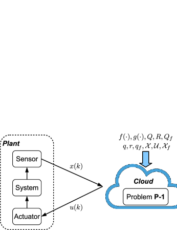
Figure 1: Cloud-based unsecure MPC architecture.

In a conventional MPC, the optimization problem (2) is solved at each time step based on the current state $x(k)$, and the first element of the optimal input sequence $\bm{U}^{*}_{k}=\begin{bmatrix}u_{0|k}^{*\top},\cdots,u_{N-1|k}^{*\top}\end{bmatrix}^{\top}$ is applied to the system, i.e., $u(k)=u_{0|k}^{*}$, and the system evolves one step. The process is then repeated. With gentle assumptions and by appropriately selecting the weighting matrix $Q_{f}$ and terminal set $\mathcal{X}_{f}$, the resulting closed-loop system can achieve guaranteed asymptotical stability [26].

The optimization problem in (2) is a nonlinear programming problem that requires significant computation power, which is very challenging to solve onboard considering limited onboard computation and stringent real-time constraints for many cyber-physical systems. This challenge is exacerbated when the dimension of the system state and the prediction horizon are large. To address this problem, cloud-based MPC is a viable framework where the complex computation is outsourced to the cloud that has superior computational power. The ultra low latency brought by 5G technologies makes this framework especially appealing. Specifically, the common cloud-based MPC architecture is shown in Fig. 1, which includes the following two phases:

• Handshaking Phase: The local plant sends $\left\{f(\cdot),g(\cdot),Q,R,Q_{f},\mathcal{X},\mathcal{U},\mathcal{X}_{f}\right\}$ to the cloud, that is, the necessary information for the cloud to set up the nonlinear programming problem in (2).

• Execution Phase: At each time step $k$, the plant first sends its state information $x(k)$ to the cloud. Then the cloud computes $u(k)$ by solving the optimization problem (2) and sends the resultant $u(k)$ to the plant. Finally, the plant applies $u(k)$ to the actuators and the system evolves one step.

II-B Attack Model

As described above, for the conventional cloud-based MPC, the local plant needs to provide the cloud with the system state, dynamic model, objective function, and constraints, which may contain confidential information that needs to be protected from an external eavesdropper or the untrusted cloud. In this paper, we consider the following two attack models:

• Eavesdropping attacks are attacks in which an external eavesdropper wiretaps communication channels to intercept exchanged messages in an attempt to learn the information about sending parties.

• Honest-but-curious attacks are attacks in which the untrusted cloud follows all protocol steps correctly but is curious and collects all received intermediate data in an attempt to learn the information about the local plant.

In particular, we consider the case that the privacy-sensitive information are contained in the system state $x(k)$ and input $u(k)$. It is clear that the attacker can successfully eavesdrop the messages $x(k)$ and $u(k)$ when the conventional cloud-based MPC architecture introduced in Section II-A is adopted. The objective of this paper is to develop a masking mechanism to modify the exchanged information between the local plant and the cloud such that an equivalent MPC problem is solved without affecting system performance while preventing the attacker from wiretapping the system state $x(k)$ and input $u(k)$.

III Main Results

In this section, we present our privacy-preserved cloud-based nonlinear MPC framework. We first show that by applying affine masking on the states and controls, and transforming the cost terms and system dynamics accordingly, the transformed nonlinear MPC problem solved on the cloud is equivalent to the original problem. We then show that this affine transformation can protect the privacy of the system states and inputs by virtue of indistinguishability.

III-A Affine masking and problem reformulation

Inspired by the works [19, 20, 7] that exploit linear transformations for linear MPCs, in this section, we design affine transformation maps to accomplish the privacy protection for the considered cloud-based nonlinear MPC. More precisely, two invertible affine maps $\iota_{x}(\cdot):=\left\{P_{x},t_{x}\right\}$ and $\iota_{u}(\cdot):=\left\{P_{u},t_{u}\right\}$ are introduced to transform the state $x(k)$ and input $u(k)$ to the new state $\bar{x}(k)$ and input $\bar{u}(k)$, as follows:

$$\bar{x}(k) =\iota_{x}(x(k))=P_{x}(x(k)+t_{x}),$$ (3)

$$\bar{u}(k) =\iota_{u}(u(k))=P_{u}(u(k)+t_{u}),$$

where $P_{x}\in\mathbb{R}^{n\times n}$, $P_{u}\in\mathbb{R}^{m\times m}$ are random invertible matrices, and $t_{x}\in\mathbb{R}^{n}$, $t_{u}\in\mathbb{R}^{m}$ are random non-zero vectors with compatible dimensions. From (1) and (3), it follows that the transformed system state evolves according to the following dynamics:

$$\bar{x}(k+1)=\bar{\Phi}(\bar{x}(k),\bar{u}(k))=\bar{f}(\bar{x}(k))+\bar{g}(\bar{x}(k))\bar{u}(k),$$ (4)

where $\bar{f}(\cdot)\in\mathbb{R}^{n}$ and $\bar{g}(\cdot)\in\mathbb{R}^{n\times m}$ are defined as

$$\bar{f}(\bar{x}(k)) =P_{x}\left(f\circ\iota_{x}^{-1}(\bar{x}(k))-g\circ\iota_{x}^{-1}(\bar{x}(k))t_{u}+t_{x}\right),$$ (5)

$$\bar{g}(\bar{x}(k)) =P_{x}g\circ\iota_{x}^{-1}(\bar{x}(k))P_{u}^{-1},$$

with $\circ$ denoting function composition. As will be shown below, the affine maps are able to mask the real system state $x(k)$ and input $u(k)$ to protect the privacy, and in the cloud a new optimization problem with respect to $\bar{x}(k)$, $\bar{u}(k)$, and the new system dynamics (4) are solved. Specifically, with the affine maps $\left\{P_{x},t_{x}\right\}$ and $\left\{P_{u},t_{u}\right\}$, one can show that P-1 can be transformed into the following problem:

$$\textbf{P-2}: \min_{\bar{\bm{U}}_{k}}\bar{J}_{N}(\bar{x}(k),\bar{\bm{U}}_{k})$$ (6)

$$=\sum_{i=0}^{N-1}(\bar{x}_{i|k}^{\top}\bar{Q}\bar{x}_{i|k}+\bar{q}^{\top}\bar{x}_{i|k}+\bar{u}_{i|k}^{\top}\bar{R}\bar{u}_{i|k}+\bar{r}^{\top}\bar{u}_{i|k})$$

$$\;\;\;\;+\bar{x}_{N|k}^{\top}\bar{Q}_{f}\bar{x}_{N|k}+\bar{q}_{f}^{\top}\bar{x}_{N|k},$$

s.t. $$\bar{x}_{i+1|k}=\bar{f}(\bar{x}_{i|k})+\bar{g}(\bar{x}_{i|k})\bar{u}_{i|k},i=0,\cdots,N-1,$$

$$\bar{x}_{i|k}\in\bar{\mathcal{X}},i=0,\cdots,N-1,$$

$$\bar{u}_{i|k}\in\bar{\mathcal{U}},i=0,\cdots,N-1,$$

$$\bar{x}_{N|k}\in\bar{\mathcal{X}}_{f},$$

$$\bar{x}_{0|k}=\bar{x}(k),\bar{\bm{U}}_{k}=\begin{bmatrix}\bar{u}_{0|k}^{\top},\cdots,\bar{u}_{N-1|k}^{\top}\end{bmatrix}^{\top},$$

where $\bar{Q}\in\mathbb{R}^{n\times n}$, $\bar{q}\in\mathbb{R}^{n}$, $\bar{R}\in\mathbb{R}^{m\times m}$, $\bar{r}\in\mathbb{R}^{m}$, $\bar{Q}_{f}\in\mathbb{R}^{n\times n}$, and $\bar{q}_{f}\in\mathbb{R}^{n}$ are defined as

$$\bar{Q} =P_{x}^{-\top}QP_{x}^{-1},\;\;\;\bar{q}=-2P_{x}^{-\top}Qt_{x},$$ (7)

$$\bar{R} =P_{u}^{-\top}RP_{u}^{-1},\;\;\;\bar{r}=-2P_{u}^{-\top}Rt_{u},$$

$$\bar{Q}_{f} =P_{x}^{-\top}Q_{f}P_{x}^{-1},\;\;\;\bar{q}_{f}=-2P_{x}^{-\top}Q_{f}t_{x}.$$

Moreover, in (6), $\bar{\mathcal{X}}$, $\bar{\mathcal{X}}_{f}$ and $\bar{\mathcal{U}}$ are the corresponding constraint sets of $\mathcal{X}$, $\mathcal{X}_{f}$ and $\mathcal{U}$ under the affine maps $\left\{P_{x},t_{x}\right\}$ and $\left\{P_{u},t_{u}\right\}$, respectively. This indicates that $\forall x\in\mathcal{X}$, $\iota_{x}(x)=P_{x}(x+t_{x})\in\bar{\mathcal{X}}$; vice versa $\forall\bar{x}\in\bar{\mathcal{X}}$, $\iota_{x}^{-1}(\bar{x})=P_{x}^{-1}\bar{x}-t_{x}\in\mathcal{X}$ (similarly for $\mathcal{X}_{f}$, $\bar{\mathcal{X}}_{f}$ and $\mathcal{U}$, $\bar{\mathcal{U}}$).

After introducing the affine maps, compared to the conventional cloud-based MPC in Section II-B, our privacy-preserved cloud-based nonlinear MPC architecture is modified as shown in Fig. 2:

• Handshaking Phase: Given the affine maps $\left\{P_{x},t_{x}\right\}$ and $\left\{P_{u},t_{u}\right\}$, the local plant transforms its system dynamics, objective function and constraint sets into $\left\{\bar{f}(\cdot),\bar{g}(\cdot),\bar{Q},\bar{q},\bar{R},\bar{r},\bar{Q}_{f},\bar{q}_{f},\bar{\mathcal{X}},\bar{\mathcal{U}},\bar{\mathcal{X}}_{f}\right\}$ and sends them to the cloud to provide necessary information for the cloud to set up the nonlinear programming problem (6).

• Execution Phase: At each time step $k$, the local plant first encodes $x(k)$ into $\bar{x}(k)$ with $\left\{P_{x},t_{x}\right\}$ and sends $\bar{x}(k)$ to the cloud. Then the cloud computes $\bar{u}(k)$ by solving the optimization problem (6) and sends the solution $\bar{u}(k)$ to the local plant. Finally, the plant uses $\left\{P_{u},t_{u}\right\}$ to decode $\bar{u}(k)$ (i.e., $u(k)=\iota_{u}^{-1}(\bar{u}(k))=P_{u}^{-1}\bar{u}(k)-t_{u}$) and then applies the resultant $u(k)$ to the actuators. The system then evolves one step.

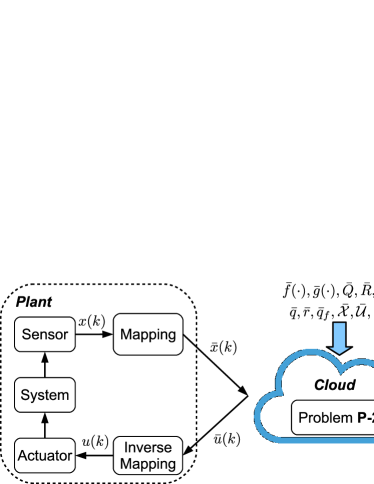
Figure 2: Cloud-based privacy-preservation MPC architecture with affine masking.

Note that under the privacy-preserved cloud-based MPC architecture, the exchanged information between the plant and the cloud during the execution phase is $\bar{x}(k)$ and $\bar{u}(k)$, instead of the actual system state $x(k)$ and input $u(k)$. In the sequel, we first show that the transformed MPC problem solved on the cloud is equivalent to the original MPC problem, and we then show that the privacy of $x(k)$ and $u(k)$ is protected.

Lemma 1.

Under the affine transformation mechanism, the optimization problem P-2 is equivalent to P-1, i.e., if $\bar{\bm{U}}^{*}_{k}=\begin{bmatrix}\bar{u}_{0|k}^{*\top},\cdots,\bar{u}_{N-1|k}^{*\top}\end{bmatrix}^{\top}$ is the solution to P-2, then the transformed control via inverse mapping $\bm{U}^{*}_{k}=\begin{bmatrix}u_{0|k}^{*\top},\cdots,u_{N-1|k}^{*\top}\end{bmatrix}^{\top}=\begin{bmatrix}(P_{u}^{-1}\bar{u}_{0|k}^{*}-t_{u})^{\top},\cdots,(P_{u}^{-1}\bar{u}_{N-1|k}^{*}-t_{u})^{\top}\end{bmatrix}^{\top}$ is the solution to P-1.

Proof:

With our designed state and control transformations in (3), the cost term transformations in (7), and the definitions of $J_{N}(\cdot,\cdot)$ and $\bar{J}_{N}(\cdot,\cdot)$, it can be shown that

$$J_{N}(x(k),\bm{U}_{k})=\bar{J}_{N}(\bar{x}(k),\bar{\bm{U}}_{k})+\varrho,$$ (8)

where $\varrho=\sum_{i=1}^{N-1}\left(t_{x}^{\top}Qt_{x}+t_{u}^{\top}Rt_{u}\right)+t_{x}^{\top}Q_{f}t_{x}\in\mathbb{R}$ is a constant. We now use proof by contradiction, that is, we assume that $\bar{\bm{U}}_{k}^{*}$ is the solution to problem P-2 but $\bm{U}_{k}^{*}$ is not the solution to problem P-1. This means that there exists an optimal sequence (other than $\bm{U}_{k}^{*}$) $\bm{U}_{k}^{**}=\begin{bmatrix}u_{0|k}^{**\top},\cdots,u_{N-1|k}^{**\top}\end{bmatrix}^{\top}$ such that

$$J_{N}(x(k),\bm{U}_{k}^{**})<J_{N}(x(k),\bm{U}_{k}^{*}).$$ (9)

Let $\bar{\bm{U}}_{k}^{**}=\begin{bmatrix}\bar{u}_{0|k}^{**\top},\cdots,\bar{u}_{N-1|k}^{**\top}\end{bmatrix}^{\top}=\begin{bmatrix}(P_{u}(u_{0|k}^{**}+t_{u}))^{\top},\cdots,(P_{u}(u_{N-1|k}^{**}+t_{u}))^{\top}\end{bmatrix}^{\top}$. According to (8), (9) can be rewritten as

$$\bar{J}_{N}(\bar{x}(k),\bar{\bm{U}}_{k}^{**})+\varrho<\bar{J}_{N}(\bar{x}(k),\bar{\bm{U}}_{k}^{*})+\varrho,$$ (10)

which contradicts the assumption that $\bar{\bm{U}}_{k}^{*}$ is the solution to problem P-2. The proof is complete. ∎

III-B Privacy Preservation

We next discuss the privacy notion used in this paper. As mentioned in the previous section, the attacker aims to infer the system state $x(k)$ and control input $u(k)$. Under the privacy-preserved cloud-based MPC architecture discussed above, the attacker will have access to $\bar{x}(k)$ and $\bar{u}(k)$ at each time step $k$, and we need to show that for any $\kappa\in\mathbb{N}_{+}$, $x_{[0,\kappa]}=\{x(0),\cdots,x(\kappa)\}$ and $u_{[0,\kappa]}=\{u(0),\cdots,u(\kappa)\}$ cannot be distinguished from $\bar{x}_{[0,\kappa]}=\{\bar{x}(0),\cdots,\bar{x}(\kappa)\}$ and $\bar{u}_{[0,\kappa]}=\{\bar{u}(0),\cdots,\bar{u}(\kappa)\}$. To facilitate the following development, two triples $\Omega$ and $\bar{\Omega}$ are defined as

$$\Omega =\left\{\left\{f(\cdot),g(\cdot)\right\},J_{N}(\cdot,\cdot),\left\{\mathcal{X},\mathcal{U},\mathcal{X}_{f}\right\}\right\},$$ (11)

$$\bar{\Omega} =\left\{\left\{\bar{f}(\cdot),\bar{g}(\cdot)\right\},\bar{J}_{N}(\cdot,\cdot),\left\{\bar{\mathcal{X}},\bar{\mathcal{U}},\bar{\mathcal{X}}_{f}\right\}\right\}.$$

It can be seen that the triples $\Omega$ and $\bar{\Omega}$ can be used to define the optimization problem in (2) and (6), respectively. We call $\left\{x_{[0,\kappa]},u_{[0,\kappa]}\right\}$ a solution to the optimization problem (2) defined by $\Omega$ if $\left\{x_{[0,\kappa]},u_{[0,\kappa]}\right\}$ is a trajectory of the nonlinear system $\left\{f(\cdot),g(\cdot)\right\}$ minimizing objective function $J_{N}(\cdot,\cdot)$ under constraints described by $\left\{\mathcal{X},\mathcal{U},\mathcal{X}_{f}\right\}$. Moreover, we use $\Omega\xRightarrow{\{P_{x},t_{x},P_{u},t_{u}\}}\bar{\Omega}$ to denote that $\bar{\Omega}$ is the transformed triple of $\Omega$ under the affine maps $\left\{P_{x},t_{x}\right\}$ and $\left\{P_{u},t_{u}\right\}$.

Given $\bar{\Omega}$, for any feasible input sequence $\bar{x}_{[0,\kappa]}$ and output sequence $\bar{u}_{[0,\kappa]}$ received by the attacker, the set $\Delta_{\bar{\Omega}}(\bar{x}_{[0,\kappa]},\bar{u}_{[0,\kappa]})$ is defined as

$$\Delta_{\bar{\Omega}}(\bar{x}_{[0,\kappa]},\bar{u}_{[0,\kappa]})=\{x_{[0,\kappa]},u_{[0,\kappa]}:\exists\{P_{x},t_{x},P_{u},t_{u}\}\;\text{and}\;\Omega$$ (12)

$$\text{s.t.}\;\bar{x}(k)=P_{x}(x(k)+t_{x}),\bar{u}(k)=P_{u}(u(k)+t_{u}),$$

$$\Omega\xRightarrow{\{P_{x},t_{x},P_{u},t_{u}\}}\bar{\Omega},\text{and}\left\{x_{[0,\kappa]},u_{[0,\kappa]}\right\}\text{is the solution to}\;\Omega\}.$$

Essentially, the set $\Delta_{\bar{\Omega}}(\bar{x}_{[0,\kappa]},\bar{u}_{[0,\kappa]})$ includes all possible valuations of $\{x_{[0,\kappa]},u_{[0,\kappa]}\}$ that can be transformed into $\{\bar{x}_{[0,\kappa]},\bar{u}_{[0,\kappa]}\}$ with corresponding affine maps $\{P_{x},t_{x},P_{u},t_{u}\}$. The diameter of $\Delta_{\bar{\Omega}}(\bar{x}_{[0,\kappa]},\bar{u}_{[0,\kappa]})$, a metric that measures the distance (dissimilarity) between its elements, is defined as

$$\text{Diam}_{\Delta_{\bar{\Omega}}}(\bar{x}_{[0,\kappa]},\bar{u}_{[0,\kappa]})=\sup_{w,w^{\prime}\in\Delta_{\bar{\Omega}}(\bar{x}_{[0,\kappa]},\bar{u}_{[0,\kappa]})}\left|w-w^{\prime}\right|_{\min},$$ (13)

where $\left|w-w^{\prime}\right|_{\min}=\min_{l\in\left\{1,\cdots,(n+m)(\kappa+1)\right\}}\left|w_{l}-w^{\prime}_{l}\right|$ with $w_{l}$ and $w^{\prime}_{l}$ being the $l$-th element of $w$ and $w^{\prime}$, respectively.

Definition 1 ($\infty$-Diversity with Unbounded Diameter).

The privacy of the actual system state $x_{[0,\kappa]}$ and input $u_{[0,\kappa]}$ is preserved if $\left.1\right)$ the cardinality of the set $\Delta_{\bar{\Omega}}(\bar{x}_{[0,\kappa]},\bar{u}_{[0,\kappa]})$ is infinite, and $\left.2\right)$ $\text{Diam}_{\Delta_{\bar{\Omega}}}(\bar{x}_{[0,\kappa]},\bar{u}_{[0,\kappa]})=\infty$.

In the $\infty$-Diversity with Unbounded Diameter privacy defined above, the first condition requires that there are infinite sets of $\{x_{[0,\kappa]},u_{[0,\kappa]}\}$, $\{P_{x},t_{x},P_{u},t_{u}\}$ and $\Omega$ that can generate the same $\{\bar{x}_{[0,\kappa]},\bar{u}_{[0,\kappa]}\}$ received by the attacker. As a result, it is impossible for the attacker to use $\{\bar{x}_{[0,\kappa]},\bar{u}_{[0,\kappa]}\}$ to infer the actual system state and input information. Moreover, the second condition requires that the difference between the possible valuations of $\{x_{[0,\kappa]},u_{[0,\kappa]}\}$ could be arbitrarily large, which makes the attacker cannot even approximately estimate (e.g., find a finite range for) the private signals.

The definition is an extension to the $l$-diversity [27] which has been widely adopted in formal privacy analysis on attribute privacy of tabular datasets and has recently been extended to define privacy in linear dynamic networks [28]. Essentially, $l$-diversity requires that there are at least $l$ different possible values for the privacy sensitive data attributes, and a greater $l$ indicates greater indistinguishability. In our work, Definition 1 requires that there exist infinite sets of states/inputs and linear transformation combinations that can generate the same accessible information to the adversary. In addition, we require and the difference of the states/inputs in these sets can be arbitrarily large. This makes the adversary unable to find a unique value or even estimate a rough range of the private parameters.

Remark 1.

Compared to differential privacy that injects independent noises to obfuscate private values that will inevitably compromise algorithmic accuracy [29, 30], the considered privacy definition with the affine masking scheme does not affect system performance as the transformed problem is equivalent to the original one as shown in Section III-A. Mutual information-based privacy preservation relies on explicit statistical models of source data and side information [31] which, however, is not generally available in the considered cloud-based MPC problem. Semantic security requires “nothing is learned” by the adversary from its accessible data, which intrinsically inhibits any meaningful data utility and can resist arbitrary side information [29, 28]. In our problem, the eavesdropper has access to all exchanged information that is necessary for the cloud to perform the optimizations. Therefore, semantic security is too restrictive and not applicable to our problem.

We now show that the affine transformation mechanism can achieve privacy preservation based on Definition 1.

Theorem 1.

Under the affine masking mechanism described in Section III-A, the system states and control inputs are $\infty$-diversity-with-unbounded-diameter private, that is, the attacker cannot infer the actual system state $x(k)$ and input $u(k)$ with any guaranteed accuracy.

Proof:

We prove Theorem 1 by proving the two conditions in Definition 1. We first show that under the affine masking scheme, the cardinality of the set $\Delta(\bar{x}_{[0,\kappa]},\bar{u}_{[0,\kappa]})$ is infinite. Specifically, given the sequence $\{\bar{x}_{[0,\kappa]},\bar{u}_{[0,\kappa]}\}$ and $\bar{\Omega}$ accessible to the attacker, for an arbitrary affine map $\{P_{x}^{\prime},t_{x}^{\prime},P_{u}^{\prime},t_{u}^{\prime}\}$ such that $P_{x}^{\prime}$ and $P_{u}^{\prime}$ are invertible, a sequence $\{x^{\prime}_{[0,\kappa]},u^{\prime}_{[0,\kappa]}\}$ and $\Omega^{\prime}$ can be uniquely determined based on $\{\bar{x}_{[0,\kappa]},\bar{u}_{[0,\kappa]}\}$ and $\bar{\Omega}$ by using $\{P_{x}^{\prime},t_{x}^{\prime},P_{u}^{\prime},t_{u}^{\prime}\}$ as an inverse mapping. As there exists infinitely many such affine maps $\{P_{x}^{\prime},t_{x}^{\prime},P_{u}^{\prime},t_{u}^{\prime}\}$, there exists infinitely many $\{x^{\prime}_{[0,\kappa]},u^{\prime}_{[0,\kappa]}\}$ such that via proper affine transformations, the attacker will receive the same accessed information: $\{\bar{x}_{[0,\kappa]},\bar{u}_{[0,\kappa]}\}$ and $\bar{\Omega}$, which thus satisfies the first condition in Definition 1.

We now prove the second condition in Definition 1. For any $w,w^{\prime}\in\Delta_{\bar{\Omega}}(\bar{x}_{[0,\kappa]},\bar{u}_{[0,\kappa]})$ (i.e., $\{x_{[0,\kappa]},u_{[0,\kappa]}\},\{x^{\prime}_{[0,\kappa]},u^{\prime}_{[0,\kappa]}\}\in\Delta_{\bar{\Omega}}(\bar{x}_{[0,\kappa]},\bar{u}_{[0,\kappa]})$) with $\{P_{x},t_{x},P_{u},t_{u}\}$ and $\{P_{x}^{\prime},t_{x}^{\prime},P_{u}^{\prime},t_{u}^{\prime}\}$ being the corresponding affine maps, we have $\bar{x}(k)=P_{x}(x(k)+t_{x})=P_{x}^{\prime}(x^{\prime}(k)+t^{\prime}_{x})$ and $\bar{u}(k)=P_{u}(u(k)+t_{u})=P_{u}^{\prime}(u^{\prime}(k)+t^{\prime}_{u})$, which indicates that

$$x(k)=P_{x}^{-1}\bar{x}(k)-t_{x},\;\;x^{\prime}(k)=(P_{x}^{\prime})^{-1}\bar{x}(k)-t^{\prime}_{x},$$ (14)

$$u(k)=P_{u}^{-1}\bar{u}(k)-t_{u},\;\;u^{\prime}(k)=(P_{u}^{\prime})^{-1}\bar{u}(k)-t^{\prime}_{u}.$$

Based on (14), it can be obtained that

$$\left|w-w^{\prime}\right|_{\min}=\left|\begin{matrix}(P_{x}^{-1}-(P_{x}^{\prime})^{-1})\bar{x}(0)-(t_{x}-t_{x}^{\prime})\\ \vdots\\ (P_{x}^{-1}-(P_{x}^{\prime})^{-1})\bar{x}(\kappa)-(t_{x}-t_{x}^{\prime})\\ (P_{u}^{-1}-(P_{u}^{\prime})^{-1})\bar{u}(0)-(t_{u}-t_{u}^{\prime})\\ \vdots\\ (P_{u}^{-1}-(P_{u}^{\prime})^{-1})\bar{u}(\kappa)-(t_{u}-t_{u}^{\prime})\end{matrix}\right|_{\min}$$ (15)

$$=\left|\begin{matrix}(I_{\kappa+1}\otimes(P_{x}^{-1}-(P_{x}^{\prime})^{-1}))\bar{x}_{[0,\kappa]}-1_{\kappa+1}\otimes(t_{x}-t_{x}^{\prime})\\ (I_{\kappa+1}\otimes(P_{u}^{-1}-(P_{u}^{\prime})^{-1}))\bar{u}_{[0,\kappa]}-1_{\kappa+1}\otimes(t_{u}-t_{u}^{\prime})\end{matrix}\right|_{\min}$$

$$\geq\left|\begin{matrix}1_{\kappa+1}\otimes(t_{x}-t_{x}^{\prime})\\ 1_{\kappa+1}\otimes(t_{u}-t_{u}^{\prime})\end{matrix}\right|_{\min}-\left|\begin{matrix}(I_{\kappa+1}\otimes(P_{x}^{-1}-(P_{x}^{\prime})^{-1}))\bar{x}_{[0,\kappa]}\\ (I_{\kappa+1}\otimes(P_{u}^{-1}-(P_{u}^{\prime})^{-1}))\bar{u}_{[0,\kappa]}\end{matrix}\right|_{\max},$$

where $\otimes$ is the Kronecker product, $I_{\kappa+1}\in\mathbb{R}^{(\kappa+1)\times(\kappa+1)}$ is the identity matrix, and $1_{\kappa+1}\in\mathbb{R}^{\kappa+1}$ is the column vector with all the entries being ones. Furthermore, by using (13) and (15), the diameter of the set $\Delta_{\bar{\Omega}}(\bar{x}_{[0,\kappa]},\bar{u}_{[0,\kappa]})$ can be derived as follows:

$$\text{Diam}_{\Delta_{\bar{\Omega}}}(\bar{x}_{[0,\kappa]},\bar{u}_{[0,\kappa]})=\sup_{w,w^{\prime}\in\Delta_{\bar{\Omega}}(\bar{x}_{[0,\kappa]},\bar{u}_{[0,\kappa]})}\left|w-w^{\prime}\right|_{\min}$$ (16)

$$\geq\sup_{t_{x},t_{x}^{\prime}\in\mathbb{R}^{n},t_{u},t_{u}^{\prime}\in\mathbb{R}^{m}}\left|\begin{matrix}1_{\kappa+1}\otimes(t_{x}-t_{x}^{\prime})\\ 1_{\kappa+1}\otimes(t_{u}-t_{u}^{\prime})\end{matrix}\right|_{\min}$$

$$\;\;\;\;-\inf_{P_{x},P_{x}^{\prime}\in\mathbb{R}^{n\times n},P_{u},P_{u}^{\prime}\in\mathbb{R}^{m\times m}}\left|\begin{matrix}(I_{\kappa+1}\otimes(P_{x}^{-1}-(P_{x}^{\prime})^{-1}))\bar{x}_{[0,\kappa]}\\ (I_{\kappa+1}\otimes(P_{u}^{-1}-(P_{u}^{\prime})^{-1}))\bar{u}_{[0,\kappa]}\end{matrix}\right|_{\max}$$

$$=\infty.$$

Thus, the second condition in Definition 1 is satisfied. ∎

Remark 2.

The proposed approach is quite different from the existing algebraic transformation methods for linear systems [19, 20, 7]. The scheme proposed in [19] only works for special objective functions and linear input constraints, and neither state nor input constraints are well considered in [20]. Our developed approach can be applied to more general MPC problems as we consider nonlinear systems, objective function described by general quadratic form, and state and input constraints. Different from the work [7] that quantifies the privacy via the dimension of the manifold that describes the uncertainty experienced by the adversary, we use the set cardinality and diameter to define the privacy notion for cloud-based nonlinear MPC. Note that the set dimension based privacy quantification in [7] is derived based on the characteristics of linear systems, which cannot be applied to nonlinear systems.

IV Extension to Output-feedback MPC

The aforementioned cloud-based MPC methods require that all system states are measurable to perform the state-feedback control. However, for some systems, not all states are accessible but an output vector is available for output feedback control designs. Therefore, in this section we extend the privacy-preserved cloud-based MPC design to the output-feedback case. Specifically, let $y(k)\in\mathbb{R}^{p}$ be the system output described by

$$y(k)=Cx(k),$$ (17)

where $C\in\mathbb{R}^{p\times n}$. We assume that the system is observable and the state $x(k)$ can be estimated via a high-gain observer [32] in the following form:

$$\hat{x}(k+1)=\Phi(\hat{x}(k),u(k))+H(y(k)-C\hat{x}(k)),$$ (18)

where $\hat{x}(k)\in\mathbb{R}^{n}$ is the estimate of $x(k)$ and $H\in\mathbb{R}^{n\times p}$ is the gain matrix. The estimated state $\hat{x}(k)$ is then fed into the MPC problem (2) to obtain the solutions. Under the output-feedback case, the conventional cloud-based MPC is typically implemented as follows:

• Handshaking Phase: The local plant sends $\left\{f(\cdot),g(\cdot),Q,R,Q_{f},\mathcal{X},\mathcal{U},\mathcal{X}_{f},H,C\right\}$ to the cloud, which are necessary information for the cloud to perform state estimation and subsequent MPC based on the estimated state.

• Execution Phase: At each time step $k$, the plant first sends $y(k)$ to the cloud. Then the cloud estimates the system state $\hat{x}_{k}$ via (18), computes $u(k)$ based on $\hat{x}_{k}$ by solving the optimization problem shown in (2) and sends $u(k)$ to the plant. Finally, the plant applies $u(k)$ to the actuators and the system evolves one step.

The objective now is to avoid leaking the privacy-sensitive information $y(k)$, $\hat{x}(k)$, and $u(k)$ to the attacker. Similar to (3), an invertible affine map is introduced to mask $y(k)$ as follows:

$$\bar{y}(k)=\iota_{y}(y(k))=P_{y}(y(k)+t_{y}),$$ (19)

where $P_{y}\in\mathbb{R}^{p\times p}$ is an invertible matrix and $t_{y}\in\mathbb{R}^{p}$ is an offset vector. According to (3), (17) and $\eqref{equ_affine_y}$, it can be obtained that

$$\bar{y}(k)=\bar{C}\bar{x}(k)+\bar{\sigma}_{y},$$ (20)

with $\bar{C}\in\mathbb{R}^{p\times n}$ and $\bar{\sigma}_{y}\in\mathbb{R}^{p}$ being defined as

$$\bar{C} =P_{y}CP_{x}^{-1},$$ (21)

$$\bar{\sigma}_{y} =P_{y}(-Ct_{x}+t_{y}).$$

Moreover, from (4), (18) and (20), it can be shown that $\bar{x}(k)$ can be estimated with $\bar{y}(k)$ via the following observer:

$$\hat{\bar{x}}(k+1)=\bar{\Phi}(\hat{\bar{x}}(k),\bar{u}(k))+\bar{H}(\bar{y}(k)-\bar{C}\hat{\bar{x}}(k)-\bar{\sigma}_{y}),$$ (22)

where $\bar{H}\in\mathbb{R}^{n\times p}$ is given by

$$\bar{H}=P_{x}HP_{y}^{-1}.$$ (23)

The cloud-based privacy-preserved MPC under the output-feedback setup can then be performed with the following modified procedures:

• Handshaking Phase: Given the affine maps $\left\{P_{x},t_{x}\right\}$, $\left\{P_{u},t_{u}\right\}$ and $\left\{P_{y},t_{y}\right\}$, the plant transforms its system dynamics, objective function, constraint sets and observer into $\left\{\bar{f}(\cdot),\bar{g}(\cdot)\right\}$, $\bar{J}_{N}(\cdot,\cdot)$ (i.e., $\left\{\bar{Q},\bar{q},\bar{R},\bar{r},\bar{Q}_{f},\bar{q}_{f}\right\}$), $\left\{\bar{\mathcal{X}},\bar{\mathcal{U}},\bar{\mathcal{X}}_{f}\right\}$ and $\left\{\bar{H},\bar{C},\bar{\sigma}_{y}\right\}$ and sends them to the cloud.

• Execution Phase: At each time step $k$, the plant first encodes $y(k)$ into $\bar{y}(k)=P_{y}(y(k)+t_{y})$ and sends $\bar{y}(k)$ to the cloud. Then the cloud estimates the system state via (22), computes $\bar{u}(k)$ by solving the optimization problem (6) and sends $\bar{u}(k)$ to the plant. Finally, the plant uses $\left\{P_{u},t_{u}\right\}$ to decode $\bar{u}(k)$ (i.e., $u(k)=\iota_{u}^{-1}(\bar{u}(k))=P_{u}^{-1}\bar{u}(k)-t_{u}$) and then applies $u(k)$ to the actuators. The system evolves one step.

Theorem 2.

Under the affine masking mechanism described in this subsection, the system outputs, states and control inputs are $\infty$-diversity-with-unbounded-diameter private, that is, the attacker cannot infer the actual outputs $y(k)$, system state $x(k)$ and input $u(k)$ with any guaranteed accuracy.

Proof:

The proof follows similar arguments in Theorem 1. ∎

V Simulation Results

In this section, we perform numerical simulations to demonstrate the efficacy of the developed approach. As shown in Fig. 3, we consider the inverted pendulum mounted to a cart problem, which has the continuous-time model given by [33]:

$$\ddot{z} =\frac{F-K_{d}\dot{z}-m_{pend}L\dot{\theta}^{2}\sin(\theta)+m_{pend}g\sin(\theta)\cos(\theta)}{m_{cart}+m_{pend}\sin^{2}(\theta)},$$ (24)

$$\ddot{\theta} =\frac{\ddot{z}\cos(\theta)+g\sin(\theta)}{L},$$

where $z$ is the cart position, $\theta$ is the pendulum angle, $m_{cart}=1$ kg is the cart mass, $m_{pend}=1$ kg is the pendulum mass, $L=0.5$ m is the length of the pendulum, $K_{d}=10$ Ns/m is the damping parameter, $g=9.81$ m/s² is the gravity acceleration, and $F$ is the variable force. The system state, input and output are defined as $x=\begin{bmatrix}z&\dot{z}&\theta&\dot{\theta}\end{bmatrix}^{\top}$, $u=F$ and $y=\begin{bmatrix}z&\theta\end{bmatrix}^{\top}$, respectively. We discretize the continuous-time model (24) with a sampling time of $\Delta T=0.1$ s. The control objective is to regulate the plant to the equilibrium $\begin{bmatrix}z&\dot{z}&\theta&\dot{\theta}\end{bmatrix}^{\top}=\begin{bmatrix}0&0&0&0\end{bmatrix}^{\top}$ by using the cloud-based MPC schemes. For the MPC formulation, the weighting matrices are selected as $Q=Q_{f}=\text{diag}\left(\begin{matrix}300&0.01&300&0.01\end{matrix}\right)$ and $R=1$, and the system state and input are subjected to the following constraints:

$$-10\leq x_{1}\leq 10,\;\;\;-100\leq u\leq 100.$$

Moreover, the affine maps $\left\{P_{x},t_{x}\right\}$, $\left\{P_{u},t_{u}\right\}$ and $\left\{P_{y},t_{y}\right\}$ are chosen as

$$P_{x} =\begin{bmatrix}-3&1.5&0&0\\ -1&-2&0&0\\ 0&0&2&-0.5\\ 0&0&-0.8&2\end{bmatrix},\;\;\;t_{x}=\begin{bmatrix}2\\ -3\\ 1\\ -1.5\end{bmatrix},$$

$$P_{u} =-2,\;\;\;t_{u}=5,$$

$$P_{y} =\begin{bmatrix}1.5&-0.4\\ -0.3&1.6\end{bmatrix},\;\;\;t_{y}=\begin{bmatrix}3\\ -4\end{bmatrix}.$$

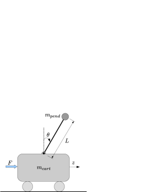
Figure 3: Inverted pendulum on a cart.

We first evaluate the unsecure (i.e., conventional) and secure (i.e., privacy-preserved) MPC schemes with state feedback. The simulation results are presented in Figs. 4 and 5. It can be found from Figs. 4 and 5 that the state and input trajectories obtained from the secure MPC is identical to the ones obtained by the unsecure MPC, and thus further demonstrates that the affine transformation mechanism can retain the control performance as the conventional unsecure MPC. Meanwhile as shown in Figs. 4 and 5, under the secure MPC, the state and input information collected by the cloud is quite different from the actual one, which makes the cloud unable to infer $x(k)$ and $u(k)$.

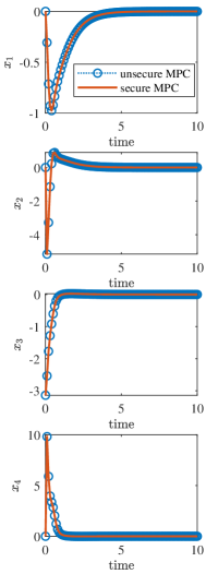
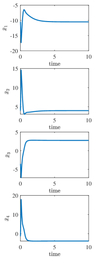
Figure 4: Simulation results with state-feedback MPC: (a) system state evolution in the plant under unsecure and secure MPC schemes, (b) state evolution in the cloud under secure MPC.

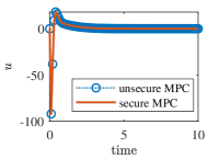
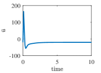
Figure 5: Simulation results with state-feedback MPC: (a) system input evolution in the plant under unsecure and secure MPC schemes, (b) input evolution in the cloud under secure MPC.

Furthermore, the cloud-based MPC schemes with output feedback are also applied to control the inverted pendulum system, where we use $z$ and $\theta$ as the measurements (i.e., $C=\begin{bmatrix}1&0&0&0\\ 0&0&1&0\end{bmatrix}$). The simulation results are shown in Figs. 6 and 7, from which it can be concluded that under the output-feedback case, the secure MPC scheme still can achieve the same control performance as the conventional method, while protecting the private state and input signals from being inferred by the cloud.

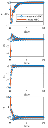
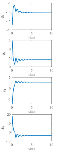
Figure 6: Simulation results with output-feedback MPC: (a) system state evolution in the plant under unsecure and secure MPC schemes, (b) state evolution in the cloud under secure MPC.

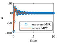
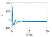
Figure 7: Simulation results with output-feedback MPC: (a) system input evolution in the plant under unsecure and secure MPC schemes, (b) input evolution in the cloud under secure MPC.

VI Conclusion

This paper developed an affine masking based privacy-preserved cloud-based nonlinear MPC framework. We considered eavesdropper and honest-but-curious adversaries who intend to infer the local plant’s system state and input and the $\infty$-diversity with unbounded diameter privacy notion was adopted. A simple yet effective affine transformation mechanism was designed to enable privacy preservation without affecting the MPC calculation. Furthermore, the proposed method was successfully extended to output-feedback MPC. Simulation results showed that by using the proposed method, the MPC problem can be addressed without disclosing private information to the cloud. Future work will include the extension of this framework to systems with uncertainties (e.g., robust and stochastic MPCs).

References

- [1] D. Q. Mayne, “Model predictive control: Recent developments and future promise,” Automatica, vol. 50, pp. 2967–2986, 2014.
- [2] N. Li, A. Girard, and I. Kolmanovsky, “Stochastic predictive control for partially observable markov decision processes with time-joint chance constraints and application to autonomous vehicle control,” Journal of Dynamic Systems, Measurement, and Control, vol. 141, no. 7, p. 071007, 2019.
- [3] M. Allenspach and G. J. J. Ducard, “Nonlinear model predictive control and guidance for a propeller-tilting hybrid unmanned air vehicle,” Automatica, vol. 132, p. 109790, 2021.
- [4] M. Liu, Y. Shi, and X. Liu, “Distributed MPC of aggregated heterogeneous thermostatically controlled loads in smart grid,” IEEE Transactions on Industrial Electronics, vol. 63, no. 2, pp. 1120–1129, 2016.
- [5] N. Li, K. Zhang, Z. Li, V. Srivastava, and X. Yin, “Cloud-assisted nonlinear model predictive control for finite-duration tasks,” arXiv preprint arXiv:2106.10604, 2021.
- [6] N. Schlüter and M. S. Darup, “Encrypted explicit MPC based on two-party computation and convex controller decomposition,” in Proceedings of the IEEE Conference on Decision and Control, 2020, pp. 5469–5476.
- [7] A. Sultangazin and P. Tabuada, “Symmetries and isomorphisms for privacy in control over the cloud,” IEEE Transactions on Automatic Control, vol. 66, no. 2, pp. 538–549, 2021.
- [8] R. L. Grossman, “The case for cloud computing,” IT Professional, vol. 11, no. 2, pp. 23–27, 2009.
- [9] Z. Li, I. Kolmanovsky, E. Atkins, J. Lu, D. Filev, and J. Michelini, “Cloud aided semi-active suspension control,” in Proceeding of the IEEE Symposium on Computational Intelligence in Vehicles and Transportation Systems, 2014, pp. 76–83.
- [10] Z. Li, I. V. Kolmanovsky, E. M. Atkins, J. Lu, D. P. Filev, and Y. Bai, “Road disturbance estimation and cloud-aided comfort-based route planning,” IEEE Transactions on Cybernetics, vol. 47, no. 11, pp. 3879–3891, 2017.
- [11] Z. Li, I. Kolmanovsky, E. Atkins, J. Lu, D. P. Filev, and J. Michelini, “Road risk modeling and cloud-aided safety-based route planning,” IEEE Transactions on Cybernetics, vol. 46, no. 11, pp. 2473–2483, 2016.
- [12] E. Ozatay, S. Onori, J. Wollaeger, U. Ozguner, G. Rizzoni, D. Filev, J. Michelini, and S. D. Cairano, “Cloud-based velocity profile optimization for everyday driving: A dynamic-programming-based solution,” IEEE Transactions on Intelligent Transportation Systems, vol. 15, no. 6, pp. 2491–2505, Dec 2014.
- [13] J. Petit and S. E. Shladover, “Potential cyberattacks on automated vehicles,” IEEE Transactions on Intelligent Transportation Systems, vol. 16, no. 2, pp. 546–556, 2015.
- [14] A. Munteanu, R. Muradore, M. Merro, and P. Fiorini, “On cyber-physical attacks in bilateral teleoperation systems: An experimental analysis,” in Proceedings of the IEEE Industrial Cyber-Physical Systems, 2018, pp. 159–166.
- [15] Y. Xu, G. Deng, T. Zhang, H. Qiu, and Y. Bao, “Novel denial-of-service attacks against cloud-based multi-robot systems,” Information Sciences, vol. 576, pp. 329–344, 2021.
- [16] M. S. Darup, A. Redder, I. Shames, F. Farokhi, and D. E. Quevedo, “Towards encrypted MPC for linear constrained systems,” IEEE Control Systems Letters, vol. 2, no. 2, pp. 195–200, 2018.
- [17] A. B. Alexandru, M. Morari, and G. J. Pappas, “Cloud-based MPC with encrypted data,” in Proceedings of the IEEE Conference on Decision and Control, 2018, pp. 5014–5019.
- [18] M. S. Darup, A. Redder, and D. E. Quevedo, “Encrypted cloud-based MPC for linear systems with input constraints,” IFAC-PapersOnLine, vol. 51, no. 20, pp. 535–542, 2018.
- [19] Z. Xu and Q. Zhu, “Secure and resilient control design for cloud enabled networked control systems,” in Proceedings of the first ACM workshop on cyber-physical systems-security and/or privacy, 2015, pp. 31–42.
- [20] ——, “Secure and practical output feedback control for cloud-enabled cyber-physical systems,” in Proceedings of the IEEE Conference on Communications and Network Security, 2017, pp. 416–420.
- [21] P. C. Weeraddana, G. Athanasiou, C. Fischione, and J. S. Baras, “Per-se privacy preserving solution methods based on optimization,” in Proceedings of the IEEE Conference on Decision and Control, 2013, pp. 206–211.
- [22] P. C. Weeraddana and C. Fischione, “On the privacy of optimization,” IFAC-PapersOnLine, vol. 50, no. 1, pp. 9502–9508, 2017.
- [23] O. L. Mangasarian, “Privacy-preserving linear programming,” Optimization Letters, vol. 5, no. 1, pp. 165–172, 2011.
- [24] C. Wang, K. Ren, and J. Wang, “Secure and practical outsourcing of linear programming in cloud computing,” in Proceedings of IEEE INFOCOM, 2011, pp. 820–828.
- [25] A. Bemporad, D. Bernardini, R. Long, and J. Verdejo, “Model predictive control of turbocharged gasoline engines for mass production,” in SAE Technical Paper. SAE International, 04 2018. [Online]. Available: https://doi.org/10.4271/2018-01-0875
- [26] J. B. Rawlings, D. Q. Mayne, and M. Diehl, Model Predictive Control: Theory, Computation, and Design. Nob Hill Publishing, 2017.
- [27] A. Machanavajjhala, D. Kifer, J. Gehrke, and M. Venkitasubramaniam, “l-diversity: Privacy beyond k-anonymity,” ACM Transactions on Knowledge Discovery from Data, vol. 1, no. 1, pp. 3–14, Mar. 2007.
- [28] Y. Lu and M. Zhu, “On privacy preserving data release of linear dynamic networks,” Automatica, vol. 115, p. 108839, May 2020.
- [29] C. Dwork and A. Roth, “The algorithmic foundations of differential privacy,” Foundations and Trends in Theoretical Computer Science, vol. 9, no. 3-4, pp. 211–407, 2014.
- [30] Z. Huang, S. Mitra, and G. Dullerud, “Differentially private iterative synchronous consensus,” in Proceedings of the ACM Workshop on Privacy in the Electronic Society, New York, NY, USA, 2012, pp. 81–90.
- [31] L. Sankar, S. R. Rajagopalan, and H. V. Poor, “Utility-privacy tradeoffs in databases: An information-theoretic approach,” IEEE Transactions on Information Forensics and Security, vol. 8, no. 6, pp. 838–852, Mar. 2013.
- [32] H. K. Khalil, Nonlinear Systems. Upper Saddle River, NJ: Prentice-Hall, 2002.
- [33] R. Gurumoorthy and S. Sanders, “Controlling non-minimum phase nonlinear systems–The inverted pendulum on a cart example,” in Proceedings of the American Control Conference, 1993, pp. 680–685.