Homogenization of a non-linear strongly coupled model of magnetorheological fluids

Abstract

This paper concerns the rigorous periodic homogenization for a non-linear strongly coupled system, which models a suspension of magnetizable rigid particles in a non-conducting carrier viscous Newtonian fluid. The fluid drags the particles, thus alters the magnetic field. Vice versa, the magnetic field acts on the particles, which in turn affect the fluid via the no-slip boundary condition. As the size of the particles approaches zero, it is shown that the suspension’s behavior is governed by a generalized magnetohydrodynamic system, where the fluid is modeled by a stationary Navier-Stokes system, while the magnetic field is modeled by Maxwell equations. A corrector result from the theory of two-scale convergence allows us to obtain the limit of the product of several weakly convergent sequences, where the div-curl lemma, which is a typical tool in these types of problems, is not applicable.

35B27, 74E30, 74F10, 76M50, 78M40.

1 Introduction

This paper is a counterpart of our previous works [16, 15], where we carried out the rigorous periodic homogenization of a weakly (one-way) coupled non-linear system modeling a non-dilute suspension of magnetizable particles in a viscous Newtonian fluid. In [16, 15], the fluid is assumed to be described by the stationary Stokes flow, and the particles are either paramagnetic or diamagnetic. The one-way coupling is understood as follows: the magnetic field alters the movement of the magnetizable particles, then the particles affect the fluid flow via a no-slip boundary assumption; however, the reverse effect is assumed to be negligible. For details and information about the manifestations of the one-way coupling (as well as of the full coupling), its applications, and further literature on the subject, we refer the reader to [16, 15] and references cited therein. In this paper, the full (two-way) coupling is considered, i.e. we also take into account the reverse effect: the fluid flow pushes the particles, thus generates an induced magnetic field that acts back on the original one. The mathematical formulation of the fully coupled model of the magnetic non-dilute suspension is given in Section 2 below.

Starting with the seminal work of Einstein on the effective viscosity of a suspension [23], there have been numerous studies on this subject, ranging from formal asymptotic analysis such as [43, 44, 42] to rigorous analysis, e.g. [48, 17, 32, 40, 45, 28, 20, 41, 37, 22, 19, 21, 7, 8] and references cited therein. The coupling between the velocity and the magnetic fields distinguishes our paper from the previously cited. In this paper, we propose a non-linear system to model the two-way coupling in the magnetorheological fluid, and derive, and rigorously justify, the corresponding effective system.

To overview the literature on this topic, we start with the phenomenological models proposed in e.g. [46, 52, 24, 50, 33], whose well-posedness were studied in e.g. [51, 34, 27, 6, 53]. A coupling mechanism, similar to the one discussed in this paper, was also considered in [49], where a different model describing fluids was used. The authors in [49] though obtained the results using formal asymptotic analysis. Although similar models in different contexts were also studied in [56, 25], to the best of our knowledge, this paper is the first one to deal with the fully-coupled model for magnetorheological fluids using the rigorous homogenization approach. Lastly, we mention that the rigorous homogenization for the system described by one-way fluid-particle coupling was solved in [16, 15] with a fairly general assumption on the smoothness of the coefficients.

In what follows below, after a non-linear model for the magnetorheological fluid is established, we obtain the well-posedness and a priori estimates for its solution by adapting the general functional analysis framework of stationary magnetohydrodynamics, c.f. [54, 36, 29, 35] and references therein. Then, the two-scale convergence method, c.f. [3, 47, 9, 14], is utilized to obtain the effective, or homogenized, system. The main difficulty lies in the non-linearity of the system, c.f. (5a) and (5f), and, the full coupling mechanism captured by (5a), (5f) and (9) that make the choice of suitable oscillating test functions in the energy method by Tartar [55], which is a typical tool in homogenization problems, to become extremely tricky. To overcome this difficulty, we rely on the corrector result from the two-scale convergence method, see Theorem 2.6. The results obtained in this paper can be extended to the stochastic setting, thanks to the work on stochastic two-scale convergence, c.f. [11, 57, 38, 39] and references cited therein.

This paper is organized as follows. In Section 2, the main notations are introduced and the formulation of the fine-scale problem is discussed. Our main result is stated in Theorem 3.1, and the conclusions are given in Section 4.

2 Formulation

2.1 Notation

Throughout this paper, the scalar-valued functions, such as the pressure $p$, are written in usual typefaces, while vector-valued or tensor-valued functions, such as the velocity $\mathbf{u}$ and the Cauchy stress tensor $\boldsymbol{\sigma}$, are written in bold. Sequences are indexed by superscripts ($\phi^{i}$), while elements of vectors or tensors are indexed by numeric subscripts ($x_{i}$). Finally, the Einstein summation convention is used whenever applicable; $\delta_{ij}$ is the Kronecker delta, and $\epsilon_{ijk}$ is the Levi-Civita permutation symbol.

2.2 Set up of the problem

Consider $\Omega\subset{\mathbb{R}}^{d}$, for $d\geq 2$, a simply connected and bounded domain of class $C^{1,1}$, and let $Y\coloneqq(0,1)^{d}$ be the unit cell in ${\mathbb{R}}^{d}$. The unit cell $Y$ is decomposed into:

$$Y=Y_{s}\cup Y_{f}\cup\Gamma,$$

where $Y_{s}$, representing the magnetic inclusion, and $Y_{f}$, representing the fluid domain, are open sets in $\mathbb{R}^{d}$, and $\Gamma$ is the closed $C^{1,1}$ interface that separates them. Let $i=(i_{1},\ldots,i_{d})\in{\mathbb{Z}}^{d}$ be a vector of indices and $\{\mathrm{e}^{1},\ldots,\mathrm{e}^{d}\}$ be the canonical basis of ${\mathbb{R}}^{d}$. For a fixed small $\varepsilon>0,$ we define the dilated sets:

$$Y^{\varepsilon}_{i}\coloneqq\varepsilon(Y+i),~{}~{}Y^{\varepsilon}_{i,s}\coloneqq\varepsilon(Y_{s}+i),~{}~{}Y^{\varepsilon}_{i,f}\coloneqq\varepsilon(Y_{f}+i),~{}~{}\Gamma^{\varepsilon}_{i}\coloneqq\partial Y^{\varepsilon}_{i,s}.$$

Typically, in homogenization theory, the positive number $\varepsilon\ll 1$ is referred to as the size of the microstructure. The effective or homogenized response of the given suspension corresponds to the case $\varepsilon=0$, whose derivation and justification is the main focus of this paper.

We denote by $\mathbf{n}_{i},~{}\mathbf{n}_{\Gamma}$ and $\mathbf{n}_{\partial\Omega}$ the unit normal vectors to $\Gamma^{\varepsilon}_{i}$ pointing outward $Y^{\varepsilon}_{i,s}$, on $\Gamma$ pointing outward $Y_{s}$ and on $\partial\Omega$ pointing outward, respectively; and also, we denote by $\operatorname{d\!}\mathcal{H}^{d-1}$ the $(d-1)$-dimensional Hausdorff measure. In addition, we define the sets:

$$I^{\varepsilon}\coloneqq\{i\in{\mathbb{Z}}^{d}\colon Y^{\varepsilon}_{i}\subset\Omega\},~{}~{}\Omega_{s}^{\varepsilon}\coloneqq\bigcup_{i\in I^{\varepsilon}}Y_{i,s}^{\varepsilon},~{}~{}\Omega_{f}^{\varepsilon}\coloneqq\Omega\setminus\Omega_{s}^{\varepsilon},~{}~{}\Gamma^{\varepsilon}\coloneqq\bigcup_{i\in I^{\varepsilon}}\Gamma^{\varepsilon}_{i}.$$

see Fig. 1.

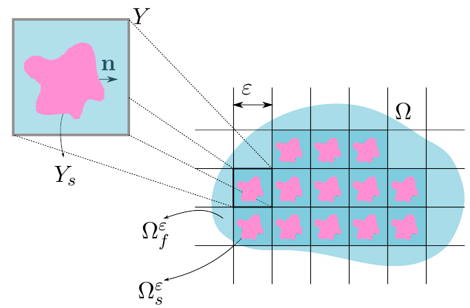
Figure 1: Reference cell $Y$ and domain $\Omega$.

2.3 The model

Denote by $\rho_{f},\rho_{s},\nu_{es},\mu$ and $\mathbf{g}$ the (mass) density of fluid, the density of inclusions, the electric conductivity of inclusions, the magnetic permeability and the external force field, respectively. The unknowns include the fluid velocity $\mathbf{u}^{\varepsilon}$, the fluid pressure $p^{\varepsilon}$ and the magnetic field $\mathbf{B}^{\varepsilon}$ (which in turn, determines the magnetising field $\mathbf{H}^{\varepsilon}$). For simplicity, we assume that the magnetic permeability is piecewise-constant and given by

$$\mu(x)=\begin{cases}\mu_{f},&\text{ if }x\in\Omega^{\varepsilon}_{f},\\ \mu_{s},&\text{ if }x\in\Omega^{\varepsilon}_{s},\end{cases}$$

where $\mu_{f},\,\mu_{s}>0$.

We consider the following non-linear system modeling a suspension of rigid inclusions in a non-conducting carrier fluid:

(1a) $$\rho_{f}\left[\frac{\partial\mathbf{u}^{\varepsilon}}{\partial t}+(\mathbf{u}^{\varepsilon}\cdot\nabla)\mathbf{u}^{\varepsilon}\right]-\operatorname{{div}}\boldsymbol{\sigma}^{\varepsilon} =\rho_{f}\mathbf{g} \text{ in }\Omega^{\varepsilon}_{f},$$

(1b) $$\operatorname{{div}}\mathbf{u}^{\varepsilon} =0 \text{ in }\Omega^{\varepsilon}_{f}$$

(1c) $${\mathbb{D}}(\mathbf{u}^{\varepsilon}) =0 \text{ in }\Omega^{\varepsilon}_{s},$$

(1d) $$\operatorname{{curl}}\mathbf{H}^{\varepsilon} =0 \text{ in }\Omega^{\varepsilon}_{f},$$

(1e) $$\frac{\partial\mathbf{B}^{\varepsilon}}{\partial t}+\frac{1}{\nu_{es}}\operatorname{{curl}}\operatorname{{curl}}\mathbf{H}^{\varepsilon} =\operatorname{{curl}}\left(\mathbf{u}^{\varepsilon}\times\mathbf{B}^{\varepsilon}\right) \text{ in }\Omega^{\varepsilon}_{s},$$

(1f) $$\operatorname{{div}}\mathbf{B}^{\varepsilon} =0 \text{ in }\Omega,$$

(1g) $$\mathbf{B}^{\varepsilon} =\mu\mathbf{H}^{\varepsilon} \text{ in }\Omega.$$

Suppose that the induced electric field is negligible, then the Lorentz force can be written as:

(2) $$\mathbf{f}^{\mathrm{mag}}=\operatorname{{curl}}\mathbf{H}^{\varepsilon}\times\mathbf{B}^{\varepsilon}=\begin{cases}0,&\text{ in }\Omega^{\varepsilon}_{f},\\ \operatorname{{curl}}\mathbf{H}^{\varepsilon}\times\mathbf{B}^{\varepsilon},&\text{ in }\Omega^{\varepsilon}_{s}.\end{cases}$$

Thus by the Law of Inertia [31, Axiom 5.2, page 171], we obtain the balance equations of force and torque:

(3a) $$\int_{Y_{i,s}}\rho_{s}\dot{\mathbf{u}^{\varepsilon}}\operatorname{d\!}x =\int_{\Gamma_{i}}\boldsymbol{\sigma}^{\varepsilon}(\mathbf{u}^{\varepsilon},p^{\varepsilon})\mathbf{n}\operatorname{d\!}\Gamma+\int_{Y_{i,s}}\operatorname{{curl}}\mathbf{H}^{\varepsilon}\times\mathbf{B}^{\varepsilon}\operatorname{d\!}x+\int_{Y_{i,s}}\rho_{s}\mathbf{g}\operatorname{d\!}x,$$

$$\int_{Y_{i,s}}\rho_{s}\left(x-{\mathrm{G}_{i}}\right)\times\dot{\mathbf{u}^{\varepsilon}}\operatorname{d\!}x =\int_{\Gamma_{i}}\left(x-{\mathrm{G}_{i}}\right)\times\boldsymbol{\sigma}^{\varepsilon}(\mathbf{u}^{\varepsilon},p^{\varepsilon})\mathbf{n}\operatorname{d\!}\Gamma$$

$$\qquad{}+{}\int_{Y_{i,s}}\left(x-{\mathrm{G}_{i}}\right)\times(\operatorname{{curl}}\mathbf{H}^{\varepsilon}\times\mathbf{B}^{\varepsilon})\operatorname{d\!}x$$

(3b) $$\qquad{}+{}\int_{Y_{i,s}}\rho_{s}\left(x-{\mathrm{G}_{i}}\right)\times\mathbf{g}\operatorname{d\!}x,$$

where $\dot{\mathbf{u}^{\varepsilon}}\coloneqq\frac{\partial\mathbf{u}^{\varepsilon}}{\partial t}+\left(\mathbf{u}^{\varepsilon}\cdot\nabla\right)\mathbf{u}^{\varepsilon}$ is the convective derivative, and $\mathrm{G}_{i}$ is the center of mass of the particle $Y_{i,s}$. The (outer) boundary conditions on the external boundary $\partial\Omega$ are

(4) $$\mathbf{u}^{\varepsilon}=0,\quad\operatorname{{curl}}\mathbf{H}^{\varepsilon}\times\mathbf{n}=0,\quad\mathbf{B}^{\varepsilon}\cdot\mathbf{n}=q,$$

where $\displaystyle\boldsymbol{\sigma}^{\varepsilon}(\mathbf{u}^{\varepsilon},p^{\varepsilon})\coloneqq 2\eta{\mathbb{D}}(\mathbf{u}^{\varepsilon})-p^{\varepsilon}I$, $\displaystyle{\mathbb{D}}(\mathbf{u}^{\varepsilon})\coloneqq\frac{\nabla\mathbf{u}^{\varepsilon}+\left(\nabla\mathbf{u}^{\varepsilon}\right)^{\top}}{2}$, and $q\in H^{1/2}(\partial\Omega)$ satisfying the compatibility condition $\int_{\partial\Omega}q\operatorname{d\!}\mathcal{H}^{d-1}=0.$ Since $\mu$ is piecewise-constant, from now on, we write:

$$\mathbf{H}^{\varepsilon}=\begin{cases}\displaystyle\frac{\mathbf{B}^{\varepsilon}}{\mu_{f}},&\text{ if }x\in\Omega^{\varepsilon}_{f},\\[12.0pt] \displaystyle\frac{\mathbf{B}^{\varepsilon}}{\mu_{s}},&\text{ if }x\in\Omega^{\varepsilon}_{s}.\end{cases}$$

2.4 Dimensional analysis

Let $L,U,B$, and $\mu_{s}$ be the characteristic scales corresponding to length, velocity, magnetic field and magnetic permeability, respectively. The characteristic time $T$ and body density force $F$ are defined by $T=\frac{L}{U}$ and $F=\frac{U^{2}}{L}.$

Let $x^{*}\coloneqq\frac{x}{L},\mathbf{u}^{\varepsilon*}\coloneqq\frac{\mathbf{u}}{U},p^{\varepsilon*}\coloneqq\frac{pL}{\eta U},\mathbf{g}^{*}\coloneqq\frac{\mathbf{g}L}{U^{2}}$ and $\mu^{*}\coloneqq\frac{\mu}{\mu_{s}}$. The dimensionless quantities that appear are the hydrodynamic Reynolds number ${R}_{{e}}=\frac{\rho_{f}UL}{\eta}$, the magnetic Reynolds number ${R}_{{m}}=\mu_{s}\nu_{es}UL$, the Alfven number ${A}_{{l}}=\frac{B^{2}L}{\eta\mu_{s}U}$, and the density ratio which, for simplicity, is assumed to satisfy $\frac{\rho_{s}}{\rho_{f}}=1$. Also, in the sequel, we drop the star to lighten the notation. The dimensionless versions of (1), (3) and (4) are:

(5a) $${R}_{{e}}\left[\frac{\partial\mathbf{u}^{\varepsilon}}{\partial t}+(\mathbf{u}^{\varepsilon}\cdot\nabla)\mathbf{u}^{\varepsilon}\right]-\operatorname{{div}}\boldsymbol{\sigma}^{\varepsilon}(\mathbf{u}^{\varepsilon},p^{\varepsilon}) ={R}_{{e}}\mathbf{g} \text{ in }\Omega^{\varepsilon}_{f},$$

(5b) $$\operatorname{{div}}\mathbf{u}^{\varepsilon} =0 \text{ in }\Omega^{\varepsilon}_{f}$$

(5c) $${\mathbb{D}}(\mathbf{u}^{\varepsilon}) =0 \text{ in }\Omega^{\varepsilon}_{s},$$

(5d) $$\operatorname{{curl}}\mathbf{B}^{\varepsilon} =0 \text{ in }\Omega^{\varepsilon}_{f},$$

(5e) $$\frac{\partial\mathbf{B}^{\varepsilon}}{\partial t}+\frac{1}{{R}_{{m}}}\operatorname{{curl}}\operatorname{{curl}}\mathbf{B}^{\varepsilon} =\operatorname{{curl}}\left(\mathbf{u}^{\varepsilon}\times\mathbf{B}^{\varepsilon}\right) \text{ in }\Omega^{\varepsilon}_{s},$$

(5f) $$\operatorname{{div}}\mathbf{B}^{\varepsilon} =0 \text{ in }\Omega.$$

equipped with the balance equations:

$${R}_{{e}}\int_{Y^{\varepsilon}_{i,s}}\dot{\mathbf{u}^{\varepsilon}}\operatorname{d\!}x =\int_{\Gamma^{\varepsilon}_{i}}\boldsymbol{\sigma}^{\varepsilon}(\mathbf{u}^{\varepsilon},p^{\varepsilon})\mathbf{n}\operatorname{d\!}\mathcal{H}^{d-1}$$

(6a) $$\qquad{}+{}{A}_{{l}}\int_{Y^{\varepsilon}_{i,s}}\operatorname{{curl}}\mathbf{B}^{\varepsilon}\times\mathbf{B}^{\varepsilon}\operatorname{d\!}x+{R}_{{e}}\int_{Y^{\varepsilon}_{i,s}}\mathbf{g}\operatorname{d\!}x,$$

$${R}_{{e}}\int_{Y^{\varepsilon}_{i,s}}\left(x-{\mathrm{G}^{\varepsilon}_{i}}\right)\times\dot{\mathbf{u}^{\varepsilon}}\operatorname{d\!}x =\int_{\Gamma^{\varepsilon}_{i}}\left(x-{\mathrm{G}^{\varepsilon}_{i}}\right)\times\boldsymbol{\sigma}^{\varepsilon}(\mathbf{u}^{\varepsilon},p^{\varepsilon})\mathbf{n}\operatorname{d\!}\mathcal{H}^{d-1}+$$

$$\qquad{}+{}{A}_{{l}}\int_{Y^{\varepsilon}_{i,s}}\left(x-{\mathrm{G}^{\varepsilon}_{i}}\right)\times(\operatorname{{curl}}\mathbf{B}^{\varepsilon}\times\mathbf{B}^{\varepsilon})\operatorname{d\!}x$$

(6b) $$\qquad{}+{}{R}_{{e}}\int_{Y^{\varepsilon}_{i,s}}\left(x-{\mathrm{G}^{\varepsilon}_{i}}\right)\times\mathbf{g}\operatorname{d\!}x,$$

and the boundary conditions:

(7) $$\mathbf{u}^{\varepsilon}=0,\quad\operatorname{{curl}}\mathbf{B}^{\varepsilon}\times\mathbf{n}=0,\quad\mathbf{B}^{\varepsilon}\cdot\mathbf{n}=q,$$

where now $\displaystyle\boldsymbol{\sigma}^{\varepsilon}(\mathbf{u}^{\varepsilon},p^{\varepsilon})\coloneqq 2{\mathbb{D}}(\mathbf{u}^{\varepsilon})-p^{\varepsilon}{\mathbf{I}}$.

Hereafter, we consider the stationary flow, i.e., the time derivative is ignored:

(8a) $${R}_{{e}}(\mathbf{u}^{\varepsilon}\cdot\nabla)\mathbf{u}^{\varepsilon}-\operatorname{{div}}\boldsymbol{\sigma}^{\varepsilon}(\mathbf{u}^{\varepsilon},p^{\varepsilon}) ={R}_{{e}}\mathbf{g} \text{ in }\Omega^{\varepsilon}_{f},$$

(8b) $$\operatorname{{div}}\mathbf{u}^{\varepsilon} =0 \text{ in }\Omega^{\varepsilon}_{f},$$

(8c) $${\mathbb{D}}(\mathbf{u}^{\varepsilon}) =0 \text{ in }\Omega_{s}^{\varepsilon},$$

(8d) $$\operatorname{{curl}}\mathbf{B}^{\varepsilon} =0 \text{ in }\Omega_{f}^{\varepsilon},$$

(8e) $$\frac{1}{{R}_{{m}}}\operatorname{{curl}}\operatorname{{curl}}\mathbf{B}^{\varepsilon}-\operatorname{{curl}}\left(\mathbf{u}^{\varepsilon}\times\mathbf{B}^{\varepsilon}\right) =\mathbf{h} \text{ in }\Omega^{\varepsilon}_{s},$$

(8f) $$\operatorname{{div}}\mathbf{B}^{\varepsilon} =0 \text{ in }\Omega.$$

equipped with the balance equations:

$${R}_{{e}}\int_{Y^{\varepsilon}_{i,s}}(\mathbf{u}^{\varepsilon}\cdot\nabla)\mathbf{u}^{\varepsilon} =\int_{\Gamma^{\varepsilon}_{i}}\boldsymbol{\sigma}^{\varepsilon}\mathbf{n}\operatorname{d\!}\mathcal{H}^{d-1}$$

(9a) $$\qquad{}+{}{A}_{{l}}\int_{Y^{\varepsilon}_{i,s}}\operatorname{{curl}}\mathbf{B}^{\varepsilon}\times\mathbf{B}^{\varepsilon}\operatorname{d\!}x+{R}_{{e}}\int_{Y^{\varepsilon}_{i,s}}\mathbf{g}\operatorname{d\!}x,$$

$${R}_{{e}}\int_{Y^{\varepsilon}_{i,s}}(x-\mathrm{G}^{\varepsilon}_{i})\times(\mathbf{u}^{\varepsilon}\cdot\nabla)\mathbf{u}^{\varepsilon} =\int_{\Gamma^{\varepsilon}_{i}}\left(x-\mathrm{G}^{\varepsilon}_{i}\right)\times\boldsymbol{\sigma}^{\varepsilon}\mathbf{n}\operatorname{d\!}\mathcal{H}^{d-1}$$

$$\qquad{}+{}{A}_{{l}}\int_{Y^{\varepsilon}_{i,s}}\left(x-\mathrm{G}_{i}^{\varepsilon}\right)\times\left(\operatorname{{curl}}\mathbf{B}^{\varepsilon}\times\mathbf{B}^{\varepsilon}\right)\operatorname{d\!}x$$

(9b) $$\qquad{}+{}{R}_{{e}}\int_{Y^{\varepsilon}_{i,s}}(x-\mathrm{G}^{\varepsilon}_{i})\times\mathbf{g}\operatorname{d\!}x,$$

the boundary conditions

(10) $$\mathbf{u}^{\varepsilon}=0,\quad\operatorname{{curl}}\mathbf{B}^{\varepsilon}\times\mathbf{n}=0,\quad\mathbf{B}^{\varepsilon}\cdot\mathbf{n}=0$$

and the compatibility condition

(11) $$\int_{\Omega_{s}}\mathbf{h}\cdot\nabla\psi\operatorname{d\!}x=0\text{ for all }\nabla\psi\in H^{1}_{n}(\Omega,{\mathbb{R}}^{d}).$$

We note that the function $\mathbf{h}\in L^{2}(\Omega,{\mathbb{R}}^{d})$ appears in (8e) due to a lifting of the non-homogeneous magnetic condition (4) to the homogeneous condition (10), i.e. substracting $\mathbf{B}^{\varepsilon}$ by a suitable function, see [36], and [29, Section 3.8]. Here, $H^{1}_{n}(\Omega,{\mathbb{R}}^{d})$ is the set of weakly differentiable functions from $\Omega$ to ${\mathbb{R}}^{d}$ with vanishing normal trace, see Section 2.5.1 below.

2.5 Useful results from functional analysis

In this section, we collect some background results from functional analysis used in the sequel. We separate the functional spaces and theorems of the two-scale convergence method from the ones of saddle point problems to make it easier to keep track.

2.5.1 Abstract framework for our non-linear problem

The results for linear saddle point problems date back to the seminal works by I. Babuška and F. Brezzi, c.f. [4, 10]. They are then adapted to the non-linear cases such as the Navier-Stokes equations and magnetorhydrodynamic equations, c.f. [30, 54, 36, 29, 35]. We summarize here the results used in our paper and refer the readers to the works cited above for their proofs.

Let $X$ and $P$ be two real Hilbert spaces, and $f\in X$. Let $a(\,\cdot\,;\cdot,\cdot)\colon X\times X\times X\to{\mathbb{R}}$ be a non-linear form such that for any $w\in X$, $a(w;\cdot,\cdot)$ is a bilinear continuous form on $X\times X$. Let $b\colon X\times P\to{\mathbb{R}}$ be a continuous bilinear form. Consider the following non-linear problem:

Find $(u,p)\in X\times P$, such that for all $(v,q)\in X\times P$,

(12a) $$a(u;u,v)+b(v,p) =\left\langle f,v\right\rangle,$$

(12b) $$b(u,q) =0,$$

where $\langle\cdot,\cdot\rangle$ is the dual pairing. The unknown $p$ can be regarded as the Lagrange multiplier associated with the constraint (12b). The idea is to embed the constraint (12b) into $X$ by introducing the space

$$M=\left\{u\in X\colon b(u,q)=0\text{ for all }q\in P\right\},$$

and consider a simpler problem that reads: Find $u\in M$ such that for all $v\in M,$

(13) $$a(u;u,v)=\left\langle f,v\right\rangle.$$

The continuity of $b$ implies that $M$ is a closed linear subspace of $X$, and, thus, $M$ is also a Hilbert space.

Theorem 2.1 (Existence and uniqueness of solution of (13)).

If the following conditions hold:

1. there exists $\alpha>0$ such that for all $v\in M$,

   (14) $$a(v;v,v)\geq\alpha\left\lVert v\right\rVert^{2}_{X};$$

2. the space $M$ is separable and such that for any sequence $v_{n}$ that weakly converges to $v$ in $M$, $a(v_{n};v_{n},w)$ converges to $a(v;v,w)$, for all $w\in M$;

then there exists at least one solution of problem (13): $u\in M$. If in addition, we assume that:

1. the elliptic property (i) holds uniformly with respect to the first variable, i.e. there exists $\alpha>0$ such that for all $v,w\in M$,

   (15) $$a(w;v,v)\geq\alpha\left\lVert v\right\rVert^{2}_{X},$$

2. there exists a constant $\gamma>0$ such that, for all $u_{1},u_{2},v,w\in M$,

   (16) $$\left\lvert a(u_{2};v,w)-a(u_{1};v,w)\right\rvert\leq\gamma\left\lVert u_{2}-u_{1}\right\rVert_{X}\left\lVert v\right\rVert_{X}\left\lVert w\right\rVert_{X},$$

then problem (13) has a unique solution $u\in M$, provided that

(17) $$\frac{\gamma\left\lVert w\right\rVert_{M}}{\alpha^{2}}<1,$$

where $w\in M$ is such that $\langle f|_{M},v\rangle=(w,v)_{X},~{}\forall v\in M$, with $f|_{M}$ being the restriction of $f$ on $M$.

Theorem 2.1 allows us to establish the existence and uniqueness of the solution $u$ of (13). To recover the unknown $p$ that solves (12), we need to introduce the following definition.

Definition 2.2.

The following is called the inf-sup condition or the Babuška-Brezzi condition or the Ladyzhenskaya-Babuška-Brezzi condition:

(18) $$\exists\,\beta>0\quad\text{ such that }\quad\inf_{q\in P\setminus\left\{0\right\}}\sup_{v\in X\setminus\left\{0\right\}}\frac{b(v,q)}{\left\lVert v\right\rVert_{X}\left\lVert q\right\rVert_{P}}\geq\beta.$$

If the bilinear form $b$ in (12) satisfies the inf-sup condition (18) then, by the Riesz Representation Theorem and the Closed Range Theorem [13], the existence and uniqueness of the solution $u$ of (13) implies the existence and uniqueness of the solution $(u,p)$ of (12).

The inf-sup condition can be verified by

Proposition 2.3.

Let $B\colon X\to P$ be the continuous linear operator associated to the continuous bilinear form $b$ by $(Bv,q)_{P}=b(v,q)$ for all $(v,q)\in X\times P$ (here we use the Riesz Representation Theorem). Then the following statements are equivalent:

1. The inf-sup condition (18) holds.

2. $B^{\top}\colon P\to X$ is injective and $B^{\top}$ has a closed range. Here $B^{\top}$ is the transpose of $B$, i.e. $(v,B^{\top}q)_{X}=(Bv,q)_{P}$ for all $(v,q)\in X\times P.$

3. $B\colon X\to P$ is surjective.

2.5.2 The two-scale convergence method

Two-scale convergence was invented by G. Nguetseng and further developed by G. Allaire. We collect here the important notions and results relevant to this paper, whose proofs can be found in [11, 57, 38, 39]. The following spaces are used in the paper below.

• $C_{\mathrm{per}}(Y)$ – the subspace of $C({\mathbb{R}}^{d})$ of $Y$-periodic functions;

• $C^{\infty}_{\mathrm{per}}(Y)$ – the subspace of $C^{\infty}({\mathbb{R}}^{d})$ of $Y$-periodic functions;

• $H^{1}_{\mathrm{per}}(Y)$ – the closure of $C^{\infty}_{\mathrm{per}}(Y)$ in the $H^{1}$-norm;

• $\mathcal{D}(\Omega,X)$ – where $X$ is a Banach space – the space infinitely differentiable functions from $\Omega$ to $X$, whose support is a compact set of $\mathbb{R}^{d}$ contained in $\Omega$.

• $L^{p}(\Omega,X)$ – where $X$ is a Banach space and $1\leq p\leq\infty$ – the space of measurable functions $w\colon x\in\Omega\mapsto w(x)\in X$ such that $\left\lVert w\right\rVert_{L^{p}(\Omega,X)}\coloneqq\left(\int_{\Omega}\left\lVert w(x)\right\rVert^{p}_{X}\operatorname{d\!}x\right)^{\frac{1}{p}}<\infty.$

• $L^{p}_{\mathrm{per}}\left(Y,C(\bar{\Omega})\right)$ – the space of measurable functions $w\colon y\in Y\mapsto w(\cdot,y)\in C(\bar{\Omega})$, such that $w$ is periodic with respect to $y$ and $\int_{Y}\left(\sup_{x\in\bar{\Omega}}\left\lvert w(x,y)\right\rvert\right)^{p}\operatorname{d\!}y<\infty.$

Definition 2.4 ($L^{p}-$admissible test function).

Let $1\leq p<+\infty$. A function $\psi\in L^{p}(\Omega\times Y)$, $Y$-periodic in the second component, is called an $L^{p}-$admissible test function if for all $\varepsilon>0$, $\psi\left(\cdot,\frac{\cdot}{\varepsilon}\right)$ is measurable and

(19) $$\lim_{\varepsilon\to 0}\int_{\Omega}\left\lvert\psi\left(x,\frac{x}{\varepsilon}\right)\right\rvert^{p}\operatorname{d\!}x=\frac{1}{\left\lvert Y\right\rvert}\int_{\Omega}\int_{Y}\left\lvert\psi(x,y)\right\rvert^{p}\operatorname{d\!}y\operatorname{d\!}x.$$

It is known that functions belonging to the spaces $\mathcal{D}\left(\Omega,C_{\mathrm{per}}^{\infty}(Y)\right)$, $C\left(\bar{\Omega},C_{\mathrm{per}}(Y)\right)$, $L^{p}_{\mathrm{per}}\left(Y,C(\bar{\Omega})\right)$ or $L^{p}\left(\Omega,C_{\mathrm{per}}(Y)\right)$ are admissible [3], but the precise characterization of those admissible test functions is still an open question.

Definition 2.5.

A sequence $\{v^{\varepsilon}\}_{\varepsilon>0}$ in $L^{2}(\Omega)$ is said to two-scale converge to $v=v(x,y)$, with $v\in L^{2}(\Omega\times Y)$, and we write $v^{\varepsilon}\xrightharpoonup{~{}2~{}}v$, if and only if:

(20) $$\lim_{\varepsilon\to 0}\int_{\Omega}v^{\varepsilon}(x)\psi\left(x,\frac{x}{\varepsilon}\right)\operatorname{d\!}x=\frac{1}{\left\lvert Y\right\rvert}\int_{\Omega}\int_{Y}v(x,y)\psi(x,y)\operatorname{d\!}y\operatorname{d\!}x,$$

for any test function $\psi=\psi(x,y)$ with $\psi\in\mathcal{D}\left(\Omega,C_{\mathrm{per}}^{\infty}(Y)\right)$.

In (20), we can choose $\psi$ be any ($L^{2}-$)admissible test function. Any bounded sequence $v^{\varepsilon}\in L^{2}(\Omega)$ has a subsequence that two-scale converges to a limit $v^{0}\in L^{2}(\Omega\times Y)$. Moreover, from [3, Theorem 1.8, Remark 1.10 and Corollary 5.4], we have

Theorem 2.6 (Corrector result).

Let $u^{\varepsilon}$ be a sequence of functions in $L^{2}(\Omega)$ that two-scale converges to a limit $u^{0}(x,y)\in L^{2}(\Omega\times Y)$. Assume that

(21) $$\lim_{\varepsilon\to 0}\left\lVert u^{\varepsilon}\right\rVert_{L^{2}(\Omega)}=\left\lVert u^{0}\right\rVert_{L^{2}(\Omega\times Y)}.$$

Then for any sequence $v^{\varepsilon}$ in $L^{2}(\Omega)$ that two-scale converges to $v^{0}\in L^{2}(\Omega\times Y),$ one has

$$u^{\varepsilon}v^{\varepsilon}\xrightharpoonup[\hphantom{~{}2~{}}]{}\frac{1}{\left\lvert Y\right\rvert}\int_{Y}u^{0}(x,y)v^{0}(x,y)\operatorname{d\!}x\operatorname{d\!}y\text{ in }\mathcal{D}^{\prime}(\Omega)$$

Furthermore, if $u^{0}(x,y)$ belongs to $L^{2}\left(\Omega,C_{\mathrm{per}}(Y)\right)$ or $L^{2}_{\mathrm{per}}\left(Y,C(\Omega)\right)$, then

(22) $$\lim_{\varepsilon\to 0}\left\lVert u^{\varepsilon}(x)-u^{0}\left(x,\frac{x}{\varepsilon}\right)\right\rVert_{L^{2}(\Omega)}=0.$$

In fact, the smoothness assumption on $u^{0}$ in (22) is needed only for $u^{0}\left(x,\frac{x}{\varepsilon}\right)$ is to be measurable and to belong to $L^{2}(\Omega)$. Finally, we recall that if $\psi\in L^{2}(\Omega\times Y)$ is a Carathéodory function then $\psi\left(\cdot,\frac{\cdot}{\varepsilon}\right)$ is measurable. This fact is used later on to prove that $\mathds{1}_{\Omega\times Y_{s}}$ is an admissible test function.

3 Main results

We now define the admissible spaces on the $C^{1,1}-$domain $\Omega$ for the fluid velocity $\mathbf{u}^{\varepsilon}$, the magnetic field $\mathbf{B}^{\varepsilon}$ and the fluid pressure $p^{\varepsilon}$. Let

$$H^{1}_{n}(\Omega,{\mathbb{R}}^{d}) \coloneqq\left\{\mathbf{C}\in H^{1}(\Omega,{\mathbb{R}}^{d})\colon\mathbf{C}\cdot\mathbf{n}_{\partial\Omega}=0\right\},$$

$$L_{0}^{2}(\Omega) \coloneqq\left\{q\in L^{2}(\Omega)\colon\int_{\Omega}q\operatorname{d\!}x=0\right\},$$

$$\mathfrak{H} \coloneqq\left\{\mathbf{C}\in L^{2}(\Omega,{\mathbb{R}}^{d})\colon\operatorname{{curl}}\mathbf{C}\in L^{2}(\Omega,{\mathbb{R}}^{d}),\operatorname{{div}}\mathbf{C}\in L^{2}(\Omega),\mathbf{C}\cdot\mathbf{n}_{\partial\Omega}=0\right\},$$

$$\mathfrak{V}^{\varepsilon} \coloneqq\left\{\mathbf{v}\in H_{0}^{1}(\Omega,{\mathbb{R}}^{d})\colon{\mathbb{D}}(\mathbf{v})=0\text{ in }\Omega_{s}^{\varepsilon}\right\},$$

$$\mathfrak{P}^{\varepsilon} \coloneqq\operatorname{{div}}(\mathfrak{V}^{\varepsilon})=\left\{q\in L_{0}^{2}(\Omega)\colon\exists\mathbf{v}\in\mathfrak{V}^{\varepsilon}\text{ such that }q=\operatorname{{div}}\mathbf{v}\right\},$$

$$\mathfrak{U}^{\varepsilon} \coloneqq\left\{\mathbf{v}\in H_{0}^{1}(\Omega,{\mathbb{R}}^{d})\colon{\mathbb{D}}(\mathbf{v})=0\text{ in }\Omega_{s}^{\varepsilon},~{}\operatorname{{div}}\mathbf{v}=0\text{ in }\Omega^{\varepsilon}_{f}\right\},$$

$$\mathfrak{X}^{\varepsilon} \coloneqq\mathfrak{V}^{\varepsilon}\times\left\{\mathbf{C}\in H^{1}_{n}(\Omega,{\mathbb{R}}^{d})\colon\operatorname{{curl}}\mathbf{C}=0\text{ in }\Omega^{\varepsilon}_{f}\right\},$$

$$\mathfrak{Y}^{\varepsilon} \coloneqq\mathfrak{U}^{\varepsilon}\times\left\{\mathbf{C}\in H^{1}_{n}(\Omega,{\mathbb{R}}^{d})\colon\operatorname{{curl}}\mathbf{C}=0\text{ in }\Omega^{\varepsilon}_{f}\right\}.$$

These spaces are equipped with natural Sobolev norms. Moreover, given normed spaces $A$ and $B$, the norm of its product space $A\times B$ is defined by $\left\lVert(a,b)\right\rVert^{2}_{A\times B}\coloneqq\left\lVert a\right\rVert_{A}^{2}+\left\lVert b\right\rVert_{B}^{2}$ for $a\in A,b\in B.$

As we will see later, to utilize the framework presented in Section 2.5.1, we choose $X=\mathfrak{X}^{\varepsilon}$, $M=\mathfrak{Y}^{\varepsilon}$, and $P=\mathfrak{P}^{\varepsilon}$.

In addition, let $\kappa_{GR}^{-1}$, be the norm of the embedding $\mathfrak{H}\to H^{1}$, $\kappa_{S}$ the norm of the Sobolev embedding $H^{1}\to L^{4}$, and $\kappa_{K}^{-1}$ the constant in Korn’s inequality, respectively. Then the main result of this paper is summarized in the following theorem.

Theorem 3.1.

Suppose the data $\mathbf{g}$ and $\mathbf{h}$ are small enough such that

(23) $${R}_{{e}}\left\lVert\mathbf{g}\right\rVert_{L^{2}}+{A}_{{l}}\left\lVert\mathbf{h}\right\rVert_{L^{2}}\leq\frac{\left(\min\left\{\frac{{A}_{{l}}}{{R}_{{m}}}\kappa_{GR},\kappa_{K}\right\}\right)^{2}}{\kappa_{S}\max\left\{1,2{A}_{{l}}\right\}}.$$

Then, for $\varepsilon>0$, the system (8) has a unique solution $\mathbf{u}^{\varepsilon}\in H_{0}^{1}(\Omega,{\mathbb{R}}^{d}),$ $p^{\varepsilon}\in L_{0}^{2}(\Omega)$, $\mathbf{B}^{\varepsilon}\in H_{n}^{1}(\Omega,{\mathbb{R}}^{d})$. Moreover, there exist a constant, symmetric and elliptic fourth rank tensor $\mathcal{N}$, and two constant, symmetric and elliptic matrices $\mathcal{M},\mathcal{E}$ such that

$$\mathbf{u}^{\varepsilon}\xrightharpoonup[\hphantom{~{}2~{}}]{}\mathbf{u}^{0}\text{ in }H^{1}(\Omega,{\mathbb{R}}^{d}),\quad\mathbf{B}^{\varepsilon}\xrightharpoonup[\hphantom{~{}2~{}}]{}\mathbf{B}^{0}\text{ in }H^{1}(\Omega,{\mathbb{R}}^{d}),\quad p^{\varepsilon}\xrightharpoonup[\hphantom{~{}2~{}}]{}\Pi\text{ in }L^{2}_{0}(\Omega$$

where $\mathbf{u}^{0}\in H_{0}^{1}(\Omega,{\mathbb{R}}^{d})$, $\Pi\in L_{0}^{2}(\Omega)$, and $\mathbf{B}^{0}\in H_{n}^{1}(\Omega,{\mathbb{R}}^{d})$ satisfy the following effective system of equations all defined on the domain $\Omega$,

(24) $$\begin{split}\operatorname{{div}}\mathbf{u}^{0}=\operatorname{{div}}\mathbf{B}^{0}&=0,\\ \left(\mathbf{u}^{0}\cdot\nabla\right)\mathbf{u}^{0}-\operatorname{{div}}\left(2\mathcal{N}_{ijmn}\left[{\mathbb{D}}(\mathbf{u}^{0})\right]_{ij}\mathrm{e}^{m}\otimes\mathrm{e}^{n}-\Pi\,{\mathbf{I}}\right)&={R}_{{e}}\mathbf{g}+{A}_{{l}}\frac{\left\lvert Y_{s}\right\rvert}{\left\lvert Y\right\rvert}\operatorname{{curl}}\mathbf{B}^{0}\times\mathbf{B}^{0},\\ \frac{1}{{R}_{{m}}}\operatorname{{curl}}\left(\mathcal{M}_{jn}\epsilon_{ijk}\frac{\partial B^{0}_{i}}{\partial x_{k}}\mathrm{e}^{n}\right)-\operatorname{{curl}}\left(\mathcal{E}_{kn}\epsilon_{ijk}u^{0}_{i}B^{0}_{j}\mathrm{e}^{n}\right)&=\frac{\left\lvert Y_{s}\right\rvert}{\left\lvert Y\right\rvert}\mathbf{h}.\end{split}$$

The road map of the proof of Theorem 3.1 goes as follows:

• First, we present the variational formulation for problem (8)–(11) and prove their equivalence in Section 3.1.

• Second, the existence and a priori estimates for the fine-scale velocity $\mathbf{u}^{\varepsilon}$ and the magnetic field $\mathbf{B}^{\varepsilon}$ are established in Section 3.2, thanks to Theorem 2.1. The first two steps are adapted from the classical theory of magnetohydrodynamics, c.f. [30, 54, 36, 29, 35]. In particular, the presentation of those two steps is inspired by [29, 54, 36].

• Third, in Section 3.3, the existence and a priori estimate for the fine-scale pressure $p^{\varepsilon}$ are recovered by an inf-sup condition. A construction based on the Bogovskiĭ map allows us to control the norm of the pressure $p^{\varepsilon}$ uniformly with respect to $\varepsilon$, c.f. [2, 1, 21, 20, 18, 5, 41].

• Next, the two-scale homogenized problem is derived in Section 3.4. Here, a corrector result of two-scale convergence [3] is crucial for passing to the limit of several integrals over a changing domain.

• Finally, the local and homogenized problems are recovered in Section 3.5 and Section 3.6. Explicit formulas for the effective viscosity $\mathcal{N}$, the effective magnetic reluctivity $\mathcal{M}$ and the effective electric conductivity $\mathcal{E}$ are provided in (82).

3.1 Variational formulation

We define bilinear, trilinear, and linear forms $\mathcal{A}^{\varepsilon}(\cdot,\cdot):\mathfrak{X}^{\varepsilon}\times\mathfrak{X}^{\varepsilon}\to\mathbb{R}$, $\mathcal{B}^{\varepsilon}(\cdot,\cdot):\mathfrak{X}^{\varepsilon}\times\mathfrak{P}^{\varepsilon}\to\mathbb{R}$, and $\mathcal{C}^{\varepsilon}(\cdot,\cdot,\cdot):\mathfrak{X}^{\varepsilon}\times\mathfrak{X}^{\varepsilon}\times\mathfrak{X}^{\varepsilon}\to\mathbb{R}$, $\mathcal{L}^{\varepsilon}(\cdot):\mathfrak{X}^{\varepsilon}\to\mathbb{R}$ by

$$\mathcal{A}^{\varepsilon}\left((\mathbf{u},\mathbf{B}),(\mathbf{v},\mathbf{C})\right) \coloneqq 2\int_{\Omega^{\varepsilon}_{f}}{\mathbb{D}}(\mathbf{u}):{\mathbb{D}}(\mathbf{v})\operatorname{d\!}x$$

$${}+{}\frac{{A}_{{l}}}{{R}_{{m}}}\left[\int_{\Omega}\operatorname{{div}}\mathbf{B}\cdot\operatorname{{div}}\mathbf{C}\operatorname{d\!}x+\int_{\Omega^{\varepsilon}_{s}}\operatorname{{curl}}\mathbf{B}\cdot\operatorname{{curl}}\mathbf{C}\operatorname{d\!}x\right],$$

$$\mathcal{B}^{\varepsilon}\left((\mathbf{v},\mathbf{C}),p\right) \coloneqq\int_{\Omega}p\operatorname{{div}}\mathbf{v}\operatorname{d\!}x,$$

$$\mathcal{C}^{\varepsilon}\left((\mathbf{u}_{1},\mathbf{C}_{1}),(\mathbf{u}_{2},\mathbf{C}_{2}),(\mathbf{u}_{3},\mathbf{C}_{3})\right) \coloneqq{R}_{{e}}\int_{\Omega}\left(\mathbf{u}_{1}\cdot\nabla\right)\mathbf{u}_{2}\cdot\mathbf{u}_{3}\operatorname{d\!}x$$

$${}-{}{A}_{{l}}\int_{\Omega^{\varepsilon}_{s}}\left[(\operatorname{{curl}}\mathbf{C}_{2}\times\mathbf{C}_{1})\cdot\mathbf{u}_{3}\right.$$

$$\qquad{}+{}\left.\left(\mathbf{u}_{2}\times\mathbf{C}_{1}\right)\cdot\operatorname{{curl}}\mathbf{C}_{3}\right]\operatorname{d\!}x,$$

$$\mathcal{L}^{\varepsilon}(\mathbf{v},\mathbf{C}) \coloneqq{R}_{{e}}\int_{\Omega}\mathbf{g}\cdot\mathbf{v}\operatorname{d\!}x+{A}_{{l}}\int_{\Omega^{\varepsilon}_{s}}\mathbf{h}\cdot\mathbf{C}\operatorname{d\!}x.$$

We consider the weak formulation of problem (8):

Find $\left((\mathbf{u}^{\varepsilon},\mathbf{B}^{\varepsilon}),p^{\varepsilon}\right)\in\mathfrak{X}^{\varepsilon}\times\mathfrak{P}^{\varepsilon}$ such that for all $\left((\mathbf{v},\mathbf{C}),q\right)\in\mathfrak{X}^{\varepsilon}\times\mathfrak{P}^{\varepsilon}$,

(25) $$\begin{split}\mathcal{A}^{\varepsilon}\left((\mathbf{u}^{\varepsilon},\mathbf{B}^{\varepsilon}),(\mathbf{v},\mathbf{C})\right)+\mathcal{B}^{\varepsilon}\left((\mathbf{v},\mathbf{C}),p^{\varepsilon}\right)+\mathcal{C}^{\varepsilon}\left((\mathbf{u}^{\varepsilon},\mathbf{B}^{\varepsilon}),(\mathbf{u}^{\varepsilon},\mathbf{B}^{\varepsilon}),(\mathbf{v},\mathbf{C})\right)&=\mathcal{L}^{\varepsilon}(\mathbf{v},\mathbf{C}),\\ \mathcal{B}^{\varepsilon}\left((\mathbf{u}^{\varepsilon},\mathbf{B}^{\varepsilon}),q\right)&=0.\end{split}$$

Before showing that the weak formulation (25) is equivalent to the strong formulation (8), we recall:

Lemma 3.2 (Lemma 3.17 [29]).

If $\mathbf{B}\in H^{1}_{n}(\Omega,{\mathbb{R}}^{d})$, then there exists $\psi\in H^{2}(\Omega)$ such that

(26) $$\left\{\begin{array}[]{r l l}-\Delta\psi&\displaystyle=\operatorname{{div}}\mathbf{B}&\text{ in }\Omega,\\[1.0pt] \displaystyle\frac{\partial\psi}{\partial n}&\displaystyle=0&\text{ on }\partial\Omega.\end{array}\right.$$

In particular, $\nabla\psi\in H^{1}_{n}(\Omega,{\mathbb{R}}^{d})$.

Proposition 3.3.

Suppose that $\mathbf{h}$ satisfies (11). Then $\left((\mathbf{u}^{\varepsilon},\mathbf{B}^{\varepsilon}),p^{\varepsilon}\right)\in\mathfrak{X}^{\varepsilon}\times\mathfrak{P}^{\varepsilon}$ is a weak solution of (25) if and only if it is a solution of (8)-(10).

Proof 3.4.

The incompressibility condition (8b) is straightforward from the second equation of (25). We rewrite the first equation of (25) as

(27) $$\begin{split}&2\int_{\Omega^{\varepsilon}_{f}}{\mathbb{D}}(\mathbf{u}^{\varepsilon}):{\mathbb{D}}(\mathbf{v})\operatorname{d\!}x+\frac{{A}_{{l}}}{{R}_{{m}}}\left[\int_{\Omega}\operatorname{{div}}\mathbf{B}^{\varepsilon}\cdot\operatorname{{div}}\mathbf{C}\operatorname{d\!}x+\int_{\Omega^{\varepsilon}_{s}}\operatorname{{curl}}\mathbf{B}^{\varepsilon}\cdot\operatorname{{curl}}\mathbf{C}\operatorname{d\!}x\right]\\ &{}+{}\int_{\Omega}p^{\varepsilon}\operatorname{{div}}\mathbf{v}\operatorname{d\!}x{}+{}{R}_{{e}}\int_{\Omega}\left(\mathbf{u}^{\varepsilon}\cdot\nabla\right)\mathbf{u}^{\varepsilon}\cdot\mathbf{v}\operatorname{d\!}x\\ &{}-{}{A}_{{l}}\int_{\Omega^{\varepsilon}_{s}}(\operatorname{{curl}}\mathbf{B}^{\varepsilon}\times\mathbf{B}^{\varepsilon})\cdot\mathbf{v}\operatorname{d\!}x-{A}_{{l}}\int_{\Omega^{\varepsilon}_{s}}\left(\mathbf{u}^{\varepsilon}\times\mathbf{B}^{\varepsilon}\right)\cdot\operatorname{{curl}}\mathbf{C}\operatorname{d\!}x\\ &={R}_{{e}}\int_{\Omega}\mathbf{g}\cdot\mathbf{v}\operatorname{d\!}x+{A}_{{l}}\int_{\Omega^{\varepsilon}_{s}}\mathbf{h}\cdot\mathbf{C}\operatorname{d\!}x.\end{split}$$

Let $\mathbf{C}=0$ and choose $\mathbf{v}\in C^{\infty}_{c}(\Omega^{\varepsilon}_{f},{\mathbb{R}}^{d})$, then using integration by parts, we obtain (8a). Setting $\mathbf{C}=0$ again and choosing $\mathbf{v}\in H_{0}^{1}(\Omega,{\mathbb{R}}^{d})$ with ${\mathbb{D}}(\mathbf{v})=0$ on $\Omega^{\varepsilon}_{s}$, we obtain the balance equations (9).

Next, choosing $\mathbf{v}=0$ in (27) results in

(28) $$\begin{split}\frac{{A}_{{l}}}{{R}_{{m}}}\left[\int_{\Omega}\operatorname{{div}}\mathbf{B}^{\varepsilon}\cdot\operatorname{{div}}\mathbf{C}\operatorname{d\!}x+\int_{\Omega_{s}}\operatorname{{curl}}\mathbf{B}^{\varepsilon}\cdot\operatorname{{curl}}\mathbf{C}\operatorname{d\!}x\right]\\ -{A}_{{l}}\int_{\Omega_{s}}\left(\mathbf{u}^{\varepsilon}\times\mathbf{B}^{\varepsilon}\right)\cdot\operatorname{{curl}}\mathbf{C}\operatorname{d\!}x={A}_{{l}}\int_{\Omega_{s}}\mathbf{h}\cdot\mathbf{C}\operatorname{d\!}x.\end{split}$$

Let $\psi$ as in Lemma 3.2 and select $\mathbf{C}=\nabla\psi$ in (28), then by (11),

$$-\frac{{A}_{{l}}}{{R}_{{m}}}\int_{\Omega}(\operatorname{{div}}\mathbf{B}^{\varepsilon})^{2}\operatorname{d\!}x=0$$

so we obtain (8f). Therefore, (28) is simplified to

$$\frac{1}{{R}_{{m}}}\int_{\Omega_{s}}\operatorname{{curl}}\mathbf{B}^{\varepsilon}\cdot\operatorname{{curl}}\mathbf{C}\operatorname{d\!}x-\int_{\Omega_{s}}\left(\mathbf{u}^{\varepsilon}\times\mathbf{B}^{\varepsilon}\right)\cdot\operatorname{{curl}}\mathbf{C}\operatorname{d\!}x=\int_{\Omega_{s}}\mathbf{h}\cdot\mathbf{C}\operatorname{d\!}x,$$

Choose $\mathbf{C}\in C^{\infty}_{c}(\Omega_{s},{\mathbb{R}}^{d})$ and integrate by parts, this implies (8e).

3.2 Existence and a priori estimates for the fine-scale velocity and the magnetic field

First, we recall an important estimate for proving ellipticity (15):

Proposition 3.5 (Theorem 3.8 [30]).

There exists $\kappa_{GR}>0$ such that, for any $\mathbf{B}\in\mathfrak{H}$,

(29) $$\kappa_{GR}\left\lVert\mathbf{B}\right\rVert^{2}_{H^{1}(\Omega,{\mathbb{R}}^{d})}\leq\left\lVert\operatorname{{curl}}\mathbf{B}\right\rVert^{2}_{L^{2}(\Omega,{\mathbb{R}}^{d})}+\left\lVert\operatorname{{div}}\mathbf{B}\right\rVert^{2}_{L^{2}(\Omega)}.$$

Lemma 3.6.

The form $\mathcal{A}^{\varepsilon}$ is continuous and coercive on $\mathfrak{X}^{\varepsilon}\times\mathfrak{X}^{\varepsilon}$, with coercivity constant $\alpha$ independent of $\varepsilon$. In fact, $\alpha=\min\left\{\frac{{A}_{{l}}}{{R}_{{m}}}\kappa_{GR},\kappa_{K}\right\}>0$, where $\kappa_{GR}$ is the constant in (29) and $\kappa_{K}^{-1}$ is the constant in Korn’s inequality.

Proof 3.7.

For any $\left(\left(\mathbf{u},\mathbf{B}\right),\left(\mathbf{v},\mathbf{C}\right)\right)$ in $\mathfrak{X}^{\varepsilon}\times\mathfrak{X}^{\varepsilon}$, we have:

$$\left\lvert\mathcal{A}^{\varepsilon}\left(\left(\mathbf{u},\mathbf{B}\right),\left(\mathbf{v},\mathbf{C}\right)\right)\right\rvert \leq 2\left\lVert{\mathbb{D}}(\mathbf{u})\right\rVert_{L^{2}(\Omega,{\mathbb{R}}^{d\times d})}\left\lVert{\mathbb{D}}(\mathbf{v})\right\rVert_{L^{2}(\Omega,{\mathbb{R}}^{d\times d})}$$

$$\qquad{}+{}\frac{{A}_{{l}}}{{R}_{{m}}}\left[\left\lVert\operatorname{{div}}\mathbf{B}\right\rVert_{L^{2}(\Omega)}\left\lVert\operatorname{{div}}\mathbf{C}\right\rVert_{L^{2}(\Omega)}\right.$$

$$\qquad{}+{}\left.\left\lVert\operatorname{{curl}}\mathbf{B}\right\rVert_{L^{2}(\Omega,{\mathbb{R}}^{d})}\left\lVert\operatorname{{curl}}\mathbf{C}\right\rVert_{L^{2}(\Omega,{\mathbb{R}}^{d})}\right]$$

$$\leq C\left(\Omega,\frac{{A}_{{l}}}{{R}_{{m}}}\right)\left\lVert(\mathbf{u},\mathbf{B})\right\rVert_{\mathfrak{X}^{\varepsilon}}\left\lVert\left(\mathbf{v},\mathbf{C}\right)\right\rVert_{\mathfrak{X}^{\varepsilon}}.$$

Therefore, $\mathcal{A}^{\varepsilon}$ is continuous. Moreover, by (29) and Korn’s inequality,

$$\mathcal{A}^{\varepsilon}\left((\mathbf{u},\mathbf{B}),(\mathbf{u},\mathbf{B})\right) \geq\int_{\Omega_{f}}\left\lvert{\mathbb{D}}(\mathbf{u})\right\rvert^{2}\operatorname{d\!}x+\frac{{A}_{{l}}}{{R}_{{m}}}\left[\int_{\Omega}\left\lvert\operatorname{{div}}\mathbf{B}\right\rvert^{2}\operatorname{d\!}x+\int_{\Omega_{s}}\left\lvert\operatorname{{curl}}\mathbf{B}\right\rvert^{2}\operatorname{d\!}x\right]$$

$$=\int_{\Omega}\left\lvert{\mathbb{D}}(\mathbf{u})\right\rvert^{2}\operatorname{d\!}x+\frac{{A}_{{l}}}{{R}_{{m}}}\left[\int_{\Omega}\left\lvert\operatorname{{div}}\mathbf{B}\right\rvert^{2}\operatorname{d\!}x+\int_{\Omega}\left\lvert\operatorname{{curl}}\mathbf{B}\right\rvert^{2}\operatorname{d\!}x\right]$$

$$\geq\alpha\left\lVert(\mathbf{u},\mathbf{B})\right\rVert^{2}_{\mathfrak{X}^{\varepsilon}}.$$

Lemma 3.8.

The trilinear form $\mathcal{C}^{\varepsilon}$ is continuous on $\mathfrak{X}^{\varepsilon}\times\mathfrak{X}^{\varepsilon}\times\mathfrak{X}^{\varepsilon}$. Moreover, suppose $\rho_{f}=\rho_{s}$, then for all $\left((\mathbf{u},\mathbf{B}),(\mathbf{v},\mathbf{C}),(\mathbf{w},\mathbf{D})\right)\in\mathfrak{X}^{\varepsilon}\times\mathfrak{X}^{\varepsilon}\times\mathfrak{X}^{\varepsilon}$ with $\operatorname{{div}}\mathbf{u}=0$, one has

$$\mathcal{C}^{\varepsilon}\left((\mathbf{u},\mathbf{B}),(\mathbf{v},\mathbf{C}),(\mathbf{w},\mathbf{D})\right)=-\mathcal{C}^{\varepsilon}\left((\mathbf{u},\mathbf{B}),(\mathbf{w},\mathbf{D}),(\mathbf{v},\mathbf{C})\right).$$

Proof 3.9.

We write

$$\left\lvert\mathcal{C}^{\varepsilon}\left((\mathbf{u},\mathbf{B}),(\mathbf{v},\mathbf{C}),(\mathbf{w},\mathbf{D})\right)\right\rvert$$

$$\leq C\left(\left\lVert\mathbf{u}\right\rVert_{H^{1}}\left\lVert\mathbf{v}\right\rVert_{H^{1}}\left\lVert\mathbf{w}\right\rVert_{H^{1}}+\left\lVert\mathbf{C}\right\rVert_{H^{1}}\left\lVert\mathbf{B}\right\rVert_{H^{1}}\left\lVert\mathbf{w}\right\rVert_{H^{1}}+\left\lVert\mathbf{v}\right\rVert_{H^{1}}\left\lVert\mathbf{B}\right\rVert_{H^{1}}\left\lVert\mathbf{D}\right\rVert_{H^{1}}\right)$$

$$\leq C\left\lVert(\mathbf{u},\mathbf{B})\right\rVert_{\mathfrak{X}^{\varepsilon}}\left\lVert(\mathbf{v},\mathbf{C})\right\rVert_{\mathfrak{X}^{\varepsilon}}\left\lVert(\mathbf{w},\mathbf{D})\right\rVert_{\mathfrak{X}^{\varepsilon}}.$$

The second part is a consequence of the following identities:

$$(\mathbf{B}\times\operatorname{{curl}}\mathbf{C})\cdot\mathbf{v} =(\mathbf{v}\times\mathbf{B})\cdot\operatorname{{curl}}\mathbf{C},$$

$$\int_{U}\left(\mathbf{u}\cdot\nabla\right)\mathbf{v}\cdot\mathbf{v}\operatorname{d\!}x =-\frac{1}{2}\int_{U}\left\lvert\mathbf{v}\right\rvert^{2}\operatorname{{div}}\mathbf{u}\operatorname{d\!}x+\frac{1}{2}\int_{\partial U}\left\lvert\mathbf{v}\right\rvert^{2}\mathbf{u}\cdot\mathbf{n}\operatorname{d\!}\mathcal{H}^{d-1},$$

for $U=\Omega^{\varepsilon}_{f}$ or $U=\Omega^{\varepsilon}_{s}$.

Indeed, from the above identities and the definition of $\mathcal{C}^{\varepsilon}$, one has

$$\mathcal{C}^{\varepsilon}\left((\mathbf{u},\mathbf{B}),(\mathbf{v},\mathbf{C}),(\mathbf{v},\mathbf{C})\right)=0$$

for all $(\mathbf{v},\mathbf{C})\in\mathfrak{X}^{\varepsilon}$; therefore,

(30) $$\begin{split}0&=\mathcal{C}^{\varepsilon}\left((\mathbf{u},\mathbf{B}),(\mathbf{v}-\mathbf{w},\mathbf{C}-\mathbf{D}),(\mathbf{v}-\mathbf{w},\mathbf{C}-\mathbf{D})\right)\\ &=\mathcal{C}^{\varepsilon}\left((\mathbf{u},\mathbf{B}),(\mathbf{v},\mathbf{C}),(\mathbf{v}-\mathbf{w},\mathbf{C}-\mathbf{D})\right)-\mathcal{C}^{\varepsilon}\left((\mathbf{u},\mathbf{B}),(\mathbf{w},\mathbf{D}),(\mathbf{v}-\mathbf{w},\mathbf{C}-\mathbf{D})\right)\\ &=\mathcal{C}^{\varepsilon}\left((\mathbf{u},\mathbf{B}),(\mathbf{v},\mathbf{C}),(\mathbf{v},\mathbf{C})\right)-\mathcal{C}^{\varepsilon}\left((\mathbf{u},\mathbf{B}),(\mathbf{v},\mathbf{C}),(\mathbf{w},\mathbf{D})\right)\\ &\quad{}-{}\left\{\mathcal{C}^{\varepsilon}\left((\mathbf{u},\mathbf{B}),(\mathbf{w},\mathbf{D}),(\mathbf{v},\mathbf{C})\right)-\mathcal{C}^{\varepsilon}\left((\mathbf{u},\mathbf{B}),(\mathbf{w},\mathbf{D}),(\mathbf{w},\mathbf{D})\right)\right\}\\ &=-\mathcal{C}^{\varepsilon}\left((\mathbf{u},\mathbf{B}),(\mathbf{v},\mathbf{C}),(\mathbf{w},\mathbf{D})\right)-\mathcal{C}^{\varepsilon}\left((\mathbf{u},\mathbf{B}),(\mathbf{w},\mathbf{D}),(\mathbf{v},\mathbf{C})\right).\end{split}$$

We now define:

(31) $$a^{\varepsilon}\left((\mathbf{u},\mathbf{B});(\mathbf{v},\mathbf{C}),(\mathbf{w},\mathbf{D})\right) \coloneqq\mathcal{A}^{\varepsilon}\left((\mathbf{v},\mathbf{C}),(\mathbf{w},\mathbf{D})\right)+\mathcal{C}^{\varepsilon}\left((\mathbf{u},\mathbf{B}),(\mathbf{v},\mathbf{C}),(\mathbf{w},\mathbf{D})\right).$$

Lemma 3.10.

The following properties hold:

• For any $(\mathbf{v},\mathbf{C})$ in $\mathfrak{Y}^{\varepsilon}$, we have:

  (32) $$a^{\varepsilon}\left((\mathbf{v},\mathbf{C});(\mathbf{v},\mathbf{C}),(\mathbf{v},\mathbf{C})\right) \geq\alpha\left\lVert(\mathbf{v},\mathbf{C})\right\rVert^{2}_{\mathfrak{X}^{\varepsilon}}.$$

  Here $\alpha$ is the coercivity constant of $\mathcal{A}^{\varepsilon}$ in Lemma 3.6.

• If $(\mathbf{u}_{n},\mathbf{B}_{n})$ weakly converges to $(\mathbf{u},\mathbf{B})$ in $\mathfrak{Y}^{\varepsilon}$, then for all $(\mathbf{v},\mathbf{C})$ in $\mathfrak{X}^{\varepsilon}$ we have:

  (33) $$\lim_{n\to\infty}a^{\varepsilon}\left((\mathbf{u}_{n},\mathbf{B}_{n});(\mathbf{u}_{n},\mathbf{B}_{n}),(\mathbf{v},\mathbf{C})\right)=a^{\varepsilon}\left((\mathbf{u},\mathbf{B});(\mathbf{u},\mathbf{B}),(\mathbf{v},\mathbf{C})\right).$$

• For all $(\mathbf{u}_{1},\mathbf{B}_{1}),(\mathbf{u}_{2},\mathbf{B}_{2}),(\mathbf{v},\mathbf{C})$ and $(\mathbf{w},\mathbf{D})$ in $\mathfrak{X}^{\varepsilon}$, we have:

  (34) $$\begin{split}&\left\lvert a^{\varepsilon}\left((\mathbf{u}_{1},\mathbf{B}_{1});(\mathbf{v},\mathbf{C}),(\mathbf{w},\mathbf{D})\right)-a^{\varepsilon}\left((\mathbf{u}_{2},\mathbf{B}_{2});(\mathbf{v},\mathbf{C}),(\mathbf{w},\mathbf{D})\right)\right\rvert\\ &\leq\kappa_{S}\max\{1,2{A}_{{l}}\}\left\lVert(\mathbf{u}_{1},\mathbf{B}_{1})-(\mathbf{u}_{2},\mathbf{B}_{2})\right\rVert_{\mathfrak{X}^{\varepsilon}}\left\lVert(\mathbf{v},\mathbf{C})\right\rVert_{\mathfrak{X}^{\varepsilon}}\left\lVert(\mathbf{w},\mathbf{D})\right\rVert_{\mathfrak{X}^{\varepsilon}},\end{split}$$

  where $\kappa_{S}=\kappa_{S}(d,\Omega)$ is the norm of the Sobolev embedding $H^{1}$ to $L^{4}$.

Proof 3.11.

• This is a direct consequence of (31), Lemma 3.6 and Lemma 3.8.

• Suppose $(\mathbf{u}_{n},\mathbf{B}_{n})\xrightharpoonup[\hphantom{~{}2~{}}]{}(\mathbf{u},\mathbf{B})$ in $\mathfrak{Y}^{\varepsilon}$. Write

  (35) $$\begin{split}&\left\lvert a^{\varepsilon}\left((\mathbf{u}_{n},\mathbf{B}_{n});(\mathbf{u}_{n},\mathbf{B}_{n}),(\mathbf{v},\mathbf{C})-a^{\varepsilon}\left((\mathbf{u},\mathbf{B});(\mathbf{u},\mathbf{B}),(\mathbf{v},\mathbf{C})\right)\right)\right\rvert\\ &\quad\leq\left\lvert\mathcal{A}^{\varepsilon}\left((\mathbf{u}_{n}-\mathbf{u},\mathbf{B}_{n}-\mathbf{B}),(\mathbf{v},\mathbf{C})\right)\right\rvert\\ &\qquad{}+{}\left\lvert\mathcal{C}^{\varepsilon}\left((\mathbf{u}_{n}-\mathbf{u},\mathbf{B}_{n}-\mathbf{B}),(\mathbf{u}_{n},\mathbf{B}_{n}),(\mathbf{v},\mathbf{C})\right)\right\rvert\\ &\qquad{}+{}\left\lvert\mathcal{C}^{\varepsilon}\left((\mathbf{u},\mathbf{B}),(\mathbf{u}_{n}-\mathbf{u},\mathbf{B}_{n}-\mathbf{B}),(\mathbf{v},\mathbf{C})\right)\right\rvert.\end{split}$$

  Next, we have

  $$\mathcal{A}^{\varepsilon}\left(\mathbf{u}_{n}-\mathbf{u},\mathbf{B}_{n}-\mathbf{B}),(\mathbf{v},\mathbf{C})\right)$$

  $$\quad=2\int_{\Omega^{\varepsilon}_{f}}{\mathbb{D}}(\mathbf{u}_{n}-\mathbf{u}):{\mathbb{D}}(\mathbf{v})\operatorname{d\!}x$$

  $$\qquad{}+{}\frac{{A}_{{l}}}{{R}_{{m}}}\left[\int_{\Omega}\operatorname{{div}}(\mathbf{B}_{n}-\mathbf{B})\cdot\operatorname{{div}}\mathbf{C}\operatorname{d\!}x+\int_{\Omega^{\varepsilon}_{s}}\operatorname{{curl}}(\mathbf{B}_{n}-\mathbf{B})\cdot\operatorname{{curl}}\mathbf{C}\operatorname{d\!}x\right]$$

  $$\quad=2\int_{\Omega}{\mathbb{D}}(\mathbf{u}_{n}-\mathbf{u}):{\mathbb{D}}(\mathbf{v})\operatorname{d\!}x$$

  $$\qquad{}+{}\frac{{A}_{{l}}}{{R}_{{m}}}\left[\int_{\Omega}\operatorname{{div}}(\mathbf{B}_{n}-\mathbf{B})\cdot\operatorname{{div}}\mathbf{C}\operatorname{d\!}x+\int_{\Omega^{\varepsilon}_{s}}\operatorname{{curl}}(\mathbf{B}_{n}-\mathbf{B})\cdot\operatorname{{curl}}\mathbf{C}\operatorname{d\!}x\right],$$

  and thus, for each fixed $\varepsilon>0$, the right-hand side converges to 0 as $n\to\infty$.

  For the second term on the right hand side of (35), we have by Hölder’s inequality:

  $$\left\lvert\mathcal{C}^{\varepsilon}\left((\mathbf{u}_{n}-\mathbf{u},\mathbf{B}_{n}-\mathbf{B}),(\mathbf{u}_{n},\mathbf{B}_{n}),(\mathbf{v},\mathbf{C})\right)\right\rvert$$

  $$\coloneqq\left|\int_{\Omega}\left((\mathbf{u}_{n}-\mathbf{u})\cdot\nabla\right)\mathbf{u}_{n}\cdot\mathbf{v}\operatorname{d\!}x\right.$$

  $$\qquad{}-{}{A}_{{l}}\left.\int_{\Omega^{\varepsilon}_{s}}\left[(\operatorname{{curl}}\mathbf{B}_{n}\times(\mathbf{B}_{n}-\mathbf{B}))\cdot\mathbf{v}+\left(\mathbf{u}_{n}\times(\mathbf{B}_{n}-\mathbf{B})\right)\cdot\operatorname{{curl}}\mathbf{C}\right]\operatorname{d\!}x\right|,$$

  $$\leq\left\lVert\mathbf{u}_{n}-\mathbf{u}\right\rVert_{L^{4}}\left\lVert\nabla\mathbf{u}_{n}\right\rVert_{L^{2}}\left\lVert\mathbf{v}\right\rVert_{L^{4}}$$

  $$\qquad{}+{}2{A}_{{l}}\left[\left\lVert\nabla\mathbf{B}_{n}\right\rVert_{L^{2}}\left\lVert\mathbf{B}_{n}-\mathbf{B}\right\rVert_{L^{4}}\left\lVert\mathbf{v}\right\rVert_{L^{4}}+\left\lVert\mathbf{u}_{n}\right\rVert_{L^{4}}\left\lVert\mathbf{B}_{n}-\mathbf{B}\right\rVert_{L^{4}}\left\lVert\operatorname{{curl}}\mathbf{C}\right\rVert_{L^{2}}\right].$$

  By the Rellich–Kondrachov theorem, we have that, up to a subsequence, $(\mathbf{u}_{n},\mathbf{B}_{n})$ strongly converges to $(\mathbf{u},\mathbf{B})$ in $L^{4}(\Omega,{\mathbb{R}}^{d})\times L^{4}(\Omega,{\mathbb{R}}^{d})$. Therefore, the estimate above shows that the second term on the right hand side of (35) also converges to 0 as $n\to\infty$.

  The last term on the right hand side of (35) is:

  $$\left\lvert\mathcal{C}^{\varepsilon}\left((\mathbf{u},\mathbf{B}),(\mathbf{u}_{n}-\mathbf{u},\mathbf{B}_{n}-\mathbf{B}),(\mathbf{v},\mathbf{C})\right)\right\rvert\coloneqq\left|\int_{\Omega}\left(\mathbf{u}\cdot\nabla\right)(\mathbf{u}_{n}-\mathbf{u})\cdot\mathbf{v}\operatorname{d\!}x\right.$$

  $$\qquad{}-{}{A}_{{l}}\left.\int_{\Omega^{\varepsilon}_{s}}(\operatorname{{curl}}(\mathbf{B}_{n}-\mathbf{B})\times\mathbf{B})\cdot\mathbf{v}\operatorname{d\!}x-\int_{\Omega^{\varepsilon}_{s}}\left((\mathbf{u}_{n}-\mathbf{u})\times\mathbf{B}\right)\cdot\operatorname{{curl}}\mathbf{C}\operatorname{d\!}x\right|,$$

  The first and the last integrals converge to 0 by a similar argument as above. The middle one converges to 0 due to the weak convergence $\mathbf{B}_{n}\xrightharpoonup[\hphantom{~{}2~{}}]{}\mathbf{B}$ in $H^{1}(\Omega,{\mathbb{R}}^{d})$.

• From definition (31) and the Sobolev embedding $H^{1}$ to $L^{4}$, where the norm of the embedding is denoted by $\kappa_{S}(d,\Omega)$, we obtain

  $$\left\lvert a^{\varepsilon}\left((\mathbf{u}_{1},\mathbf{B}_{1});(\mathbf{v},\mathbf{C}),(\mathbf{w},\mathbf{D})\right)-a^{\varepsilon}\left((\mathbf{u}_{2},\mathbf{B}_{2});(\mathbf{v},\mathbf{C}),(\mathbf{w},\mathbf{D})\right)\right\rvert$$

  $$=\left\lvert\mathcal{C}^{\varepsilon}\left((\mathbf{u}_{1},\mathbf{B}_{1});(\mathbf{v},\mathbf{C}),(\mathbf{w},\mathbf{D})\right)-\mathcal{C}^{\varepsilon}\left((\mathbf{u}_{2},\mathbf{B}_{2});(\mathbf{v},\mathbf{C}),(\mathbf{w},\mathbf{D})\right)\right\rvert$$

  $$=\left\lvert\mathcal{C}^{\varepsilon}\left((\mathbf{u}_{1}-\mathbf{u}_{2},\mathbf{B}_{1}-\mathbf{B}_{2});(\mathbf{v},\mathbf{C}),(\mathbf{w},\mathbf{D})\right)\right\rvert$$

  $$\leq\left\lVert\mathbf{u}_{1}-\mathbf{u}_{2}\right\rVert_{L^{4}}\left\lVert\nabla\mathbf{v}\right\rVert_{L^{2}}\left\lVert\mathbf{w}\right\rVert_{L^{4}}+2{A}_{{l}}\left\lVert\nabla\mathbf{C}\right\rVert_{L^{2}}\left\lVert\mathbf{B}_{1}-\mathbf{B}_{2}\right\rVert_{L^{4}}\left\lVert\mathbf{w}\right\rVert_{L^{4}}$$

  $$\qquad{}+{}2{A}_{{l}}\mu_{s}\left\lVert\mathbf{v}\right\rVert_{L^{4}}\left\lVert\mathbf{B}_{1}-\mathbf{B}_{2}\right\rVert_{L^{4}}\left\lVert\nabla\mathbf{D}\right\rVert_{L^{2}}$$

  $$\leq\kappa_{S}(d,\Omega)\max\{1,2{A}_{{l}}\}\left[\left\lVert\mathbf{u}_{1}-\mathbf{u}_{2}\right\rVert_{H^{1}}\left\lVert\nabla\mathbf{v}\right\rVert_{H^{1}}\left\lVert\mathbf{w}\right\rVert_{H^{1}}\right.$$

  $$\qquad{}+{}\left.\left\lVert\nabla\mathbf{C}\right\rVert_{H^{1}}\left\lVert\mathbf{B}_{1}-\mathbf{B}_{2}\right\rVert_{H^{1}}\left\lVert\mathbf{w}\right\rVert_{H^{1}}+\left\lVert\mathbf{v}\right\rVert_{H^{1}}\left\lVert\mathbf{B}_{1}-\mathbf{B}_{2}\right\rVert_{H^{1}}\left\lVert\nabla\mathbf{D}\right\rVert_{H^{1}}\right]$$

  $$\leq\kappa_{S}(d,\Omega)\max\{1,2{A}_{{l}}\}\left\lVert(\mathbf{u}_{1},\mathbf{B}_{1})-(\mathbf{u}_{2},\mathbf{B}_{2})\right\rVert_{\mathfrak{X}^{\varepsilon}}\left\lVert(\mathbf{v},\mathbf{C})\right\rVert_{\mathfrak{X}^{\varepsilon}}\left\lVert(\mathbf{w},\mathbf{D})\right\rVert_{\mathfrak{X}^{\varepsilon}}.$$

From Theorem 2.1, Lemma 3.6, Lemma 3.8 and Lemma 3.10, we conclude that

Proposition 3.12.

Let $\alpha=\min\left\{\frac{{A}_{{l}}}{{R}_{{m}}}\kappa_{GR},\kappa_{K}\right\}$ be the coercivity constant of $\mathcal{A}^{\varepsilon}$ in Lemma 3.6 and $\kappa_{S}=\kappa_{S}(d,\Omega)$ be the norm of the Sobolev embedding $H^{1}$ to $L^{4}$. Then the variational problem (25) has a solution $\left((\mathbf{u}^{\varepsilon},\mathbf{B}^{\varepsilon}),p^{\varepsilon}\right)\in\mathfrak{X}^{\varepsilon}\times\mathfrak{P}^{\varepsilon}$ such that:

(36) $$\left\lVert(\mathbf{u}^{\varepsilon},\mathbf{B}^{\varepsilon})\right\rVert_{\mathfrak{X}^{\varepsilon}}\leq\frac{\left\lVert\mathcal{L}^{\varepsilon}\right\rVert_{\left(\mathfrak{Y}^{\varepsilon}\right)^{{}^{\prime}}}}{\alpha}.$$

Moreover, if

(37) $$\kappa_{S}\max\{1,2{A}_{{l}}\}\left\lVert\mathcal{L}^{\varepsilon}\right\rVert_{\left(\mathfrak{Y}^{\varepsilon}\right)^{{}^{\prime}}}\leq\alpha^{2},$$

then the solution is unique.

By Hölder’s inequality:

$$\left\lvert\mathcal{L}^{\varepsilon}(\mathbf{v},\mathbf{C})\right\rvert \leq{R}_{{e}}\left\lVert\mathbf{g}\right\rVert_{L^{2}}\left\lVert\mathbf{v}\right\rVert_{L^{2}}+{A}_{{l}}\left\lVert\mathbf{h}\right\rVert_{L^{2}}\left\lVert\mathbf{C}\right\rVert_{L^{2}}$$

$$\leq 2\left({R}_{{e}}\left\lVert\mathbf{g}\right\rVert_{L^{2}}+{A}_{{l}}\left\lVert\mathbf{h}\right\rVert_{L^{2}}\right)\left\lVert(\mathbf{v},\mathbf{C})\right\rVert_{\mathfrak{X}^{\varepsilon}}.$$

Thus, from (36), we obtain the following a priori estimate:

(38) $$\left\lVert\left(\mathbf{u}^{\varepsilon},\mathbf{B}^{\varepsilon}\right)\right\rVert_{\mathfrak{X}^{\varepsilon}}\leq\frac{2}{\alpha}\left({R}_{{e}}\left\lVert\mathbf{g}\right\rVert_{L^{2}}+{A}_{{l}}\left\lVert\mathbf{h}\right\rVert_{L^{2}}\right),$$

where the right-hand side is surely independent of $\varepsilon$.

3.3 Existence and a priori estimate for the fine-scale pressure

The following result is adapted from [2, Theorem 4.1] (see also [1, Theorem 2.6], and [26, Theorem III.3.1]),

Theorem 3.13.

Let $\Omega\subset{\mathbb{R}}^{d}$ be a Lipschitz domain with Lipschitz constant $\ell$. Then, there exists a bounded linear operator $\operatorname{{Bog}}\colon L_{0}^{2}(\Omega)\to H_{0}^{1}(\Omega,{\mathbb{R}}^{d})$, $f\mapsto\operatorname{{Bog}}f$, called the Bogovskiĭ map, such that, for all $f\in L_{0}^{2}(\Omega)$,

(39) $$\operatorname{{div}}\operatorname{{Bog}}f=f.$$

Moreover, the norm $\left\lVert\operatorname{{Bog}}\right\rVert$ depends only on $d,\ell$ and $\operatorname{diam}(\Omega)$.

For $p\in\mathfrak{P}^{\varepsilon}$, there exists $\mathbf{v}\in\mathfrak{V}^{\varepsilon}$ such that $p=\operatorname{{div}}\mathbf{v}$. Thus $p=0$ in $\Omega_{s}^{\varepsilon}$ since ${\mathbb{D}}(\mathbf{v})=0$ in $\Omega_{s}^{\varepsilon}$. Adapting the construction in [21, Step 1, Proof of Lemma 3.3] (see also [20, Step 4, Proof of Proposition 2.1], [18, Lemma 3.2], [5, Theorem 2.1], [41, Lemma 4.8]) and using Theorem 3.13, we obtain

Lemma 3.14.

For each $p\in\mathfrak{P}^{\varepsilon}$, there exists $\mathbf{v}\in H_{0}^{1}(\Omega,{\mathbb{R}}^{d})$ such that

1. $\mathbf{v}$ is constant on $Y^{\varepsilon}_{i,s}$ for all $i$ (and thus $\mathbf{v}\in\mathfrak{V}^{\varepsilon}$).

2. $\operatorname{{div}}\mathbf{v}=p$.

3. $\left\lVert\mathbf{v}\right\rVert_{H_{0}^{1}}\leq\left\lVert\operatorname{{Bog}}\right\rVert\left\lVert p\right\rVert_{L^{2}}$.

Note that we don’t necessarily have $\mathbf{v}=\operatorname{{Bog}}p$. Actually, $\mathbf{v}$ is obtained by modifying $\operatorname{{Bog}}p$ so that 1 and 3 are satisfied.

Lemma 3.15.

The space $\mathfrak{P}^{\varepsilon}$ defined in Section 3 is a Hilbert space with respect to the $L^{2}-$inner product.

Proof 3.16.

Let the space $\mathfrak{P}^{\varepsilon}$ be equipped with the $L^{2}-$inner product. It is well-known that $L_{0}^{2}(\Omega)$ is a Hilbert space with respect to this inner product (see [12, Lemma IV.1.9]). Since $\mathfrak{P}^{\varepsilon}$ is a subset of $L_{0}^{2}(\Omega)$ closed under addition and scalar multiplication, we only need to show that $\mathfrak{P}^{\varepsilon}$ is closed. For that, let $\mathfrak{P}^{\varepsilon}\ni q_{n}\to q_{0}\in L_{0}^{2}(\Omega)$, we will prove that $q_{0}\in\mathfrak{P}^{\varepsilon}$.

Since $q_{n}\in\mathfrak{P}^{\varepsilon}=\operatorname{{div}}(\mathfrak{V}^{\varepsilon}),$ by Lemma 3.14, we have $q_{n}=\operatorname{{div}}\mathbf{v}_{n}$, for some $\mathbf{v}_{n}\in\mathfrak{V}^{\varepsilon}$ and

$$\left\lVert\mathbf{v}_{n}\right\rVert_{H_{0}^{1}(\Omega,{\mathbb{R}}^{d})}\leq\left\lVert\operatorname{{Bog}}\right\rVert\left\lVert q_{n}\right\rVert_{L_{0}^{2}(\Omega)}.$$

Since $q_{n}$ converges to $q_{0}$ in $L_{0}^{2}(\Omega)$, it is bounded in $L_{0}^{2}(\Omega)$, which implies that $\mathbf{v}_{n}$ is also bounded in $H_{0}^{1}(\Omega,{\mathbb{R}}^{d})$. On the one hand, since $H_{0}^{1}(\Omega,{\mathbb{R}}^{d})$ is reflexive, the Eberlain–Šmulian theorem states that, up to a subsequence, there exists a $\mathbf{v}_{0}\in H_{0}^{1}(\Omega,{\mathbb{R}}^{d})$ such that $\mathbf{v}_{n}\rightharpoonup\mathbf{v}_{0}$ weakly in $H_{0}^{1}(\Omega,{\mathbb{R}}^{d})$. Testing this convergence with $\mathcal{Q}\in C_{c}^{\infty}(\Omega,{\mathbb{R}}^{d\times d})$, with $\operatorname{supp}\mathcal{Q}\subset\Omega_{s}^{\varepsilon}$ shows that $\mathbf{v}_{0}\in\mathfrak{V}^{\varepsilon}.$ On the other hand, by letting $\psi\in C_{c}^{\infty}(\Omega)$, we observe that:

$$\int_{\Omega}(q_{0}-\operatorname{{div}}\mathbf{v}_{0})\psi\operatorname{d\!}x =\int_{\Omega}(q_{0}-q_{n})\psi\operatorname{d\!}x+\int_{\Omega}(\operatorname{{div}}\mathbf{v}_{n}-\operatorname{{div}}\mathbf{v}_{0})\psi\operatorname{d\!}x \xrightarrow[]{n\to\infty}0.$$

Therefore, $q_{0}=\operatorname{{div}}\mathbf{v}_{0},$ which means that $q_{0}\in\mathfrak{P}^{\varepsilon}$.

Lemma 3.17.

The bilinear form $\mathcal{B}^{\varepsilon}$ is continuous on $\mathfrak{X}^{\varepsilon}\times\mathfrak{P}^{\varepsilon}$ and satisfies the inf-sup condition

(40) $$\exists\beta>0\quad\text{ such that }\quad\inf_{q\in\mathfrak{P}^{\varepsilon}\setminus\left\{0\right\}}\sup_{(\mathbf{v},\mathbf{C})\in\mathfrak{X}^{\varepsilon}\setminus\left\{(\mathbf{0},\mathbf{0})\right\}}\frac{\mathcal{B}^{\varepsilon}\left((\mathbf{v},\mathbf{C}),q\right)}{\left\lVert(\mathbf{v},\mathbf{C})\right\rVert_{\mathfrak{X}^{\varepsilon}}\left\lVert q\right\rVert_{\mathfrak{P}^{\varepsilon}}}\geq\beta.$$

Moreover, the constant $\beta$ is independent of $\varepsilon$. In particular, one can choose $\beta=\left\lVert\operatorname{{Bog}}\right\rVert^{-1}$, where $\operatorname{{Bog}}$ is the Bogovskiĭ map defined in Theorem 3.13.

Proof 3.18.

Recall that $\mathfrak{P}^{\varepsilon}$ inherits the $L^{2}-$norm from $L^{2}_{0}(\Omega)$. We have:

$$\left\lvert\mathcal{B}^{\varepsilon}\left((\mathbf{v},\mathbf{C}),q\right)\right\rvert\leq C\left\lVert q\right\rVert_{L^{2}}\left\lVert\operatorname{{div}}\mathbf{v}\right\rVert_{L^{2}}\leq C\left\lVert q\right\rVert_{\mathfrak{P}^{\varepsilon}}\left\lVert(\mathbf{v},\mathbf{C})\right\rVert_{\mathfrak{X}^{\varepsilon}},$$

so $\mathcal{B}^{\varepsilon}$ is continuous on $\mathfrak{X}^{\varepsilon}\times\mathfrak{P}^{\varepsilon}$.

Since $\mathfrak{P}^{\varepsilon}$ is a Hilbert space by Lemma 3.15, there exists a Riesz isomorphism $\imath_{R}\colon\mathfrak{P}^{\varepsilon}\to\left(\mathfrak{P}^{\varepsilon}\right)^{\prime}$. Let $B\coloneqq\imath_{R}\circ\operatorname{{div}}$ then $B$ is a continuous surjective map from $\mathfrak{V}^{\varepsilon}$ to $\left(\mathfrak{P}^{\varepsilon}\right)^{\prime}$. Moreover, for $\mathbf{v}\in\mathfrak{V}^{\varepsilon}$ and $q\in\mathfrak{P}^{\varepsilon}$,

(41) $$\sideset{{}_{\left(\mathfrak{P}^{\varepsilon}\right)^{\prime}}}{{}_{\mathfrak{V}^{\varepsilon}}}{\mathop{\left\langle B\mathbf{v},p\right\rangle}} =\sideset{{}_{\left(\mathfrak{P}^{\varepsilon}\right)^{\prime}}}{{}_{\mathfrak{V}^{\varepsilon}}}{\mathop{\left\langle\imath_{R}\left(\operatorname{{div}}\mathbf{v}\right),q\right\rangle}}=\left(\operatorname{{div}}\mathbf{v},q\right)_{L^{2}}=\mathcal{B}^{\varepsilon}\left((\mathbf{v},\mathbf{C}),q\right),$$

so $B$ is the operator associated to $\mathcal{B}^{\varepsilon}$. Therefore, the inf-sup condition follows by Proposition 2.3.

Fix a function $q\in\mathfrak{P}^{\varepsilon}$, denote by $\mathbf{v}_{q}$ the corresponding field obtained from Lemma 3.14. We have

(42) $$\begin{split}&\sup_{(\mathbf{v},\mathbf{C})\in\mathfrak{X}^{\varepsilon}\setminus\left\{(\mathbf{0},\mathbf{0})\right\}}\frac{\mathcal{B}^{\varepsilon}\left((\mathbf{v},\mathbf{C}),q\right)}{\left\lVert(\mathbf{v},\mathbf{C})\right\rVert_{\mathfrak{X}^{\varepsilon}}\left\lVert q\right\rVert_{\mathfrak{P}^{\varepsilon}}}\geq\sup_{\begin{subarray}{c}(\mathbf{v},\mathbf{C})\in\mathfrak{X}^{\varepsilon}\setminus\left\{(\mathbf{0},\mathbf{0})\right\}\\ \mathbf{C}=\mathbf{0}\end{subarray}}\frac{\mathcal{B}^{\varepsilon}\left((\mathbf{v},\mathbf{C}),q\right)}{\left\lVert(\mathbf{v},\mathbf{C})\right\rVert_{\mathfrak{X}^{\varepsilon}}\left\lVert q\right\rVert_{\mathfrak{P}^{\varepsilon}}}\\ &\qquad=\sup_{\mathbf{v}\in\mathfrak{V}^{\varepsilon}}\frac{\int_{\Omega}q\operatorname{{div}}\mathbf{v}\operatorname{d\!}x}{\left\lVert\mathbf{v}\right\rVert_{H^{1}_{0}}\left\lVert q\right\rVert_{L^{2}}}\geq\frac{\int_{\Omega}q\operatorname{{div}}\mathbf{v}_{q}\operatorname{d\!}x}{\left\lVert\mathbf{v}_{q}\right\rVert_{H^{1}_{0}}\left\lVert q\right\rVert_{L^{2}}}=\frac{\left\lVert q\right\rVert_{L^{2}}}{\left\lVert\mathbf{v}_{q}\right\rVert_{H_{0}^{1}}}\geq\frac{1}{\left\lVert\operatorname{{Bog}}\right\rVert}.\end{split}$$

Therefore, we choose $\beta=\left\lVert\operatorname{{Bog}}\right\rVert^{-1}$, which is independent of $\varepsilon$.

Proposition 3.12 and Lemma 3.17 imply the existence and uniqueness of the fine-scale pressure $p^{\varepsilon}$. Moreover, from (40) (with $\beta=\left\lVert\operatorname{{Bog}}\right\rVert^{-1}$), (25), (38), we have

$$\left\lVert p^{\varepsilon}\right\rVert_{L^{2}} \leq\left\lVert\operatorname{{Bog}}\right\rVert\sup_{(\mathbf{v},\mathbf{C})\in\mathfrak{X}^{\varepsilon}\setminus\left\{(\mathbf{0},\mathbf{0})\right\}}\frac{\mathcal{B}^{\varepsilon}\left((\mathbf{v},\mathbf{C}),q\right)}{\left\lVert(\mathbf{v},\mathbf{C})\right\rVert_{\mathfrak{X}^{\varepsilon}}}$$

$$\leq\left\lVert\operatorname{{Bog}}\right\rVert\sup_{(\mathbf{v},\mathbf{C})\in\mathfrak{X}^{\varepsilon}\setminus\left\{(\mathbf{0},\mathbf{0})\right\}}\frac{1}{\left\lVert(\mathbf{v},\mathbf{C})\right\rVert_{\mathfrak{X}^{\varepsilon}}}\left\{\left\lvert\mathcal{A}^{\varepsilon}\left((\mathbf{u}^{\varepsilon},\mathbf{B}^{\varepsilon}),(\mathbf{v},\mathbf{C})\right)\right\rvert\right.$$

$$\qquad{}+{}\left.\left\lvert\mathcal{C}^{\varepsilon}\left((\mathbf{u}^{\varepsilon},\mathbf{B}^{\varepsilon}),(\mathbf{u}^{\varepsilon},\mathbf{B}^{\varepsilon}),(\mathbf{v},\mathbf{C})\right)\right\rvert+\left\lvert\mathcal{L}^{\varepsilon}(\mathbf{v},\mathbf{C})\right\rvert\right\}$$

$$\leq C\left(\left\lVert\left(\mathbf{u}^{\varepsilon},\mathbf{B}^{\varepsilon}\right)\right\rVert_{\mathfrak{X}^{\varepsilon}}+\left\lVert\left(\mathbf{u}^{\varepsilon},\mathbf{B}^{\varepsilon}\right)\right\rVert_{\mathfrak{X}^{\varepsilon}}^{2}+{R}_{{e}}\left\lVert\mathbf{g}\right\rVert_{L^{2}}+{A}_{{l}}\left\lVert\mathbf{h}\right\rVert_{L^{2}}\right).$$

In particular, by (38), we obtain

(43) $$\left\lVert p^{\varepsilon}\right\rVert_{L^{2}}\leq C\left({R}_{{e}}\left\lVert\mathbf{g}\right\rVert_{L^{2}}+{A}_{{l}}\left\lVert\mathbf{h}\right\rVert_{L^{2}}+1\right)^{2},$$

where $C$ is independent of $\varepsilon$.

3.4 The two-scale homogenized problem

By (38) and (43), there exist $\mathbf{u}^{0}\in H^{1}_{0}(\Omega,{\mathbb{R}}^{d}),$ $\mathbf{B}^{0}\in H_{n}^{1}(\Omega,{\mathbb{R}}^{d})$, $\mathbf{u}^{1}\in L^{2}\left(\Omega,H^{1}_{\mathrm{per}}(Y,{\mathbb{R}}^{d})/{\mathbb{R}}\right),$ $\mathbf{B}^{1}\in L^{2}\left(\Omega,H^{1}_{\mathrm{per}}(Y,{\mathbb{R}}^{d})/{\mathbb{R}}\right)$ and $p^{0}\in L^{2}_{0}(\Omega\times Y)$ such that, up to a subsequence:

(44) $$\begin{split}&\mathbf{u}^{\varepsilon}\xrightharpoonup[\hphantom{~{}2~{}}]{}\mathbf{u}^{0},~{}\mathbf{B}^{\varepsilon}\xrightharpoonup[\hphantom{~{}2~{}}]{}\mathbf{B}^{0}\text{ weakly in }H^{1}(\Omega,{\mathbb{R}}^{d}),\\ &\mathbf{u}^{\varepsilon}\xrightharpoonup{~{}2~{}}\mathbf{u}^{0},~{}\mathbf{B}^{\varepsilon}\xrightharpoonup{~{}2~{}}\mathbf{B}^{0}\text{ two-scale},\\ &\nabla\mathbf{u}^{\varepsilon}\xrightharpoonup{~{}2~{}}\nabla\mathbf{u}^{0}(x)+\nabla_{y}\mathbf{u}^{1}(x,y),~{}\nabla\mathbf{B}^{\varepsilon}\xrightharpoonup{~{}2~{}}\nabla\mathbf{B}^{0}(x)+\nabla_{y}\mathbf{B}^{1}(x,y)\text{ two-scale},\\ &p^{\varepsilon}\xrightharpoonup[\hphantom{~{}2~{}}]{2}p^{0}\text{ two-scale}.\end{split}$$

Let $\mathbf{v}=\mathbf{v}^{0}(\cdot)+\varepsilon\mathbf{v}^{1}\left(\cdot,\frac{\cdot}{\varepsilon}\right)$ and $\mathbf{C}=\mathbf{C}^{0}(\cdot)+\varepsilon\mathbf{C}^{1}\left(\cdot,\frac{\cdot}{\varepsilon}\right),$ with $\mathbf{v}^{0},\mathbf{C}^{0}\in\mathcal{D}(\Omega,{\mathbb{R}}^{d})$ and $\mathbf{v}^{1},\mathbf{C}^{1}\in\mathcal{D}\left(\Omega,C^{\infty}_{\mathrm{per}}(Y,{\mathbb{R}}^{d})\right)$. Let $q=q^{0}(\cdot)+\varepsilon q^{1}\left(\cdot,\frac{\cdot}{\varepsilon}\right)$ with $q^{0}\in\mathcal{D}(\Omega)$ and $q^{1}\in\mathcal{D}\left(\Omega,C_{\mathrm{per}}^{\infty}(Y)\right)$.

The effective form corresponding to $\mathcal{A}^{\varepsilon}$

By definition and (5c),

$$\mathcal{A}^{\varepsilon} \left((\mathbf{u}^{\varepsilon},\mathbf{B}^{\varepsilon}),(\mathbf{v},\mathbf{C})\right)$$

$$=2\int_{\Omega^{\varepsilon}_{f}}{\mathbb{D}}(\mathbf{u}^{\varepsilon}):{\mathbb{D}}(\mathbf{v})\operatorname{d\!}x{}+{}\frac{{A}_{{l}}}{{R}_{{m}}}\left(\int_{\Omega}\operatorname{{div}}\mathbf{B}^{\varepsilon}\cdot\operatorname{{div}}\mathbf{C}\operatorname{d\!}x+\int_{\Omega^{\varepsilon}_{s}}\operatorname{{curl}}\mathbf{B}^{\varepsilon}\cdot\operatorname{{curl}}\mathbf{C}\operatorname{d\!}x\right)$$

$$=2\int_{\Omega}{\mathbb{D}}(\mathbf{u}^{\varepsilon}):{\mathbb{D}}(\mathbf{v})\operatorname{d\!}x{}+{}\frac{{A}_{{l}}}{{R}_{{m}}}\left(\int_{\Omega}\operatorname{{div}}\mathbf{B}^{\varepsilon}\cdot\operatorname{{div}}\mathbf{C}\operatorname{d\!}x+\int_{\Omega^{\varepsilon}_{s}}\operatorname{{curl}}\mathbf{B}^{\varepsilon}\cdot\operatorname{{curl}}\mathbf{C}\operatorname{d\!}x\right)$$

$$\eqqcolon 2Q_{1}+\frac{{A}_{{l}}}{{R}_{{m}}}\left(Q_{2}+Q_{3}\right)$$

Then (44) implies

(45) $$\begin{split}\lim_{\varepsilon\to 0}Q_{1}&=\lim_{\varepsilon\to 0}\int_{\Omega}{\mathbb{D}}(\mathbf{u}^{\varepsilon}):{\mathbb{D}}(\mathbf{v})\operatorname{d\!}x\\ &=\lim_{\varepsilon\to 0}\int_{\Omega}{\mathbb{D}}(\mathbf{u}^{\varepsilon}):\left[{\mathbb{D}}(\mathbf{v}^{0})(x)+\varepsilon{\mathbb{D}}\left(\mathbf{v}^{1}\right)\left(x,\frac{x}{\varepsilon}\right)+{\mathbb{D}}_{y}(\mathbf{v}^{1})\left(x,\frac{x}{\varepsilon}\right)\right]\operatorname{d\!}x\\ &=\frac{1}{\left\lvert Y\right\rvert}\int_{\Omega}\int_{Y}\left[{\mathbb{D}}(\mathbf{u}^{0})+{\mathbb{D}}_{y}(\mathbf{u}^{1})\right]:\left[{\mathbb{D}}(\mathbf{v}^{0})+{\mathbb{D}}_{y}(\mathbf{v}^{1})\right]\operatorname{d\!}y\operatorname{d\!}x.\end{split}$$

Similarly, we have

(46) $$\begin{split}\lim_{\varepsilon\to 0}Q_{2}&=\lim_{\varepsilon\to 0}\int_{\Omega}\operatorname{{div}}\mathbf{B}^{\varepsilon}\cdot\operatorname{{div}}\mathbf{C}\operatorname{d\!}x\\ &=\frac{1}{\left\lvert Y\right\rvert}\int_{\Omega}\int_{Y}\left(\operatorname{{div}}\mathbf{B}^{0}+\operatorname{{div}}_{y}\mathbf{B}^{1}\right)\cdot\left(\operatorname{{div}}\mathbf{C}^{0}+\operatorname{{div}}_{y}\mathbf{C}^{1}\right)\operatorname{d\!}y\operatorname{d\!}x.\end{split}$$

To compute the limit of the integral $Q_{3}$, we make use of the following limiting behaviors of the domain $\Omega_{s}^{\varepsilon}$, which varies as $\varepsilon$ goes to 0. Clearly,

(47) $$\mathds{1}_{\Omega^{\varepsilon}_{s}}\xrightharpoonup{~{}2~{}}\mathds{1}_{\Omega\times Y_{s}}\quad\text{ and }\quad\lim_{\varepsilon\to 0}\left\lVert\mathds{1}_{\Omega_{s}^{\varepsilon}}\right\rVert_{L^{2}(\Omega)}=\left\lVert\mathds{1}_{\Omega\times Y_{s}}\right\rVert_{L^{2}(\Omega\times Y)}.$$

Since $\mathds{1}_{\Omega\times Y_{s}}\in L^{2}_{\mathrm{per}}\left(Y,C(\Omega)\right)$, we obtain from Theorem 2.6 that

(48) $$\lim_{\varepsilon\to 0}\left\lVert\mathds{1}_{\Omega^{\varepsilon}_{s}}(x)-\mathds{1}_{\Omega\times Y_{s}}\left(x,\frac{x}{\varepsilon}\right)\right\rVert_{L^{2}(\Omega)}=0.$$

Now we write

$$Q_{3} =\int_{\Omega_{s}^{\varepsilon}}\operatorname{{curl}}\mathbf{B}^{\varepsilon}(x)\cdot\operatorname{{curl}}\mathbf{C}^{0}(x)\operatorname{d\!}x+\varepsilon\int_{\Omega_{s}^{\varepsilon}}\operatorname{{curl}}\mathbf{B}^{\varepsilon}(x)\cdot\operatorname{{curl}}_{y}\mathbf{C}^{1}\left(x,\frac{x}{\varepsilon}\right)\operatorname{d\!}x$$

$${}\qquad{}+\int_{\Omega_{s}^{\varepsilon}}\operatorname{{curl}}\mathbf{B}^{\varepsilon}\cdot\operatorname{{curl}}_{y}\mathbf{C}^{1}\left(x,\frac{x}{\varepsilon}\right)\operatorname{d\!}x$$

$$\eqqcolon L_{1}+L_{2}+L_{3}.$$

Clearly, $\lim_{\varepsilon\to 0}L_{2}=0.$ By (47), (44) and (2.6) of Theorem 2.6 we have

$$\lim_{\varepsilon\to 0}L_{1} =\lim_{\varepsilon\to 0}\int_{\Omega}\mathds{1}_{\Omega_{s}^{\varepsilon}}(x)\operatorname{{curl}}\mathbf{B}^{\varepsilon}(x)\cdot\operatorname{{curl}}\mathbf{C}^{0}(x)\operatorname{d\!}x$$

$$=\frac{1}{\left\lvert Y\right\rvert}\int_{\Omega}\int_{Y_{s}}\left(\operatorname{{curl}}\mathbf{B}^{0}(x)+\operatorname{{curl}}_{y}\mathbf{B}^{1}(x,y)\right)\cdot\operatorname{{curl}}\mathbf{C}^{0}(x)\operatorname{d\!}y\operatorname{d\!}x.$$

And finally, for $L_{3}$, we have

$$L_{3} =\int_{\Omega}\operatorname{{curl}}\mathbf{B}^{\varepsilon}(x)\cdot\left(\mathds{1}_{\Omega_{s}^{\varepsilon}}(x)-\mathds{1}_{\Omega\times Y_{s}}\left(x,\frac{x}{\varepsilon}\right)\right)\operatorname{{curl}}_{y}\mathbf{C}^{1}\left(x,\frac{x}{\varepsilon}\right)\operatorname{d\!}x$$

$${}\quad{}+{}\int_{\Omega}\operatorname{{curl}}\mathbf{B}^{\varepsilon}(x)\cdot\mathds{1}_{\Omega\times Y_{s}}\left(x,\frac{x}{\varepsilon}\right)\operatorname{{curl}}_{y}\mathbf{C}^{1}\left(x,\frac{x}{\varepsilon}\right)\operatorname{d\!}x,$$

For the first integral above, we obtain

$$\left\lvert\int_{\Omega}\operatorname{{curl}}\mathbf{B}^{\varepsilon}(x)\cdot\left(\mathds{1}_{\Omega_{s}^{\varepsilon}}(x)-\mathds{1}_{\Omega\times Y}\left(x,\frac{x}{\varepsilon}\right)\right)\operatorname{{curl}}_{y}\mathbf{C}^{1}\left(x,\frac{x}{\varepsilon}\right)\operatorname{d\!}x\right\rvert$$

$$\quad\leq C\left\lVert\nabla_{y}\mathbf{C}^{1}\right\rVert_{L^{\infty}}\left\lVert\nabla\mathbf{B}^{\varepsilon}\right\rVert_{L^{2}}\left\lVert\mathds{1}_{\Omega_{s}^{\varepsilon}}(x)-\mathds{1}_{\Omega\times Y_{s}}\left(x,\frac{x}{\varepsilon}\right)\right\rVert_{L^{2}}\xrightarrow[\hphantom{~{}2~{}}]{}0$$

as $\varepsilon\to 0$ due to (48) and Hölder’s inequality. By the latter and (44), we have

$$\lim_{\varepsilon\to 0}L_{3} =\lim_{\varepsilon\to 0}\int_{\Omega}\operatorname{{curl}}\mathbf{B}^{\varepsilon}(x)\cdot\mathds{1}_{\Omega\times Y_{s}}\operatorname{{curl}}_{y}\mathbf{C}^{1}\left(x,\frac{x}{\varepsilon}\right)\operatorname{d\!}x$$

$$=\frac{1}{\left\lvert Y\right\rvert}\int_{\Omega}\int_{Y_{s}}\left(\operatorname{{curl}}\mathbf{B}^{0}(x)+\operatorname{{curl}}_{y}\mathbf{B}^{1}(x,y)\right)\cdot\operatorname{{curl}}_{y}\mathbf{C}^{1}(x,y)\operatorname{d\!}y\operatorname{d\!}x.$$

In conclusion, we have

(49) $$\lim_{\varepsilon\to 0}Q_{3} =\frac{1}{\left\lvert Y\right\rvert}\int_{\Omega}\int_{Y_{s}}\left(\operatorname{{curl}}\mathbf{B}^{0}+\operatorname{{curl}}_{y}\mathbf{B}^{1}\right)\cdot\left(\operatorname{{curl}}\mathbf{C}^{0}+\operatorname{{curl}}_{y}\mathbf{C}^{1}\right)\operatorname{d\!}y\operatorname{d\!}x.$$

From (45), (46) and (49), the effective form $\mathcal{A}^{0}$, corresponding to the limit as $\varepsilon\to 0$ of $\mathcal{A}^{\varepsilon}$, is given by

(50) $$\begin{split}\mathcal{A}^{0}&\coloneqq\frac{2}{\left\lvert Y\right\rvert}\int_{\Omega}\int_{Y}\left({\mathbb{D}}(\mathbf{u}^{0})+{\mathbb{D}}_{y}(\mathbf{u}^{1})\right):\left[{\mathbb{D}}(\mathbf{v}^{0})+{\mathbb{D}}_{y}(\mathbf{v}^{1})\right]\operatorname{d\!}y\operatorname{d\!}x\\ &\quad{}+{}\frac{{A}_{{l}}}{{R}_{{m}}}\left\{\frac{1}{\left\lvert Y\right\rvert}\int_{\Omega}\int_{Y}\left(\operatorname{{div}}\mathbf{B}^{0}+\operatorname{{div}}_{y}\mathbf{B}^{1}\right)\cdot\left(\operatorname{{div}}\mathbf{C}^{0}+\operatorname{{div}}_{y}\mathbf{C}^{1}\right)\operatorname{d\!}y\operatorname{d\!}x\right.\\ &\qquad+\left.\frac{1}{\left\lvert Y\right\rvert}\int_{\Omega}\int_{Y_{s}}\left(\operatorname{{curl}}\mathbf{B}^{0}+\operatorname{{curl}}_{y}\mathbf{B}^{1}\right)\cdot\left(\operatorname{{curl}}\mathbf{C}^{0}+\operatorname{{curl}}_{y}\mathbf{C}^{1}\right)\operatorname{d\!}y\operatorname{d\!}x\right\}.\end{split}$$

The effective forms corresponding to $\mathcal{B}^{\varepsilon}$ and $\mathcal{L}^{\varepsilon}$

From the last limit of (44), we have

(51) $$\begin{split}\lim_{\varepsilon\to 0}\mathcal{B}^{\varepsilon}\left((\mathbf{v},\mathbf{C}),p^{\varepsilon}\right)&=\lim_{\varepsilon\to 0}\int_{\Omega}p^{\varepsilon}\operatorname{{div}}\mathbf{v}\operatorname{d\!}x\\ &=\lim_{\varepsilon\to 0}\int_{\Omega}p^{\varepsilon}(x)\left(\operatorname{{div}}\mathbf{v}^{0}(x)+\varepsilon\operatorname{{div}}\mathbf{v}^{1}\left(x,\frac{x}{\varepsilon}\right)+\operatorname{{div}}_{y}\mathbf{v}^{1}\left(x,\frac{x}{\varepsilon}\right)\right)\operatorname{d\!}x\\ &=\frac{1}{\left\lvert Y\right\rvert}\int_{\Omega}\int_{Y}p^{0}\left(\operatorname{{div}}\mathbf{v}^{0}+\operatorname{{div}}_{y}\mathbf{v}^{1}\right)\operatorname{d\!}y\operatorname{d\!}x.\end{split}$$

Moreover,

(52) $$\begin{split}\lim_{\varepsilon\to 0}\mathcal{B}^{\varepsilon}\left(\left(\mathbf{u}^{\varepsilon},\mathbf{B}^{\varepsilon}\right),q\right)&=\lim_{\varepsilon\to 0}\int_{\Omega}q\operatorname{{div}}\mathbf{u}^{\varepsilon}\operatorname{d\!}x\\ &=\frac{1}{\left\lvert Y\right\rvert}\int_{\Omega}\int_{Y}q^{0}(x)\left(\operatorname{{div}}\mathbf{u}^{0}(x)+\operatorname{{div}}_{y}\mathbf{u}^{1}(x,y)\right)\operatorname{d\!}y\operatorname{d\!}x.\end{split}$$

From (47), we have

(53) $$\begin{split}\lim_{\varepsilon\to 0}\mathcal{L}^{\varepsilon}(\mathbf{v},\mathbf{C})&=\lim_{\varepsilon\to 0}\left({R}_{{e}}\int_{\Omega}\mathbf{g}\cdot\mathbf{v}\operatorname{d\!}x+{A}_{{l}}\int_{\Omega^{\varepsilon}_{s}}\mathbf{h}\cdot\mathbf{C}\operatorname{d\!}x\right)\\ &={R}_{{e}}\int_{\Omega}\mathbf{g}\cdot\mathbf{v}^{0}\operatorname{d\!}x+{A}_{{l}}\frac{\left\lvert Y_{s}\right\rvert}{\left\lvert Y\right\rvert}\int_{\Omega}\mathbf{h}\cdot\mathbf{C}^{0}\operatorname{d\!}x.\end{split}$$

The effective form corresponding to $\mathcal{C}^{\varepsilon}$

Recall that

$$\mathcal{C}^{\varepsilon} \left((\mathbf{u}^{\varepsilon},\mathbf{B}^{\varepsilon}),(\mathbf{u}^{\varepsilon},\mathbf{B}^{\varepsilon}),(\mathbf{v},\mathbf{C})\right)$$

$$={R}_{{e}}\int_{\Omega}\left(\mathbf{u}^{\varepsilon}\cdot\nabla\right)\mathbf{u}^{\varepsilon}\cdot\mathbf{v}\operatorname{d\!}x$$

$$\qquad{}-{}{A}_{{l}}\int_{\Omega^{\varepsilon}_{s}}(\operatorname{{curl}}\mathbf{B}^{\varepsilon}\times\mathbf{B}^{\varepsilon})\cdot\mathbf{v}\operatorname{d\!}x-{A}_{{l}}\int_{\Omega^{\varepsilon}_{s}}\left(\mathbf{u}^{\varepsilon}\times\mathbf{B}^{\varepsilon}\right)\cdot\operatorname{{curl}}\mathbf{C}\operatorname{d\!}x$$

$$\eqqcolon{R}_{{e}}I_{1}-{A}_{{l}}I_{2}-{A}_{{l}}I_{3}.$$

• To obtain $\lim_{\varepsilon\to 0}I_{1}$, we split

  (54) $$\begin{split}I_{1}&=\int_{\Omega}\left(\mathbf{u}^{\varepsilon}\cdot\nabla\right)\mathbf{u}^{\varepsilon}\cdot\mathbf{v}\operatorname{d\!}x\\ &=\int_{\Omega}\left((\mathbf{u}^{\varepsilon}-\mathbf{u}^{0})\cdot\nabla\right)\mathbf{u}^{\varepsilon}\cdot\mathbf{v}\operatorname{d\!}x+\int_{\Omega}\left(\mathbf{u}^{0}\cdot\nabla\right)\mathbf{u}^{\varepsilon}\cdot\mathbf{v}\operatorname{d\!}x\\ &\eqqcolon J_{1}+J_{2}.\end{split}$$

  From (38) and (44), we have

  $$\lim_{\varepsilon\to 0}\left\lvert J_{1}\right\rvert \leq\lim_{\varepsilon\to 0}\left\lVert\mathbf{u}^{\varepsilon}-\mathbf{u}^{0}\right\rVert_{L^{2}}\left\lVert\nabla\mathbf{u}^{\varepsilon}\right\rVert_{L^{2}}\left\lVert\mathbf{v}\right\rVert_{L^{\infty}}$$

  $$\leq\lim_{\varepsilon\to 0}\left\lVert\mathbf{u}^{\varepsilon}-\mathbf{u}^{0}\right\rVert_{L^{2}}\frac{1}{\alpha}\left({R}_{{e}}\left\lVert\mathbf{g}\right\rVert_{L^{2}}+{A}_{{l}}\left\lVert\mathbf{h}\right\rVert_{L^{2}}\right)\left\lVert\mathbf{v}\right\rVert_{L^{\infty}}=0.$$

  From the above, (44) and since $\left(\mathbf{u}^{\varepsilon}\cdot\nabla\right)\mathbf{u}^{\varepsilon}=u^{\varepsilon}_{i}\frac{\partial}{\partial x_{i}}\mathbf{u}^{\varepsilon}$, we obtain

  (55) $$\begin{split}\lim_{\varepsilon\to 0}I_{1}=\lim_{\varepsilon\to 0}J_{2}&=\lim_{\varepsilon\to 0}\int_{\Omega}u^{\varepsilon}_{i}(x)\frac{\partial}{\partial x_{i}}\mathbf{u}^{\varepsilon}(x)\cdot\left(\mathbf{v}^{0}(x)+\varepsilon\mathbf{v}^{1}\left(x,\frac{x}{\varepsilon}\right)\right)\operatorname{d\!}x\\ &=\frac{1}{\left\lvert Y\right\rvert}\int_{\Omega}\int_{Y}u^{0}_{i}(x)\left(\frac{\partial}{\partial x_{i}}\mathbf{u}^{0}(x)+\frac{\partial}{\partial y_{i}}\mathbf{u}^{1}(x,y)\right)\cdot\mathbf{v}^{0}(x)\operatorname{d\!}y\operatorname{d\!}x.\end{split}$$

• Similarly, to obtain $\lim_{\varepsilon\to 0}I_{2}$, we split

  $$I_{2} =\int_{\Omega^{\varepsilon}_{s}}\left(\operatorname{{curl}}\mathbf{B}^{\varepsilon}\times\mathbf{B}^{\varepsilon}\right)\cdot\mathbf{v}\operatorname{d\!}x$$

  $$=\int_{\Omega_{s}^{\varepsilon}}\left[\operatorname{{curl}}\mathbf{B}^{\varepsilon}\times\left(\mathbf{B}^{\varepsilon}-\mathbf{B}^{0}\right)\right]\cdot\mathbf{v}\operatorname{d\!}x+\int_{\Omega_{s}^{\varepsilon}}\left(\operatorname{{curl}}\mathbf{B}^{\varepsilon}\times\mathbf{B}^{0}\right)\cdot\mathbf{v}\operatorname{d\!}x$$

  $$\eqqcolon K_{1}+K_{2}.$$

  From (38) and (44), we have

  $$\lim_{\varepsilon\to 0}\left\lvert K_{1}\right\rvert =\lim_{\varepsilon\to 0}\left\lVert\operatorname{{curl}}\mathbf{B}^{\varepsilon}\right\rVert_{L^{2}}\left\lVert\mathbf{B}^{\varepsilon}-\mathbf{B}^{0}\right\rVert_{L^{2}}\left\lVert\mathbf{v}\right\rVert_{L^{\infty}}$$

  $$\leq\lim_{\varepsilon\to 0}2\left\lVert\nabla\mathbf{B}^{\varepsilon}\right\rVert_{L^{2}}\left\lVert\mathbf{B}^{\varepsilon}-\mathbf{B}^{0}\right\rVert_{L^{2}}\left\lVert\mathbf{v}\right\rVert_{L^{\infty}}$$

  $$\leq\lim_{\varepsilon\to 0}2\frac{1}{\alpha}\left({R}_{{e}}\left\lVert\mathbf{g}\right\rVert_{L^{2}}+{A}_{{l}}\left\lVert\mathbf{h}\right\rVert_{L^{2}}\right)\left\lVert\mathbf{B}^{\varepsilon}-\mathbf{B}^{0}\right\rVert_{L^{2}}\left\lVert\mathbf{v}\right\rVert_{L^{\infty}}=0.$$

  From the above, (44), (47) and (2.6) of Theorem 2.6, we obtain

  $$\lim_{\varepsilon\to 0}I_{2} =\lim_{\varepsilon\to 0}K_{2}$$

  $$=\lim_{\varepsilon\to 0}\int_{\Omega}\mathds{1}_{\Omega_{s}^{\varepsilon}}(x)\left(\operatorname{{curl}}\mathbf{B}^{\varepsilon}(x)\times\mathbf{B}^{0}(x)\right)\cdot\left(\mathbf{v}^{0}(x)+\varepsilon\mathbf{v}^{1}\left(x,\frac{x}{\varepsilon}\right)\right)\operatorname{d\!}x$$

  $$=\frac{1}{\left\lvert Y\right\rvert}\int_{\Omega}\int_{Y_{s}}\left(\operatorname{{curl}}\mathbf{B}^{0}(x)+\operatorname{{curl}}_{y}\mathbf{B}^{1}(x,y)\right)\times\mathbf{B}^{0}(x)\cdot\mathbf{v}^{0}(x)\operatorname{d\!}y\operatorname{d\!}x.$$

• Finally, to obtain $\lim_{\varepsilon\to 0}I_{3}$:

  $$I_{3} =\int_{\Omega_{s}^{\varepsilon}}\left(\mathbf{u}^{\varepsilon}(x)\times\mathbf{B}^{\varepsilon}(x)\right)\cdot\left(\operatorname{{curl}}\mathbf{C}^{0}(x)+\varepsilon\operatorname{{curl}}\mathbf{C}^{1}\left(x,\frac{x}{\varepsilon}\right)\right.$$

  $$\qquad{}+{}\left.\operatorname{{curl}}_{y}\mathbf{C}^{1}\left(x,\frac{x}{\varepsilon}\right)\right)\operatorname{d\!}x$$

  $$=\int_{\Omega}\mathds{1}_{\Omega_{s}^{\varepsilon}}\left(\mathbf{u}^{\varepsilon}(x)\times\mathbf{B}^{\varepsilon}(x)\right)\cdot\operatorname{{curl}}\mathbf{C}^{0}(x)\operatorname{d\!}x$$

  $$\qquad{}+{}\int_{\Omega}\mathds{1}_{\Omega_{s}^{\varepsilon}}\left(\mathbf{u}^{\varepsilon}(x)\times\mathbf{B}^{\varepsilon}(x)\right)\cdot\operatorname{{curl}}_{y}\mathbf{C}^{1}\left(x,\frac{x}{\varepsilon}\right)\operatorname{d\!}x$$

  $$\eqqcolon M_{1}+M_{2}.$$

  By the Rellich–Kondrachov theorem, we have $\mathbf{u}^{\varepsilon}$ and $\mathbf{B}^{\varepsilon}$ strongly converge to $\mathbf{u}^{0}$ and $\mathbf{B}^{0}$ in $L^{4}(\Omega,{\mathbb{R}}^{d})$, respectively. Moreover, since $\mathbf{C}^{0}$ is smooth, we have $\left(\mathbf{u}^{\varepsilon}\times\mathbf{B}^{\varepsilon}\right)\cdot\operatorname{{curl}}\mathbf{C}^{0}$ strongly converges to $\left(\mathbf{u}^{0}\times\mathbf{B}^{0}\right)\cdot\operatorname{{curl}}\mathbf{C}^{0}$ in $L^{2}$. Also $\mathds{1}_{\Omega_{s}^{\varepsilon}}\xrightharpoonup[\hphantom{~{}2~{}}]{}\frac{1}{\left\lvert Y\right\rvert}\int_{Y}\mathds{1}_{\Omega\times Y_{s}}\operatorname{d\!}y$ in $L^{2}$, so

  $$\lim_{\varepsilon\to 0}M_{1} =\frac{1}{\left\lvert Y\right\rvert}\int_{\Omega}\int_{Y_{s}}\left(\mathbf{u}^{0}(x)\times\mathbf{B}^{0}(x)\right)\cdot\operatorname{{curl}}\mathbf{C}^{0}(x)\operatorname{d\!}y\operatorname{d\!}x.$$

  Next, rewrite $M_{2}$ as

  $$M_{2} =\int_{\Omega}\mathds{1}_{\Omega_{s}^{\varepsilon}}\left(\mathbf{u}^{\varepsilon}(x)\times\mathbf{B}^{\varepsilon}(x)-\mathbf{u}^{0}(x)\times\mathbf{B}^{0}(x)\right)\cdot\operatorname{{curl}}_{y}\mathbf{C}^{1}\left(x,\frac{x}{\varepsilon}\right)\operatorname{d\!}x$$

  $${}\qquad{}+{}\int_{\Omega}\mathds{1}_{\Omega_{s}^{\varepsilon}}\left(\mathbf{u}^{0}(x)\times\mathbf{B}^{0}(x)\right)\cdot\operatorname{{curl}}_{y}\mathbf{C}^{1}\left(x,\frac{x}{\varepsilon}\right)\operatorname{d\!}x$$

  Since $\mathbf{u}^{\varepsilon}\times\mathbf{B}^{\varepsilon}$ strongly converges to $\mathbf{u}^{0}\times\mathbf{B}^{0}$ in $L^{2}$, we have

  $$\left\lvert\int_{\Omega}\mathds{1}_{\Omega_{s}^{\varepsilon}}\left(\mathbf{u}^{\varepsilon}(x)\times\mathbf{B}^{\varepsilon}(x)-\mathbf{u}^{0}(x)\times\mathbf{B}^{0}(x)\right)\cdot\operatorname{{curl}}_{y}\mathbf{C}^{1}\left(x,\frac{x}{\varepsilon}\right)\operatorname{d\!}x\right\rvert$$

  $$\qquad\leq\left\lVert\mathbf{u}^{\varepsilon}\times\mathbf{B}^{\varepsilon}-\mathbf{u}^{0}\times\mathbf{B}^{0}\right\rVert_{L^{2}}\left\lVert\operatorname{{curl}}_{y}\mathbf{C}^{1}\right\rVert_{L^{\infty}}\xrightarrow[\hphantom{~{}2~{}}]{}0\quad\text{as}\quad\varepsilon\to 0.$$

  Thus, using $\mathds{1}_{\Omega_{s}^{\varepsilon}}\xrightharpoonup{~{}2~{}}\mathds{1}_{\Omega\times Y_{s}},$ we obtain

  $$\lim_{\varepsilon\to 0}M_{2} =\frac{1}{\left\lvert Y\right\rvert}\int_{\Omega}\int_{Y_{s}}\left(\mathbf{u}^{0}(x)\times\mathbf{B}^{0}(x)\right)\cdot\operatorname{{curl}}_{y}\mathbf{C}^{1}(x,y)\operatorname{d\!}y\operatorname{d\!}x.$$

  Therefore,

  (56) $$\lim_{\varepsilon\to 0}I_{3} =\frac{1}{\left\lvert Y\right\rvert}\int_{\Omega}\int_{Y_{s}}\left(\mathbf{u}^{0}(x)\times\mathbf{B}^{0}(x)\right)\cdot\left(\operatorname{{curl}}\mathbf{C}^{0}(x)+\operatorname{{curl}}_{y}\mathbf{C}^{1}(x,y)\right)\operatorname{d\!}y\operatorname{d\!}x.$$

Summary

We now collect all relevant results obtained above in order to derive the two-scale homogenized system. In the weak formulation (25), we choose $\mathbf{v}=\mathbf{v}^{0}(\cdot)+\varepsilon\mathbf{v}^{1}\left(\cdot,\frac{\cdot}{\varepsilon}\right)$, $\mathbf{C}=\mathbf{C}^{0}(\cdot)+\varepsilon\mathbf{C}^{1}\left(\cdot,\frac{\cdot}{\varepsilon}\right),$ and $q=q^{0}\left(\cdot\right)+q^{1}\left(\cdot,\frac{\cdot}{\varepsilon}\right)$, with $\mathbf{v}^{0},\mathbf{C}^{0}\in\mathcal{D}(\Omega,{\mathbb{R}}^{d})$, $q^{0}\in\mathcal{D}(\Omega)$ and $\mathbf{v}^{1},\mathbf{C}^{1}\in\mathcal{D}\left(\Omega,C^{\infty}_{\mathrm{per}}(Y,{\mathbb{R}}^{d})\right),$ $q^{1}\in\mathcal{D}\left(\Omega,C_{\mathrm{per}}^{\infty}(Y)\right)$. Then, letting $\varepsilon\to 0$, we obtain

(57) $$\frac{2}{\left\lvert Y\right\rvert}\int_{\Omega}\int_{Y}\left({\mathbb{D}}(\mathbf{u}^{0}(x))+{\mathbb{D}}_{y}(\mathbf{u}^{1}(x,y))\right):\left({\mathbb{D}}(\mathbf{v}^{0}(x))+{\mathbb{D}}_{y}(\mathbf{v}^{1}(x,y))\right)\operatorname{d\!}y\operatorname{d\!}x$$

$${}+{}\frac{{A}_{{l}}}{{R}_{{m}}}\left\{\frac{1}{\left\lvert Y\right\rvert}\int_{\Omega}\int_{Y}\left(\operatorname{{div}}\mathbf{B}^{0}(x)+\operatorname{{div}}_{y}\mathbf{B}^{1}(x,y)\right)\cdot\left(\operatorname{{div}}\mathbf{C}^{0}(x)+\operatorname{{div}}_{y}\mathbf{C}^{1}(x,y)\right)\operatorname{d\!}y\operatorname{d\!}x\right.$$

$$+\left.\frac{1}{\left\lvert Y\right\rvert}\int_{\Omega}\int_{Y_{s}}\left(\operatorname{{curl}}\mathbf{B}^{0}(x)+\operatorname{{curl}}_{y}\mathbf{B}^{1}(x,y)\right)\cdot\left(\operatorname{{curl}}\mathbf{C}^{0}(x)+\operatorname{{curl}}_{y}\mathbf{C}^{1}(x,y)\right)\operatorname{d\!}y\operatorname{d\!}x\right\}$$

$${}+{}\frac{1}{\left\lvert Y\right\rvert}\int_{\Omega}\int_{Y}p^{0}(x,y)\left(\operatorname{{div}}\mathbf{v}^{0}(x)+\operatorname{{div}}_{y}\mathbf{v}^{1}(x,y)\right)\operatorname{d\!}y\operatorname{d\!}x$$

$${}+{}{R}_{{e}}\frac{1}{\left\lvert Y\right\rvert}\int_{\Omega}\int_{Y}u^{0}_{i}(x)\left(\frac{\partial}{\partial x_{i}}\mathbf{u}^{0}(x)+\frac{\partial}{\partial y_{i}}\mathbf{u}^{1}(x,y)\right)\cdot\mathbf{v}^{0}(x)\operatorname{d\!}y\operatorname{d\!}x$$

$$-{A}_{{l}}\frac{1}{\left\lvert Y\right\rvert}\int_{\Omega}\int_{Y_{s}}\left(\operatorname{{curl}}\mathbf{B}^{0}(x)+\operatorname{{curl}}_{y}\mathbf{B}^{1}(x,y)\right)\times\mathbf{B}^{0}(x)\cdot\mathbf{v}^{0}(x)\operatorname{d\!}y\operatorname{d\!}x$$

$$-{A}_{{l}}\frac{1}{\left\lvert Y\right\rvert}\int_{\Omega}\int_{Y_{s}}\left(\mathbf{u}^{0}(x)\times\mathbf{B}^{0}(x)\right)\cdot\left(\operatorname{{curl}}\mathbf{C}^{0}(x)+\operatorname{{curl}}_{y}\mathbf{C}^{1}(x,y)\right)\operatorname{d\!}y\operatorname{d\!}x$$

$$={R}_{{e}}\int_{\Omega}\mathbf{g}(x)\cdot\mathbf{v}^{0}(x)\operatorname{d\!}x+{A}_{{l}}\frac{\left\lvert Y_{s}\right\rvert}{\left\lvert Y\right\rvert}\int_{\Omega}\mathbf{h}(x)\cdot\mathbf{C}^{0}(x)\operatorname{d\!}x,$$

and

(58) $$\frac{1}{\left\lvert Y\right\rvert}\int_{\Omega}\int_{Y}q^{0}(x)\left(\operatorname{{div}}\mathbf{u}^{0}(x)+\operatorname{{div}}_{y}\mathbf{u}^{1}(x,y)\right)\operatorname{d\!}y\operatorname{d\!}x=0.$$

Finally, testing (8b), (8c), (8d) and (8f) with suitable test functions and applying (44), we obtain

(59) $$\begin{split}\operatorname{{div}}\mathbf{u}^{0}=0\text{ in }\Omega,\\ ~{}\\ \operatorname{{div}}\mathbf{B}^{0}=0\text{ in }\Omega,\\ ~{}\end{split}\begin{split}\operatorname{{div}}_{y}\mathbf{u}^{1}&=0\text{ in }\Omega\times Y,\\ {\mathbb{D}}\left(\mathbf{u}^{0}\right)+{\mathbb{D}}_{y}\left(\mathbf{u}^{1}\right)&=0\text{ in }\Omega\times Y_{s},\\ \operatorname{{div}}_{y}\mathbf{B}^{1}&=0\text{ in }\Omega\times Y,\\ \operatorname{{curl}}\mathbf{B}^{0}+\operatorname{{curl}}_{y}\mathbf{B}^{1}&=0\text{ in }\Omega\times Y_{f}.\end{split}$$

These identities allow us to simplify (57)-(58) in later calculations.

3.5 The local problem

The local problem is derived from (57)-(58) by letting $\mathbf{v}^{0}=\mathbf{C}^{0}=\mathbf{0}$ and $q^{0}=0$,

(60) $$\begin{split}&\frac{2}{\left\lvert Y\right\rvert}\int_{\Omega}\int_{Y}\left({\mathbb{D}}(\mathbf{u}^{0}(x))+{\mathbb{D}}_{y}(\mathbf{u}^{1}(x,y))\right):{\mathbb{D}}_{y}(\mathbf{v}^{1}(x,y))\operatorname{d\!}y\operatorname{d\!}x\\ &\qquad{}+{}\frac{{A}_{{l}}}{{R}_{{m}}}\left\{\frac{1}{\left\lvert Y\right\rvert}\int_{\Omega}\int_{Y}\left(\operatorname{{div}}\mathbf{B}^{0}(x)+\operatorname{{div}}_{y}\mathbf{B}^{1}(x,y)\right)\cdot\operatorname{{div}}_{y}\mathbf{C}^{1}(x,y)\operatorname{d\!}y\operatorname{d\!}x\right.\\ &\qquad+\left.\frac{1}{\left\lvert Y\right\rvert}\int_{\Omega}\int_{Y_{s}}\left(\operatorname{{curl}}\mathbf{B}^{0}(x)+\operatorname{{curl}}_{y}\mathbf{B}^{1}(x,y)\right)\cdot\operatorname{{curl}}_{y}\mathbf{C}^{1}(x,y)\operatorname{d\!}y\operatorname{d\!}x\right\}\\ &{}+{}\frac{1}{\left\lvert Y\right\rvert}\int_{\Omega}\int_{Y}p^{0}(x,y)\operatorname{{div}}_{y}\mathbf{v}^{1}(x,y)\operatorname{d\!}y\operatorname{d\!}x\\ &\qquad-{A}_{{l}}\frac{1}{\left\lvert Y\right\rvert}\int_{\Omega}\int_{Y_{s}}\left(\mathbf{u}^{0}(x)\times\mathbf{B}^{0}(x)\right)\cdot\operatorname{{curl}}_{y}\mathbf{C}^{1}(x,y)\operatorname{d\!}y\operatorname{d\!}x\\ &=0.\end{split}$$

Letting $\mathbf{v}^{1}(x,y)=\mathbf{w}(y)\varphi(x)$ and $\mathbf{C}^{1}(x,y)=\mathbf{G}(y)\varphi(x)$, for $\mathbf{w},\mathbf{G}\in H^{1}_{\mathrm{per}}(Y,{\mathbb{R}}^{d})$ and $\varphi\in\mathcal{D}(\Omega)$, we deduce from (60) that, for a.e. $x\in\Omega$,

(61) $$\begin{split}&2\int_{Y}\left({\mathbb{D}}(\mathbf{u}^{0}(x))+{\mathbb{D}}_{y}(\mathbf{u}^{1}(x,y))\right):{\mathbb{D}}_{y}(\mathbf{w}(y))\operatorname{d\!}y\\ &\qquad{}+{}\frac{{A}_{{l}}}{{R}_{{m}}}\left\{\int_{Y}\left(\operatorname{{div}}\mathbf{B}^{0}(x)+\operatorname{{div}}_{y}\mathbf{B}^{1}(x,y)\right)\cdot\operatorname{{div}}_{y}\mathbf{G}(y)\operatorname{d\!}y\right.\\ &\qquad+\left.\int_{Y_{s}}\left(\operatorname{{curl}}\mathbf{B}^{0}(x)+\operatorname{{curl}}_{y}\mathbf{B}^{1}(x,y)\right)\cdot\operatorname{{curl}}_{y}\mathbf{G}(y)\operatorname{d\!}y\right\}\\ &\qquad{}+{}\int_{Y}p^{0}(x,y)\operatorname{{div}}_{y}\mathbf{w}(y)\operatorname{d\!}y-{A}_{{l}}\int_{Y_{s}}\left(\mathbf{u}^{0}(x)\times\mathbf{B}^{0}(x)\right)\cdot\operatorname{{curl}}_{y}\mathbf{G}(y)\operatorname{d\!}y\\ &\qquad=0.\end{split}$$

Define

$$\mathfrak{X}_{Y} \coloneqq\left\{(\boldsymbol{\omega},\boldsymbol{\Theta})\in H^{1}_{\mathrm{per}}(Y,{\mathbb{R}}^{d})\times H^{1}_{\mathrm{per}}(Y,{\mathbb{R}}^{d})\nonscript\;\middle|\allowbreak\nonscript\;\mathopen{}\begin{aligned} \operatorname{{div}}_{y}\boldsymbol{\omega}&=0\text{ in }Y\\ {\mathbb{D}}_{y}(\boldsymbol{\omega})&=0\text{ in }Y_{s}\\ \operatorname{{curl}}_{y}\boldsymbol{\Theta}&=0\text{ in }Y_{f}\end{aligned}\right\}$$

So for $\left(\mathbf{w},\mathbf{G}\right)\in\mathfrak{X}_{Y}$, from (61) the following holds a.e. $x\in\Omega$,

(62) $$\begin{split}&2\int_{Y}\left({\mathbb{D}}(\mathbf{u}^{0}(x))+{\mathbb{D}}_{y}(\mathbf{u}^{1}(x,y))\right):{\mathbb{D}}_{y}(\mathbf{w}(y))\operatorname{d\!}y\\ &\qquad{}+{}\frac{{A}_{{l}}}{{R}_{{m}}}\left\{\int_{Y}\left(\operatorname{{div}}\mathbf{B}^{0}(x)+\operatorname{{div}}_{y}\mathbf{B}^{1}(x,y)\right)\cdot\operatorname{{div}}_{y}\mathbf{G}(y)\operatorname{d\!}y\right.\\ &\qquad+\left.\int_{Y_{s}}\left(\operatorname{{curl}}\mathbf{B}^{0}(x)+\operatorname{{curl}}_{y}\mathbf{B}^{1}(x,y)\right)\cdot\operatorname{{curl}}_{y}\mathbf{G}(y)\operatorname{d\!}y\right\}\\ &\qquad-{A}_{{l}}\int_{Y_{s}}\left(\mathbf{u}^{0}(x)\times\mathbf{B}^{0}(x)\right)\cdot\operatorname{{curl}}_{y}\mathbf{G}(y)\operatorname{d\!}y\\ &\qquad=0.\end{split}$$

or equivalently,

(63) $$\begin{split}&2\int_{Y}{\mathbb{D}}_{y}(\mathbf{u}^{1}):{\mathbb{D}}_{y}(\mathbf{w})\operatorname{d\!}y{}+{}\frac{{A}_{{l}}}{{R}_{{m}}}\left\{\int_{Y}\operatorname{{div}}_{y}\mathbf{B}^{1}\cdot\operatorname{{div}}_{y}\mathbf{G}\operatorname{d\!}y+\int_{Y_{s}}\operatorname{{curl}}_{y}\mathbf{B}^{1}\cdot\operatorname{{curl}}_{y}\mathbf{G}\operatorname{d\!}y\right\}\\ &\qquad=-\int_{Y}{\mathbb{D}}(\mathbf{u}^{0}):{\mathbb{D}}_{y}(\mathbf{w})\operatorname{d\!}y\\ &\qquad\quad{}-{}\frac{{A}_{{l}}}{{R}_{{m}}}\left\{\int_{Y}\operatorname{{div}}\mathbf{B}^{0}\cdot\operatorname{{div}}_{y}\mathbf{G}\operatorname{d\!}y+\int_{Y_{s}}\operatorname{{curl}}\mathbf{B}^{0}\cdot\operatorname{{curl}}_{y}\mathbf{G}\operatorname{d\!}y\right\}\\ &\qquad\quad{}+{}{A}_{{l}}\int_{Y_{s}}\left(\mathbf{u}^{0}(x)\times\mathbf{B}^{0}(x)\right)\cdot\operatorname{{curl}}_{y}\mathbf{G}(y)\operatorname{d\!}y.\end{split}$$

Clearly, for fix $x\in\Omega$, problem (63) has a unique solution $\left(\mathbf{u}^{1}(x,\cdot),\mathbf{B}^{1}(x,\cdot)\right)\in\mathfrak{X}_{Y}$, because the left hand side of (63) is coercive, which in turn, comes from the inequality (29) (note that this estimate also holds for a convex polyhedron, which is why we can replace $\Omega$ by $Y$). Therefore, as long as $\mathbf{u}^{0}$ and $\mathbf{B}^{0}$ are well-defined, $\mathbf{u}^{1}$ and $\mathbf{B}^{1}$ are independent of the choice of subsequences $\mathbf{u}^{\varepsilon}$ and $\mathbf{B}^{\varepsilon}$ in (44). Finally, $p^{0}(x,\cdot)\in L^{2}_{0}(Y)$ is also unique due to the inf-sup condition (repeating the first part of the proof of Lemma 3.17).

First, we calculate $\mathbf{u}^{1}$ in terms of $\mathbf{u}^{0}$. In (62), let $\mathbf{G}=0$, then

(64) $$\int_{Y}\left({\mathbb{D}}\left(\mathbf{u}^{0}(x)\right)+{\mathbb{D}}_{y}\left(\mathbf{u}^{1}(x,y)\right)\right):{\mathbb{D}}_{y}\left(\mathbf{w}(y)\right)\operatorname{d\!}y =0$$

with $\mathbf{w}\in H^{1}_{\mathrm{per}}\left(Y,{\mathbb{R}}^{d}\right)$ satisfying $\operatorname{{div}}_{y}\mathbf{w}=0$ in $Y$ and ${\mathbb{D}}_{y}(\mathbf{w})=0$ in $Y_{s}$. For $1\leq i,j\leq d$, define the function $\mathbf{U}^{ij}\coloneqq y_{j}\delta_{ik}\mathrm{e}^{k}$; then, by direct calculation, ${\mathbb{D}}_{y}(\mathbf{U}^{ij})=\frac{1}{2}\left(\delta_{jm}\delta_{in}+\delta_{jn}\delta_{im}\right)\mathrm{e}^{n}\otimes\mathrm{e}^{m}$. Let $\boldsymbol{\omega}^{ij}\in H^{1}_{\mathrm{per}}(Y,{\mathbb{R}}^{d})$ and $\pi^{ij}\in L^{2}_{0}(Y)$ be the solutions of

(65) $$\begin{split}\operatorname{{div}}_{y}\left({\mathbb{D}}_{y}\left(\mathbf{U}^{ij}-\boldsymbol{\omega}^{ij}\right)-\pi^{ij}\right)&=0\text{ in }Y_{f},\\ \operatorname{{div}}_{y}\boldsymbol{\omega}^{ij}&=0\text{ in }Y_{f},\\ {\mathbb{D}}_{y}\left(\mathbf{U}^{ij}-\boldsymbol{\omega}^{ij}\right)&=0\text{ in }Y_{s},\\ \int_{\Gamma}\left({\mathbb{D}}_{y}\left(\mathbf{U}^{ij}-\boldsymbol{\omega}^{ij}\right)-\pi^{ij}{\mathbf{I}}\right)\mathbf{n}_{\Gamma}\operatorname{d\!}\mathcal{H}^{d-1}&=0,\\ \int_{\Gamma}\left({\mathbb{D}}_{y}\left(\mathbf{U}^{ij}-\boldsymbol{\omega}^{ij}\right)-\pi^{ij}{\mathbf{I}}\right)\mathbf{n}_{\Gamma}\times\mathbf{n}_{\Gamma}\operatorname{d\!}\mathcal{H}^{d-1}&=0.\end{split}$$

Then, integrating by parts (64) and using (59) and (65), we see that $\mathbf{u}^{1}$ is given by

(66) $$\mathbf{u}^{1}(x,y)=-\left[{\mathbb{D}}\left(\mathbf{u}^{0}(x)\right)\right]_{ij}\boldsymbol{\omega}^{ij}(y).$$

We now calculate $\mathbf{B}^{1}$ in terms of $\mathbf{B}^{0}$. In (62), let $\mathbf{w}=0$ and use (59) to obtain

(67) $$\int_{Y_{s}}\left(\operatorname{{curl}}\mathbf{B}^{0}(x)-{R}_{{m}}\mathbf{u}^{0}(x)\times\mathbf{B}^{0}(x)+\operatorname{{curl}}_{y}\mathbf{B}^{1}(x,y)\right)\cdot\operatorname{{curl}}_{y}\mathbf{G}(y)\operatorname{d\!}y=0,$$

with $\mathbf{G}\in H^{1}_{\mathrm{per}}(Y,{\mathbb{R}}^{d})$ satisfying $\operatorname{{curl}}_{y}\mathbf{G}=0$ in $Y_{f}$. For $1\leq j\leq d$, let $\boldsymbol{\Theta}^{j}\in H^{1}_{\mathrm{per}}(Y,{\mathbb{R}}^{d})$ and $\boldsymbol{\Psi}^{j}\in H^{1}_{\mathrm{per}}(Y,{\mathbb{R}}^{d})$ be the solutions of

(68) $$\begin{split}\operatorname{{curl}}_{y}\operatorname{{curl}}_{y}\left(\boldsymbol{\Theta}^{j}+\mathrm{e}^{j}\right)&=0\text{ in }Y_{s},\\ \left(\boldsymbol{\Theta}^{j}+\mathrm{e}^{j}\right)\cdot\mathbf{n}_{\Gamma}&=0\text{ on }\Gamma,\\ \operatorname{{div}}_{y}\boldsymbol{\Theta}^{j}&=0\text{ in }Y,\end{split}\begin{split}\operatorname{{curl}}_{y}\left(\boldsymbol{\Theta}^{j}+\mathrm{e}^{j}\right)&=0\text{ in }Y_{f},\\ \operatorname{{curl}}_{y}\left(\boldsymbol{\Theta}^{j}+\mathrm{e}^{j}\right)\times\mathbf{n}_{\Gamma}&=0\text{ on }\Gamma,\end{split}$$

and

(69) $$\begin{split}\operatorname{{curl}}_{y}\operatorname{{curl}}_{y}\left(\boldsymbol{\Psi}^{j}+{R}_{{m}}\mathrm{e}^{j}\right)&=0\text{ in }Y_{s},\\ \left(\boldsymbol{\Psi}^{j}+{R}_{{m}}\mathrm{e}^{j}\right)\cdot\mathbf{n}_{\Gamma}&=0\text{ on }\Gamma,\\ \operatorname{{div}}_{y}\boldsymbol{\Psi}^{j}&=0\text{ in }Y,\end{split}\begin{split}\operatorname{{curl}}_{y}\boldsymbol{\Psi}^{j}&=0\text{ in }Y_{f},\\ \operatorname{{curl}}_{y}\left(\boldsymbol{\Psi}^{j}+{R}_{{m}}\mathrm{e}^{j}\right)\times\mathbf{n}_{\Gamma}&=0\text{ on }\Gamma,\end{split}$$

respectively. Then, integrating by parts (67), we see that $\mathbf{B}^{1}$ is given by

(70) $$\mathbf{B}^{1}(x,y)=\epsilon_{ijk}\frac{\partial B_{i}^{0}}{\partial x_{k}}(x)\boldsymbol{\Theta}^{j}(y)-\epsilon_{ikj}u_{i}^{0}(x)B_{k}^{0}(x)\boldsymbol{\Psi}^{j}(y),$$

here $\epsilon_{ijk}$ is the (Levi-Civita) permutation symbol.

Now, we find a formula for $p^{0}\in L^{2}_{0}(\Omega\times Y)$. Suppose

(71) $$p^{0}(x,y)=2\left[{\mathbb{D}}\left(\mathbf{u}^{0}(x)\right)\right]_{ij}\pi^{ij}(y)+\Pi(x,y)$$

for some $\Pi\in L^{2}_{0}(\Omega\times Y)$. We claim $\Pi$ is independent of $y$. To see this, substitute (66), (70) and use the local problems (65), (68), and (69) in (61) to obtain

$$\int_{Y}p^{0}(x,y)\operatorname{{div}}_{y}\mathbf{w}(y)\operatorname{d\!}y=0,\text{ for any }\mathbf{w}\in H_{\mathrm{per}}^{1}(Y).$$

Substituting (71) into the above equation and integrating by parts, all terms cancel by periodicity, except

$$\int_{Y}\nabla_{y}\Pi^{0}(x,y)\cdot\mathbf{w}(y)\operatorname{d\!}y=0,\text{ for any }\mathbf{w}\in H_{\mathrm{per}}^{1}(Y).$$

Therefore, $\nabla_{y}\Pi(x,y)=\mathbf{0}$, i.e. $\Pi$ is independent of $y$, and we write $\Pi(x,y)\equiv\Pi(x)$. Clearly, $p^{\varepsilon}\xrightharpoonup[\hphantom{~{}2~{}}]{}\Pi$ in $L^{2}(\Omega)$.

3.6 The homogenized problem

The variational form of the homogenized equation is derived by letting $\mathbf{v}^{1}=\mathbf{C}^{1}=\mathbf{0}$ and $q^{1}=0$ in (57)–(58), and then simplifying it by using (59):

(72) $$\begin{split}&\frac{2}{\left\lvert Y\right\rvert}\int_{\Omega}\int_{Y}\left({\mathbb{D}}(\mathbf{u}^{0}(x))+{\mathbb{D}}_{y}(\mathbf{u}^{1}(x,y))\right):{\mathbb{D}}(\mathbf{v}^{0}(x))\operatorname{d\!}y\operatorname{d\!}x\\ &\qquad{}+{}\frac{{A}_{{l}}}{{R}_{{m}}}\frac{1}{\left\lvert Y\right\rvert}\int_{\Omega}\int_{Y_{s}}\left(\operatorname{{curl}}\mathbf{B}^{0}(x)+\operatorname{{curl}}_{y}\mathbf{B}^{1}(x,y)\right)\cdot\operatorname{{curl}}\mathbf{C}^{0}(x)\operatorname{d\!}y\operatorname{d\!}x\\ &{}+{}\frac{1}{\left\lvert Y\right\rvert}\int_{\Omega}\int_{Y}p^{0}(x,y)\operatorname{{div}}\mathbf{v}^{0}(x)\operatorname{d\!}y\operatorname{d\!}x\\ &{}+{}{R}_{{e}}\frac{1}{\left\lvert Y\right\rvert}\int_{\Omega}\int_{Y}u^{0}_{i}(x)\left(\frac{\partial}{\partial x_{i}}\mathbf{u}^{0}(x)+\frac{\partial}{\partial y_{i}}\mathbf{u}^{1}(x,y)\right)\cdot\mathbf{v}^{0}(x)\operatorname{d\!}y\operatorname{d\!}x\\ &\qquad-{A}_{{l}}\frac{1}{\left\lvert Y\right\rvert}\int_{\Omega}\int_{Y_{s}}\operatorname{{curl}}\mathbf{B}^{0}(x)\times\mathbf{B}^{0}(x)\cdot\mathbf{v}^{0}(x)\operatorname{d\!}y\operatorname{d\!}x\\ &\qquad-{A}_{{l}}\frac{1}{\left\lvert Y\right\rvert}\int_{\Omega}\int_{Y_{s}}\left(\mathbf{u}^{0}(x)\times\mathbf{B}^{0}(x)\right)\cdot\operatorname{{curl}}\mathbf{C}^{0}(x)\operatorname{d\!}y\operatorname{d\!}x\\ &={R}_{{e}}\int_{\Omega}\mathbf{g}(x)\cdot\mathbf{v}^{0}(x)\operatorname{d\!}x+{A}_{{l}}\frac{\left\lvert Y_{s}\right\rvert}{\left\lvert Y\right\rvert}\int_{\Omega}\mathbf{h}(x)\cdot\mathbf{C}^{0}(x)\operatorname{d\!}x,\end{split}$$

In (72), let $\mathbf{C}^{0}=0$ and $\mathbf{v}^{0}\in H_{0}^{1}(\Omega,{\mathbb{R}}^{d})$, we obtain

(73) $$\begin{split}&\frac{2}{\left\lvert Y\right\rvert}\int_{\Omega}\int_{Y}\left({\mathbb{D}}(\mathbf{u}^{0}(x))+{\mathbb{D}}_{y}(\mathbf{u}^{1}(x,y))\right):{\mathbb{D}}(\mathbf{v}^{0}(x))\operatorname{d\!}y\operatorname{d\!}x\\ &{}+{}\frac{1}{\left\lvert Y\right\rvert}\int_{\Omega}\int_{Y}p^{0}(x,y)\operatorname{{div}}\mathbf{v}^{0}(x)\operatorname{d\!}y\operatorname{d\!}x\\ &{}+{}{R}_{{e}}\frac{1}{\left\lvert Y\right\rvert}\int_{\Omega}\int_{Y}u^{0}_{i}(x)\left(\frac{\partial}{\partial x_{i}}\mathbf{u}^{0}(x)+\frac{\partial}{\partial y_{i}}\mathbf{u}^{1}(x,y)\right)\cdot\mathbf{v}^{0}(x)\operatorname{d\!}y\operatorname{d\!}x\\ &\qquad-{A}_{{l}}\frac{\left\lvert Y_{s}\right\rvert}{\left\lvert Y\right\rvert}\int_{\Omega}\operatorname{{curl}}\mathbf{B}^{0}(x)\times\mathbf{B}^{0}(x)\cdot\mathbf{v}^{0}(x)\operatorname{d\!}x\\ &={R}_{{e}}\int_{\Omega}\mathbf{g}(x)\cdot\mathbf{v}^{0}(x)\operatorname{d\!}x.\end{split}$$

Define the effective viscosity $\mathcal{N}$, which is a fourth-rank tensor, by

(74) $$\mathcal{N}_{ijmn}\coloneqq\frac{1}{\left\lvert Y\right\rvert}\int_{Y}\left[{\mathbb{D}}_{y}\left(\mathbf{U}^{ij}-\boldsymbol{\omega}^{ij}\right)\right]_{mn}\operatorname{d\!}y.$$

Substituting (66) and (71) into (73), we obtain

(75) $$\begin{split}2\int_{\Omega}\mathcal{N}_{ijmn}\left[{\mathbb{D}}\left(\mathbf{u}^{0}\right)\right]_{ij}\left[{\mathbb{D}}\left(\mathbf{v}^{0}\right)\right]_{mn}\operatorname{d\!}x+\int_{\Omega}\left(\mathbf{u}^{0}\cdot\nabla\right)\mathbf{u}^{0}\cdot\mathbf{v}^{0}\operatorname{d\!}x+\int_{\Omega}\Pi\operatorname{{div}}\mathbf{v}^{0}\operatorname{d\!}x\\ -{A}_{{l}}\frac{\left\lvert Y_{s}\right\rvert}{\left\lvert Y\right\rvert}\int_{\Omega}\operatorname{{curl}}\mathbf{B}^{0}\times\mathbf{B}^{0}\cdot\mathbf{v}^{0}\operatorname{d\!}x={R}_{{e}}\int_{\Omega}\mathbf{g}\cdot\mathbf{v}^{0}\operatorname{d\!}x.\end{split}$$

Here, we use the fact that $\int_{Y}\frac{\partial}{\partial y_{i}}\boldsymbol{\omega}^{ij}\operatorname{d\!}y=0$ due to periodicity, and that $\int_{Y}\pi^{ij}\operatorname{d\!}y=0$ because $\pi^{ij}\in L^{2}_{0}(Y)$. Integrating by parts (75), we have, on $\Omega$, that

(76) $$\left(\mathbf{u}^{0}\cdot\nabla\right)\mathbf{u}^{0}-\operatorname{{div}}\left(2\mathcal{N}_{ijmn}\left[{\mathbb{D}}(\mathbf{u}^{0})\right]_{ij}\mathrm{e}^{m}\otimes\mathrm{e}^{n}-\Pi\,{\mathbf{I}}\right)={R}_{{e}}\mathbf{g}+{A}_{{l}}\frac{\left\lvert Y_{s}\right\rvert}{\left\lvert Y\right\rvert}\operatorname{{curl}}\mathbf{B}^{0}\times\mathbf{B}^{0}.$$

In (72), letting $\mathbf{v}^{0}=0$ and $\mathbf{C}^{0}\in H_{n}^{1}(\Omega,{\mathbb{R}}^{d})$, we obtain

(77) $$\begin{split}&\frac{{A}_{{l}}}{{R}_{{m}}}\frac{1}{\left\lvert Y\right\rvert}\int_{\Omega}\int_{Y_{s}}\left(\operatorname{{curl}}\mathbf{B}^{0}(x)+\operatorname{{curl}}_{y}\mathbf{B}^{1}(x,y)\right)\cdot\operatorname{{curl}}\mathbf{C}^{0}(x)\operatorname{d\!}y\operatorname{d\!}x\\ &\qquad-{A}_{{l}}\frac{1}{\left\lvert Y\right\rvert}\int_{\Omega}\int_{Y_{s}}\left(\mathbf{u}^{0}(x)\times\mathbf{B}^{0}(x)\right)\cdot\operatorname{{curl}}\mathbf{C}^{0}(x)\operatorname{d\!}y\operatorname{d\!}x\\ &={A}_{{l}}\frac{\left\lvert Y_{s}\right\rvert}{\left\lvert Y\right\rvert}\int_{\Omega}\mathbf{h}(x)\cdot\mathbf{C}^{0}(x)\operatorname{d\!}x.\end{split}$$

Define the matrices $\mathcal{M}$ and $\mathcal{E}$, which represent the effective magnetic reluctivity and the effective electric conductivity, respectively, by

(78) $$\begin{split}\mathcal{M}_{jq}&\coloneqq\frac{1}{\left\lvert Y\right\rvert}\int_{Y_{s}}\left[\left(\operatorname{{curl}}_{y}\boldsymbol{\Theta}^{j}+\mathrm{e}^{j}\right)\right]_{q}\operatorname{d\!}y,\qquad\mathcal{E}_{kq}\coloneqq\frac{1}{\left\lvert Y\right\rvert}\int_{Y_{s}}\left[\left(\operatorname{{curl}}_{y}\boldsymbol{\Psi}^{k}+\mathrm{e}^{k}\right)\right]_{q}\operatorname{d\!}y.\end{split}$$

Then, by substituting (70) into (77), and using (78), we obtain

(79) $$\frac{1}{{R}_{{m}}}\int_{\Omega}\mathcal{M}_{jq}\epsilon_{ijk}\epsilon_{pqr}\frac{\partial B^{0}_{i}}{\partial x_{k}}\frac{\partial C^{0}_{p}}{\partial x_{r}}\operatorname{d\!}x-\int_{\Omega}\mathcal{E}_{kq}\epsilon_{ijk}\epsilon_{pqr}u^{0}_{i}B^{0}_{j}\frac{\partial C_{p}^{0}}{\partial x_{r}}\operatorname{d\!}x=\frac{\left\lvert Y_{s}\right\rvert}{\left\lvert Y\right\rvert}\int_{\Omega}\mathbf{h}\cdot\mathbf{C}^{0}\operatorname{d\!}x.$$

Using integration by parts, with $\mathbf{C}^{0}\in H_{n}^{1}(\Omega,{\mathbb{R}}^{d})$, we conclude that, on $\Omega$,

(80) $$\frac{1}{{R}_{{m}}}\operatorname{{curl}}\left(\mathcal{M}_{jn}\epsilon_{ijk}\frac{\partial B^{0}_{i}}{\partial x_{k}}\mathrm{e}^{n}\right)-\operatorname{{curl}}\left(\mathcal{E}_{kn}\epsilon_{ijk}u^{0}_{i}B^{0}_{j}\mathrm{e}^{n}\right)=\frac{\left\lvert Y_{s}\right\rvert}{\left\lvert Y\right\rvert}\mathbf{h}.$$

In summary, from (59), (76) and (80), we obtain the macroscopic system that is about finding $\mathbf{u}^{0}\in H_{0}^{1}(\Omega,{\mathbb{R}}^{d})$, $\Pi\in L_{0}^{2}(\Omega)$, and $\mathbf{B}^{0}\in H_{n}^{1}(\Omega,{\mathbb{R}}^{d})$ satisfying on $\Omega$,

(81) $$\begin{split}\operatorname{{div}}\mathbf{u}^{0}=\operatorname{{div}}\mathbf{B}^{0}&=0,\\ \left(\mathbf{u}^{0}\cdot\nabla\right)\mathbf{u}^{0}-\operatorname{{div}}\left(2\mathcal{N}_{ijmn}\left[{\mathbb{D}}(\mathbf{u}^{0})\right]_{ij}\mathrm{e}^{m}\otimes\mathrm{e}^{n}-\Pi\,{\mathbf{I}}\right)&={R}_{{e}}\mathbf{g}+{A}_{{l}}\frac{\left\lvert Y_{s}\right\rvert}{\left\lvert Y\right\rvert}\operatorname{{curl}}\mathbf{B}^{0}\times\mathbf{B}^{0},\\ \frac{1}{{R}_{{m}}}\operatorname{{curl}}\left(\mathcal{M}_{jn}\epsilon_{ijk}\frac{\partial B^{0}_{i}}{\partial x_{k}}\mathrm{e}^{n}\right)-\operatorname{{curl}}\left(\mathcal{E}_{kn}\epsilon_{ijk}u^{0}_{i}B^{0}_{j}\mathrm{e}^{n}\right)&=\frac{\left\lvert Y_{s}\right\rvert}{\left\lvert Y\right\rvert}\mathbf{h}.\end{split}$$

Here $\mathcal{N}$, and $\mathcal{M}$, $\mathcal{E}$ are defined in (74), and (78), respectively. It is worth to mention that by using the variational formulation of the local problem (65) and (68)-(69), we have

(82) $$\begin{split}\mathcal{N}_{ijmn}&=\frac{1}{\left\lvert Y\right\rvert}\int_{Y}{\mathbb{D}}_{y}\left(\mathbf{U}^{ij}-\boldsymbol{\omega}^{ij}\right):{\mathbb{D}}_{y}\left(\mathbf{U}^{mn}-\boldsymbol{\omega}^{mn}\right)\operatorname{d\!}y,\\ \mathcal{M}_{ij}&=\frac{1}{\left\lvert Y\right\rvert}\int_{Y_{s}}\operatorname{{curl}}_{y}\left(\boldsymbol{\Theta}^{i}+\mathrm{e}^{i}\right)\cdot\operatorname{{curl}}_{y}\left(\boldsymbol{\Theta}^{j}+\mathrm{e}^{j}\right)\operatorname{d\!}y,\\ \mathcal{E}_{ij}&=\frac{1}{\left\lvert Y\right\rvert}\int_{Y_{s}}\operatorname{{curl}}_{y}\left(\boldsymbol{\Psi}^{i}+\mathrm{e}^{i}\right)\cdot\operatorname{{curl}}_{y}\left(\boldsymbol{\Psi}^{j}+\mathrm{e}^{j}\right)\operatorname{d\!}y.\end{split}$$

Thus, the tensors are symmetric and elliptic. The well-posedness of system (81) now follows from the classical theory of one-fluid magnetohydrodynamics, c.f. [30, 54, 36, 29, 35]. By the uniqueness of $\mathbf{u}^{0},\mathbf{B}^{0},\mathbf{u}^{1},\mathbf{B}^{1}$ and $p^{0}$, we conclude that the limits in (44) hold for the full sequence. Theorem 3.1 is proved.

4 Conclusions

The results obtained in Section 3.1 demonstrate the effective response of a viscous fluid with a locally periodic array of magnetic particles suspended in it. The original fine-scale problem is described by the system of equations (8)-(11), and the effective equations are given by (81), in Section 3.6, with the effective coefficients defined by (82). As evident from the effective system obtained, these effective quantities depend on the instantaneous position of the particles, their geometry, and the magnetic and flow properties of the original suspension decoded in the cell problems (65) and (68)-(69). The effective medium is an incompressible electromagnetic fluid described by the coupled set of Navier-Stokes and Maxwell’s equations. The effective Cauchy stress of the fluid is $\displaystyle 2\mathcal{N}_{ijmn}\left[{\mathbb{D}}(\mathbf{u}^{0})\right]_{ij}\mathrm{e}^{m}\otimes\mathrm{e}^{n}-\Pi\,{\mathbf{I}}$, where $\mathcal{N}$ is the effective viscosity, and the coupling between the homogenized fluid velocity $\mathbf{u}$ and the homogenized magnetic field $\mathbf{B}$ is given through the Lorentz force. The Maxwell’s equations are represented by the combination of Ampère’s law, Ohm’s law, and Faraday’s law, where the first two laws eliminate the electric field from the equation.

It is worth mentioning that this paper is not concerned with modeling issues for colloids with magnetizable particles, but rather focuses on the homogenization results. This study is the promised follow-up of the work in [16] by the authors, where they considered a one-way coupling mechanism between the viscous fluid and the magnetic particles that are suspended in a viscous fluid and described by the linear relation between the magnetic flux density $\mathbf{B}$ and the magnetic field strength $\mathbf{H}$. In contrast to [16], this paper focuses on a non-linear model of the given magnetorheological fluid, where the two phases are interacting via the full (two-way) coupling mechanism. And, as in [16], the rigorous justification of the obtained effective system is derived. This is also differing from previous contributions on the topic [43, 49], that dealt only with formal asymptotics and did not consider the complicated non-linear model discussed in this paper.

References

• [1] G. Acosta and R. G. Durán, Divergence Operator and Related Inequalities, SpringerBriefs in Mathematics, Springer, New York, 2017, https://doi.org/10.1007/978-1-4939-6985-2.
• [2] G. Acosta, R. G. Durán, and M. A. Muschietti, Solutions of the divergence operator on John domains, Adv. Math., 206 (2006), pp. 373–401, https://doi.org/10.1016/j.aim.2005.09.004.
• [3] G. Allaire, Homogenization and two-scale convergence, SIAM J. Math. Anal., 23 (1992), pp. 1482–1518, https://doi.org/10.1137/0523084.
• [4] I. Babuška, The finite element method with Lagrangian multipliers, Numer. Math., 20 (1972), pp. 179–192, https://doi.org/10.1007/BF01436561.
• [5] P. Bella and F. Oschmann, Inverse of divergence and homogenization of compressible Navier-Stokes equations in randomly perforated domains, arXiv:2103.04323 [math], (2021), https://arxiv.org/abs/2103.04323.
• [6] B. Benešová, J. Forster, C. Liu, and A. Schlömerkemper, Existence of weak solutions to an evolutionary model for magnetoelasticity, SIAM J. Math. Anal., 50 (2018), pp. 1200–1236, https://doi.org/10.1137/17M1111486.
• [7] L. Berlyand, Y. Gorb, and A. Novikov, Fictitious fluid approach and anomalous blow-up of the dissipation rate in a two-dimensional model of concentrated suspensions, Arch. Ration. Mech. Anal., 193 (2009), pp. 585–622, https://doi.org/10.1007/s00205-008-0152-2.
• [8] L. Berlyand and E. Khruslov, Homogenized non-Newtonian viscoelastic rheology of a suspension of interacting particles in a viscous Newtonian fluid, SIAM J. Appl. Math., 64 (2004), pp. 1002–1034, https://doi.org/10.1137/S0036139902403913.
• [9] L. Berlyand and V. Rybalko, Getting Acquainted with Homogenization and Multiscale, Compact Textbooks in Mathematics, Birkhäuser Basel, 2018.
• [10] D. Boffi, F. Brezzi, and M. Fortin, Mixed Finite Element Methods and Applications, vol. 44 of Springer Series in Computational Mathematics, Springer, Heidelberg, 2013, https://doi.org/10.1007/978-3-642-36519-5.
• [11] A. Bourgeat, A. Mikelić, and S. Wright, Stochastic two-scale convergence in the mean and applications, J. Reine Angew. Math., 456 (1994), pp. 19–51.
• [12] F. Boyer and P. Fabrie, Mathematical Tools for the Study of the Incompressible Navier-Stokes Equations and Related Models, vol. 183 of Applied Mathematical Sciences, Springer, New York, 2013, https://doi.org/10.1007/978-1-4614-5975-0.
• [13] H. Brezis, Functional Analysis, Sobolev Spaces and Partial Differential Equations, Universitext, Springer, New York, 2011.
• [14] D. Cioranescu and P. Donato, An Introduction to Homogenization, vol. 17 of Oxford Lecture Series in Mathematics and Its Applications, The Clarendon Press, Oxford University Press, New York, 1999.
• [15] T. Dang, Y. Gorb, and S. Jiménez Bolaños, Global gradient estimate for a divergence problem and its application to the homogenization of a magnetic suspension, arXiv:2108.07775 [math], (2021), https://arxiv.org/abs/2108.07775.
• [16] T. Dang, Y. Gorb, and S. Jiménez Bolaños, Homogenization of Nondilute Suspension of Viscous Fluid with Magnetic Particles, SIAM J. Appl. Math., 81 (2021), pp. 2547–2568, https://doi.org/10.1137/21M1413833.
• [17] L. Desvillettes, F. Golse, and V. Ricci, The mean-field limit for solid particles in a Navier-Stokes flow, J. Stat. Phys., 131 (2008), pp. 941–967, https://doi.org/10.1007/s10955-008-9521-3.
• [18] M. Duerinckx, Effective viscosity of random suspensions without uniform separation, arXiv:2008.13188 [math], (2021), https://arxiv.org/abs/2008.13188.
• [19] M. Duerinckx and A. Gloria, On Einstein’s effective viscosity formula, arXiv:2008.03837 [math-ph], (2020), https://arxiv.org/abs/2008.03837.
• [20] M. Duerinckx and A. Gloria, Corrector equations in fluid mechanics: Effective viscosity of colloidal suspensions, Arch. Ration. Mech. Anal., 239 (2021), pp. 1025–1060, https://doi.org/10.1007/s00205-020-01589-1.
• [21] M. Duerinckx and A. Gloria, Quantitative homogenization theory for random suspensions in steady Stokes flow, arXiv:2103.06414 [math], (2021), https://arxiv.org/abs/2103.06414.
• [22] M. Duerinckx and A. Gloria, Sedimentation of random suspensions and the effect of hyperuniformity, arXiv:2004.03240 [math-ph], (2021), https://arxiv.org/abs/2004.03240.
• [23] A. Einstein, Eine neue Bestimmung der Moleküldimensionen, Annalen der Physik, 324 (1906), pp. 289–306, https://doi.org/10.1002/andp.19063240204.
• [24] A. C. Eringen and G. A. Maugin, Electrodynamics of Continua II: Fluids and Complex Media, Springer New York, Sept. 2011.
• [25] G. A. Francfort, A. Gloria, and O. Lopez-Pamies, Enhancement of elasto-dielectrics by homogenization of active charges, J. Math. Pures Appl. (9), 156 (2021), pp. 392–419, https://doi.org/10.1016/j.matpur.2021.10.002.
• [26] G. P. Galdi, An Introduction to the Mathematical Theory of the Navier-Stokes Equations, Springer Monographs in Mathematics, Springer, New York, second ed., 2011, https://doi.org/10.1007/978-0-387-09620-9.
• [27] H. Garcke, P. Knopf, S. Mitra, and A. Schlömerkemper, Strong well-posedness, stability and optimal control theory for a mathematical model for magneto-viscoelastic fluids, arXiv:2108.03094 [math-ph], (2021), https://arxiv.org/abs/2108.03094.
• [28] D. Gérard-Varet and M. Hillairet, Analysis of the viscosity of dilute suspensions beyond Einstein’s formula, Arch. Ration. Mech. Anal., 238 (2020), pp. 1349–1411, https://doi.org/10.1007/s00205-020-01567-7.
• [29] J.-F. Gerbeau, C. L. Bris, and T. Lelièvre, Mathematical Methods for the Magnetohydrodynamics of Liquid Metals, Numerical Mathematics and Scientific Computation, Oxford University Press, Oxford, Aug. 2006.
• [30] V. Girault and P.-A. Raviart, Finite Element Methods for Navier-Stokes Equations: Theory and Algorithms, Springer Science & Business Media, Dec. 2012.
• [31] O. Gonzalez and A. M. Stuart, A First Course in Continuum Mechanics, Cambridge Texts in Applied Mathematics, Cambridge University Press, Cambridge, 2008, https://doi.org/10.1017/CBO9780511619571.
• [32] Y. Gorb, F. Maris, and B. Vernescu, Homogenization for rigid suspensions with random velocity-dependent interfacial forces, J. Math. Anal. Appl., 420 (2014), pp. 632–668, https://doi.org/10.1016/j.jmaa.2014.05.015.
• [33] G. Grün and P. Weiß, On the field-induced transport of magnetic nanoparticles in incompressible flow: Modeling and numerics, Math. Models Methods Appl. Sci., 29 (2019), pp. 2321–2357, https://doi.org/10.1142/S0218202519500477.
• [34] G. Grün and P. Weiß, On the field-induced transport of magnetic nanoparticles in incompressible flow: Existence of global solutions, J. Math. Fluid Mech., 23 (2021), pp. Paper No. 10, 54, https://doi.org/10.1007/s00021-020-00523-5.
• [35] J.-L. Guermond and P. D. Minev, Mixed finite element approximation of an MHD problem involving conducting and insulating regions: The 3D case, Numer. Methods Partial Differential Eq., 19 (2003), pp. 709–731, https://doi.org/10.1002/num.10067.
• [36] M. D. Gunzburger, A. J. Meir, and J. S. Peterson, On the Existence, Uniqueness, and Finite Element Approximation of Solutions of the Equations of Stationary, Incompressible Magnetohydrodynamics, Mathematics of Computation, 56 (1991), pp. 523–563.
• [37] B. M. Haines and A. L. Mazzucato, A proof of Einstein’s effective viscosity for a dilute suspension of spheres, SIAM J. Math. Anal., 44 (2012), pp. 2120–2145, https://doi.org/10.1137/100810319.
• [38] M. Heida, An extension of the stochastic two-scale convergence method and application, Asymptot. Anal., 72 (2011), pp. 1–30.
• [39] M. Heida, S. Neukamm, and M. Varga, Stochastic two-scale convergence and Young measures, (2021).
• [40] R. M. Höfer, Sedimentation of inertialess particles in Stokes flows, Comm. Math. Phys., 360 (2018), pp. 55–101, https://doi.org/10.1007/s00220-018-3131-y.
• [41] R. M. Höfer, C. Prange, and F. Sueur, Motion of several slender rigid filaments in a Stokes flow, arXiv:2106.03447 [math], (2021), https://arxiv.org/abs/2106.03447.
• [42] T. Lévy and R. K. T. Hsieh, Homogenization mechanics of a non-dilute suspension of magnetic particles, Int. J. Eng. Sci., 26 (1988), pp. 1087–1097, https://doi.org/10.1016/0020-7225(88)90067-5.
• [43] T. Lévy and É. Sanchez-Palencia, Suspension of solid particles in a newtonian fluid, J. Non-Newton. Fluid Mech., 13 (1983), pp. 63–78, https://doi.org/10.1016/0377-0257(83)85022-8.
• [44] T. Lévy and E. Sánchez-Palencia, Einstein-like approximation for homogenization with small concentration. II. Navier-Stokes equation, Nonlinear Anal., 9 (1985), pp. 1255–1268, https://doi.org/10.1016/0362-546X(85)90034-3.
• [45] A. Mecherbet, Sedimentation of particles in Stokes flow, Kinet. Relat. Models, 12 (2019), pp. 995–1044, https://doi.org/10.3934/krm.2019038.
• [46] J. L. Neuringer and R. E. Rosensweig, Ferrohydrodynamics, Phys. Fluids, 7 (1964), pp. 1927–1937, https://doi.org/10.1063/1.1711103.
• [47] G. Nguetseng, A general convergence result for a functional related to the theory of homogenization, SIAM J. Math. Anal., 20 (1989), pp. 608–623, https://doi.org/10.1137/0520043.
• [48] B. Niethammer and R. Schubert, A local version of Einstein’s formula for the effective viscosity of suspensions, SIAM J. Math. Anal., 52 (2020), pp. 2561–2591, https://doi.org/10.1137/19M1251229.
• [49] G. Nika and B. Vernescu, Multiscale modeling of magnetorheological suspensions, Z. Angew. Math. Phys., 71 (2020), pp. Paper No. 14, 19, https://doi.org/10.1007/s00033-019-1238-4.
• [50] R. H. Nochetto, A. J. Salgado, and I. Tomas, The equations of ferrohydrodynamics: Modeling and numerical methods, Math. Models Methods Appl. Sci., 26 (2016), pp. 2393–2449, https://doi.org/10.1142/S0218202516500573.
• [51] R. H. Nochetto, K. Trivisa, and F. Weber, On the dynamics of ferrofluids: Global weak solutions to the Rosensweig system and rigorous convergence to equilibrium, SIAM J. Math. Anal., 51 (2019), pp. 4245–4286, https://doi.org/10.1137/18M1224957.
• [52] S. Odenbach, Ferrofluids: Magnetically Controllable Fluids and Their Applications, Springer, Jan. 2008.
• [53] A. Schlömerkemper and J. Žabenský, Uniqueness of solutions for a mathematical model for magneto-viscoelastic flows, Nonlinearity, 31 (2018), pp. 2989–3012, https://doi.org/10.1088/1361-6544/aaba36.
• [54] D. Schötzau, Mixed finite element methods for stationary incompressible magneto-hydrodynamics, Numerische Mathematik, 96 (2004), pp. 771–800, https://doi.org/10.1007/s00211-003-0487-4.
• [55] L. Tartar, The General Theory of Homogenization, vol. 7 of Lecture Notes of the Unione Matematica Italiana, Springer-Verlag, Berlin; UMI, Bologna, 2009, https://doi.org/10.1007/978-3-642-05195-1.
• [56] B. Vernescu, Multiscale Analysis of Electrorheological Fluids, International Journal of Modern Physics B: Condensed Matter Physics; Statistical Physics; Applied Physics, 16 (2002), p. 2643, https://doi.org/10.1142/S0217979202012785.
• [57] V. V. Zhikov and A. L. Pyatnitski, Homogenization of random singular structures and random measures, Izv. Ross. Akad. Nauk Ser. Mat., 70 (2006), pp. 23–74, https://doi.org/10.1070/IM2006v070n01ABEH002302.