The intrinsic ferromagnetism of two-dimensional (2D) MnO₂ revisited: A many-body Quantum Monte Carlo and DFT+U study

Abstract

Monolayer MnO₂ is one of the few predicted two-dimensional (2D) ferromagnets that has been experimentally synthesized and is commercially available. The Mermin-Wagner theorem states that magnetic order in a 2D material cannot persist unless magnetic anisotropy (MA) is present and perpendicular to the plane, which permits a finite critical temperature. Previous computational studies have predicted the magnetic ordering and Curie temperature of 2D MnO₂ with DFT+U (Density Funtional Theory + Hubbard U correction), with the results having a strong dependence on the Hubbard U parameter. Diffusion Monte Carlo (DMC) is a correlated electronic structure method that has had demonstrated success for the electronic and magnetic properties of a variety of 2D and bulk systems since it has a weaker dependence on the starting Hubbard parameter and density functional. In this study, we used DMC and DFT+U to calculate the magnetic properties of monolayer MnO₂. We found that the ferromagnetic ordering is more favorable than antiferromagnetic and determined a statistical bound on the magnetic exchange parameter ($J$). In addition, we performed spin-orbit MA energy calculations using DFT+U and using our DMC and DFT+U parameters along with the analytical model of Torelli and Olsen, we estimated an upper bound of 28.8 K for the critical temperature of MnO₂. These QMC results intend to serve as an accurate theoretical benchmark, necessary for the realization and development of future 2D magnetic devices. These results also demonstrate the need for accurate methodologies to predict magnetic properties of correlated 2D materials.

I Introduction

In the past decade, the search for two-dimensional (2D) magnets, especially ferromagnetic materials, has come to the forefront of the materials science community. With the experimental realization of CrI₃, which has a measured Curie temperature of 45 K Huang et al. (2017), interest in identifying similar ferromagnetic materials has increased. In addition to 2D CrI₃, it has been demonstrated that ferromagnetic order persists down to the bilayer limit in Cr₂Ge₂Te₆ Gong et al. (2017) and room temperature magnetic order has been observed for monolayer VSe₂ on a van der Waals substrate Bonilla et al. (2018). In addition, computational studies have predicted magnetic ordering in a variety of 2D materials such as K₂CuF₄ Sachs et al. (2013), the family of MPX₃ (where M is 3d transition metal atom, X is group VI atom) Chittari et al. (2016), $\alpha$-RuCl₃ Sarikurt et al. (2018), RuBr₃ and RuI₃ Ersan et al. (2019), and several others.

Monolayer MnO₂ is a 2D layered semiconducting transition metal oxide material that has been reliably experimentally synthesized and studied extensively with computational methods Omomo et al. (2003); Kitchaev et al. (2016); Rong, Zhang, and Liu (2019); Sakai et al. (2005); Sun et al. (2011); Liu et al. (2016); Ataca, Şahin, and Ciraci (2012); Kan et al. (2013). In a previous work by Kan et al. Kan et al. (2013), the ferromagnetic (FM) ordering of 2D MnO₂ was predicted to be more favorable than the antiferromagnetic (AFM) ordering with DFT+U, using a Hubbard U correction from previous literature (U = 3.9 eV Wang, Maxisch, and Ceder (2006)). The magnetic exchange parameters ($J$) were extracted from these DFT+U calculations and then a magnetic coupling Hamiltonian based on the Ising model was constructed using $J$. This Hamiltonian was then used for classical Monte Carlo simulations to obtain the Curie temperature, which was calculated to be 140 K Kan et al. (2013). Although these results are promising, there are certain aspects of the calculations that can be revisited with more sophisticated techniques.

The Mermin-Wagner theorem Mermin and Wagner (1966) states that magnetic order in a 2D material cannot persist unless magnetic anisotropy (MA) is present and perpendicular to the plane, which permits a finite critical temperature. Therefore to obtain an accurate value for the critical temperature, the magnetic anisotropy energies (MAE) should be determined by performing spin-orbit calculations. In addition, previous results (and benchmarking results presented in this work) are heavily influenced by the choice of Hubbard parameter (U) Kan et al. (2013). Due to this, a method that has less of a dependence on the U parameter that can explicitly capture the electron correlation effects that drive magnetic ordering is desirable. By determining the MAE and $J$ parameters of a 2D system with improved accuracy, analytical models such as the one derived by Torelli and Olsen Torelli and Olsen (2018) can be used in conjunction with these ab-initio parameters to estimate the critical temperature. In addition, the realization of 2D magnetic device fabrication can be expedited by using more accurate many-body methods.

Diffusion Monte Carlo (DMC) Foulkes et al. (2001) is a correlated electronic structure method that has had demonstrated success for the electronic and magnetic properties of a variety of 2D and bulk systems Hao et al. (2018); Szyniszewski et al. (2017); Mostaani et al. (2017); Saritas et al. (2019a); Luo et al. (2016); Benali et al. (2016); Santana et al. (2015); Saritas, Krogel, and Reboredo (2018); Wang, Annaberdiyev, and Mitas (2020); Bennett et al. (2021); Annaberdiyev et al. (2021); Foyevtsova et al. (2014); Busemeyer et al. (2016); Saritas et al. (2018); Shin et al. (2021); Wines, Saritas, and Ataca (2020, 2021); Shulenburger et al. (2015); Frank et al. (2019); Mostaani, Drummond, and Fal’ko (2015); Kadioglu et al. (2018); Saritas et al. (2019b); Kylänpää et al. (2017); staros. This method has a weaker dependence on the starting Hubbard parameter and density functional and can successfully achieve results with an accuracy beyond the mean field approximation Foulkes et al. (2001). For example, DMC has succesfully been used to calculate the spin superexchange in the correlated cuprate Ca₂CuO₃ Foyevtsova et al. (2014), has been used to successfully predict the magnetic structure in FeSe when DFT methods disagreed Busemeyer et al. (2016), and has been applied to bulk polymorphs of MnO₂ to achieve band gap and lattice constant values in excellent agreement with experiment Saritas et al. (2018) and has been applied to study the excitation energies of Mn⁴⁺ doped phosphors Saritas et al. (2019b) (both Mn-based studies used the same RRKJ pseudopotentials we used in our work Saritas et al. (2018, 2019b)).

In this work, we used DMC in conjunction with DFT+U to determine the the magnetic properties of 2D MnO₂. We found that the FM ordering is more favorable than AFM and calculated a statistical bound on $J$. We also performed spin-orbit MAE calculations using DFT+U and used these parameters in conjunction with an analytical model to estimate the critical temperature of MnO₂, taking into account magnetic exchange and magnetic anisotropy. In Section II we outline the DFT, DFT+U and DMC calculation details, along with additional details of our critical temperature estimation. In Section III we present in detail our DMC calculated magnetic exchange energies and magnetic exchange parameters and benchmark with various DFT functionals and different Hubbard parameters, our calculated MAE with DFT+U (spin-orbit calculations) and our estimated critical temperatures with respect to U. Finally we provide concluding remarks and future perspectives in Section IV.

II Computational Methods

Reference DFT calculations were performed using the VASP code with projector augmented wave (PAW) pseudopotentials Kresse and Furthmüller (1996); Kresse and Joubert (1999). For these VASP benchmarking calculations, the Perdew-Burke-Ernzerhof (PBE)Perdew, Burke, and Ernzerhof (1996), local density approximation (LDA)Hohenberg and Kohn (1964) and strongly constrained and appropriately normed (SCAN)Sun, Ruzsinszky, and Perdew (2015) meta-GGA functionals were used. For benchmarking purposes, these DFT calculations (PBE, LDA, SCAN) were additionally performed with the added Hubbard correction (U) Dudarev et al. (1998) to treat the on-site Coulomb interaction of the $3d$ orbitals of the Mn atoms, where various U values were tested. In order to make a more systematic comparison to DFT+U, we also performed calculations with the screened hybrid HSE06 functional, which is formed by mixing 75$\%$ of the PBE exchange with 25$\%$ of the Fock exchange and 100$\%$ of the correlation energy from PBE doi:10.1063/1.1564060. At least 20 Å of vacuum was given between periodic layers of MnO₂ in the $c$-direction. We used a kinetic energy cutoff of 600 eV and a 12x12x1 reciprocal grid for the FM/AFM supercell (12 atoms, 2x2x1 of the primitive cell). The number of k-points were appropriately scaled with the supercell size. In order to determine the magnetic anisotropy energies (MAE), spin-orbit DFT+U calculations were carried out using PBE and PAW potentials (VASP code) for the FM and AFM states of MnO₂. The MAE is determined by performing two spin-orbit calculations total energy calculations, one calculation where the spins are oriented in the off-plane direction ($z$ in our case) and one calculation where the easy axis is rotated 90^∘ ($x$ in our case).

For our QMC simulations, we used DFT-PBE to generate the trial wavefunction for subsequent fixed-node DMC calculations. For our DFT calculations within the QMC workflow, the Quantum Espresso (QE) Giannozzi et al. (2009) code was used. In addition, the trial wavefunction was created for the FM and AFM configurations of 2D MnO₂ using various U values. This was done in order to variationally determine the optimal nodal surface (U value that yields the lowest total energy). For Mn and O atoms, we used hard norm-conserving RRKJ (OPT) pseudopotentials Krogel, Santana, and Reboredo (2016). These potentials have been thoroughly tested in previous DMC works for Mn and O-based materials Krogel, Santana, and Reboredo (2016); Saritas et al. (2018). For these pseudopotentials, we used a kinetic energy cutoff of 300 Ry. We tested the reciprocal grid size at the DFT level and determined that for a 12 atom supercell (2x2x1 of the primitive cell), a k-grid of 3x3x1 was sufficient (see Supporting Information, Fig. S1).

Variational Monte Carlo (VMC) and DMC Foulkes et al. (2001); Needs et al. (2009) calculations were carried out using the QMCPACK Kim et al. (2018); Kent et al. (2020) code after the trial wavefunction was generated using DFT. VMC calculations serve as the intermediate steps between the DMC and DFT calculations, where the single determinant DFT wavefunction is converted into a many-body wavefunction, by use of the Jastrow parameters Slater (1929); Jastrow (1955). Jastrow parameters assist in modeling the electron correlation and subsequently reduce the uncertainty in the DMC calculations Umrigar and Filippi (2005); Mitas, Shirley, and Ceperley (1991). Up to three-body Jastrow Drummond, Towler, and Needs (2004) correlation functions were included. The linear method Umrigar et al. (2007) was used to minimize the variance and energy respectively of the VMC energies. The cost function of the variance optimization is 100$\%$ variance minimization and the cost function of the energy optimization is split as 95$\%$ energy minimization and 5$\%$ variance minimization, which has been demonstrated to reduce the uncertainty for DMC results Umrigar and Filippi (2005). The automated DFT-VMC-DMC workflows were generated using the Nexus Krogel (2016) software suite. DMC calculations were performed at supercells sizes of 36 atoms for the FM and AFM configurations of MnO₂ and results for magnetic exchange energy were compared to smaller supercell sizes to demonstrate the convergence of supercell size. This comparison is illustrated in Fig. S2, where we observe the FM and AFM energy difference of the 18, 24 and 36 atom cells to be statistically identical to each other and statistically identical to the infinite size extrapolated value, which demonstrates that the finite size convergence for the quantities of interest in this study can be obtained using a 36 atom cell. The locality approximation Mitas, Shirley, and Ceperley (1991) was used to evaluate the nonlocal part of the pseudopotentials in DMC and a timestep of 0.01 Ha^-1 was used for all DMC simulations (as tested in our previous work for bulk MnO₂ polymorphs Saritas et al. (2018)).

We extracted the total charge density and spin density from our DMC calculations. The extracted spin density ($\rho_{s}$) is the difference between the spin-up contribution to the total charge density and the spin-down contribution to the total charge density ($\rho_{s}=\rho_{up}-\rho_{down}$). An extrapolation scheme was used on the DMC charge densities to eliminate the bias that occurs from using a mixed estimator. Due to the fact that the charge density estimator does not commute with the fixed-node Hamiltonian, the DMC charge density we obtained is a mixed estimator between the pure fixed-node DMC and VMC densities. The extrapolation formula takes the following formFoulkes et al. (2001):

$$\rho_{1}=2\rho_{\textrm{DMC}}-\rho_{\textrm{VMC}}+\mathcal{O}[(\Phi-\Psi_{\textrm{T}})^{2}]$$ (1)

where $\rho_{\textrm{DMC}}$ and $\rho_{\textrm{VMC}}$ are the DMC and VMC charge densities respectively. $\Phi$ is the trial wavefunction from the DMC Hamiltonian and $\Psi_{\textrm{T}}$ is the trial wavefunction from VMC.

We went one step further and integrated the DFT and DMC spin densities up to a cutoff radius $r_{cut}$ (which we define as 0.9 Å , due to the fact that it is half of the Mn-O bond distance in 2D MnO₂) to estimate the site-averaged atomic magnetic moment per Mn and O. In order to obtain these magnetic moments per atom ($M_{A}$), we sum over the spherically interpolated spin densities:

$$M_{A}=4\pi\int_{0}^{r_{cut}}r^{2}\rho_{s}(r)dr\approx 4\pi\sum_{i=0}^{r_{cut}/\Delta r}r_{i}^{2}\rho_{s}(r_{i})\Delta r$$ (2)

where $r_{i}$ is the distance from the center of the atom to a given point on the grid and $\Delta r$ is the radial grid size.

In order to calculate the critical temperature of 2D MnO₂, we used the method outlined in Torelli and Olsen Torelli and Olsen (2018), which derived a simple expression for the critical temperature of 2D magnetic materials by fitting classical Monte Carlo results for different lattice structures. This expression is a function of the ab-initio calculated MAE and magnetic exchange constants. We decided to use the Torelli and Olsen method (based on classical Monte Carlo fitting) instead of the method of Lado and Fernandez-Rossier (based on spin wave theory) Lado and Fernández-Rossier (2017) due to the fact that the Torelli and Olsen method has been shown to estimate a critical temperature with experimental accuracy for CrI₃Torelli and Olsen (2018) where the Lado and Fernandez-Rossier method has been shown to underestimate the critical temperature of CrI₃ by 20$\%$ Lado and Fernández-Rossier (2017). From our DMC calculated magnetic exchange constants and DFT+U obtained MAE, we were able to obtain an upper and lower bound on the critical temperature.

III Results and Discussion

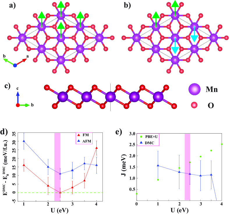
Figure 1: The top (a-b) and side (c) view of the atomic structure of monolayer MnO₂. The ferromagnetic (FM) ordering is depicted in a) while the antiferromagnetic (AFM) ordering is depicted in b) where green arrows represent spin-up and blue arrows represent spin-down. d) The DMC calculated total energies of a 36 atom supercell (normalized per formula unit (f.u.), 3 atoms) of the ferromagnetic (red) and antiferromagnetic (blue) states of 2D MnO₂ calculated as a function of the U parameter used to variationally determine the optimal trial wave function. For convenience of presentation, the DMC energies are shifted by E${}_{0}^{\textrm{DMC}}$ (the lowest DMC energy obtained for the FM ordering at U = 2.5 eV) and the green dashed line is drawn at E${}^{\textrm{DMC}}_{0}$. e) The nearest neighbor magnetic exchange parameter $J$ obtained from DMC (blue triangle) and PBE+U (green circle) calculations as a function of U value, using RRKJ pseudopotentials. Due to the fact that $J$ is negative (-1.1(7) meV) for U = 4 eV, the data point is out of the range of e). The magenta rectangle in d) - e) represents the optimal fitted U value of 2.4(1) eV.

Two dynamically stable phases, H (the trigonal prismatic phase (2H)-hexagonal honeycombs) and T (octahedral phase (1T)-centered honeycombs) of monolayer MnO₂ have been predicted stable from phonon and ab-initio molecular dynamics simulations Ataca, Şahin, and Ciraci (2012). In this work, we will focus on the T-phase of 2D MnO₂, which has been predicted to be semiconducting and magnetic, from previous studies and our own work Ataca, Şahin, and Ciraci (2012). Although the unit cell of MnO₂ can be constructed from 3 atoms (one Mn and two O), in order to study the FM and AFM states separately, larger supercells must be constructed to avoid periodic interactions of the Mn spins of the AFM state. We constructed 2x2x1 (12 atoms) and 2x1x1 (6 atoms) supercells to combat this for various DFT+U calculations. Unless otherwise noted, we normalized all of our calculated quantities to the 2x2x1 (12 atom) supercell.

The bulk counterpart of monolayer MnO₂ (in this work monolayer MnO₂ will solely refer to T-phase) is layered $\delta$-MnO₂, which is among several polymorphs of bulk MnO₂ ($\beta$, R, $\alpha$, $\gamma$, $\lambda$) Kitchaev et al. (2016). The top and side view of the atomic structure of the 2x2x1 supercell of 2D MnO₂ is given in Fig. 1 a - c), for the FM and AFM ordering. In monolayer MnO₂, each Mn atom is bonded to six O atoms in an octahedral configuration. As reported in previous literatureKan et al. (2013) and from our own spin polarized DFT calculations, the FM state has a net magnetic moment of 3 $\mu_{B}$ per unit cell arising from Mn atoms. This can be explained by the octahedral coordination, where the $d$ orbitals are split into t${}_{2\textrm{g}}$ (d_xy, d_yz, d_xz) and e${}_{\textrm{g}}^{*}$ (d${}_{z^{2}}$, d${}_{x^{2}-y^{2}}$) orbitals, where t${}_{2\textrm{g}}$ orbitals have lower energy. Since each octahedrally coordinated Mn atom has a configuration of 3d³, and the three t${}_{2\textrm{g}}$ orbitals are singly occupied with parallel spins (Hund’s rule), the unit cell has a resulting magnetic moment of 3 $\mu_{B}$.

Table 1: Benchmarking data obtained with various functionals (PBE, SCAN, LDA) and different U values using the VASP code and PAW pseudopotentials for monolayer MnO₂. For each functional/U value, the geometry of 2D MnO₂ was fully relaxed separately for the FM and AFM states (12 atom supercell, 2x2x1 of the primitive cell). The first column depicts the functionals and U value used, the second column depicts the energy differences between the optimized FM state geometry and the optimized AFM geometry, the third column depicts the optimal lattice constant of the FM state and the fourth column depicts the optimal lattice constant of the AFM state.

Functional	E${}_{\textrm{FM}}$-E${}_{\textrm{AFM}}$	FM	AFM
	(meV)	a=b (Å)	a=b (Å)
PBE, U=0	-8.2	5.772	5.749
PBE, U=2	-36.6	5.806	5.789
PBE, U=3.5	-55.0	5.838	5.817
SCAN, U=0	-3.1	5.696	5.685
SCAN, U=2	-16.0	5.723	5.712
SCAN, U=3.5	-28.7	5.754	5.735
LDA, U=0	18.0	5.636	5.615
LDA,U=2	-25.4	5.664	5.650
LDA, U=3.5	-44.1	5.685	5.671

Prior to any DMC calculations, we benchmarked the optimal geometry and energy of the FM and AFM states of monolayer MnO₂ using the VASP code (PAW potentials) with various density functionals and U corrections. The goal of these calculations was to determine whether the preferred magnetic ordering (if ground state was FM or AFM) has a strong dependence on the density functional, geometry or U correction. In Table 1, we report the energy difference between the relaxed FM and AFM configurations, and the optimal lattice constant for the FM and AFM configurations for PBE, SCAN and LDA using U values of 0, 2 and 3.5 eV (for the 2x2x1, 12 atom supercell). We chose these values of U to obtain a robust sampling of results close to (and surrounding) results previously reported in literature Kan et al. (2013); Wang, Maxisch, and Ceder (2006). The energy difference between the FM and AFM state is an important quantity because it can give insight to which magnetic state is more favorable in nature. In addition, the magnetic exchange parameters are directly calculated from the E${}_{\textrm{FM}}$-E${}_{\textrm{AFM}}$ energy.

In Table 1, we observe that the E${}_{\textrm{FM}}$-E${}_{\textrm{AFM}}$ energy is negative (FM favorable) for PBE and SCAN (U = 0, 2, 3.5 eV), LDA (U = 2.5, 3 eV), and positive (AFM favorable) for LDA (U = 0 eV). As the U value is increased, the E${}_{\textrm{FM}}$-E${}_{\textrm{AFM}}$ energy becomes more negative for each functional. In addition to the strong functional and U dependence on the E${}_{\textrm{FM}}$-E${}_{\textrm{AFM}}$ energy, there is also strong dependence on the optimal lattice constant, as seen in the last two columns of Table 1. With comparison to the experimental value of 5.69(1) Å Kitchaev et al. (2016); Chen, Zavalij, and Whittingham (1996); Pinaud et al. (2011); Ma et al. (2004) for the bulk/thin film layered $\delta$-MnO₂, the relaxed lattice constant of the FM ordered monolayer structure calculated with SCAN (U = 0 eV) is the closest to the experimental value. It is also noted that lattice constants of AFM ordering are slightly smaller than FM ordering for every functional and U values. As expected, PBE tends to overestimate the lattice constant, LDA tends to underestimate, and SCAN (meta-GGA) can achieve highly accurate lattice constants, as demonstrated in previous works Wines, Saritas, and Ataca (2020); Buda et al. (2017). For this reason, we used the fixed lattice constant and atomic positions obtained with SCAN (for FM ordering) for all subsequent DMC and DFT+U spin-orbit calculations (discussed later in this section).

Table 2: Benchmarking data obtained with various functionals (PBE, SCAN, LDA) using the VASP code and PAW pseudopotentials for monolayer MnO₂. To investigate the geometry dependence of the FM/AFM energies we took the relaxed geometries obtained with each functional and calculated the energy with a different functional (for the 12 atom supercell, 2x2x1 of the primitive cell). The first column displays which geometry was used, the second column depicts the functional used to calculate the energies, the third column depicts the energy differences between the FM state and the AFM state.

Geometry	Functional	E${}_{\textrm{FM}}$-E${}_{\textrm{AFM}}$
		(meV)
PBE	PBE	-8.2
SCAN	PBE	-4.2
LDA	PBE	-13.0
PBE	SCAN	3.1
SCAN	SCAN	-3.1
LDA	SCAN	-10.7
PBE	LDA	13.9
SCAN	LDA	11.2
LDA	LDA	18.0

To investigate further whether the E${}_{\textrm{FM}}$-E${}_{\textrm{AFM}}$ energy is functional dependent or geometry dependent, we decided to fix the FM geometry obtained with one functional, and calculate the E${}_{\textrm{FM}}$-E${}_{\textrm{AFM}}$ energy with another functional. These results are tabulated in Table 2. Here we see that regardless of the functional used to optimize the geometry, the energies for each of the three geometries are within a few meV of each other when calculated with PBE, SCAN and LDA respectively. Most evidently, LDA is predicting the AFM state to be more favorable regardless of which geometry is used. Based on the benchmarking DFT (PAW) data presented in Table 1 and Table 2, we observe that the E${}_{\textrm{FM}}$-E${}_{\textrm{AFM}}$ energy is most dependent on the functional and U parameter used and not the optimal geometry. Due to the weak dependence on geometry, we decided to use DMC to calculate the energy of the FM and AFM state of 2D MnO₂ separately, since DMC has a weak dependence on the starting wavefunction, density functional and Hubbard parameter.

As previously mentioned, we used the geometry obtained with SCAN (FM and U=0) for the subsequent DMC calculations, because the calculated lattice constant (for the 2x2x1 supercell) of 5.696 Å is identical to the experimental value of 5.69(1) Å. DMC has the zero-variance property which means that as the trial wave function approaches the exact ground state (i.e., the exact nodal surface), the statistical fluctuations in the energy reduce to zero Foulkes et al. (2001). There have been instances where various sophisticated, often times expensive methods have been used to optimize the nodal surface of the trial wave function PhysRevB.48.12037; PhysRevB.58.6800; PhysRevE.74.066701; PhysRevLett.104.193001. However, similar to other DMC studies of correlated magnetic materials Foyevtsova et al. (2014); Ichibha et al. (2021); Saritas et al. (2019a, 2018); staros, we used a PBE+U approach where the Hubbard U value was used as a variational parameter to optimize the nodal surface using DMC (for the FM and AFM states of 2D MnO₂). The fact that we can determine the optimal U parameter variationally using DMC makes our DMC results more reliable than DFT+U, where in DFT+U the U parameter is usually arbitrarily chosen or fitted to experimental data. For the case of 2D MnO₂, where experimental data for properties such as $T_{c}$ are not yet measured, the DMC determined U value can be used as a fitting parameter for subsequent DFT+U calculations. The results of these calculations (creating the nodal surface with different U values) are depicted in Fig. 1 d), where we observe an energy minimum around U = 2.5 eV for the FM and AFM states. To determine the optimal value of U, we performed a quadratic fit on the FM data depicted in Fig. 1 d) and obtained a value of U = 2.4(1) eV. We performed this fit on the FM data rather than the AFM data due to the fact that the error is smaller for the FM data and the deviation from a perfect quadratic fit is minimal (in contrast to the large deviation at U = 4 eV for the AFM data). The range of optimal U (2.4(1) eV) is depicted by the magenta rectangle in Fig. 1 d) - e) and Fig. 2 a) - b). It is important to note that energies are statistically indistinguishable for the separate FM and AFM configurations from U = 2 - 3.5 eV, demonstrating DMC’s weaker dependence on the Hubbard correction.

The full form of the model spin Hamiltonian Torelli and Olsen (2018); Lado and Fernández-Rossier (2017) is:

$${\cal{H}}=-\left(\sum_{i}D(S_{i}^{z})^{2}+\frac{J}{2}\sum_{i,i^{\prime}}\vec{S}_{i}\cdot\vec{S}_{i^{\prime}}+\frac{\lambda}{2}\sum_{i,i^{\prime}}S_{i}^{z}S_{i^{\prime}}^{z}\right)$$ (3)

where the sum over $i$ runs over the lattice of Mn atoms and $i^{\prime}$ runs over the nearest Mn site of atom $i$ due to strong magnetic moment localized on Mn atoms. Long-range interactions are shown to die out in other 2D magnetic materials Lado and Fernández-Rossier (2017), so we focused solely on the nearest neighbor interactions. The first term in the Hamiltonian describes the easy axis single ion anisotropy (with $z$ chosen as the off-plane direction). The second term is the Heisenberg isotropic exchange and the last term is the anisotropic exchange. The sign convention follows such that $J>0$ favors FM interactions, $D>0$ favors off-plane easy axis and $\lambda=0$ implies completely isotropic exchange.

First we treat Eq. 3 classically, describing the spins $\vec{S}$ collinearly as either $S=S^{x}$ or $S=S^{z}$. This makes it possible to write the energy of the ground state for 4 possible ground states: i) ferromagnetic off-plane (FM,$z$), ii) antiferromagnetic off-plane (AFM,$z$), iii) ferromagnetic in-plane (FM,$x$), and iv) antiferromagnetic in-plane (AFM,$x$). The corresponding energy equations normalized for the 2x2x1 supercell of 2D MnO₂ (4 Mn atoms) are as followed:

$$\textrm{E}_{\textrm{FM},z}=-4S^{2}D-12S^{2}(J+\lambda)$$ (4)

$$\textrm{E}_{\textrm{AFM},z}=-4S^{2}D+4S^{2}(J+\lambda)$$ (5)

$$\textrm{E}_{\textrm{FM},x}=-12S^{2}J$$ (6)

$$\textrm{E}_{\textrm{AFM},x}=+4S^{2}J$$ (7)

where $S=3/2$. We extracted the value for $J$ from our ground state energies (FM and AFM states) calculated with spin-polarized DFT+U and DMC using PBE and RRKJ pseudopotentials. In our DMC and DFT+U calculations (RRKJ), the spin on the Mn atoms is strictly up or down (spin-orbit calculations are currently not available for DMC and RRKJ pseudopotentials do not have an explicit spin-orbit contribution). This excludes us from calculating the energies from Eq. 6 and 7 using DMC and DFT+U (RRKJ) simulations due to the needed non-collinear magnetism simulations. In addition to these, only the $J+\lambda$ term can be calculated using Eq. 4 and 5 for DMC and DFT+U (RRKJ). For now, we neglect the anisotropic exchange ($\lambda$) term and calculate the magnetic exchange $J$ parameter from Eq. 4 and 5. We will clarify why $\lambda$ can be omitted for 2D MnO₂ in upcoming discussions.

Figure 1 e) depicts the nearest neighbor magnetic exchange parameter ($J$) obtained with DMC and DFT+U as a function of U value (using the PBE functional and RRKJ pseudopotentials). The $J$ parameter calculated with DFT increases linearly as U is increased, signifying the strong dependence of the Hubbard parameter on magnetic exchange at the DFT level. Despite this dependence, for all U values (including U = 0 eV), $J>0$, signifying the FM state as more energetically favorable.

On the other hand, DMC has a much weaker dependence on the U value used to create the nodal surface (from the separate FM and AFM calculations), which is indicated in Fig. 1 e), where we see the $J$ parameter is statistically identical for U = 1 - 3.5 eV. For the optimal value of U = 2.5 eV (as seen in Fig. 1 d)), we obtain a value of $J=1.2(5)$ meV. At the DMC level for U = 4 eV (not depicted in Fig. 1 e)), we observe a change from FM favorable to AFM favorable ($J=-1.1(7)$ meV), indicating that we are out of the regime where the Hubbard parameter dependence is weak (see Fig. 1 d)). Similar behavior of $J$ with respect to U has been observed in other DMC works such as in Foyevtsova et al. Foyevtsova et al. (2014).

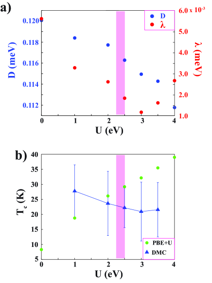
Figure 2: a) The single ion anisotropy D (blue circle) and the anisotropic exchange $\lambda$ (red circle) as a function of U, obtained from spin-orbit PBE+U calculations using PAW pseudopotentials. b) The estimated critical temperature obtained from the analytical model presented in Torelli and Olsen (2018) as a function of U, using the D and $\lambda$ results obtained from PBE+U (PAW) calculations and the $J$ results obtained from DMC (blue triangle) and PBE+U (green circle) using RRKJ pseudopotentials. The magenta rectangle in a) - b) represents the optimal fitted U value of 2.4(1) eV.

For explicit calculations of $\lambda$ and $D$, we performed self-consistent spin-orbit PBE+U calculations with PAW pseudopotentials. Specifically in these noncollinear calculations, we rotated the easy axis by 90^∘ and calculated the energy difference between the rotated and non-rotated configurations (for FM and AFM states separately). $D$ and $\lambda$ as a function of U are depicted in Fig. 2 a). We observe $D$ to be on the order of $\sim$0.1 meV and $\lambda$ to be on the order of $\sim$1 x 10^-3, which implies that the easy axis single ion anisotropy is much more dominant than the anisotropic symmetric exchange. Since magnetic anisotropy favoring vertical orientation of the spins to the layer does in fact exists for 2D MnO₂, we can confirm that FM ordering can exist in 2D for this system. In addition since $D>0$ for all values of U, the spins favor the off-plane easy axis. As seen in Fig. 2 a), changing the Hubbard parameter changes the value for $D$ and $\lambda$. $D$ tends to decrease as U is increased and $\lambda$ decreases until U = 3 eV, and then slightly increases from U = 3 - 4 eV. Due to the fact that the value of $\lambda$ is so small comparatively to $D$ and $J$, and the fact that the values of $\lambda$ for 2D MnO₂ are roughly two orders of magnitude smaller than 2D CrI₃ Lado and Fernández-Rossier (2017), we can infer that the contribution of $\lambda$ is negligible and the exchange for 2D MnO₂ is completely isotropic. In addition, this is the reason why we can safely avoid $\lambda$ for determining the $J$ parameter from DMC and DFT+U simulations (RRKJ potentials) (Eq. 4 and 5). We can also infer that the slight increase in $\lambda$ after U = 3 eV is simply an artifact of the calculation, since it is numerically difficult to determine $\lambda$ due to its small magnitude. At the value of U = 2.5 eV, the Hubbard value we obtained the optimal DMC nodal surface for, we calculated $D=0.118$ meV and $\lambda=\sim 2$ x 10^-3 meV.

From our calculations of $J$, $D$ and $\lambda$, it is possible to estimate the critical temperature using the method outlined in Torelli and Olsen Torelli and Olsen (2018). In this method, the results from classical Monte Carlo and Random Phase Approximation (RPA) simulations were used to derive a simple analytical expression for critical temperature ($T_{c}$) that depends on lattice symmetry and is a function of the exchange coupling constants ($J$, $D$, $\lambda$). Such an expression was derived to significantly simplify the theoretical search for new 2D magnetic materials with high critical temperatures. By fitting the classical simulations, an analytical function for $T_{c}$ takes the following form.

$$T_{c}=T_{c}^{\textrm{Ising}}f(x)$$ (8)

with

$$f(x)=\textrm{tanh}^{1/4}\left[\frac{6}{N_{nn}}\text{log}(1+\gamma x)\right]$$ (9)

where $\gamma=0.033$ and $N_{nn}$ is the number of nearest neighbors. $T_{c}^{\textrm{Ising}}$ is the critical temperature for the corresponding Ising model, which takes the form $T_{c}^{\textrm{Ising}}=S^{2}J\tilde{T}_{c}/k_{B}$, where $\tilde{T}_{c}$ is the fitted dimensionless critical temperature (3.64 for trigonal lattice). When single ion anisotropy and anisotropic exchange are both present, $x=\Delta/J(2S-1)$, where $\Delta$ is the spin gap that takes the form:

$$\Delta=D(2S-1)+\lambda SN_{nn}$$ (10)

Figure 2 b) depicts the critical temperature as a function of U value. The green circles represent $T_{c}$ calculated from $J$ determined with strictly PBE+U (RRKJ potentials) and $D$ and $\lambda$ determined from spin-orbit PBE+U calculations (PAW potentials). The blue triangles and corresponding error bars represent $T_{c}$ calculated from $J$ determined with DMC and also $D$ and $\lambda$ determined from spin-orbit PBE+U calculations (PAW potentials). As seen in Fig. 2 b), $T_{c}$ calculated with strictly DFT (green circles) linearly increases as a function of U, similarly to how $J$ determined with DFT increases as a function of U (see Fig.1 e)). Although the inclusion of MA decreases $T_{c}$ by $f(x)=1/5$ (see Eq. 8 - 10), the variation of $T_{c}$ (strictly DFT) with respect to U is mainly dominated by the larger changes in $J$ rather than the smaller changes in $D$ and $\lambda$ (see Fig. 2 a) and Fig. 1 e)).

In order to make a more systematic comparison between higher order methods and provide an additional benchmark, we also calculated the FM, AFM and MA energies with the screened HSE06 functional (using PAW potentials), which includes a portion of exact Fock exchange and can estimate magnetic properties with high accuracy doi:10.1063/1.1564060. With this method, we obtain a $J$ value of 1.79 meV, a $D$ value of 0.162 meV and a $\lambda$ value of $3$ x 10^-3 meV. Using these values in conjunction with the Torelli and Olsen model, we calculated a $T_{c}$ of 32.9 K. This can be directly compared to the the PBE+U (at the optimal U value of 2.5 eV) calculated $T_{c}$ value of 29.2 K, where it is in close agreement with the HSE06 obtained value (tabulated results are given in Table S1 for comparison). Determining $T_{c}$ with the $J$ extracted from DMC simulations allows us to place an upper and lower bound on the result (see Fig. 2 b)). Using the optimal nodal surface obtained with U = 2.5 eV for our DMC calculated $J$ (and subsequently the $D$ and $\lambda$ values obtained for U = 2.5 eV), we calculated a $T_{c}$ value of 22.2 $\pm$ 6.6 K. If the HSE06 calculated values for magnetic anisotropy parameters are used instead of using the $D$ and $\lambda$ from PBE+U (U = 2.5 eV), we obtain a $T_{c}$ value of 24.1 $\pm$ 6.6 K. Although this critical temperature is far below room temperature (and approximately half of the $T_{c}$ of 45 K measured for 2D CrI₃), it has been demonstrated that $T_{c}$ can be increased by applying strain Kan et al. (2013) or by placing the monolayer on a substrate Bonilla et al. (2018). To illustrate that $J$ is the driving force behind the change in $T_{c}$ (in comparison to $D$ and $\lambda$), we calculated $T_{c}$ with a fixed value of $J$ (obtained from calculations at U = 2.5 eV) and varied $D$ and $\lambda$ as a function of U, depicted in Fig. S3. From Fig. S3 we observe that $T_{c}$ remains constant for DFT and DMC for a fixed $J$ value while $D$ and $\lambda$ vary as a function of U.

As an additional theoretical benchmark, we extracted the total charge density from our DMC calculations from Eq. 1 using optimal U value from Fig. 1 d). From this extracted total charge density, we determined the spin density, ($\rho_{up}-\rho_{down}$). The inset of Fig. 3 a) depicts the spin isosurface density calculated with DMC of 2D MnO₂. Using this many-electron approach, we observe that the Mn atoms are highly spin-polarized while the O atoms are slightly polarized anti-parallel with respect to Mn atoms. To explore these properties further and benchmark with various DFT methods, we determined the spatial variations in total charge density (Fig. S4 a) - b)) and spin density (Fig. 3 a) - b)) by plotting the radial averaged densities as a function of distance for Mn and O separately. For Fig. S4 and 3, DMC is benchmarked with DFT+U (U = 0, 1, 2.5, 3.5) and RRKJ pseudopotentials are used for all calculations. Figure S4 a) depicts the total radial density for Mn. We observe that while all DFT+U results are almost indistinguishable, they significantly overestimate the density of Mn (especially around the peak at r = 0.4 Å). For O, the differences for total radial density between DMC and DFT+U is less apparent, with DMC slightly underestimating the density from r = 0 to r = 0.4 Å and slightly overestimating after r = 0.4 Å. This larger discrepancy in the Mn atom near the radial density peak (peak of $d$ orbital) is due to the fact that DFT functionals tend to unsuccessfully capture 3$d$ orbitals.

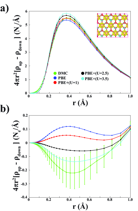
Figure 3: The spin density ($\rho_{up}-\rho_{down}$) calculated with DMC and PBE+U (U = 0, 1, 2.5, 3.5 eV) for a) Mn and b) O. The inset of a) depicts the spin isosurface density of 2D MnO₂ where the isosurface value was set to 5 x 10^-5 e/ų.

Table 3: The site-averaged atomic magnetic moments of Mn and O estimated by integrating the spin density for DMC and PBE+U results.

Method	M${}_{\textrm{Mn}}$ ($\mu_{B}$)	M${}_{\textrm{O}}$ ($\mu_{B}$)
DMC	2.77(1)	-0.10(2)
PBE, U=0	2.69	0.06
PBE, U=1	2.76	0.03
PBE, U=2.5	2.86	-0.03
PBE, U=3.5	2.93	-0.07

Although there are sizable differences for the total charge densities between PBE+U and DMC, it has been reported that various DFT methods generally give a more accurate description of spin density than the total density Kylänpää et al. (2017). Figure 3 a) depicts the radial spin density of Mn. From this figure, we observe a much closer agreement between PBE+U and DMC than for the total charge density for Mn, where the exact same shape of the curve is observed for all values of U. This demonstrates that a high quality spin density for Mn in MnO₂ can be calculated despite the different U values. In contrast to Mn, the radial spin density of O is depicted in Fig. 3 b). From our DMC result, we confirm that the O atoms are slightly polarized anti-parallel with respect to Mn atoms. From our PBE+U benchmarking, we observe that this anti-parallel polarization is completely dependent on which value of U is used. For U = 0, 1 eV the radial curve is concave up while after U = 2.5 eV, the curve is concave down, which indicates that after an effective value of U, the polarization of O atoms is corrected. These results are in accordance with our energetic results, where we determined the value of U = 2.5 eV to yield the lowest DMC energy, with U = 3.5 eV being statistically identical (see Fig. 1). We went one step further and estimated the site-averaged atomic magnetic moments per Mn and O by integrating the spin densities depicted in Fig. 3. The tabulated magnetic moments are presented in Table 3, where the results match the trends depicted in Fig. 3. In contrast to the values presented in Table 3, HSE06 (PAW) predicts a magnetic moment of 2.97 $\mu_{B}$ for Mn and -0.02 $\mu_{B}$ for O, indicating that the HSE06 Mn magnetic moment is closest to PBE+U = 3.5 and the HSE06 O magnetic moment is closest to PBE+U = 2.5. By integrating the spin densities, we have a clear picture of how the magnetization of each ion changes with respect to the electronic structure method used. Our total charge density and spin density results and magnetic moment estimates serve as an ultimate many-body theoretical benchmark for the magnetic properties of 2D MnO₂ and give insight on how to assess the accuracy of DFT calculations when various values of U are employed.

IV Conclusion

To resolve the discrepancies that arise in DFT calculations that have a strong dependence on density functional and Hubbard parameter (U), we employed DMC to calculate the energetic and magnetic properties of monolayer MnO₂. From these calculations, we found that the FM phase is more energetically favorable than the AFM phase and found the optimal U value that yields the lowest total energy to be 2.4(1) eV. By taking the difference of the FM and AFM energies calculated with DMC, we were able to estimate a Heisenberg isotropic exchange parameter ($J$) of 1.2(5) meV at the optimal U value. Using spin-orbit DFT+U (PAW method), we calculated the single ion anisotropy ($D$) and the anisotropic symmetric exchange ($\lambda$). By combining the DMC results for $J$ and DFT+U results for $D$ and $\lambda$ obtained at U = 2.4(1), we estimated the upper bound on $T_{c}$ to be 28.8 K. Additionally, we extracted the spin-density isosurfaces and the radial averaged spin density for Mn and O atoms separately from our DMC results and provide a detailed comparison with DFT+U. Our findings demonstrate the success of DMC being applied to a 2D magnetic system and provide an ultimate theoretical benchmark that will aid in guiding experimentalists in synthesizing and characterizing 2D magnets.

References

References

- Huang et al. (2017) B. Huang, G. Clark, E. Navarro-Moratalla, D. R. Klein, R. Cheng, K. L. Seyler, D. Zhong, E. Schmidgall, M. A. McGuire, D. H. Cobden, W. Yao, D. Xiao, P. Jarillo-Herrero, and X. Xu, “Layer-dependent ferromagnetism in a van der waals crystal down to the monolayer limit,” Nature 546, 270–273 (2017).
- Gong et al. (2017) C. Gong, L. Li, Z. Li, H. Ji, A. Stern, Y. Xia, T. Cao, W. Bao, C. Wang, Y. Wang, Z. Q. Qiu, R. J. Cava, S. G. Louie, J. Xia, and X. Zhang, “Discovery of intrinsic ferromagnetism in two-dimensional van der Waals crystals,” Nature 546, 265–269 (2017).
- Bonilla et al. (2018) M. Bonilla, S. Kolekar, Y. Ma, H. C. Diaz, V. Kalappattil, R. Das, T. Eggers, H. R. Gutierrez, M.-H. Phan, and M. Batzill, “Strong room-temperature ferromagnetism in VSe2 monolayers on van der Waals substrates,” Nature Nanotechnology 13, 289–293 (2018).
- Sachs et al. (2013) B. Sachs, T. O. Wehling, K. S. Novoselov, A. I. Lichtenstein, and M. I. Katsnelson, “Ferromagnetic two-dimensional crystals: Single layers of K2CuF4,” Phys. Rev. B 88, 201402 (2013).
- Chittari et al. (2016) B. L. Chittari, Y. Park, D. Lee, M. Han, A. H. MacDonald, E. Hwang, and J. Jung, “Electronic and magnetic properties of single-layer metal phosphorous trichalcogenides,” Phys. Rev. B 94, 184428 (2016).
- Sarikurt et al. (2018) S. Sarikurt, Y. Kadioglu, F. Ersan, E. Vatansever, O. U. Akturk, Y. Yuksel, U. Akinci, and E. Akturk, “Electronic and magnetic properties of monolayer -RuCl3: a first-principles and Monte Carlo study,” Phys. Chem. Chem. Phys. 20, 997–1004 (2018).
- Ersan et al. (2019) F. Ersan, E. Vatansever, S. Sarikurt, Y. Yuksel, Y. Kadioglu, H. D. Ozaydin, O. U. Akturk, U. Akinci, and E. Akturk, “Exploring the electronic and magnetic properties of new metal halides from bulk to two-dimensional monolayer: RuX3 (X = Br, I),” Journal of Magnetism and Magnetic Materials 476, 111–119 (2019).
- Omomo et al. (2003) Y. Omomo, T. Sasaki, Wang, and M. Watanabe, “Redoxable nanosheet crystallites of MnO2 derived via delamination of a layered manganese oxide,” Journal of the American Chemical Society, Journal of the American Chemical Society 125, 3568–3575 (2003).
- Kitchaev et al. (2016) D. A. Kitchaev, H. Peng, Y. Liu, J. Sun, J. P. Perdew, and G. Ceder, “Energetics of polymorphs in density functional theory,” Phys. Rev. B 93, 045132 (2016).
- Rong, Zhang, and Liu (2019) S. Rong, P. Zhang, and F. Liu, “Scalable synthesis of water-dispersible 2D manganese dioxide monosheets,” Journal of Physics: Condensed Matter 32, 015301 (2019).
- Sakai et al. (2005) N. Sakai, Y. Ebina, K. Takada, and T. Sasaki, “Photocurrent generation from semiconducting manganese oxide nanosheets in response to visible light,” The Journal of Physical Chemistry B 109, 9651–9655 (2005).
- Sun et al. (2011) C. Sun, Y. Wang, J. Zou, and S. C. Smith, “A formation mechanism of oxygen vacancies in a MnO2 monolayer: a DFT + U study,” Phys. Chem. Chem. Phys. 13, 11325–11328 (2011).
- Liu et al. (2016) H.-J. Liu, J.-C. Lin, Y.-W. Fang, J.-C. Wang, B.-C. Huang, X. Gao, R. Huang, P. R. Dean, P. D. Hatton, Y.-Y. Chin, H.-J. Lin, C.-T. Chen, Y. Ikuhara, Y.-P. Chiu, C.-S. Chang, C.-G. Duan, Q. He, and Y.-H. Chu, “A metal–insulator transition of the buried MnO2 monolayer in complex oxide heterostructure,” Advanced Materials 28, 9142–9151 (2016).
- Ataca, Şahin, and Ciraci (2012) C. Ataca, H. Şahin, and S. Ciraci, “Stable, single-layer MX2 transition-metal oxides and dichalcogenides in a honeycomb-like structure,” The Journal of Physical Chemistry C 116, 8983–8999 (2012).
- Kan et al. (2013) M. Kan, J. Zhou, Q. Sun, Y. Kawazoe, and P. Jena, “The intrinsic ferromagnetism in a MnO2 monolayer,” The Journal of Physical Chemistry Letters 4, 3382–3386 (2013).
- Wang, Maxisch, and Ceder (2006) L. Wang, T. Maxisch, and G. Ceder, “Oxidation energies of transition metal oxides within the framework,” Phys. Rev. B 73, 195107 (2006).
- Mermin and Wagner (1966) N. D. Mermin and H. Wagner, “Absence of ferromagnetism or antiferromagnetism in one- or two-dimensional isotropic heisenberg models,” Phys. Rev. Lett. 17, 1133–1136 (1966).
- Torelli and Olsen (2018) D. Torelli and T. Olsen, “Calculating critical temperatures for ferromagnetic order in two-dimensional materials,” 2D Materials 6, 015028 (2018).
- Foulkes et al. (2001) W. M. C. Foulkes, L. Mitas, R. J. Needs, and G. Rajagopal, “Quantum Monte Carlo simulations of solids,” Rev. Mod. Phys. 73, 33–83 (2001).
- Hao et al. (2018) H. Hao, J. Shee, S. Upadhyay, C. Ataca, K. D. Jordan, and B. M. Rubenstein, “Accurate predictions of electron binding energies of dipole-bound anions via Quantum Monte Carlo methods,” The Journal of Physical Chemistry Letters 9, 6185–6190 (2018).
- Szyniszewski et al. (2017) M. Szyniszewski, E. Mostaani, N. D. Drummond, and V. I. Fal’ko, “Binding energies of trions and biexcitons in two-dimensional semiconductors from Diffusion Quantum Monte Carlo calculations,” Phys. Rev. B 95, 081301 (2017).
- Mostaani et al. (2017) E. Mostaani, M. Szyniszewski, C. H. Price, R. Maezono, M. Danovich, R. J. Hunt, N. D. Drummond, and V. I. Fal’ko, “Diffusion Quantum Monte Carlo study of excitonic complexes in two-dimensional transition-metal dichalcogenides,” Phys. Rev. B 96, 075431 (2017).
- Saritas et al. (2019a) K. Saritas, J. T. Krogel, S. Okamoto, H. N. Lee, and F. A. Reboredo, “Structural, electronic, and magnetic properties of bulk and epitaxial through Diffusion Monte Carlo,” Phys. Rev. Materials 3, 124414 (2019a).
- Luo et al. (2016) Y. Luo, A. Benali, L. Shulenburger, J. T. Krogel, O. Heinonen, and P. R. C. Kent, “Phase stability of TiO2 polymorphs from Diffusion Quantum Monte Carlo,” New Journal of Physics 18, 113049 (2016).
- Benali et al. (2016) A. Benali, L. Shulenburger, J. T. Krogel, X. Zhong, P. R. C. Kent, and O. Heinonen, “Quantum Monte Carlo analysis of a charge ordered insulating antiferromagnet: the Ti4O7 Magnéli phase,” Phys. Chem. Chem. Phys. 18, 18323–18335 (2016).
- Santana et al. (2015) J. A. Santana, J. T. Krogel, J. Kim, P. R. C. Kent, and F. A. Reboredo, “Structural stability and defect energetics of ZnO from Diffusion quantum Monte Carlo,” The Journal of Chemical Physics 142, 164705 (2015).
- Saritas, Krogel, and Reboredo (2018) K. Saritas, J. T. Krogel, and F. A. Reboredo, “Relative energies and electronic structures of CoO polymorphs through ab initio Diffusion Quantum Monte Carlo,” Phys. Rev. B 98, 155130 (2018).
- Wang, Annaberdiyev, and Mitas (2020) G. Wang, A. Annaberdiyev, and L. Mitas, “Binding and excitations in SixHy molecular systems using Quantum Monte Carlo,” The Journal of Chemical Physics 153, 144303 (2020).
- Bennett et al. (2021) M. C. Bennett, G. Hu, G. Wang, O. Heinonen, P. R. C. Kent, J. T. Krogel, and P. Ganesh, “Origin of metal-insulator transitions in correlated perovskite metals,” (2021), arXiv:2103.09809 [cond-mat.mtrl-sci] .
- Annaberdiyev et al. (2021) A. Annaberdiyev, G. Wang, C. A. Melton, M. C. Bennett, and L. Mitas, “Cohesion and excitations of diamond-structure silicon by quantum Monte Carlo: Benchmarks and control of systematic biases,” Phys. Rev. B 103, 205206 (2021).
- Foyevtsova et al. (2014) K. Foyevtsova, J. T. Krogel, J. Kim, P. R. C. Kent, E. Dagotto, and F. A. Reboredo, “Ab initio Quantum Monte Carlo calculations of spin superexchange in cuprates: The benchmarking case of ,” Phys. Rev. X 4, 031003 (2014).
- Busemeyer et al. (2016) B. Busemeyer, M. Dagrada, S. Sorella, M. Casula, and L. K. Wagner, “Competing collinear magnetic structures in superconducting FeSe by first-principles quantum Monte Carlo calculations,” Phys. Rev. B 94, 035108 (2016).
- Saritas et al. (2018) K. Saritas, J. T. Krogel, P. R. C. Kent, and F. A. Reboredo, “Diffusion monte carlo: A pathway towards an accurate theoretical description of manganese oxides,” Phys. Rev. Materials 2, 085801 (2018).
- Shin et al. (2021) H. Shin, J. T. Krogel, K. Gasperich, P. R. C. Kent, A. Benali, and O. Heinonen, “Optimized structure and electronic band gap of monolayer GeSe from Quantum Monte Carlo methods,” Phys. Rev. Materials 5, 024002 (2021).
- Wines, Saritas, and Ataca (2020) D. Wines, K. Saritas, and C. Ataca, “A first-principles Quantum Monte Carlo study of two-dimensional (2D) GaSe,” The Journal of Chemical Physics 153, 154704 (2020).
- Wines, Saritas, and Ataca (2021) D. Wines, K. Saritas, and C. Ataca, “A pathway toward high-throughput quantum Monte Carlo simulations for alloys: A case study of two-dimensional (2d) GaSxSe1-x,” The Journal of Chemical Physics 155, 194112 (2021).
- Shulenburger et al. (2015) L. Shulenburger, A. D. Baczewski, Z. Zhu, J. Guan, and D. Tománek, “The nature of the interlayer interaction in bulk and few-layer phosphorus,” Nano Letters 15, 8170–8175 (2015).
- Frank et al. (2019) T. Frank, R. Derian, K. Tokár, L. Mitas, J. Fabian, and I. Štich, “Many-body Quantum Monte Carlo study of 2D materials: Cohesion and band gap in single-layer phosphorene,” Phys. Rev. X 9, 011018 (2019).
- Mostaani, Drummond, and Fal’ko (2015) E. Mostaani, N. D. Drummond, and V. I. Fal’ko, “Quantum Monte Carlo calculation of the binding energy of bilayer graphene,” Phys. Rev. Lett. 115, 115501 (2015).
- Kadioglu et al. (2018) Y. Kadioglu, J. A. Santana, H. D. Ozaydin, F. Ersan, O. U. Akturk, E. Akturk, and F. A. Reboredo, “Diffusion Quantum Monte Carlo and density functional calculations of the structural stability of bilayer arsenene,” The Journal of Chemical Physics 148, 214706 (2018).
- Saritas et al. (2019b) K. Saritas, W. Ming, M.-H. Du, and F. A. Reboredo, “Excitation energies of localized correlated defects via Quantum Monte Carlo: A case study of Mn4+-doped phosphors,” The Journal of Physical Chemistry Letters 10, 67–74 (2019b).
- Kylänpää et al. (2017) I. Kylänpää, J. Balachandran, P. Ganesh, O. Heinonen, P. R. C. Kent, and J. T. Krogel, “Accuracy of ab initio electron correlation and electron densities in vanadium dioxide,” Phys. Rev. Materials 1, 065408 (2017).
- Kresse and Furthmüller (1996) G. Kresse and J. Furthmüller, “Efficient iterative schemes for ab initio total-energy calculations using a plane-wave basis set,” Phys. Rev. B 54, 11169–11186 (1996).
- Kresse and Joubert (1999) G. Kresse and D. Joubert, “From ultrasoft pseudopotentials to the projector augmented-wave method,” Phys. Rev. B 59, 1758–1775 (1999).
- Perdew, Burke, and Ernzerhof (1996) J. P. Perdew, K. Burke, and M. Ernzerhof, “Generalized gradient approximation made simple,” Phys. Rev. Lett. 77, 3865–3868 (1996).
- Hohenberg and Kohn (1964) P. Hohenberg and W. Kohn, “Inhomogeneous electron gas,” Phys. Rev. 136, B864–B871 (1964).
- Sun, Ruzsinszky, and Perdew (2015) J. Sun, A. Ruzsinszky, and J. P. Perdew, “Strongly constrained and appropriately normed semilocal density functional,” Phys. Rev. Lett. 115, 036402 (2015).
- Dudarev et al. (1998) S. L. Dudarev, G. A. Botton, S. Y. Savrasov, C. J. Humphreys, and A. P. Sutton, “Electron-energy-loss spectra and the structural stability of nickel oxide: An LSDA+U study,” Phys. Rev. B 57, 1505–1509 (1998).
- Giannozzi et al. (2009) P. Giannozzi, S. Baroni, N. Bonini, M. Calandra, R. Car, C. Cavazzoni, D. Ceresoli, G. L. Chiarotti, M. Cococcioni, I. Dabo, A. D. Corso, S. de Gironcoli, S. Fabris, G. Fratesi, R. Gebauer, U. Gerstmann, C. Gougoussis, A. Kokalj, M. Lazzeri, L. Martin-Samos, N. Marzari, F. Mauri, R. Mazzarello, S. Paolini, A. Pasquarello, L. Paulatto, C. Sbraccia, S. Scandolo, G. Sclauzero, A. P. Seitsonen, A. Smogunov, P. Umari, and R. M. Wentzcovitch, “QUANTUM ESPRESSO: a modular and open-source software project for quantum simulations of materials,” Journal of Physics: Condensed Matter 21, 395502 (2009).
- Krogel, Santana, and Reboredo (2016) J. T. Krogel, J. A. Santana, and F. A. Reboredo, “Pseudopotentials for quantum Monte Carlo studies of transition metal oxides,” Phys. Rev. B 93, 075143 (2016).
- Needs et al. (2009) R. J. Needs, M. D. Towler, N. D. Drummond, and P. L. Ríos, “Continuum Variational and Diffusion Quantum Monte Carlo calculations,” Journal of Physics: Condensed Matter 22, 023201 (2009).
- Kim et al. (2018) J. Kim, A. D. Baczewski, T. D. Beaudet, A. Benali, M. C. Bennett, M. A. Berrill, N. S. Blunt, E. J. L. Borda, M. Casula, D. M. Ceperley, S. Chiesa, B. K. Clark, R. C. Clay, K. T. Delaney, M. Dewing, K. P. Esler, H. Hao, O. Heinonen, P. R. C. Kent, J. T. Krogel, I. Kylänpää, Y. W. Li, M. G. Lopez, Y. Luo, F. D. Malone, R. M. Martin, A. Mathuriya, J. McMinis, C. A. Melton, L. Mitas, M. A. Morales, E. Neuscamman, W. D. Parker, S. D. P. Flores, N. A. Romero, B. M. Rubenstein, J. A. R. Shea, H. Shin, L. Shulenburger, A. F. Tillack, J. P. Townsend, N. M. Tubman, B. V. D. Goetz, J. E. Vincent, D. C. Yang, Y. Yang, S. Zhang, and L. Zhao, “QMCPACK: an open source ab initio quantum Monte Carlo package for the electronic structure of atoms, molecules and solids,” Journal of Physics: Condensed Matter 30, 195901 (2018).
- Kent et al. (2020) P. R. C. Kent, A. Annaberdiyev, A. Benali, M. C. Bennett, E. J. Landinez Borda, P. Doak, H. Hao, K. D. Jordan, J. T. Krogel, I. Kylänpää, J. Lee, Y. Luo, F. D. Malone, C. A. Melton, L. Mitas, M. A. Morales, E. Neuscamman, F. A. Reboredo, B. Rubenstein, K. Saritas, S. Upadhyay, G. Wang, S. Zhang, and L. Zhao, “QMCPACK: Advances in the development, efficiency, and application of auxiliary field and real-space Variational and Diffusion Quantum Monte Carlo,” The Journal of Chemical Physics 152, 174105 (2020).
- Slater (1929) J. C. Slater, “The theory of complex spectra,” Phys. Rev. 34, 1293–1322 (1929).
- Jastrow (1955) R. Jastrow, “Many-body problem with strong forces,” Phys. Rev. 98, 1479–1484 (1955).
- Umrigar and Filippi (2005) C. J. Umrigar and C. Filippi, “Energy and variance optimization of many-body wave functions,” Phys. Rev. Lett. 94, 150201 (2005).
- Mitas, Shirley, and Ceperley (1991) L. Mitas, E. L. Shirley, and D. M. Ceperley, “Nonlocal pseudopotentials and Diffusion Monte Carlo,” The Journal of Chemical Physics 95, 3467–3475 (1991).
- Drummond, Towler, and Needs (2004) N. D. Drummond, M. D. Towler, and R. J. Needs, “Jastrow correlation factor for atoms, molecules, and solids,” Phys. Rev. B 70, 235119 (2004).
- Umrigar et al. (2007) C. J. Umrigar, J. Toulouse, C. Filippi, S. Sorella, and R. G. Hennig, “Alleviation of the fermion-sign problem by optimization of many-body wave functions,” Phys. Rev. Lett. 98, 110201 (2007).
- Krogel (2016) J. T. Krogel, “Nexus: A modular workflow management system for quantum simulation codes,” Computer Physics Communications 198, 154 – 168 (2016).
- Lado and Fernández-Rossier (2017) J. L. Lado and J. Fernández-Rossier, “On the origin of magnetic anisotropy in two dimensional CrI3,” 2D Materials 4, 035002 (2017).
- Chen, Zavalij, and Whittingham (1996) R. Chen, P. Zavalij, and M. S. Whittingham, “Hydrothermal synthesis and characterization of KxMnO2·yH2O,” Chemistry of Materials 8, 1275–1280 (1996).
- Pinaud et al. (2011) B. A. Pinaud, Z. Chen, D. N. Abram, and T. F. Jaramillo, “Thin films of sodium birnessite-type MnO2: Optical properties, electronic band structure, and solar photoelectrochemistry,” The Journal of Physical Chemistry C 115, 11830–11838 (2011).
- Ma et al. (2004) R. Ma, Y. Bando, L. Zhang, and T. Sasaki, “Layered MnO2 nanobelts: Hydrothermal synthesis and electrochemical measurements,” Advanced Materials 16, 918–922 (2004).
- Buda et al. (2017) I. G. Buda, C. Lane, B. Barbiellini, A. Ruzsinszky, J. Sun, and A. Bansil, “Characterization of thin film materials using SCAN meta-GGA, an accurate nonempirical density functional,” Scientific Reports 7, 44766 (2017).
- Ichibha et al. (2021) T. Ichibha, A. L. Dzubak, J. T. Krogel, V. R. Cooper, and F. A. Reboredo, “ revisited with a many-body ab initio theoretical approach,” Phys. Rev. Materials 5, 064006 (2021).