XMM-Newton detection of soft time lags in the TDE candidate AT 2018fyk

Abstract

In this letter we report a tentative detection of soft time lags (i.e. variability of softer photons lags behind the variability of harder photons) in one XMM-Newton observation of the tidal disruption event (TDE) candidate AT 2018fyk while the source was in the hard spectral state. The lags are detected at $6.51\times 10^{-5}~{}\rm Hz$. The amplitude of the lags with respect to 0.5$-$1 keV monotonically decreases with the photon energy, from $\sim 1200~{}\rm s$ at 0.3$-$0.5 keV to $\sim-4200~{}\rm s$ at 3$-$5 keV (in our convention a positive lag means lagging behind the reference band). We find that the amplitude is proportional to the logarithm of the energy separation between the examined band and the reference band. The energy-dependent covariance spectrum indicates that the correlated variability is more likely to be associated with the non-thermal radiation. The soft lags are difficult to reconcile with the reverberation scenario that are used to explain the soft lags in active galactic nuclei. On the other hand, the observed soft lags are consistent with the picture that the soft X-rays are down-scattered hard X-rays by the outflow as predicted by “unification” models of TDEs.

1 Introduction

Tidal disruption events (TDEs) are transient events caused by super-massive black holes (SMBHs) tidally disrupting nearby stars and accreting stellar debris (see Gezari, 2021, for a review). TDEs offer us unique opportunities to study dormant SMBHs. So far, a few tens of TDEs have been discovered. Depending on their X-ray properties, TDEs can be classified into two categories: X-ray TDEs that are detected in X-rays, and optical-UV TDEs that lack X-ray emission. Understanding the X-ray/optical-UV dichotomy is an important task in the study of TDEs.

To explain the weak X-ray emission of optical-UV TDEs, several models have been proposed. The first set of models (often referred to as “unification” models of TDEs) claimed that the dichotomy is a viewing angle effect: the X-ray and optical-UV TDEs are intrinsically the same, but for observers at large inclinations the X-ray radiation is obscured by the wind launched by the super-Eddington accretion disc (e.g. Dai et al., 2018). In the second set of models, the dichotomy is intrinsic; the strength of the X-ray emission depends on the physical properties of the system. For instance, it has been proposed that the disc formation is faster for TDEs with larger black hole mass (e.g. Guillochon & Ramirez-Ruiz, 2015), resulting in the absence of X-ray emission in the early outburst stage of low-mass TDEs.

AT 2018fyk is a candidate X-ray TDE discovered by the ASAS-SN on September 8th, 2018 (Stanek, 2018). It is located at the nucleus of LCRS B224721.6$-$450748, a galaxy at a redshift of 0.06. Wevers (2020) measured the mass of the central SMBH of the galaxy using the $M-\sigma$ relation, and found ${\rm log_{10}}\ M_{\rm BH}=7.7\pm 0.4$ where $M_{\rm BH}$ is the black hole mass in solar mass. Wevers et al. (2019) performed a multi-wavelength study of AT 2018fyk and found evidences for rapid disc formation. Wevers et al. (2021) studied the long-term evolution of the X-ray emission of AT 2018fyk, and discovered an X-ray state transition of AT 2018fyk from a soft, thermal-dominated spectral state to a hard, non-thermal dominated state. The spectral state transition is accompanied by a change in the timing properties, with high-frequency variability ($\gtrsim 10^{-5}~{}\rm Hz$) emerging after the state transition.

We perform Fourier time-lag analysis of AT 2018fyk. Fourier time-lag analysis has been proved to be a great tool to study the accretion flow around black holes with mass across a large dynamic range. Time-lag analysis of both active galactic nuclei (AGNs) and black hole X-ray binaries (BHXRBs) has revealed continuum hard lags (e.g. Papadakis et al., 2001; McHardy et al., 2004; Arévalo et al., 2006; Arévalo et al., 2008; Sriram et al., 2009; Epitropakis & Papadakis, 2017; Papadakis et al., 2019; Miyamoto et al., 1988; Miyamoto & Kitamoto, 1989; Nowak & Vaughan, 1996; Nowak et al., 1999; Cui et al., 2000; Crary et al., 1998; Reig et al., 2003; Altamirano & Méndez, 2015). On top of the continuum hard lags, there have been detections of soft lags where the variability of softer bands are lagging behind the harder bands. The soft lags were first detected by Fabian et al. (2009) in 1H 0707$-$495, and then in other AGNs (e.g. Zoghbi & Fabian, 2011; Cackett et al., 2013; Fabian et al., 2013; De Marco et al., 2013a; Alston et al., 2014), as well as in BHXRBs (e.g. Uttley et al., 2011; De Marco et al., 2015; De Marco et al., 2017). The soft lags are believed to be the lags between the hard coronal emission and the reflection emission due to the hard coronal emission irradiating the disc, and are consequently referred to as “reverberation lags”. De Marco et al. (2013a) performed a systematic study of the reverberation lags, and found correlations between the amplitude of the reverberation lags and the black hole mass, and between the variability frequency and the black hole mass.

Soft lags have been detected in ultra-luminous X-ray sources (ULXs) as well (Heil & Vaughan, 2010; De Marco et al., 2013b; Hernández-García et al., 2015; Pinto et al., 2017; Kara et al., 2020; Pintore et al., 2021; Mondal et al., 2021). ULXs are extragalactic, off-nuclear, ultra-luminous ($\gtrsim 10^{39}~{}\rm erg~{}s^{-1}$) X-ray sources. It is generally believed that the majority of ULXs are stellar-mass black holes or neutron stars accreting at super-Eddington rates, instead of intermediate-mass black holes (IMBHs) accreting at sub-Eddington rates. Most of the soft lags in ULXs have amplitudes of a few hundreds to thousands of seconds and are usually interpreted as the time lags due to hard X-ray photons getting down-scattered by the outflow.

In this letter we report a detection of soft lags in AT 2018fyk. The letter is organised as follows. The procedure of data reduction is illustrated in Sec. 2. The results are presented in Sec. 3. We discuss the results in Sec. 4.

2 Data Reduction

XMM-Newton observed AT 2018fyk three times. The source was detected in the first (obs id: 0831790201) and second (obs id: 0853980201) observations, and undetected in the last observation. During the first observation AT 2018fyk was in the soft state, and no X-ray variability was detected above $\sim 10^{-5}~{}\rm Hz$, while during the second observation strong high-frequency ($\gtrsim 10^{-5}~{}\rm Hz$) X-ray variability was discovered (Wevers et al., 2021). We therefore perform Fourier time-lag analysis on the pn data of 0853980201.

The observation 0853980201 were taken on Oct. 27th, 2019. During the observation pn was operating in the full-frame mode. The data are reduced with the the XMM-Newton science analysis system (SAS) version 18 following standard procedures. We produce the pn clean event list with epproc. We filter the event list to remove periods contaminated by high particle background flares, where the good time interval is defined to be the period during which the 10$-$12 keV count rate is no larger than $0.4~{}\rm counts/s$. We are left with a $\sim 30~{}\rm ks$ exposure after removing flaring backgrounds. The source and background lightcurves are extracted from the filtered event list with evselect. When extracting the lightcurves we select single and double events ($PATTERN\leq 4$) with $FLAG==0$. The source region is a circle centering on the source position with a radius of 35”. The background lightcurves are extracted from a source-free region close to the source with the same radius. The source lightcurves are then corrected for background and various other effects using epiclccorr. We also extract source and background spectra with evselect, and generate corresponding ancillary file and redistribution matrix using arfgen and rmfgen, respectively.

We extract 30-s lightcurves of 5 energy bands: $0.3-0.5~{}\rm keV$, $0.5-1~{}\rm keV$, $1-2~{}\rm keV$, $2-3~{}\rm keV$, and $3-5~{}\rm keV$. Above $\sim 5$ keV the background is stronger than the source so we exclude the $>5~{}\rm keV$ bands in our analysis. For each energy band we split the lightcurve into 2 segments, each $\sim 15~{}\rm ks$ long. Taking $0.5-1~{}\rm keV$ as the reference, we follow Epitropakis & Papadakis (2016) to compute the frequency-dependent Fourier time lags. We estimate the significance and uncertainty of the time-lag measurements by performing Monte$-$Carlo simulations. Detailed procedures of the simulations can be found in the Appendix.

3 Results

3.1 Time-lag analysis

The frequency-resolved time lags and the coherence are presented in the upper and lower panels of Fig. 1, respectively. Note that in our convention a positive lag means lagging behind the reference band. The coherence is close to unity at the lowest frequency $6.51\times 10^{-5}~{}\rm Hz$, decreases with the frequency, and drops to zero above $\sim 2\times 10^{-3}~{}\rm Hz$.

The time lags are close to zero except at $6.51\times 10^{-5}~{}\rm Hz$, the lowest frequency we can reach. At $6.51\times 10^{-5}~{}\rm Hz$, the confidence levels of the time-lags are $92.0\%$, $97.5\%$, $97.9\%$, and $97.9\%$, for 0.3$-$0.5 keV, 1$-$2 keV, 2$-$3 keV, and 3$-$5 keV, respectively. The maximum confidence level of $97.9\%$ corresponds to a significance of $\sim 1.8\sigma$. The most surprising result is that the time lags are soft, i.e. variability of soft photons are lagging behind variability of hard photons. This is opposite to AGNs where the continuum time lags are hard (e.g. Arévalo et al., 2006; Arévalo et al., 2008; Sriram et al., 2009; Epitropakis & Papadakis, 2017). The amplitude of the time lags monotonically decreases with the energy, from $1200~{}\rm s$ at the 0.3$-$0.5 keV band to $-4200~{}\rm s$ at the 3$-$5 keV band.

In Fig. 2 we plot the amplitude of the time lags at $6.51\times 10^{-5}~{}\rm Hz$ as a function of the centroid energy of the energy bands. The data points seem to fall on a straight line on the plot where the time lags and energy are plotted in linear and logarithmic scales, respectively. This implies that the time lags depend logarithmically on the energy separation between two energy bands. We fit the data with a logarithmic model, and find:

$$\tau=(-5.63\pm 0.80)\times 10^{3}\ {\rm log_{10}}\left(\frac{E_{2}}{E_{1}}\right)~{}\rm s,$$ (1)

where $\tau$ is the amplitude of the time lag, and $E_{1}$, $E_{2}$ are the centroid energies of the two energy bands. The best-fit model is plotted in a dashed line in Fig. 2. By comparing the data and the model, it is obvious that the model fits the data well, confirming the logarithmic dependence.

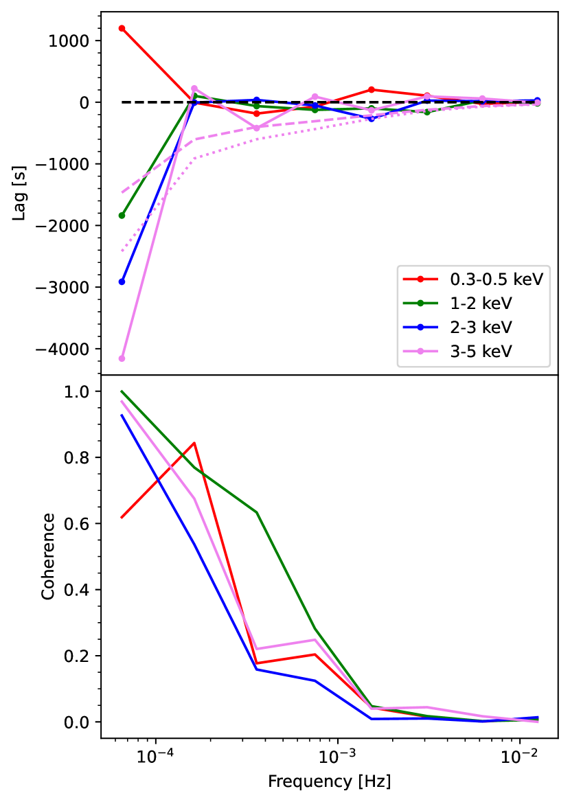
Figure 1: The Fourier time lags (upper panel) with respect to $0.5-1~{}\rm keV$ and the coherence (lower panel). The results of different energy bands are plotted in different colors, as indicated in the plot. In our convention a positive lag means lagging behind the reference band. For $3-5~{}\rm keV$, the 90% and 95% confidence levels are plotted in dashed and dotted lines, respectively.

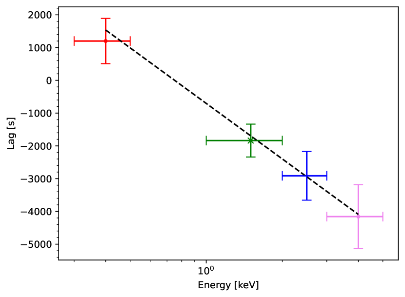
Figure 2: The time lags at $6.51\times 10^{-5}~{}\rm Hz$ as a function of the central energy of the energy bands. The error bars correspond to 68% uncertainty. We fit the lag-energy data with a logarithmic function and the best-fit model is shown by the black dashed line.

3.2 Energy and covariance spectrum

We fit the pn energy spectrum with Xspec 12.11.1. The spectrum is rebinned with specgroup to ensure minimum counts of 30 per bin. We fit the model to the data using the $\chi^{2}$ statistics. We fit the pn spectrum with the following spectral model: $phabs*(blackbody+powerlaw)$, which includes two components: a thermal blackbody component, and a nonthermal powerlaw component, both of which are absorbed by interstellar media. The spectrum and best-fit model are plotted in Fig. 3. The best-fit model (black solid) yields $\chi^{2}_{\nu}=1.47$ (with 83 degrees of freedom), and consists of a dominating powerlaw component (black dashed) with $\Gamma=2.32^{+0.09}_{-0.07}$ and a soft thermal component (black dotted) with a temperature of $100^{+7}_{-4}~{}\rm eV$.

To investigate the origin of the correlated variability, we also calculate the covariance spectrum in the frequency range of $3.7\times 10^{-5}-1.7\times 10^{-4}~{}\rm Hz$. We extract lightcurves with time resolution of $3000~{}\rm s$, and split the lightcurves into 2 segments, each of which contains 9 bins. Then we compute the covariance spectrum and its uncertainty following (Wilkinson & Uttley, 2009), taking the 0.5$-$1 keV band as the reference. The covariance spectrum is plotted in blue in Fig. 3. The shape of the covariance spectrum indicates that the correlated variability is more likely to be associated with the non-thermal emission than the thermal emission.

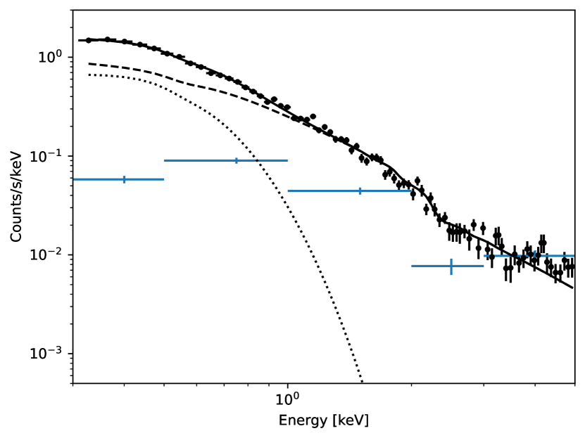
Figure 3: The covariance spectrum in blue colors. We also plot the energy spectra (black dots), the best-fit model (black solid), and the two components of the model: blackbody (black dotted) and powerlaw (black dashed).

4 Discussion and Conclusions

We tentatively detect soft time lags in one XMM-Newton observation of the TDE candidate AT 2018fyk. The observation (obs id: 0853980201) was taken while the source was in the hard spectral state. The lags are detected at $6.51\times 10^{-5}~{}\rm Hz$, and the amplitude of the lags with respect to the 0.5$-$1 keV reference band are proportional to the logarithm of the energy separation between the examined band and the reference band, ranging from $1200$ to $-4200$ seconds. The time-lags of 2$-$3 keV and 3$-$5 keV are most significant, both with a confidence level of $97.9\%$.

A model fit confirms the apparent logarithmic dependence. The coherence is close to unity at $6.51\times 10^{-5}~{}\rm Hz$ and drops rapidly with the variability frequency.

We extract the energy spectrum and fit it with a two-component model. The best-fit model consists of a thermal component with a temperature of $\sim 100~{}\rm eV$ and a dominating non-thermal component with a photon index of $\sim 2$. We also calculate the energy-dependent covariance spectrum. The shape of the covariance spectrum indicates that the correlated variability is associated with the non-thermal emission.

Below we discuss possible physical origins of the soft lags.

4.1 Reverberation lag

It is well established that the soft lags in AGNs are “reverberation lags”, i.e. the time lags between the primary hard X-ray radiation emitted by hot coronae, and the reflection radiation of the accretion disc due to primary radiation irradiating the disc. De Marco et al. (2013a) performed a systematic study of the reverberation lags in AGNs, and found correlations between the amplitude of the reverberation lag and the mass of the super-massive black hole, and between the variability frequency and the black hole mass. The authors found that, between 0.3$-$1 keV and 1$-$5 keV,

$${\rm log_{10}}\ \nu_{\rm lag} = -3.50\pm 0.07-0.47\pm 0.09\ {\rm log_{10}}\ M_{7},$$ (2)

$${\rm log_{10}}\ |\tau| = 1.98\pm 0.08+0.59\pm 0.11\ {\rm log_{10}}\ M_{7},$$ (3)

where $\nu_{\rm lag}$ is the frequency of the reverberation lag in Hz, $\tau$ is the amplitude of the reverberation lag in second, and $M_{7}$ is the mass of the super-massive black hole in $10^{7}~{}\rm M_{\odot}$. Substituting the black hole mass of AT 2018fyk (${\rm log_{10}}~{}M_{\rm BH}=7.7\pm 0.4$; Wevers, 2020), we obtain ${\rm log_{10}}\ \nu_{\rm lag}=-3.83\pm 0.21$, and ${\rm log_{10}}\ |\tau|=2.39\pm 0.26$. For comparison, the soft lags in AT 2018fyk are detected at $6.51\times 10^{-5}~{}\rm Hz{}$, and the amplitude of the time lags between 0.3$-$1 and 1$-$5 keV is expected to be $-3.74\pm 0.53~{}\rm ks$ (using Eq. 1). Either the variability frequency or the amplitude is inconsistent with the reverberation lag in AGNs. This indicates that the soft lags in AT 2018fyk are not reverberation lags. The reverberation lag scenario is also disfavored by the absence of soft excess in the covariance spectrum (Uttley et al., 2011).

4.2 Scattering

Alternatively, the soft lags could be due to hard photons getting down-scattered by the materials in the outflow. The unification models (e.g. Dai et al., 2018) predicted that, at intermediate inclinations, the observers are still expected to see X-ray emission that originates from the outflow down-scattering hard X-ray photons. Naturally we expect to see soft lags as on average the photons lose energy by down-scattering.

In the Compton down-scattering process, the average energy loss per scattering is

$$\frac{<x^{\prime}-x>}{x}=-x,\quad{\rm if}~{}kT_{e}/m_{e}c^{2}\ll x\ll 1,$$ (4)

where $x^{\prime}\equiv E^{\prime}/m_{e}c^{2}$ and $x\equiv E/m_{e}c^{2}$ are the dimensionless energies of the photons after and before the scattering, respectively, $m_{e}$ is the electron rest mass, and $kT_{e}$ is the temperature of the down-scattering medium. For a photon with an energy of $x_{0}(\ll 1)$, after $N$ scattering, the expected energy of the photon is

$$x_{N}\approx x_{0}-Nx_{0}^{2}.$$ (5)

Therefore

$$\frac{x_{N}}{x_{0}}\approx 1-Nx_{0}^{2}\approx e^{-Nx_{0}^{2}},$$ (6)

leading to

$$N\approx{\rm ln}\left(\frac{x_{0}}{x_{N}}\right)/x_{0}^{2}.$$ (7)

Naturally we expect the amplitude of the time lags to be proportional to the number of scatterings. Therefore in this down-scattering scenario the time lags between two energy bands are expected to be proportional to the logarithm of the energy separation between two bands. Thus this scenario is also consistent with the observations that the amplitude of the lag depends logarithmically on the energy separation between two bands (Fig. 2).

It is interesting to note that soft lags with amplitudes of a few hundreds to thousands of seconds have been detected in four ULXs: NGC 55 ULX1 (Pinto et al., 2017), NGC 1313 X1 (Kara et al., 2020), NGC 4559 X7 (Pintore et al., 2021), and NGC 7456 ULX-1 (Mondal et al., 2021). For the lag amplitude to be consistent with the reverberation lags in AGNs, the black hole masses have to be at least a few times $10^{7}~{}\rm M_{\odot}$ (De Marco et al., 2013a), much too massive for ULXs: actually most ULXs are believed to contain stellar-mass black holes or neutron stars instead of IMBHs. These time lags have been interpreted as due to hard photons getting down-scattered by outflows, the same scenario with what we use to explain the soft lags in AT 2018fyk. As both TDEs and ULXs are accreting at super-Eddington rates where launching of outflow is expected, it is not surprising that we detect soft lags due to the same physical process in these two kinds of objects.

Data Availability

The data underlying this article are publicly available from NASA’s High Energy Astrophysics Science Archive Research Center (HEASARC) archive at https://heasarc.gsfc.nasa.gov and ESA’s XMM-Newton Science Archive (XSA) at https://www.cosmos.esa.int/web/xmm-newton/xsa.

Appendix

To estimate the significance and uncertainty of the measured time-lags, for each energy band (out of 0.3$-$0.5 keV, 0.5$-$1 keV, 1$-$2 keV, 2$-$3 keV, and 3$-$5 keV), we fit the Leahy-normalized power spectral density with the following model:

$$P(\nu)=N\nu^{-\alpha}+2,$$ (8)

i.e. a powerlaw function plus a constant power of 2. The best-fit parameters and the covariance matrix are obtained by minimizing $\chi^{2}$. Then, we perform 10,000 simulations. In each simulation, for every energy band we sample a powerlaw power spectral density using the best-fit model parameters and the covariance matrix, simulate the lightcurve following Timmer & Koenig (1995), and add Poisson noise. The phase of the Fourier transform is kept to the the same with that of the reference band to ensure zero time-lag between different energy bands. For the simulations we take a time resolution of 30 s, the same with the real lightcurves. To avoid red noise leakage, the duration of the simulated lightcurves is $\sim 180~{}\rm ks$, 5 times longer than the real lightcurves. We randomly select a $\sim 30~{}\rm ks$ interval within the whole $\sim 180~{}\rm ks$ interval, and apply identical procedures as in Sec. 2 to the $30~{}\rm ks$ time series to compute the time-lags for the four energy bands. Finally we derive the confidence levels and uncertainties from the distribution of the simulated time-lags.

References

- Alston et al. (2014) Alston W. N., Done C., Vaughan S., 2014, MNRAS, 439, 1548
- Altamirano & Méndez (2015) Altamirano D., Méndez M., 2015, MNRAS, 449, 4027
- Arévalo et al. (2006) Arévalo P., Papadakis I. E., Uttley P., McHardy I. M., Brinkmann W., 2006, MNRAS, 372, 401
- Arévalo et al. (2008) Arévalo P., McHardy I. M., Summons D. P., 2008, MNRAS, 388, 211
- Cackett et al. (2013) Cackett E. M., Fabian A. C., Zogbhi A., Kara E., Reynolds C., Uttley P., 2013, ApJ, 764, L9
- Crary et al. (1998) Crary D. J., Finger M. H., Kouveliotou C., van der Hooft F., van der Klis M., Lewin W. H. G., van Paradijs J., 1998, ApJL, 493, L71
- Cui et al. (2000) Cui W., Zhang S. N., Chen W., 2000, ApJL, 531, L45
- Dai et al. (2018) Dai L., McKinney J. C., Roth N., Ramirez-Ruiz E., Miller M. C., 2018, ApJL, 859, L20
- De Marco et al. (2013a) De Marco B., Ponti G., Cappi M., Dadina M., Uttley P., Cackett E. M., Fabian A. C., Miniutti G., 2013a, MNRAS, 431, 2441
- De Marco et al. (2013b) De Marco B., Ponti G., Miniutti G., Belloni T., Cappi M., Dadina M., Muñoz-Darias T., 2013b, MNRAS, 436, 3782
- De Marco et al. (2015) De Marco B., Ponti G., Muñoz-Darias T., Nandra K., 2015, ApJ, 814, 50
- De Marco et al. (2017) De Marco B., et al., 2017, MNRAS, 471, 1475
- Epitropakis & Papadakis (2016) Epitropakis A., Papadakis I. E., 2016, A&A, 591, A113
- Epitropakis & Papadakis (2017) Epitropakis A., Papadakis I. E., 2017, MNRAS, 468, 3568
- Fabian et al. (2009) Fabian A. C., et al., 2009, Nature, 459, 540
- Fabian et al. (2013) Fabian A. C., et al., 2013, MNRAS, 429, 2917
- Gezari (2021) Gezari S., 2021, arXiv e-prints, p. arXiv:2104.14580
- Guillochon & Ramirez-Ruiz (2015) Guillochon J., Ramirez-Ruiz E., 2015, ApJ, 809, 166
- Heil & Vaughan (2010) Heil L. M., Vaughan S., 2010, MNRAS, 405, L86
- Hernández-García et al. (2015) Hernández-García L., Vaughan S., Roberts T. P., Middleton M., 2015, MNRAS, 453, 2877
- Hunter (2007) Hunter J. D., 2007, Computing in Science Engineering, 9, 90
- Kara et al. (2020) Kara E., et al., 2020, MNRAS, 491, 5172
- McHardy et al. (2004) McHardy I. M., Papadakis I. E., Uttley P., Page M. J., Mason K. O., 2004, MNRAS, 348, 783
- Miyamoto & Kitamoto (1989) Miyamoto S., Kitamoto S., 1989, Nature, 342, 773
- Miyamoto et al. (1988) Miyamoto S., Kitamoto S., Mitsuda K., Dotani T., 1988, Nature, 336, 450
- Mondal et al. (2021) Mondal S., Różańska A., De Marco B., Markowitz A., 2021, MNRAS, 505, L106
- Nowak & Vaughan (1996) Nowak M. A., Vaughan B. A., 1996, MNRAS, 280, 227
- Nowak et al. (1999) Nowak M. A., Vaughan B. A., Wilms J., Dove J. B., Begelman M. C., 1999, ApJ, 510, 874
- Papadakis et al. (2001) Papadakis I. E., Nandra K., Kazanas D., 2001, ApJL, 554, L133
- Papadakis et al. (2019) Papadakis I. E., Rigas A., Markowitz A., McHardy I. M., 2019, MNRAS, 485, 1454
- Pinto et al. (2017) Pinto C., et al., 2017, MNRAS, 468, 2865
- Pintore et al. (2021) Pintore F., et al., 2021, MNRAS, 504, 551
- Reig et al. (2003) Reig P., Kylafis N. D., Giannios D., 2003, A&A, 403, L15
- Sriram et al. (2009) Sriram K., Agrawal V. K., Rao A. R., 2009, ApJ, 700, 1042
- Stanek (2018) Stanek K. Z., 2018, Transient Name Server Discovery Report, 2018–1325, 1
- Timmer & Koenig (1995) Timmer J., Koenig M., 1995, A&A, 300, 707
- Uttley et al. (2011) Uttley P., Wilkinson T., Cassatella P., Wilms J., Pottschmidt K., Hanke M., Böck M., 2011, MNRAS, 414, L60
- Wevers (2020) Wevers T., 2020, MNRAS, 497, L1
- Wevers et al. (2019) Wevers T., et al., 2019, MNRAS, 488, 4816
- Wevers et al. (2021) Wevers T., et al., 2021, ApJ, 912, 151
- Wilkinson & Uttley (2009) Wilkinson T., Uttley P., 2009, MNRAS, 397, 666
- Zoghbi & Fabian (2011) Zoghbi A., Fabian A. C., 2011, MNRAS, 418, 2642