Squareplus: A Softplus-Like Algebraic Rectifier

Abstract

We present squareplus, an activation function that resembles softplus, but which can be computed using only algebraic operations: addition, multiplication, and square-root. Because squareplus is $\sim\!6\times$ faster to evaluate than softplus on a CPU and does not require access to transcendental functions, it may have practical value in resource-limited deep learning applications.

Activation functions are a central building block of deep learning architectures. The specific non-linearity applied at each layer of a neural network influences training dynamics and test-time accuracy, and is a critical tool when designing architectures whose outputs must lie within some range. When constraining a layer’s output to be non-negative, a ubiquitous practice is to apply a ReLU activation [7, 8, 10]:

$$\operatorname{relu}(x)=\max(x,0)$$ (1)

Though ReLU ensures a non-negative output, it has two potential shortcomings: its gradient is zero when $x\leq 0$, and is discontinuous at $x=0$. If smooth or non-zero gradients are desired, a softplus [5] is often used in place of ReLU:

$$\operatorname{softplus}(x)=\log(\exp(x)+1)$$ (2)

Softplus is an upper bound on ReLU that approaches ReLU when $|x|$ is large but, unlike ReLU, is $C^{\infty}$ continuous. Though softplus is an effective tool, it too has some potential shortcomings: 1) it is non-trivial to compute efficiently, as it requires the evaluation of two transcendental functions, and 2) a naive implementation of softplus is numerically unstable when $x$ is large (a problem which can be straightforwardly ameliorated by returning $x$ as the output of $\operatorname{softplus}(x)$ when $x\gg 0$). Here we present an alternative to softplus that does not have these two shortcomings, which we dub “squareplus”:

$$\operatorname{squareplus}(x,b)=\frac{1}{2}\left(x+\sqrt{x^{2}+b}\right)$$ (3)

Squareplus is defined with a hyperparameter $b\geq 0$ that determines the “size” of the curved region near $x=0$. See Figure 1 for a visualization of squareplus (and its first and second derivatives) for different values of $b$, alongside softplus. Squareplus shares many properties with softplus: its output is non-negative, it is an upper bound on ReLU that approaches ReLU as $|x|$ grows, and it is $C^{\infty}$ continuous. However, squareplus can be computed using only algebraic operations, making it well-suited for settings where computational resources or instruction sets are limited. Additionally, squareplus requires no special consideration to ensure numerical stability when $x$ is large.

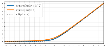
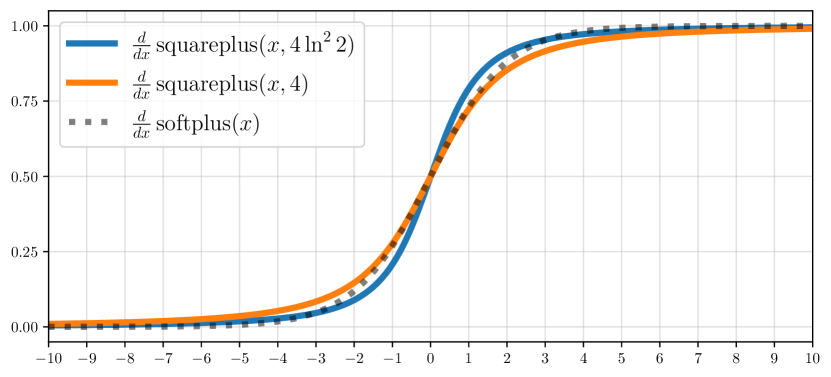
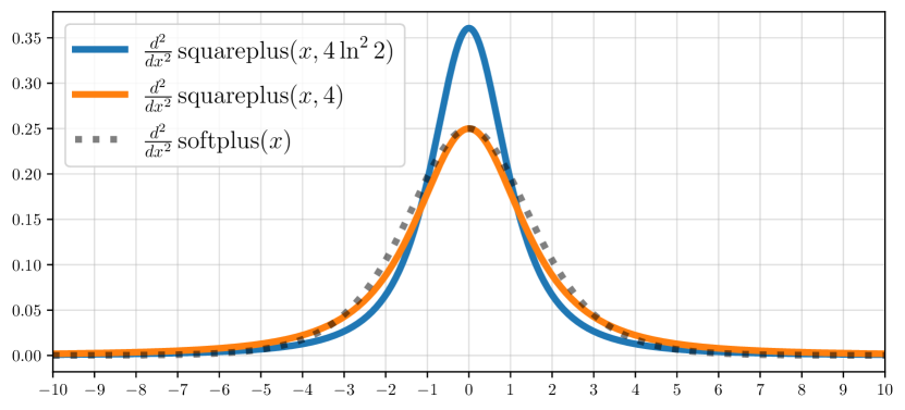
Figure 1: A visualization of softplus and two instances of squareplus with different values of the $b$ hyperparameter, as well as their first and second derivatives. Squareplus approximates softplus when $b=4\ln^{2}2$, and approximates its second derivative when $b=4$.

The first and second derivatives of squareplus are:

$$\frac{d}{dx}\,\operatorname{squareplus}(x,b) =\frac{1}{2}\left(1+\frac{x}{\sqrt{x^{2}+b}}\right)$$ (4)

$$\frac{d^{2}}{dx^{2}}\,\operatorname{squareplus}(x,b) =\frac{1}{2}\left(\frac{b}{(x^{2}+b)^{\nicefrac{{3}}{{2}}}}\right)$$ (5)

Like squareplus itself, these derivatives are algebraic and straightforward to compute efficiently. Analogously to how the derivative of a softplus is the classic logistic sigmoid function, the derivative of a squareplus is the “algebraic sigmoid” function $x/\sqrt{x^{2}+1}$ (scaled and shifted accordingly). And analogously to how the second derivative of a softplus is the PDF of a logistic distribution, the second derivative of a squareplus (with $b=2$) is the PDF of Student’s t-distribution (with $\nu=2$).

Specific values of the $b$ hyperparameter yield certain properties. When $b=0$, squareplus reduces to ReLU:

$$\operatorname{squareplus}(x,0)=\frac{x+|x|}{2}=\operatorname{relu}(x)$$ (6)

By setting $b=4\ln^{2}2$ we can approximate the shape of softplus near the origin:

$$\operatorname{squareplus}(0,4\ln^{2}2)=\operatorname{softplus}(0)$$ (7)

This is also the lowest value of $b$ where squareplus’s output is always guaranteed to be larger than softplus’s output:

$$\forall_{b\geq 4\ln^{2}2}\,\,\,\operatorname{squareplus}(x,b)\geq\operatorname{softplus}(x)$$ (8)

Setting $b=4$ causes squareplus’s second derivative to approximate softplus’s near the origin, and gives an output of $1$ at the origin (which the user may find intuitive):

$$\frac{d^{2}}{dx^{2}}\,\operatorname{squareplus}(0,4)=\frac{d^{2}}{dx^{2}}\operatorname{softplus}(0)=\frac{1}{4}$$ (9)

$$\operatorname{squareplus}(0,4)=1$$ (10)

For all valid values of $b$, the first derivative of squareplus is $\nicefrac{{1}}{{2}}$ at the origin, just as in softplus:

$$\forall_{b\geq 0}\,\,\ \frac{d}{dx}\operatorname{squareplus}(0,b)=\frac{d}{dx}\operatorname{softplus}(0)=\frac{1}{2}$$ (11)

The $b$ hyperparameter can be thought of as a scale parameter, analogously to how the offset in Charbonnier/pseudo-Huber loss can be parameterized as a scale parameter [1, 3]. As such, the same activation can be produced by scaling $x$ (and un-scaling the activation output) or by changing $b$:

$$\forall_{a>0}\,\,\,\frac{\operatorname{squareplus}(ax,b)}{a}=\operatorname{squareplus}\!\left(x,\frac{b}{a^{2}}\right)$$ (12)

Though squareplus superficially resembles softplus, when $|x|$ grows large squareplus approaches ReLU at a significantly slower rate than softplus. This is visualized in Figure 2, where we plot the difference between squareplus/softplus and ReLU. This figure also demonstrates the numerical instability of softplus on large inputs, which is why most softplus implementations return $x$ when $x\gg 0$. Similarly to this slow asymptotic behavior of the function itself, the gradient of squareplus approaches zero more slowly than that of softplus when $x\ll 0$. This property may be useful in practice, as ”dying” gradients are often undesirable, but presumably this is task-dependent.

	CPU	GPU
Softplus [5] (JAX impl.)	$3.777\text{\,}\mathrm{ms}$	$1.120\text{\,}\mathrm{ms}$
Softplus [5] (naive impl.)	$2.836\text{\,}\mathrm{ms}$	$1.118\text{\,}\mathrm{ms}$
ELU [4]	$2.040\text{\,}\mathrm{ms}$	$1.120\text{\,}\mathrm{ms}$
Swish/SiLU [6, 9, 11]	$1.234\text{\,}\mathrm{ms}$	$1.113\text{\,}\mathrm{ms}$
Relu [7, 8, 10]	$0.598\text{\,}\mathrm{ms}$	$1.069\text{\,}\mathrm{ms}$
Squareplus	$0.631\text{\,}\mathrm{ms}$	$1.074\text{\,}\mathrm{ms}$

Table 1: Runtimes on a CPU (for 1 million inputs) and a GPU (for 100 MM inputs) using JAX [2]. The “naive implementation” of softplus omits the special-casing necessary for softplus to produce finite values when $x$ is large.

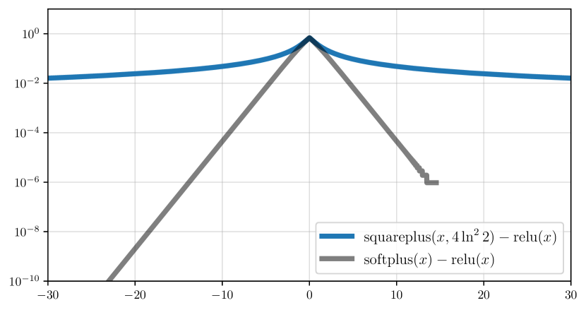
Figure 2: By visualizing the difference between squareplus/softplus and ReLU we see that squareplus approaches ReLU more slowly than softplus. The gray line terminates when softplus breaks down at $x\approx 15$, due to numerical instability.

As shown in Table 1, on a CPU squareplus is $\sim\!6\times$ faster than softplus, and is comparable to ReLU. On a GPU, squareplus is only $10\%$ faster than softplus, likely because all rectifiers are limited by memory bandwidth rather than computation in this setting. This suggests that squareplus may only be a desirable alternative to softplus in situations in which compute resources are limited, or when a softplus cannot be used — perhaps because $\exp$ and $\log$ are not supported by the hardware platform.

x

Acknowledgements: Thanks to the Twitter community for their helpful feedback to https://twitter.com/jon_barron/status/1387167648669048833

References

- [1] Jonathan T. Barron. A general and adaptive robust loss function. CVPR, 2019.
- [2] James Bradbury, Roy Frostig, Peter Hawkins, Matthew James Johnson, Chris Leary, Dougal Maclaurin, George Necula, Adam Paszke, Jake VanderPlas, Skye Wanderman-Milne, and Qiao Zhang. JAX: composable transformations of Python+NumPy programs, 2018.
- [3] P. Charbonnier, L. Blanc-Feraud, G. Aubert, and M. Barlaud. Two deterministic half-quadratic regularization algorithms for computed imaging. ICIP, 1994.
- [4] Djork-Arné Clevert, Thomas Unterthiner, and S. Hochreiter. Fast and accurate deep network learning by exponential linear units (ELUs). ICLR, 2016.
- [5] Charles Dugas, Yoshua Bengio, François Bélisle, Claude Nadeau, and René Garcia. Incorporating second-order functional knowledge for better option pricing. NIPS, 2000.
- [6] Stefan Elfwing, Eiji Uchibe, and Kenji Doya. Sigmoid-weighted linear units for neural network function approximation in reinforcement learning. Neural Networks, 2018. Special issue on deep reinforcement learning.
- [7] K. Fukushima. Visual feature extraction by a multilayered network of analog threshold elements. IEEE Trans. Syst. Sci. Cybern., 1969.
- [8] Xavier Glorot, Antoine Bordes, and Yoshua Bengio. Deep sparse rectifier neural networks. NIPS, 2011.
- [9] Dan Hendrycks and Kevin Gimpel. Bridging nonlinearities and stochastic regularizers with gaussian error linear units. CoRR, abs/1606.08415, 2016.
- [10] Jitendra Malik and Pietro Perona. Preattentive texture discrimination with early vision mechanisms. JOSA-A, 1990.
- [11] Prajit Ramachandran, Barret Zoph, and Quoc V. Le. Searching for activation functions. CoRR, abs/1710.05941, 2017.