Taking off the edge - simultaneous filament and end core formation

Abstract

Simulations of idealised star-forming filaments of finite length typically show core growth which is dominated by two cores forming at its respective end. The end cores form due to a strong increasing acceleration at the filament ends which leads to a sweep-up of material during the filament collapse along its axis. As this growth mode is typically faster than any other core formation mode in a filament, the end cores usually dominate in mass and density compared to other cores forming inside a filament. However, observations of star-forming filaments do not show this prevalence of cores at the filament ends. We explore a possible mechanism to slow the growth of the end cores using numerical simulations of simultaneous filament and embedded core formation, in our case a radially accreting filament forming in a finite converging flow. While such a setup still leads to end cores, they soon begin to move inwards and a density gradient is formed outside of the cores by the continued accumulation of material. As a result, the outermost cores are not longer located at the exact ends of the filament and the density gradient softens the inward gravitational acceleration of the cores. Therefore, the two end cores do not grow as fast as expected and thus do not dominate over other core formation modes in the filament.

1 Introduction

A vital step in the star-formation process is the fragmentation of gas from molecular clouds on scales of a few tens of parsecs down to individual star-forming cores with sizes of a few tenths of a parsec. Schneider & Elmegreen (1979) and Larson (1985) established the idea that this collapse does not happen directly but goes through an intermediate phase of filamentary fragmentation. Indeed, the dust observations of the Herschel space telescope (André et al., 2010) showed that molecular clouds are dominated by intricate networks of filaments which also are the locations where most cores are found (Arzoumanian et al., 2011; Könyves et al., 2015).

Many processes related to filament formation and their subsequent fragmentation are still unclear. Filamentary structure has been seen as a natural outcome of turbulent box simulations, with or without gravity (Vazquez-Semadeni, 1994; Klessen & Burkert, 2000; Padoan et al., 2001; Moeckel & Burkert, 2015; Federrath, 2016). These simulations have shown that they form by the compression of gas in the crossing of two planar shocks or as a consequence of dissipation at the end of the turbulent cascade (Kritsuk et al., 2013; Smith et al., 2014; Smith et al., 2016). The formation sites of stars are commonly situated in the densest regions where several filaments overlap with only few cores forming at the end of filamentary structure (Girichidis et al., 2014; Smith et al., 2014; Federrath, 2016). A similar morphology can be observed in collapsing cloud simulations (Dale & Bonnell, 2011; Bate, 2012; Gómez & Vázquez-Semadeni, 2014) where the global contraction usually leads to a central dense filament regulating the flow of gas from the cloud to the cores.

Nevertheless, simulations of individual, isolated filaments are dominated by a different morphology (Bastien, 1983; Bastien et al., 1991; Clarke & Whitworth, 2015; Seifried & Walch, 2015) with strong overdensities forming at both ends of the filament. This is due to the gravitational acceleration being the largest at the filament ends (Burkert & Hartmann, 2004; Pon et al., 2011, 2012; Toalá et al., 2012; Clarke & Whitworth, 2015), a concept which can be more generalised to more complex structures and which is known as so-called "gravitational focusing" or "edge-effect" (Burkert & Hartmann, 2004; Hartmann & Burkert, 2007; Li et al., 2016), where the magnitude of the gravitational acceleration scales with the curvature of the surface.

While there are observed cases of end dominated filaments (Zernickel et al., 2013; Kainulainen et al., 2016; Johnstone et al., 2017; Ohashi et al., 2018; Dewangan et al., 2019; Bhadari et al., 2020; Yuan et al., 2020; Cheng et al., 2021), the majority of observed filaments do not show a particular disposition to forming their most massive cores at their ends which can be due to several reasons. For instance, filaments forming in networks are interconnected and therefore do not have the density gradients at their ends required to form end cores. Nevertheless, one would expect the ends of the network to enhance core formation. Moreover, it has been shown that if filaments form with low aspect rations, large initial central overdensities or via filament mergers, the collapse of the gas is concentrated onto its centre (Keto & Burkert, 2014; Seifried & Walch, 2015; Hoemann et al., 2021), a morphology which has also been observed in large line-mass filaments (Kirk et al., 2013; Henshaw et al., 2014). Large central overdensities are however not expected in low-mass star forming filaments.

The discrepancy between theory and observations leads to the question whether different flow patterns in the formation of filaments can suppress dominant cores at the filament ends. In this paper we present such a process: the simultaneous migration of the forming end cores while the filament is under formation itself. In the turbulent formation regime, filaments form by colliding shocks leading to mass inflow on the cross-section of the shocks over a timescale which is given by the size of the inflow region and the shock velocity. While planar shocks first lead to the formation of sheets, these can further collapse and form filaments with sustained accretion along the plane of the sheet (Shimajiri et al., 2019; Chen et al., 2020). Moreover, direct gravitational collapse of cylindrically distributed material onto its centre will lead to a sustained radial inflow of gas (Clarke et al., 2017; Heigl et al., 2020) which can also be driven by the gravitational potential of the filament itself. While a purely gravitationally driven inflow makes the accretion of material outside of the end cores more unlikely, the process of simultaneous mass inflow and core migration can still occur. In our idealised simulations we assume a continuous radial inflow which replenishes the material outside of the end and stabilises the filamentary structure.

Accretion flows have been observed in many filaments (Schneider et al., 2010; Kirk et al., 2013; Palmeirim et al., 2013; Shimajiri et al., 2019; Bonne et al., 2020) and typically show estimated accretion rates of around $10-100$ M_⊙ pc^-1 Myr^-1 and accretion velocities of the order of $0.25-1.0$  km s^-1. If we assume a shock inflow region feeding the filament of around 0.5 pc, this would lead to a sustained inflow of material on timescales of 0.5-2 Myr. We demonstrate below that, while a filament is forming in such a sustained accretion flow, end cores will indeed begin to form and start migrating inwards while new material reforms the filament behind them. As we will show, this results in a suppression of the runaway growth of these cores and to core formation within the whole filament on roughly the same timescale.

The sections of the paper are organised as follows: section 2 discusses the basic physical principles which lead to the formation of cores at the filament ends. The numerical principles and initial conditions of the simulations are introduced in section 3 and their results are presented and discussed in section 4 and section 5. We draw the conclusions and summarise the results in section 6.

2 Basic concepts

While the edge-effect is not the only mode of core formation in filaments, it usually is the fastest. The end cores form at the position of the strong density gradient located at the ends of a filament due to the sharp increase in gravitational acceleration. Assuming a filament has a constant density $\rho$, a total length of $L$, a radius $R$ and that the filament is directed along the x-axis, this acceleration is given by (Burkert & Hartmann, 2004):

$$a_{x}=-2\uppi G\rho\left[2x-\sqrt{R^{2}+\left(L/2+x\right)^{2}}+\sqrt{R^{2}+\left(L/2-x\right)^{2}}\right]$$ (1)

with $G$ being the gravitational constant. The acceleration on the ends increases steeply for large aspect ratios which can be seen, for instance, in (Pon et al., 2012). For $x=L/2$ and large lengths $(L\gg R)$ this acceleration equals:

$$a_{x}=-2\uppi G\rho R.$$ (2)

In fact the acceleration increase is even stronger for more centralised radial profiles (Hoemann et al., 2022) such as the isothermal hydrostatic cylindrical profile (Stodólkiewicz, 1963; Ostriker, 1964):

$$\rho(r)=\frac{\rho_{\text{c}}}{\left(1+\left(r/H\right)^{2}\right)^{2}}$$ (3)

where $r$ is the cylindrical radius and $\rho_{\text{c}}$ is its central density. The radial scale height $H$ is given by the term:

$$H^{2}=\frac{2c_{\text{s}}^{2}}{\uppi G\rho_{\text{c}}}$$ (4)

where $c_{\text{s}}$ is the isothermal sound speed. This profile can only support a maximum mass per length in hydrostatic equilibrium. The maximum value is calculated by integrating the profile radially to infinity:

$$\left(\frac{M}{L}\right)_{\text{crit}}=\frac{2c_{\text{s}}^{2}}{G}$$ (5)

and one can define the parameter $f_{\text{cyl}}$ which gives the value of the current line-mass compared to the critical value (Fischera & Martin, 2012):

$$f_{\text{cyl}}=\left(\frac{M}{L}\right)/\left(\frac{M}{L}\right)_{\text{crit}}.$$ (6)

In pressure equilibrium with an ambient pressure, the hydrostatic radius of the isothermal filament is given by

$$R=H\left(\frac{f_{\text{cyl}}}{1-f_{\text{cyl}}}\right)^{1/2}=\left(\frac{2c_{\text{s}}^{4}}{\uppi Gp_{\text{ext}}}\left(f_{\text{cyl}}(1-f_{\text{cyl}})\right)\right)^{1/2}$$ (7)

as the central and outer density are connected by

$$\rho_{c}=\frac{\rho(R)}{(1-f_{\text{cyl}})^{2}}.$$ (8)

3 Numerical set-up

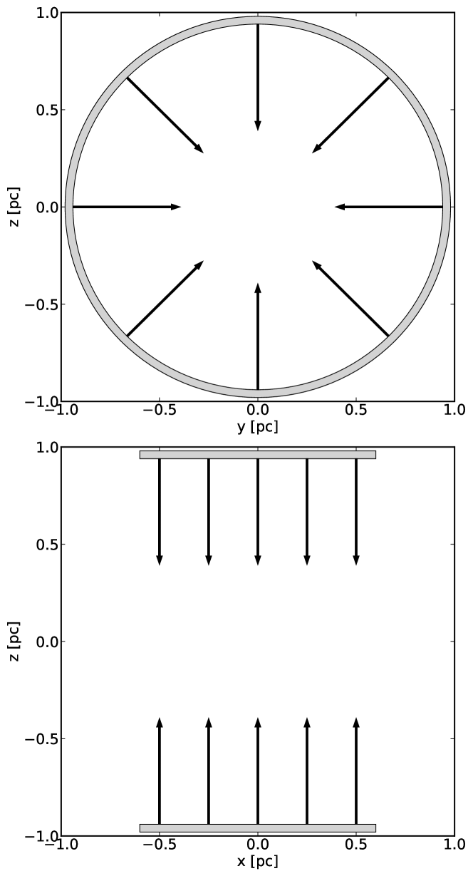
Figure 1: Schematic diagram of the inflow region as defined in the initial conditions. We show central cuts through the simulation box in the y-z and x-z plane. The inflow region where material is constantly replenished is given by the gray shaded region and the inflow velocity given to the gas is shown as arrows.

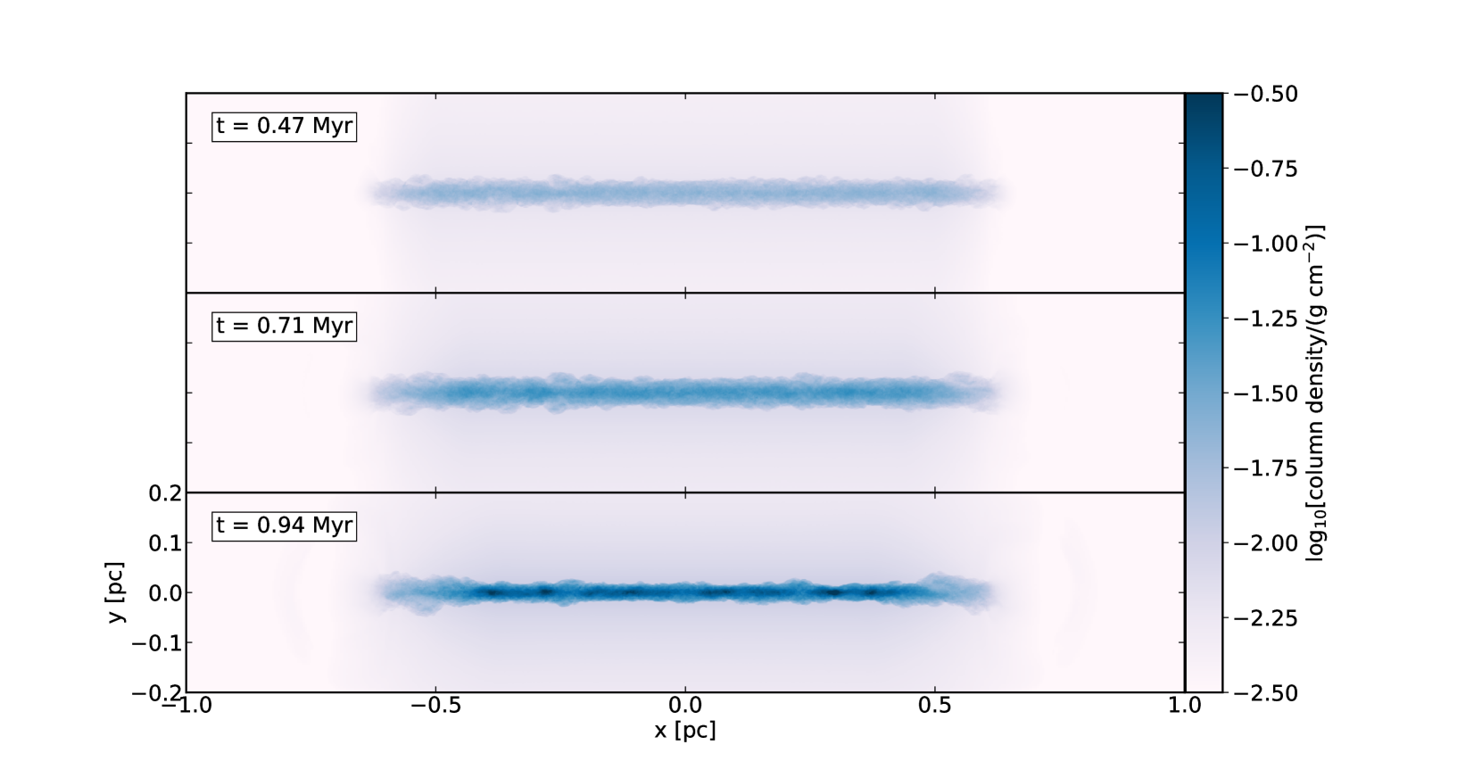
Figure 2: Overview of the simulation given by the density projection along the z-axis at different points in time. The radial accretion flow forms a turbulent filament which forms regularly spaced cores along its axis. The y-axis label is the same for every panel.

We ran our simulation with the code ramses (Teyssier, 2002) using a second-order Godunov scheme to solve the conservative form of the discretised Euler equations on an Cartesian grid. We applied the MUSCL scheme (Monotonic Upstream-Centred Scheme for Conservation Laws van Leer, 1979) in combination with the HLLC-Solver (Harten-Lax-van Leer-Contact Toro et al., 1994) and the multidimensional MC slope limiter (monotonized central-difference van Leer, 1977).

The formation and gravitational evolution of a finite-sized filament is simulated taking into account mass accretion from the surrounding. This is a key difference to previous simulations (Bastien, 1983; Bastien et al., 1991; Clarke & Whitworth, 2015; Seifried & Walch, 2015) that assumed an already existing filament and that followed its subsequent collapse. We do this by setting up a cylindrical inflow zone with a radius that is set in the y-z dimension and define a constant radial accretion flow onto the central x-axis, similar to the initial conditions of Heigl et al. (2018) and Heigl et al. (2020). In contrast to the former cases however, all boundaries of the box are set to open and we do not use a periodic boundary condition in x direction. In addition we limit the accretion flow to the central section of the box with a size of 0.6 times the box length. We choose the box to have a physical size of 2.0 pc resulting in an accretion zone with a radius of 1.0 pc and a length of 1.2 pc. A schematic diagram of inflow can be seen in Figure 1 where we show central cuts through the simulation box of the y-z and x-z plane.

The gas is set to be isothermal with a temperature of $10$ K with a molecular weight of $\mu=2.36$. In order to break the symmetry of the simulation, we introduce random density perturbations in the initial density and in the inflow following a flat distribution with a maximum value of 10% which allows the driving of turbulent motions. As shown in Heigl et al. (2018), the amplitude of the turbulence does not depend on the strength of the initial perturbation even when varied over close to four orders of magnitude ranging from 0.01% up to 50%. We do not set any preferred initial perturbation scale but vary every cell and let the cores form self-consistently from the resulting turbulence.

We set the mass accretion to a constant rate which is defined by the distance of the inflow zone to the central axis $R_{\text{0}}$, its density $\rho_{\text{0}}$ and the accretion velocity $v_{a}$:

$$\frac{\dot{M}}{L}=2\pi\rho_{0}R_{0}v_{a},$$ (9)

where both of the latter values are renewed at every timestep in the simulation. The constant mass accretion set at the radius $R_{\text{0}}$ propagates inward and leads to a radial density profile outside of the forming filament of:

$$\rho(r)=\frac{\rho_{\text{0}}R_{\text{0}}}{r}.$$ (10)

We vary the value of the accretion rate in different simulations by adjusting the density $\rho_{\text{0}}$ and the accretion velocity $v_{a}$.

As the filament diameter itself is only a fraction of the total box size and as we are not interested in the details of the accretion flow itself, we employ adaptive mesh refinement (AMR) in order to speed up the simulation by increasing the resolution inside the filament and keeping the resolution low in the ambient medium. We vary the resolution level from 8 to 12 which means that our base grid has a resolution of $256^{3}$, corresponding to a cell size of $7.8\times 10^{-3}$ pc, whereas our filament is resolved by a resolution of $4096^{3}$, corresponding to a cell size of $4.9\times 10^{-4}$ pc. As a refinement condition we use the Truelove criterion (Truelove et al., 1997) increasing the resolution as soon as the Jeans length is not resolved by 256 cells. We choose an aggressive refinement value of 256 in order to guarantee that the filament is resolved fully with our highest resolution. We stop the simulation as soon as a core collapses and we do not fulfill the Truelove criterion for our highest refinement level anymore.

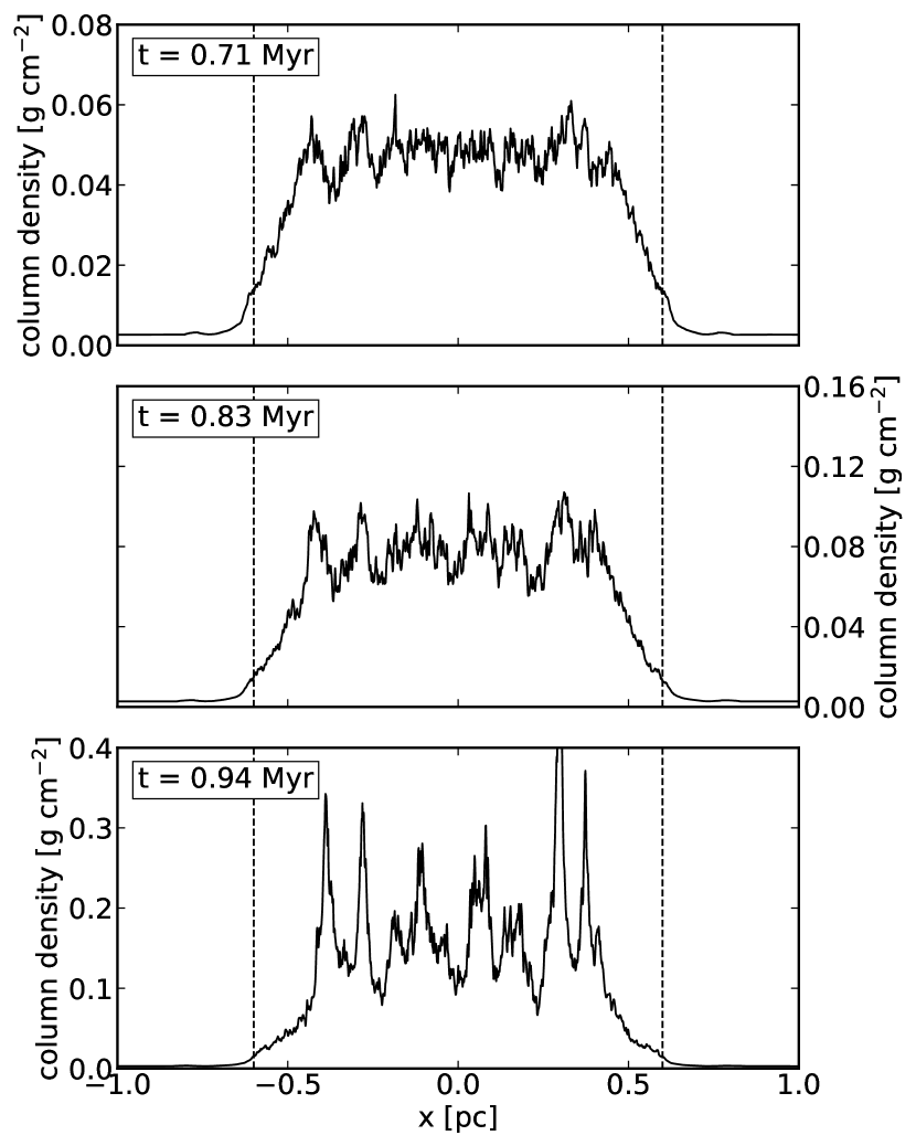
Figure 3: Time evolution of the column density in z direction along the central x-axis. The inflow region is marked by the vertical dashed lines. In contrast to developing dominant end cores, the inner dense region stays relatively even. The filament contracts over time and forms equally dense cores along its axis. The x-axis label applies to every panel.

4 General results

As a fiducial case study we set the initial density in the box and that of the accretion flow to a mean value of $3.92\times 10^{-22}$  g cm^-3, corresponding to a number density of about $100$  cm^-3. The inflow velocity is set to a value of $0.75$  km s^-1, which is equal to a Mach number of 4.0 for 10 K gas. The resulting accretion rate is therefore about $27.9$ M_⊙ pc^-1 Myr^-1 which is consistent with predicted and observed accretion rates and velocities (Schneider et al., 2010; Kirk et al., 2013; Palmeirim et al., 2013; Shimajiri et al., 2019; Bonne et al., 2020). However, as we do not include an initial accretion profile of the form of Equation 10 in this case, the accretion rate will be lower in the beginning and will grow to the constant value as soon as the accretion profile is established.

Here we provide a detailed analysis of our general findings starting with an overview of the evolution of the filament in Figure 2. We plot the column density along the z-axis assuming our gas is optically thin. The different panels show different time steps of the simulation. As the material streams to the box centre it forms a filament which gains mass over time. In addition, the inflow stabilises the filament against radial expansion. One can clearly see the turbulent nature of the gas which is driven by the dissipative accretion shock and a smooth density gradient at the two end points of the filament ends extending into the ambient medium. A tentative imprint of the inflow region can be seen in column density as slightly darker region around the filament itself. Other than its straight form due to the nature of how we defined the filament accretion, the visual impression closely resembles observed filamentary structure.

While a pre-defined, non-accreting filament would immediately start forming end cores, most of the evolution of the accreting filament is uneventful. As it grows in mass over time it becomes denser while retaining a relatively soft gradient in column density to the ambient medium. After about 0.7 Myr, cores condense out of the filament material with none being particularly dominant compared to the others. The last snapshot of the simulation is shown in the third panel where one can see several cores along the filament with similar spacing. Note that the outermost cores do not coincide with the filament ends.

In addition to the slices, we also show column density cuts along the central axis in Figure 3 where the evolution of the overdensities can be seen in more detail. The first panel shows the earliest stage of overdensities forming in the filament at 0.71 Myrs. Although material is accreted in the region between $x=-0.6$ and $x=0.6$, one can already see that the densest part is shorter and forms a central dense region which contracts over time. We will concentrate on this region, which we will address as dense inner region, in further dynamical investigations as it contains most of the filament material. While for a non-accreting filament a contraction along the filament axis would lead to an enhancement of material in the filament ends, in this case the accreting filament shows a homogeneous increase along its axis with only small density fluctuations. The next panel at 0.83 Myrs shows a time step where several cores have formed. While there are also two overdensities forming at the end of the inner dense region, these do not form earlier than the rest and have similar column densities as the other cores. While the inner dense region contracts along the filament axis, one can see that the continuous inflow brings in new material around its ends. The last panel at at 0.94 Myrs shows the last time step of the simulation where one of the cores begins to collapse leading to a drastic increase in its central column density. Interestingly, it is not one of the outermost ones as one would expect for an end dominated filament but the second from the right. Again, neglecting the collapsing one, all cores have similar central column densities albeit with a possible tendency of the outer cores to be slightly denser.

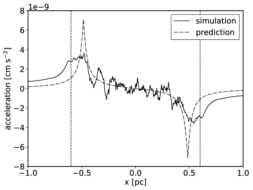
Figure 4: Gravitational acceleration along the filament axis for t=0.83 Myr. The solid curve shows the measured acceleration in the simulation while the dashed-dotted curve is the analytic prediction of Equation 10 for the dense inner region. The inflow region is marked by the dashed vertical lines. There is a considerable softening of the acceleration at the positions of the end cores.

The reason for the difference in the importance of the end cores compared to the collapse of an non-accreting filament has to lie in the acceleration at the filament ends. We therefore analyse the output at 0.83 Myrs in more detail. First, we plot the measured gravitational acceleration along the filament in the simulation as the solid curve in Figure 4 together with the analytical prediction of Equation 10 where we use the length, the mean density and the mean radius of the dense inner region. We define the length of the dense inner region by the distance between the outer edges of the outermost cores which we find by determining the two points where the column density first exceeds the mean column density of the dense inner region calculated in a section between -0.25 pc and 0.25 pc. As the column density is relatively flat, taking the mean of an inner section smoothes out possible over- and underdensities. Within the dense inner region the prediction agrees very well with the measured acceleration. However, at its ends, where the end cores form, it differs strongly. The material outside of the outermost cores leads to a softening of the gravitational attraction at the position of the end cores. As the ends of the inner region are more and more embedded in newly accreted material, the acceleration at their position matches more a region contained inside a filament. As the new density gradient is very shallow, the new ends are evenly accelerated instead of leading to a sweep-up of material.

In general, this result should be independent of the density profile of the filament as a soft filament end should always decrease the acceleration at the end of a filament. However, as we are also interested in the question whether we can apply analytical perturbation theory which has been established for the hydrostatic profile of Equation 3, we furthermore plot the density profile perpendicular to the filament radially averaged over the dense inner region in Figure 5. In the plot one can discern two distinct regions which are composed of the filament itself and the accretion region. The accretion region follows an $r^{-1}$ profile as established in Equation 10 until it hits the filament surface where an accretion shock is formed and a jump in density occurs. The filament itself follows well the hydrostatic solution which is defined by the central density and given in the plot by the dashed black line. It does so despite the filament containing turbulent motions as was already the case in Heigl et al. (2020) as the turbulence only adds a constant background pressure. We will use this fact for analysing core distances in the next section.

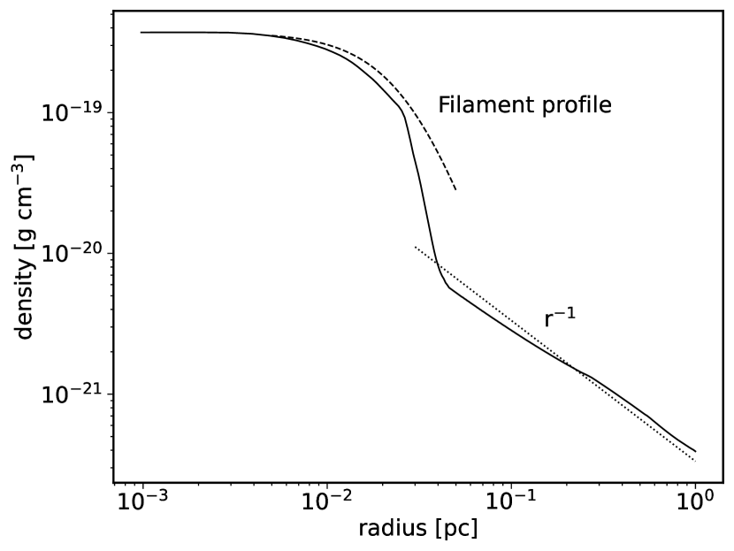
Figure 5: Radial density profile of the filament and the surrounding accretion region at 0.83 Myrs. We average the density along the filament axis inside the dense inner region. The filament follows the hydrostatic solution of Equation 3 which is defined by its central density and shown by the dashed line. The accretion region follows an $r^{-1}$ profile in agreement for a constant accretion rate set by the boundary values in the accretion zone as given in Equation 10.

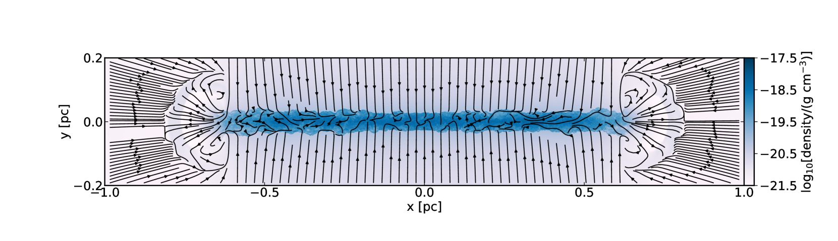
Figure 6: Density slice through the centre of the filament at 0.83 Myr. The streamlines show the direction of the velocity in the plain of the slice. One can see that material at the filament ends is flowing into the ambient medium where it forms shock fronts.

An interesting consequence of the radial compression of the gas is that a small amount of material is pushed out at the filament ends due to the pressure gradient from the dense compressed material to the ambient medium. This leads to a small shocked region surrounding both filament ends. Although this feature is very hard to detect in the column density of Figure 2, it can be seen in the density slice through the centre of the filament shown in Figure 6. In addition to the density, we also show the direction of the velocity vectors in the plane of the slice overlaid as streamlines. One can see the inflow region accreting onto the filament, the ambient medium being gravitationally pulled towards the filament and the two outflow regions pushing against it. While the density of the outflow regions is very thin, shock fronts form where they hit and compress the ambient medium. Wether such outflow features can be detected in observations is an interesting question, its thin density however makes such observations challenging. Note that the outflows do not affect the overall evolution of the filament itself as the mass loss rate of about $\sim 0.1$ M_⊙ Myr^-1 at both ends is negligible small compared to the total mass accretion rate of $27.9$ M_⊙ Myr^-1.

5 Core separation

A key question of filamentary fragmentation theory and of star formation is the existence of a quasi-regular core spacing. This mode of fragmentation has been predicted by hydrostatic models, as there exists a dominant mode for which the growth time scale of the overdensities is the shortest (Stodólkiewicz, 1963; Larson, 1985; Nagasawa, 1987; Inutsuka & Miyama, 1992; Nakamura et al., 1993; Gehman et al., 1996). Observations of core spacing have been inconclusive with several studies showing lower separations than expected (André et al., 2010; Kainulainen et al., 2013; Teixeira et al., 2016) with some agreeing with the predictions (Beuther et al., 2015; Contreras et al., 2016; Kainulainen et al., 2016). Consequently, the core separation in our simulations is of considerable interest.

The predicted dominant mode of fragmentation in filaments is calculated from the polynomial approximation

$$y(f_{\text{cyl}})=\sum_{i=0}^{5}a_{i}f_{\text{cyl}}^{i/2}$$ (11)

with the respective values $a_{i}$ shown in table E.1 of Fischera & Martin (2012) which are also listed in Table 1. Here, y represents either the length scale $\lambda_{dom}$, the dominant fragmentation length in units of 1/FWHM, with FWHM being the full width half maximum of the filament profile, or the length scale FWHM itself in units of 1/$H$. This means we can express the dominant fragmentation length as function of the current average line-mass $f_{\text{cyl}}$ and the current average scale height $H$ and therefore by extension the current average central density. This leads to a major complication for verifying the theoretical predictions, not only in simulations, but also in observations. In an accreting filament the average line-mass constantly increases and the average central density changes over time. However, one can only measure the current average line-mass and the current average central density at a single point in time and not the line-mass and central density that the filament had when the cores began forming. While in principle one could follow the core growth in simulations from the beginning, it is impossible to measure the core separation at their time of birth directly as the cores are indiscernible from other turbulent perturbations at this point of time. Moreover, a further complication is that the length of the filament and consequently the distance between cores will decrease over time due to the gravitational collapse along its axis. At a single point in time, one can only measure the current spacing.

However, if the cores in the simulation all began to form at the same time and thus all formed at the same dominant fragmentation length, we can test if we can determine this point in time. While the cores in principle can form independently at any time there are two key observations which lead to the assumption that all cores are seeded on the same dominant wavelength:

• the cores seem all to appear at the same time and evolve on similar timescales

• we generally do not see any cores sub-fragmenting and merging

This means that the number of cores which are present at the end of the simulation are a consequence of the imprint of the singular dominant wavelength when the cores began to grow. Even as their distance between each other lessens over time due to the collapse of the dense inner region, we can backtrace their mean separation, determined by the number of cores and the length of the dense inner region, in order to see if it matches the prediction of the co-evolving dominant fragmentation length.

Table 1: Constants of the polynomial approximation of the predicted dominant fragmentation length for the values calculated in Nagasawa (1987) as listed in Fischera & Martin (2012). FWHM is the full width half maximum of the filament profile and $\tau_{\text{dom}}$ is the growth time of the dominant mode in units of $\sqrt{4\pi G\rho_{c}}$.

	$a_{0}$	$a_{1}$	$a_{2}$	$a_{3}$	$a_{4}$	$a_{5}$
$\lambda_{\text{dom}}/\text{FWHM}$	6.25	0.00	-6.89	9.18	-3.44	0.00
$\text{FWHM}/H$	0.00	1.732	0.00	-0.041	0.818	-0.976
$\tau_{\text{dom}}\sqrt{4\pi G\rho_{c}}$	4.08	0.00	-2.99	1.46	0.40	0.00

With the purpose of conducting a statistical study on the number of cores which form in accreting filaments, we perform a new set of simulations. In contrast to the fiducial case, we now introduce several changes in order to keep the mass accretion rate as close to constant as possible which enables us to map the line-mass to a certain time in the simulation more easily. Therefore, the velocity and density of the material reaching the filament have to be kept constant. For low accretion Mach numbers, the gravitational acceleration acting upon the gas starting at the edge of the box with a size 2.0 pc can already increase the accretion velocity significantly once the gas reaches the filament. We prevent this by using a larger accretion Mach number of 6.0 for which we do not see any significant increase in velocity. Furthermore, as the density and the mass accretion rate of the ambient medium is only constant if the density profile follows Equation 10, we also include it as the initial density profile at the start of the simulation. In order to obtain a better statistical sample of the number of cores and compare different accretion rates, we perform two sets of simulations which we repeat ten times each with varying initial seeds for the perturbations and use the mean of the number of cores. The accretion rate is varied by setting the accretion density in the inflow region to $n_{\text{0}}=25.0$  cm^-3, corresponding to $\rho_{\text{0}}=9.80\times 10^{-23}$  g cm^-3, and $n_{\text{0}}=50.0$  cm^-3, corresponding to $\rho_{\text{0}}=1.96\times 10^{-22}$  g cm^-3with respective accretion rates of 10.5 and 21.0 $\text{M}_{\odot}\text{ pc}^{-1}\text{ Myr}^{-1}$. For larger accretion rates the number of cores which form are too numerous to be reliably distinguished from each other. Therefore, we do not include larger accretion rates in our simulations.

The expected dominant fragmentation length is determined for all simulations at every output time by calculating the mean central density and mean line-mass of the dense inner region and using these values in Equation 11. We show the resulting evolution of the fragmentation length in Figure 7 as the bundle of semi-transparent solid lines. One can see that the dominant fragmentation length rises over time unit it reaches a plateau after which it starts to fall again until we stop the simulations due to the collapse of a core. The form of the curves follows the evolution of the scale height which evolves similar for increasing line-mass and has its maximum at $f_{\text{cyl}}=0.5$. The curves all show similar values with some differences due to the initial random seed which grow over time. For larger accretion rates, the dominant fragmentation length is shorter and fragmentation happens faster which is consistent with analytical models due to the larger central density and the smaller scale height.

We compare the dominant fragmentation length predicted by theory to the mean core separation we measure in our simulations. The mean core separation is calculated by dividing the length of the dense inner region, the region which is undergoing fragmentation, by the number of cores counted at the end of the simulation minus one in order to take into account the end cores. We determine the length of the inner dense region as described before by locating the outer end of the end cores where the column density rises above the mean column density inside the dense inner region. Since the inner dense region is not defined at the start of the simulation, we use the length of the total inflow region of 1.2 pc as theoretical value of the inner region. Note, that this definition also gives us an artificial core separation value even before the cores began to form. This however is intended as we do not know the point in time when the cores form and as we are interested if we can determine it by matching the backtraced core separation to the dominant fragmentation length.

In order to count the number of cores, we determine the number of overdensities in the last output file as seen in Figure 3. Doing this towards the end of the simulation has the additional advantage of more evolved cores which makes them easier to distinguish from small fluctuations in the filament. As the cores have varying central densities, column densities and line-masses, there is no general good criteria for classifying a particular overdensity as a core. Therefore, we use the output of the clump finder algorithm employed by ramses to determine the number of cores. The algorithm uses a ’watershed’ segmentation in order to find connected dense regions above a given density threshold. It uses an automatic noise reduction and allows for merging of peaks above a given ratio of central to saddle density called ’relevance’. More details can be found in Bleuler et al. (2015). As we only want to detect the overdensities in the central region, we set the density threshold to a typical central density of a filament of $n=10^{5}$  cm^-3. In addition, in order to reduce noise, we set the relevance threshold to 3.0 and only use clumps which have reached a minimum mass of 0.1 solar masses. Using this method we determine the mean core number over all ten different realisations for increasing accretion rate to be 3.0 and 8.3 with a standard deviation of 0.77 and 1.19, respectively. There is some variation with the number of cores depending on how large we set the relevance and the mass threshold with the mass threshold showing a larger influence. Adapting a much smaller mass threshold of 0.01 solar masses however only increases the number of cores by a factor of around 10%.

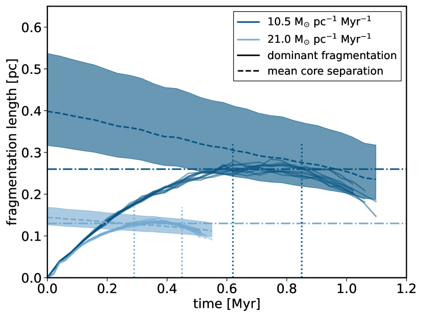
Figure 7: Evolution of the dominant fragmentation length and the core separation over time for different accretion rates. The bundle of solid lines shows the values of the dominant fragmentation length as calculated from the simulations starting with different initial seeds. The dashed lines show the mean core separation determined by measuring the mean length of the dense inner region over time and dividing it by the mean number of cores. The corresponding error bars, given by the filled shaded area, show the standard deviation which follows from the variation of the number of cores in the different simulations. Both distributions show an overlap close to the peak of the dominant fragmentation lengths given by the horizontal dashed-dotted lines. We indicate the length of the time period where the dominant fragmentation length is close to the peak value by the vertical dotted lines.

We plot the mean core separation over time in Figure 7 as the dashed line together with its standard deviation resulting from the variability in core numbers as the shaded area. As the inner dense region collapses along its axis the mean core separation decreases over time. Compared to the theoretically expected dominant fragmentation length, one can see that for early times the distributions do not match, but as soon as the peak of the dominant fragmentation is reached there is a direct overlap with the mean core separation after which the dominant fragmentation shows a trend of falling below the core separation again. This overlap could indicate that cores are generally seeded when the dominant fragmentation reaches its peak. However, this is only a first order approach as the dominant fragmentation length is constantly changing. Nevertheless, one can see from the broadness of the peak of the dominant fragmentation length that the filaments spend a considerable amount of time at similar dominant fragmentation lengths indicated by the horizontal dashed-dotted lines. For smaller and larger times the change in dominant fragmentation length is much faster so any change in line-mass would affect the dominant fragmentation length much more. Therefore, perturbations seeded at the peak of the dominant fragmentation length could potentially grow close to the seed mode longer than at any other point in the filament’s evolution. This could lead to an initial core growth which is strong enough to exceed other modes at earlier and later times even if the dominant fragmentation length is constantly changing.

In order to verify the compatibility of our theory we measure the time spent by the filament at the peak of the curve as given by the vertical dotted lines which is from 0.62 Myrs to 0.85 Myrs for the low accretion rate and from 0.29 to 0.45 Myrs for the large accretion rate, respectively. For both accretion rates we determine the mean e-folding growth time The e-folding timescales of the dominant fragmentation length are given by the corresponding values in table E.1 of Fischera & Martin (2012) for the polynomial approximation

$$\tau_{\text{dom}}(f_{\text{cyl}})\cdot\sqrt{4\pi G\rho_{c}}=\sum_{i=0}^{5}a_{i}f_{\text{cyl}}^{i/3}$$ (12)

and are listed in Table 1. As it depends on the line-mass of the filament, we map the respective points in time to the line-mass as can be seen in Figure 8 where we plot the evolution of the line-mass over time. We show the measured mean line-mass for each simulation as a bundle of semi-transparent solid lines together with the expectation if the inner dense region would not collapse as the dashes lines. In this case the line-mass would increase linearly over time, however, as the inner dense region is shortening it increases faster than in the non-collapsing case as more material is concentrated in a shorter structure. The vertical dotted lines mark the same points in time as in Figure 7. The interpolated mean line-masses at the beginning and the end of the time period close to the peak are similar in both cases, 0.43 to 0.61 for the low accretion case and 0.40 to 0.63 for the large accretion case, and are shown as filled shaded areas. Using the marked points in time as bounding cases, we insert the growing mean line-mass and corresponding mean central density in Equation 12 and calculate the respective mean e-folding timescale over this time period for each simulation separately. Finally, we take the mean of these values for the respective accretion rate. For both the low and large accretion rate the timescales match well. The time spent close to the peak value is given by 0.23 and 0.16 Myrs respectively, while the mean dominant e-folding time is 0.17 and 0.11 Myrs. This demonstrates that cores seeded at the peak of the curve of the dominant fragmentation length have enough time to grow for more than an e-folding time and therefore could exceed earlier and later modes as these have less time to grow at their respective dominant fragmentation length. Thus, we see a tentative indication that the analytic predictions of the hydrostatic model are consistent with the fragmentation in simulated accreting filaments.

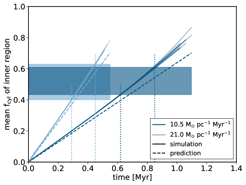
Figure 8: Evolution of the mean line-mass in units of $f_{\text{cyl}}$ of the dense inner region over time for different mass accretion rates. The measured mean line-mass of all simulations is given by the solid lines and the predicted mean line-mass from a constant mass accretion rate as given by the legend is shown by the dashed lines. The vertical dotted lines indicate the time period in where the dominant fragmentation length is close to the peak value as given by Figure 7 and the filled shaded areas show the respective interpolated values of the mean line-mass.

In general, increasing the accretion rate leads to the formation of more cores. This is to be expected as a larger accretion rate leads to a larger ram pressure onto the filament which increases its central density which in turn lowers the dominant fragmentation length. However, from the core separation alone one cannot derive the accretion rate as the same ram pressure can be achieved by varying numbers of accretion density and velocity. Nevertheless, one can use the observed core separation as an indicator of the ambient pressure. As one can see in Figure 7, at least for larger accretion rates, the line-mass of the filament grows faster than the central dense region contracts which results in a flattening of the measured core separation for larger values of the filament line-mass. If one now assumes that the cores are seeded at values of $f_{\text{cyl}}\approx 0.4-0.6$, one can in principle estimate the ambient pressure of the surrounding medium leading to a corresponding dominant fragmentation length.

6 Discussion and conclusions

While our simulations show that a continuous accretion does prevent the formation of dominant end cores, several additional questions remain.

An intriguing puzzle is the tendency of observations to find narrower core separations in large line-mass filaments than what is predicted by theory (André et al., 2010; Kainulainen et al., 2013; Teixeira et al., 2016). Our analysis of expected fragmentation lengths presented in Figure 7 shows that for large times the dominant fragmentation decreases faster than the inner region contracts. Therefore, in contrast to observations, the predicted fragmentation length is usually shorter than what we measure in simulations. This could be an indication that such a hydrostatic model is not applicable for all filaments.

However, the shapes of the curves formed by the dominant fragmentation length shown in Figure 7 are very likely to change depending on the mass accretion onto the filament and turbulence within. We presented a very idealised model with a constant mass accretion rate without initial turbulent motions. A more realistic case with varying mass accretion rate and turbulent motions in the accreted material is very likely to shift the peak of the curves. Thus, the values of $f_{\text{cyl}}\approx 0.4-0.6$ at which the cores are likely seeded in our simulations should not be applied necessarily to all accreting filaments. Nevertheless, if the dominant fragmentation length shows a peak, due to the timescale argument presented in section 5 it is likely that cores will form with a preferred separation close to the peak value.

A surprising side effect of the model is the creation of outflows at the filament ends. This effect however could be reduced by non-homogeneous inflows with low density at the shock front ends. Due to their low density and mass loading, these outflow would be very hard to detect and as far as we know there is no observation of such an phenomena to date. A possible tracer of the outflow would be the shock heating or chemical shock traces in the ambient medium as the material streams out with large velocities.

Finally, it will be interesting to explore whether our results remain valid in the case of planar accretion flows instead of radial geometries. Depending on the extent, a planar shock will not create a filamentary morphology but lead to a sheet between the shock fronts. However, as soon as enough material has been concentrated and gravity takes over, this sheet could collapse and be collected into a filamentary structure. We will explore if this mode of filament formation shows the same effect on end core formation as presented here in a future study.

To summarise, we have presented a numerical study on the simultaneous filament and end core formation. We have shown that while end cores do form at the ends of the central dense region, they do not dominate over the cores formed by regular perturbation growth. This is due to the material which is replenished continuously from the inflow outside of the contracting inner region which leads to a reduced gravitational acceleration at its ends and a soft edge morphology. Comparing the measured core separation in our idealised simulations to the dominant fragmentation length shows a tentative agreement that cores are seeded at $f_{\text{cyl}}\approx 0.4-0.6$. The comparison is not straight-forward due to a continuously shifting dominant fragmentation length over time, however an accreting filament spends a considerable amount of time in this line-mass region where the dominant fragmentation length only changes slightly. This means that cores seeded at these values have about an e-folding timescale to grow and therefore exceed later core formation modes. Independent of the core separation, we presented a valid mechanism to form a filament morphology which is not dominated by the edge effect as was the goal of the paper.

Data Availability

The data underlying this article will be shared on reasonable request to the corresponding author.

References

- André et al. (2010) André P., et al., 2010, A&A, 518, L102
- Arzoumanian et al. (2011) Arzoumanian D., et al., 2011, A&A, 529, L6
- Bastien (1983) Bastien P., 1983, A&A, 119, 109
- Bastien et al. (1991) Bastien P., Arcoragi J.-P., Benz W., Bonnell I., Martel H., 1991, ApJ, 378, 255
- Bate (2012) Bate M. R., 2012, MNRAS, 419, 3115
- Beuther et al. (2015) Beuther H., Ragan S. E., Johnston K., Henning T., Hacar A., Kainulainen J. T., 2015, A&A, 584, A67
- Bhadari et al. (2020) Bhadari N. K., Dewangan L. K., Pirogov L. E., Ojha D. K., 2020, ApJ, 899, 167
- Bleuler et al. (2015) Bleuler A., Teyssier R., Carassou S., Martizzi D., 2015, Computational Astrophysics and Cosmology, 2, 5
- Bonne et al. (2020) Bonne L., et al., 2020, A&A, 641, A17
- Burkert & Hartmann (2004) Burkert A., Hartmann L., 2004, ApJ, 616, 288
- Chen et al. (2020) Chen C.-Y., Mundy L. G., Ostriker E. C., Storm S., Dhabal A., 2020, MNRAS, 494, 3675
- Cheng et al. (2021) Cheng Y., et al., 2021, ApJ, 916, 78
- Clarke & Whitworth (2015) Clarke S. D., Whitworth A. P., 2015, MNRAS, 449, 1819
- Clarke et al. (2017) Clarke S. D., Whitworth A. P., Duarte-Cabral A., Hubber D. A., 2017, MNRAS, 468, 2489
- Contreras et al. (2016) Contreras Y., Garay G., Rathborne J. M., Sanhueza P., 2016, MNRAS, 456, 2041
- Dale & Bonnell (2011) Dale J. E., Bonnell I., 2011, MNRAS, 414, 321
- Dewangan et al. (2019) Dewangan L. K., Pirogov L. E., Ryabukhina O. L., Ojha D. K., Zinchenko I., 2019, ApJ, 877, 1
- Federrath (2016) Federrath C., 2016, MNRAS, 457, 375
- Fischera & Martin (2012) Fischera J., Martin P. G., 2012, A&A, 542, A77
- Gehman et al. (1996) Gehman C. S., Adams F. C., Fatuzzo M., Watkins R., 1996, ApJ, 457, 718
- Girichidis et al. (2014) Girichidis P., Konstandin L., Whitworth A. P., Klessen R. S., 2014, ApJ, 781, 91
- Gómez & Vázquez-Semadeni (2014) Gómez G. C., Vázquez-Semadeni E., 2014, ApJ, 791, 124
- Hartmann & Burkert (2007) Hartmann L., Burkert A., 2007, ApJ, 654, 988
- Heigl et al. (2018) Heigl S., Burkert A., Gritschneder M., 2018, MNRAS, 474, 4881
- Heigl et al. (2020) Heigl S., Gritschneder M., Burkert A., 2020, MNRAS, 495, 758
- Henshaw et al. (2014) Henshaw J. D., Caselli P., Fontani F., Jiménez-Serra I., Tan J. C., 2014, MNRAS, 440, 2860
- Hoemann et al. (2021) Hoemann E., Heigl S., Burkert A., 2021, MNRAS, 507, 3486
- Hoemann et al. (2022) Hoemann E., Heigl S., Burkert A., 2022, arXiv e-prints, p. arXiv:2203.07002
- Inutsuka & Miyama (1992) Inutsuka S.-I., Miyama S. M., 1992, ApJ, 388, 392
- Johnstone et al. (2017) Johnstone D., et al., 2017, ApJ, 836, 132
- Kainulainen et al. (2013) Kainulainen J., Ragan S. E., Henning T., Stutz A., 2013, A&A, 557, A120
- Kainulainen et al. (2016) Kainulainen J., Hacar A., Alves J., Beuther H., Bouy H., Tafalla M., 2016, A&A, 586, A27
- Keto & Burkert (2014) Keto E., Burkert A., 2014, MNRAS, 441, 1468
- Kirk et al. (2013) Kirk H., Myers P. C., Bourke T. L., Gutermuth R. A., Hedden A., Wilson G. W., 2013, ApJ, 766, 115
- Klessen & Burkert (2000) Klessen R. S., Burkert A., 2000, ApJS, 128, 287
- Könyves et al. (2015) Könyves V., et al., 2015, A&A, 584, A91
- Kritsuk et al. (2013) Kritsuk A. G., Lee C. T., Norman M. L., 2013, MNRAS, 436, 3247
- Larson (1985) Larson R. B., 1985, MNRAS, 214, 379
- Li et al. (2016) Li G.-X., Burkert A., Megeath T., Wyrowski F., 2016, arXiv e-prints, p. arXiv:1603.05720
- Moeckel & Burkert (2015) Moeckel N., Burkert A., 2015, ApJ, 807, 67
- Nagasawa (1987) Nagasawa M., 1987, Progress of Theoretical Physics, 77, 635
- Nakamura et al. (1993) Nakamura F., Hanawa T., Nakano T., 1993, PASJ, 45, 551
- Ohashi et al. (2018) Ohashi S., Sanhueza P., Sakai N., Kandori R., Choi M., Hirota T., Nguyen-Lu’o’ng Q., Tatematsu K., 2018, ApJ, 856, 147
- Ostriker (1964) Ostriker J., 1964, ApJ, 140, 1056
- Padoan et al. (2001) Padoan P., Juvela M., Goodman A. A., Nordlund Å., 2001, ApJ, 553, 227
- Palmeirim et al. (2013) Palmeirim P., et al., 2013, A&A, 550, A38
- Pon et al. (2011) Pon A., Johnstone D., Heitsch F., 2011, ApJ, 740, 88
- Pon et al. (2012) Pon A., Toalá J. A., Johnstone D., Vázquez-Semadeni E., Heitsch F., Gómez G. C., 2012, ApJ, 756, 145
- Schneider & Elmegreen (1979) Schneider S., Elmegreen B. G., 1979, ApJS, 41, 87
- Schneider et al. (2010) Schneider N., Csengeri T., Bontemps S., Motte F., Simon R., Hennebelle P., Federrath C., Klessen R., 2010, A&A, 520, A49
- Seifried & Walch (2015) Seifried D., Walch S., 2015, MNRAS, 452, 2410
- Shimajiri et al. (2019) Shimajiri Y., André P., Palmeirim P., Arzoumanian D., Bracco A., Könyves V., Ntormousi E., Ladjelate B., 2019, A&A, 623, A16
- Smith et al. (2014) Smith R. J., Glover S. C. O., Klessen R. S., 2014, MNRAS, 445, 2900
- Smith et al. (2016) Smith R. J., Glover S. C. O., Klessen R. S., Fuller G. A., 2016, MNRAS, 455, 3640
- Stodólkiewicz (1963) Stodólkiewicz J. S., 1963, Acta Astron., 13, 30
- Teixeira et al. (2016) Teixeira P. S., Takahashi S., Zapata L. A., Ho P. T. P., 2016, A&A, 587, A47
- Teyssier (2002) Teyssier R., 2002, A&A, 385, 337
- Toalá et al. (2012) Toalá J. A., Vázquez-Semadeni E., Gómez G. C., 2012, ApJ, 744, 190
- Toro et al. (1994) Toro E., Spruce M., Speares W., 1994, Shock Waves, 4, 25
- Truelove et al. (1997) Truelove J. K., Klein R. I., McKee C. F., Holliman II J. H., Howell L. H., Greenough J. A., 1997, ApJ, 489, L179
- Vazquez-Semadeni (1994) Vazquez-Semadeni E., 1994, ApJ, 423, 681
- Yuan et al. (2020) Yuan L., et al., 2020, A&A, 637, A67
- Zernickel et al. (2013) Zernickel A., Schilke P., Smith R. J., 2013, A&A, 554, L2
- van Leer (1977) van Leer B., 1977, Journal of Computational Physics, 23, 276
- van Leer (1979) van Leer B., 1979, Journal of Computational Physics, 32, 101