Data-driven design of safe control for polynomial systems

Abstract

We consider the problem of designing an invariant set using only a finite set of input-state data collected from an unknown polynomial system in continuous time. We consider noisy data, i.e., corrupted by an unknown-but-bounded disturbance. We derive a data-dependent sum-of-squares program that enforces invariance of a set and also optimizes the size of the invariant set while keeping it within a set of user-defined safety constraints; the solution of this program directly provides a polynomial invariant set and a state-feedback controller. We numerically test the design on a system of two platooning cars.

, , ,

1 Introduction

Control systems are nowadays required not only to stabilize the process around a desired working point given by an equilibrium, but also to be able to steer away the state of the system from dangerous regions where it would not work properly. The complement of this dangerous set is the so-called safe set and the design of control schemes to respect safety specifications goes by the name of safe control [17, 38, 35, 33]. The notion of safety is intuitively related to the notion of invariance, namely, the dynamical propriety that the state belongs to a certain set for all subsequent times after being initialized in there. Historically, a seminal result for invariance was Nagumo’s theorem [29], which has been of fundamental importance in the characterization of invariant sets for continuous-time systems. Since almost every system in practice is subject to some type of constraints on its states or outputs, the notion of invariance is very relevant in control applications to include safety constraints in the design. Indeed, problems related to safety and viability [4] can be addressed by computing sets possessing invariance or closely-related properties.

In the control community, invariance for linear systems was extensively studied in the 1980-1990’s, which resulted in a number of works surveyed in [8]. For nonlinear systems, there has recently been a revived interest with the introduction of control Lyapunov-like functions tailored to enforce invariance, called control barrier functions [40, 39, 36, 32]. In this setting, the controller depends critically on the model used for design and recent studies [20, 16, 25] focus on finding robust safe controllers to account for possibly inaccurate models. In [3], unmodeled dynamics are taken into account by adding a bounded disturbance on the input to find a robust control barrier function, in an input-to-state-safety fashion.

In an effort to reduce this critical dependence from the model, we implement a data-driven solution for safe control. This work follows on from [6] on enforcing invariance with a controller designed directly from data and it extends [6] to the case of polynomial nonlinear systems and by dropping the assumption that the set to make invariant is given. Polynomial systems are a notable class of nonlinear systems widely used to model processes in engineering applications such as fluid dynamics [10, 22] and robotics [26]. Casting nonlinear control design as an optimization problem faces the obstacle that it is generally computationally intractable to verify whether a multivariate (matrix) polynomial is nonnegative. For a computationally viable approach, one can adopt a relaxation and verify instead whether such a polynomial is a sum-of-squares (SOS) since SOS optimization can be solved through semidefinite programming (SDP) [31, 11]. In a model-based setting, SOS programs have been used to design stabilizing controllers for hybrid systems [30], for disturbance analysis in linear systems [21] and to obtain inner-approximations of the basin of attraction [34], to name a few applications.

Still, SOS programs suffer from some limitations that have been or are being addressed in the literature. A first one is scalability of SOS programs: tools are available [24] that automatically reduce the problem size without major computational costs, and recent works on large-scale semidefinite and polynomial optimization [41] improve scalability of SOS programs significantly. Secondly, it is often the case that the obtained SOS program is bilinear in the decision variables. This occurs in the model-based case [34] and also in this paper. An iterative approach to solve these bilinear SOS programs is commonly used [21]. Alternatively, there exist tools to solve these bilinear SOS programs directly, such as PENBMI and BMIBNB. For these reasons, the limitations of SOS programs seem largely outweighed by their positive features.

From the side of (direct) data-driven control, this work is positioned in the literature thread [27, 12, 15], to name a few, which exploits the so-called fundamental lemma in [37, Th. 1]. Within this thread, [6, 14, 18, 5] are the most closely related works to this one. As mentioned before, [6] addresses also an invariance problem, but for systems with linear dynamics and where the set to be rendered invariant is given. The works [14, 18] and [5, §5] consider nonlinear input-affine polynomial systems as here, but the goal is data-driven almost global [14] or global [18, 5] stabilization; invariance is a fairly weaker dynamical property (e.g., solutions do not need to converge to an attractor within the invariant set), hence the conditions here are fairly less conservative and yet significant to enforce safety.

Contribution. Our contribution is to enforce invariance using no model of the system to be controlled, but only a set of input-state data points collected from it in an experiment. We consider an input-affine nonlinear system with polynomial dynamics and a polynomial controller. This allows us to make the data-based invariance conditions tractable by using an SOS relaxation and alternately solving two SOS programs. In this work we consider the realistic setting when invariance needs to be guaranteed despite the presence of an unknown-but-bounded [19] additive noise in data. Moreover, we show that also in the data-driven case it is possible to optimize the size of the invariant set while respecting safety constraints. Finally, we provide numerical evidence to show the effectiveness of the approach, in particular on the practical example of two platooning cars.

Structure. Section 2 recalls the theory enabling our results. In Section 3, we set up the invariance problem for polynomial systems. In Section 4, we derive a data-driven controller that solves the invariance problem, and also includes safety constraints. In Section 5, we exemplify our data-based solution for two platooning cars.

Notation. For a matrix $A$, $A^{\top}$ denotes its transpose. A symmetric matrix $A\in\mathbb{R}^{n\times n}$ is positive semidefinite, i.e., $A\succeq 0$, if $x^{\top}Ax\geq 0$ for all $x\in\mathbb{R}^{n}$. Given two matrices $A$ and $B$, $A\succeq B$ means $A-B\succeq 0$. With $\mathbb{Z}_{\geq 0}$ we indicate the set of nonnegative integers. An identity matrix is denoted by $I$. For a positive semidefinite $A=A^{\top}$, $A^{1/2}$ denotes the unique positive semidefinite root of $A$. For matrices $M$ and $N=N^{\top}$, we sometimes abbreviate $MNM^{\top}$ as $MNM^{\top}=M\cdot N[\star]^{\top}$. For symmetric matrices $A$ and $C$, we sometimes abbreviate the symmetric matrix $\left[\begin{smallmatrix}A&B^{\top}\\ B&C\end{smallmatrix}\right]$ as $\left[\begin{smallmatrix}A&\star\\ B&C\end{smallmatrix}\right]$ or $\left[\begin{smallmatrix}A&B^{\top}\\ \star&C\end{smallmatrix}\right]$.

2 Preliminaries

In this section, we present a fundamental result from real algebraic geometry, the Positivstellensatz. We first report from [11, 21] the notions needed to state that result.

We start from sum-of-squares (SOS) polynomials and SOS matrix polynomials. A function $h:\mathbb{R}^{n}\rightarrow\mathbb{R}$ is a monomial of degree $d$ in $x=(x_{1},x_{2},\dots,x_{n})\in\mathbb{R}^{n}$ if

$$h(x)=ax_{1}^{q_{1}}x_{2}^{q_{2}}\cdots x_{n}^{q_{n}}$$

with $a\in\mathbb{R}$, $q_{1},\dots,q_{n}\in\mathbb{Z}_{\geq 0}$ and $d=\sum_{i=1}^{n}q_{i}$. A function $h:\mathbb{R}^{n}\rightarrow\mathbb{R}$ is a polynomial if it is a sum of (a finite number of) monomials $h_{1}$, $h_{2},\ldots:\mathbb{R}^{n}\rightarrow\mathbb{R}$ with finite degree, and the largest degree of the $h_{i}$’s is the degree of $h$. $\Pi$ denotes the set of polynomials.

Definition 1 (SOS polynomial).

$h\in\Pi$ is an SOS polynomial if there exist $h_{1},\dots,h_{k}\in\Pi$ such that $h(x)=\sum_{i=1}^{k}h_{i}(x)^{2}$. The set of SOS polynomials $h\in\Pi$ is denoted as $\Sigma$.

A function $H:\mathbb{R}^{n}\to\mathbb{R}^{r_{1}\times r_{2}}$ is a matrix polynomial if the entries of $H$ satisfy $h_{ij}\in\Pi$ for all $i=1$, …, $r_{1}$ and $j=1$, …, $r_{2}$, and the largest degree of the entries of $H$ is the degree of $H$. The set of matrix polynomials $H:\mathbb{R}^{n}\to\mathbb{R}^{r_{1}\times r_{2}}$ is denoted by $\Pi_{r_{1},r_{2}}$. A function $H:\mathbb{R}^{n}\to\mathbb{R}^{r_{1}\times r_{2}}$ is a square matrix polynomial if $r_{1}=r_{2}$. The set of square matrix polynomials $H:\mathbb{R}^{n}\to\mathbb{R}^{r\times r}$ is denoted by $\Pi_{r}$.

Definition 2 (SOS matrix polynomial [11]).

$H\in\Pi_{r}$ is an SOS matrix polynomial if there exist $H_{1}$, …, $H_{k}\in\Pi_{r}$ such that $H(x)=\sum_{i=1}^{k}H_{i}(x)^{\top}H_{i}(x)$. The set of SOS matrix polynomials $H\in\Pi_{r}$ is denoted by $\Sigma_{r}$.

SOS polynomials are instrumental to define three sets of polynomials appearing in the Positivstellensatz.

Definition 3 (Multiplicative monoid [21, Def. 3]).

Given $g_{1}$, …, $g_{t}\in\Pi$, the multiplicative monoid generated by $g_{j}$’s is the set of all finite products of $g_{j}$’s, including $1$ (i.e., the empty product). It is denoted by $\mathcal{M}(g_{1},\dots,g_{t})$, with $\mathcal{M}(\emptyset):=1$ for completeness.

An example is $\mathcal{M}(g_{1},g_{2})=\{g_{1}^{k_{1}}g_{2}^{k_{2}}\colon k_{1},k_{2}\in\mathbb{Z}_{\geq 0}\}$.

Definition 4 (Cone [21, Def. 4]).

Given $f_{1},\dots,f_{r}\in\Pi$, the cone generated by $f_{i}$’s is $\mathcal{C}(f_{1},\ldots,f_{r}):=\big{\{}s_{0}+\sum_{i=1}^{l}s_{i}b_{i}\colon l\in\mathbb{Z}_{\geq 0},s_{i}\in\Sigma,b_{i}\in\mathcal{M}(f_{1},\ldots,f_{r})\big{\}}$.

If $s\in\Sigma$ and $f\in\Pi$, then $f^{2}s\in\Sigma$. Then, a cone of $\{f_{1},\dots,f_{r}\}$ can be expressed as a sum of $2^{r}$ terms without loss of generality. An example is $\mathcal{C}(f_{1},f_{2})=$ $\{s_{0}+s_{1}f_{1}+s_{2}f_{2}+s_{3}f_{1}f_{2}\colon s_{0},\dots,s_{3}\in\Sigma\}$ where terms like $s_{4}f_{1}^{2}$ or $s_{5}f_{2}^{2}$ with $s_{4}$, $s_{5}\in\Sigma$ are not needed since they are captured by $s_{0}$ anyway.

Definition 5 (Ideal [21, Def. 5]).

Given $h_{1},\dots,h_{u}\in\Pi$, the ideal generated by $h_{k}$’s is $\mathcal{J}(h_{1},\dots,h_{u}):=\{\sum_{k=1}^{u}h_{k}p_{k}\colon p_{k}\in\Pi\}$.

An example is $\mathcal{J}(h_{1},h_{2})=\{h_{1}p_{1}+h_{2}p_{2}\colon p_{1},p_{2}\in\Pi\}$. With Definitions 3-5, we finally recall the version in [21] of the Positivstellensatz (P-Satz), in the next fact.

Fact 1 (P-Satz [21, Th. 1]).

Given $f_{1},\dots,f_{r}\in\Pi$, $g_{1},\dots,g_{t}\in\Pi$, and $h_{1},\dots,h_{u}\in\Pi$, the following are equivalent.

1. The set

   $$\left\{x\in\mathbb{R}^{n}\colon\begin{array}[]{c}f_{1}(x)\geq 0,\dots,f_{r}(x)\geq 0\\ g_{1}(x)\neq 0,\dots,g_{t}(x)\neq 0\\ h_{1}(x)=0,\dots,h_{u}(x)=0\end{array}\right\}=\emptyset.$$

2. There exist polynomials $f\in\mathcal{C}(f_{1},\dots,f_{r})$, $g\in\mathcal{M}(g_{1},\dots,g_{t})$, $h\in\mathcal{J}(h_{1},\dots,h_{u})$ such that

   $$f+g^{2}+h=0.$$

3 Collecting data and enforcing invariance

In this paper we consider polynomial systems of the form

$$\dot{x}=f(x)+g(x)u$$ (1)

where $x\in\mathbb{R}^{n}$ is the state, $u\in\mathbb{R}^{m}$ is the control input, $f$ and $g$ are polynomial vector fields. The specific expressions of $f$ and $g$ are unknown. The polynomial system (1) can be written into the linear-like form

$$\dot{x}=\mathsf{A}Z(x)+\mathsf{B}W(x)u$$ (2)

where $\mathsf{A}\in\mathbb{R}^{n\times N_{\mathsf{A}}}$ and $\mathsf{B}\in\mathbb{R}^{n\times N_{\mathsf{B}}}$ are unknown constant matrices, the known $N_{\mathsf{A}}\times 1$ vector $Z(x)$ contains as entries the distinct monomials in $x$ that may appear in $f$, and the known $N_{\mathsf{B}}\times m$ matrix $W(x)$ contains as entries the monomials that may appear in $g$. The conditions we will propose to design an invariant set are the same regardless of the choice of the monomials in $Z$ and $W$. On the other hand, different choices of $Z$ and $W$ affect feasibility and goodness of the solution arising from those conditions, as is generally the case with model structure selection. In Section 5, we will present guidelines for the choice of monomials in $Z$ and $W$.

We consider the control law $u=K(x)$ where $K\in\Pi_{m,1}$ is to be designed. The closed-loop dynamics results in

$$\!\dot{x} =\mathsf{A}Z(x)+\mathsf{B}W(x)K(x)=\begin{bmatrix}\mathsf{A}&\mathsf{B}\end{bmatrix}\begin{bmatrix}Z(x)\\ W(x)K(x)\end{bmatrix}.$$ (3)

Data are generated through an experiment in the presence of an additive disturbance $d$ as

$$\dot{x}=\mathsf{A}Z(x)+\mathsf{B}W(x)u+d.$$ (4)

We apply an input sequence of $T$ elements, and measure the state and state derivative sequences generated by (4); we sample uniformly these sequences at times $0$, $\tau_{\textup{s}}$, …, $(T-1)\tau_{\textup{s}}$ for sampling period $\tau_{\textup{s}}>0$; this results in data points, for $j=0,\dots,T-1$,

$$\dot{x}^{j}:=\dot{x}(j\tau_{\textup{s}}),\,z^{j}:=Z(x(j\tau_{\textup{s}})),\,v^{j}:=W(x(j\tau_{\textup{s}}))u(j\tau_{\textup{s}}).$$ (5)

A disturbance sequence given for $j=0,\dots,T-1$ by

$$d^{j}:=d(j\tau_{\textup{s}})$$

acts during the experiment but is unknown. Hence, the data generation mechanism is described by

$$\dot{x}^{j}=\mathsf{A}z^{j}+\mathsf{B}v^{j}+d^{j},j=0,1,\dots,T-1.$$ (6)

Our goal is to use the collected data points to obtain an invariant set for (3) as specified in the next definition.

Definition 3.1 (Invariant set).

For $a\colon\mathbb{R}^{n}\to\mathbb{R}^{n}$ polynomial, i.e., $a\in\Pi_{n,1}$, and for an arbitrary $x_{0}\in\mathbb{R}^{n}$, denote $t\mapsto\alpha(t,x_{0})$ the (unique maximal) solution to $\dot{x}=a(x)$ with initial condition $x_{0}=\alpha(0,x_{0})$ and defined on the interval $[0,T(x_{0}))$ (with $T(x_{0})$ possibly $+\infty$). A set $\mathcal{I}$ is said to be invariant for $\dot{x}=a(x)$ if $x_{0}\in\mathcal{I}$ implies that for all $t\in[0,T(x_{0}))$, $\alpha(t,x_{0})\in\mathcal{I}$.

Consider the set

$$\mathcal{I}:=\{x\in\mathbb{R}^{n}:h(x)\leq 0\}$$ (7)

with $h\in\Pi$. To impose that $\mathcal{I}$ is an invariant set according to Definition 3.1, we require the condition

$$\{x\in\mathbb{R}^{n}:h(x)=0\}\subseteq\{x\in\mathbb{R}^{n}:\frac{\partial h}{\partial x}(x)\dot{x}\leq-\epsilon\}$$ (8)

where $\dot{x}$, used for brevity, takes the expression in (3) and the parameter $\epsilon>0$ is introduced to guarantee some degree of robustness at the boundary of $\mathcal{I}$.

Remark 3.2.

We emphasize that whereas we use noisy data for control design as per the data generation mechanism in (6), we design a controller to enforce nominal invariance for $d=0$ as in (3), instead of robust invariance. Nonetheless, our design features some degree of robustness thanks to $\epsilon$, as we now show. Define the nominal closed-loop vector field in (3) as $f_{\textup{n}}(x):=\mathsf{A}Z(x)+\mathsf{B}W(x)K(x)$ and consider now the perturbed dynamics $\dot{x}=f_{\textup{n}}(x)+d$ with $|d|^{2}\leq\omega$ (as we will have later in (12)). $\mathcal{I}$ is robustly invariant for this perturbed dynamics as long as

$$\tfrac{\partial h}{\partial x}(x)(f_{\textup{n}}(x)+d)\leq 0\quad\forall(x,d)\colon h(x)=0,|d|^{2}\leq\omega$$ (9)

By achieving (8), we have that for all $x$ and $d$ with $h(x)=0$ and $|d|^{2}\leq\omega$,

$$\tfrac{\partial h}{\partial x}(x)(f_{\textup{n}}(x)+d)\leq-\epsilon+\left|\tfrac{\partial h}{\partial x}(x)\right|\sqrt{\omega}.$$

Then, robust invariance in (9) is achieved if $\left|\tfrac{\partial h}{\partial x}(x)\right|\leq\epsilon/\sqrt{\omega}$ for all $x$ such that $h(x)=0$ or, equivalently, if

$$\begin{bmatrix}-\epsilon^{2}/\omega&\tfrac{\partial h}{\partial x}(x)\\ \tfrac{\partial h}{\partial x}(x)^{\top}&-I\end{bmatrix}\preceq 0\quad\forall x\colon h(x)=0,$$

which can be relaxed into an SOS condition and added to our optimization program (see later Theorem 4.10). For these reasons, we rather consider for simplicity nominal invariance and introduce $\epsilon>0$ to guarantee nonetheless some degree of robustness at the boundary of $\mathcal{I}$.

With the goal of applying Fact 1, (8) can be cast as

$$\begin{split}\Big{\{}x\in\mathbb{R}^{n}:\ &h(x)=0,\\ &\frac{\partial h}{\partial x}(x)\dot{x}+\epsilon\geq 0,\ \frac{\partial h}{\partial x}(x)\dot{x}+\epsilon\neq 0\Big{\}}=\emptyset.\end{split}$$

This empty set condition is equivalent, by Fact 1, to the existence of $\ell_{1}\in\Pi$, $s_{0},s_{1}\in\Sigma$ and $k_{1}\in\mathbb{Z}_{\geq 0}$ such that

$$\ell_{1}h+s_{0}+s_{1}\Big{(}\frac{\partial h}{\partial x}\dot{x}+\epsilon\Big{)}+\Big{(}\frac{\partial h}{\partial x}\dot{x}+\epsilon\Big{)}^{2k_{1}}=0.$$ (10)

With the final goal of implementing numerically this condition, we simplify (10) by setting $s_{0}=0$, $k_{1}=1$ and $\ell_{1}=\ell\big{(}\frac{\partial h}{\partial x}\dot{x}+\epsilon\big{)}$ and, for $\ell\in\Pi$ and $s_{1}\in\Sigma$, obtain

$$\Big{(}\frac{\partial h}{\partial x}\dot{x}+\epsilon\Big{)}\Big{[}\ell h+s_{1}+\Big{(}\frac{\partial h}{\partial x}\dot{x}+\epsilon\Big{)}\Big{]}=0,$$

which is a relaxation of (10). So, the original (8) is implied by

$$\ell(x)h(x)+\frac{\partial h}{\partial x}(x)\dot{x}+\epsilon=-s_{1}(x)\leq 0\qquad\forall x.$$ (11)

The arguments above can be summarized as follows.

Lemma 3.3.

If there exists $\ell\in\Pi$ such that condition (11) holds, then $\mathcal{I}$ in (7) is an invariant set for (4).

Indeed, for all $x$ such that $h(x)=0$ (corresponding to the boundary of $\mathcal{I}$), the condition imposes $\frac{\partial h}{\partial x}(x)\dot{x}\leq-\epsilon$, i.e., the Lie derivative of $h$ is strictly negative. For all $x$ such that $h(x)<0$ (corresponding to the interior of $\mathcal{I}$), the condition imposes $\frac{\partial h}{\partial x}(x)\dot{x}\leq-\epsilon-\ell(x)h(x)$. Since $\ell$ is a polynomial without any sign definiteness requirement and $\epsilon$ is a design parameter selected as a small positive number, the term $-\epsilon-\ell(x)h(x)$ does not need to be negative and can actually be positive; hence, the condition may allow even for a positive $\frac{\partial h}{\partial x}(x)\dot{x}$, consistently with set invariance being less restrictive than attractivity.

4 Data-driven safe control

Our goal is to formulate a condition depending exclusively on noisy data to find an invariant set for the actual system (3). We substitute in (11) the closed-loop dynamics in (3) and obtain

$$\ell(x)h(x)+\epsilon+\frac{\partial h}{\partial x}(x)\begin{bmatrix}\mathsf{A}&\mathsf{B}\end{bmatrix}\begin{bmatrix}Z(x)\\ W(x)K(x)\end{bmatrix}\leq 0\quad\forall x.$$

Since the model is not available and the true coefficient matrices $\mathsf{A}$ and $\mathsf{B}$ are unknown, we rather enforce the previous inequality on all matrices $(A,B)$ that are consistent with data (for a given disturbance model), as we now characterize. By consistent with data, we mean all matrices $(A,B)$ that could have produced the measured data sequences $\{\dot{x}^{j},z^{j},v^{j}\}_{j=0}^{T-1}$ as in (5) for an additive disturbance $d$ that is bounded. A realistic bound on disturbance is that the norm of any possible disturbance instance $d$ is upper-bounded, and so are the norms of the unknown $d^{0}$, …, $d^{T-1}$. This corresponds to an instantaneous bound given, for $\omega\geq 0$, by the set

$$\mathcal{D}_{\textup{i}}:=\{d\in\mathbb{R}^{n}:|d|^{2}\leq\omega\}.$$ (12)

Then, based on the bound in $\mathcal{D}_{\textup{i}}$, the matrices $(A,B)$ consistent with a single data point $j\in\{0,\dots,T-1\}$ belong to the set

$$\mathcal{C}^{j}_{\textup{i}}:= \Big{\{}[A\ B]\colon\dot{x}^{j}=Az^{j}+Bv^{j}+d,\,dd^{\top}\preceq\omega I\Big{\}},$$ (13)

$$= \Big{\{}[A\ B]\colon\begin{bmatrix}I&A&B\end{bmatrix}\begin{bmatrix}I&\dot{x}^{j}\\ 0&-z^{j}\\ 0&-v^{j}\end{bmatrix}\cdoT\begin{bmatrix}\omega I&0\\ 0&-I\end{bmatrix}[\star]^{\top}\!\succeq 0\Big{\}}.$$

$\mathcal{C}^{j}_{\textup{i}}$ is the set of all matrices for which some disturbance $d$ satisfying the bound in (12) could have generated the measured data point $j$, as in [28, 13]. The set of matrices $(A,B)$ consistent with all data points $j=0,\dots,T-1$ is then

$$\mathcal{C}_{\textup{i}}:=\bigcap_{j=0}^{T-1}\mathcal{C}^{j}_{\textup{i}}.$$ (14)

We discussed in [7] that, for matrices $\zeta_{0}$, $P=P^{\top}\succ 0$, $Q=Q^{\top}\succeq 0$, the set $\mathcal{C}_{\textup{i}}$ cannot be expressed as a matrix ellipsoid of the form

$$\{\zeta\in\mathbb{R}^{(n+m)\times n}\colon(\zeta-\zeta_{0})^{\top}P^{-2}(\zeta-\zeta_{0})\preceq Q\},$$ (15)

which is instrumental to obtain our main result. On the other hand, this form can be obtained for the matrix ellipsoid $\overline{\mathcal{C}}_{\textup{i}}$ defined for $A_{\textup{i}}\succ 0$ as

$$\overline{\mathcal{C}}_{\textup{i}}:=\{[A\ B]=\zeta^{\top}\colon$$

$$\hskip 28.45274pt\begin{bmatrix}I&\zeta^{\top}\end{bmatrix}\begin{bmatrix}B_{\textup{i}}^{\top}A_{\textup{i}}^{-1}B_{\textup{i}}-I~{}&B_{\textup{i}}^{\top}\\ B_{\textup{i}}~{}&A_{\textup{i}}\end{bmatrix}\begin{bmatrix}I\\ \zeta\end{bmatrix}\preceq 0\}.$$ (16)

Indeed, for $A_{\textup{i}}\succ 0$, the condition in (16) is precisely $(\zeta+A_{\textup{i}}^{-1}B_{\textup{i}})^{\top}A_{\textup{i}}(\zeta+A_{\textup{i}}^{-1}B_{\textup{i}})\preceq I$, so that the selections

$$\overline{\zeta}_{\textup{i}}:=-A_{\textup{i}}^{-1}B_{\textup{i}},\quad\overline{P}_{\textup{i}}^{-2}:=A_{\textup{i}},\quad\overline{Q}_{\textup{i}}:=I$$ (17)

rewrite $\overline{\mathcal{C}}_{\textup{i}}$ equivalently as

$$\overline{\mathcal{C}}_{\textup{i}} =\{[A\ B]=\zeta^{\top}:(\zeta-\overline{\zeta}_{\textup{i}})^{\top}\overline{P}_{\textup{i}}^{-2}(\zeta-\overline{\zeta}_{\textup{i}})\preceq\overline{Q}_{\textup{i}}\}.$$ (18)

In summary, because the form (18) allows us to obtain our main result, we over-approximate $\mathcal{C}_{\textup{i}}$ in (14) through $\overline{\mathcal{C}}_{\textup{i}}$ in (16) where the matrices $A_{\textup{i}}\succ 0$ and $B_{\textup{i}}$ are determined by solving an optimization program, which we recall from [7, § 5.1].

From data, define for $j=0,\dots,T-1$

$$c_{j}:=-\omega I+\dot{x}^{j}(\dot{x}^{j})^{\top},$$

$$b_{j}:=-\begin{bmatrix}z^{j}\\ v^{j}\end{bmatrix}(\dot{x}^{j})^{\top},a_{j}:=\begin{bmatrix}z^{j}\\ v^{j}\end{bmatrix}\begin{bmatrix}z^{j}\\ v^{j}\end{bmatrix}^{\top}.$$ (19)

As it is done for classical ellipsoids [9, §3.7.2], we impose that the matrix ellipsoid $\overline{\mathcal{C}}_{\textup{i}}$, which is well-defined for $A_{\textup{i}}\succ 0$, includes $\mathcal{C}_{\textup{i}}$ through the (lossy) S-procedure [9, §2.6.3] and we then minimize the size of $\overline{\mathcal{C}}_{\textup{i}}$. This corresponds to the optimization program

$$\begin{split}&\text{minimize}\ -\log\det A_{\textup{i}}\\ &\text{subject to}\\ &\ \begin{bmatrix}\vspace*{1pt}-I-\sum_{j=0}^{T-1}\tau_{j}c_{j}&B_{\textup{i}}^{\top}-\sum_{j=0}^{T-1}\tau_{j}b_{j}^{\top}&B_{\textup{i}}^{\top}\\ \vspace*{1pt}B_{\textup{i}}-\sum_{j=0}^{T-1}\tau_{j}b_{j}&A_{\textup{i}}-\sum_{j=0}^{T-1}\tau_{j}a_{j}&0\\ B_{\textup{i}}&0&-A_{\textup{i}}\end{bmatrix}\preceq 0,\\ &\ A_{\textup{i}}\succ 0,\ \tau_{j}\geq 0\text{ for }j=0,\dots,T-1.\end{split}$$ (20)

When this optimization program is solved, we use the returned $A_{\textup{i}}$ and $B_{\textup{i}}$ to obtain the matrices $\overline{\zeta}_{\textup{i}}$, $\overline{P}_{\textup{i}}$ $\overline{Q}_{\textup{i}}$ as in (17). Before further analyzing the optimization program, we discuss in the next remark an alternative bound on the disturbance that is commonly used.

Remark 4.4.

When an instantaneous bound on the disturbance is given by $|d|^{2}\leq\omega$ as in $\mathcal{D}_{\textup{i}}$ in (12), one can infer that the whole unknown disturbance sequence $\begin{bmatrix}d^{0}&\dots&d^{T-1}\end{bmatrix}$ of the experiment belongs to the set

$$\mathcal{D}_{\textup{e}}:=\{D\in\mathbb{R}^{n\times T}:DD^{\top}\preceq T\omega I\},$$ (21)

which we call an energy bound on the disturbance. By collecting data points in (5) in matrices

$$X_{1} :=\begin{bmatrix}\dot{x}^{0}&\dots&\dot{x}^{T-1}\end{bmatrix},$$ (22a)

$$Z_{0} :=\begin{bmatrix}z^{0}&\dots&z^{T-1}\end{bmatrix},V_{0}:=\begin{bmatrix}v^{0}&\dots&v^{T-1}\end{bmatrix},$$ (22b)

the set of matrices consistent with data is

$$\begin{split}\!&\mathcal{C}_{\textup{e}}:=\Big{\{}[A\ B]:X_{1}=AZ_{0}+BV_{0}+D,\\ &\hskip 71.13188ptD\in\mathbb{R}^{n\times T},DD^{\top}\preceq T\omega I\Big{\}},\end{split}$$ (23)

or, after standard manipulations as in [5, Section 2.3],

$$\mathcal{C}_{\textup{e}}=\Big{\{}[A\ B]=\zeta^{\top}\colon\begin{bmatrix}I&\zeta^{\top}\end{bmatrix}\begin{bmatrix}C_{\textup{e}}&B_{\textup{e}}^{\top}\\ B_{\textup{e}}&A_{\textup{e}}\end{bmatrix}\begin{bmatrix}I\\ \zeta\end{bmatrix}\preceq 0\}$$

$$A_{\textup{e}}:=\begin{bmatrix}Z_{0}\\ V_{0}\end{bmatrix}\begin{bmatrix}Z_{0}\\ V_{0}\end{bmatrix}^{\top},\ B_{\textup{e}}:=-\begin{bmatrix}Z_{0}\\ V_{0}\end{bmatrix}X_{1}^{\top},$$

$$C_{\textup{e}}:=-T\omega I+X_{1}X_{1}^{\top}.$$ (24)

This form is mathematically analogous to that of $\overline{\mathcal{C}}_{\textup{i}}$ in (16) and one can indeed adapt the results we will find for $\overline{\mathcal{C}}_{\textup{i}}$ to the set $\mathcal{C}_{\textup{e}}$, as we will show in Remark 4.9. However, [7] illustrates that, unless $T$ is very large and thus impacts the computational cost, it is advantageous to work with $\overline{\mathcal{C}}_{\textup{i}}$ instead of $\mathcal{C}_{\textup{e}}$.

The results that follow rely on the optimization program in (20) being feasible. We would like to show that feasibility of (20) is guaranteed under a relatively mild assumption. This assumption is that the data set $\{\dot{x}^{j},z^{j},v^{j}\}_{j=0}^{T-1}$ yields a matrix $\left[\begin{smallmatrix}Z_{0}\\ V_{0}\end{smallmatrix}\right]:=\left[\begin{smallmatrix}z^{0}&\dots&z^{T-1}\\ v^{0}&\dots&v^{T-1}\end{smallmatrix}\right]$ with full row rank. This rank condition can be easily checked from data and when not verified, one can always collect additional data points, thereby adding columns to $\left[\begin{smallmatrix}Z_{0}\\ V_{0}\end{smallmatrix}\right]$, to try and meet the rank condition (in a linear setting, this rank condition is related to classical persistence of excitation, see [5, Section 4.1]). We have then the next result for feasibility of (20).

Lemma 4.5.

If $\left[\begin{smallmatrix}Z_{0}\\ V_{0}\end{smallmatrix}\right]$ has full row rank, then the optimization program (20) is feasible.

Proof 4.6.

With the matrices $A_{\textup{e}}$ and $B_{\textup{e}}$ defined in (24) from data, set in (20)

$$\tau_{0}=\dots=\tau_{T-1}=\tau,A_{\textup{i}}=\tau A_{\textup{e}},B_{\textup{i}}=\tau B_{\textup{e}}$$ (25)

for $\tau>0$ to be determined in the proof. Since $\left[\begin{smallmatrix}Z_{0}\\ V_{0}\end{smallmatrix}\right]$ has full row rank, $A_{\textup{e}}$ in (24) satisfies $A_{\textup{e}}\succ 0$. Consider the constraints in (20); by (25), $A_{\textup{e}}\succ 0$ and the selection $\tau>0$, the statement of the lemma is proven if we choose $\tau>0$ suitably to verify

$$\left[\begin{smallmatrix}-I-\sum_{j=0}^{T-1}\tau c_{j}&\tau B_{\textup{e}}^{\top}-\sum_{j=0}^{T-1}\tau b_{j}^{\top}&\tau B_{\textup{e}}^{\top}\\ \tau B_{\textup{e}}-\sum_{j=0}^{T-1}\tau b_{j}&\tau A_{\textup{e}}-\sum_{j=0}^{T-1}\tau a_{j}&0\\ \tau B_{\textup{e}}&0&-\tau A_{\textup{e}}\end{smallmatrix}\right]\preceq 0.$$

By recalling (19) and (24), we have the relations $\sum_{j=0}^{T-1}c_{j}=-T\omega I+X_{1}X_{1}^{\top}=C_{\textup{e}}$, $\sum_{j=0}^{T-1}b_{j}=-\left[\begin{smallmatrix}Z_{0}\\ V_{0}\end{smallmatrix}\right]X_{1}^{\top}=B_{\textup{e}}$, $\sum_{j=0}^{T-1}a_{j}=\left[\begin{smallmatrix}Z_{0}\\ V_{0}\end{smallmatrix}\right]\left[\begin{smallmatrix}Z_{0}\\ V_{0}\end{smallmatrix}\right]^{\top}=A_{\textup{e}}$. By substituting these relations in the previous matrix inequality, we want to choose $\tau>0$ suitably to verify

$$\left[\begin{smallmatrix}-I-\tau C_{\textup{e}}&0&\tau B_{\textup{e}}^{\top}\\ 0&0&0\\ \tau B_{\textup{e}}&0&-\tau A_{\textup{e}}\end{smallmatrix}\right]\preceq 0\iff\left[\begin{smallmatrix}-I-\tau C_{\textup{e}}+\tau B_{\textup{e}}^{\top}A_{\textup{e}}^{-1}B_{\textup{e}}&0\\ 0&0\end{smallmatrix}\right]\preceq 0$$

by Schur complement and $\tau A_{\textup{e}}\succ 0$. The last condition is indeed true and the statement is thus proven because $\overline{Q}_{\textup{e}}:=B_{\textup{e}}^{\top}A_{\textup{e}}^{-1}B_{\textup{e}}-C_{\textup{e}}\succeq 0$ by [5, Lemma 1] and a sufficiently small $\tau>0$ ensures $-I+\tau\overline{Q}_{\textup{e}}\preceq 0$.

With the set $\mathcal{C}_{\textup{i}}$ of matrices consistent with data in (14) and its over-approximation $\overline{\mathcal{C}}_{\textup{i}}$ obtained via the optimization program (20), we can solve the considered problem of enforcing invariance for ground truth matrices $(\mathsf{A},\mathsf{B})$. This is achieved by enforcing invariance in (11) for all matrices $(A,B)$ in $\overline{\mathcal{C}}_{\textup{i}}$ as in the next main result, so that an invariant set is determined directly from data.

Theorem 4.7 (Data-driven invariance condition).

For a design parameter $\epsilon>0$, consider the data generation mechanism (6), measured data $\{\dot{x}^{j},z^{j},v^{j}\}_{j=0}^{T-1}$ as in (5) and disturbance $d$ satisfying the instantaneous bound $\mathcal{D}_{\textup{i}}$ in (12) (i.e., $d^{0}\in\mathcal{D}_{\textup{i}}$, …, $d^{T-1}\in\mathcal{D}_{\textup{i}}$).
Assume that the optimization program in (20) is feasible so that parameters $\overline{\zeta}_{\textup{i}}$, $\overline{P}_{\textup{i}}$ and $\overline{Q}_{\textup{i}}$ in (17) exist. Assume that there exist decision variables $\ell\in\Pi$, $\eta\in\Pi$, $h\in\Pi$ and $K\in\Pi_{m,1}$ such that for all $x\in\mathbb{R}^{n}$, $\eta(x)>0$ and $H(x)\preceq 0$, with $H$ defined as

$$H(x):=\!\begin{bmatrix}\left\{\begin{matrix}\ell(x)h(x)+\epsilon\hfill\\ \!+\frac{\partial h}{\partial x}(x)\overline{\zeta}_{\textup{i}}^{\top}\!\left[\begin{smallmatrix}Z(x)\\ W(x)K(x)\end{smallmatrix}\right]\!\end{matrix}\right\}&\star&\star\\ \eta(x)\overline{P}_{\textup{i}}\left[\begin{smallmatrix}Z(x)\\ W(x)K(x)\end{smallmatrix}\right]&-2\eta(x)I&\star\\ \overline{Q}_{\textup{i}}^{1/2}\frac{\partial h}{\partial x}(x)^{\top}&0&-2\eta(x)I\end{bmatrix}.$$ (26)

Then, the set $\mathcal{I}$ in (7) is invariant for the system in (3).

Proof 4.8.

Under the assumption that (20) is feasible, $A_{\textup{i}}\succ 0$ by construction, so $\overline{P}_{\textup{i}}$ and $\overline{Q}_{\textup{i}}$ in (17) satisfy $\overline{P}_{\textup{i}}\succ 0$ and $\overline{Q}_{\textup{i}}\succ 0$. These two relations allow us to rewrite (18) as

$$\overline{\mathcal{C}}_{\textup{i}} \!=\{\zeta^{\top}\!\!\in\mathbb{R}^{n\times(n+m)}\!\colon\!\overline{Q}_{\textup{i}}^{-1/2}(\zeta-\overline{\zeta}_{\textup{i}})^{\top}\overline{P}_{\textup{i}}^{-1}\cdoT[\star]^{\top}\!\preceq\!I\}\!$$ (27)

$$\!=\{(\overline{\zeta}_{\textup{i}}+\overline{P}_{\textup{i}}Y\overline{Q_{\textup{i}}}^{1/2})^{\top}\!\colon\!Y\in\mathbb{R}^{(n+m)\times n},Y^{\top}Y\preceq\!I\}$$ (28)

where (27) is obtained from (18) since $\overline{Q}_{\textup{i}}^{-1/2}\succ 0$ and (28) is obtained by setting $Y=\overline{P}_{\textup{i}}^{-1}(\zeta-\overline{\zeta}_{\textup{i}})\overline{Q}_{\textup{i}}^{-1/2}$ in (27). Since the disturbance $d$ satisfies the instantaneous bound $\mathcal{D}_{\textup{i}}$ in (12), $(\mathsf{A},\mathsf{B})\in\bigcap_{j=0}^{T-1}\mathcal{C}^{j}_{\textup{i}}=\mathcal{C}_{\textup{i}}$ and, thus, $(\mathsf{A},\mathsf{B})\in\overline{\mathcal{C}}_{\textup{i}}$ in (28) since (20) enforces $\mathcal{C}_{\textup{i}}\subseteq\overline{\mathcal{C}}_{\textup{i}}$ by construction. The invariance condition in (11) imposed for all matrices in $\overline{\mathcal{C}}_{\textup{i}}$ reads

$$\!\!\!\!\forall[A\ B]\!\in\overline{\mathcal{C}}_{\textup{i}},\forall x\in\mathbb{R}^{n},\left\{\begin{matrix}\ell(x)h(x)+\frac{\partial h}{\partial x}(x)\dot{x}+\epsilon\!\leq 0\hfill\\ \dot{x}=\!AZ(x)+BW(x)K(x).\end{matrix}\right.\!$$ (29)

Since $[\mathsf{A}\ \mathsf{B}]\in\overline{\mathcal{C}}_{\textup{i}}$, if condition (29) holds, then the set $\mathcal{I}$ in (7) is invariant for the ground truth system in (3). Therefore, the proof is complete if we verify (29), i.e., if we verify that

$$\forall[A\ B]\in\overline{\mathcal{C}}_{\textup{i}},\forall x\in\mathbb{R}^{n},$$

$$\ell(x)h(x)+\epsilon+\tfrac{\partial h}{\partial x}(x)\left[\begin{smallmatrix}A&B\end{smallmatrix}\right]\left[\begin{smallmatrix}Z(x)\\ W(x)K(x)\end{smallmatrix}\right]$$

$$=\ell(x)h(x)+\epsilon+\tfrac{1}{\sqrt{2}}\left[\begin{smallmatrix}Z(x)\\ W(x)K(x)\end{smallmatrix}\right]^{\top}\left[\begin{smallmatrix}A^{\top}\\ B^{\top}\end{smallmatrix}\right]\tfrac{1}{\sqrt{2}}\tfrac{\partial h}{\partial x}(x)^{\top}$$

$$\hskip 14.22636pt+\tfrac{1}{\sqrt{2}}\tfrac{\partial h}{\partial x}(x)\left[\begin{smallmatrix}A&B\end{smallmatrix}\right]\tfrac{1}{\sqrt{2}}\left[\begin{smallmatrix}Z(x)\\ W(x)K(x)\end{smallmatrix}\right]\leq 0.$$

Rewrite this invariance condition in the compact form

$$\forall\zeta^{\top}\in\overline{\mathcal{C}}_{\textup{i}},\forall x\in\mathbb{R}^{n},$$ (30)

$$W(x)+S(x)\zeta R(x)+R(x)^{\top}\zeta^{\top}S(x)^{\top}\leq 0$$

after defining

$$W(x):=\ell(x)h(x)+\epsilon$$

$$S(x):=\tfrac{1}{\sqrt{2}}\left[\begin{smallmatrix}Z(x)\\ W(x)K(x)\end{smallmatrix}\right]^{\top},\ R(x):=\tfrac{1}{\sqrt{2}}\tfrac{\partial h}{\partial x}(x)^{\top}.$$

(30), and thus (29), is equivalent, by (28), to

$$\forall Y\text{ with }Y^{\top}Y\preceq I,\,\forall x\in\mathbb{R}^{n},$$

$$W(x)+S(x)(\overline{\zeta}_{\textup{i}}+\overline{P}_{\textup{i}}Y\overline{Q}_{\textup{i}}^{1/2})R(x)$$

$$\hskip 2.84526pt+R(x)^{\top}(\overline{\zeta}_{\textup{i}}+\overline{P}_{\textup{i}}Y\overline{Q}_{\textup{i}}^{1/2})^{\top}S(x)^{\top}$$

$$=W(x)+S(x)\overline{\zeta}_{\textup{i}}R(x)\!+\!R(x)^{\top}\overline{\zeta}_{\textup{i}}^{\top}S(x)^{\top}$$

$$\hskip 2.84526pt+S(x)\overline{P}_{\textup{i}}Y\overline{Q}_{\textup{i}}^{1/2}R(x)\!+\!R(x)^{\top}\overline{Q}_{\textup{i}}^{1/2}Y^{\top}\overline{P}_{\textup{i}}S(x)^{\top}\!\!\leq\!0.\!\!\!\!\!\!$$ (31)

If there exist $\eta\in\Pi$ with $\eta(x)>0$ for all $x\in\mathbb{R}^{n}$, we have

$$\forall Y\text{ with }Y^{\top}Y\preceq I,\forall x\in\mathbb{R}^{n},$$

$$S(x)\overline{P}_{\textup{i}}Y\overline{Q}_{\textup{i}}^{1/2}R(x)+R(x)^{\top}\overline{Q}_{\textup{i}}^{1/2}Y^{\top}\overline{P}_{\textup{i}}S(x)^{\top}$$

$$\leq\eta(x)S(x)\overline{P}_{\textup{i}}\,\overline{P}_{\textup{i}}S(x)^{\top}+\tfrac{1}{\eta(x)}R(x)^{\top}\overline{Q}_{\textup{i}}^{1/2}Y^{\top}Y\overline{Q}_{\textup{i}}^{1/2}R(x)$$

$$\leq\eta(x)S(x)\overline{P}_{\textup{i}}^{2}S(x)^{\top}+\tfrac{1}{\eta(x)}R(x)^{\top}\overline{Q}_{\textup{i}}R(x)$$

where we use Young’s inequality in the first upperbound and $Y^{\top}Y\preceq I$ in the second upperbound. Using this last upperbound in (31), we obtain that (31) is implied by the existence of $\eta$, with $\eta(x)>0$ for all $x\in\mathbb{R}^{n}$, such that

$$\forall x\in\mathbb{R}^{n},\,W(x)+S(x)\overline{\zeta}_{\textup{i}}R(x)+R(x)^{\top}\overline{\zeta}_{\textup{i}}^{\top}S(x)^{\top}$$

$$\hskip 34.1433pt+\eta(x)S(x)\overline{P}_{\textup{i}}^{2}S(x)^{\top}+\tfrac{1}{\eta(x)}R(x)^{\top}\overline{Q}_{\textup{i}}R(x)\leq 0.$$

Replacing the explicit expressions of $W(x),S(x),R(x)$ in this inequality, we conclude that the invariance condition (29) holds if for all $x\in\mathbb{R}^{n}$, $\eta(x)>0$ and

$$0\geq\ell(x)h(x)+\epsilon+\tfrac{\partial h}{\partial x}(x)\overline{\zeta}_{\textup{i}}^{\top}\left[\begin{smallmatrix}Z(x)\\ W(x)K(x)\end{smallmatrix}\right]$$

$$+\tfrac{\eta(x)}{2}\left[\begin{smallmatrix}Z(x)\\ W(x)K(x)\end{smallmatrix}\right]^{\top}\overline{P}_{\textup{i}}^{2}\left[\begin{smallmatrix}Z(x)\\ W(x)K(x)\end{smallmatrix}\right]+\tfrac{1}{2\eta(x)}\tfrac{\partial h}{\partial x}(x)\overline{Q}_{\textup{i}}\tfrac{\partial h}{\partial x}(x)^{\top}.$$

This last condition is equivalent to having for all $x\in\mathbb{R}^{n}$, $\eta(x)>0$ and $H(x)\preceq 0$, as one can easily verify applying Schur complement [9, p. 28] on $H(x)\preceq 0$. Hence, (29) holds, as we needed to complete the proof.

Remark 4.9.

In Remark 4.4, we commented on the possibility of having an energy bound on the disturbance. In that case, the conclusion of Theorem 4.7 continues to hold if the hypothesis of Theorem 4.7 is slightly adapted as follows:

For a design parameters $\epsilon>0$, consider the data generation mechanism (6), measured data $\{\dot{x}^{j},z^{j},v^{j}\}_{j=0}^{T-1}$ as in (5) and disturbance $d$ satisfying the energy bound $\mathcal{D}_{\textup{e}}$ in (21) (i.e., $\begin{bmatrix}d^{0}&\dots&d^{T-1}\end{bmatrix}\in\mathcal{D}_{\textup{e}}$).
Assume that $\left[\begin{smallmatrix}Z_{0}\\ V_{0}\end{smallmatrix}\right]$ has full row rank and parameters $\overline{\zeta}_{\textup{i}}$, $\overline{P}_{\textup{i}}$ and $\overline{Q}_{\textup{i}}$ are equal, instead of (17), to respectively

$$\overline{\zeta}_{\textup{e}}:=-A_{\textup{e}}^{-1}B_{\textup{e}},\overline{P}_{\textup{e}}:=A_{\textup{e}}^{-1/2},\overline{Q}_{\textup{e}}:=B_{\textup{e}}^{\top}A_{\textup{e}}^{-1}B_{\textup{e}}-C_{\textup{e}}$$ (32)

for $A_{\textup{e}}$, $B_{\textup{e}}$, $C_{\textup{e}}$ in (24). Assume that there exist decision variables $\ell\in\Pi$, $\eta\in\Pi$, $h\in\Pi$ and $K\in\Pi_{m,1}$ such that for all $x\in\mathbb{R}^{n}$, $\eta(x)>0$ and $H(x)\preceq 0$, with $H$ defined in (26), where $\overline{\zeta}_{\textup{i}}$, $\overline{P}_{\textup{i}}$, $\overline{Q}_{\textup{i}}$ are respectively equal to (32).
Then, the set $\mathcal{I}$ in (7) is invariant for the system in (3).

This adaptation of Theorem 4.7 is proven by observing that: (i) $\overline{P}_{\textup{e}}$ and $\overline{Q}_{\textup{e}}$, which are used in place of respectively $\overline{P}_{\textup{i}}$ and $\overline{Q}_{\textup{i}}$, satisfy $\overline{P}_{\textup{e}}\succ 0$ and $\overline{Q}_{\textup{e}}\succeq 0$ by the full row rank of $\left[\begin{smallmatrix}Z_{0}\\ V_{0}\end{smallmatrix}\right]$ and [5, Lemma 1]; (ii) the set $\mathcal{C}_{\textup{e}}$ in (23), resulting from $\mathcal{D}_{\textup{e}}$, can be written in the form (28) by [5, Prop. 1]; (iii) the rest of the proof of Theorem 4.7 is the same.

As discussed in Section 1, the invariance condition obtained in Theorem 4.7 is instrumental to design safe control laws in applications. To effectively link invariance and safe control we introduce the so-called safe set $\mathcal{S}$, by which a user can specify all constraints on the state. Formally, these constraints are expressed by positivity of polynomials $\sigma_{1}$, …, $\sigma_{q}$ ($q\in\mathbb{Z}_{\geq 1}$) and the safe set $\mathcal{S}$ is

$$\mathcal{S}:=\{x\in\mathbb{R}^{n}\colon\sigma_{j}(x)\leq 0,j=1,\dots,q\}.$$ (33)

Hence, when designing the invariance set $\mathcal{I}$, one needs to enforce the condition $\mathcal{I}\subseteq\mathcal{S}$ so that when the state belongs to $\mathcal{I}$, it will also comply with all constraints expressed by $\mathcal{S}$. At the same time, it is of interest not only to impose $\mathcal{I}\subseteq\mathcal{S}$, but to ensure that $\mathcal{I}$ is as “large” as possible. Using a classical approach as in, e.g., [21], define the set $\mathcal{L}_{\theta}$ for a nonnegative polynomial $\lambda$ (i.e., $\lambda(x)\geq 0$ for all $x$) and a nonnegative scalar $\theta$ as

$$\mathcal{L}_{\theta}:=\{x\in\mathbb{R}^{n}\colon\lambda(x)\leq\theta\}.$$ (34)

With $\mathcal{L}_{\theta}$, $\mathcal{I}$ can be enlarged by imposing $\mathcal{L}_{\theta}\subseteq\mathcal{I}$ while maximizing $\theta\geq 0$; hence, $\mathcal{L}_{\theta}$ acts as a variable-size set that dilates $\mathcal{I}$ from the inside according to the shape given by the design parameter $\lambda$, which can be chosen based on the form of the safe set $\mathcal{S}$. This approach will be exemplified in Section 5.

Moreover, we strengthen the positivity conditions of Theorem 4.7 into more conservative, but computationally tractable, sum-of-squares conditions. Through the safe set $\mathcal{S}$, the variable-size set $\mathcal{L}_{\theta}$, the strengthening of positivity conditions of Theorem 4.7 and definition

$$r:=1+m+2n,$$

we have the next result for data-driven safe control.

Theorem 4.10 (Data-driven safe control).

For given polynomials $\sigma_{1}$, …, $\sigma_{q}$ and nonnegative polynomial $\lambda$, consider the set $\mathcal{S}$ in (33) and the set $\mathcal{L}_{\theta}$ in (34) parametrized by $\theta$, along with $H$ defined in (26) and a given $\bar{\eta}>0$.
Under the same hypothesis of Theorem 4.7, assume the program

maximize $$\theta$$ (35a)

s.t. $$\{\ell,\eta,h\}\!\subseteq\Pi,K\!\in\Pi_{m,1},\{s_{1},\dots,s_{q},\varsigma\}\!\subseteq\Sigma,\theta\!\geq 0$$ (35b)

$$\eta-\bar{\eta}\in\Sigma,-H\in\Sigma_{r}$$ (35c)

$$\varsigma(\lambda-\theta)-h\in\Sigma,$$ (35d)

$$s_{j}h-\sigma_{j}\in\Sigma,j=1,\dots,q.$$ (35e)

has a solution. Then, the set $\mathcal{I}$ in (7) is invariant for the system in (3) and satisfies $\mathcal{L}_{\theta}\subseteq\mathcal{I}\subseteq\mathcal{S}$.

$\gamma_{1}$	$\beta_{1}$	$\alpha_{1}$	$\gamma_{2}$	$\beta_{2}$	$\alpha_{2}$	$\tau_{\textup{h}}$	$d_{0}$	$d_{1}$	$v_{\textup{M}}$	$\bar{v}$	$\bar{d}$
0.005$\frac{\text{N}}{\text{kg}}$	0.1$\frac{\text{N}\,\text{s}}{\text{kg}\,\text{m}}$	0.02$\frac{\text{N}\,\text{s}^{2}}{\text{kg}\,\text{m}^{2}}$	0.005$\frac{\text{N}}{\text{kg}}$	0.2 $\frac{\text{N}\,\text{s}}{\text{kg}\,\text{m}}$	0.04$\frac{\text{N}\,\text{s}^{2}}{\text{kg}\,\text{m}^{2}}$	0.2s	5m	10m	22.2$\frac{\text{m}}{\text{s}}$	8.5$\frac{\text{m}}{\text{s}}$	8m

Table 1: Values of the parameters for the two cars platoon simulations in Section 5.

Proof 4.11.

(35c) implies that for all $x\in\mathbb{R}^{n}$, $\eta(x)\geq\bar{\eta}>0$ and $H(x)\preceq 0$ (by Definition 2) and, under the same hypothesis of Theorem 4.7, these two conditions were shown in Theorem 4.7 to imply that $\mathcal{I}$ is invariant for (3). The statement is then proven if we show that with (35b), (35d) implies $\mathcal{L}_{\theta}\subseteq\mathcal{I}$ and (35e) implies $\mathcal{I}\subseteq\mathcal{S}$. Since the reasoning is the same, we show only the latter. $\mathcal{I}\subseteq\mathcal{S}$ is equivalent to the set inclusion

$$\{x\in\mathbb{R}^{n}\colon h(x)\leq 0\}\subseteq\{x\in\mathbb{R}^{n}\colon\sigma_{j}(x)\leq 0\}$$

holding for all $j=1,\dots,q$ or, equivalently, to the empty-set condition

$$\{x\in\mathbb{R}^{n}\colon-h(x)\geq 0,\sigma_{j}(x)\geq 0,\sigma_{j}(x)\neq 0\}=\emptyset$$

holding for all $j=1,\dots,q$ or, equivalently by Fact 1, to the existence, for all $j=1,\dots,q$, of polynomials $s_{j,0}$, $s_{j,1}$, $s_{j,2}$, $s_{j,3}$ in $\Sigma$ and $k_{j}\in\mathbb{Z}_{\geq 0}$, $j=1,\dots,q$ such that

$$s_{j,0}-s_{j,1}h+s_{j,2}\sigma_{j}-s_{j,3}h\sigma_{j}+\sigma_{j}^{2k_{j}}=0.$$

This is implied by the existence, for $j=1$,…, $q$, of $k_{j}=1$, $s_{j,0}=0$, $s_{j,1}=0$ and $s_{j,2}$, $s_{j,3}$ in $\Sigma$ such that $\sigma_{j}(s_{j,2}-s_{j,3}h+\sigma_{j})=0$, which is implied by (35e).

To conclude the section, we show in the next remark how input constraints can be readily incorporated in the proposed design to account for actuator limitations.

Remark 4.12.

Suppose that input $u$ needs to be bounded in norm, i.e., $|u|\leq u_{\textup{M}}$ for some $u_{\textup{M}}>0$. This constraint is enforced by imposing that for each $x$, $|K(x)|\leq u_{\textup{M}}$, which is equivalent to $K(x)^{\top}K(x)\leq u_{\textup{M}}$ and $\left[\begin{smallmatrix}u_{\textup{M}}&K(x)^{\top}\\ K(x)&I\end{smallmatrix}\right]\succeq 0$. This condition can be relaxed as $\left[\begin{smallmatrix}u_{\textup{M}}&K^{\top}\\ K&I\end{smallmatrix}\right]\in\Sigma_{m+1}$ and added to the conditions in Theorem 4.10.

5 Numerical example: car platooning

As a safety-critical system, we consider two cars moving in a platoon formation. The system can be modeled as

$$\dot{x}_{1} =u_{1}-\gamma_{1}-\beta_{1}x_{1}-\alpha_{1}x_{1}^{2}$$ (36a)

$$\dot{x}_{2} =u_{2}-\gamma_{2}-\beta_{2}x_{2}-\alpha_{2}x_{2}^{2}$$ (36b)

$$\dot{x}_{3} =x_{1}-x_{2}$$ (36c)

where: the components $x_{1}$, $x_{2}$, $x_{3}$ of state $x$ represent respectively the velocity of the front vehicle, the velocity of the rear vehicle and the relative distance between the two; the components $u_{1}$, $u_{2}$ of input $u$ represent the forces normalized by vehicle mass; $\gamma_{k}$, $\beta_{k}$, $\alpha_{k}$ for $k=1,2$ are the static, rolling and aerodynamic-drag friction coefficients normalized by vehicle mass. We impose safety constraints by the set

$$\mathcal{S} :=\{x\in\mathbb{R}^{3}\colon d_{0}+\tau_{\textup{h}}x_{2}\leq x_{3},\ x_{3}\leq d_{1},$$

$$\hskip 28.45274pt0\leq x_{1},\ x_{1}\leq v_{\textup{M}},\ 0\leq x_{2},\ x_{2}\leq v_{\textup{M}}\}$$

$$=:\{x\in\mathbb{R}^{3}\colon\sigma_{1}(x)\leq 0,\dots,\sigma_{6}(x)\leq 0\}$$ (37)

where $d_{0}+\tau_{\textup{h}}x_{2}$ is a relative distance required to avoid collisions with the front vehicle ($d_{0}>0$ is a standstill distance and $\tau_{\textup{h}}>0$ is a time headway), $d_{1}$ is a distance required to keep the benefits of platooning (especially, aerodynamic drag reduction), and $v_{\textup{M}}$ is a maximum velocity allowed on the road. Finally, we consider as point of interest $\bar{x}:=(\bar{v},\bar{v},\bar{d})$ where $\bar{v}$ is a predefined cruise velocity and $\bar{d}$ is a reference safety distance. Numerical values of parameters are in Table 1.

The numerical program to find invariant set and controller is in Algorithm 1 and is implemented in Matlab with YALMIP [23, 24] and MOSEK. We now comment Algorithm 1, which consists of an initialization (lines 1-2) and a main part (lines 3-15) made of two steps.

Algorithm 1 Car Platooning

1:Excite the system around an equilibrium point of interest, collect input/state data and obtain a Lyapunov function for the linearized system from data by [5, Th. 2].

2:initialize: $\iota=0$ (a counter), $\theta_{\iota}=\theta_{0}=0.01$, $\epsilon=0.01$, $\eta(x)=1$, $h$ equal to the Lyapunov function found above.

3:repeat

4:     Find $\ell\in\Pi$, $K\in\Pi_{m,1}$ and $s_{1},\ldots,s_{6},\varsigma\in\Sigma$

5:     subject to  $-H\in\Sigma_{r}$

6:     subject to  $\varsigma(\lambda-\theta_{\iota})-h\in\Sigma$

7:     subject to  $s_{j}h-\sigma_{j}\in\Sigma,\quad j=1,\dots,6$.

8:     Update $\ell$, $K$, $s_{1},\ldots,s_{6}$, $\varsigma$.

9:

10:     Maximize $\theta$  over $\eta,h\in\Pi$ and $\theta\geq 0$,

11:     subject to  $\eta\in\Sigma,\ -H\in\Sigma_{r}$

12:     subject to  $\varsigma(\lambda-\theta)-h\in\Sigma$

13:     subject to  $s_{j}h-\sigma_{j}\in\Sigma,\quad j=1,\dots,6$.

14:     Update $\eta$, $h$, $\theta_{\iota}=\theta$, $\iota\leftarrow\iota+1$.

15:until $\theta_{\iota}-\theta_{\iota-1}$ is less than some tolerance ($10^{-3}$).

As for the initialization of Algorithm 1, we set the degrees of polynomials $h$, $\eta$, $s_{j}$ ($j=1,\dots,6$) and $\varsigma$ to $4,2,2,2$. Moreover, the shape of the safe set $\mathcal{S}$ in (37) (light blue set in Figure 1) is wider in the coordinates $x_{1}$ and $x_{2}$ and narrow in the coordinate $x_{3}$. Hence, we dilate the invariant set $\mathcal{I}$ through an ellipsoid shaped similarly to $\mathcal{S}$ and with center $\bar{x}$ since we would like $\mathcal{I}$ to contain $\bar{x}$; i.e., we dilate $\mathcal{I}$ through

$$\mathcal{L}_{\theta}:=\!\{x\in\mathbb{R}^{3}\colon(x-\bar{x})^{\top}\!\left[\begin{smallmatrix}0.02&0&0\\ 0&0.05&0\\ 0&0&1\end{smallmatrix}\right](x-\bar{x})=:\lambda(x)\leq\theta\}$$

as in (34). Finally, a guess of $h$ is needed to initialize the iterations in the procedure. In a data-based fashion, we can use as a guess of $h$ the Lyapunov function obtained from data by using [5, Th. 2] and performing a preliminary experiment with “small” input and state signals around the equilibrium $\bar{x}$.

As for the main part of Algorithm 1, it corresponds to the SOS program (35) in Theorem 4.10. However, since (35) presents products between decision variables, we first fix $h$, $\eta$ and $\theta$ in (35) and solve for the other decision variables (lines 4-8), and then fix $\ell$, $K$ and $s_{1}$, …, $s_{6}$, $\varsigma$ in (35) and solve for the other decision variables (lines 10-14). Moreover, we asked $\eta-\bar{\eta}\in\Sigma$ in Theorem 4.10 for (small) $\bar{\eta}>0$; here, we ask the weaker condition $\eta\in\Sigma$ because, if the constraint $\eta\in\Sigma$ is feasible, interior-point algorithms automatically find [1, p. 41] a strictly positive $\eta$, hence satisfying $\eta-\bar{\eta}\in\Sigma$, which we verified a-posteriori. Finally, since $-H\in\Sigma_{r}$ in (35) is homogeneous with respect to $(h,\eta)$, we prune solutions by fixing the 0-degree coefficient of $h$ to a given constant.

We also remark that in $H$ the terms $Z$ and $W$ appear. The choice of the monomials considered in (2) for $Z$ and $W$ is important to obtain the best result from our solution. The simplest choice is to consider all monomials in $x_{1}$, $x_{2}$, $x_{3}$ up to a maximum degree; with noisy data, however, the coefficient of each monomial becomes uncertain and coping with it results in more conservative solutions. A smarter choice is to include high-level prior knowledge [2]. For platooning, we use $Z(x)=\left[\begin{smallmatrix}x_{1}&x_{2}&x_{3}&x_{1}^{2}&x_{2}^{2}\end{smallmatrix}\right]^{\top}$ and $W(x)=I$, since we know from physical considerations that the time derivative of the relative distance $x_{3}$ depends only on the velocities $x_{1}$ and $x_{2}$, and $\dot{x}_{1}$, $\dot{x}_{2}$ depend only on $x_{1}$, $x_{1}^{2}$, $x_{2}$, $x_{2}^{2}$ and $u$.

$$\begin{split}h(x)&=90.30+202.66x_{1}^{2}+364.18x_{2}^{2}-458.07x_{1}x_{2}+28.19x_{1}x_{3}-283.29x_{2}x_{3}+158.34x_{3}^{2}-0.95x_{1}^{3}\\ &-0.63x_{1}^{2}x_{2}-47.29x_{1}^{2}x_{3}+3.70x_{1}x_{2}^{2}-3.89x_{2}^{3}-83.13x_{2}^{2}x_{3}+108.33x_{1}x_{2}x_{3}-7.36x_{1}x_{3}^{2}+65.74x_{2}x_{3}^{2}\\ &-38.24x_{3}^{3}+0.10x_{1}^{4}-0.10x_{1}^{3}x_{2}+0.36x_{1}^{2}x_{2}^{2}-0.25x_{1}x_{2}^{3}+0.29x_{2}^{4}-0.21x_{1}^{3}x_{3}-0.36x_{1}^{2}x_{2}x_{3}-0.43x_{1}x_{2}^{2}x_{3}\\ &-0.46x_{2}^{3}x_{3}+3.47x_{1}^{2}x_{3}^{2}-5.93x_{1}x_{2}x_{3}^{2}+6.15x_{2}^{2}x_{3}^{2}-0.18x_{1}x_{3}^{3}-4.95x_{2}x_{3}^{3}+2.75x_{3}^{4}.\end{split}$$ (38)

By using Algorithm 1, we obtain an invariant set $\mathcal{I}=\{x\in\mathbb{R}^{3}\colon h(x){\color[rgb]{0,1,1}}\leq 0\}$ with $h$ as in (38), displayed over two columns, and a controller $u=K(x)=\left[\begin{smallmatrix}K_{1}(x)\\ K_{2}(x)\end{smallmatrix}\right]$ with

$$K_{1}(x) =14.39x_{3}-10.45x_{1}+44.05x_{2}-0.85x_{1}^{2}-4.24x_{2}^{2},$$

$$K_{2}(x) =71.28x_{3}-2.47x_{1}-23.32x_{2}+0.10x_{1}^{2}-4.09x_{2}^{2}.$$

We removed monomials coefficients smaller than $10^{-5}$ in $h$ and $K$. We compared our data-driven solution in Algorithm 1 against a model-based solution that knows perfectly the model, thereby providing a baseline for what we can achieve with the data-based scheme. The model-based implementation, which is the counterpart of (35), corresponds to

maximize $$\theta$$

s.t. $$\{\ell,h\}\subseteq\Pi,K\in\Pi_{m,1},\{s_{1},\dots,s_{6},\varsigma\}\subseteq\Sigma,\theta\geq 0$$

$$-(\ell h+\epsilon+\tfrac{\partial h}{\partial x}\left[\begin{smallmatrix}\mathsf{A}&\mathsf{B}\end{smallmatrix}\right]\left[\begin{smallmatrix}Z\\ WK\end{smallmatrix}\right])\in\Sigma$$

$$\varsigma(\lambda-\theta)-h\in\Sigma,\,\,s_{j}h-\sigma_{j}\in\Sigma,j=1,\dots,6.$$

In Figure 1, we can see that the model-based and the data-driven solutions are comparable as for the sizes of the resulting invariant sets for data points affected by a disturbance satisfying $|d|\leq 10^{-3}$. In both cases safety constraints are not violated since both invariant sets are within $\mathcal{S}$. In Figure 2, the invariant set $\mathcal{I}$ of the data-driven solution is plotted together with trajectories of vector field (36) in closed loop with controller $u=K(x)$. Trajectories are initialized close to the boundary of $\mathcal{I}$ to show that once in the set $\mathcal{I}$, they never leave it, thereby confirming that $\mathcal{I}$ is invariant.

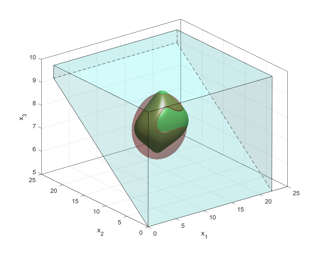
Figure 1: Invariant set for the model-based case in light red and for the data-driven case in green ($|d|\leq 10^{-3}$, $T=1000$). The safe set in light blue highlights that the two invariant sets comply with safety constraints.

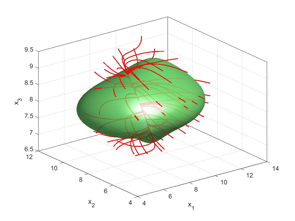
Figure 2: To show that the invariant set $\mathcal{I}$ (green) given by (38) is invariant, we simulate the closed loop system with initial conditions slightly outside $\mathcal{I}$, close to the boundary. All simulated trajectories (red) never leave the set after entering it.

6 Conclusions

In this work we addressed the problem of enforcing invariance for a polynomial system based on data. We assumed that data are corrupted by noise, whose nature and characteristic are unknown except for an (instantaneous) bound. The presence of noise resulted then in a set of dynamics consistent with data, which we over-approximated via matrix ellipsoids and took into account in the design. Our solution provided a data-dependent SOS optimization program to obtain a state feedback controller and an invariant set for the closed loop system and we optimized the size of the invariant set under the constraint that it remains contained in a user-defined safety set. Finally, we tested our data-driven algorithm on a platooning example where we showed that, for a reasonable noise level, our solution compares well with the case of perfect model knowledge. In this work we focused on enforcing invariance around one predefined state and it would be interesting to extend our data-driven design for safety around a prescribed trajectory in future research.

References

- [1] A. A. Ahmadi. Non-monotonic Lyapunov functions for stability of nonlinear and switched systems: theory and computation. Master’s thesis, Mass. Inst. Tech., 2008.
- [2] A. A. Ahmadi and B. El Khadir. Learning dynamical systems with side information. In Proc. 2nd Conf. Learn. Dynam. Contr., 2020.
- [3] A. Alan, A.J. Taylor, C. R. He, G. Orosz, and A. D. Ames. Safe controller synthesis with tunable input-to-state safe control barrier functions. IEEE Contr. Sys. Lett., 2021.
- [4] J. P. Aubin, A. M. Bayen, and P. Saint-Pierre. Viability theory: new directions. Springer, 2011.
- [5] A. Bisoffi, C. De Persis, and P. Tesi. Data-driven control via Petersen’s lemma. arXiv preprint available at https://arxiv.org/abs/2109.12175.
- [6] A. Bisoffi, C. De Persis, and P. Tesi. Controller design for robust invariance from noisy data. arXiv preprint available at https://arxiv.org/abs/2007.13181, 2020.
- [7] A. Bisoffi, C. De Persis, and P. Tesi. Trade-offs in learning controllers from noisy data. Sys. & Contr. Lett., 154:104985, 2021.
- [8] F. Blanchini. Set invariance in control. Automatica, 35(11):1747–1767, 1999.
- [9] S. Boyd, L. El Ghaoui, E. Feron, and V. Balakrishnan. Linear matrix inequalities in system and control theory. SIAM, 1994.
- [10] S. I. Chernyshenko, P. Goulart, D. Huang, and A. Papachristodoulou. Polynomial sum of squares in fluid dynamics: a review with a look ahead. Phil. Trans. Royal Soc. A: Mathem., Phys. Eng. Sciences, 372(2020), 2014.
- [11] G. Chesi. LMI techniques for optimization over polynomials in control: a survey. IEEE Trans. Autom. Contr., 55(11):2500–2510, 2010.
- [12] J. Coulson, J. Lygeros, and F. Dörfler. Data-enabled predictive control: In the shallows of the DeePC. In Proc. Eur. Contr. Conf., 2019.
- [13] T. Dai and M. Sznaier. A moments based approach to designing MIMO data driven controllers for switched systems. In IEEE Conf. Dec. Contr., 2018.
- [14] T. Dai and M. Sznaier. A semi-algebraic optimization approach to data-driven control of continuous-time nonlinear systems. IEEE Contr. Sys. Lett., 5(2):487–492, 2021.
- [15] C. De Persis and P. Tesi. Formulas for data-driven control: Stabilization, optimality, and robustness. IEEE Trans. Autom. Contr., 65(3):909–924, 2019.
- [16] K. Garg and D. Panagou. Robust control barrier and control Lyapunov functions with fixed-time convergence guarantees. In Proc. Amer. Contr. Conf., 2021.
- [17] E. Garone, S. Di Cairano, and I. Kolmanovsky. Reference and command governors for systems with constraints: A survey on theory and applications. Automatica, 75:306–328, 2017.
- [18] M. Guo, C. De Persis, and P. Tesi. Data-driven stabilization of nonlinear polynomial systems with noisy data. IEEE Trans. Autom. Contr., 2021. Early access.
- [19] H. Hjalmarsson and L. Ljung. A discussion of “unknown-but-bounded” disturbances in system identification. In Proc. IEEE Conf. Dec. Contr., 1993.
- [20] M. Jankovic. Robust control barrier functions for constrained stabilization of nonlinear systems. Automatica, 96:359–367, 2018.
- [21] Z. Jarvis-Wloszek, R. Feeley, W. Tan, K. Sun, and A. Packard. Control applications of sum of squares programming. In Positive Polynomials in Control, pages 3–22. Springer, 2005.
- [22] M. V. Lakshmi, G. Fantuzzi, J. D. Fernández-Caballero, Y. Hwang, and S. I. Chernyshenko. Finding extremal periodic orbits with polynomial optimization, with application to a nine-mode model of shear flow. SIAM J. Appl. Dyn. Sys., 19(2):763–787, 2020.
- [23] J. Löfberg. YALMIP: A toolbox for modeling and optimization in MATLAB. In Proc. IEEE Int. Symp. Comp. Aid. Contr. Sys. Des., 2004.
- [24] J. Löfberg. Pre- and post-processing sum-of-squares programs in practice. IEEE Trans. Autom. Contr., 54(5):1007–1011, 2009.
- [25] B. T. Lopez, J.J.E. Slotine, and J. P. How. Robust adaptive control barrier functions: An adaptive and data-driven approach to safety. IEEE Contr. Sys. Lett., 5(3):1031–1036, 2020.
- [26] A. Majumdar, A. A. Ahmadi, and R. Tedrake. Control design along trajectories with sums of squares programming. In Proc. IEEE Int. Conf. Rob. Autom., 2013.
- [27] I. Markovsky and P. Rapisarda. Data-driven simulation and control. Int. J. Contr., 81(12):1946–1959, 2008.
- [28] M. Milanese and C. Novara. Set membership identification of nonlinear systems. Automatica, 40(6):957–975, 2004.
- [29] M. Nagumo. Über die Lage der Integralkurven gewöhnlicher Differentialgleichungen. Proc. Physico-Mathem. Soc. of Japan, 3rd Ser., 1942.
- [30] A. Papachristodoulou and S. Prajna. A tutorial on sum of squares techniques for systems analysis. In Proc. Amer. Contr. Conf., 2005.
- [31] P. A. Parrilo. Structured semidefinite programs and semialgebraic geometry methods in robustness and optimization. PhD thesis, Cal. Inst. Tech., 2000.
- [32] S. Prajna and A. Jadbabaie. Safety verification of hybrid systems using barrier certificates. In Proc. Int. Worksh. Hybr. Sys. Comp. Contr., 2004.
- [33] W. Shaw Cortez and D. V. Dimarogonas. Safe-by-design control for Euler-Lagrange systems. arXiv preprint arXiv:2009.03767, 2021.
- [34] W. Tan and A. Packard. Stability region analysis using polynomial and composite polynomial Lyapunov functions and sum-of-squares programming. IEEE Trans. Autom. Contr., 53(2):565–571, 2008.
- [35] K. P. Wabersich and M. N. Zeilinger. Scalable synthesis of safety certificates from data with application to learning-based control. In Proc. Eur. Contr. Conf., 2018.
- [36] P. Wieland and F. Allgöwer. Constructive safety using control barrier functions. IFAC Proc. Vol., 2007.
- [37] J. C. Willems, P. Rapisarda, I. Markovsky, and B.L.M. De Moor. A note on persistency of excitation. Sys. & Contr. Lett., 54(4):325–329, 2005.
- [38] J. Wolff and M. Buss. Invariance control design for constrained nonlinear systems. In IFAC Proc. Vol., 2005.
- [39] X. Xu, J. W. Grizzle, P. Tabuada, and A. D. Ames. Correctness guarantees for the composition of lane keeping and adaptive cruise control. IEEE Trans. Autom. Science Eng., 15(3):1216–1229, 2017.
- [40] X. Xu, P. Tabuada, J. W. Grizzle, and A. D. Ames. Robustness of control barrier functions for safety critical control. In IFAC-PapersOnLine, 2015.
- [41] Y. Zheng, G. Fantuzzi, and A. Papachristodoulou. Chordal and factor-width decompositions for scalable semidefinite and polynomial optimization. Ann. Rev. Contr., 2021.