Formal verification of unknown dynamical systems via Gaussian process regression

Abstract

Leveraging autonomous systems in safety-critical scenarios requires verifying their behaviors in the presence of uncertainties and black-box components that influence the system dynamics. In this article, we develop a framework for verifying partially-observable, discrete-time dynamical systems with unmodelled dynamics against temporal logic specifications from a given input-output dataset. The verification framework employs Gaussian process (GP) regression to learn the unknown dynamics from the dataset and abstract the continuous-space system as a finite-state, uncertain Markov decision process (MDP). This abstraction relies on space discretization and transition probability intervals that capture the uncertainty due to the error in GP regression by using reproducible kernel Hilbert space analysis as well as the uncertainty induced by discretization. The framework utilizes existing model checking tools for verification of the uncertain MDP abstraction against a given temporal logic specification. We establish the correctness of extending the verification results on the abstraction to the underlying partially-observable system. We show that the computational complexity of the framework is polynomial in the size of the dataset and discrete abstraction. The complexity analysis illustrates a trade-off between the quality of the verification results and the computational burden to handle larger datasets and finer abstractions. Finally, we demonstrate the efficacy of our learning and verification framework on several case studies with linear, nonlinear, and switched dynamical systems.

[Boulder]organization=Smead Aerospace Engineering Sciences, University of Colorado, Boulder,addressline=3775 Discovery Dr, city=Boulder, state=CO, postcode=80305, country=USA [Delft]organization=Delft Center for Systems and Control (DCSC), TU Delft,addressline=Mekelweg 5, city=Delft, postcode=2628 CD, country=Netherlands

1 Introduction

Recent advances in technology have led to a rapid growth of autonomous systems operating in safety-critical domains. Examples include self-driving vehicles, unmanned aircraft, and surgical robotics. As these systems are given such delicate roles, it is essential to provide guarantees on their performance. To address this need, formal verification offers a powerful framework with rigorous analysis techniques [15, 4], which are traditionally model-based. An accurate dynamics model for an autonomous system, however, may be unavailable due to, e.g., black-box components, or so complex that existing verification tools cannot handle. To deal with such shortcomings, machine learning offers capable methods that can identify models solely from data. While eliminating the need for an accurate model, these learning methods often lack quantified guarantees with respect to the latent system [24]. The gap between model-based and data-driven approaches is in fact the key challenge in verifiable autonomy. This work focuses on this challenge and aims to develop a data-driven verification method that can provide formal guarantees for systems with unmodelled dynamics.

Formal verification of continuous control systems has been widely studied, e.g., [48, 7, 17, 30, 43, 32, 33]. These methods are typically based on model checking algorithms [15, 4], which check whether a (simple) finite model satisfies a given specification. The specification language is usually a form of temporal logic, which provides rich expressivity. Specifically, linear temporal logic (LTL) and computation tree logic (CTL) are often employed for deterministic systems, and their probabilistic counterparts, probabilistic LTL and probabilistic CTL (PCTL) are used for stochastic systems [15, 4]. To bridge the gap between continuous and discrete domains, an abstraction, which is a finite representation of the continuous control system, with a simulation relation [18] is constructed. The abstraction is in the form of a finite transition system if the latent system is deterministic [7] or a finite Markov process if the latent system is stochastic [31, 13, 33]. The resulting frameworks admit strong formal guarantees. Nevertheless, these frameworks are model-based and cannot be employed for analysis of systems with unknown models.

Machine learning has emerged as a powerful force for regressing unknown functions given a dataset. Nonparametric methods such as Gaussian process (GP) regression are winning favor for analyzing black-box systems due to their predictive power, uncertainty quantification, and ease of use [42, 45]. By conditioning a prior GP on a dataset generated by a latent function, the regression returns a posterior GP that includes the maximum a posteriori estimate of the function. The main challenge in using machine learning for verification is a proper treatment of the learning uncertainty. If this uncertainty is not formally characterized, the guarantees generated using the learned model are not applicable to the latent system. For unknown linear dynamics, specifically, techniques such as Bayesian inference along with trajectory sampling and chance-constrained have been explored for behavior and stability analysis [20, 29]. For more general systems, estimation methods such as piecewise-polynomial functions and GPs coupled with barrier functions have been developed [2, 28]. While these approaches provide means for analysis, they often lack the required formalism of the learning uncertainty or do not allow the use of full power of model-based frameworks.

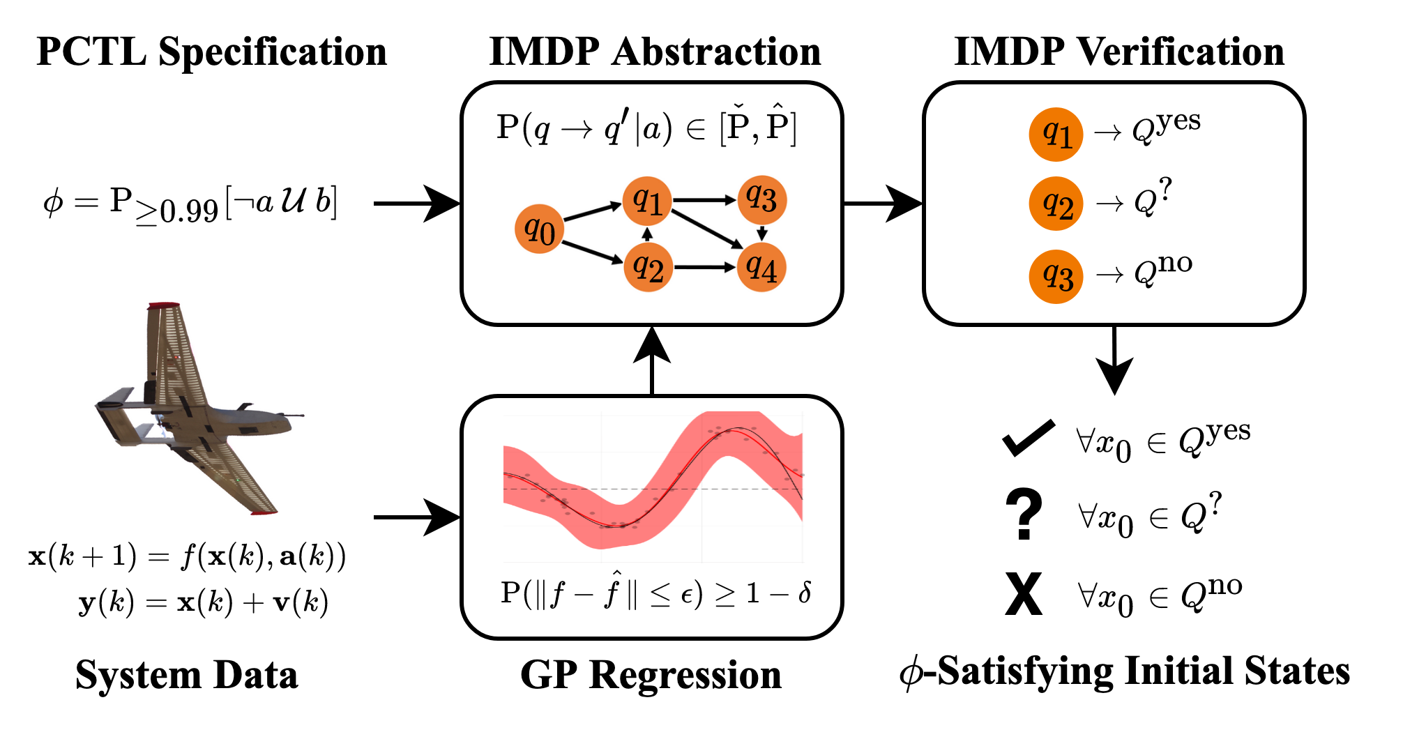
Figure 1: Overview of our learning-based, formal verification framework.

This article details an end-to-end data-driven verification framework that enables the use of off-the-shelf model-based verification tools and provides the required formalism to extend the guarantees to the latent system. An overview of the framework is shown in Figure 1. Given a noisy input-output dataset of the latent system and a temporal logic specification (LTL or PCTL formula), the framework produces verification results in the form of three sets of initial states: $Q^{\text{yes}}$, $Q^{\text{?}}$, $Q^{\text{no}}$, from which the system is guaranteed to fully, possibly, and never satisfy the specification, respectively.

Beginning with the dataset, the framework learns the dynamics via GP regression and formally quantifies the distance between the learned model and the latent system. For this step, we build on the GP regression error analysis in [45] and derive formal bounds for all of its terms. Then, it constructs a finite-state, uncertain Markov decision process (MDP) abstraction, which includes probabilistic bounds for every possible behavior of the system. Next, it uses an existing model checking tool to verify the abstraction against a given PCTL or LTL formula. Here, we specifically focus on PCTL formulas since a model checking tool for uncertain MDPs is readily available [32]. Finally, the framework closes the verification loop by mapping the resulting guarantees to the latent system.

The main contribution of this work is a data-driven formal verification framework for unknown dynamical systems. The novelties include:

1. formalization of the GP regression error bound in [45] by deriving bounds for its challenging constants,

2. an abstraction procedure including derivation of optimal transition probability bounds,

3. a proof of correctness of the final verification results for the latent system, and

4. an illustration of the framework on several case studies with linear, nonlinear, and switched dynamical systems as well as empirical analysis of parameter trade-offs.

1.1 Related Work

Recently, there has been a surge in applying formal verification methods with machine learning components in the loop [41, 52]. These applications have ranged from the explicit safety verification of actions dictated by neural network controllers [25], to using model-based checking to verify the properties of a fault-detection model using multilayer perceptron networks [44], to learning a system using machine learning regression from noisy measurements and performing rigorous safety verification [26, 27, 51]. We begin with a brief overview of model checking for verification, and then discuss its application to learning-based approaches for dynamic systems.

Formal verification generates behavior guarantees for a system with respect to a performance specification expressed in a formal logic [15, 6]. Applying verification to a continuous-space system often depends on constructing a finite-state abstraction with a simulation relation with the original system [18, 31] and employment of a model checking tool. For a fully known continuous stochastic system, an uncertain abstraction model defined as Interval-valued MDP (IMDP), which defines a space of MDPs, can be constructed and model checked against PCTL specifications [31, 32, 35, 36, 37]. For a system with unknown dynamics and complex uncertainty distributions, however, it is not clear how to construct such an abstraction. In this work, we focus on IMDPs as abstraction models due to their capability of incorporating multiple types of model uncertainties as well as their existing model checking tools [21, 22, 32].

To reason about a latent system, data-driven methods use a static dataset or active data collection. Data-driven modelling and verification have been used to check parameterized, linear time-invariant systems subject to performance specifications [20], and to perform verification of stochastic linear systems with unmodelled errors [53]. Extending to nonlinear systems is more challenging when rigorous guarantees are desired. In the absence of structural assumptions, the stability of black-box linear and nonlinear systems has been studied in the context of probabilistic invariant sets with confidence bounds that depend on a sample of system trajectories [29, 50]. The probability bounds depend solely on the number of samples, and cannot be used for systems with partial observability as we consider in this paper.

GP regression is widely employed for functional regression from noisy measurements due to its universal approximation power and probabilistic error results [42]. Of note, GP regression has been used to learn maximal invariant sets in the reinforcement learning scenario [3, 47, 8, 9] and for runtime control and verification of dynamic systems [23, 53]. Each of the previous studies considers the safety problem with a simple objective, whereas our focus is on verification against complex (temporal logic) specifications. Control barrier functions have been applied to a system with polynomial dynamics learned via GP regression for control generation subject to LTL specifications [28], although the structural assumption is restrictive and there is no guarantee that a control barrier function can be found if one exists. In addition, many methods that use GPs employ parameter approximations, e.g., Reproducing Kernel Hilbert Space (RKHS) constants, that subject final guarantees to the approximation correctness. We employ GPs as the learning model of the dynamics and overcome the approximation errors by deriving formal bounds for the parameters, leading to formal guarantees.

2 Problem Formulation

We consider a partially-observable, controlled discrete-time process given by

$$\begin{split}\textnormal{{x}}(k+1)&=f(\textnormal{{x}}(k),\textnormal{{a}}(k))\\ \textnormal{{y}}(k)&=\textnormal{{x}}(k)+\mathbf{v}(k),\end{split}$$ (1)

$$k\in\mathbb{N},\;\;\;\textnormal{{x}}(k)\in\mathbb{R}^{n},\;\;\;\textnormal{{a}}(k)\in A,\;\;\;\textnormal{{y}}(k)\in\mathbb{R}^{n},\;\;\;$$

where $A=\{a_{1},\dots,a_{|A|}\}$ is a finite set of actions, $f\mathrel{\mathop{\mathchar 58\relax}}\mathbb{R}^{n}\times\,A\rightarrow\mathbb{R}^{n}$ is a (possibly non-linear) function that is unknown, y is a noisy measurement of state x with additive noise $\mathbf{v}(k)$, a random variable with probability density function $p_{\mathbf{v}}$. We assume that $p_{\mathbf{v}}$ is a stationary sub-Gaussian distribution independent of the value of $\mathbf{v}$ at the previous time steps. Intuitively, y is a stochastic process whose behavior depends on the latent process x, which itself is driven by actions in $A$.

The evolution of Process (1) is described using trajectories of the states and measurements. A finite state trajectory up to step $k$ is a sequence of state-action pairs denoted by $\omega_{\textnormal{{x}}}^{k}=x_{0}\xrightarrow{a_{0}}x_{1}\xrightarrow{a_{1}}\ldots\xrightarrow{a_{k-1}}x_{k}$. The state trajectory $\omega_{\textnormal{{x}}}^{k}$ induces a measurement (or observation) trajectory $\omega_{\textnormal{{y}}}^{k}=y_{0}\xrightarrow{a_{0}}y_{1}\xrightarrow{a_{1}}\ldots\xrightarrow{a_{k-1}}y_{k}$ via the measurement noise process. We denote infinite-length state and measurement trajectories by $\omega_{\textnormal{{x}}}$ and $\omega_{\textnormal{{y}}}$ and the set of all state and measurement trajectories by $\Omega_{x}$ and $\Omega_{y}$, respectively. Further, we use $\omega_{x}(i)$ and $\omega_{y}(i)$ to denote the $i$-th elements of a state and measurement trajectory, respectively.

2.1 Probability Measure

We assume that the action at time $k+1$ is chosen by a control strategy $\pi_{\mathbf{y}}\mathrel{\mathop{\mathchar 58\relax}}\Omega_{y}^{k}\to A$ based on the measurement trajectory up to time $k$. This action is stochastic due to the noise process $\mathbf{v},$ which induces a probability distribution over the trajectories of the latent process x. In particular, given a fixed initial condition $x_{0}\in\mathbb{R}^{n}$ and a strategy $\pi_{\mathbf{y}}$, we denote with $\omega_{y,v_{0},\ldots,v_{k}}^{k,\pi_{\mathbf{y}},x_{{0}}}$ the measurement trajectory with noise at time $0\leq i\leq k$ fixed to $v_{i}$ and relative to the inducing state trajectory $\Omega^{k}_{x}$ such that $\Omega^{k}_{x}(0)=x_{0}$. We can then define the probability space $(\Omega_{x}^{k},\mathcal{B}(\Omega_{x}^{k}),\textnormal{P}),$ where $\mathcal{B}(\Omega_{x}^{k})$ is the $\sigma$-algebra on $\Omega_{x}^{k}$ generated by the product topology, and P is a probability measure on the sets in $\mathcal{B}(\Omega_{x}^{k})$ such that for a set $X\subset\mathbb{R}^{n}$ [10]:

$$\textnormal{P}(\omega_{\mathbf{x}}(0)\in X)=\mathbf{1}_{X}(x_{0}),$$

$$\textnormal{P}(\omega_{\mathbf{x}}(k)\in X\mid\omega_{\mathbf{x}}(0)=x_{0})=\int...\int T\big{(}X\mid x,\pi_{\mathbf{y}}(\omega_{y,v_{0},\ldots,v_{k-1}}^{k-1,\pi_{\mathbf{y}},x_{0}})\big{)}$$

$$\hskip 128.0374ptp_{\mathbf{v}}(v_{k-1})\ldots p_{\mathbf{v}}(v_{0})dv_{k-1}\ldots dv_{0},$$

where

$$\mathbf{1}_{X}(x)=\begin{cases}1&\text{if }x\in X\\ 0&\text{otherwise}\end{cases}$$

is the indicator function, and

$$T(X\mid x,a)=\textnormal{P}(\omega_{\textnormal{{x}}}(k)\in X\mid\omega_{\textnormal{{x}}}(k-1)=x,\textnormal{{a}}_{k-1}=a)$$ (2)

is the transition kernel defining the single step probabilities for Process (1). In what follows, we call $t(\bar{x}\mid x,a)$ the density function associated to the transition kernel, i.e.,

$$T(X\mid x,a)=\int_{X}t(\bar{x}\mid x,a)d\bar{x}.$$

Intuitively, P is defined by marginalizing $T$ over all possible observation trajectories. Note that as the initial condition $x_{0}$ is fixed, the marginalization is over the distribution of the noise up to time $k-1.$ We remark that P is also well defined for $k=\infty$ by the Ionescu-Tulcea extension theorem [1].

The above definition of P implies that if $f$ were known, the transition probabilities of Process (1) are Markov and deterministic once the action is known. However, we stress that, even in the case where $a$ is known, the exact computation of the above probabilities is infeasible in general as $f$ is unknown. Next, we introduce continuity assumptions that allow us to estimate $f$ from a dataset of noisy observations and consequently to compute bounds on the transition kernel $T$.

2.2 Continuity Assumption

Taking function $f$ as completely unknown leads to an ill-posed problem. Hence, we employ the following standard assumption [45], [14], which constrains $f$ to be a well-behaved analytical function on a compact (closed and bounded) set.

Assumption 1 (RKHS Continuity).

For a compact set $X\subset\mathbb{R}^{n}$, let $\kappa\mathrel{\mathop{\mathchar 58\relax}}\mathbb{R}^{n}\times\mathbb{R}^{n}\to\mathbb{R}$ be a given kernel and $\mathcal{H}_{\kappa}(X)$ the reproducing kernel Hilbert space (RKHS) of functions over $X$ corresponding to $\kappa$ with norm $\|\cdot\|_{\kappa}$ [45]. Then, for each $a\in A$ and $i\in\{1,\ldots,n\},$ $f^{(i)}(\cdot,a)\in\mathcal{H}_{\kappa}(X)$ and for a constant $B_{i}>0,$ $\|f^{(i)}(\cdot,a)\|_{\kappa}\leq B_{i}$, where $f^{(i)}$ is the $i$-th component of $f$.

Although Assumption 1 limits $f$ to a class of analytical functions, it is not overly restrictive as we can choose $\kappa$ such that $\mathcal{H}_{\kappa}$ is dense in the space of continuous functions [46]. For instance, this holds for the widely-used squared exponential (radial basis) kernel function [42]. This assumption allows us to use GP regression to estimate $f$ and leverage error results as we detail in Section 3.1.

Remark 1.

The model for Process (1) considered in this work is quite general and includes autonomous dynamical systems that operate under a given control strategy (typically black-box feedback controller, e.g., neural network controller) as long as Assumption 1 is satisfied. In that case, Process (1) becomes a closed-loop system and the unknown function $f$ is simply dependent only on state x (no longer dependant on action).

2.3 PCTL Specifications

We are interested in the behavior of the latent process x as defined in (1) over regions of interest $\mathcal{R}=\{r_{1},\dots,r_{|\mathcal{R}|}\}$ with $r_{i}\subset\mathbb{R}^{n}$. For example, these regions may indicate target sets that should be visited or unsafe sets that must be avoided both in the sense of physical obstacles and state constraints (e.g., velocity limits). In order to define properties over $\mathcal{R}$, for a given state $x$ and region $r_{i}$, we define an atomic proposition $\mathfrak{p}_{i}$ to be true ($\top$) if $x\in r_{i}$, and otherwise false ($\bot$). The set of atomic propositions is given by $AP$, and the label function $L\mathrel{\mathop{\mathchar 58\relax}}\mathbb{R}^{n}\to 2^{AP}$ returns the set of atomic propositions that are true at each state.

Probabilistic computational tree logic (PCTL) [5] is a formal language that allows for the expression of complex behaviors of stochastic systems. We begin by defining the syntax and semantics of PCTL specifications.

Definition 1 (PCTL Syntax).

Formulas in PCTL are recursively defined over the set of atomic propositions $AP$ in the following manner:

$$\text{State Formula}\quad\phi \coloneqq\top\;|\;\mathfrak{p}\;|\;\neg\phi\;|\;\phi\wedge\phi\;|\;\textnormal{P}_{\bowtie p}[\psi]$$

$$\text{Path Formula}\quad\psi \coloneqq\mathcal{X}\phi\;|\;\phi\,\mathcal{U}^{\leq k}\phi\;|\;\phi\,\mathcal{U}\phi$$

where $\mathfrak{p}\in AP$, $\neg$ is the negation operator, $\wedge$ is the conjunction operator, $\textnormal{P}_{\bowtie p}$ is the probabilistic operator, $\bowtie\in\{\leq,<,\geq,>\}$ is a relation placeholder, and $p\in[0,1]$. The temporal operators are the $\mathcal{X}$ (Next), $\mathcal{U}^{\leq k}$ (Bounded-Until) with respect to time step $k\in\mathbb{N}$, and $\mathcal{U}$ (Until).

Definition 2 (PCTL Semantics).

The satisfaction relation $\models$ is defined inductively as follows. For state formulas,

• $x\models\top$ for all $x\in\mathbb{R}^{n}$;

• $x\models\mathfrak{p}\iff\mathfrak{p}\in L(x)$;

• $x\models(\phi_{1}\wedge\phi_{2})\iff(x\models\phi_{1})\wedge(x\models\phi_{2})$;

• $x\models\neg\phi\iff x\nvDash\phi$;

• $x\models\textnormal{P}_{\bowtie p}[\psi]\iff p^{x}(\psi)\bowtie p$, where $p^{x}(\psi)$ is the probability that all infinite trajectories initialized at $x$ satisfy $\psi$.

For a state trajectory $\omega_{\textnormal{{x}}}$, the satisfaction relation $\models$ for path formulas is defined as:

• $\omega_{\textnormal{{x}}}\models\mathcal{X}\phi\iff\omega_{\textnormal{{x}}}(1)\models\phi$;

• $\omega_{\textnormal{{x}}}\models\phi_{1}\mathcal{U}^{\leq k}\phi_{2}\iff\exists i\leq k$ s.t. $\omega_{\textnormal{{x}}}(i)\models\phi_{2}\wedge\omega_{\textnormal{{x}}}(j)\models\phi_{1}\;\forall j\in[0,i)$;

• $\omega_{\textnormal{{x}}}\models\phi_{1}\mathcal{U}\phi_{2}\iff\exists i\geq 0$ s.t. $\omega_{\textnormal{{x}}}(i)\models\phi_{2}\wedge\omega_{\textnormal{{x}}}(j)\models\phi_{1}\;\forall j\in[0,i)$.

The common operators bounded eventually $\mathcal{F}^{\leq k}$ and eventually $\mathcal{F}$ are defined respectively as

$$\textnormal{P}_{\bowtie p}[\mathcal{F}^{\leq k}\phi]\equiv\textnormal{P}_{\bowtie p}[\top\mathcal{U}^{\leq k}\phi],\quad\text{and}\quad\textnormal{P}_{\bowtie p}[\mathcal{F}\phi]\equiv\textnormal{P}_{\bowtie p}[\top\mathcal{U}\phi].$$

The globally operators $\mathcal{G}^{\leq k}$ and $\mathcal{G}$ are defined as

$$\textnormal{P}_{\bowtie p}[\mathcal{G}^{\leq k}\phi]\equiv\textnormal{P}_{\bar{\bowtie}1-p}[\mathcal{F}\neg\phi],\quad\text{and}\quad\textnormal{P}_{\bowtie p}[\mathcal{G}\phi]\equiv\textnormal{P}_{\bar{\bowtie}1-p}[\mathcal{F}\neg\phi],$$

where $\bar{\bowtie}$ indicates the opposite relation, i.e, $\bar{<}\equiv\;>$, $\bar{\leq}\equiv\;\geq$, $\bar{\geq}\equiv\;\leq$, and $\bar{>}\equiv\;<$.

PCTL provides a rich, expressive language to specify probabilistic properties of systems. As an example the property, “the probability of reaching the target by going through safe regions or regions, from which the probability of ending up in an unsafe set in one time step is less than 0.01, is greater or equal to 0.95” can be expressed with the PCTL formula

$$\phi=\textnormal{P}_{\geq 0.95}\big{[}\big{(}\mathfrak{p}_{\text{safe}}\vee\textnormal{P}_{<0.01}[\mathcal{X}\,\mathfrak{p}_{\text{unsafe}}]\big{)}\,\mathcal{U}\,\mathfrak{p}_{\text{target}}\big{]}.$$

2.4 Problem Statement

We are interested in verification of Process (1) against PCTL formulas. The verification problem asks whether Process (1) satisfies a PCTL formula $\phi$ under all control strategies. It can also be posed as finding the set of initial states in a compact set $X\subset\mathbb{R}^{n}$, from which Process (1) satisfies $\phi$.

In lieu of an analytical form of $f$, we assume to have a dataset $\mathrm{D}=\{(x_{i},a_{i},y_{i})\}_{i=1}^{d}$ generated by Process (1) where $y_{i}$ is the noisy measurement of $f(x_{i},a_{i})$, and $d\in\mathbb{N}^{+}$. Using this dataset, we can infer $f$ and reason about the trajectories of Process (1) (via Assumption 1). The formal statement of the problem considered in this work is as follows.

Problem 1.

Let $X\subset\mathbb{R}^{n}$ be a compact set, $\mathcal{R}$ a set of regions of interest, and $AP$ its corresponding set of atomic propositions (as defined in Section 2.3). Given a dataset $\mathrm{D}$ generated by Process (1) and a PCTL formula $\phi$ defined over $AP$, determine the initial states $X_{0}\subset X$ from which Process (1) satisfies $\phi$ without leaving $X$.

Our approach to Problem 1 is based on creating a finite abstraction of the latent process x using GP regression and checking if the abstraction satisfies $\phi$. We begin by estimating the unknown dynamics with GP regression and, by virtue of Assumption 1, we develop probabilistic error bounds on the estimate. We derive formal upper bounds on all the constants required by the bounds and compute bounds on the transition kernel in Eq. (2) over a discretization of the space $X$. Then, we construct the abstraction of Process (1) in the form of an uncertain (interval-valued) Markov decision process, which accounts for the uncertainties in the regression of $f$ and the discretization of $X$. Finally, we perform model checking on the abstraction to get sound bounds on the probability that $\mathbf{x}$ satisfying $\phi$ from any initial state.

Remark 2.

We remark that our IMDP abstraction construction is general, and hence, can be used for verification of Process (1) against properties in other specification languages such as LTL. We specifically focus on PCTL properties mainly because of the availability of its model checking tool for IMDPs [32].

3 Preliminaries

In this section, we provide a brief overview of the main concepts behind GP regression and interval MDPs, which we use to approach Problem 1.

3.1 Gaussian Process Regression

Gaussian process (GP) regression [42] aims to estimate an unknown function $\mathrm{f}\mathrel{\mathop{\mathchar 58\relax}}\mathbb{R}^{n}\to\mathbb{R}$ from a dataset $\mathrm{D}=\{(\mathrm{x}_{i},\mathrm{y}_{i})\}_{i=1}^{d}$ where $\mathrm{y}_{i}=\mathrm{f}(\mathrm{x}_{i})+\mathrm{v}_{i}$ and $\mathrm{v}_{i}$ is a sample of a normal distribution with zero mean and $\sigma_{\mathbf{v}}^{2}$ variance, denoted by $\mathrm{v}_{i}\sim\mathcal{N}(0,\sigma_{\mathbf{v}}^{2})$. The standard assumption is that $\mathrm{f}$ is a sample from a GP with zero-valued mean function and kernel function $\kappa_{0}$. Let $X$ and $Y$ be ordered vectors with all points in $\mathrm{D}$ such that $X_{i}=\mathrm{x}_{i}$ and $Y_{i}=\mathrm{y}_{i}$. Further, let $K$ denote the matrix with element $K_{i,j}=\kappa_{0}(\mathrm{x}_{i},\mathrm{x}_{j})$, $k(\mathrm{x},X)$ the vector such that $k_{i}(\mathrm{x},X)=\kappa_{0}(\mathrm{x},X_{i})$, and $k(X,\mathrm{x})$ defined accordingly. Predictions at a new input point $\mathrm{x}$ are given by the conditional distribution of the prior at $\mathrm{x}$ given $\mathrm{D}$, which is still Gaussian and with mean $\mu_{\mathrm{D}}$ and variance $\sigma_{\mathrm{D}}^{2}$ given by

$$\begin{split}&\mu_{\mathrm{D}}(\mathrm{x})=k(\mathrm{x},X)^{T}\big{(}K+\sigma_{\mathrm{v}}^{2}I\big{)}^{-1}Y\end{split}$$ (3)

$$\begin{split}&\sigma_{\mathrm{D}}^{2}(\mathrm{x})=\kappa_{0}(\mathrm{x},\mathrm{x})-k(\mathrm{x},X)^{T}\big{(}K+\sigma_{\mathrm{v}}^{2}I\big{)}^{-1}k(X,\mathrm{x})\end{split}$$ (4)

where $I$ is the identity matrix of size $d$.

In this work, we do not make the standard assumption that $f$ in Process (1) is distributed according to the prior GP. We also consider sub-Gaussian noise, which is a larger class of observation noise than Gaussian noise. Hence, we cannot directly use Eq. (LABEL:eq:post-mean) and (LABEL:eq:post-kernel) to bound the latent function. Rather, as common in the literature [45], we rely on the relationship between GP regression and the reproducing kernel Hilbert space (RKHS).

3.2 Reproducing Kernel Hilbert Spaces

Intuitively, given a GP with kernel $\kappa$, the associated reproducing kernel Hilbert space (RKHS) $\mathcal{H}_{\kappa}$ is a Hilbert space of functions composed by analytical functions that are in the span of $\kappa$ over all finite subsets of a compact set $X$. For universal kernels such as the squared exponential, the resulting RKHS is dense in the continuous functions on any compact set [39]. Under Assumption 1, the following proposition bounds the GP learning error when $f$ is a function in $\mathcal{H}_{\kappa}$, without posing any distributional assumption on $f$.

Proposition 1 ([14], Theorem 2).

Let $X$ be a compact set, $\delta\in(0,1]$, and $\mathrm{D}$ be a given dataset generated by $\mathrm{f}$. Suppose we can find $\Gamma>0$ such that the maximum information gain of $\kappa$ is bounded, i.e., $\gamma^{d}_{\kappa}\leq\Gamma$, and $B>0$ such that $\|\mathrm{f}\|_{\kappa}\leq B$. Assume that $\mathrm{v}$ is $R$-sub-Gaussian and that $\mu_{\mathrm{D}}$ and $\sigma_{\mathrm{D}}$ are found by setting $\sigma_{\mathrm{v}}^{2}=1+2/d$ and using (LABEL:eq:post-mean) and (LABEL:eq:post-kernel). Define $\beta(\delta)=(R/\sigma_{\mathrm{v}})(B+R\sqrt{2(\Gamma+1+\log{1/\delta})})$. Then, it holds that

$$\textnormal{P}\big{(}\forall x\in X,|\mu_{\mathrm{D}}(\mathrm{x})-\mathrm{f}(\mathrm{x})|\leq\beta(\delta)\sigma_{\mathrm{D}}(\mathrm{x})\big{)}\geq 1-\delta.$$ (5)

Proposition 1 assumes that the noise on the measurements is $R$-sub-Gaussian, which is more general than Gaussian noise. It depends on the constants $\|\mathrm{f}\|_{\kappa}$ and $\gamma^{d}_{\kappa}$ which have been described as challenging to deal with [34], and are often picked according to heuristics without guarantees [8, 28]. In this work, we derive formal upper bounds for each of these terms in Section 4.2.2.

3.3 Interval Markov Decision Processes

An interval Markov decision process (IMDP) is a generalization of a Markov decision process, where the transitions under each state-action pair are defined by probability intervals [19].

Definition 3 (Interval MDP).

An interval Markov decision process is a tuple $\mathcal{I}=(Q,A,\check{\textnormal{P}},\hat{\textnormal{P}},AP,L)$ where

• $Q$ is a finite set of states,

• $A$ is a finite set of actions, where $A(q)$ is the set of available actions at state $q\in Q$,

• $\check{\textnormal{P}}\mathrel{\mathop{\mathchar 58\relax}}Q\times A\times Q\to[0,1]$ is a function, where $\check{\textnormal{P}}(q,a,q^{\prime})$ defines the lower bound of the transition probability from state $q\in Q$ to state $q^{\prime}\in Q$ under action $a\in A(q)$,

• $\hat{\textnormal{P}}\mathrel{\mathop{\mathchar 58\relax}}Q\times A\times Q\to[0,1]$ is a function, where $\hat{\textnormal{P}}(q,a,q^{\prime})$ defines the upper bound of the transition probability from state $q$ to state $q^{\prime}$ under action $a\in A(q)$,

• $AP$ is a finite set of atomic propositions,

• $L\mathrel{\mathop{\mathchar 58\relax}}Q\to 2^{AP}$ is a labeling function that assigns to each state $q$ possibly several elements of $AP$.

For all $q,q^{\prime}\in Q$ and $a\in A(q)$, it holds that $\check{\textnormal{P}}(q,a,q^{\prime})\leq\hat{\textnormal{P}}(q,a,q^{\prime})$ and

$$\sum_{q^{\prime}\in Q}\check{\textnormal{P}}(q,a,q^{\prime})\leq 1\leq\sum_{q^{\prime}\in Q}\hat{\textnormal{P}}(q,a,q^{\prime}).$$

Let $\mathcal{D}(Q)$ denote the set of probability distributions over $Q$. Given $q\in Q$ and $a\in A(q)$, we call $\mathfrak{t}_{q}^{a}\in\mathcal{D}(Q)$ a feasible distribution over states reachable from $q$ under $a$ if the transition probabilities respect the intervals defined for each possible successor state $q^{\prime}$, i.e., $\check{\textnormal{P}}(q,a,q^{\prime})\leq\mathfrak{t}_{q}^{a}(q^{\prime})\leq\hat{\textnormal{P}}(q,a,q^{\prime})$. We denote the set of all feasible distributions for state $q$ and action $a$ by $\mathfrak{T}_{q}^{a}$.

A path $\omega$ of an IMDP is a sequence of states $\omega=q_{0}\xrightarrow{a_{0}}q_{1}\xrightarrow{a_{1}}q_{2}\xrightarrow{a_{2}}\ldots$ such that $a_{i}\in A(q_{i})$ and $\hat{\textnormal{P}}(q_{i},a_{i},\allowbreak{q_{i+1}})>0$ (i.e., transitioning is possible) for all $i\in\mathbb{N}$. We denote the last state of a finite path $\omega^{\mathrm{fin}}$ by $\textit{last}(\omega^{\mathrm{fin}})$ and the set of all finite and infinite paths by $\mathit{Paths}^{\mathrm{fin}}$ and $\mathit{Paths}$, respectively. Actions taken by the IMDP are determined by a choice of strategy $\pi$ which is defined below.

Definition 4 (Strategy).

A strategy $\pi$ of an IMDP $\mathcal{I}$ is a function $\pi\mathrel{\mathop{\mathchar 58\relax}}\mathit{Paths}^{\mathrm{fin}}\to A$ that maps a finite path $\omega^{\mathrm{fin}}$ of $\mathcal{I}$ onto an action in $A$. The set of all strategies is denoted by $\Pi$.

Once an action is chosen according to a strategy, a feasible distribution needs to be chosen from $\mathfrak{T}_{q}^{a}$ to enable a transition to the next state. This task falls on the adversary function $\theta$ as defined below.

Definition 5 (Adversary).

Given an IMDP $\mathcal{I}$, an adversary is a function $\theta\mathrel{\mathop{\mathchar 58\relax}}\mathit{Paths}^{\mathrm{fin}}\times A\rightarrow\mathcal{D}(Q)$ that, for each finite path $\omega^{\mathrm{fin}}\in\mathit{Paths}^{\mathrm{fin}}$ and action $a\in A(\textit{last}(\omega^{\mathrm{fin}}))$, chooses a feasible distribution $\mathfrak{t}_{q}^{a}\in\mathfrak{T}_{\textit{last}(\omega^{\mathrm{fin}})}^{a}$. The set of all adversaries is denoted by $\Theta$.

Once a strategy is selected, the IMDP becomes an interval Markov chain – further, choosing an adversary results in a standard Markov chain. Hence, given a strategy and an adversary, a probability measure can be defined on the paths of the IMDP via the probability of paths on the resulting Markov chain [32].

In the next section, we show that by appropriate construction of an IMDP abstraction for Process (1) through careful consideration of the transition kernel (Eq. $\eqref{eq:transition-kernel}$) and the regression error (Eq. (5)), the probability measures calculated from verifying the IMDP against a PCTL formula capture the true probability of Process (1) satisfying the formula.

4 IMDP Abstraction

To solve Problem 1, we begin by constructing a finite abstraction of Process (1) in the form of an IMDP that captures the state evolution of the system under known actions. This involves partitioning the set $X$ into discrete regions and determining the transition probability intervals between each pair of discrete regions under each action to account for the uncertainty induced by the learning and discretization processes. Although the IMDP does not capture the partial observability of Process (1), as we show in Section 5, it is sufficient for solving Problem 1.

4.1 IMDP States and Actions

In the first step of the abstraction, set $X$ is discretized into a finite set of non-overlapping regions $Q_{X}$ such that

$$\bigcup_{q\in Q_{X}}\leavevmode\nobreak\ q=X.$$

Also, the discretization must maintain consistent labelling with the regions of interest $\mathcal{R}=\{r_{i}\}_{i=1}^{|\mathcal{R}|}$ where $r_{i}\subseteq X$, i.e., (with an abuse of the notation of $L$),

$$L(q)=L(r_{i})\quad\text{ iff }\quad L(x)=L(r_{i})\;\;\forall x\in q.$$

To ensure this consistency, the regions of interest are used as the foundation of the discretization. Then, we define

$$Q=Q_{X}\cup\{q_{\bar{X}}\},\quad\text{ where }\quad q_{\bar{X}}=\mathbb{R}^{n}\setminus X.$$

The regions in $Q$ are associated with the states of the IMDP, and with an abuse of notation, $q\in Q$ indicates both a state of the IMDP and the associated discrete region. Finally, the IMDP action space is set to the action set $A$ of Process (1).

4.2 Transition Probability Bounds

To complete the construction of the IMDP abstraction of Process (1), the transition probability bounds on the IMDP should be selected such that

$$\check{\textnormal{P}}(q,a,q^{\prime}) \leq\min_{x\in q}T(q^{\prime}\mid x,a),$$

$$\hat{\textnormal{P}}(q,a,q^{\prime}) \geq\max_{x\in q}T(q^{\prime}\mid x,a)$$

for all $q,q^{\prime}\in Q$ and action $a\in A$. The bounds on the transition kernel $T$ must account for the probabilistic error and discretization uncertainty. We use the learned dynamics and regression errors to derive these bounds for every $(q,a,q^{\prime})$ tuple.

4.2.1 IMDP State Images and Regression Error

We perform GP regression using the given dataset $\mathrm{D}$ and analyze the evolution of each IMDP state under the learned dynamics. In addition, the associated learning error is quantified using Proposition 1.

Each output component of the dynamics under an action is estimated by a separate GP, making a total of $n\,|A|$ regressions. Let $\mu^{(i)}_{a,\mathrm{D}}(x)$ and $\sigma^{(i)}_{a,\mathrm{D}}(x)$ respectively denote the posterior mean and covariance functions for the $i$-th output component under action $a$ obtained via GP regression. These GPs are used to evolve $q$ under action $a$, defined by

$$Im(q,a)=\big{\{}\mu^{(i)}_{a,\mathrm{D}}(x)\mid x\in q,\;i\in[1,n]\big{\}},$$

which describes the evolution of all $x\in q$.

The worst-case regression error is

$$e^{(i)}(q,a)=\sup_{x\in q}|\mu^{(i)}_{a,\mathrm{D}}(x)-f^{(i)}(x,a)|,$$ (6)

which provides an error upper-bound for all continuous states $x\in q$. To use Proposition 1 for probabilistic reasoning on this worst-case error, the supremum of the posterior covariance in $q$ denoted by

$$\overline{\sigma}^{(i)}_{a,\mathrm{D}}(q)=\sup_{x\in q}\sigma^{(i)}_{a,\mathrm{D}}(x)$$

is used. Both the posterior image and covariance supremum can be calculated for each IMDP state using GP interval bounding as in  [11]. Then, Proposition 1 is applied with a scalar $\epsilon^{(i)}\geq 0$,

$$\textnormal{P}\big{(}e^{(i)}(q,a)\leq\epsilon^{(i)}\big{)}\geq 1-\delta$$ (7)

where $\delta$ satisfies $\epsilon^{(i)}=\beta(\delta)\overline{\sigma}^{(i)}_{a,\mathrm{D}}(q)$.

4.2.2 Bounds on the RKHS Parameters

The computation of $\textnormal{P}\big{(}e^{(i)}(q,a)\leq\epsilon^{(i)}\big{)}$ via Proposition 1 requires two constants: the RKHS norm $\|f^{(i)}\|_{\kappa}$ and information gain $\gamma^{d}_{\kappa}$. In this section, we provide formal upper bounds for these constants.

Proposition 2 (RKHS Norm Bound).

Let $f^{(i)}\in\mathcal{H}$ where $\mathcal{H}$ is the RKHS defined by the kernel function $\kappa$. Then

$$\|f^{(i)}\|_{\kappa}\leq\frac{\sup_{x\in X}|f^{(i)}(x)|}{\inf_{x,x^{\prime}\in X}\kappa(x,x^{\prime})^{\frac{1}{2}}}$$ (8)

for all $x,x^{\prime}\in X$.

The proof is provided in A, which relies on the relationship between the RKHS norm and the kernel function.

Proposition 2 shows that the RKHS norm of a function can be over-approximated by the quotient of the supremum of the function and the infimum of the kernel function on a compact set. Note that Eq. (8) requires the square root of the kernel in the denominator. Hence, so long the chosen kernel is a positive function (e.g., squared exponential), we can compute a finite upper bound for the RKHS norm. Moreover, as $X$ is a finite-dimensional compact set, it can be straightforward to calculate bounds for the numerator in Eq. (8) as remarked below.

Remark 3.

There are several approaches for computing the numerator of Eq. (8) for a latent function $f$. As an example, using the Lipschitz constant $L_{f^{(i)}}$ of $f^{(i)}$ (or an upper bound of it), the supremum in the numerator can be bounded by

$$\sup_{x\in X}|f^{(i)}(x)|\leq\sup_{x\in X}|x^{(i)}|+L_{f^{(i)}}\text{diam}(X).$$ (9)

where $\text{diam}(X)\coloneqq\sup_{x,x^{\prime}\in X}\|x-x^{\prime}\|$ is the diameter of $X$.

For the information gain constant $\gamma^{d}_{\kappa}$, an upper bound can be found using determinant-bounding methods that rely only on the size of the dataset. In Proposition 3, below, we use Hadamard’s inequality and the fact that $K$ is a positive-definite matrix to upper bound $\gamma^{d}_{\kappa}$.

Proposition 3 (Information Gain Bound).

Let $d$ be the size of the dataset $\mathrm{D}$ and $\sigma_{\mathrm{v}}$ the parameter used for GP regression. Then, the information gain is bounded by

$$\gamma^{d}_{\kappa}\leq d\log(1+\sigma_{\mathrm{v}}^{-2}s),$$ (10)

where $s=\sup_{x\in X}k(x,x)$.

The proof is provided in B. The bound on the information gain term in Proposition 3 relies only on bounding the determinant of $K$. Hence, it can be improved by using more detailed knowledge of the kernel function, such as its spectral properties [49].

With probabilistic regression errors defined for every possible state, the transition probability bounds between each discrete state can be derived as detailed below.

4.2.3 Transitions between states in $Q_{X}$

To reason about transitions using the images of regions, the following notations are used to indicate the expansion and reduction of a region and the intersection of two regions.

Definition 6 (Region Expansion and Reduction).

Given a compact set (region) $q\subset\mathbb{R}^{n}$ and a set of $n$ scalars $c=\{c_{1},\dots,c_{n}\}$, where $c_{i}\geq 0$, the expansion of $q$ by $c$ is defined as

$$\overline{q}(c)=\{x\in\mathbb{R}^{n}\mid\exists x_{q}\in q\;\;s.t.\;\;|x_{q}^{(i)}-x^{(i)}|\leq c_{i}\\ \forall i=\{1,\dots,n\}\},$$

and the reduction of $q$ by $c$ is

$$\underline{q}(c)=\{x_{q}\in q\mid\forall x_{\partial q}\in\partial q,\;\;|x_{q}^{(i)}-x_{\partial q}^{(i)}|>c_{i}\\ \forall i=\{1,\dots,n\}\},$$

where $\partial q$ is the boundary of $q$.

The intersection between the expanded and reduced states indicate the possibility of transitioning between the states. This intersection function is defined as

$$\mathbf{1}_{V}(W)=\begin{cases}1&\text{ if }V\cap W\neq\emptyset\\ 0&\text{ otherwise }\end{cases}$$

for sets $V$ and $W$.

The following theorem presents bounds for the transition probabilities of Process (1) that account for both the regression error and induced discretization uncertainties using Proposition 1 and sound approximations using the preceding definitions.

Theorem 1.

Suppose $q,q^{\prime}\in Q_{X}$, and let $\epsilon$, $\epsilon^{\prime}\in\mathbb{R}^{n}$ be non-negative vectors. For any action $a\in A$, the transition kernel is bounded by

$$\min_{x\in q}T(q^{\prime}\mid x,a)$$

$$\quad\quad\geq\Big{(}1-\mathbf{1}_{X\setminus\underline{q}^{\prime}(\epsilon)}\big{(}Im(q,a)\big{)}\Big{)}\prod_{i=1}^{n}\textnormal{P}\Big{(}e^{(i)}(q,a)\leq\epsilon^{(i)}\Big{)},\quad\;\;$$

and

$$\max_{x\in q}T(q^{\prime}\mid x,a)$$

$$\quad\quad\leq 1-\prod_{i=1}^{n}\textnormal{P}\big{(}e^{(i)}(q,a)\leq\epsilon^{\prime(i)}\big{)}\Big{(}1-\mathbf{1}_{\overline{q}^{\prime}(\epsilon^{\prime})}\big{(}Im(q,a)\big{)}\Big{)}.$$

Proof.

The proof of Theorem 1 relies on bounding the probability of transitioning from $q$ to $q^{\prime}$ conditioned on the learning error $\epsilon$ ($\epsilon^{\prime}$) given by Eq. (7), and using the expanded (reduced) image of $q$ with $\epsilon$ ($\epsilon^{\prime}$) to find a point in $q$ that minimizes (maximizes) this bound. We provide the proof for the upper bound on $T$, and the lower bound follows analogously.

Let $q^{\prime}$ denote subsequent states of $q$, and suppose $\omega_{\textnormal{{x}}}(k)\in q$ for an arbitrary timestep $k$. The probability of transitioning to $q^{\prime}$ under action $a$ is upper-bounded beginning with transition kernel and using the law of total probability conditioned on the learning error:

$$\max_{x\in q}\textnormal{P}(\omega_{\textnormal{{x}}}(k+1)\in q^{\prime}\mid\omega_{\textnormal{{x}}}(k)=x,a)$$

$$=\max_{x\in q}\big{(}\textnormal{P}(\omega_{\textnormal{{x}}}(k+1)\in q^{\prime}\wedge e(q,a)\leq\epsilon\mid\omega_{\textnormal{{x}}}(k)=x)\;+$$

$$\quad\qquad\qquad\qquad\;\;\;\textnormal{P}(\omega_{\textnormal{{x}}}(k+1)\in q^{\prime}\wedge e(q,a)>\epsilon\mid\omega_{\textnormal{{x}}}(k)=x)\big{)}$$

$$=\max_{x\in q}\big{(}\textnormal{P}(\omega_{\textnormal{{x}}}(k+1)\in q^{\prime}\mid e(q,a)\leq\epsilon,\omega_{\textnormal{{x}}}(k)=x)\,\textnormal{P}(e(q,a)\leq\epsilon)$$

$$\quad\>\quad+\textnormal{P}(\omega_{\textnormal{{x}}}(k+1)\in q^{\prime}\mid e(q,a)>\epsilon,\omega_{\textnormal{{x}}}(k)=x)\textnormal{P}(e(q,a)>\epsilon)\big{)}$$

Next, $\textnormal{P}(\omega_{\textnormal{{x}}}(k+1)\in q^{\prime}\mid e(q,a)\leq\epsilon,\omega_{\textnormal{{x}}}(k)=x)$ is upper bounded using the intersection indicator, $\textnormal{P}(\omega_{\textnormal{{x}}}(k+1)\in q^{\prime}\mid e(q,a)>\epsilon,\omega_{\textnormal{{x}}}(k)=x)$ is upper bounded by one, and $\textnormal{P}(e(q,a)>\epsilon)$ is replaced by the equivalent $1-\textnormal{P}(e(q,a)\leq\epsilon)$:

$$\leq\max_{x\in q}\Big{(}\mathbf{1}_{\overline{q}^{\prime}}\big{(}Im(q,a)\big{)}\,\textnormal{P}(e(q,a)\leq\epsilon)+1\cdot\big{(}1-\textnormal{P}(e(q,a)\leq\epsilon)\big{)}\Big{)}$$

$$=\max_{x\in q}\Big{(}\mathbf{1}_{\overline{q}^{\prime}}\big{(}Im(q,a)\big{)}\prod_{i=1}^{n}\textnormal{P}(e^{(i)}(q,a)\leq\epsilon_{i})\,+$$

$$\quad\quad\quad\quad\quad\quad\quad\quad\quad\quad\quad\quad\quad\quad 1-\prod_{i=1}^{n}\textnormal{P}(e^{(i)}(q,a)\leq\epsilon_{i})\Big{)},$$

where the last inequality is due to fact that the components of $\mathbf{v}$ are mutually independent. Rearranging these terms, we obtain the upper bound on $T$. ∎

The width of these bounds relies on the choices of $\epsilon$ and $\epsilon^{\prime}$, which facilitate a trade-off between the learning error probabilities and intersection functions. The following proposition provides the optimal values for both $\epsilon$ and $\epsilon^{\prime}$.

Proposition 4.

Let $\partial W$ denote the boundary of a compact set $W\subset\mathbb{R}^{n}$. The distance between the upper and lower bounds in Theorem 1 is minimized if $\epsilon^{\prime}=\epsilon$ and $\epsilon$ is chosen such that for each $i\in[1,n]$,

$$\epsilon^{(i)} =\inf_{x\in\partial Im(q,a),\,x^{\prime}\in\partial q^{\prime}}|x^{(i)}-x^{\prime(i)}|.$$

The proof for Proposition 4 is provided in C.

Remark 4.

Consider the image $Im(q,a)$ and the intersection $Im(q,a)\cap q^{\prime}$. There are three possible outcomes; (1) the intersection is empty, (2) the intersection is non-empty but not equal to $Im(q,a)$, and (3) the intersection is equal to $Im(q,a)$. By examining Theorem 1, it is clear that if (2) is true, then we get trivial transition probability bounds of $[0,1]$. In this case, the choice of $\epsilon$ does not matter. If (1) is true, then the bounds are $[0,\hat{\textnormal{P}}(q,a,q^{\prime})]$ and we have an opportunity to get a non-trivial upper bound. The best upper bound is achieved by choosing large $\epsilon$ to capture more regression error, but small enough to keep the indicator function zero. This is achieved by choosing $\epsilon$ according to Proposition 4, which corresponds to minimizing the L1 norm of $x-x^{\prime}$. Finally, if (3) is true, then the bounds are $[\check{\textnormal{P}}(q,a,q^{\prime}),1]$ and the approach is similar.

4.2.4 Transitions to $q_{\bar{X}}$

Transition intervals to the unsafe state $q_{\bar{X}}$ are the complement of the transitions to the full set $X$, or

$$\check{\textnormal{P}}(q,a,q_{\bar{X}}) =1-\hat{\textnormal{P}}(q,a,X)$$

$$\hat{\textnormal{P}}(q,a,q_{\bar{X}}) =1-\check{\textnormal{P}}(q,a,X)$$

where $\check{\textnormal{P}}(q,a,X)$ and $\hat{\textnormal{P}}(q,a,X)$ are calculated with Theorem 1. Finally, the unsafe state has an enforced absorbing property where $\check{\textnormal{P}}(q_{\bar{X}},a,q_{\bar{X}})=\hat{\textnormal{P}}(q_{\bar{X}},a,q_{\bar{X}})=1.$

5 Verification

In this section, we formally show that the verification results of the IMDP abstraction also hold for Process (1). In what follows, we first discuss PCTL verification for an IMDP and then establish the correctness of our framework in Theorem 2, i.e., the bounds on the IMDP include the behaviour of the underlying system we learn from data.

5.1 IMDP Verification

PCTL model checking of an IMDP is a well established procedure [32]. For completeness purposes, we present a summary of it here. Specifically, we focus on the probabilistic operator $\textnormal{P}_{\bowtie p}[\psi]$, where $\psi$ includes bounded until ($\mathcal{U}^{\leq k}$) or unbounded until ($\mathcal{U}$) operator, since the procedure for the next ($\mathcal{X}$) operator is analogous [32]. In what follows, $\psi$ is assumed to be a path formula with $\mathcal{U}^{\leq k}$, which becomes $\mathcal{U}$ when $k=\infty$.

For an initial state $q\in Q$ and PCTL path formula $\psi$, let $Q^{0}$ and $Q^{1}$ be the set of states from which the probability of satisfying $\psi$ is 0 and 1, respectively. These sets are determined simply by the labels of the states in $Q$. Further, let $\check{p}^{k}(q)$ and $\hat{p}^{k}(q)$ be respectively the lower-bound and upper-bound probabilities that the paths initialized at $q$ satisfy $\psi$ in $k$ steps. These bounds are defined recursively by

$$\check{p}^{k}(q) =\begin{cases}1&\text{if }q\in Q^{1}\\ 0&\text{if }q\in Q^{0}\\ 0&\text{if }q\notin(Q^{0}\cup Q^{1})\wedge k=0\\ \min_{a}\min_{\theta_{q}^{a}}\sum_{q^{\prime}}\theta_{q}^{a}(q^{\prime})\check{p}^{k-1}(q^{\prime})&\text{otherwise}\end{cases}$$ (11)

$$\hat{p}^{k}(q) =\begin{cases}1&\text{if }q\in Q^{1}\\ 0&\text{if }q\in Q^{0}\\ 0&\text{if }q\notin(Q^{0}\cup Q^{1})\wedge k=0\\ \max_{a}\max_{\theta_{q}^{a}}\sum_{q^{\prime}}\theta_{q}^{a}(q^{\prime})\hat{p}^{k-1}(q^{\prime})&\text{otherwise}\end{cases}$$ (12)

In short, the above procedure finds the minimizing and maximizing adversaries with respect to the equations above for each state-action pair, and then determines the minimizing and maximizing action for each state. It is guaranteed that each probability bound converges to a fix value in a finite number of steps. Hence, this procedure can be used for both bounded until ($\mathcal{U}^{\leq k}$) and unbounded until ($\mathcal{U}$) path formulas. See [32] for more details. The final result is the probability interval

$$[\check{p}^{k}(q),\hat{p}^{k}(q)]\subseteq[0,1]$$

of satisfying $\psi$ within $k$ time steps for each IMDP state $q\in Q$.

Then, given PCTL formula $\phi=\textnormal{P}_{\bowtie p}[\psi]$, the satisfaction intervals are used to classify states as belonging to $Q^{\text{yes}}$, $Q^{\text{no}}$, or $Q^{\text{?}}$, i.e., those states that satisfy, violate and possibly satisfy $\phi$. For example, when the relation $\bowtie$ in formula $\phi$ is $>$, then

$$q\in\begin{cases}Q^{\text{yes}}&\text{if }\check{p}^{k}(q)>p\\ Q^{\text{no}}&\text{if }\hat{p}^{k}(q)\leq p\\ Q^{\text{?}}&\text{otherwise.}\end{cases}$$

Thus, $Q^{\text{yes}}$ consist of the states that satisfy $\phi$, and $Q^{\text{no}}$ consists of the states that do no satisfy $\phi$ for every choice of adversary and action. An informative verification result minimizes the size $Q^{\text{?}}$, the indeterminate set where no guarantees can be made with respect to $\phi$.

5.2 Verification Extension and Correctness

The final task is to extend the IMDP verification results to Process (1) even though the IMDP does not model the partial-observability of the system. This is possible by observing that the value iteration procedures in Eq. (11) and Eq. (12) are solved by finding the extreme actions at each state – all other actions have outcomes that lie in the satisfaction probability intervals. The following theorem asserts that these intervals, defined for $q$, bound the probability that all paths initialized at $x\in q$ satisfy $\psi$.

Theorem 2.

Let $q\in Q$ be both a region in $X$ and a state of the IMDP abstraction constructed on dataset $\mathrm{D}$, and $\check{p}(q)$ and $\hat{p}(q)$ be the lower- and upper-bound probabilities of satisfying $\psi$ from $q$ computed by the procedure in Section 5.1. Further, let $x\in q$ be a point and $\textnormal{P}(\omega_{\textnormal{{x}}}\models\psi\mid\omega_{\textnormal{{x}}}(0)=x,\pi_{\mathbf{y}})$ be the probability that all paths initialized at $x$ satisfy $\psi$ under strategy $\pi_{\mathbf{y}}$ given $\mathrm{D}$. Then, it holds that

$$\begin{split}\textnormal{P}(\omega_{\textnormal{{x}}}\models\psi\mid\omega_{\textnormal{{x}}}(0)=x,\pi_{\mathbf{y}})&\geq\check{p}(q),\\ \textnormal{P}(\omega_{\textnormal{{x}}}\models\psi\mid\omega_{\textnormal{{x}}}(0)=x,\pi_{\mathbf{y}})&\leq\hat{p}(q)\end{split}$$

for every strategy $\pi_{\mathbf{y}}$.

Proof.

We present the proof of the lower bound; the proof for the upper bound is analogous. Furthermore, in what follows for the sake of a simpler notation, we assume that $\pi_{\mathbf{y}}$ is stationary, i.e., $\pi_{\mathbf{y}}\mathrel{\mathop{\mathchar 58\relax}}\mathbb{R}^{n}\to A.$ The case of time-dependent strategies follows similarly. The following lemma shows a value iteration that computes the probability of satisfying $\psi$ from initial state $x$ under $\pi_{\mathbf{y}}$ in $k$ steps.

Lemma 1.

Let $Q^{0}$ and $Q^{1}$ be sets of discrete regions that satisfy $\psi$ with probability 0 and 1, respectively, and $X^{0}=\cup_{q\in Q^{0}}\,q$ and $X^{1}=\cup_{q\in Q^{1}}\,q$. Further, let $V_{k}^{\pi_{\mathbf{y}}}\mathrel{\mathop{\mathchar 58\relax}}\mathbb{R}^{n}\to\mathbb{R}$ be defined recursively as

$$V_{k}^{\pi_{\mathbf{y}}}(x)=\begin{cases}1&\text{if }x\in X^{1}\\ 0&\text{if }x\in X^{0}\\ 0&\text{if }x\notin(X^{0}\cup X^{1})\wedge k=0\\ \mathbf{E}_{v\sim p_{\mathbf{v}},\,\bar{x}\sim T(\cdot\mid x,\pi_{\mathbf{y}}(x+v))}[V_{k-1}(\bar{x})]&\text{otherwise.}\end{cases}$$

Then, it holds that $V_{k}^{\pi_{\mathbf{y}}}(x)=\textnormal{P}(\omega^{k}_{\textnormal{{x}}}\models\psi\mid\omega_{\textnormal{{x}}}(0)=x,\pi_{\mathbf{y}}).$

The proof of Lemma 1 is in D. Hence, to conclude the proof of Theorem 2, it suffices to show that for $x\in q$, $V_{k}^{\pi_{\mathbf{y}}}(x)\geq\check{p}^{k}(q)$ for every $k\geq 0$ and every $\pi_{\mathbf{y}}$. This can be shown by induction similarly to Theorem 4.1 in [16]. The base case is $k=0$, where it immediately becomes clear that

$$V_{0}^{\pi_{\mathbf{y}}}(x)=\mathbf{1}_{X^{1}}(x)=\mathbf{1}_{Q^{1}}(q)=\check{p}^{0}(q).$$

For the induction step we need to show that under the assumption that for ever $q\in Q$

$$\min_{x\in q}V_{k-1}^{\pi_{\mathbf{y}}}(x)\geq\check{p}^{k-1}(q)$$

holds, then $V_{k}^{\pi_{\mathbf{y}}}(x)\geq\check{p}^{k}(q).$ Assume for simplicity $x\notin(X^{0}\cup X^{1})$, then we have

$$V_{k}^{\pi_{\mathbf{y}}}(x) =\mathbf{E}_{v\sim p_{\mathbf{v}},\bar{x}\sim T(\cdot\mid x,\pi_{\mathbf{y}}(x+v))}[V_{k-1}(\bar{x})]$$

$$=\int\int V_{k-1}^{\pi_{\mathbf{y}}}(\bar{x})t(\bar{x}\mid x,\pi_{\mathbf{y}}(x+v))p_{\mathbf{v}}(v)d\bar{x}dv$$

$$=\int\bigg{(}\sum_{q\in Q}\int_{q}V_{k-1}^{\pi_{\mathbf{y}}}(\bar{x})t(\bar{x}\mid x,\pi_{\mathbf{y}}(x+v))d\bar{x}\bigg{)}p_{\mathbf{v}}(v)dv$$

$$\geq\int\bigg{(}\sum_{q\in Q}\min_{x\in q}V_{k-1}^{\pi_{\mathbf{y}}}(x)\int_{q}t(\bar{x}\mid x,\pi_{\mathbf{y}}(x+v))d\bar{x}\bigg{)}p_{\mathbf{v}}(v)dv$$

$$\geq\int\sum_{q\in Q}V_{k-1}^{\pi_{\mathbf{y}}}(q)T(q\mid x,\pi_{\mathbf{y}}(x+v))p_{\mathbf{v}}(v)dv$$

$$\geq\min_{a\in A}\sum_{q\in Q}\check{p}^{k-1}(q)T(q\mid x,a)$$

$$\geq\min_{a}\min_{\theta_{q}^{a}}\sum_{q^{\prime}}\theta_{q}^{a}(q^{\prime})\check{p}^{k-1}(q^{\prime})$$

$$=\check{p}^{k}(q),$$

where the last inequality follows by Theorem 1 while the second to last inequality follows by the induction assumption and by the observation that the noise distribution $p_{\mathbf{v}}$ only affects the choice of the action. ∎

Theorem 2 extends the IMDP verification guarantees to Process (1), even though Process (1) is partially-observable and unknown a priori. We provide empirical validation of Theorem 2 in our case studies in Section 6 by comparing the verification results of a known and learned system.

Remark 5.

While this approach is effective for verification, the IMDP abstraction proposed in this work cannot be used for strategy synthesis due to the partial observability of the state. Creating a valid feedback strategy would require imposing partial-observability on the IMDP, which is beyond the scope of this work.

5.3 End-to-End Algorithm

Here, we provide an overview of the entire verification framework in Algorithm 1, which is also reflected in Figure 1. The algorithm takes dataset $\mathrm{D}$, set $X$, and specification formula $\phi$, and returns three sets of initial states $Q^{\text{yes}}$, $Q^{\text{no}}$, and $Q^{\text{?}}$, from which Process (1) is guaranteed to satisfy, violate, and possibly satisfy $\phi$ respectively.

First the algorithm performs GP regression for each output component of Process (1) under each action, for a total of $n\,|A|$ regressions (Line 1). Next, $X$ is partitioned into discrete regions that respect the regions of interest $\mathcal{R}$. Then, the GPs are used to find the image and posterior covariance supremum of each discrete region (Lines 1 and 1) as discussed in Section 4.2.1. Since the posterior mean and covariance functions are nonlinear in general, finding their extrema over an interval is challenging. We use an interval-based branch-and-bound (BNB) optimization procedure that exploits the convex structure of the squared exponential kernel to find successively tight bounds [11]. The abstraction is completed by adding the unsafe state (Line 1) and calculating the transition probability intervals between each pair of discrete states under each action using Theorem 1 and and Proposition 4 (Lines 1-1). Finally, we use an existing tool for verifying the abstraction IMDP against specification formula $\phi$ (Line 1). The correctness of the obtained results are guaranteed by Theorem 2.

The next section analyzes the complexity of this algorithm.

Input: Data $\mathrm{D}$, set $X$, PCTL spec. $\phi$, $APs$, label fcn. $L$

Result: Initial states $X_{0}$ that satisfy $\phi$

1 $\{\mathcal{GP}^{a}\}\leftarrow$ GP regressions for each $a$ using $\mathrm{D}$

2 $Q\leftarrow$Partition$(X)$

3 for $q\in Q,a\in A$ do

4       $Im(q,a)\leftarrow$ OverapproximateImage$(q,\mathcal{GP}^{a})$

5       $e(q,a)\leftarrow$ BoundError$(q,\mathcal{GP}^{a})$

6 end for

7$Q\leftarrow Q\cup\{q_{\bar{X}}\}$

8 for $(q,q^{\prime})\in Q\times Q,a\in A$ do

9       $\epsilon\leftarrow$ Proposition 4

10       $[\check{\textnormal{P}}(q,a,q^{\prime}),\hat{\textnormal{P}}(q,a,q^{\prime})]\leftarrow$ Theorem 1

11      

12 end for

13$\mathcal{I}\leftarrow(Q,A,\check{\textnormal{P}},\hat{\textnormal{P}},APs,L)$

$Q^{\text{yes}},Q^{\text{no}},Q^{\text{?}}\leftarrow$VerifyIMDP$(\mathcal{I},\phi)$

Algorithm 1 Learning, Abstraction and Verification

5.4 Computational Complexity

The overall computational complexity of Algorithm 1 is polynomial in the size of the dataset, IMDP abstraction, and PCTL formula. The dominant components are discussed below.

The total number of GP regressions is $n\,|A|$ in Line 1. In general, each GP regression is $\mathcal{O}(d^{3})$, where $d$ is the size of dataset $\mathrm{D}$. GP regression could reach a complexity closer to $\mathcal{O}(d^{2.6})$ through improved Cholesky factorization, e.g. [12], although in practice many GP regression toolboxes are fast enough. As this is repeated for each action and output component, the total complexity of performing all regressions is $\mathcal{O}(d^{3}\,n\,|A|)$.

The GPs are used to find the image and posterior covariance supremum of each discrete region in Lines 1 and 1. We perform this computation by a BNB optimization procedure that is similar to the one introduced in [11]. The complexity of this operation is $\mathcal{O}(2^{T}\,d^{2}\,n\,|Q|\,|A|)$, where $T$ is the depth of the BNB search and allows a trade-off between accuracy and computation time. By fixing the value of $T$, the computations in Lines 1 and 1 become polynomial.

The calculation of the transition probability intervals between every state-action state pair in Line 1 is $\mathcal{O}(|Q|^{2}\,|A|)$. Finally, PCTL model checking of IMDP is polynomial in the size of the state-action pairs and length of the PCTL formula [32]. Hence, the overall computational complexity of the algorithm is polynomial in the size of the inputs.

As we observe in the case studies, the model checking procedure is typically faster than the other components. That is because the transition probability interval matrices $\hat{\textnormal{P}}$ and $\check{\textnormal{P}}$ tend to be sparse, facilitating quick convergence of the value iteration problem. The bounding procedure to determine the state images and covariance bounds is the most computationally demanding part of the framework in practice even though it is only quadratic in the size of the dataset and linear in the size of the state-action pairs for a fixed BNB search depth $T$. Ironically, more data may lead to looser bounds over an interval for the same $T$ value, as the upper-bound is in the form of a summation whose length depends on the dataset size. This necessitates a deeper search in the BNB tree over more sub-intervals, which is exponential in $T$ (i.e., $\mathcal{O}(2^{T})$), to get tighter bounds as the dataset size increases. Since increasing the dataset size and the discretization resolution leads to better results, future opportunities for refining this procedure is of great interest.

6 Case Studies

The efficacy of the framework is demonstrated through case studies involving linear and nonlinear systems. We begin with verifying a single-mode linear system. Then, we show the influence of different parameters on the quality of the verification results and computation times. Finally, we demonstrate the efficacy of our approach on switching and nonlinear systems.

For each demonstration, we consider two-dimensional systems in the set $X=[-2,2]\times[-2,2]$ and use a uniform-grid discretization of $X$ of cells with side length $\Delta\in\mathbb{R}_{>0}$. The synthetic measurements generated by uniformly sampling states from $X$, propagating through $f$, and adding Gaussian noise with zero mean and $0.01$ standard deviation. The squared-exponential kernel with length scale $\log{0.65}$ and scale factor $1$ and the zero mean function are used as the priors for GP regression.

The framework is implemented in the Julia scientific programming language and is available online . Experiments were performed on a machine with 8 cores of a nominally 4.2GHz CPU and 32GB of RAM.

6.1 Linear System

First we perform a verification of an unknown linear system with dynamics

$$\textnormal{{x}}(k+1)=\begin{bmatrix}0.4&0.1\\ 0.0&0.5\end{bmatrix}\textnormal{{x}}(k),\quad\textnormal{{y}}(k)=\textnormal{{x}}(k)+\mathbf{v}(k)$$

and regions of interest with labels $D$ and $O$ as shown in Figure 2. The PCTL formula is $\phi=\textnormal{P}_{\geq 0.95}[\neg O\leavevmode\nobreak\ \mathcal{U}\leavevmode\nobreak\ D]$, which states that a path initializing at an initial state does not visit $O$ until $D$ is reached with a probability of at least 95%. The verification result using the known dynamics is shown in Figure 2(a), which provides a basis for comparing the results of the learning-based approach. This baseline shows the initial states that belong to $Q^{\text{yes}}$, $Q^{\text{no}}$, and the indeterminate set $Q^{\text{?}}$. Some states belong to $Q^{\text{?}}$ due to the discretization, and subsets of $Q^{\text{?}}$ either satisfy or violate $\phi$. Figure 2(a) asserts that most discrete states ideally belong to either $Q^{\text{yes}}$ or $Q^{\text{no}}$.

The verification results of the unknown system with various dataset sizes are shown in Figures 2(b)-2(d). With 100 data points, the learning error dominates the quality of the verification result as compared to the baseline. Nevertheless, even with such a small dataset (used to learn $f$), the framework is able to identify a subset of states belonging to $Q^{\text{yes}}$ and $Q^{\text{no}}$ as shown in Figure 2(b). Figures 2(c) and 2(d) show these regions growing when using 500 and 2000 datapoints respectively. The set of indeterminate states, $Q^{\text{?}}$, begins to converge to the baseline result but the rate at which it does slows with larger datasets.

With infinite data, the regression error could be driven to zero even with imperfect RKHS constant approximations, which would cause the learning-based results to converge to the known results in Figure 2(a). Additional uncertainty reduction depends on refining the states in $Q^{\text{?}}$ through further discretization at the expense of additional compute time. Below, we examine the trade-offs between discretization resolution with the quality of the final results and the effect on total computation time.

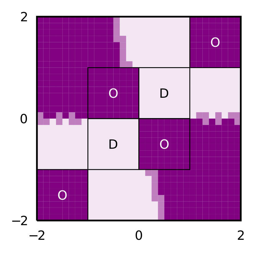
((a)) Known System

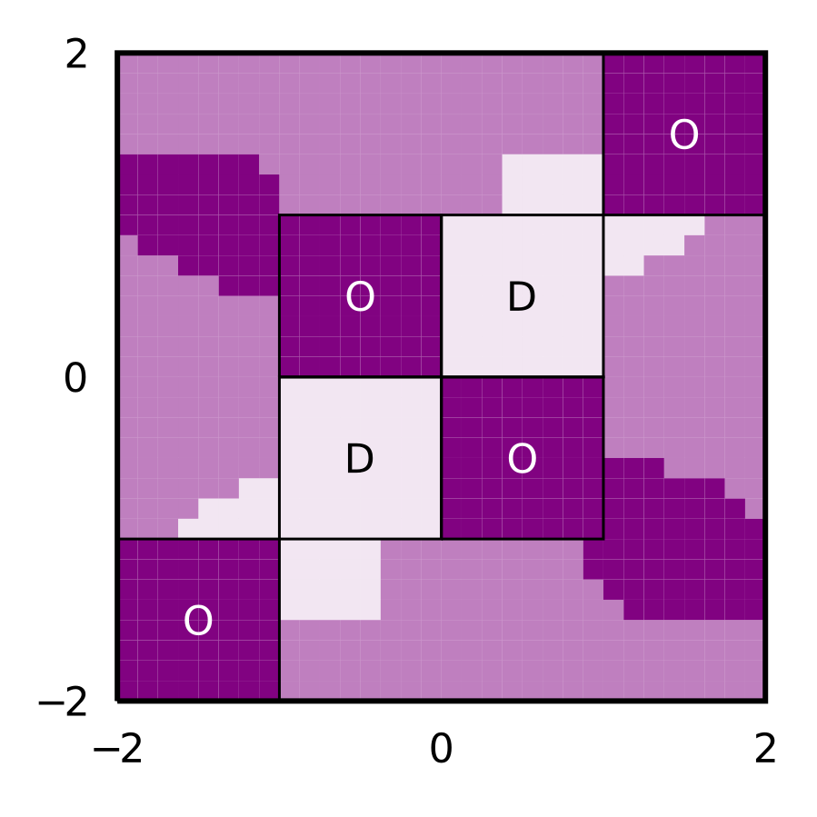
((b)) 100 data points

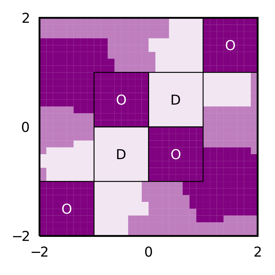
((c)) 500 data points

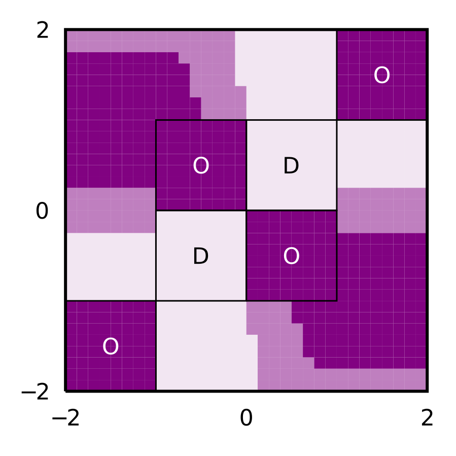
((d)) 2000 data points

Figure 2: The unbounded ($k=\infty$) verification results for the known system and learned system using increasingly large datasets subject to $\phi=\textnormal{P}_{\geq 0.95}[\neg O\leavevmode\nobreak\ \mathcal{U}\leavevmode\nobreak\ D$].

6.2 Parameter Considerations

The verification results on a linear system and computation times are compared for varying the learning error and discretization parameters, $\epsilon$ and $\Delta$ respectively, and the efficacy of using Proposition 4 to choose $\epsilon$ is highlighted. The unknown linear system is given by

$$\textnormal{{x}}(k+1=\begin{bmatrix}0.8&0.5\\ 0.0&0.5\end{bmatrix}\textnormal{{x}}(k),\quad\textnormal{{y}}(k)=\textnormal{{x}}(k)+\mathbf{v}(k).$$

The specification is the safety formula $\textnormal{P}_{\geq 0.95}[\mathcal{G}\leavevmode\nobreak\ X]$, i.e., the lower-bound of the probability of remaining within $X$ is at least 95%.

We used 200 datapoints for the verification of this system. To compare the effect of $\epsilon$, we manually selected values to be applied for every transition and compared the results with using the criterion in Proposition 4. The discretization fineness is studied by varying $\Delta$ to produce abstractions consisting of 37 states up to 1601 states. Figure 3 compares the average satisfaction probability interval sizes defined by

$$\bar{p}=\frac{1}{|Q|}\sum_{q\in Q}\hat{p}(q)-\check{p}(q)$$

where a smaller value indicates more certain intervals i.e., upper bound and lower bound probabilities are similar. As the uniform choice of $\epsilon$ approaches 0.45, the average probability interval size decreases although this trend reverses as $\epsilon$ decreases further. This is due to $\epsilon$ becoming too small to get non-zero regression error probabilities from Proposition 1. However, by applying Proposition 4, we obtain an optimal value for $\epsilon$ for every region pair, resulting in the smallest interval averages $\bar{p}$ for every discretization.

Note that there is an asymptotic decay in the average probability interval size, using a finer discretization. This however comes at a higher computation cost. The total computation times for framework components are shown in Table 1. The first and most demanding step involves discretizing $X$ and determining the image over-approximation and error upper bound of each state as discussed in Section 4.2. As implemented, this step takes 3-4 seconds per discrete state and is parallelized across 16 threads. The transition probability interval calculations involve checking the intersections between the image over-approximations and their respective target states. The unbounded verification procedure is fast relative to the time it takes to construct the IMDP abstraction using the previous two steps.

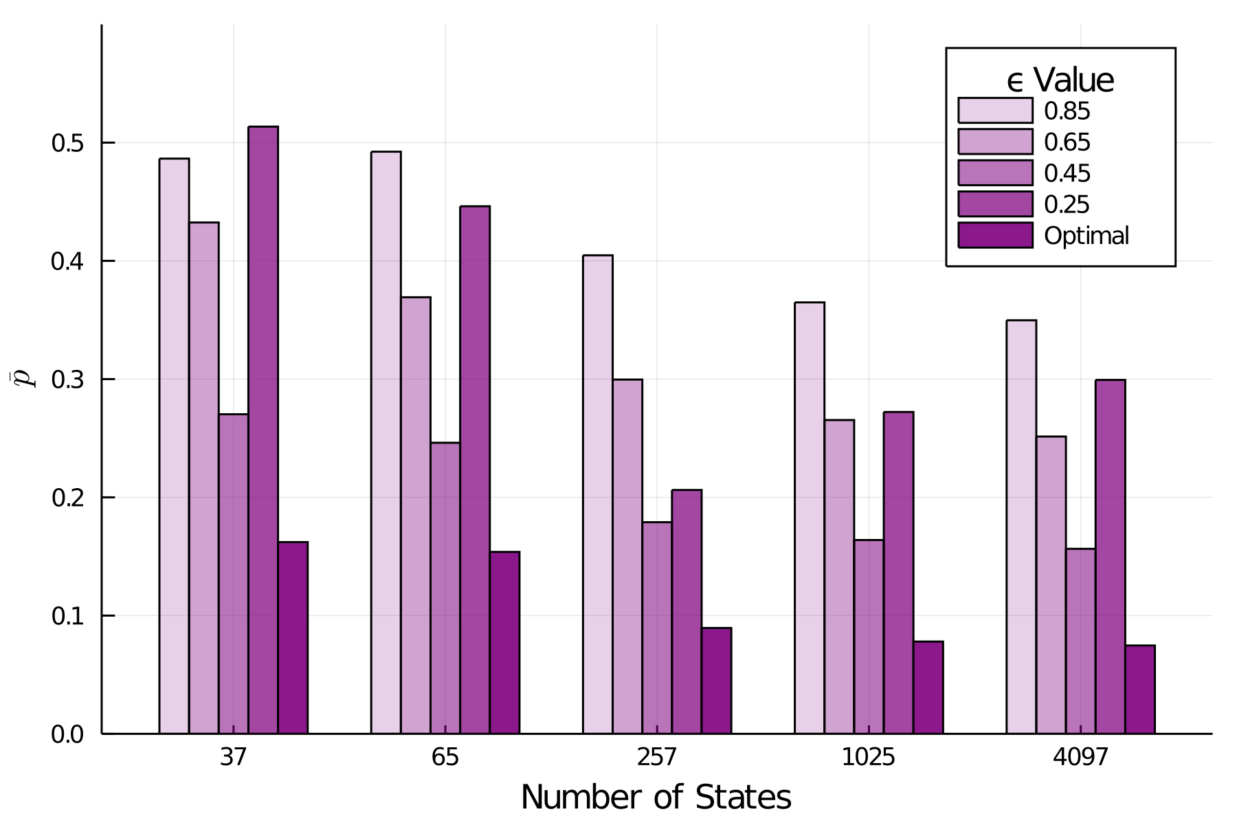
Figure 3: Effect of the size of discretization and $\epsilon$ on the average satisfaction probability interval size (verification error).

Table 1: Component computation times for an increasing number of states. Components include discretization and image over-approximations, transition probability interval calculations, and final verification times in seconds.

States	Computation Time (s)
	Disc. + Images	Transitions	Verification
65	$15.9$	$0.0476$	$0.0043$
122	$33.9$	$0.137$	$0.0070$
257	$62.4$	$0.613$	$0.0183$
485	$168$	$2.03$	$0.0370$
1025	$347$	$8.68$	$0.105$
1601	$482$	$20.0$	$0.225$

6.3 Switched System

We extend the previous example to demonstrate the verification of a system with multiple actions. The unknown system has two actions $A=\{a_{1},a_{2}\}$ where actions indicate

$$f(\textnormal{{x}}(k),a_{1})=\begin{bmatrix}0.8&0.5\\ 0.0&0.5\end{bmatrix},\quad f(\textnormal{{x}}(k),a_{2})=\begin{bmatrix}0.5&0\\ -0.5&0.8\end{bmatrix}.$$

Verification was performed subject to $\phi=\textnormal{P}_{\geq 0.95}[\mathcal{G}^{\leq k}\leavevmode\nobreak\ X]$ (paths of length $k$ should remain in $X$ with probability at least 95%) using $400$ datapoints for each action to construct the GPs. The $k=1$ and $k=\infty$ results, in Figures 4(a) and 4(b) respectively, show the regions where the system satisfies $\phi$ regardless of which action is selected. The framework can handle a system with an arbitrary number actions so long there is data available for each action.

((a)) $k=1$

((b)) $k=\infty$

Figure 4: Verification results for the switched system subject to $\phi=\textnormal{P}_{\geq 0.95}[\mathcal{G}^{\leq k}\leavevmode\nobreak\ Safe]$.

6.4 Nonlinear System

Finally, we perform verification on the nonlinear system given by

$$f(\textnormal{{x}}(k))=\textnormal{{x}}(k)+0.2\begin{bmatrix}\textnormal{{x}}^{(2)}(k)+(\textnormal{{x}}^{(2)}(k))^{2}e^{\textnormal{{x}}^{(1)}(k)}\\ \textnormal{{x}}^{(1)}(k)\end{bmatrix}$$

with the vector field shown in Figure 5(a). The system is unstable about its equilibrium points at $(0,0)$ and $(0,-1)$ and slows as it approaches them. The flow enters the set $X$ in the upper-left quadrant, and exits in the others. This nonlinear system could represent a closed-loop controller with dangerous operating conditions near the equilibria that should be avoided.

A 2000-point dataset is used for GP regression with the learned vector fields shown in Figure 5(b). The specification $\phi=\textnormal{P}_{\geq 0.95}[\neg O\leavevmode\nobreak\ \mathcal{U}^{\leq k}D]$ commands to avoid $O$ and remain within $X$ until $D$ is reached within $k$ steps. With $\Delta=0.03125$, the uniform discretization yields 16,384 discrete states which culminated into an end-to-end verification runtime of 91.2 hours. The majority of this time involved computing the images and error bounds for each discrete state, which is the only parallelized part of the framework.

For $k=1$ shown in Figure 5(c), $Q^{\text{yes}}$ consists of the $D$ regions and nearby states that transition to the $D$ regions with high probability. The size of the $Q^{\text{?}}$ buffer between $Q^{\text{yes}}$ and $Q^{\text{no}}$ provides a qualitative measure of the uncertainty embedded in the abstraction. As $k$ increases, $Q^{\text{yes}}$ modestly grows while $Q^{\text{no}}$ shrinks. The $k=\infty$ result shown in Figure 5(f) indicates where guarantees of satisfying or violating $\phi$ can be made over an unbounded horizon. There are many more states in $Q^{\text{yes}}$ as compared to even the $k=3$ result. The increase of $Q^{\text{?}}$ from $k=1$ to $k=\infty$ is due to the propagating learning and discretization uncertainty over longer horizons. The discretization resolution plays an important role in the size of $Q^{\text{?}}$, as the uncertain regions are easily induced by discrete states with possible self-transitions, which is mitigated with finer discretizations.

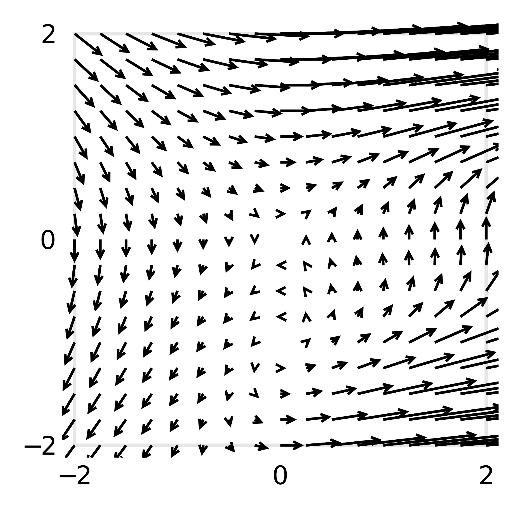
((a)) True vector field

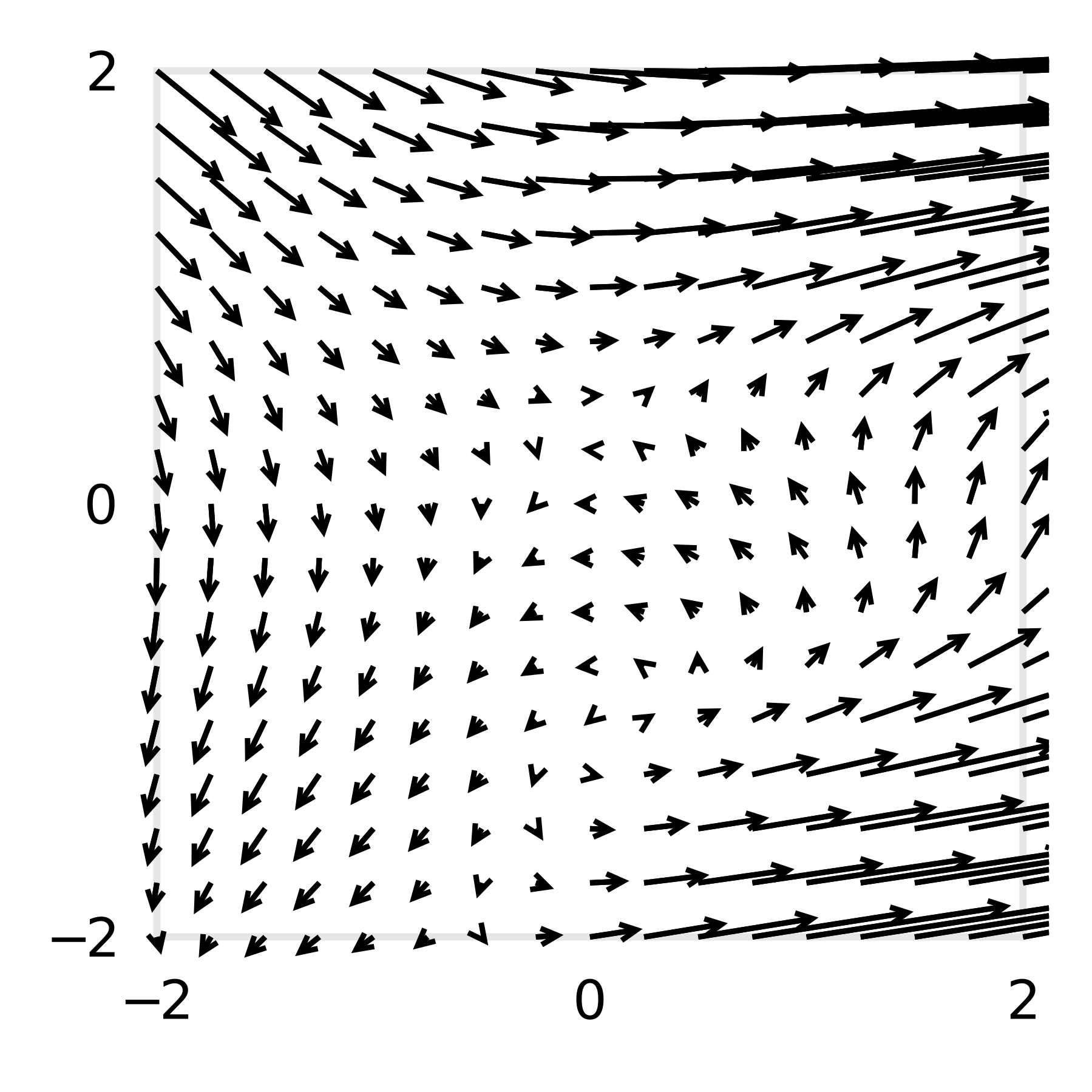
((b)) Learned vector field

((c)) $k=1$

((d)) $k=2$

((e)) $k=3$

((f)) $k=\infty$

Figure 5: Verification results for the nonlinear system subject to $\phi=\textnormal{P}_{\geq 0.95}[O\leavevmode\nobreak\ \mathcal{U}^{\leq k}D]$.

These case studies demonstrate the power of the end-to-end verification framework for abstract two-dimensional systems.

7 Final Remarks

We presented a verification framework for partially-observable, unknown dynamic systems subject to PCTL specifications. Through learning with Gaussian processes regression and sound interval Markov decision process abstraction of the system, we can achieve guarantees on satisfying (or violating) complex tasks even though the system dynamics are a priori unknown. Case studies for linear, switched and nonlinear systems illustrate its efficacy and highlight the opportunity for future applications in verifying the properties of complex autonomous systems.

These results can be used to find acceptable initial conditions (and avoid unacceptable ones) for system deployment, while highlighting regions for further uncertainty reduction through active learning or discretization refinement. Extensions to the framework could address partial state-observability for synthesis, and the scaling issues of GP regression and the over-approximations of state images and posterior covariance suprema. Our approach for partially-observable systems depends on the knowledge of the initial state in the dataset, which is a limitation for real-world applicability. While effective for GP regression, our interval-based abstraction method may be applied to other types of learning-based approaches provided sound probabilistic errors are available.

Declaration of Competing Interest

The authors declare that they have no known competing financial interests or personal relationships that could have appeared to influence the work reported in this paper.

Appendix A Proof of Proposition 2

Proof.

The proof relies on the following lemma, which gives equivalent conditions involving a function $f$ in an RKHS $\mathcal{H}$, its RKHS norm $\|f\|_{\kappa}$, and the associated kernel $\kappa$.

Lemma 2 (Theorem 3.11 from [40]).

Let $\mathcal{H}$ be an RKHS on $X$ with reproducing kernel $\kappa$ and let $\mathrm{f}\mathrel{\mathop{\mathchar 58\relax}}X\to\mathbb{R}$ be a function. Then the following are equivalent:

1. $\mathrm{f}\in\mathcal{H}$;

2. there exists a constant $c\geq 0$ such that, for every finite subset $F=\{x_{1},\dots x_{n}\}\subseteq X$, there exists a function $h\in\mathcal{H}$ with $\|h\|_{\kappa}\leq c$ and $\mathrm{f}(x_{i})=h(x_{i})$ for all $i=1,\dots n$;

3. there exists a constant $c\geq 0$ such that the function $c^{2}\kappa(x,x^{\prime})-\mathrm{f}(x)\mathrm{f}(x^{\prime})$ is a kernel function.

Moreover, if $\mathrm{f}\in\mathcal{H}$ then $\|\mathrm{f}\|_{\kappa}$ is the least $c$ that satisfies the inequalities in (ii) and (iii).

Let $\mathrm{f}\mathrel{\mathop{\mathchar 58\relax}}X\to\mathbb{R}$ reside in the RKHS $\mathcal{H}$ defined by $\kappa$. Note that any $c$ that satisfies (iii) in Lemma 2 also satisfies (ii). due to the assumption that $\mathrm{f}\in\mathcal{H}$ and choosing $h=\mathrm{f}$.

A kernel function $\kappa$ is positive semidefinite if and only if, for all finite subsets $\{x_{1},\dots x_{n}\}\subset X$ and real vectors $\{b_{1},\dots b_{n}\}\in\mathbb{R}^{n}$, $\sum_{i}\sum_{j}\kappa(x_{i},x_{j})b_{i}b_{j}\geq 0$ which the given kernel satisfies. By Lemma 2, there exists a constant $c\geq 0$ such that

$$\sum_{i}\sum_{j}(c^{2}\kappa(x_{i},x_{j})-\mathrm{f}(x_{i})\mathrm{f}(x_{j}))b_{i}b_{j}$$

$$= \sum_{i}\sum_{j}\kappa(x_{i},x_{j})b_{i}b_{j}-c^{-2}\mathrm{f}(x_{i})\mathrm{f}(x_{j})b_{i}b_{j}$$

$$= \sum_{i}\sum_{j}\kappa(x_{i},x_{j})b_{i}b_{j}-\sum_{i}\sum_{j}c^{-2}\mathrm{f}(x_{i})\mathrm{f}(x_{j})b_{i}b_{j}\geq 0$$

which leads to

$$\sum_{i}\sum_{j}\kappa(x_{i},x_{j})b_{i}b_{j}\geq\sum_{i}\sum_{j}c^{-2}\mathrm{f}(x_{i})\mathrm{f}(x_{j})b_{i}b_{j}$$

Assume $\kappa(x,x^{\prime})\geq 0$. The next step is to choose $c\geq 0$ such that, for all $i$ and $j$,

$$\kappa(x_{i},x_{j}) \geq|c^{-2}\mathrm{f}(x_{i})\mathrm{f}(x_{j})|$$

$$c^{2} \geq\frac{|\mathrm{f}(x_{i})\mathrm{f}(x_{j})|}{\kappa(x_{i},x_{j})}$$

which obligates the choice

$$c^{2} =\sup_{x,x^{\prime}\in X}\frac{|\mathrm{f}(x)\mathrm{f}(x^{\prime})|}{\kappa(x,x^{\prime})}$$ (13)

$$\leq\frac{\sup_{x\in X}f(x)^{2}}{\inf_{x,x^{\prime}\in X}\kappa(x,x^{\prime})}.$$ (14)

By Lemma 2, the right-hand side expression in 14 is an upper bound of $\|\mathrm{f}\|^{2}_{\kappa}$. ∎

Appendix B Proof of Proposition 3

Proof.

The proof relies on Hadamard’s determinant bounding inequality and $s=\sup_{x\in X}\kappa(x,x)$. For any kernel matrix $K$, the information gain term is bounded by

$$\log|I+\sigma^{-2}K| \leq\log\prod_{i=1}^{d}|1+\sigma^{-2}K_{i,i})|$$

$$\leq\log\prod_{i=1}^{d}|1+\sigma^{-2}s|$$

$$=\sum_{i=1}^{d}\log(1+\sigma^{-2}s)$$

$$=d\log(1+\sigma^{-2}s).$$

∎

Appendix C Proof of Proposition 4

Proof.

Let $\textnormal{P}(\epsilon_{i})=(1-\delta_{i}(\epsilon_{i}))$ denote the CDF of the probabilistic regression error. In order to maximize the upper bound in Theorem 1, the indicator function should return 1 and the product with $\textnormal{P}(\epsilon_{i})$ should be maximizing. The indicator function returns 1 if $Im(q,a)\cap\underline{q^{\prime}}=Im(q,a)$. The most $q^{\prime}$ can shrink is

$$\inf_{a\in\partial Im(q,a),b\in\partial q^{\prime}}|a-b|.$$

Since $\textnormal{P}(\epsilon_{i})$ is non-decreasing, the choice of $\epsilon$ is maximizing. The proof for the minimizing case is similar. ∎

Appendix D Proof of Lemma 1

Proof.

Assume, for simplicity and without any loss of generality, that $\pi_{\mathbf{y}}$ is stationary. Then $V_{k}^{\pi_{\mathbf{y}}}\mathrel{\mathop{\mathchar 58\relax}}\mathbb{R}^{n}\to\mathbb{R}$ is defined recursively as

$$V_{k}^{\pi_{\mathbf{y}}}(x)=\begin{cases}1&\text{if }x\in X^{1}\\ 0&\text{if }x\in X^{0}\\ 0&\text{if }x\notin(X^{0}\cup X^{1})\wedge k=0\\ \mathbf{E}_{v\sim p_{\mathbf{v}},\,\bar{x}\sim T(\cdot\mid x,\pi_{\mathbf{y}}(x+v))}[V_{k-1}(\bar{x})]&\text{otherwise.}\end{cases}$$

To prove Lemma 1, we need to show that

$$V_{k}^{\pi_{\mathbf{y}}}(x)=\textnormal{P}(\omega^{k}_{\textnormal{{x}}}\models\psi\mid\omega_{\textnormal{{x}}}(0)=x,\pi_{\mathbf{y}}),$$

that is the probability that a path of length $k$ of Process (1) initialized at $x$ is equal to $V_{k}^{\pi_{\mathbf{y}}}(x).$

The proof is by induction over the length of the path. The base case is

$$\textnormal{P}(\omega^{0}_{\textnormal{{x}}}\models\psi\mid\omega^{0}_{\textnormal{{x}}}(0)=x,\pi_{\mathbf{y}})=\mathbf{1}_{X^{1}}(x)=V_{0}^{\pi_{\mathbf{y}}}(x).$$

Then, to conclude the proof we need to show that under the assumption that for all $x\in\mathbb{R}^{n}$

$$\textnormal{P}(\omega^{k-1}_{\textnormal{{x}}}\models\psi\mid\omega_{\textnormal{{x}}}(0)=x)=V_{k-1}^{\pi_{\mathbf{y}}}(x),$$

it holds that for all $x\in\mathbb{R}^{n}$

$$\textnormal{P}(\omega^{k}_{\textnormal{{x}}}\models\psi\mid\omega_{\textnormal{{x}}}(0)=x,\pi_{\mathbf{y}})=V_{k}^{\pi_{\mathbf{y}}}(x).$$

Call $\bar{X}=X\setminus(X^{0}\cup X^{1}),$ that is the complement of set $X^{0}\cup X^{1}$, and define notation

$$\omega^{k}_{\textnormal{{x}}}([i,k-1])\in X\mathrel{\mathop{\mathchar 58\relax}}=\forall j\in[i,k-1],\,\omega^{k}_{\textnormal{{x}}}(j)\in X.$$

Assume without loss of generality that $x\in\bar{X},$ then the remaining part of the proof is as follows:

$$\textnormal{P}(\omega^{k}_{\textnormal{{x}}}\models\psi\mid\omega_{\textnormal{{x}}}(0)=x,\pi_{\mathbf{y}})$$

$$=\sum_{i=1}^{k}\textnormal{P}(\omega^{k}_{\textnormal{{x}}}(i)\in X^{1}\wedge\omega^{k}_{\textnormal{{x}}}([1,i-1])\in\bar{X}\mid\omega^{k}_{\textnormal{{x}}}(0)=x,\pi_{\mathbf{y}})$$

$$=\textnormal{P}(\omega^{k}_{\textnormal{{x}}}(1)\in X^{1}\mid\omega^{k}_{\textnormal{{x}}}(0)=x,\pi_{\mathbf{y}})\,+$$

$$\hskip 36.98866pt\sum_{i=2}^{k}\textnormal{P}(\omega^{k}_{\textnormal{{x}}}(i)\in X^{1}\wedge\omega^{k}_{\textnormal{{x}}}([1,i-1])\in\bar{X}\mid\omega^{k}_{\textnormal{{x}}}(0)=x,\pi_{\mathbf{y}})$$

$$=\int\int_{X^{1}}t(\bar{x}\mid x,\pi_{\mathbf{y}}(x+v))p_{\mathbf{v}}(v)d\bar{x}dv\,+$$

$$\quad\sum_{i=2}^{k}\int\int_{\bar{X}}\textnormal{P}(\omega^{k}_{\textnormal{{x}}}(i)\in X^{1}\wedge\omega^{k}_{\textnormal{{x}}}([2,i-1])\in\bar{X}\mid\omega^{k}_{\textnormal{{x}}}(1)=\bar{x},\pi_{\mathbf{y}})$$

$$\hskip 139.41832ptt(\bar{x}\mid x,\pi_{\mathbf{y}}(x+v))p_{\mathbf{v}}(v)d\bar{x}dv$$

$$=\int\int_{X^{1}}t(\bar{x}\mid x,\pi_{\mathbf{y}}(x+v))p_{\mathbf{v}}(v)d\bar{x}dv\,+$$

$$\quad\sum_{i=1}^{k-1}\int\int_{\bar{X}}\textnormal{P}\big{(}\omega^{k-1}_{\textnormal{{x}}}(i)\in X^{1}\wedge\omega^{k-1}_{\textnormal{{x}}}([1,i-1])\in\bar{X}\mid$$

$$\hskip 76.82234pt\omega^{k-1}_{\textnormal{{x}}}(0)=\bar{x},\pi_{\mathbf{y}}\big{)}\,t(\bar{x}\mid x,\pi_{\mathbf{y}}(x+v))p_{\mathbf{v}}(v)d\bar{x}dv$$

$$=\int\int\big{(}\mathbf{1}_{X^{1}}(\bar{x})+\mathbf{1}_{\bar{X}}(\bar{x})\,\textnormal{P}(\omega^{k-1}_{\textnormal{{x}}}\models\psi\mid\omega_{\textnormal{{x}}}(0)=\bar{x},\pi_{\mathbf{y}})\big{)}$$

$$\hskip 139.41832ptt(\bar{x}\mid x,\pi_{\mathbf{y}}(x+v))p_{\mathbf{v}}(v)d\bar{x}dv$$

$$=\int\int\textnormal{P}(\omega^{k-1}_{\textnormal{{x}}}\models\psi\mid\omega_{\textnormal{{x}}}(0)=\bar{x},\pi_{\mathbf{y}})t(\bar{x}\mid x,\pi_{\mathbf{y}}(x+v))p_{\mathbf{v}}(v)d\bar{x}dv$$

$$=V_{k}^{\pi_{\mathbf{y}}}(x),$$

where in the third equality we marginalized over the event $\omega^{k}_{\textnormal{{x}}}(1)=\bar{x}$ and use the definition of conditional probability, and in the fourth equality we use that for $i<k$ and $x\in\bar{X}$

$$\textnormal{P}(\omega^{k-1}_{\textnormal{{x}}}(i)\in X^{1}\wedge\omega^{k-1}_{\textnormal{{x}}}([1,i-1])\in\bar{X}\mid\omega^{k-1}_{\textnormal{{x}}}(0)=\bar{x},\pi_{\mathbf{y}})=\\ \textnormal{P}(\omega^{k}_{\textnormal{{x}}}(i+1)\in X^{1}\wedge\omega^{k}_{\textnormal{{x}}}([2,i+1-1])\in\bar{X}\mid\omega^{k}_{\textnormal{{x}}}(1)=\bar{x},\pi_{\mathbf{y}}),$$

which holds because of the Markov property.

∎

References

- [1] Alessandro Abate, Frank Redig, and Ilya Tkachev. On the effect of perturbation of conditional probabilities in total variation. Statistics & Probability Letters, 88:1–8, 2014.
- [2] Mohamadreza Ahmadi, Arie Israel, and Ufuk Topcu. Safety assessemt based on physically-viable data-driven models. In 2017 IEEE 56th Annual Conference on Decision and Control (CDC), pages 6409–6414. IEEE, 2017.
- [3] Anayo K Akametalu, Shahab Kaynama, Jaime F Fisac, Melanie N Zeilinger, Jeremy H Gillula, and Claire J Tomlin. Reachability-based safe learning with Gaussian processes. In IEEE 53rd Annual Conference on Decision and Control (CDC), 2014: 15-17 Dec. 2014, Los Angeles, California, USA, pages 1424–1431. IEEE, 2014.
- [4] Christel Baier and Joost-Pieter Katoen. Principles of Model Checking. The MIT Press, Cambridge, MA, 2008.
- [5] Christel Baier, Joost-Pieter Katoen, et al. Principles of model checking, volume 26202649. MIT press Cambridge, 2008.
- [6] Christel Baier, Joost-Pieter Katoen, and Kim Guldstrand Larsen. Principles of model checking. 2008.
- [7] Calin Belta, Boyan Yordanov, and Ebru Aydin Gol. Formal methods for discrete-time dynamical systems, volume 89. Springer, 2017.
- [8] Felix Berkenkamp, Riccardo Moriconi, Angela P Schoellig, and Andreas Krause. Safe learning of regions of attraction for uncertain, nonlinear systems with gaussian processes. In 2016 IEEE 55th Conference on Decision and Control (CDC), pages 4661–4666. IEEE, 2016.
- [9] Felix Berkenkamp, Matteo Turchetta, Angela Schoellig, and Andreas Krause. Safe model-based reinforcement learning with stability guarantees. In Advances in neural information processing systems, pages 908–918, 2017.
- [10] Dimitir P Bertsekas and Steven Shreve. Stochastic optimal control: the discrete-time case. 2004.
- [11] Arno Blaas, Andrea Patane, Luca Laurenti, Luca Cardelli, Marta Kwiatkowska, and Stephen Roberts. Adversarial robustness guarantees for classification with gaussian processes. In International Conference on Artificial Intelligence and Statistics, pages 3372–3382. PMLR, 2020.
- [12] Cristóbal Camarero. Simple, fast and practicable algorithms for cholesky, lu and qr decomposition using fast rectangular matrix multiplication. arXiv preprint arXiv:1812.02056, 2018.
- [13] Nathalie Cauchi, Luca Laurenti, Morteza Lahijanian, Alessandro Abate, Marta Kwiatkowska, and Luca Cardelli. Efficiency through uncertainty: Scalable formal synthesis for stochastic hybrid systems. In Proceedings of the 22nd ACM International Conference on Hybrid Systems: Computation and Control, pages 240–251, 2019.
- [14] Sayak Ray Chowdhury and Aditya Gopalan. On kernelized multi-armed bandits. In Proceedings of the 34th International Conference on Machine Learning-Volume 70, pages 844–853. JMLR. org, 2017.
- [15] E. M. Clarke, O. Grumberg, and D. Peled. Model Checking. MIT Press, 1999.
- [16] Giannis Delimpaltadakis, Luca Laurenti, and Manuel Mazo Jr. Abstracting the sampling behaviour of stochastic linear periodic event-triggered control systems. CDC, 2021.
- [17] Laurent Doyen, Goran Frehse, George J Pappas, and André Platzer. Verification of hybrid systems. In Handbook of Model Checking, pages 1047–1110. Springer, 2018.
- [18] Antoine Girard and George J. Pappas. Approximation metrics for discrete and continuous systems. IEEE Transactions on Automatic Control, 52(5):782–798, 2007.
- [19] Robert Givan, Sonia Leach, and Thomas Dean. Bounded-parameter Markov decision processes. Artificial Intelligence, 122(1-2):71–109, 2000.
- [20] Sofie Haesaert, Paul MJ Van den Hof, and Alessandro Abate. Data-driven and model-based verification via bayesian identification and reachability analysis. Automatica, 79:115–126, 2017.
- [21] Ernst Moritz Hahn, Vahid Hashemi, Holger Hermanns, Morteza Lahijanian, and Andrea Turrini. Multi-objective robust strategy synthesis for interval Markov decision processes. In Int. Conf. on Quantitative Evaluation of SysTems (QEST), pages 207–223, Berlin, Germany, Sep. 2017. Springer.
- [22] Ernst Moritz Hahn, Vahid Hashemi, Holger Hermanns, Morteza Lahijanian, and Andrea Turrini. Interval Markov decision processes with multiple objectives: From robust strategies to pareto curves. ACM Transactions on Modeling and Computer Simulation, 29(4):1–31, 2019.
- [23] Mohamed K Helwa, Adam Heins, and Angela P Schoellig. Provably Robust Learning-Based Approach for High-Accuracy Tracking Control of Lagrangian Systems. IEEE Robotics and Automation Letters, 4(2):1587–1594, 2019.
- [24] Eyke Hüllermeier and Willem Waegeman. Aleatoric and epistemic uncertainty in machine learning: An introduction to concepts and methods. Machine Learning, 110(3):457–506, 2021.
- [25] Radoslav Ivanov, Taylor J. Carpenter, James Weimer, Rajeev Alur, George J. Pappas, and Insup Lee. Verifying the Safety of Autonomous Systems with Neural Network Controllers. ACM Transactions on Embedded Computing Systems (TECS), 20(1):1–26, 2020.
- [26] John Jackson, Luca Laurenti, Eric Frew, and Morteza Lahijanian. Safety verification of unknown dynamical systems via gaussian process regression. In 2020 59th IEEE Conference on Decision and Control (CDC), pages 860–866. IEEE, 2020.
- [27] John Jackson, Luca Laurenti, Eric Frew, and Morteza Lahijanian. Strategy synthesis for partially-known switched stochastic systems. In Proceedings of the 24th International Conference on Hybrid Systems: Computation and Control, HSCC ’21, New York, NY, USA, 2021. Association for Computing Machinery.
- [28] P. Jagtap, G. J. Pappas, and M. Zamani. Control barrier functions for unknown nonlinear systems using gaussian processes*. In 2020 59th IEEE Conference on Decision and Control (CDC), pages 3699–3704, 2020.
- [29] Joris Kenanian, Ayca Balkan, Raphael M Jungers, and Paulo Tabuada. Data driven stability analysis of black-box switched linear systems. Automatica, 109:108533, 2019.
- [30] Harold Kushner and Paul G Dupuis. Numerical methods for stochastic control problems in continuous time, volume 24. Springer Science & Business Media, 2013.
- [31] Morteza Lahijanian, Sean B. Andersson, and Calin Belta. Approximate markovian abstractions for linear stochastic systems. In Proc. of the IEEE Conference on Decision and Control, Dec 2012. (submitted).
- [32] Morteza Lahijanian, Sean B. Andersson, and Calin Belta. Formal verification and synthesis for discrete-time stochastic systems. IEEE Transactions on Automatic Control, 60(8):2031–2045, Aug. 2015.
- [33] Luca Laurenti, Morteza Lahijanian, Alessandro Abate, Luca Cardelli, and Marta Kwiatkowska. Formal and efficient synthesis for continuous-time linear stochastic hybrid processes. IEEE Transactions on Automatic Control, 2020.
- [34] Armin Lederer, Jonas Umlauft, and Sandra Hirche. Uniform error bounds for gaussian process regression with application to safe control. In Advances in Neural Information Processing Systems, pages 657–667, 2019.
- [35] Ryan Luna, Morteza Lahijanian, Mark Moll, and Lydia E. Kavraki. Asymptotically optimal stochastic motion planning with temporal goals. In The Eleventh International Workshop on the Algorithmic Foundations of Robotics (WAFR), pages 335–352, Istanbul, Turkey, Aug. 2014.
- [36] Ryan Luna, Morteza Lahijanian, Mark Moll, and Lydia E. Kavraki. Fast stochastic motion planning with optimality guarantees using local policy reconfiguration. In IEEE Conference on Robotics and Automation, pages 3013–3019, Hong Kong, China, May 2014.
- [37] Ryan Luna, Morteza Lahijanian, Mark Moll, and Lydia E. Kavraki. Optimal and efficient stochastic motion planning in partially-known environments. In The Twenty-Eighth AAAI Conference on Artificial Intelligence, pages 2549–2555, Quebec City, Canada, July 2014. AAAI Press.
- [38] Pascal Massart. Concentration inequalities and model selection, volume 6. Springer, 2007.
- [39] Charles A Micchelli, Yuesheng Xu, and Haizhang Zhang. Universal Kernels. Journal of Machine Learning Research, 7, 2006.
- [40] Vern I Paulsen and Mrinal Raghupathi. An introduction to the theory of reproducing kernel Hilbert spaces, volume 152. Cambridge University Press, 2016.
- [41] Gilles Perrouin, Mathieu Acher, Maxime Cordy, Xavier Devroey, Hojat Khosrowjerdi, and Karl Meinke. Learning-based testing for autonomous systems using spatial and temporal requirements. Proceedings of the 1st International Workshop on Machine Learning and Software Engineering in Symbiosis, pages 6–15, 2018.
- [42] Carl Edward Rasmussen. Gaussian processes in machine learning. In Summer School on Machine Learning, pages 63–71. Springer, 2003.
- [43] Sadegh Esmaeil Zadeh Soudjani, Caspar Gevaerts, and Alessandro Abate. Faust2: Formal abstractions of uncountable-state stochastic processes. In International Conference on Tools and Algorithms for the Construction and Analysis of Systems, pages 272–286. Springer, 2015.
- [44] Alireza Souri, Amin Salih Mohammed, Moayad Yousif Potrus, Mazhar Hussain Malik, Fatemeh Safara, and Mehdi Hosseinzadeh. Formal Verification of a Hybrid Machine Learning-Based Fault Prediction Model in Internet of Things Applications. IEEE Access, 8:23863–23874, 2020.
- [45] Niranjan Srinivas, Andreas Krause, Sham M Kakade, and Matthias W Seeger. Information-theoretic regret bounds for gaussian process optimization in the bandit setting. IEEE Transactions on Information Theory, 58(5):3250–3265, 2012.
- [46] Ingo Steinwart. On the influence of the kernel on the consistency of support vector machines. Journal of machine learning research, 2(Nov):67–93, 2001.
- [47] Yanan Sui, Alkis Gotovos, Joel W Burdick, and Andreas Krause. Safe exploration for optimization with gaussian processes. Proceedings of Machine Learning Research, 37:997–1005, 2015.
- [48] Paulo Tabuada. Verification and control of hybrid systems: a symbolic approach. Springer Science & Business Media, 2009.
- [49] Sattar Vakili, Kia Khezeli, and Victor Picheny. On Information Gain and Regret Bounds in Gaussian Process Bandits. arXiv, 2020.
- [50] Zheming Wang and Raphaël M. Jungers. Scenario-Based Set Invariance Verification for Black-Box Nonlinear Systems. IEEE Control Systems Letters, 5(1):193–198, 2021.
- [51] M Wicker, A Patane, A Abate, L Laurenti, M Kwiatkowska, et al. Certification of iterative predictions in bayesian neural networks. In Proceedings of the Conference on Uncertainty in Artificial Intelligence. PMLR, 2021.
- [52] Weiming Xiang, Patrick Musau, Ayana A. Wild, Diego Manzanas Lopez, Nathaniel Hamilton, Xiaodong Yang, Joel Rosenfeld, and Taylor T. Johnson. Verification for machine learning, autonomy, and neural networks survey, 2018.
- [53] Hansol Yoon, Yi Chou, Xin Chen, Eric Frew, and Sriram Sankaranarayanan. Predictive runtime monitoring for linear stochastic systems and applications to geofence enforcement for uavs. In International Conference on Runtime Verification, pages 349–367. Springer, 2019.