Energy Landscape of State-Specific Electronic Structure Theory

Abstract

State-specific approximations can provide an accurate representation of challenging electronic excitations by enabling relaxation of the electron density. While state-specific wave functions are known to be local minima or saddle points of the approximate energy, the global structure of the exact electronic energy remains largely unexplored. In this contribution, a geometric perspective on the exact electronic energy landscape is introduced. On the exact energy landscape, ground and excited states form stationary points constrained to the surface of a hypersphere and the corresponding Hessian index increases at each excitation level. The connectivity between exact stationary points is investigated and the square-magnitude of the exact energy gradient is shown to be directly proportional to the Hamiltonian variance. The minimal basis Hartree–Fock and Excited-State Mean-Field representations of singlet H2 (STO-3G) are then used to explore how the exact energy landscape controls the existence and properties of state-specific approximations. In particular, approximate excited states correspond to constrained stationary points on the exact energy landscape and their Hessian index also increases for higher energies. Finally, the properties of the exact energy are used to derive the structure of the variance optimisation landscape and elucidate the challenges faced by variance optimisation algorithms, including the presence of unphysical saddle points or maxima of the variance.

I Introduction

Including wave function relaxation in state-specific approximations can provide an accurate representation of excited states where there is significant electron density rearrangement relative to the electronic ground state. This relaxation is particularly important for the description of charge transfer,Barca et al. (2018); Liu et al. (2012); Jensen et al. (2018); Shea and Neuscamman (2018); Hait and Head-Gordon (2021) core electron excitations,Hait and Head-Gordon (2020); Oosterbaan et al. (2018, 2020); Garner and Neuscamman (2020) or Rydberg states with diffuse orbitals,Carter-Fenk and Herbert (2020); Shea and Neuscamman (2018); Clune et al. (2020) and can be visualised using the eigenvectors of the difference density matrix for the excitation.Plasser et al. (2014, 2014) In contrast, techniques based on linear response theory — including time-dependent Hartree–FockMcLachlan and Ball (1964) (TD-HF), time-dependent density functional theoryRunge and Gross (1984); Dreuw and Head-Gordon (2005); Burke et al. (2005) (TD-DFT), configuration interaction singlesForesman et al. (1992); Dreuw and Head-Gordon (2005) (CIS), and equation of motion coupled cluster theoryStanton and Bartlett (1993); Krylov (2008) (EOM-CC) — are evaluated using the ground-state orbitals, making a balanced treatment of the ground and excited states more difficult. Burke et al. (2005) Furthermore, linear response methods are generally applied under the adiabatic approximation and are limited to single excitations.Maitra et al. (2004); Burke et al. (2005) In principle, state-specific approaches can approximate both single and double excitations,Gilbert et al. (2008); Barca et al. (2018); Otis et al. (2020) although the open-shell character of single excitations requires a multi-configurational approach.Shea and Neuscamman (2018); Hardikar and Neuscamman (2020); Zhao and Neuscamman (2020, 2020); Ye et al. (2017)

Underpinning excited state-specific methods is the fundamental idea that ground-state wave functions can also be used to describe an electronic excited state. This philosophy relies on the existence of additional higher-energy mathematical solutions, which have been found in Hartree–Fock (HF),Slater (1951); Stanton (1968); Fukutome (1971, 1974, 1974, 1975, 1973); Mestechkin (1978, 1979, 1988); Davidson and Borden (1983); Kowalski and Jankowski (1998); Gilbert et al. (2008); Thom and Head-Gordon (2008); Li and Paldus (2009); Jiménez-Hoyos et al. (2011, 2014); Tóth and Pulay (2016); Burton et al. (2018); Huynh and Thom (2020); Lee and Head-Gordon (2019); Burton and Wales (2021) density functional theory (DFT),Theophilou (1979); Perdew and Levy (1985); Zarotiadis et al. (2020); Hait and Head-Gordon (2020) multiconfigurational self-consistent field (MC-SCF),Olsen et al. (1982); Golab et al. (1983); Olsen et al. (1983); Golab et al. (1985); Angeli et al. (2003); Guihery et al. (1997); Evenhuis and Martínez (2011); Tran et al. (2019); Tran and Neuscamman (2020) and coupled cluster (CC) theory.Piecuch and Kowalski (2000); Mayhall and Raghavachari (2010); Lee et al. (2019); Marie et al. (2021); Kossoski et al. (2021) These multiple solutions correspond to higher-energy stationary points of a parametrised approximate energy function, including local energy minima, saddle points, or maxima. It has long been known that the exact $k$-th excited state forms a saddle point of the energy with $k$ negative Hessian eigenvalues (where $k=0$ is the ground state). These stationary properties have been identified using the exponential parametrisation of MC-SCF calculationsWerner and Meyer (1981); Olsen et al. (1982); Golab et al. (1985); Olsen et al. (1983); Golab et al. (1983) and can also be derived using local expansions around an exact eigenstate.Bacalis et al. (2016); N. C. Bacalis (2020) However, questions remain about the global structure of the exact energy landscape and the connections between exact excited states.

Multiple self-consistent field (SCF) solutions in HF or Kohn–Sham DFT are the most widely understood state-specific approximations. Their existence was first identified by Slater,Slater (1951) and later characterised in detail by Fukutome.Fukutome (1971, 1974, 1974, 1975, 1973) Physically, these solutions appear to represent single-determinant approximations for excited states,Gilbert et al. (2008); Besley et al. (2009); Barca et al. (2014, 2018, 2018) or mean-field quasi-diabatic states.Thom and Head-Gordon (2009); Jensen et al. (2018) In the presence of strong electron correlation, multiple SCF solutions often break symmetries of the exact Hamiltonian Davidson and Borden (1983); Li and Paldus (2009); Huynh and Thom (2020); Jiménez-Hoyos et al. (2011, 2014); Lee and Head-Gordon (2019) and can disappear as the molecular geometry changes.Mestechkin (1978, 1979, 1988); Burton et al. (2018) The stability analysis pioneered by Čižek and PaldusČížek and Paldus (1967, 1970); Thouless (1960); Paldus and Čížek (1970) allows SCF solutions to be classified according to their Hessian index (the number of downhill orbital rotations). There are usually only a handful of low-energy SCF minima, connected by index-1 saddle points, while symmetry-broken solutions form several degenerate minima that are connected by higher-symmetry saddle points.Burton and Wales (2021) At higher energies, stationary points representing excited states generally become higher-index saddle points of the energy.Perdew and Levy (1985); Dardenne et al. (2000); Burton and Wales (2021)

Recent interest in locating higher-energy SCF solutions has led to several new approaches including: modifying the iterative SCF approach with orbital occupation constraintsGilbert et al. (2008); Barca et al. (2018) or level-shifting;Carter-Fenk and Herbert (2020) second-order direct optimisation of higher-energy stationary points;Levi et al. (2020, 2020) minimising an alternative functional such as the varianceYe et al. (2017); Ye and Van Voorhis (2019); Shea and Neuscamman (2017, 2018); Cuzzocrea et al. (2020) or the square-magnitude of the energy gradient.Hait and Head-Gordon (2020) The success of these algorithms depends on the structure of the approximate energy landscape, the stationary properties of excited states, and the quality of the initial guess. In principle, the approximate energy landscape is determined by the relationship between an approximate wave function and the exact energy landscape. However, the nature of this connection has not been widely investigated.

Beyond single-determinant methods, state-specific approximations using multi-configurational wave functions have been developed to describe open-shell or statically correlated excited states, including MC-SCF,Olsen et al. (1982); Golab et al. (1985); Olsen et al. (1983); Golab et al. (1983); Tran et al. (2019); Tran and Neuscamman (2020) excited-state mean-field (ESMF) theory,Shea and Neuscamman (2018); Hardikar and Neuscamman (2020); Zhao and Neuscamman (2020, 2020) half-projected HF,Ye and Van Voorhis (2019) or multi-Slater-Jastrow functions.Dash et al. (2019); Cuzzocrea et al. (2020); Dash et al. (2021) The additional complexity of these wave functions compared to a single determinant has led to the use of direct second-order optimisation algorithmsOlsen et al. (1982); Golab et al. (1985); Olsen et al. (1983); Golab et al. (1983); Werner and Meyer (1981) or, more recently, methods based on variance optimisation.Messmer (1969); Shea and Neuscamman (2017); Pineda Flores and Neuscamman (2019) Variance optimisation exploits the fact that both ground and excited states form minima of the Hamiltonian variance $\matrixelement*{\Psi}{(\mathcal{H}-E)^{2}}{\Psi}$,MacDonald (1934) and thus excited-states can be identified using downhill minimisation techniques. Alternatively, the folded-spectrum method uses an objective function with the form $\matrixelement*{\Psi}{(\mathcal{H}-\omega)^{2}}{\Psi}$ to target the state with energy closest to $\omega$.Wang and Zunger (1994) These approaches are particularly easy to combine with stochastic methods such as variational Monte–CarloUmrigar and Filippi (2005); Pineda Flores and Neuscamman (2019); Cuzzocrea et al. (2020) (VMC) and have been proposed as an excited-state extension of variational quantum eigensolvers.Zhang et al. (2020, 2021) However, variance optimisation is prone to convergence issues that include drifting away from the intended target state,Cuzzocrea et al. (2020); Otis et al. (2020) and very little is known about the properties of the variance optimisation landscape, or its stationary points.

In my opinion, our limited understanding about the relationship between exact and approximate state-specific solutions arises because exact electronic structure is traditionally viewed as a matrix eigenvalue problem, while state-specific approximations are considered as higher-energy stationary points of an energy landscape. The energy landscape concept is more familiar to theoretical chemists in the context of a molecular potential energy surface,Born and Oppenheimer (1927) where local minima correspond to stable atomic arrangements and index-1 saddles can be interpreted as reactive transition states.Murrell and Laidler (1968); Wales (2004) To bridge these concepts, this article introduces a fully geometric perspective on exact electronic structure within a finite Hilbert space. In this representation, ground and excited states form stationary points of an energy landscape constrained to the surface of a unit hypersphere. Analysing the differential geometry of this landscape reveals the stationary properties of ground and excited states and the pathways that connect them. Furthermore, the square-magnitude of the exact gradient is shown to be directly proportional to the Hamiltonian variance, allowing the structure of the exact variance optimisation landscape to be derived. Finally, the relationship between approximate wave functions and the exact energy or variance is explored, revealing how the stationary properties of state-specific solutions are controlled by the structure of the exact energy landscape.

Throughout this work, key concepts are illustrated using the electronic singlet states of H2. While this minimal model is used to allow visualisation of the exact energy landscape, the key conclusions are mathematically general and can be applied to any number of electrons or basis functions. Unless otherwise stated, all results are obtained with the STO-3G basis setHehre et al. (1969) using Mathematica 12.0Wolfram Research, Inc. and are available in an accompanying notebook available for download from https://doi.org/10.5281/zenodo.5615978. Atomic units are used throughout.

II Exact Electronic Energy Landscape

II.1 Traditional eigenvalue representation

For a finite $N$-dimensional Hilbert space, the exact electronic wave function can be represented using a full configuration interaction (FCI) expansion constructed from a linear expansion of orthogonal Slater determinants as

$$\ket{\Psi}=\sum_{I=1}^{N}c_{I}\ket{\Phi_{I}}.$$ (1)

This expansion is invariant to the particular choice of orthogonal Slater determinants $\ket{\Phi_{I}}$, but the set of all excited configurations from a self-consistent HF determinant is most commonly used.Szabo and Ostlund (1989) Normalisation of the wave function introduces a constraint on the expansion coefficients

$$\sum_{I=1}^{N}\absolutevalue{c_{I}}^{2}=1,$$ (2)

while the electronic energy is given by the Hamiltonian expectation value

$$E=\matrixelement{\Psi}{\mathcal{H}}{\Psi}=\sum_{I,J=1}^{N}c_{I}^{*}\matrixelement{\Phi_{I}}{\mathcal{H}}{\Phi_{J}}c_{J}^{\vphantom{*}}.$$ (3)

The optimal coefficients are conventionally identified by solving the secular equation

$$\sum_{J=1}^{N}\matrixelement{\Phi_{I}}{\mathcal{H}}{\Phi_{J}}c_{J}^{\vphantom{*}}=E\,c_{I},$$ (4)

giving the exact ground- and excited-state energies as the eigenvalues of the Hamiltonian matrix $H_{IJ}=\matrixelement{\Phi_{I}}{\mathcal{H}}{\Phi_{J}}$.

II.2 Differential geometry of electronic structure theory

In what follows, the wave function and Hamiltonian are assumed to be real-valued, although the key conclusions can be extended to complex wave functions. A geometric energy landscape for exact electronic structure can be constructed by representing the wave function $\ket{\Psi}$ as an $N$-dimensional vector $\bm{c}\in\mathbb{R}^{N}$ with coefficients

$$\bm{c}=\begin{pmatrix}c_{1},\cdots,c_{N}\end{pmatrix}^{\intercal}.$$ (5)

The energy is then defined by the quadratic expression

$$E(\bm{c})=\bm{c}^{\intercal}\bm{H}\bm{c}^{\vphantom{\intercal}},$$ (6)

where $\bm{H}$ represents the Hamiltonian matrix in the orthogonal basis of Slater determinants with elements $H_{IJ}~{}=~{}\matrixelement{\Phi_{I}}{\mathcal{H}}{\Phi_{J}}$.Szabo and Ostlund (1989) Normalisation of the wave function is geometrically represented as

$$\bm{c}^{\intercal}\bm{c}^{\vphantom{\intercal}}=1$$ (7)

and requires the coefficient vector $\bm{c}$ to be constrained to a unit hypersphere of dimension $(N-1)$ embedded in the full $N$-dimensional space (see Fig. 1). In this representation, optimal ground and excited states are stationary points of the electronic energy constrained to the surface of this unit hypersphere.

The stationary conditions are obtained by applying the framework of differential geometry under orthogonality constraints, as described in Ref. Edelman et al., 1998. In particular, a stationary point requires that the global gradient of the energy in the full Hilbert space, given by the vector

$$\frac{\partial E}{\partial\bm{c}}=2\,\bm{H}\bm{c},$$ (8)

has no component in the tangent space to the hypersphere. At a point $\bm{c}$ on the surface of the hypersphere, tangent vectors $\boldsymbol{\Delta}$ satisfy the conditionEdelman et al. (1998)

$$\boldsymbol{\Delta}^{\intercal}\bm{c}+\bm{c}^{\intercal}\boldsymbol{\Delta}=0.$$ (9)

The orthogonal basis vectors that span this $(N-1)$-dimensional tangent space form the columns of a projector into the local tangent basis,Savas and Lim (2010) denoted $\bm{c}_{\bot}\in\mathbb{R}^{N\times(N-1)}$ . Note that $\bm{c}_{\bot}$ forms a matrix whose columns span the tangent space, while $\bm{c}$ is a vector representing the current position. The corresponding projectors satisfy the completeness condition

$$\bm{c}\bm{c}^{\intercal}+\bm{c}_{\bot}^{\vphantom{\intercal}}\bm{c}_{\bot}^{\intercal}=\bm{I}_{N},$$ (10)

where $\bm{I}_{N}$ is the $N$-dimensional identity matrix, and span disjoint vector spaces such that

$$\bm{c}\bm{c}_{\bot}^{\intercal}=\bm{c}_{\bot}\bm{c}^{\intercal}=\bm{0}.$$ (11)

The constrained energy gradient is then obtained by projecting the global gradient Eq. (8) into the tangent space to give

$$\gradient E=\bm{c}_{\bot}^{\intercal}\frac{\partial E}{\partial\bm{c}}=2\,\bm{c}_{\bot}^{\intercal}\bm{H}\bm{c},$$ (12)

with constrained stationary points satisfying $\gradient E=\bm{0}$. Figure 1 illustrates this geometric relationship between the unit hypersphere, the exact tangent space, the global gradient in the full Hilbert space, and the local gradient in the tangent space.

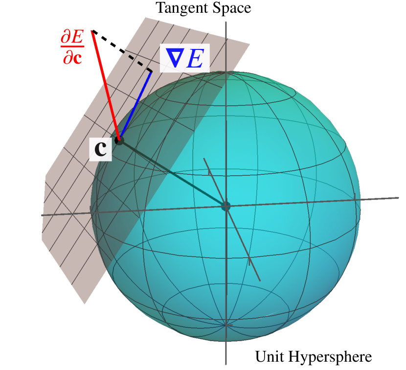
Figure 1: Geometric relationship between the position vector $\bm{c}$ (black) for a wave function constrained to the unit hypersphere, the global energy gradient in the full Hilbert space [red; Eq. (8)], and the local gradient in the tangent space [blue; Eq. (12)]

The stationary condition $\gradient E=\bm{0}$ requires that the global gradient Eq. (8) has no component in the tangent space. Therefore, it can only be satisfied if $\bm{H}\bm{c}$ is (anti)parallel to the position vector $\bm{c}$. This condition immediately recovers the expected eigenvector expression $\bm{H}\bm{c}_{k}=E_{k}\bm{c}_{k}$, where the eigenvalue $E_{k}$ is the exact energy of the $k$-th excited state with coefficient vector $\bm{c}_{k}$. As a result, each exact eigenstate is represented by two stationary points on the hypersphere that are related by a sign-change in the wave function (i.e., $\pm\bm{c}_{k}$ or, equivalently, $\pm\ket{\Psi_{k}}$). There are no other stationary points on the exact landscape.

The exact hypersphere can be compared to the constraint surface in HF theory, where the occupied orbitals represent the current position on a Grassmann manifold and occupied-virtual orbital rotations define the tangent basis vectors.Van Voorhis and Head-Gordon (2002); Edelman et al. (1998) In HF theory, the global gradient is given by $2\bm{F}\bm{C}_{\text{occ}}$, where $\bm{F}$ is the Fock matrix and $\bm{C}_{\text{occ(vir)}}$ are the occupied (virtual) orbital coefficients. Projection into the Grassmann tangent space then yields the local gradient as $2\bm{C}_{\text{vir}}^{\intercal}\bm{F}\bm{C}_{\text{occ}}^{\vphantom{\intercal}}$, which corresponds to the virtual–occupied block of the Fock matrix in the molecular orbital (MO) basis.Douady et al. (1980); Van Voorhis and Head-Gordon (2002); Chaban et al. (1997); Burton and Wales (2021) Therefore, in both HF theory and the exact formalism, optimisation of the energy requires the off-diagonal blocks of an effective Hamiltonian matrix to become zero such that the “occupied–virtual” coupling between orbitals or many-particle states vanishes.

II.3 Properties of exact stationary points

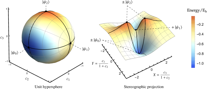
Figure 2: Left: Exact singlet electronic energy for H2 (STO-3G) at a bond length of $2\text{\,}\mathrm{\text{ $a_{0}$ }}$ constrained to the unit hypersphere. Right: Stereographic projection of the exact singlet energy using Eq. (20). Ground and excited states correspond to stationary points of the energy (black dots). The $-\ket{\Psi_{1}}$ state is at infinity in this representation. Each pair of stationary points is directly connected by a gradient extremal (black line) where the gradient is an eigenvector of the Hessian.

Stationary points on an energy landscape can be characterised as either minima, index-$k$ saddles, or maxima, depending on the number of downhill directions (or negative eigenvalues of the Hessian matrix). Following Ref. Edelman et al., 1998, the analytic Hessian $\mathbf{Q}$ of the exact energy constrained to the hypersphere is given by

$$\mathbf{Q}=\frac{\partial^{2}E}{\partial\bm{c}^{2}}-\quantity(\frac{\partial E}{\partial\bm{c}})^{\intercal}\bm{c}.$$ (13)

Taking the global second derivative in the full Hilbert space

$$\frac{\partial^{2}E}{\partial\bm{c}^{2}}=2\bm{H}$$ (14)

and exploiting the relationship

$$\quantity(\frac{\partial E}{\partial\bm{c}})^{\intercal}\bm{c}=2\,\bm{c}^{\intercal}\bm{H}\bm{c}=2E$$ (15)

allows the Hessian to be expressed as a shifted and rescaled Hamiltonian matrix

$$\mathbf{Q}=2\quantity(\bm{H}-E\,\bm{I}_{N}).$$ (16)

Projecting into the space spanned by the tangent vectors then gives the constrained local Hessian as an $(N-1)\times(N-1)$ matrix defined as

$$\widetilde{\mathbf{Q}}=2\,\bm{c}_{\bot}^{\intercal}\quantity(\bm{H}-E\,\bm{I}_{N})\,\bm{c}_{\bot}^{\vphantom{\intercal}},$$ (17)

where it should be remembered that $\bm{c}_{\bot}$ is an $N\times(N-1)$ matrix. This expression for the Hessian of a CI wave function is also obtained with the exponential transformation used in second-order MC-SCF approaches.Olsen et al. (1983); Roos et al. (2016)

The constrained Hessian allows the properties of exact stationary points to be recovered. Consider a constrained stationary point $\bm{c}_{k}$ corresponding to an exact eigenstate $\ket{\Psi_{k}}$ with energy $E_{k}$. To satisfy the completeness condition Eq. (10), the tangent basis vectors at this point must correspond to the remaining $(N-1)$ exact eigenstates. The local Hessian $\widetilde{\mathbf{Q}}$ is then simply the full Hamiltonian shifted by $E_{k}$ and projected into the basis of these $(N-1)$ exact eigenstates. As a result, the Hessian eigenvalues $\lambda_{i}$ are directly proportional to the excitation energies, giving

$$\lambda_{i}=2(E_{i}-E_{k})=2\Delta E_{ik},$$ (18)

where $E_{i}$ are the exact energies with $i\neq k$. Furthermore, the corresponding eigenvectors coincide with the position vectors $\bm{c}_{i}$ representing the remaining exact eigenstates $\ket{\Psi_{i}}$. Remarkably, this means that only the energy and second derivatives at an exact stationary point are required to deduce the electronic energies of the entire system. In other words, the full electronic energy spectrum is encoded in the local structure of the energy landscape around a single stationary point.

Now, at the stationary point $\bm{c}_{k}$ with energy $E_{k}$, the number of exact eigenstates that are lower in energy is equal to the excitation level $k$. The number of negative eigenvalues $\lambda_{i}=2\Delta E_{ik}$ is then equivalent to the excitation level. Significantly, there are only two minima on the exact energy landscape corresponding to positive and negative sign-permutations of the exact ground state, i.e. $\pm\ket{\Psi_{0}}$, and no higher-energy local minima. The $k$-th excited state forms a pair of index-$k$ saddle points that are also related by a sign-change in the wave function. The saddle-point nature of exact excited states was previously derived in the context of MC-SCF theory,Olsen et al. (1982, 1983); Golab et al. (1985, 1983) and has been described by Bacalis using local expansions around an excited state.N. C. Bacalis (2020) In fact, the Hessian index has been suggested as a means of targeting and characterising a particular MC-SCF excited state.Golab et al. (1983); Olsen et al. (1983) In contrast, here the stationary properties of exact excited states have been derived using only the differential geometry of functions under orthogonality constraints. As will be shown later, this differential geometry also reveals the global structure of the energy landscape and the connections between exact eigenstates.

These properties also apply within a particular symmetry subspace. For example, the first excited state of a given symmetry is an index-1 saddle on the energy landscape projected into the corresponding symmetry subspace, but may be a higher-index saddle on the full energy landscape. For a pair of degenerate eigenstates, the corresponding stationary points will have a zero Hessian eigenvalue and the corresponding eigenvector will interconvert the two states. Therefore, degenerate eigenstates form a flat continuum of stationary points on the exact energy landscape and any linear combination of the two states must also be a stationary point of the energy.

In Fig. 2, the structure of the exact energy landscape is illustrated for the singlet states of H2 at a bond length of $2\text{\,}\mathrm{\text{ $a_{0}$ }}$ using the STO-3G basis set.Hehre et al. (1969) An arbitrary spin-pure singlet wave function can be constructed as a linear combination of singlet configuration state functions to give

$$\ket{\Psi}=c_{1}\absolutevalue*{\sigma_{g}\bar{\sigma_{g}}}+\frac{c_{2}}{\sqrt{2}}\quantity(\absolutevalue*{\sigma_{g}\bar{\sigma_{u}}}+\absolutevalue*{\sigma_{u}\bar{\sigma_{g}}})+c_{3}\absolutevalue{\sigma_{u}\bar{\sigma_{u}}}.$$ (19)

Here, $\sigma_{g}$ and $\sigma_{u}$ are the symmetry-adapted MOs, and the absence (presence) of an overbar indicates an occupied high-spin (low-spin) orbital. A stereographic projection centred on $(c_{1},c_{2},c_{3})=(0,1,0)$ is used to highlight the topology of the energy landscape (Fig. 2: right panel), with new coordinates $X$ and $Y$ defined as

$$X=\frac{c_{3}}{1+c_{2}}\quad\text{and}\quad Y=\frac{c_{1}}{1+c_{2}}.$$ (20)

The ground and excited states (black dots) form stationary points constrained to the hypersphere (Fig. 2: left panel) with the global minima representing the ground state, index-1 saddles representing the first excited state, and the global maxima representing the second excited state (Fig. 2: right panel). At the index-1 saddle, the downhill directions connect the two sign-permutations of the ground-state wave function, while the two uphill directions connect sign-permutations of the second excited singlet state.

II.4 Gradient extremals on the electronic energy surface

Energy landscapes can also be characterised by the pathways that connect stationary points. For molecular potential energy surfaces, pathways can be interpreted as reaction trajectories between stable molecular structures, with saddle points representing reactive transition states.Wales (2004) However, unlike stationary points, these pathways do not have a unique mathematical definition. On the exact electronic energy landscape, gradient extremals represent the most obvious pathways between stationary points. A gradient extremal is defined as a set of points where the gradient is either maximal or minimal along successive energy-constant contour lines.Hoffman et al. (1986) For the contour line with energy $E_{\text{c}}$, these points can be identified by the constrained optimisationSzabo and Ostlund (1989)

$$\begin{split}\frac{\partial}{\partial\bm{c}}\quantity[\absolutevalue{\gradient E}^{2}-2\lambda\quantity(E-E_{c})]=2\quantity[\widetilde{\mathbf{Q}}\cdot\gradient E-\lambda\gradient E]=0.\end{split}$$ (21)

Therefore, gradient extremals are pathways where the local gradient is an eigenvector of the local Hessian, i.e.

$$\widetilde{\mathbf{Q}}(\bm{c})\,\gradient E(\bm{c})=\lambda(\bm{c})\gradient E(\bm{c}).$$ (22)

These pathways propagate away from each stationary point along the “normal mode” eigenvectors of the Hessian and provide the softest or steepest ascents from a minimum.Hoffman et al. (1986)

On the exact FCI landscape, gradient extremals directly connect each pair of stationary points, as illustrated by the black lines in Fig. 2. Each extremal corresponds to the geodesic connecting the two stationary points along the surface of the hypersphere. The wave function along these pathways is only a linear combination of the two eigenstates at each end of the path. Therefore, gradient extremals provide a well-defined route along which a ground-state wave function can be continuously evolved into an excited-state wave function, or vice-versa. Furthermore, as a gradient extremal moves from the lower-energy to the higher-energy stationary point, the corresponding Hessian eigenvalue $\lambda(\bm{c})$ changes from positive to negative. This leads to an inflection point with $\lambda(\bm{c})=0$ exactly halfway along each gradient extremal where the wave function is an equal combination of the two exact eigenstates. These inflection points are essential for understanding the structure of the variance optimisation landscape in Section II.5.

II.5 Structure of the exact variance landscape

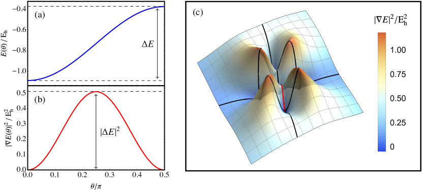
Figure 3: Energy square-gradient for the singlet states of H2 (STO-3G) at a bond length of $2\text{\,}\mathrm{\text{ $a_{0}$ }}$. (a) Energy along the gradient extremal connecting the ground and first excited singlet state. (b) Square-gradient of the energy along the gradient extremal connecting the ground and first excited singlet state. (c) Square-gradient landscape for singlet wave functions in H2 (STO-3G), with gradient extremals (black) connecting the physical minima. The gradient extremal plotted in (b) is highlighted in red.

The accuracy of a general point on the exact energy landscape can be assessed using the square-magnitude of the local gradient, defined using Eq. (12) as

$$\absolutevalue{\gradient E(\bm{c})}^{2}=4\,\bm{c}^{\intercal}\bm{H}\bm{c}_{\bot}^{\vphantom{\intercal}}\bm{c}_{\bot}^{\intercal}\bm{H}\bm{c}.$$ (23)

Since all stationary points are minima of the squared-gradient with $\absolutevalue{\gradient E(\bm{c})}^{2}=0$, minimising this objective function has been proposed as a way of locating higher-index saddle points in various contexts.Broderix et al. (2000); Angelani et al. (2000); Hait and Head-Gordon (2020) For the electronic structure problem, exploiting the relationship between the tangent- and normal-space projectors [Eq. (10)] allows Eq. (23) to be expressed using only the position vector $\bm{c}$ as

$$\absolutevalue{\gradient E}^{2}=4\,\bm{c}^{\intercal}\bm{H}\quantity(\bm{I}_{N}-\bm{c}\bm{c}^{\intercal})\bm{H}\bm{c}.$$ (24)

Further expanding this expression gives

$$\absolutevalue{\gradient E}^{2}=4\quantity(\bm{c}^{\intercal}\bm{H}^{2}\bm{c}-\quantity(\bm{c}^{\intercal}\bm{H}\bm{c})^{2}),$$ (25)

which can be recognised as four times the Hamiltonian variance, i.e.

$$\absolutevalue{\gradient E}^{2}=4\matrixelement*{\Psi}{(\mathcal{H}-E)^{2}}{\Psi}.$$ (26)

While variance optimisation has previously inspired the development of excited-state variational principles,Messmer (1969); Shea and Neuscamman (2017); Pineda Flores and Neuscamman (2019); Cuzzocrea et al. (2020); Ye et al. (2017); Ye and Van Voorhis (2019) these approaches have generally been motivated by the fact that exact eigenstates of $\mathcal{H}$ also have zero variance. In contrast, the relationship between the variance and $\absolutevalue{\gradient E}^{2}$ provides a purely geometric motivation behind searching for excited states in this way, derived from the structure of the exact energy landscape. Hait and Head-Gordon alluded to a relationship of this type by noticing similarities between the equations for SCF square-gradient minimisation and optimising the SCF variance.Hait and Head-Gordon (2020)

By connecting the squared-gradient of the energy to the variance, the exact energy landscape can be used to deduce the structure of the variance optimisation landscape. Exact eigenstates form minima on the square-gradient landscape with $\absolutevalue{\gradient E}^{2}=0$. However, the square-gradient can have additional non-zero stationary points corresponding to local minima, higher-index saddle points, or local maxima.Doye and Wales (2002, 2003) These “non-stationary” points do not represent stationary points of the energy, but they provide important information about the structure of the square-gradient landscape away from exact eigenstates. In particular, a stationary point of $\absolutevalue{\gradient E}^{2}$ with $\gradient E\neq\bm{0}$ can only occur when the local gradient is an eigenvector of the Hessian with a zero eigenvalue, $\widetilde{\mathbf{Q}}(\bm{c})\,\gradient E(\bm{c})=\bm{0}.$Doye and Wales (2002, 2003) Non-stationary points therefore occur on the gradient extremals described in Section II.4 and correspond to the inflection points exactly halfway between each pair of eigenstates.

Since gradient extremals only connect two eigenstates, the value of $\absolutevalue{\gradient E}^{2}$ at these non-stationary points can be obtained by parametrising the wave function as

$$\ket{\Psi(\theta)}=\cos\theta\ket*{\Psi_{i}}+\sin\theta\ket*{\Psi_{j}}.$$ (27)

The energy and square-gradient are then given by

$$E(\theta) =E_{i}+\Delta E_{ji}\,\sin^{2}\theta,$$ (28a)

$$\absolutevalue{\gradient E(\theta)}^{2} =\Delta E_{ji}^{2}\,\sin^{2}2\theta,$$ (28b)

where $0\leq\theta\leq\pi/2$ and $\Delta E_{ji}=E_{j}-E_{i}$. There are only two stationary points of the energy along each pathway, corresponding to $\absolutevalue{\gradient E}^{2}=0$ at $\theta=0$ and $\pi/2$, as illustrated for the gradient extremal connecting the ground and first excited singlet states of H2 (STO-3G) in Fig. 3a. In contrast, the square-gradient has an additional stationary point at the inflection point $\theta=\pi/4$ with $\absolutevalue{\gradient E}^{2}=\Delta E_{ji}^{2}$ (see Fig. 3b). This point corresponds to an unphysical maximum of $\absolutevalue{\gradient E}^{2}$ along the gradient extremal and the height of this barrier depends on the square of the energy difference between the two states. Therefore, the exact square-gradient (or variance) landscape contains exact minima separated by higher-variance stationary points that form barriers at the inflection points of the energy, with the height of each barrier directly proportional to the square of the energy difference between the connected eigenstates. The lowest square-gradient barrier always connects states that are adjacent in energy to form an index-1 saddle point, while barriers connecting states that are not adjacent in energy form higher-index saddle points of $\absolutevalue{\gradient E}^{2}$. This structure of the exact square-gradient landscape is illustrated for the singlet states of H2 in Fig. 3c.

Connecting the variance to the exact energy square-gradient reveals that the general structure of the variance optimisation landscape is universal and completely determined by the energy difference between exact eigenstates. Systems with very small energy gaps will have low barriers between exact variance minima, while systems with well-separated energies will have high-variance barriers. This structure may also play a role in explaining the convergence behaviour of variance minimisation approaches, as discussed in Section IV.

III Understanding Approximate Wave Functions

III.1 Differential geometry on the exact energy landscape

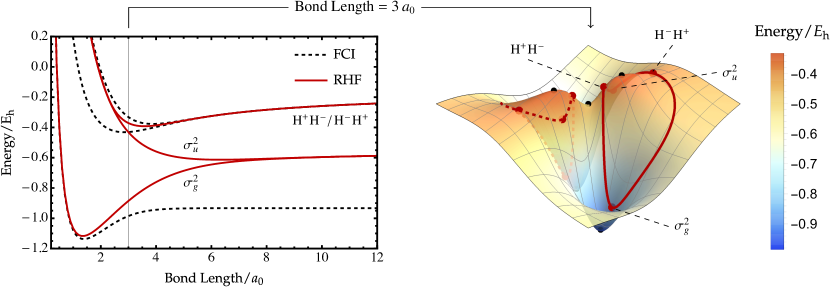
Figure 4: The space of possible RHF wave functions forms a one-dimensional submanifold (right panel; red curve) on the exact singlet energy surface for H2 (STO-3G) with a bond length of $3\text{\,}\mathrm{\text{ $a_{0}$ }}$. Multiple RHF solutions (left panel) correspond to constrained stationary points on the RHF manifold (right panel; red dots). The sign-permuted RHF wave functions are denoted by a dashed red curve (red panel).

Any normalised wave function approximation $\ket*{\tilde{\Psi}(\bm{t})}$ with variational parameters $\bm{t}$ can be represented as a point on the exact hypersphere using a linear expansion in the many-particle basis

$$\ket*{\tilde{\Psi}(\bm{t})}=\sum_{I=1}^{N}\tilde{c}_{I}(\bm{t})\ket{\Phi_{I}}.$$ (29)

Like the exact wave function, this expansion is invariant to the particular choice of orthogonal basis determinants. Since the number of parameters $t_{i}$ is generally smaller than the Hilbert space size, the approximate wave functions form a constrained submanifold of the exact hypersphere. The structure of this approximate submanifold is implicitly defined by the mathematical form of the parametrisation. Geometrically, the approximate energy is given as

$$E(\bm{t})=\tilde{\bm{c}}(\bm{t})^{\intercal}\,\bm{H}\,\tilde{\bm{c}}(\bm{t}),$$ (30)

and the constrained local gradient is defined as

$$\quantity(\widetilde{\gradient}E)_{i}=\frac{\partial E(\bm{t})}{\partial t_{i}}=2\,\quantity(\frac{\partial\tilde{\bm{c}}(\bm{t})}{\partial t_{i}})^{\intercal}\bm{H}\,\tilde{\bm{c}}(\bm{t}).$$ (31)

Here, the partial derivatives of the coefficient vector define the local tangent basis of the approximate submanifold, representing the ket vectors

$$\ket*{\eta_{i}}=\partialderivative{t_{i}}\ket*{\tilde{\Psi}(\bm{t})}.$$ (32)

In analogy with the exact wave function, the approximate local gradient corresponds to the global gradient [Eq. (8)] projected into the space spanned by the approximate tangent vectors [Eq. (32)]. Optimal stationary points of the approximate energy then occur when $\widetilde{\gradient}E=\bm{0}$.

The HF approach illustrates how well-known approximate stationary conditions can be recovered with this geometric perspective. Although HF theory is usually presented as an iterative self-consistent approach,Roothaan (1951); Hall (1951) the HF wave function can also be parametrised using an exponential transformation of a reference determinant to giveThouless (1960); Douady et al. (1980)

$$\ket{\Phi(\bm{\kappa})}=\exp(\hat{\kappa})\ket{\Phi_{0}}.$$ (33)

Here, $\hat{\kappa}$ is a unitary operator constructed from closed-shell single excitations and de-excitations, represented in second-quantisation asHelgaker et al. (2000)

$$\hat{\kappa}=\sum_{ai}\kappa_{ai}\quantity(a_{a}^{\dagger}a_{i}^{\vphantom{\dagger}}-a_{i}^{\dagger}a_{a}^{\vphantom{\dagger}})$$ (34)

where $\kappa_{ai}$ are the variable parameters. The tangent vectors at $\bm{\kappa}=\bm{0}$ correspond to the singly-excited configurations, i.e.

$$\ket{\eta_{ai}}=\left.\frac{\partial\ket{\Phi(\bm{\kappa})}}{\kappa_{ai}}\right\rvert_{\bm{\kappa}=\bm{0}}=\ket{\Phi_{i}^{a}}.$$ (35)

These approximate tangent vectors span a subspace of the exact tangent space on the full hypersphere. Using Eq. (31), the local HF gradient is then given byDouady et al. (1980); Van Voorhis and Head-Gordon (2002)

$$\quantity(\widetilde{\gradient}E)_{ai}=2\matrixelement*{\Phi_{i}^{a}}{\mathcal{H}}{\Phi_{0}}=2F_{ai},$$ (36)

which corresponds to twice the virtual-occupied components of the Fock matrix in the MO basis. As expected, the stationary condition $\widetilde{\gradient}E=\bm{0}$ recovers Brillouin’s theorem for HF convergence.Szabo and Ostlund (1989)

III.2 Multiple Hartree–Fock solutions

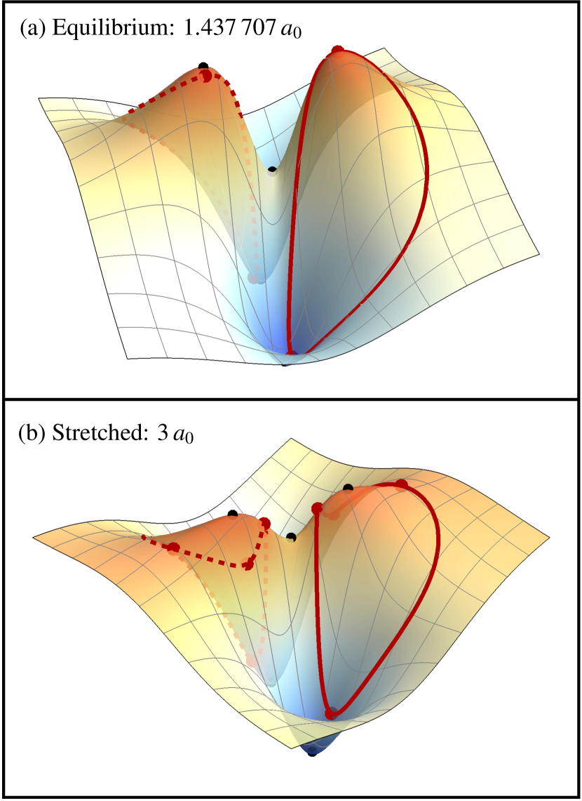
Figure 5: Mapping between the RHF submanifold (solid red line) and the exact singlet energy surface for H2 (STO-3G) at (a) the equilibrium bond length $1.437\,707\text{\,}\mathrm{\text{ $a_{0}$ }}$ and (b) a stretched geometry $3\text{\,}\mathrm{\text{ $a_{0}$ }}$. Sign-permuted RHF wave functions are denoted by dashed red curves.

Although the HF wave function has fewer parameters than the exact wave function, there can be more HF stationary points than exact eigenstates.Stanton (1968); Burton et al. (2018) For example, in dissociated H2 with a minimal basis set, there are four closed-shell restricted HF (RHF) solutions and only three exact singlet states.Burton et al. (2018) In contrast to the exact eigenstates, there can also be multiple HF solutions with the same Hessian index, although this index generally increases with energy.Burton et al. (2018) Furthermore, HF solutions do not necessarily exist for all molecular geometries and can disappear at so-called “Coulson–Fischer” points.Coulson and Fischer (1949); Slater (1951); Thom and Head-Gordon (2008); Huynh and Thom (2020); Burton et al. (2018); Burton and Wales (2021) These phenomena can all be understood through the geometric mapping between the approximate HF submanifold and the exact energy landscape.

Consider the RHF approximation for the singlet states of H2 (STO-3G). Only two RHF solutions exist at the equilibrium geometry, while an additional higher-energy pair of degenerate solutions emerge in the dissociation limit, as shown in the left panel of Fig. 4 (see Ref. Burton et al., 2018 for further details). In this system, the RHF submanifold forms a continuous one-dimensional subspace of the exact energy surface, illustrated by the red curve in Fig. 4 (right panel). This submanifold includes all possible closed-shell Slater determinants for the system and is fixed by the wave function parametrisation. Approximate solutions then correspond to constrained stationary points of the energy along the RHF submanifold, which occur when the global energy gradient has no component parallel to the red curve. The existence and properties of these solutions is completely determined by the mapping between the RHF submanifold and the exact energy landscape.

At bond lengths near the equilibrium structure of H2 (STO-3G), the RHF submanifold extends relatively close to the exact global minimum and maximum, as illustrated in Fig. 5a. This mapping results in only two constrained stationary points, the global minimum and maximum of the RHF energy, which correspond to the symmetry-pure $\sigma_{g}^{2}$ and $\sigma_{u}^{2}$ configurations respectively. Notably, the RHF $\sigma_{u}^{2}$ global maximum represents a doubly-excited state that cannot be accurately described by TD-HF or CIS.Burke et al. (2005) However, the RHF submanifold cannot get sufficiently close to the exact open-shell singlet state to provide a good approximation, and there is no stationary point representing this single excitation.

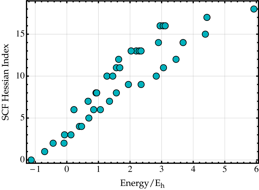
Figure 6: Comparison of the energy and SCF Hessian index computed for the orbital-optimised excited configurations of H2 (cc-pVDZDunning Jr. (1989)) at $R=$1.437\,707\text{\,}\mathrm{\text{ $a_{0}$ }}$$ using unrestricted HF.

As the H-H bond is stretched towards dissociation, the exact energy landscape on the hypersphere changes while the RHF submanifold remains fixed by the functional form of the approximate wave function. Therefore, the exact energy evolves underneath the RHF submanifold, creating changes in the approximate energy that alter the properties of the constrained stationary points. For example, at a sufficiently large bond length, the RHF submanifold no longer provides an accurate approximation to the exact global maximum and instead encircles it to give two local maxima and a higher-energy local minimum of the RHF energy (Fig. 5b). These local maxima represent the spatially-symmetry-broken RHF solutions that tend towards to the ionic dissociation limit (left panel in Fig. 4), while the higher-energy local minimum represents the $\sigma_{u}^{2}$ configuration. Combined with the global minimum, this gives a total of four RHF solutions, in contrast to only three exact singlet states. Consequently, we find that the number of RHF solutions can exceed the number of exact eigenstates because the RHF submanifold is a highly constrained non-linear subspace of the exact energy landscape. Furthermore, it is the structure of this constrained subspace that creates a high-energy local minimum at dissociation, while the exact energy landscape has no local minima at any geometry.

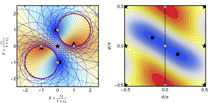
Figure 7: Left: RHF (solid and dashed red curves) and ESMF (blue mesh) constrained submanifolds superimposed on a stereographic projection [see Eq. (20)] of the exact singlet energy landscape for H2 (STO-3G) at a bond length of $R=$1.437\,707\text{\,}\mathrm{\text{ $a_{0}$ }}$$. Exact stationary points and RHF solutions occur at the black and red dots respectively. Right: The ESMF energy for singlet H2 (STO-3G) as a function of the wave function parameters [see Eq. (40)]. Black and grey symbols indicate stationary points of the ESMF or RHF energy respectively, and the RHF submanifold corresponds to $\theta=0$ (dashed black line).

Finally, for real-valued HF wave functions, the Hessian of the approximate energy is computed using the second derivativesSeeger and Pople (1977)

$$\frac{\partial^{2}E(\bm{t})}{\partial t_{ia}\partial t_{jb}}=2\,\Big{(}\matrixelement*{\Phi_{i}^{a}}{\mathcal{H}-E}{\Phi_{j}^{b}}+\matrixelement*{\Phi}{\mathcal{H}-E}{\Phi_{ij}^{ab}}\Big{)},$$ (37)

where now open-shell orbital rotations are now allowed. To investigate how the HF Hessian index changes with energy, the unrestricted excited configurations obtained from the ground-state RHF orbitals of H2 (cc-pVDZDunning Jr. (1989)) at $R~{}=~{}$1.437\,707\text{\,}\mathrm{\SIUnitSymbolAngstrom}$$ were optimised using the initial maximum overlap methodBarca et al. (2018) in Q-Chem 5.4.Epifanovsky et al. (2021) The corresponding Hessian indices are plotted against the optimised energy in Fig. 6. Similarly to the exact eigenstates, there is a general increase in the Hessian index at higher energies. However, unlike the exact eigenstates, the approximate Hessian index does not increase monotonically with the energy. These results strengthen the conclusion of Ref. Burton and Wales, 2021 that approximate HF excited states are generally higher-index saddle points of the energy.

III.3 Excited-state mean-field theory

While multiple HF solutions are relatively well understood, the energy landscape of orbital-optimised post-HF wave functions remains less explored. The simplest excited-state extension of HF theory is the CIS wave function,Foresman et al. (1992); Dreuw and Head-Gordon (2005) constructed as a linear combination of singly-excited determinants. CIS generally provides a qualitatively correct description of singly excited states, but it is less reliable for multiconfigurational or charge transfer excitations.Dreuw and Head-Gordon (2005) The systematic overestimate of CIS for charge transfer excitations can be attributed to the absence of orbital relaxation effects.Subotnik (2011) Therefore, to improve this description, the orbitals and CI coefficients can be simultaneously optimised to give the state-specific excited-state mean-field (ESMF) wave function, defined for singlet states asShea and Neuscamman (2018)

$$\ket{\Psi_{\text{ESMF}}}=\exp(\hat{\kappa})\quantity[c_{0}+\frac{1}{\sqrt{2}}\sum_{ia}c_{ia}\quantity(a^{\dagger}_{a}a^{\vphantom{\dagger}}_{i}+a^{\dagger}_{\bar{a}}a^{\vphantom{\dagger}}_{\bar{i}})]\ket{\Phi_{0}}.$$ (38)

Here, the reference determinant is retained in the expansion and orbital rotations are parametrised by the unitary rotation defined in Eq. (34). In recent years, efficient optimisation of this ansatz has been successfully applied to charge transfer and core excitations.Shea and Neuscamman (2018); Zhao and Neuscamman (2020); Hardikar and Neuscamman (2020); Garner and Neuscamman (2020) Alternative approaches to include orbital relaxation effects in CIS using perturbative corrections have also been investigated.Liu et al. (2012, 2013); Liu and Subotnik (2014)

Geometrically, the single excitations for any closed-shell reference determinant define the tangent vectors to the RHF submanifold. Therefore, the orbital-optimised ESMF submanifold contains the RHF wave functions and all points that lie in the combined tangent spaces of the RHF submanifold, as illustrated for the singlet states of H2 (STO-3G) in Fig. 7 (left panel). Like multiple RHF solutions, state-specific ESMF solutions correspond to stationary points of the energy constrained to the ESMF wave function manifold.

The ESMF wave function for singlet H2 (STO-3G) can be constructed by parametrising the occupied and virtual molecular orbitals with a single rotation angle $\phi$ as

$$\psi_{1}(\bm{r}) =\cos\phi\,\sigma_{g}(\bm{r})+\sin\phi\,\sigma_{u}(\bm{r}),$$ (39a)

$$\psi_{2}(\bm{r}) =\cos\phi\,\sigma_{u}(\bm{r})-\sin\phi\,\sigma_{g}(\bm{r}).$$ (39b)

and defining the normalised singlet CI expansion with a second rotation angle $\theta$ to give

$$\ket{\Psi_{\text{ESMF}}}=\cos\theta\,\absolutevalue*{\psi_{1}\bar{\psi}_{1}}+\sin\theta\,\frac{\absolutevalue*{\psi_{1}\bar{\psi}_{2}}+\absolutevalue*{\psi_{2}\bar{\psi}_{1}}}{\sqrt{2}}.$$ (40)

The corresponding energy landscape at the equilibrium bond length $R=$1.437\,707\text{\,}\mathrm{\text{ $a_{0}$ }}$$ is shown in Fig. 7 (right panel) as a function of $\theta$ and $\phi$, with the RHF approximation indicated by the dashed black line at $\theta=0$. Stationary points representing the exact open-shell singlet state occur at $(\theta,\phi)=(\pm\frac{\pi}{2},0)$ and $(\pm\frac{\pi}{2},\pm\frac{\pi}{2})$, denoted by black stars, with optimal orbitals that correspond to $\sigma_{g}(\bm{r})$ and $\sigma_{u}(\bm{r})$. In common with the exact energy landscape, these open-shell singlet solutions form index-1 saddle points of the singlet energy. On the other hand, the local maximum representing the double excitation has no contribution from the single excitations and reduces to the closed-shell $\sigma_{u}^{2}$ RHF solution (grey diamonds). This lack of improvement beyond RHF can be understood from the structure of the singlet ESMF submanifold: the exact double excitation is encircled by the RHF submanifold and therefore cannot be reached by any of the tangent spaces to the RHF wave function (Fig. 7: left panel).

However, the most surprising observation from Fig. 7 is not the higher-energy stationary points of the ESMF energy, but the location of the global minimum. Counter-intuitively, the RHF ground state becomes an index-1 saddle point of the ESMF energy (grey circles) and there is a lower-energy solution at $(\theta,\phi)=(\pm 0.5026,\mp 0.3304)$ that corresponds to the exact ground state (black squares). This lower-energy solution occurs because rotating the orbitals away from an optimal HF solution breaks Brillioun’s condition and introduces new coupling terms between the reference and singly-excited configurations that allow the energy to be lowered below the RHF minimum. Since the RHF ground state is stationary with respect to both orbital rotations and the introduction of single excitations, this cooperative effect can only occur when the orbital and CI coefficients are optimised simultaneously. Furthermore, the combined orbital and CI Hessian is required to diagnose the RHF ground state as a saddle point of the ESMF energy, highlighting the importance of considering the full parametrised energy landscape.

The existence of an ESMF global minimum below the RHF ground state challenges the idea that CIS-based wave functions are only useful for approximating excited states. From a practical perspective, current ESMF calculations generally underestimate excitation energies because the multiconfigurational wave function used for the excited state can capture some electron correlation, while the single-determinant RHF ground state remains completely uncorrelated.Shea and Neuscamman (2018) Although CIS is often described as an uncorrelated excited-state theory, the wave function is inherently multi-configurational and becomes correlated when the first-order density matrix is not idempotent.Surjan (2007) These circumstances generally correspond to excitations with more than one dominant natural transition orbital.Plasser (2016) Therefore, it is not too surprising that the ESMF global minimum can provide a correlated representation of the ground state. As a result, using state-specific ESMF wave functions for both the ground and excited states should provide a more balanced description of an electronic excitation.

Since the global minimum is exact across all H2 bond lengths, orbital-optimised ESMF may also provide an alternative reference wave function for capturing static correlation in single-bond breaking processes. The success of this ansatz can be compared to the spin-flip CIS (SF-CIS) approach, where the CI expansion is constructed using spin-flipping excitations from a high-spin reference determinant.Krylov (2001) SF-CIS gives an accurate description of the H2 ground state because single spin-flip excitations from an open-shell $\sigma_{g}\sigma_{u}$ reference produce both the $\sigma_{g}^{2}$ and $\sigma_{u}^{2}$ configurations. In contrast, the ESMF global minimum contains a closed-shell reference determinant with symmetry-broken orbitals, as shown in Fig. 8. These orbitals resemble the $\sigma_{g}$ and $\sigma_{u}$ MOs at short geometries [Fig. 8(a)–(b)] where the reference determinant $|\psi_{1}\bar{\psi}_{1}|$ dominates the ESMF wave function. As the bond is stretched, the optimised orbitals localise on opposite H atoms to give an ionic reference state [Fig. 8(e)–(f)] and the single excitations correspond to the localised configurations required for the diradical ground state.

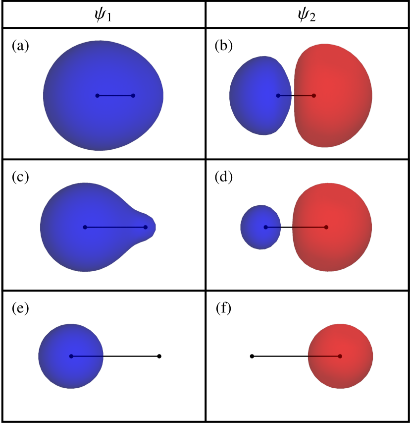
Figure 8: Spatial orbitals for the optimised ESMF ground state of H2 (STO-3G) at bond lengths of (a)–(b) $1.437\,707\text{\,}\mathrm{\text{ $a_{0}$ }}$, (c)–(d) $3.0\text{\,}\mathrm{\text{ $a_{0}$ }}$, and (e)–(f) $6.0\text{\,}\mathrm{\text{ $a_{0}$ }}$, plotted with an isosurface value of $\pm 0.05$. The reference configuration corresponds to $|\psi_{1}\bar{\psi}_{1}|$ with the ESMF wave function defined in Eq. (40).

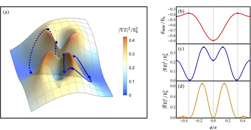
Figure 9: (a) Exact square-gradient landscape for singlet H2 (STO-3G) at a bond length of $3\text{\,}\mathrm{\text{ $a_{0}$ }}$. Restricted $\sigma$-SCF solutions identified using variance optimisation are equivalent to constrained stationary points (blue dots) on the single-determinant subspace (blue curve) and its sign-related copy (dashed blue curve). (b) RHF energy as a function of the single orbital rotation angle $\phi$ [see Eq. (42)]. (c) Exact square-gradient of RHF wave functions with stationary points corresponding to $\sigma$-SCF solutions. (d) Square-magnitude of the constrained RHF energy gradient, with minima corresponding to RHF energy stationary points.

III.4 Unphysical solutions in variance optimisation

Approximate state-specific variance minimisation can also be considered as an optimisation of the exact variance constrained to the approximate wave function submanifold. Variance minimisation is increasingly being applied to target excited states because it turns the optimisation of higher-energy stationary points into a minimisation problemMessmer (1969); Shea and Neuscamman (2017); Pineda Flores and Neuscamman (2019); Ye et al. (2017); Ye and Van Voorhis (2019); David et al. (2021) and is easily applied for correlated wave functions using VMC.Otis et al. (2020); Cuzzocrea et al. (2020) In practice, these algorithms often use the folded-spectrum objective functionWang and Zunger (1994)

$$\Omega=\frac{\matrixelement*{\tilde{\Psi}}{(\mathcal{H}-\omega)^{2}}{\tilde{\Psi}}}{\innerproduct*{\tilde{\Psi}}{\tilde{\Psi}}}$$ (41)

to target an excited state with an energy near $\omega$, before self-consistently updating $\omega$ until a variance stationary point is reached with $\omega=E$.Ye et al. (2017); Ye and Van Voorhis (2019); Cuzzocrea et al. (2020) However, the structure of the variance landscape for approximate wave functions, and the properties of its stationary points, are relatively unexplored.

Since the variance is equivalent to the exact square-gradient $\absolutevalue{\gradient E}^{2}$, this landscape can be investigated using the mapping between an approximate wave function and the exact square-gradient landscape derived in Sec. II.5. Consider the RHF approximation in H2 (STO-3G) with the doubly-occupied orbital parametrised as

$$\psi(\bm{r})=\cos\phi\,\sigma_{g}(\bm{r})+\sin\phi\,\sigma_{u}(\bm{r}).$$ (42)

Variance optimisation for HF wave functions has been developed by Ye et al. as the iterative $\sigma$-SCF method, which uses a variance-based analogue of the Fock matrix.Ye et al. (2017); Ye and Van Voorhis (2019) In Figure 9a, the RHF submanifold is shown as a subspace of the exact singlet square-gradient landscape at $R=$3\text{\,}\mathrm{\text{ $a_{0}$ }}$$, with optimal $\sigma$-SCF solutions corresponding to the constrained stationary points. Since the RHF approximation cannot reach any exact eigenstates in this system, the square-gradient is non-zero for all RHF wave functions and there is no guarantee that the $\sigma$-SCF solutions coincide with stationary points of the constrained energy. This feature is illustrated in Figs. 9b and 9c, where the energy and square-gradient are compared for the occupied orbital defined in Eq. (42). There are three constrained minima of the square-gradient for these RHF wave functions. The first, at $\phi=0$ corresponds to the $\sigma_{g}^{2}$ RHF ground state, while the other two represent ionic configurations that are similar, but not identical, to the local maxima of the RHF energy.Ye et al. (2017) However, the $\sigma_{u}^{2}$ configuration, which forms a local minimum of the RHF energy, becomes a constrained local maximum of the energy square-gradient.

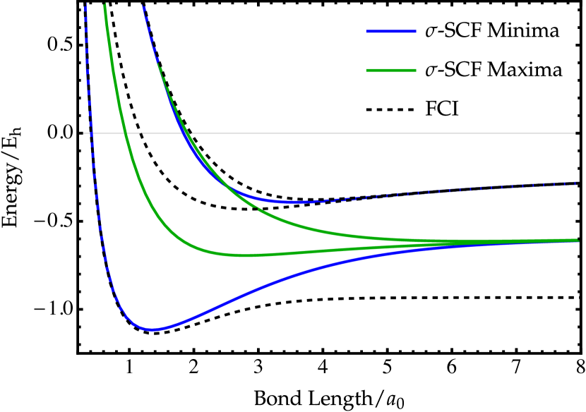
Figure 10: Energy of restricted $\sigma$-SCF solutions corresponding to constrained stationary points of the variance in H2 (STO-3G), including local minima (blue) and maxima (green). Exact singlet energies are shown for comparison (black dashed).

Energies corresponding to the complete set of RHF variance stationary points for H2 (STO-3G) are shown in Fig. 10, with variance minima and maxima denoted by blue and green curves respectively. These solutions closely mirror the low-energy $\sigma$-SCF states identified using the 3-21G basis set in Ref. Ye et al., 2017. Despite becoming a local maximum of the variance at large bond lengths, the $\sigma$-SCF approach identifies the $\sigma_{u}^{2}$ solution at all geometries.Ye et al. (2017) Therefore, iterative methods such as $\sigma$-SCF must be capable of converging onto higher-index stationary points of the variance. However, not all higher-index stationary points correspond to physically meaningful solutions. For example, an additional degenerate pair of $\sigma$-SCF maxima can be found at all bond lengths in H2, with an energy that lies between the $\sigma_{g}^{2}$ and $\sigma_{u}^{2}$ solutions. These unphysical maxima exist where the RHF manifold passes over the square-gradient barriers created by non-stationary points on the exact energy landscape (see Fig. 9a). The high non-convexity of the exact square-gradient landscape means that these unphysical higher-index stationary points of the variance are likely to be very common for approximate wave functions.

As an alternative to variance minimisation, excited state-specific wave functions can be identified by directly searching for points where the approximate local gradient becomes zero $\widetilde{\gradient}E=\bm{0}$. For example, Shea and Neuscamman introduced an approach that modifies the objective function Eq. (41) using Lagrange multipliers to ensure that the approximate local gradient vanishes at a solution.Shea and Neuscamman (2018) Alternatively, Hait and Head-Gordon proposed the square-gradient minimisation (SGM) algorithm that directly minimises the square-magnitude of the local electronic gradient $\absolutevalue*{\widetilde{\gradient}E}^{2}$.Hait and Head-Gordon (2020) While the SGM approach is closely related to minimising the exact variance, all stationary points of the approximate energy now become minima of local square-gradient with $\absolutevalue*{\widetilde{\gradient}E}^{2}=0$, as shown for the RHF wave functions of H2 (STO-3G) in Fig. 9d. Unphysical square-gradient stationary points, such as those resembling the RHF variance maxima in Fig. 9c, can then be easily identified with $\absolutevalue*{\widetilde{\gradient}E}^{2}\neq 0$. However, since the approximate energy can have more stationary points than the exact energy, there will be more non-stationary points of $\absolutevalue*{\widetilde{\gradient}E}^{2}$ corresponding to inflection points between stationary states of the approximate energy (cf. Fig. 9a and 9d). These additional non-stationary points will make the approximate $\absolutevalue*{\widetilde{\gradient}E}^{2}$ landscape even more non-convex than the constrained variance landscape, which can make numerical optimisation increasingly difficult.

IV Implications for Optimisation Algorithms

We have seen that the exact energy landscape for real wave functions has only two minima, corresponding to negative and positive sign-permutations of the exact ground state. In addition, there is only one sign-permuted pair of index-$k$ saddle points corresponding to the $k$-th excited state. On the contrary, approximate methods may have higher-energy local minima and multiple index-$k$ saddle points, although the maximum Hessian index is dictated by the number of approximate wave function parameters. These higher-energy local minima result from the wave function constraints introduced by lower-dimensional approximations.

The structure of the exact energy landscape highlights the importance of developing excited state-specific algorithms that can converge onto arbitrary saddle points of the energy. Any type of stationary point can be identified using iterative techniques that modify the SCF procedure, including the maximum overlap methodGilbert et al. (2008); Besley et al. (2009) and state-targeted energy projection.Carter-Fenk and Herbert (2020) In addition, modified quasi-Newton optimisation of the SCF energyLevi et al. (2020, 2020) should perform well, while state-specific CASSCFTran et al. (2019); Tran and Neuscamman (2020) may also benefit from similar second-order optimisation. Alternatively, modified eigenvector-following may allow excited states with a particular Hessian index to be targeted.Doye and Wales (2002); Wales and Doye (2003); Burton and Wales (2021) However, methods that search for local minima of the energy, including SCF metadynamicsThom and Head-Gordon (2008) and direct minimisation,Van Voorhis and Head-Gordon (2002) will perform less well for excited states and are better suited to locating the global minimum or symmetry-broken solutions.

In addition, the structure of the energy square-gradient landscape elucidates the challenges faced by variance optimisation approaches. Each exact eigenstate forms a minimum of the variance and minima adjacent in energy are separated by an index-1 saddle point with height proportional to the square of the corresponding energy difference.

Low barriers on the exact variance landscape offer a new perspective on the convergence drift observed in excited-state VMC calculations.Cuzzocrea et al. (2020); Otis et al. (2020) In Ref. Cuzzocrea et al., 2020, variance optimisation was found to drift away from the intended target state defined by the initial guess, passing through eigenstates sequentially in energy until converging onto the state with the lowest variance. By definition, a deterministic minimisation algorithm cannot climb over a barrier to escape a variance minimum. However, the statistical uncertainty of stochastic VMC calculations means that they can climb a variance barrier if the height is sufficiently low. Essentially, the variance barrier becomes “hidden” by statistical noise. The index-1 variance saddle points connecting states adjacent in energy may then explain why the optimisation drifts through eigenstates sequentially in energyCuzzocrea et al. (2020) and why this issue is more prevalent in systems with small energy gaps.Otis et al. (2020) Alternatively, the VMC wave function may simply not extend far enough into the exact variance basin of attraction of the target state to create an approximate local minimum. However, the use of highly-sophisticated wave functions in Ref. Cuzzocrea et al., 2020 would suggest that this latter explanation is unlikely.

An additional concern is the presence of unphysical local variance minima or higher-index stationary points that occur when the exact variance is constrained to an approximate wave function manifold. For minimisation algorithms such as VMC or generalised variational principles, the presence of many higher-index saddle points may increase the difficulty of convergence. There is also a risk of getting stuck in a spurious local minimum on the constrained manifold which does not correspond to a physical minimum on the exact variance landscape. In contrast, iterative self-consistent algorithms such as $\sigma$-SCFYe et al. (2017); Ye and Van Voorhis (2019) are capable of converging onto higher-index stationary points and it may be difficult to establish the physicality of these solutions. Therefore, iterative variance optimisation requires careful analysis to ensure the physicality of solutions, for example by using sufficiently accurate initial guesses.

Finally, although not considered in this work, the generalised variational principle developed by Neuscamman and co-workers includes Lagrange multipliers to simultaneously optimise multiple objective functions that target a particular excited eigenstate.Shea and Neuscamman (2018); Shea et al. (2020); Hanscam and Neuscamman (2021) The combined Lagrangian may include functionals that target a particular energy (such as Eq. (41)), the square-magnitude of the local gradient, orthogonality to a nearby state, or a desirable dipole moment.Hanscam and Neuscamman (2021) This approach is particularly suited to systems where there is a good initial guess for the excited state or its properties, and a good choice of objective functions can significantly accelerate numerical convergence.Shea et al. (2020) These constraints may also help to prevent the drift of stochastic variance optimisation algorithms by increasing the barrier heights between minima with the correct target properties.

V Concluding Remarks

This contribution has introduced a geometric perspective on the energy landscape of exact and approximate state-specific electronic structure theory. In this framework, exact ground and excited states become stationary points of an energy landscape constrained to the surface of a unit hypersphere while approximate wave functions form constrained subspaces. Furthermore, the Hamiltonian variance $\matrixelement*{\Psi}{(\mathcal{H}-E)^{2}}{\Psi}$ is directly proportional to the square-magnitude of the exact energy gradient. Deriving this geometric framework allows exact and approximate excited state-specific methods to be investigated on an equal footing and leads to the following key results:

1. Exact excited states form saddle points of the energy with the number of downhill directions equal to the excitation level;

2. The local energy and second derivatives at an exact stationary point can be used to deduce the entire energy spectrum of a system;

3. The exact energy landscape has only two minima, corresponding to sign-permutations of the ground state;

4. Approximate excited solutions are generally saddle points of the energy and their Hessian index increases with the excitation energy;

5. Physical minima of the variance are separated from states adjacent in energy by index-1 saddle points. The barrier height is proportional to the square of the energy difference between the two states;

While only the simple H2 example has been considered, these results are sufficient to establish a set of guiding principles for developing robust optimisation algorithms for state-specific excitations. Future work will investigate how fermionic anti-symmetry affects the relationship between exact and approximate electronic energy landscapes for systems with multiple same-spin electrons.

Beyond state-specific excitations, the exact energy landscape may also provide a new perspective for understanding the broader properties of wave function approximations. For example, this work has shown that the orbital-optimised ESMF wave function can describe the exact ground state of dissociated H2 (STO-3G) for all bond lengths using only the reference determinant and single excitations. This observation suggests that the orbital-optimised ESMF ground state may provide an alternative black-box wave function for capturing static correlation in single-bond dissociation. Alternatively, drawing analogies between a Taylor series approximation on the exact energy landscape and second-order perturbation theory may provide an orbital-free perspective on the divergence of perturbative methods for strongly correlated systems. Finally, investigating how more advanced methods such as multi-configurational SCF,Roos et al. (2016) variational CC,Cooper and Knowles (2010); Marie et al. (2021) or Jastrow-modified antisymmetric geminal powerNeuscamman (2011, 2013) approximate exact stationary points on the energy landscape may inspire entirely new ground- and excited-state wave function approaches.

References

References

- Barca et al. (2018) Barca, G. M. J.; Gilbert, A. T. B.; Gill, P. M. W. Simple Models for Difficult Electronic Excitations. J. Chem. Theory Comput. 2018, 14, 1501.
- Liu et al. (2012) Liu, X.; Fatehi, S.; an Brad S. Veldkamp, Y. S.; Subotnik, J. E. Communication: Adjusting charge transfer state energies for configuration interaction singles: Without any parameterization and with minimal cost. J. Chem. Phys. 2012, 136, 161101.
- Jensen et al. (2018) Jensen, K. T.; Benson, R. L.; Cardamone, S.; Thom, A. J. W. Modeling Electron Transfers Using Quasidiabatic Hartree–Fock States. J. Chem. Theory Comput. 2018, 14, 4629.
- Shea and Neuscamman (2018) Shea, J. A. R.; Neuscamman, E. A mean field platform for excited state quantum chemistry. J. Chem. Phys. 2018, 149, 081101.
- Hait and Head-Gordon (2021) Hait, D.; Head-Gordon, M. Orbital Optimized Density Functional Theory for Electronic Excited States. J. Phys. Chem. Lett. 2021, 12, 4517.
- Hait and Head-Gordon (2020) Hait, D.; Head-Gordon, M. Highly Accurate Prediction of Core Spectra of Molecules at Density Functional Theory Cost: Attaining Sub-electronvolt Error from a Restricted Open-Shell Kohn–Sham Approach. J. Phys. Chem. Lett. 2020, 11, 775.
- Oosterbaan et al. (2018) Oosterbaan, K. J.; White, A. F.; Head-Gordon, M. Non-orthogonal configuration interaction with single substitutions for the calculation of core-excited states. J. Chem. Phys. 2018, 149, 044116.
- Oosterbaan et al. (2020) Oosterbaan, K. J.; White, A. F.; Hait, D.; Head-Gordon, M. Generalized single excitation configuration interaction: an investigation into the impact of the inclusion of non-orthogonality on the calculation of core-excited states. Phys. Chem. Chem. Phys. 2020, 22, 8182.
- Garner and Neuscamman (2020) Garner, S. M.; Neuscamman, E. Core excitations with excited state mean field and perturbation theory. J. Chem. Phys. 2020, 153, 154102.
- Carter-Fenk and Herbert (2020) Carter-Fenk, K.; Herbert, J. M. State-Targeted Energy Projection: A Simple and Robust Approach to Orbital Relaxation of Non-Aufbau Self-Consistent Field Solutions. J. Chem. Theory Comput. 2020, 16, 5067.
- Clune et al. (2020) Clune, R.; Shea, J. A. R.; Neuscamman, E. -Scaling Excited-State-Specific Perturbation Theory. J. Chem. Theory Comput. 2020, 16, 6132.
- Plasser et al. (2014) Plasser, F.; Wormit, M.; Dreuw, A. New tools for the systematic analysis and visualization of electronic excitations. I. Formalism. J. Chem. Phys. 2014, 141, 024106.
- Plasser et al. (2014) Plasser, F.; Wormit, M.; Dreuw, A. New tools for the systematic analysis and visualization of electronic excitations. II. Applications. J. Chem. Phys. 2014, 141, 024107.
- McLachlan and Ball (1964) McLachlan, A. D.; Ball, M. A. Time-Dependent Hartree–Fock Theory for Molecules. Rev. Mod. Phys. 1964, 36, 844.
- Runge and Gross (1984) Runge, E.; Gross, E. K. U. Density-Functional Theory for Time-Dependent Systems. Phys. Rev. Lett. 1984, 52, 997.
- Dreuw and Head-Gordon (2005) Dreuw, A.; Head-Gordon, M. Single-Reference ab Initio Methods for the Calculation of Excited States of Large Molecules. Chem. Rev. 2005, 105, 4009.
- Burke et al. (2005) Burke, K.; Werschnik, J.; Gross, E. K. U. Time-dependent density functional theory: Past, present, and future. J. Chem. Phys. 2005, 123, 062206.
- Foresman et al. (1992) Foresman, J. B.; Head-Gordon, M.; Pople, J. A.; Frisch, M. J. Toward a systematic molecular orbital theory for excited states. J. Phys. Chem. 1992, 96, 135.
- Stanton and Bartlett (1993) Stanton, J. F.; Bartlett, R. J. The equation of motion coupled-cluster method. A systematic biorthogonal approach to molecular excitation energies, transition probabilities, and excited state properties. J. Chem. Phys. 1993, 98, 7029.
- Krylov (2008) Krylov, A. I. Equation-of-Motion Coupled-Cluster Methods for Open-Shell and Electronically Excited Species: The Hitchhiker’s Guide to Fock Space. Annu. Rev. Phys. Chem. 2008, 59, 433.
- Maitra et al. (2004) Maitra, N. T.; Zhang, F.; Cave, R. J.; Burke, K. Double excitations within time-dependent density functional theory linear response. J. Chem. Phys. 2004, 120, 5932.
- Gilbert et al. (2008) Gilbert, A. T. B.; Besley, N. A.; Gill, P. M. W. Self-Consistent Field Calculations of Excited States Using the Maximum Overlap Method (MOM). J. Phys. Chem. A 2008, 112, 13164.
- Otis et al. (2020) Otis, L.; Craig, I.; Neuscamman, E. A hybrid approach to excited-state-specific variational Monte Carlo and doubly excited states. J. Chem. Phys. 2020, 153, 234105.
- Hardikar and Neuscamman (2020) Hardikar, T. S.; Neuscamman, E. A self-consistent field formulation of excited state mean field theory. J. Chem. Phys. 2020, 153, 164108.
- Zhao and Neuscamman (2020) Zhao, L.; Neuscamman, E. Excited state mean-field theory without automatic differentiation. J. Chem. Phys. 2020, 152, 204112.
- Zhao and Neuscamman (2020) Zhao, L.; Neuscamman, E. Density Functional Extension to Excited-State Mean-Field Theory. J. Chem. Theory Comput. 2020, 16, 164.
- Ye et al. (2017) Ye, H.-Z.; Welborn, M.; Ricke, N. D.; Van Voorhis, T. -SCF: A direct energy-targeting method to mean-field excited states. J. Chem. Phys. 2017, 147, 214104.
- Slater (1951) Slater, J. C. Magnetic Effects and the Hartree–Fock Equation. Phys. Rev. 1951, 82, 538.
- Stanton (1968) Stanton, R. E. Multiple Solutions to the Hartree–Fock Problem. I. General Treatment of Two-Electron Closed-Shell Systems. J. Chem. Phys. 1968, 48, 257.
- Fukutome (1971) Fukutome, H. Theory of the Unrestricted Hartree–Fock Equation and Its Solutions. I. Prog. Theor. Phys. 1971, 45, 1382.
- Fukutome (1974) Fukutome, H. Theory of the Unrestricted Hartree–Fock Equation and Its Solutions III: Classification and Characterization of UHF Solutions by Their Behaviour for Spin Rotation and Time Reversal. Prog. Theor. Phys. 1974, 52, 115.
- Fukutome (1974) Fukutome, H. Theory of the Unrestricted Hartree–Fock Equation and Its Solutions. III: Classification of Instabilities and Interconnection Relation between the Eight Classes of UHF Solutions. Prog. Theor. Phys. 1974, 52, 1766.
- Fukutome (1975) Fukutome, H. Theory of the Unrestricted Hartree–Fock Equation and Its Solutions. IV: Behavior of UHF Solutions in the Vicinity of Interconnecting Instability Threshold. Prog. Theor. Phys. 1975, 53, 1320.
- Fukutome (1973) Fukutome, H. The Unrestricted Hartree–Fock Theory of Chemical Reactions. III: Instability Conditions for Paramagnetic and Spin Density Wave States and Application to Internal Rotation of Ethylene. Prog. Theor. Phys. 1973, 50, 1433.
- Mestechkin (1978) Mestechkin, M. M. Restricted Hartree–Fock Method Instability. Int. J. Quantum Chem. 1978, 13, 469.
- Mestechkin (1979) Mestechkin, M. Instability Threshold and Peculiar Solutions of Hartree–Fock Equations. Int. J. Quantum Chem. 1979, 15, 601.
- Mestechkin (1988) Mestechkin, M. Potential Energy Surface near the Hartree–Fock Instability Threshold. J. Mol. Struct.: THEOCHEM 1988, 181, 231.
- Davidson and Borden (1983) Davidson, E. R.; Borden, W. T. Symmetry breaking in polyatomic molecules: real and artifactual. J. Phys. Chem. 1983, 87, 4783.
- Kowalski and Jankowski (1998) Kowalski, K.; Jankowski, K. Towards Complete Solutions to Systems of Nonlinear Equations in Many-Electron Theories. Phys. Rev. Lett. 1998, 81, 1195.
- Thom and Head-Gordon (2008) Thom, A. J. W.; Head-Gordon, M. Locating Multiple Self-Consistent Field Solutions: An Approach Inspired by Metadynamics. Phys. Rev. Lett. 2008, 101, 193001.
- Li and Paldus (2009) Li, X.; Paldus, J. Do independent-particle-model broken-symmetry solutions contain more physics than the symmetry-adapted ones? The case of homonuclear diatomics. J. Chem. Phys. 2009, 131, 084110.
- Jiménez-Hoyos et al. (2011) Jiménez-Hoyos, C. A.; Henderson, T. M.; Scuseria, G. E. Generalized Hartree–Fock Description of Molecular Dissociation. J. Chem. Theory Comput. 2011, 7, 2667.
- Jiménez-Hoyos et al. (2014) Jiménez-Hoyos, C. A.; Rodríguez-Guzmán, R.; Scuseria, G. E. Polyradical Character and Spin Frustration in Fullerene Molecules: An Ab Initio Non-Collinear Hartree–Fock Study. J. Phys. Chem. A 2014, 118, 9925.
- Tóth and Pulay (2016) Tóth, Z.; Pulay, P. Finding symmetry breaking Hartree–Fock solutions: The case of triplet instability. J. Chem. Phys. 2016, 145, 164102.
- Burton et al. (2018) Burton, H. G. A.; Gross, M.; Thom, A. J. W. Holomorphic Hartree–Fock Theory: The Nature of Two-Electron Problems. J. Chem. Theory Comput. 2018, 14, 607.
- Huynh and Thom (2020) Huynh, B. C.; Thom, A. J. W. Symmetry in Multiple Self-Consistent-Field Solutions of Transition-Metal Complexes. J. Chem. Theory Comput. 2020, 16, 904.
- Lee and Head-Gordon (2019) Lee, J.; Head-Gordon, M. Distinguishing artifical and essential symmetry breaking in a single determinant: approach and application to the \ceC60, \ceC36, and \ceC20 fullerenes. Phys. Chem. Chem. Phys. 2019, 21, 4763.
- Burton and Wales (2021) Burton, H. G. A.; Wales, D. J. Energy Landscapes for Electronic Structure. J. Chem. Theory Comput. 2021, 17, 151.
- Theophilou (1979) Theophilou, A. K. The energy density functional formalism for excited states. J. Phys. C: Solid State Phys. 1979, 12, 5419.
- Perdew and Levy (1985) Perdew, J. P.; Levy, M. Extrema of the density functional for the energy: Excited states from the ground-state theory. Phys. Rev. B 1985, 31, 6264.
- Zarotiadis et al. (2020) Zarotiadis, R. A.; Burton, H. G. A.; Thom, A. J. W. Towards a Holomorphic Density Functional Theory. J. Chem. Theory Comput. 2020, 16, 7400.
- Hait and Head-Gordon (2020) Hait, D.; Head-Gordon, M. Excited State Orbital Optimization via Minimizing the Square of the Gradient: General Approach and Application to Singly and Doubly Excited States via Density Functional Theory. J. Chem. Theory Comput. 2020, 16, 1699.
- Olsen et al. (1982) Olsen, J.; Jørgensen, P.; Yeager, D. L. Multiconfigurational Hartree–Fock studies of avoided curve crossing using the Newton–Raphson technique. J. Chem. Phys. 1982, 76, 527.
- Golab et al. (1983) Golab, J. T.; Yeager, D. L.; Jørgensen, P. Proper characterization of MC SCF stationary points. Chem. Phys. 1983, 78, 175.
- Olsen et al. (1983) Olsen, J.; Yeager, D. L.; Jørgensen, P. Optimization and characterization of a multiconfigurational self-consistent field (MCSCF) state. Adv. Chem. Phys. 1983, 54, 1.
- Golab et al. (1985) Golab, J. T.; Yeager, D. L.; Jørgensen, P. Multiple stationary point representations in MC SCF calculations. Chem. Phys. 1985, 93, 83.
- Angeli et al. (2003) Angeli, C.; Calzado, C. J.; Cimiraglia, R.; Evangelista, S.; Mayna, D. Multiple complete active space self-consistent field solutions. Mol. Phys. 2003, 101, 1937.
- Guihery et al. (1997) Guihery, N.; Malrieu, J.-P.; Maynau, D.; Handrick, K. Unexpected CASSCF Bistability Phenomenon. Int. J. Quantum Chem. 1997, 61, 45.
- Evenhuis and Martínez (2011) Evenhuis, C.; Martínez, T. J. A scheme to interpolate potential energy surfaces and derivative coupling vectors without performing a global diabatization. J. Chem. Phys. 2011, 135, 224110.
- Tran et al. (2019) Tran, L. N.; Shea, J. A. R.; Neuscamman, E. Tracking Excited States in Wave Function Optimization Using Density Matrices and Variational Principles. J. Chem. Theory Comput. 2019, 15, 4790.
- Tran and Neuscamman (2020) Tran, L. N.; Neuscamman, E. Improving Excited-State Potential Energy Surfaces via Optimal Orbital Shapes. J. Phys. Chem. A 2020, 124, 8273.
- Piecuch and Kowalski (2000) Piecuch, P.; Kowalski, K. In Computational Chemistry: Reviews of Current Trends; Leszczynski, J., Ed.; World Scientific, 2000; Vol. 5; Chapter 1. In Search of the Relationship between Multiple Solutions Characterizing Coupled-Cluster Theories, p 1.
- Mayhall and Raghavachari (2010) Mayhall, N. J.; Raghavachari, K. Multiple Solutions to the Single-Reference CCSD Equations for \ceNiH. J. Chem. Theory Comput. 2010, 6, 2714.
- Lee et al. (2019) Lee, J.; Small, D. W.; Head-Gordon, M. Excited states via coupled cluster theory without equation-of-motion methods: Seeking higher roots with application to doubly excited states and double core hole states. J. Chem. Phys. 2019, 151, 214103.
- Marie et al. (2021) Marie, A.; Kossoski, F.; Loos, P.-F. Variational coupled cluster for ground and excited states. J. Chem. Phys. 2021, 155, 104105.
- Kossoski et al. (2021) Kossoski, F.; Marie, A.; Scemama, A.; Caffarel, M.; Loos, P.-F. Excited States from State-Specific Orbital-Optimized Pair Coupled Cluster. J. Chem. Theory Comput. 2021, 17, 4756.
- Werner and Meyer (1981) Werner, H.-J.; Meyer, W. A quadratically convergent MCSCF method for the simultaneous optimization of several states. J. Chem. Phys. 1981, 74, 5794.
- Bacalis et al. (2016) Bacalis, N. C.; Xiong, Z.; Zang, J.; Karaoulanis, D. Computing correct truncated excited state wavefunctions. AIP Conf. Proc. 2016, 1790, 020007.
- N. C. Bacalis (2020) N. C. Bacalis, N. C. If Truncated Wave Functions of Excited State Energy Saddle Points Are Computed as Energy Minima, Where Is the Saddle Point? In Theoretical Chemistry for Advanced Nanomaterials: Functional Analysis by Computation and Experiment; Onishi, T., Ed.; Springer Singapore: Singapore, 2020; p 465.
- Besley et al. (2009) Besley, N. A.; Gilbert, A. T. B.; Gill, P. M. W. Self-consistent-field calculations of core excited states. J. Chem. Phys. 2009, 130, 124308.
- Barca et al. (2014) Barca, G. M. J.; Gilbert, A. T. B.; Gill, P. M. W. Communication: Hartree–Fock description of excited states of \ceH2. J. Chem. Phys. 2014, 141, 111104.
- Barca et al. (2018) Barca, G. M. J.; Gilbert, A. T. B.; Gill, P. M. W. Excitation Number: Characterizing Multiply Excited States. J. Chem. Theory Comput. 2018, 14, 19.
- Thom and Head-Gordon (2009) Thom, A. J. W.; Head-Gordon, M. Hartree–Fock solutions as a quasidiabatic basis for nonorthogonal configuration interaction. J. Chem. Phys. 2009, 131, 124113.
- Čížek and Paldus (1967) Čížek, J.; Paldus, J. Stability Conditions for the Solutions of the Hartree–Fock Equations for Atomic and Molecular Systems. Application to the Pi-Elecrton Model of Cyclic Polyenes. J. Chem. Phys. 1967, 47, 3976.
- Čížek and Paldus (1970) Čížek, J.; Paldus, J. Stability Conditions for the Solutions of the Hartree–Fock Equations for Atomic and Molecular Systems. III. Rules for the Singlet Stability of Hartree–Fock Solutions of -Electronic Systems. J. Chem. Phys. 1970, 53, 821.
- Thouless (1960) Thouless, D. J. Stability Conditions and Nuclear Rotations in the Hartree–Fock Theory. Nucl. Phys. 1960, 21, 225.
- Paldus and Čížek (1970) Paldus, J.; Čížek, J. Stability Conditions for the Solutions of the Hartree–Fock Equations for Atomic and Molecular Systems. II. Simple Open-Shell Case. J. Chem. Phys. 1970, 52, 2919.
- Dardenne et al. (2000) Dardenne, L. E.; Makiuchi, N.; Malbouisson, L. A. C.; Vianna, J. D. M. Multiplicity, Instability, and SCF Convergence Problems in Hartree–Fock Solutions. Int. J. Quantum Chem. 2000, 76, 600.
- Levi et al. (2020) Levi, G.; Ivanov, A. V.; Jónsson, H. Variational Density Functional Calculations of Excited States via Direct Optimization. J. Chem. Theory Comput. 2020, 16, 6968.
- Levi et al. (2020) Levi, G.; Ivanov, A. V.; Jónsson, H. Variational calculations of excited states via direct optimization of the orbitals in DFT. Faraday Discuss. 2020, 224, 448.
- Ye and Van Voorhis (2019) Ye, H.-Z.; Van Voorhis, T. Half-Projected Self-Consistent Field For Electronic Excited States. J. Chem. Theory Comput. 2019, 15, 2954.
- Shea and Neuscamman (2017) Shea, J. A. R.; Neuscamman, E. Size Consistent Excited States via Algorithmic Transformations between Variational Principles. J. Chem. Theory Comput. 2017, 13, 6078.
- Cuzzocrea et al. (2020) Cuzzocrea, A.; Scemama, A.; Briels, W. J.; Moroni, S.; Filippi, C. Variational Principles in Quantum Monte Carlo: The Troubled Story of Variance Minimization. J. Chem. Theory Comput. 2020, 16, 4203.
- Dash et al. (2019) Dash, M.; Feldt, J.; Moroni, S.; Scemama, A.; Fiippi, C. Excited States with Selected Configuration Interaction-Quantum Monte Carlo: Chemically Accurate Excitation Energies and Geometries. J. Chem. Theory Comput. 2019, 15, 4896.
- Dash et al. (2021) Dash, M.; Moroni, S.; Fiippi, C.; Scemama, A. Tailoring CIPSI Expansions for QMC Calculations of Electronic Excitations: The Case Study of Thiophene. J. Chem. Theory Comput. 2021, 17, 3426.
- Messmer (1969) Messmer, R. P. On a Variational Method for Determining Excited State Wave Functions. Theor. Chim. Acta 1969, 14, 319.
- Pineda Flores and Neuscamman (2019) Pineda Flores, S. D.; Neuscamman, E. Excited State Specific Multi-Slater Jastrow Wave Functions. J. Phys. Chem. A 2019, 123, 1487.
- MacDonald (1934) MacDonald, J. K. L. On the Modified Ritz Variation Method. Phys. Rev. 1934, 46, 828.
- Wang and Zunger (1994) Wang, L.-W.; Zunger, A. Solving Schrödinger’s equation around a desired energy: Application to silicon quantum dots. J. Chem. Phys. 1994, 100, 2394.
- Umrigar and Filippi (2005) Umrigar, C. J.; Filippi, C. Energy and Variance Optimization of Many-Body Wave Functions. Phys. Rev. Lett. 2005, 94, 150201.
- Zhang et al. (2020) Zhang, D.-B.; Yuan, Z.-H.; Yin, T. Variational quantum eigensolvers by variance minimization. 2020,
- Zhang et al. (2021) Zhang, F.; Gomes, N.; Yao, Y.; Orth, P. P.; Iadecola, T. Adaptive variational quantum eigensolvers for highly excited states. Phys. Rev. B 2021, 104, 075159.
- Born and Oppenheimer (1927) Born, M.; Oppenheimer, R. Zur Quantentheorie der Molekeln. Ann. Phys. 1927, 389, 457.
- Murrell and Laidler (1968) Murrell, J. N.; Laidler, K. J. Symmetries of activated complexes. Trans. Faraday Soc. 1968, 64, 371.
- Wales (2004) Wales, D. J. Energy Landscapes: Applications to Clusters, Biomolecules and Glasses; Cambridge University Press: Cambridge, 2004.
- Hehre et al. (1969) Hehre, W. J.; Stewart, R. F.; Pople, J. A. Self-Consistent Molecular-Orbital Methods. I. Use of Gaussian Expansions of Slater-Type Atomic Orbitals. J. Chem. Phys. 1969, 51, 2657.
- (97) Wolfram Research, Inc., Mathematica, Version 12.0.0. https://www.wolfram.com/mathematica, Champaign, IL, 2021.
- Szabo and Ostlund (1989) Szabo, A.; Ostlund, N. S. Modern Quantum Chemistry; Dover Publications Inc., 1989.
- Edelman et al. (1998) Edelman, A.; Tomás, A. A.; Smith, S. T. The geometry of algorithms with orthogonality constraints. SIAM J. Matrix Anal. Appl. 1998, 20, 303.
- Savas and Lim (2010) Savas, B.; Lim, L.-H. Quasi-Newton Methods on Grassmannians and Multilinear Approximations of Tensors. SIAM J. Sci. Comput. 2010, 32, 3352.
- Van Voorhis and Head-Gordon (2002) Van Voorhis, T.; Head-Gordon, M. A geometric approach to direct minimization. Mol. Phys. 2002, 100, 1713.
- Douady et al. (1980) Douady, J.; Ellinger, Y.; Subra, R.; Levy, B. Exponential transformation of molecular orbitals: A quadratically convergent SCF procedure. I. General formulation and application to closed-shell ground states. J. Chem. Phys. 1980, 72, 1452.
- Chaban et al. (1997) Chaban, G.; Schmidt, M. W.; Gordon, M. S. Approximate second order method for orbital optimization of SCF and MCSCF wavefunctions. Theor. Chim. Acta 1997, 97, 88.
- Roos et al. (2016) Roos, B. O.; Lindh, R.; Malmqvist, P. Å.; Veryazov, V.; Windmark, P.-O. Multiconfigurational Quantum Chemistry; Wiley, 2016.
- Hoffman et al. (1986) Hoffman, D. K.; Nord, R. S.; Ruedenberg, K. Gradient extremals. Theor. Chim. Acta 1986, 69, 265.
- Broderix et al. (2000) Broderix, K.; Bhattacharya, K. K.; Cavagna, A.; Zippelius, A.; Giardina, I. Energy Landscape of a Lennard-Jones Liquid: Statistics of Stationary Points. Phys. Rev. Lett. 2000, 85, 5360.
- Angelani et al. (2000) Angelani, L.; Di Leonardo, R.; Ruocco, G.; Scala, A.; Sciortino, F. Saddles in the Energy Landscape Probed by Supercooled Liquids. Phys. Rev. Lett. 2000, 85, 5356.
- Doye and Wales (2002) Doye, J. P. K.; Wales, D. J. Saddle points and dynamics of Lennard-Jones clusters, solids, and supercooled liquids. J. Chem. Phys. 2002, 116, 3777.
- Doye and Wales (2003) Doye, J. P. K.; Wales, D. J. Comment on “Quasisaddles as relevant points of the potential energy surface in the dynamics of supercooled liquids” [J. Chem. Phys. 116, 10297 (2002)]. J. Chem. Phys. 2003, 118, 5263.
- Roothaan (1951) Roothaan, C. C. J. New Developments in Molecular Orbital Theory. Rev. Mod. Phys. 1951, 23, 69.
- Hall (1951) Hall, G. G. The molecular orbital theory of chemical valency VIII. A method of calculation ionization. Proc. Royal Soc. A 1951, 205, 541.
- Helgaker et al. (2000) Helgaker, T.; Jørgensen, P.; Olsen, J. Molecular Electronic-Structure Theory; John Wiley & Sons, 2000.
- Coulson and Fischer (1949) Coulson, C. A.; Fischer, I. XXXIV. Notes on the molecular orbital treatment of the hydrogen molecule. Philos. Mag. 1949, 40, 386.
- Dunning Jr. (1989) Dunning Jr., T. H. Gaussian basis sets for use in correlated molecular calculations. I. The atoms boron through neon and hydrogen. J. Chem. Phys. 1989, 90, 1007.
- Seeger and Pople (1977) Seeger, R.; Pople, J. A. Self-consistent molecular orbital methods. XVIII. Constraints and stability in Hartree–Fock theory. J. Chem. Phys. 1977, 66, 3045.
- Epifanovsky et al. (2021) Epifanovsky, E. et al. Software for the frontiers of quantum chemistry: An overview of developments in the Q-Chem 5 package. J. Chem. Phys. 2021, 155, 084801.
- Subotnik (2011) Subotnik, J. E. Communication: Configuration interaction singles has a large systematic bias against charge transfer. J. Chem. Phys. 2011, 135, 071104.
- Liu et al. (2013) Liu, X.; Qu, Q.; Alguire, E.; Subotnik, J. E. Communication: An inexpensive, variational, almost black-box, almost size-consistent correction to configuration interaction for valence excited states. J. Chem. Phys. 2013, 138, 221105.
- Liu and Subotnik (2014) Liu, X.; Subotnik, J. E. The Variationally Orbital-Adapted Configuration Interaction Singles (VOA-CIS) Approach to Electronically Excited States. J. Chem. Theory Comput. 2014, 10, 1004.
- Surjan (2007) Surjan, P. R. Natural orbitals in CIS and singular-value decomposition. Chem. Phys. Lett. 2007, 439, 393.
- Plasser (2016) Plasser, F. Entanglement entropy of electronic excitations. J. Chem. Phys. 2016, 144, 194107.
- Krylov (2001) Krylov, A. I. Spin-flip configuration interaction: an electronic structure model that is both variational and size-consistent. Chem. Phys. Lett. 2001, 350, 522.
- David et al. (2021) David, G.; Irons, T. J. P.; Fouda, A. E. A.; Furness, J. W.; Teale, A. M. Self-Consistent Field Methods for Excited States in Strong Magnetic Fields: a Comparison between Energy- and Variance-Based Approaches. J. Chem. Theory Comput. 2021, 17, 5492.
- Wales and Doye (2003) Wales, D. J.; Doye, J. P. K. Stationary points and dynamics in high-dimensional systems. J. Chem. Phys. 2003, 119, 12409.
- Shea et al. (2020) Shea, J. A. R.; Gwin, E.; Neuscamman, E. A Generalized Variational Principle with Applications to Excited State Mean Field Theory. J. Chem. Theory Comput. 2020, 16, 1526.
- Hanscam and Neuscamman (2021) Hanscam, R.; Neuscamman, E. Applying generalized variational principles to excited-state-specific complete active space self-consistent field theory. 2021,
- Cooper and Knowles (2010) Cooper, B.; Knowles, P. J. Benchmark studies of variational, unitary and extended coupled cluster methods. J. Chem. Phys. 2010, 133, 234102.
- Neuscamman (2011) Neuscamman, E. Size Consistency Error in the Antisymmetric Geminal Power Wave Function can be Completely Removed. Phys. Rev. Lett. 2011, 109, 203001.
- Neuscamman (2013) Neuscamman, E. Communication: A Jastrow factor coupled cluster theory for weak and strong electron correlation. J. Chem. Phys. 2013, 139, 181101.