Testing a QUBO Formulation of Core-periphery Partitioning on a Quantum Annealer

Abstract

We propose a new kernel that quantifies success for the task of computing a core-periphery partition for an undirected network. Finding the associated optimal partitioning may be expressed in the form of a quadratic unconstrained binary optimization (QUBO) problem, to which a state-of-the-art quantum annealer may be applied. We therefore make use of the new objective function to (a) judge the performance of a quantum annealer, and (b) compare this approach with existing heuristic core-periphery partitioning methods. The quantum annealing is performed on the commercially available D-Wave machine. The QUBO problem involves a full matrix even when the underlying network is sparse. Hence, we develop and test a sparsified version of the original QUBO which increases the available problem dimension for the quantum annealer. Results are provided on both synthetic and real data sets, and we conclude that the QUBO/quantum annealing approach offers benefits in terms of optimizing this new quantity of interest.

1 Motivation

Clustering, or community detection, is a fundamental tool for extracting high-level information from a network [13]. However, it is now widely acknowledged that quantifying and discovering other forms of meso-scale structure may also reveal useful insights. In this work we look at the issue of identifying core–periphery structure; we seek a set of nodes that are highly connected both internally and with the rest of the network, forming the core, and a set of peripheral nodes that are well connected to the core but have only sparse internal connections. This type of core-periphery structure has been observed to arise naturally in a number of settings, including protein interaction, cell signalling, gene regulation, ecology, social interaction and global trade; see, for example, [10] for a review. Further, as pointed out in [3], the structure may arise as a consequence of the data collection process. For example, a phone service provider may only have access to calls in which at least one of the participants is a customer; so there will be no record of calls between pairs of non-customers, who thus inhabit the periphery. We are concerned in this work with the “inverse problem” where a set of nodes and (undirected, unweighted) edges are supplied, and the task is to partition the nodes into a core and periphery; this may provide useful information about the roles of individual nodes and may also lead to more instructive visualizations [4, 10, 32].

A second motivation for this work is the recent development in quantum annealing, which has the potential to outperform classical methodologies on certain classes of discrete optimization problem [9]. In particular, the company D-Wave (dwavesys.com) offers direct commercial access to a quantum annealer.

The main contributions of this work are

• to develop a kernel-based objective function that quantifies success in the problem of discovering a core-periphery node partition,

• to exploit the fact that this leads naturally to a quadratic unconstrained binary optimization (QUBO) problem, and to study how a state-of-the-art quantum annealer performs in this context,

• to use the objective function to compare existing heuristic algorithms

• for problem dimensions small enough to allow the quantum annealer to be used, to compare the output from heuristic algorithms with the quantum annealed “global” optimum,

• for larger problem dimensions associated with sparse networks, to show that a nearby sparse QUBO problem can give good results.

2 Related Work

The concept of a network core-periphery structure was formalized and studied by Borgatti and Everett [4]. As mentioned in this work, and also noted by many subsequent authors [10, 11, 15], there are several different types of core-periphery structure, and hence detection algorithm, that can be defined. First, we may distinguish between partitions [5, 14, 32] that map nodes into two sets, the core and the periphery, and orderings [11, 21, 28, 29] that assign a nonnegative “coreness” score to each node. The latter are closely associated with node centrality measures [20], and, of course, a continuous score can be used for subsequent ranking and partitioning. Second, while there is general consistency around the principle that core nodes should be well-connected and peripheral nodes should be poorly connected, there is a choice to be made about whether edges that join a core node and a peripheral node should occur with high/intermediate frequency [11, 27, 30, 32] or low frequency [15], or whether such edges are irrelevant [5, 14, 20].

In this work, we focus on the partitioning task and we take the view that core-periphery connections should occur with high or intermediate frequency. The adjacency matrix plots in Figure 1 illustrate this type of “L-shaped” two-by-two block structure. In common with [4, 11, 28, 30] we define an objective function that measures the extent to which a partition reveals a core-periphery structure, and we consider the resulting discrete optimization problem. Our focus is on designing a well-motivated and simple objective function that is parameter-free and does not require the core and periphery size to be predefined. We also show that our optimization problem has QUBO form and hence is amenable to quantum annealing, giving us the opportunity to compare results from existing partitioning algorithms with the “global” optimum (modulo imperfections in the physical annealing process).

3 Optimization Formulation

3.1 Notation

For our given undirected, unweighted network of $N$ nodes with no self-loops, we let $A\in\mathbb{R}^{N\times N}$ denote the adjacency matrix; so $a_{ij}=1$ if nodes $i$ and $j$ share an edge and $a_{ij}=0$ otherwise. We also let $D\in\mathbb{R}^{N\times N}$ be the diagonal degree matrix with $d_{ii}=\mathrm{deg}_{i}=\sum_{j=1}^{N}a_{ij}$. We use $\mathbf{1}\in\mathbb{R}^{N}$ to denote the vector with all elements equal to one, $I\in\mathbb{R}^{N\times N}$ to denote the identity matrix, and $E=\mathbf{1}\mathbf{1}^{T}-I\in\mathbb{R}^{N\times N}$ to denote the adjacency matrix for the complete graph.

3.2 Objective Function

We will use $x\in\mathbb{R}^{N}$ as the indicator vector for a core-periphery partition, with the convention that $x_{i}=1$ assigns node $i$ to the core and $x_{i}=0$ assigns node $i$ to the periphery. A useful starting point, adopted by several authors, see for example, [4, equation (1)] and [28, subsection 4.2.1], is to consider maximizing over all choices of $x_{i}\in\{0,1\}$ the objective function

$$\sum_{i=1}^{N}\sum_{j=1}^{N}a_{ij}\max\{x_{i},x_{j}\}.$$ (1)

A motivation for (1) is that we get one added to the sum every time we have an edge $a_{ij}=1$ involving at least one core node. However, directly maximizing (1) is not practical, since the obvious solution is to assign every node to the core. Hence, we must add constraints or alter the objective function.

One criticism of (1) is that it does not take account of the missing edges, which should arise between periphery-periphery pairs. This motivates the maximization of

$$\sum_{i=1}^{N}\sum_{j=1,j\neq i}^{N}a_{ij}\max\{x_{i},x_{j}\}+(1-a_{ij})(1-\max\{x_{i},x_{j}\}).$$ (2)

In this objective function we get one added to the sum every time we have an edge involving at least one core node and every time we have a missing edge involving no core nodes.

However, (2) suffers from a drawback when the network is sparse. Here, the objective function (2) encourages the placement of all nodes into the periphery—in this way all missing edges contribute positively to the sum since they involve periphery-periphery pairs. Similarly, for a dense network, (2) encourages the placement of all nodes into the core. For this reason, it makes sense to scale the two terms in (2) in relation to the numbers of edges that are present and missing. We therefore consider maximizing

$$\sum_{i=1}^{N}\sum_{j=1,j\neq i}^{N}a_{ij}\max\{x_{i},x_{j}\}\frac{1}{N_{1}}+(1-a_{ij})(1-\max\{x_{i},x_{j}\})\frac{1}{N_{2}},$$ (3)

where $N_{1}$ and $N_{2}$ denote the number of present and missing edges, respectively; so $N_{1}+N_{2}=N(N-1)/2$. Intuitively, up to a constant factor $N_{1}+N_{2}$, we can interpret (3) as dividing the count for “good edges” by $N_{1}/(N_{1}+N_{2})$ (which is the probability that we see an edge if we choose a pair of nodes at random) and also dividing the count for “good missing edges” by $N_{2}/(N_{1}+N_{2})$ (which is the probability that we see a missing edge if we choose a pair of nodes at random). Hence, we take a weighted combination of the number of correct edges and correct missing edges arising from the partition $x$, accounting for the relative probabilities of seeing each type.

We note that in contrast to previously defined objective functions, there are no user-defined parameters in (3) and there is no requirement to specify the core size ahead of time.

Figure 1 illustrates the difference between (2) and (3). Here the networks are samples of a stochastic block model [11, 15, 28, 30, 32]. We will let $\mathrm{SBM}(N,M,p_{1},p_{2},p_{3})$ denote the stochastic block model with $N$ nodes, a core of size $M$ and core-core, core-periphery and periphery-periphery probabilities of $p_{1}$, $p_{2}$ and $p_{3}$, respectively. Here, the first $M$ nodes form the core so that the edge connecting nodes $i$ and $j$, with $i<j$, exists with independent probability given by

core-core:

$p_{1}$, if $1\leq j\leq M$,

core-periphery:

$p_{2}$, if $1\leq i\leq M$ and $M<j$,

periphery-periphery:

$p_{3}$ if $M<i$.

In the two upper plots of Figure 1 we sampled from $\mathrm{SBM}(100,25,0.2,0.2,0.01)$. We let

$$\rho=\frac{N_{1}}{N_{2}}$$ (4)

denote the ratio between the number of edges, $N_{1}$, and the number of missing edges, $N_{2}$. The upper left plot in Figure 1 shows the adjacency matrix, with a dot indicating the presence of an edge; here $\rho\approx 0.1$. In the upper right plot, a value of $k$ on the horizontal axis represents the partition where, based on the “correct” ordering for the SBM, the first $k$ nodes are assigned to the core and the remaining $N-k$ nodes are assigned to the periphery; so $x_{i}=1$ for $i\leq k$ and $x_{i}=0$ for $k+1\leq i$. For each such partition, red asterisks and blue diamonds show the value of the unnormalized objective function (2) and the normalized version (3). Each curve is scaled to have maximum value equal to one. In this case, because the overall network is sparse, the unnormalized measure (2) degrades montonically as we add nodes to the core—the scarcity of edges makes it beneficial to predict as many missing edges as possible with periphery-periphery pairs. So a core of size zero is considered optimal. The normalized measure (3) does not suffer from this drawback—here the initial addition of nodes into the core gives an increase until all 25 “correct” nodes are included, after which the value decreases.

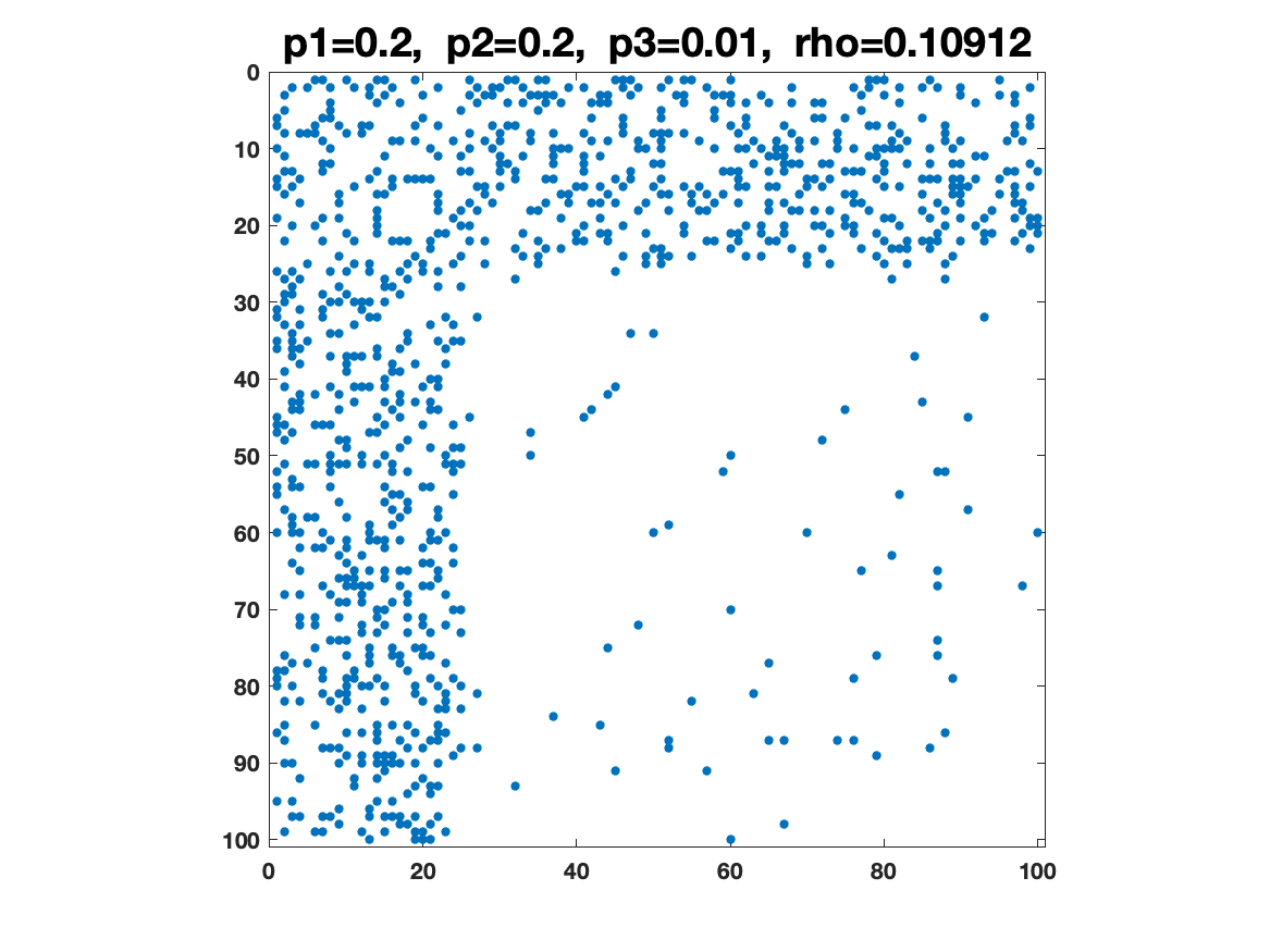
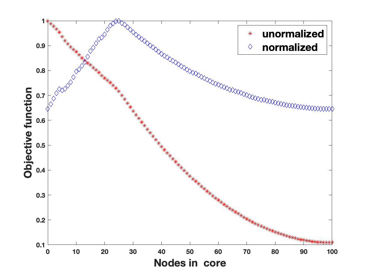
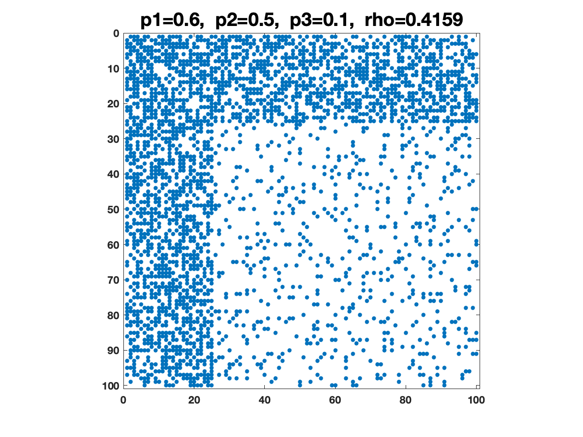
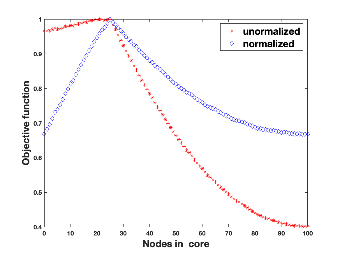
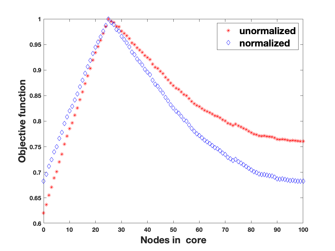
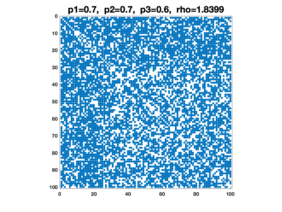
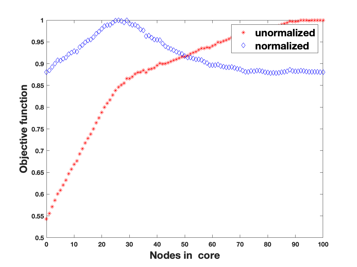
Figure 1: Left: Adjacency matrices with $M=25$ planted core nodes. Right: behaviour of the objective function (2) (red stars) and (3) (blue diamonds) as nodes are added into the core, using the original ordering. Each curve is scaled to have maximum value equal to one. The value of $\rho$ in (4) changes from $\approx 0.1$, to $0.4$, $1.2$ and $1.8$ as we move down the rows. The normalized objective function (3) peaks at the correct core size of 25 in each case.

We now alter the probability parameters. In the second level of Figure 1 the ratio of existing to missing edges is slightly more balanced; we have a sample from $\mathrm{SBM}(100,25,0.6,0.5,0.1)$, for which $\rho\approx 0.4$. We see that both measures now give a peak at core size 25, but the normalized version (3) gives a more pronounced result. The third level uses a sample from $\mathrm{SBM}(100,25,0.8,0.8,0.35)$. Here, $\rho\approx 1.2$, so the ratio is well balanced. Both measures are seen to perform effectively. At the opposite extreme to the first level, in the fourth level of Figure 1 we have the case of a dense network; here we sampled from $\mathrm{SBM}(100,25,0.7,0.7,0.6)$, with $\rho\approx 1.8$. We see that the unnormalized measure (2) favours the assignment of all nodes to the core, so that edges are predicted for every pair of nodes. The normalized version (3) continues to highlight the “correct” assignment of the first 25 nodes to the core, even though the structure is barely perceptible in the adjacency matrix plot.

In summary, we see that the normalization in (3) produces a measure that is insensitive to the edge density. This property is highly desirable in practice, since networks are typically sparse. Hence, we will focus on this objective function.

3.3 Quadratic Form

Because summing over $1$ and summing over $a_{ij}$ in (3) is not affected by the choice of $x$, maximizing (3) is equivalent to maximize

$$\sum_{i=1}^{N}\sum_{j=1,j\neq i}^{N}\left(a_{ij}(\frac{1}{N_{1}}+\frac{1}{N_{2}})-\frac{1}{N_{2}}\right)\max\{x_{i},x_{j}\}.$$

Rescaling by $N_{1}$ and using (4), we arrive at

$$\sum_{i=1}^{N}\sum_{j=1,j\neq i}^{N}\left(a_{ij}(1+\rho)-\rho\right)\max\{x_{i},x_{j}\}.$$ (5)

This expression has a direct interpretation: for every connected pair of nodes $i$ and $j$, where $a_{ij}=1$, we gain by $+1$ if the partition correctly predicts an edge ($\max\{x_{i},x_{j}\}=1$) and by zero otherwise. Similarly, for every disconnected pair of nodes $i$ and $j$, where $a_{ij}=0$, we lose out by $-\rho$ if the partition incorrectly predicts an edge ($\max\{x_{i},x_{j}\}=1$) and by zero otherwise.

Since $x$ has binary components, we have $\max\{x_{i},x_{j}\}=x_{i}+x_{j}-x_{i}x_{j}=x_{i}^{2}+x_{j}^{2}-x_{i}x_{j}$, and hence may write the objective function in (5) as

$$\sum_{i=1}^{N}\sum_{j=1,j\neq i}^{N}\left(a_{ij}(1+\rho)-\rho\right)(x_{i}^{2}+x_{j}^{2}-x_{i}x_{j}).$$ (6)

To find an appropriate QUBO formulation, we may expand (6) as

$$\sum_{i=1}^{N}x_{i}^{2}\sum_{j=1,j\neq i}^{N}\left(a_{ij}(1+\rho)-\rho\right)+\sum_{j=1}^{N}x_{j}^{2}\sum_{i=1,j\neq i}^{N}\left(a_{ij}(1+\rho)-\rho\right)-\sum_{i=1}^{N}\sum_{j=1,j\neq i}^{N}\left(a_{ij}(1+\rho)-\rho\right)x_{i}x_{j}.$$

Because $A$ is symmetric, the first two terms are equal, and we may rewrite the expression as

$$2\sum_{i=1}^{N}x_{i}^{2}\left(\mathrm{deg}_{i}(1+\rho)-(N-1)\rho\right)-\sum_{i=1}^{N}\sum_{j=1,j\neq i}^{N}\left(a_{ij}(1+\rho)-\rho\right)x_{i}x_{j}.$$

It follows that the maximization of (6) may be written in QUBO form:

$$\max_{x_{i}\in\{0,1\}}x^{T}Qx,\quad\text{~{}where~{}~{}~{}}Q=2(1+\rho)D-2(N-1)\rho I-A(1+\rho)+\rho E.\quad$$ (7)

We note in passing that the coefficient matrix defining a QUBO is not uniquely determined; for example, in any QUBO we can force $Q$ to be symmetric, upper triangular or lower triangular [18].

3.4 Modified QUBO Form

The D-Wave quantum annealer mentioned in section 4 can handle larger problem dimensions $N$ in (7) if the matrix $Q$ is sparse. We will assume now that the underlying network represented by the adjacency matrix $A$ is sparse, which also implies that the ratio $\rho$ in (4) is small. In this case the first three terms in the definition of $Q$ in (7) are sparse, and indeed on removing the final term, $\rho E$, the resulting matrix

$$\widehat{Q}=2(1+\rho)D-2(N-1)\rho I-A(1+\rho),$$ (8)

has the same sparsity as $A$.

Letting $x_{\mathrm{sum}}:=\sum_{i=1}^{N}x_{i}$, for any binary-valued $x$ we have

$$x^{T}Ex=x^{T}\left(\mathbf{1}\mathbf{1}^{T}-I\right)x=(x^{T}\mathbf{1})^{2}-x^{T}x=x_{\mathrm{sum}}^{2}-x_{\mathrm{sum}}.$$

Hence, we have

$$x^{T}Qx-x^{T}\widehat{Q}x=\rho\,x_{\mathrm{sum}}(x_{\mathrm{sum}}-1).$$ (9)

At an optimal value of $x$; that is, a binary vector maximizing (7), the quantity $x_{\mathrm{sum}}$ represents the number of nodes assigned to the core. For a sparse network we expect the core size to be small compared with $N$. Hence, the difference in (9) should be small relative to $x^{T}Qx$. So the original QUBO (7), which has a full matrix $Q$, should be well approximated by the sparse QUBO

$$\max_{x_{i}\in\{0,1\}}x^{T}\widehat{Q}x.$$ (10)

Based on this motivation, for large sparse networks where the original QUBO (7) cannot be treated by D-Wave, we will use the nearby sparse QUBO (10). However, for consistency we will judge the quality of the solution in terms of the original quadratic form $x^{T}Qx$ as in (7).

4 Quantum Annealing

Quantum annealers may only be applied to problems in QUBO form (or an equivalent Ising form). Although this restricts their practical usage, we note that many tasks arising in graph theory, scheduling and theoretical computer science may be expressed as QUBOs; see [8, 6] for recent examples and [18, 23] for comprehensive reviews.

The essence of quantum annealing is to move adiabatically from a “simple” Hamiltonian to a Hamiltonian that encodes the problem of interest. This annealing process makes use of quantum phenomena, including superposition and tunneling, to explore the solution landscape.

As discussed in [24], because quantum annealing takes place in a physical system it is subject to ambient noise and liable to suffer further imprecision resulting from the analog controls. For these reasons it is difficult to make general statements about either the theoretical computational complexity or the practical performance of a quantum annealer. However, there are indications [9] that quantum annealing, and quantum computing in general [1], have the potential to make a larger range of problems computationally feasible. Our approach in this work is to focus on the quality of solution provided by the quantum annealer and to compare this with the results obtained by existing heuristic approaches on a classical machine.

Our quantum annealing experiments are conducted on the Advantage 4.1 system from D-Wave [25], which is commercially available via remote access. The output is probabilistic, and hence it is common to request multiple samples for comparison. In our computations, we found that 100 samples was sufficient to provide consistent results. By default we will report on the best sample obtained.

For illustration, on the left in Figure 2 we show the adjacency matrix for a network used in [4, Table 4] concerning co-citations among social work journals. Here, the horizontal and vertical lines illustrate the partition proposed in [4] using a genetic algorithm to maximize the correlation between the data and an ideal pattern matrix. We see that five nodes have been placed in the core. In this case, the quantum annealer applied to the corresponding QUBO (7) produced the same core-periphery partitioning, thereby supporting the empirical result in [4]. For this partition, with $Q$ defined in (7), the objective function has the value $x^{T}Qx\approx 68.5$. For information, on the right in Figure 2 we also report the second-best partition returned by the quantum annealer; here an extra node (the original node $16$) has been placed in the core and the objective function value is $x^{T}Qx\approx 67.5$.

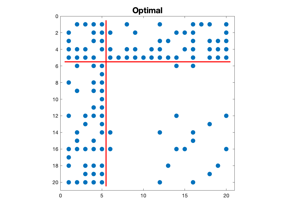
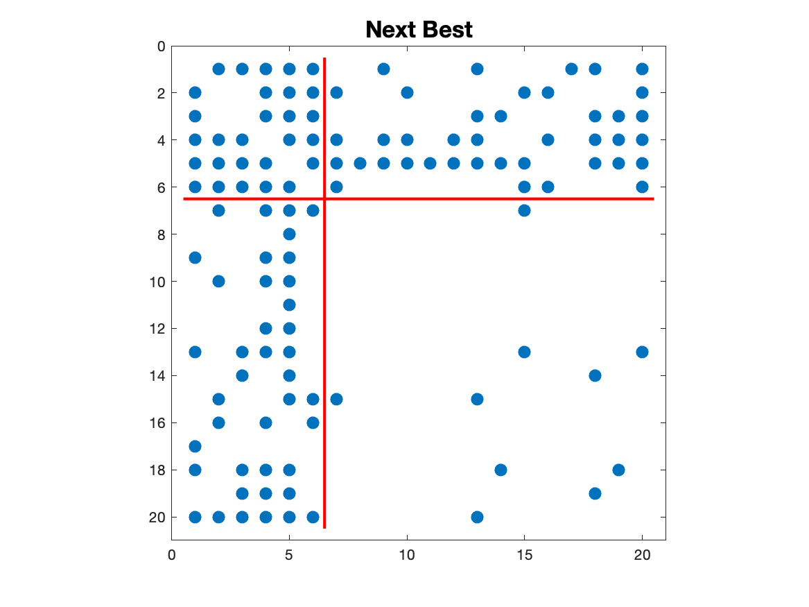
Figure 2: Left: Adjacency matrix with core-periphery partition from [4]. Right: second best core-periphery partition from the quantum annealer added an extra node to the core.

As a further illustration, in Figure 3 the nodes represent the 60 most commonly occurring adjectives and the 60 most commonly occurring nouns in the novel “David Copperfield” by Charles Dickens, and edges connect pairs of words that occur in adjacent positions in the text. (Eight nodes are disconnected from the rest of the network, and hence are ignored.) This network data, with 425 edges, comes from [26]. The picture on the left shows the adjacency matrix in the original ordering, and on the right we give the best core-periphery partition found by the quantum annealer. Further results for this network appear in Table 3 of section 5.

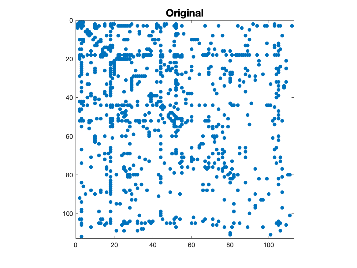
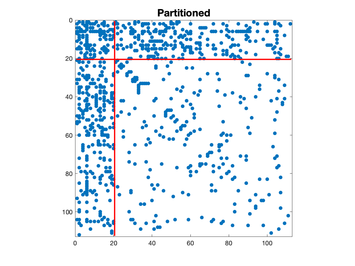
Figure 3: Left: Adjacency matrix from [26] with original node ordering. Right: best core-periphery partition from the quantum annealer.

5 Method Comparison

In this section we give quantitative results based on the new objective function (5), via the quadratic form in (7), as a means to compare various approaches to core-periphery partitioning.

5.1 Synthetic Data

We begin with two tests on stochastic block models that have some level of planted core-periphery structure. In Figure 4 we show samples from $\mathrm{SBM}(100,25,p_{1},p_{2},p_{3})$ with $p_{1}=p_{2}=p$ and $p_{3}=0.01$, for $p=0.1$, $p=0.08$, $p=0.06$ and $p=0.04$. Table 1 records the results. Here, each partitioning method produces a binary vector, $x\in\mathbb{R}^{100}$, and we show the corresponding value of $x^{T}Qx$ for $Q$ in (7). In parentheses we show the associated core size, $x_{\mathrm{sum}}$. For reach network, the two largest values of $x^{T}Qx$ are highlighted, with the largest value shown in bold. The first row, marked “Original”, shows the value of $x^{T}Qx$ arising when $x$ is taken to be the “correct” core set arising from the model; that is, $x_{i}=1$ for $1\leq i\leq 25$ and $x_{i}=0$ otherwise. We emphasize that due to the stochasticity this partitioning is not guaranteed to be optimal for a particular SBM sample; indeed, we see from the table that better choices exist in each case. The second and third rows, marked “$Q$” and “$\widehat{Q}$”, show results for the D-Wave solution to the QUBO (7) and (10), respectively. Rows four to nine correspond to techniques originally designed to output a vector of nonnegative values to be regarded as a measure of coreness. From these vectors, we find a binary partitioning vector $x$ by optimally thresholding the coreness vector: we assign value $x_{i}=1$ to the top $k$ nodes in terms of coreness, and $x_{i}=0$ to the remaining nodes, and then select the binary $x$ which attains the largest value of $x^{T}Qx$ over $0\leq k\leq N$. The corresponding $k$ is then taken to be the predicted core size. The fourth row, “Degree,” uses the degree vector $\mathrm{deg}_{i}$ as a measure of coreness. Similarly, the fifth, sixth and seventh rows, “EigA,” “EigQ” and “NonlinPM” use optimal partitions based on the coreness measures given by the Perron-Frobenius eigenvector of $A$, the dominant eigenvector of $Q$, and the corresponding nonlinear eigenvector from [30] (with parameter values $\alpha=10$ and $p=2\alpha$ taken from that work). We note that the use of the degree vector and the Perron-Frobenius vector of $A$ was suggested in [4] and has subsequently been studied by several authors; see for example, [28, 30, 32]. The “EigQ” method is motivated by the idea of using an eigenvector that solves a relaxed version of the QUBO (7), where $x\in\mathbb{R}^{N}$ is constrained to have $\|x\|_{2}=1$. The eighth row “$h$-index” uses the $k$-core decomposition coreness score [21], computed as the limit of the $h$-index operator sequence [22], while the ninth row “GenBE” corresponds to the generalization of the original Borgatti and Everett core measure [4] proposed in [28], where the quadratic form $x^{T}Ax$ is approximately maximimzed over a set of not-necessarily-binary core-periphery transition vectors $x$.

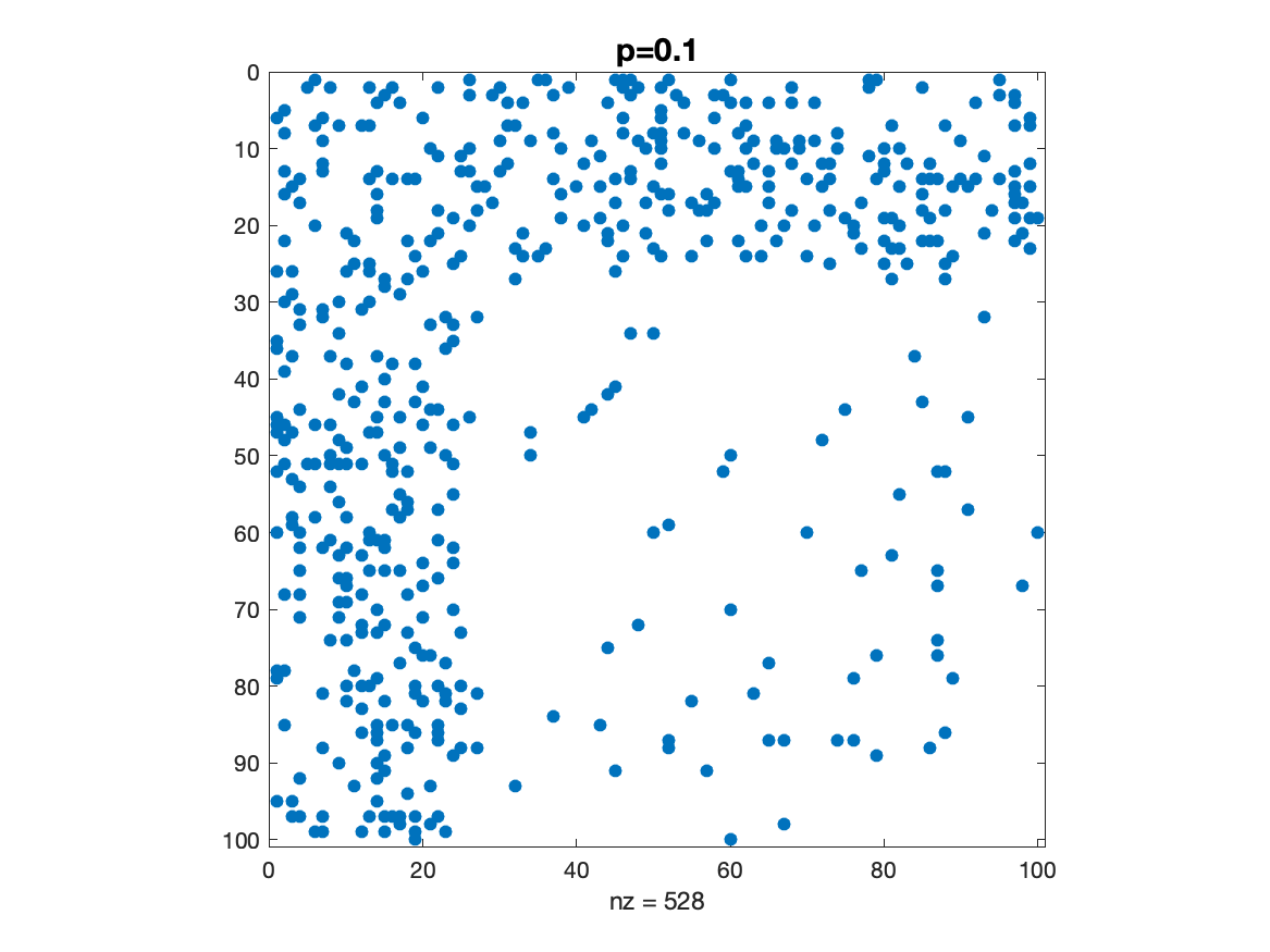
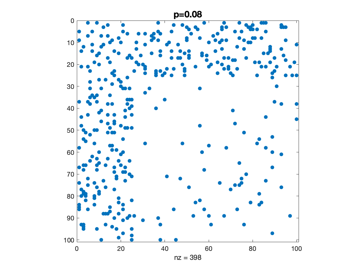
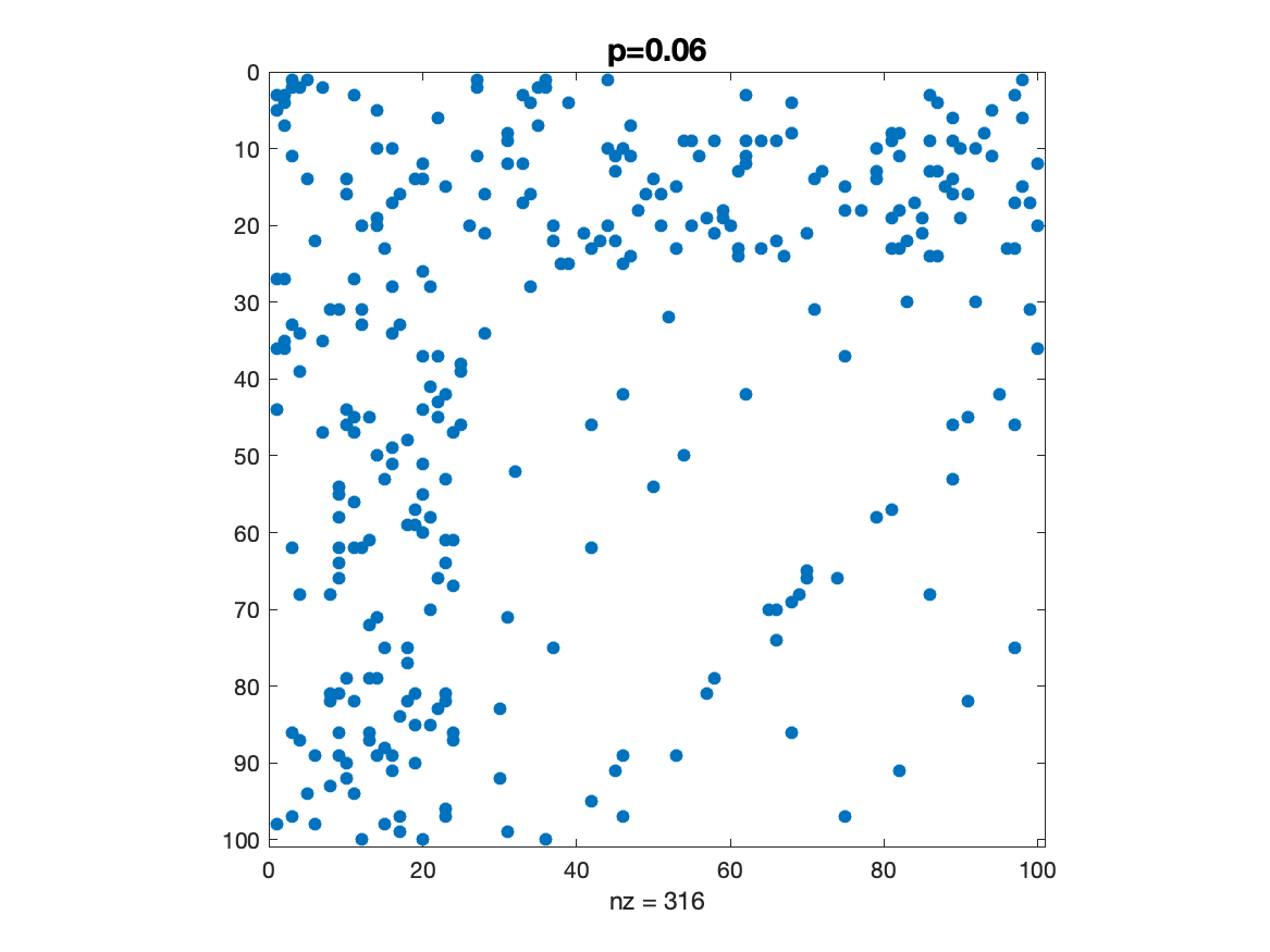
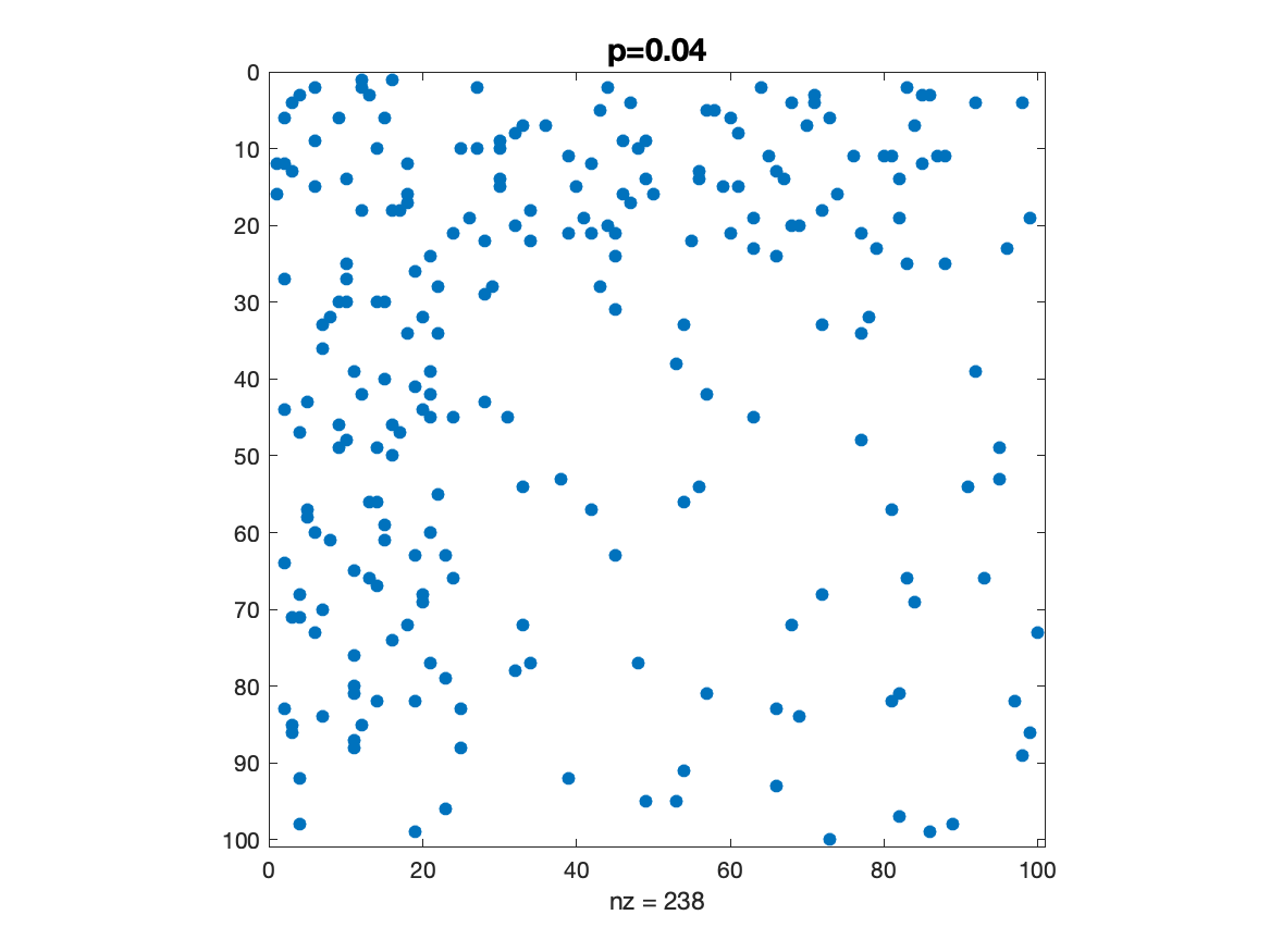
Figure 4: Small synthetic data: samples from $\mathrm{SBM}(100,25,p,p,0.01)$ for $p=0.1$, $p=0.08$, $p=0.06$ and $p=0.04$.

	$p=0.1$	$p=0.08$	$p=0.06$	$p=0.04$
Original	245.1 (25)	165.8 (25)	131.3 (25)	83.4 (25)
$Q$	255.7 (23)	174.5 (28)	183.4 (24)	101.3 (28)
$\widehat{Q}$	252.1 (21)	174.2 (24)	183.1 (22)	98.8 (22)
Degree	241.0 (26)	164.1 (28)	136.3 (24)	89.2 (24)
EigA	177.6 (23)	89.7 (20)	88.6 (27)	49.5 (27)
EigQ	119.0 (21)	86.6 (321)	59.0 (25)	70.0 (33)
NonlinPM	255.7 (23)	172.4 (28)	136.8 (26)	100.5 (30)
$h$-index	235.2 (21)	165.8 (25)	118.6 (19)	81.0 (24)
GenBE	150.3 (31)	91.4 (21)	90.0 (25)	56.0 (23)

Table 1: Values of the objective function value $x^{T}Qx$ from (7) for the $\mathrm{SBM}(100,25,p,p,0.01)$ samples shown in Figure 4, with core size in parentheses. Original: assigning the first $M=25$ nodes to the core; $Q$: quantum annealing on (7); $\widehat{Q}$: quantum annealing on (10); Degree: the nodal degrees; EigA: the eigenvector associated with dominate eigenvalue of the adjacency matrix $A$; EigQ: the eigenvector associated with dominate eigenvalue of the QUBO matrix $Q$; NonlinPM: the power method from [30] to compute a nonlinear eigenvector; $h$-index: the $k$-core decomposition coreness score from [21]; GenBE: the method from [28]. For reach network, the two largest values of $x^{T}Qx$ are highlighted, with the largest value shown in bold.

We see in Table 1 that, on these tests, the largest or joint-largest value of $x^{T}Qx$ is achieved by applying the quantum annealing algorithm directly to the QUBO (7). We also note that $Q$, $\widehat{Q}$ and NonlinPM improve on the $x^{T}Qx$ value provided by the planted “ground truth” from the original model. The two standard eigenvalue approaches are consistently the poorest in this measure.

In Figure 5 we show larger networks: these are samples from $\mathrm{SBM}(500,50,p,p,0.005)$ with $p=0.04$, $p=0.03$, $p=0.02$ and $p=0.01$. Here, the full QUBO (7) was too large for the quantum annealer. In Table 2 we show results for the remaining partioning methods. We see that quantum annealing with $\widehat{Q}$ gives the best result on three of the four cases, with NonlinPM also performing well.

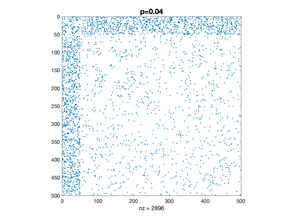
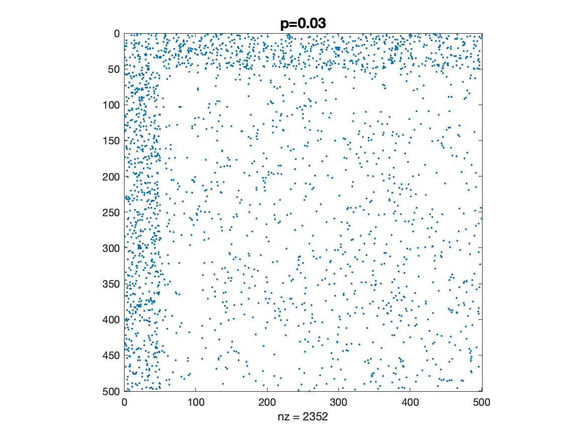
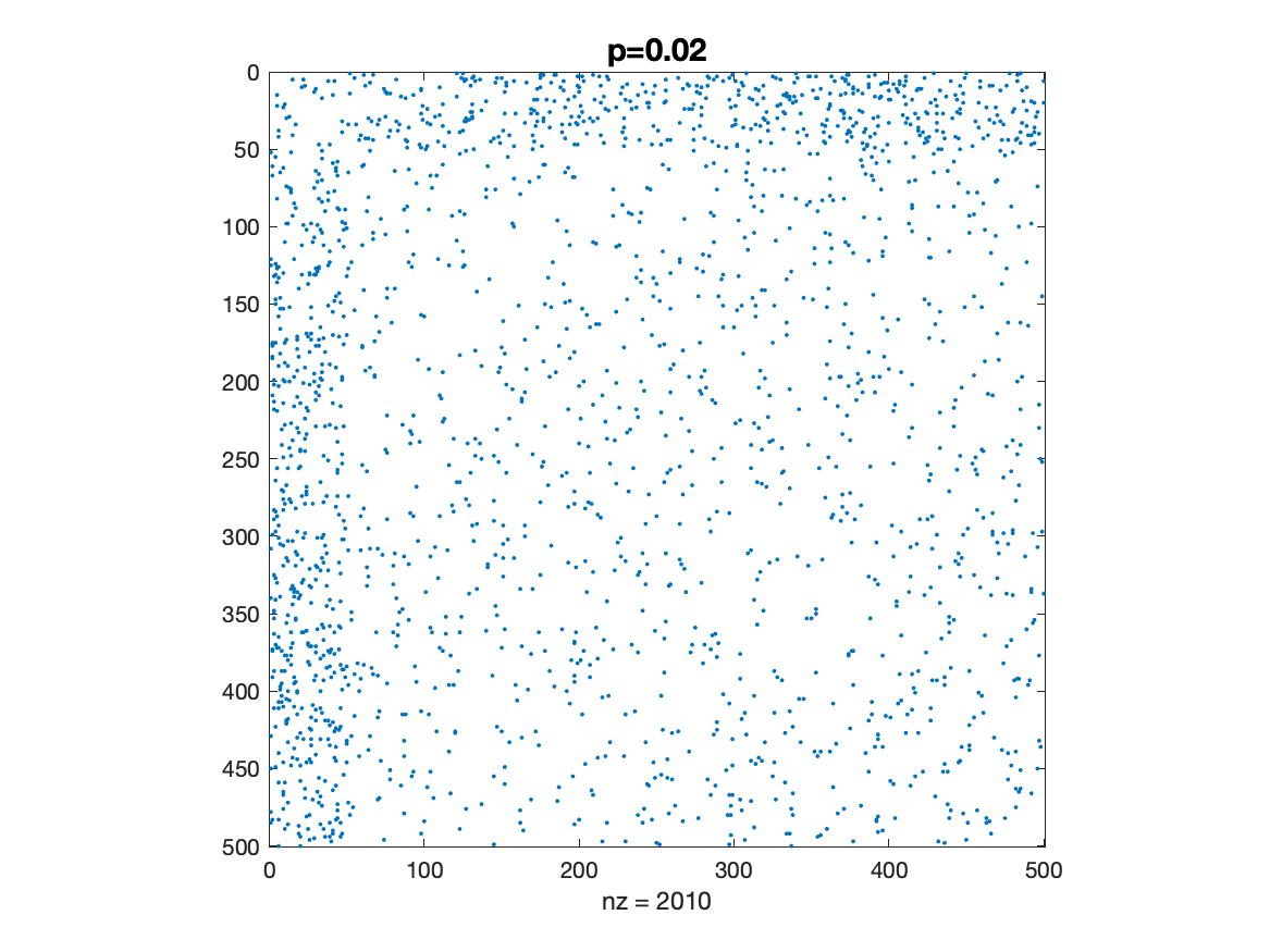
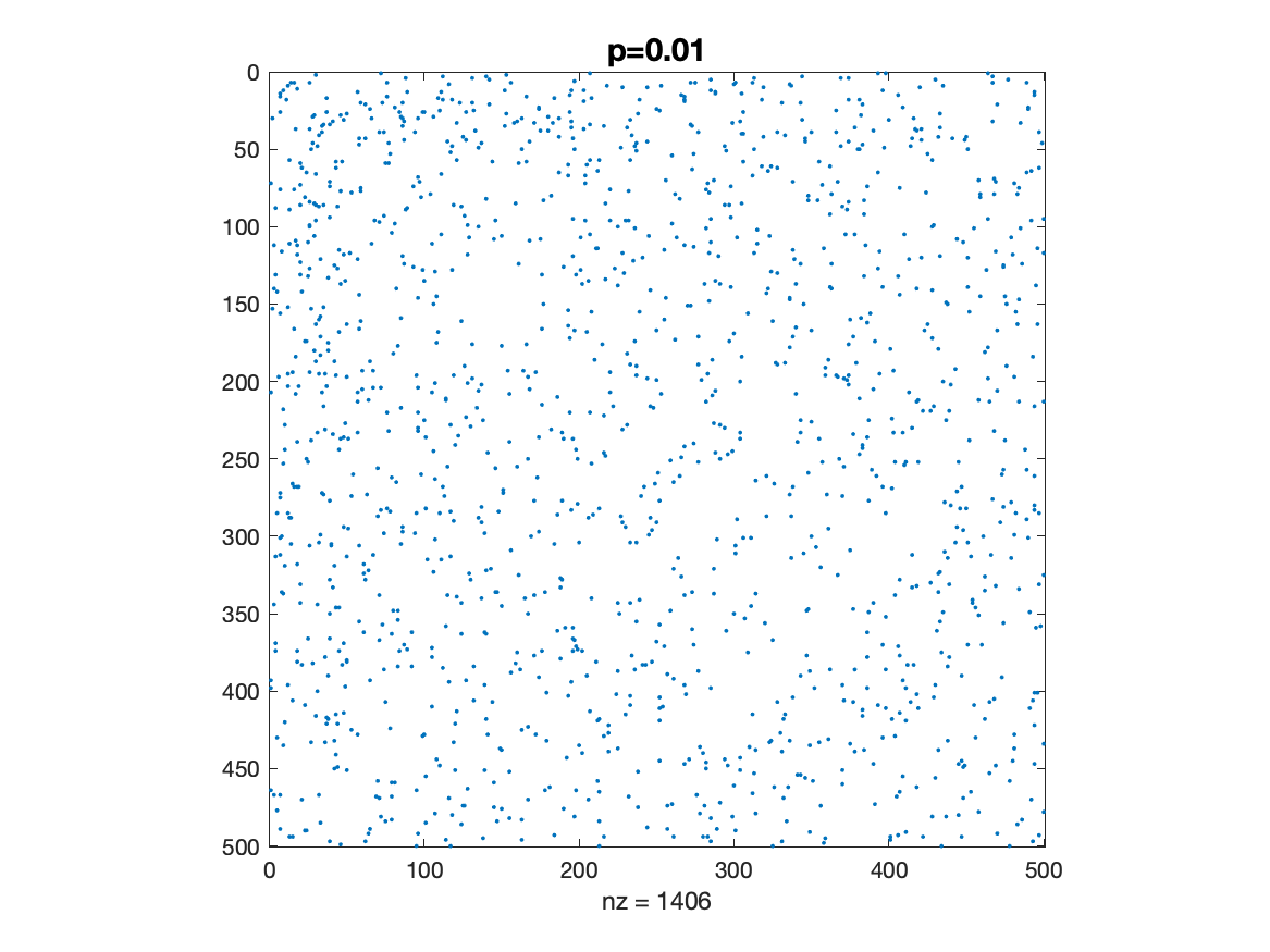
Figure 5: Larger synthetic data: samples from $\mathrm{SBM}(500,50,p,p,0.005)$ for $p=0.04$, $p=0.03$, $p=0.02$ and $p=0.01$.

	$p=0.04$	$p=0.03$	$p=0.02$	$p=0.01$
Original	1334.7 (50)	939.6 (50)	600.6 (50)	155.5 (50)
$\widehat{Q}$	1365.5 (62)	996.2 (72)	730.0 (88)	472.3 (120)
Degree	1350.7 (56)	970.4 (68)	670.3 (102)	368.7 (94)
EigA	1213.3 (66)	726.9 (87)	431.2 (75)	189.9 (84)
EigQ	768.8 (111)	428.9 (111)	219.8 (196)	362.3 (198)
NonlinPM	1363.1 (72)	1002.2 (90)	729.2 (101)	465.7 (157)
$h$-index	1334.7 (50)	920.4 (48)	605.4 (51)	206.0 (116)
GenBE	1320.1 (57)	915.4 (76)	554.7 (99)	290.0 (151)

Table 2: As in Table 1 for the $\mathrm{SBM}(500,50,p,p,0.005)$ samples shown in Figure 5. Here the networks are too large for quantum annealing on the full QUBO (7).

5.2 Real Data

Table 3 shows results for the following real networks:

USAir97

is from [12], with weights binarized. The $N=332$ nodes represent airports in USA. The 2126 undirected edges indicate whether at least one scheduled USAir flight took place between the two airports in 1997.

Celegans

has 277 nodes and 2105 edges that represent neurons and synapses in the worm Caenorhabditis elegans. The data is from https://www.cs.cornell.edu/~arb/data/ based on [17].

Jazz

from [7] is a network of 198 jazz bands (nodes) that performed between 1912 and 1940, and 2742 corresponding edges (musicians).

Adjnoun

was described in section 4.

Football

from [16], is a network of American football games between 115 Division IA colleges during the fall 2000 regular season. Here, nodes represent teams and the 613 edges represent fixtures.

Journals

from [2], has 5972 edges representing shared interests among 124 magazines and journals, which form the nodes, based on a sample of $\sim 100,000$ residents of Ljubljana (Slovenia) in survey conducted in 1999 and 2000.

	USAir97	Celegans	Jazz	Adjnoun	Football	Journals
$Q$	x	x	x	352.5 (20)	93.8 (51)	7360.5 (54)
$\widehat{Q}$	2703.7 (38)	1620.3 (42)	1743.1 (39)	351.8 (18)	33.6 (12)	4091.6 (23)
Degree	2677.1 (35)	1601.7 (49)	1772.6 (51)	345.1 (23)	27.9 (38)	7360.5 (54)
EigA	2598.3 (37)	1243.8 (21)	1400.6 (37)	314.5 (19)	6.4 (4)	7355.2 (52)
EigQ	310.7 (5)	1414.2 (40)	541.6 (16)	158.2 (13)	77.5 (54)	3741.1 (23)
NonlinPM	2699.5 (38)	501.4 (28)	1792.4 (47)	345.3 (22)	76.4 (38)	7358.8 (53)
$h$-index	2534.9 (42)	258.8 (18)	884.4 (60)	242.7 (32)	14.1 (89)	4156.1 (39)
GenBE	2626.1 (34)	815.8 (35)	1364.3 (30)	298.4 (21)	3.9 (2)	7349.6 (53)

Table 3: As in Table 1 for the real networks described in the text. The symbol “x” denotes that the problem (7) was too large for the quantum annealer.

We see that on the three smaller networks in Table 3, quantum annealing with $Q$ produced the best or joint-best results. The x symbol indicates that the first three problems produced a QUBO (7) that was too large for the quantum annealer. Two of the top results on the three larger networks are produced by quantum annealing with $\widehat{Q}$ and the nonlinear power method is best on the third. So, overall, a quantum annealing approach is best or joint-best on five out of the six networks.

6 Discussion

We have shown that the new objective function (3) gives a straightforward, parameter-free, method for (a) judging a core-periphery partition and also (b) determining a partition from a real-valued vector of scores. Moreover, when written in QUBO form the resulting discrete maximization problem is amenable to quantum annealing. We found that the D-Wave quantum annealer could handle QUBOs of this form for networks with $\approx 100$ nodes. In principle a quantum annealer is able to find a globally optimum solution. In practice, of course, as with any physical system various sources of noise can affect the performance. However, we observed that direct application of the quantum annealer always produced the best or joint-best result in comparison with current heuristic core-periphery detection algorithms. Moreover, a sparsified version of the QUBO allowed the quantum annealer to be applied on networks of size $N=500$ and also gave good results.

Given the likely future performance advancements and increased take-up of this technology, our work suggests that a QUBO/quantum annealing approach has great promise in this application area.

We also emphasize that the quantum annealer typically delivers multiple “samples” that correspond to approximate solutions of the QUBO. We focused here on the quality of the best sample out of 100; that is, the binary sample $x$ for which the quadratic form in (7) was maximum. However, we observed that the full set of samples typically included many different almost-optimal alternatives. Hence the quantum annealer could also be used to produce coreness scores or rankings across the nodes by, for example, counting the frequency with which each node was assigned to the core.

We saw in our experiments that the classical (linear) eigenvector methods did not perform well in terms of providing approximate solutions to the QUBO (7). Intuitively, these types of spectral approaches are closely tied with smooth, least-squares type kernels [19, 31], and hence the relaxed optimization problems that they solve are significantly different from (1). The GenBE method from [28] aims at maximizing the same type of quadratic spectral kernel, but constrained to a smaller set of indicator-type vectors. While doing better than the purely-quadratic methods, it still did not perform well in our context. The $h$-index method from [21] also performed poorly in these tests—the $k$-core construction is likely to be more useful when the core-periphery interactions are less plentiful. The nonlinear power method from [30] was more successful. This method directly approximates the maximum in (1) before relaxing to a real-valued problem and adding a constraint. More precisely, for $y,z\in\mathbb{R}$ and $\alpha>1$, consider the softmax function

$$\mu_{\alpha}(y,z)=\left(|y|^{\alpha}+|z|^{\alpha}\right)^{1/\alpha}.$$ (11)

Also define the $p$-sphere ${\cal S}_{p}=\{x\in\mathbb{R}^{N}:\|x\|_{p}=1\}$ and let ${\cal S}_{p}^{+}={\cal S}_{p}\cap\mathbb{R}^{N}_{+}$. Then the method in [30] gives a globally convergent iteration for the unique solution of

$$\max_{x\in{\cal S}_{p}^{+}}\sum_{i=1}^{N}\sum_{j=1}^{N}a_{ij}\mu_{\alpha}(x_{i},x_{j}).$$

Note that for large $\alpha$ the function $\mu_{\alpha}(y,z)$ in (11) is a good approximation to $\max\{y,z\}$. Based on our results, it would therefore be of interest to design and analyse a similar nonlinear power method that applies to the new objective function (3) rather than the original version (1).

References

- [1] F. Arute et al. Quantum supremacy using a programmable superconducting processor. Nature, 574:505–510, 2019.
- [2] V. Batagelj and A. Mrvar. Pajek datasets. http://vlado.fmf.uni-lj.si/pub/networks/data/, 2006.
- [3] A. R. Benson and J. Kleinberg. Found graph data and planted vertex covers. In S. Bengio, H. Wallach, H. Larochelle, K. Grauman, N. Cesa-Bianchi, and R. Garnett, editors, Advances in Neural Information Processing Systems, volume 31. Curran Associates, Inc., 2018.
- [4] S. P. Borgatti and M. G. Everett. Models of core/periphery structures. Social Networks, 21:375–395, 2000.
- [5] M. Brusco. An exact algorithm for a core/periphery bipartitioning problem. Social Networks, 33(1):12–19, 2011.
- [6] G. Chapuis, H. N. Djidjev, G. Hahn, and G. Rizk. Finding maximum cliques on the D-Wave quantum annealer. J. Signal Process. Syst., 91(3-4):363–377, 2019.
- [7] Y. Choe, B. McCormick, and W. Koh. Network connectivity analysis on the temporally augmented c. elegans web: A pilot study. 30(921.9), 2004.
- [8] E. Cocchi, E. Tignone, and D. Vodola. Graph partitioning into Hamiltonian subgraphs on a quantum annealer. arXiv:2104.09503, 2021.
- [9] E. Crosson and D. Lidar. Prospects for quantum enhancement with diabatic quantum annealing. Nat. Rev. Phys., 3:466–489, 2021.
- [10] P. Csermely, A. London, L.-Y. Wu, and B. Uzzi. Structure and dynamics of core/periphery networks. Journal of Complex Networks, 1(2):93–123, 2013.
- [11] M. Cucuringu, P. Rombach, S. H. Lee, and M. A. Porter. Detection of core–periphery structure in networks using spectral methods and geodesic paths. European Journal of Applied Mathematics, 27(6):846–887, 2016.
- [12] T. A. Davis and Y. Hu. The University of Florida sparse matrix collection. ACM Transactions on Mathematical Software, 38:1–25, 2011.
- [13] E. Estrada and P. A. Knight. A First Course in Network Theory. Oxford University Press, 2015.
- [14] D. Fasino and F. Rinaldi. A fast and exact greedy algorithm for the core–periphery problem. Symmetry, 12(1), 2020.
- [15] R. J. Gallagher, J.-G. Young, and B. F. Welles. A clarified typology of core-periphery structure in networks. Science Advances, 7(12):eabc9800, 2021.
- [16] M. Girvan and M. E. Newman. Community structure in social and biological networks. Proceedings of the National Academy of Sciences, 99(12):7821–7826, 2002.
- [17] P. Gleiser and L. Danon. Community structure in jazz. Advances in Complex Systems, 6:565–573, 2003.
- [18] F. W. Glover, G. A. Kochenberger, and Y. Du. Quantum bridge analytics I: a tutorial on formulating and using QUBO models. 4OR, 17(4):335–371, 2019.
- [19] D. J. Higham, G. Kalna, and M. J. Kibble. Spectral clustering and its use in bioinformatics. J. Computational and Applied Math., 204:25–37, 2007.
- [20] P. Holme. Core-periphery organization of complex networks. Physical Review E, 72(4):046111, 2005.
- [21] M. Kitsak, L. K. Gallos, S. Havlin, F. Liljeros, L. Muchnik, H. E. Stanley, and H. A. Makse. Identification of influential spreaders in complex networks. Nature Physics, 6(11):888, 2010.
- [22] L. Lü, T. Zhou, Q.-M. Zhang, and H. E. Stanley. The H-index of a network node and its relation to degree and coreness. Nature Communications, 7:10168, 2016.
- [23] A. Lucas. Ising formulations of many NP problems. Frontiers in Physics, 2:1–16, 2014.
- [24] C. C. McGeoch. Theory versus practice in annealing-based quantum computing. Theoretical Computer Science, 816:169–183, 2020.
- [25] C. C. McGeoch and P. Farré. The Advantage system: Performance update. Technical Report 14-1054A-A, D-Wave Systems Inc., Burnaby, Canada, 2021.
- [26] M. E. J. Newman. Finding community structure in networks using the eigenvectors of matrices. Phys. Rev. E, 74:036104, Sep 2006.
- [27] M. Papachristou. Sublinear domination and core-periphery networks. Scientific Reports, 11, 2021.
- [28] M. P. Rombach, M. A. Porter, J. H. Fowler, and P. J. Mucha. Core-periphery structure in networks (revisited). SIAM Review, 59:619–646, 2017.
- [29] F. Tudisco, A. R. Benson, and K. Prokopchik. Nonlinear higher-order label spreading. In Proceedings of the Web Conference, 2021.
- [30] F. Tudisco and D. J. Higham. A nonlinear spectral method for core-periphery detection in networks. SIAM J. Mathematics of Data Science, 1:269–292, 2019.
- [31] U. von Luxburg. A tutorial on spectral clustering. Statistics and Computing, 17(4):395 – 416, 2007.
- [32] X. Zhang, T. Martin, and M. E. J. Newman. Identification of core-periphery structure in networks. Phys. Rev. E, 91:032803, 2015.