Two-loop mixed QCD-EW corrections to neutral current Drell-Yan

Abstract

We present the two-loop mixed strong-electroweak virtual corrections to the neutral current Drell-Yan process and we provide, in ancillary files, the explicit formulae of the infrared-subtracted finite remainder. The final state collinear singularities are regularised by the lepton mass. The evaluation of all the relevant Feynman integrals, including those with up to two internal massive lines, has been worked out relying on analytical and semi-analytical techniques, in the case of complex-valued masses.

1 Introduction

At hadron colliders, the production of a pair of leptons each with large transverse momentum, also known as Drell-Yan (DY) process Drell:1970wh , has played a central role in the development of the Standard Model (SM) of the strong and electroweak (EW) interactions. The same process that allowed the discovery of the $W$ and $Z$ bosons Arnison:1983rp ; Banner:1983jy ; Arnison:1983mk ; Bagnaia:1983zx provides today very precise information about the gauge sector of the SM and allows its test at the quantum level. The determination of the masses of the gauge bosons and of the effective weak mixing angle, with relative errors at the 0.01% and 0.1% level respectively Group:2012gb ; Aaboud:2017svj ; Aaltonen:2018dxj ; ATLAS:2018gqq , is possible thanks to the excellent quality of the data collected at the Fermilab Tevatron by the CDF and D0 experiments and at the CERN LHC by the ATLAS, CMS, and LHCb experiments. The kinematical distributions are fitted by using theoretical templates, keeping the EW parameters as fitting variables. The uncertainty in the evaluation of the templates enters in the total error of the experimental value as a theoretical systematic contribution CarloniCalame:2016ouw ; Bagnaschi:2019mzi ; Behring:2021adr . Hence, it is of utmost importance to minimise the latter in order to make the comparison more significant. The direct search for signals of New Physics is carried on, in the DY process, with the precise measurement of the tail of the kinematical distributions. A deviation could then be interpreted as the distortion due to a new resonance or, in general, as the effect of a new higher-dimensional operator whose increment with the energy shows up in the tails. In order to appreciate the possibility of such a deviation, the most precise SM prediction is needed, with the smallest possible residual theoretical uncertainty. The inclusion of higher-order corrections makes the theoretical predictions more precise, but it requires to overcome challenging mathematical and computational problems.

The radiative corrections to the DY processes in the strong coupling $\alpha_{s}$ were computed at next-to-leading-order (NLO) Altarelli:1979ub and next-to-next-to-leading-order (NNLO) Hamberg:1990np ; Harlander:2002wh in perturbative Quantum Chromodynamics (QCD). Recently, the calculations at next-to-next-to-next-to-leading-order (N³LO) QCD of the inclusive production of a virtual photon Duhr:2020seh , a $W$ boson Duhr:2020sdp , and for the total neutral current (NC) DY process Duhr:2021vwj have been completed. Fully differential NNLO QCD computations including the leptonic decay of the vector boson have been presented in refs. Anastasiou:2003yy ; Anastasiou:2003ds ; Melnikov:2006kv ; Catani:2009sm ; Catani:2010en , and the first estimates of the fiducial cross sections for the NC DY process at N³LO QCD have appeared Camarda:2021ict . A plethora of papers discusses the inclusion of higher-order corrections in the threshold region Moch:2005ky ; Laenen:2005uz ; Ravindran:2005vv ; Ravindran:2006cg ; deFlorian:2012za ; Ahmed:2014cla ; Catani:2014uta ; Li:2014afw ; Ajjath:2020ulr . The complete NLO EW corrections in the EW coupling $\alpha$ have been computed for $W$ production in refs. Dittmaier:2001ay ; Baur:2004ig ; Zykunov:2006yb ; Arbuzov:2005dd ; CarloniCalame:2006zq , while the $Z$ production case has been considered in refs. Baur:2001ze ; Zykunov:2005tc ; CarloniCalame:2007cd ; Arbuzov:2007db ; Dittmaier:2009cr . The NLO QCD and NLO EW corrections are separately large, often reaching the ${\cal O}(10-20\%)$ of the leading order (LO) when we consider differential kinematical distributions, raising the suspect that also mixed NNLO QCD-EW effects might be potentially large. The fact that in specific phase-space corners NLO QCD and NLO EW corrections have opposite signs leads to large cancellations Balossini:2009sa . When such cancellations take place, a reliable estimate of the residual uncertainties based on the previous orders is problematic, since in these regions we might expect non-negligible effects from the next perturbative orders. Only an explicit calculation can solve the problem.

The combination of NLO QCD and EW results, consistently matched with QCD and QED Parton Showers, has been presented in Bernaciak:2012hj ; Barze:2012tt ; Barze:2013fru ; Frederix:2018nkq . These Monte Carlo tools provide an approximation of the mixed QCD-EW corrections, valid in the soft and/or collinear limits for the radiation of multiple additional partons, but can not assess the size of the genuine NNLO QCD-EW terms. Instead, they provide a rough estimate of the residual uncertainties.

Since high precision is required by the studies aiming at the determination of the EW parameters and the searches for New Physics, an important effort of the theory community has been recently devoted to the evaluation of the mixed QCD-EW corrections. The NNLO mixed QCD-QED corrections were obtained in ref. deFlorian:2018wcj for the inclusive production of an on-shell $Z$ boson and extended at differential level for the decay of the $Z$ boson into a pair of neutrinos  Cieri:2020ikq . The production of an on-shell $Z$ boson, including NNLO mixed QCD-QED initial state corrections, but also the factorised NLO QCD corrections to $Z$ production and the NLO QED corrections to the leptonic $Z$ decay, has been discussed in ref. Delto:2019ewv . The complete NNLO QCD-EW corrections at ${\cal O}(\alpha\alpha_{s})\leavevmode\nobreak\$in analytical form for the total cross section production of an on-shell $Z$ bosons have been presented in refs. Bonciani:2016wya ; Bonciani:2019nuy ; Bonciani:2020tvf ; Bonciani:2021iis , whereas results differential in the final-state leptonic variables have been presented in refs. Buccioni:2020cfi and  Behring:2020cqi for the on-shell $Z$ and $W$ production respectively. Beyond the on-shell approximation, results have been obtained in the pole approximation Denner:2019vbn , which offers the possibility to move beyond the strictly on-shell limit and is based on a systematic expansion around the $W$ or $Z$ resonance. By definition, its range of validity is expected to be restricted to this phase-space region. The dominant part of the mixed QCD-EW corrections at the $W$ or $Z$ resonances has been evaluated with this technique in refs. Dittmaier:2014qza ; Dittmaier:2015rxo . Precise predictions at NNLO QCD-EW level in the whole phase-space have been obtained in ref. Dittmaier:2020vra for the subset of ${\cal O}(n_{F}\alpha_{s}\alpha)$. The charged-current DY process $pp\to\ell\nu_{\ell}+X$, has been considered in ref. Buonocore:2021rxx including the mixed QCD-EW corrections, with the reweighted two-loop virtual corrections in the pole approximation and all the other contributions in exact form. Very recently the complete set of NNLO QCD-EW corrections to the NC DY process $pp\to\ell^{+}\ell^{-}+X$ has been presented in ref. Bonciani:2021zzf , with the inclusion of the exact two-loop virtual contributions.

The virtual contributions were one of the bottlenecks for a complete ${\cal O}(\alpha_{s}\alpha)$ calculation, because the evaluation of the $2\to 2$ two-loop Feynman diagrams with internal masses is at the frontier of current computational techniques. Progress on the evaluation of the corresponding two-loop master integrals has been reported in refs. Bonciani:2016ypc ; Heller:2019gkq ; Hasan:2020vwn ; Long:2021fdc and, recently, the computation of the two-loop helicity amplitudes for NC massless lepton pair production was discussed in ref. Heller:2020owb . In this article, we provide in detail the independent computation at ${\cal O}(\alpha\alpha_{s})\leavevmode\nobreak\$of the two-loop amplitude for the process $q\bar{q}\to\ell^{+}\ell^{-}$. The calculation considers a massive leptonic final state, and features collinear logarithms of the lepton mass. These results, combined with the remaining perturbative contributions, allow the numerical evaluation of the hadron-level cross-section at this perturbative order, as presented in Bonciani:2021zzf .

In Section 2, we provide the framework of our computation, with the description of the treatment of $\gamma_{5}$ and of the ultraviolet (UV) renormalisation procedure. In Section 3, the details of the computation are presented, from the amplitude level until the renormalised matrix elements. In Section 4, the infrared (IR) subtraction procedure is discussed. In Section 5 we describe how we obtain the UV renormalised IR subtracted finite remainder and we present the details necessary for the numerical evaluation of the analytical expressions. In Section 6 we draw our conclusions. The unrenormalised matrix elements in terms of master integrals, together with a benchmark grid for the finite reminder, are provided as ancillary material. Appendix A gives the reader the information needed to make use of the files.

2 Framework of the Calculation

2.1 The process

We consider two-loop mixed QCD-EW corrections to lepton pair production in the quark annihilation channel, as given by

$$q(p_{1})+\bar{q}(p_{2})\rightarrow l^{-}(p_{3})+l^{+}(p_{4})\,.$$ (1)

We have separately computed the results for the $u\bar{u}$ and $d\bar{d}$ channels, with $u$ and $d$ denoting generic massless up- and down-type quarks. In the paper we present explicit results for the $u\bar{u}$ channel. The bare amplitude for this partonic process admits a double perturbative expansion in the two coupling constants

$$|\hat{\cal M}\rangle=|\hat{\cal M}^{(0)}\rangle+\left(\frac{\hat{\alpha}_{s}}{4\pi}\right)|\hat{\cal M}^{(1,0)}\rangle+\hat{\left(}\frac{\alpha}{4\pi}\right)|\hat{\cal M}^{(0,1)}\rangle+\left(\frac{\hat{\alpha}_{s}}{4\pi}\right)\hat{\left(}\frac{\alpha}{4\pi}\right)|\hat{\cal M}^{(1,1)}\rangle+\cdots$$ (2)

In this paper, we present the calculation of the following interference terms:

$$\langle\hat{\cal M}^{(0)}|\hat{\cal M}^{(1,0)}\rangle\,,\leavevmode\nobreak\ \leavevmode\nobreak\ \langle\hat{\cal M}^{(0)}|\hat{\cal M}^{(0,1)}\rangle\,,\leavevmode\nobreak\ \leavevmode\nobreak\ \langle\hat{\cal M}^{(0)}|\hat{\cal M}^{(1,1)}\rangle\,,$$ (3)

which contribute at ${\cal O}(\alpha\alpha_{s})\leavevmode\nobreak\$to the unpolarised squared matrix element of the process in eq. (1). These scalar quantities contain many one- and two-loop Feynman integrals. We apply the integration-by-parts (IBP) Tkachov:1981wb ; Chetyrkin:1981qh and Lorentz invariance (LI) Gehrmann:1999as identities to reduce those scalar Feynman integrals to a limited set, the so-called master integrals (MIs). The corrections in eq. (3) can then be expressed as the sum of the MIs, each multiplied by its corresponding coefficient. The latter are rational functions of the kinematical invariants and of the masses which appear in the process.

Virtual corrections are affected by singularities both of UV and IR type. The renormalisation procedure allows us to cancel the UV divergences and to express the amplitude in terms of renormalised parameters, which are in turn related to measurable quantities. The presence of IR divergences in the virtual corrections, on the other hand, is the counterpart of those which appear upon phase-space integration in the processes with the emission of additional massless partons, in our case a photon and/or a gluon. The universality of the IR divergent structure of the scattering amplitudes arising from soft and/or collinear radiation has been widely discussed in the literature and allows us to build a subtraction term, independently of the details of the full two-loop calculation. We exploit this property to check the consistency of our computation, in particular for the prescription related to the Dirac $\gamma_{5}$ matrix. To regularise both UV and IR divergences, we work in $d=4-2\varepsilon$ space-time dimensions. The renormalised amplitude can thus be written as a Laurent expansion in $\varepsilon$. At one-loop level we have:

$$\langle{\cal M}^{(0)}|{\cal M}^{(0,1)}\rangle\, = \sum_{i=-2}^{2}\varepsilon^{i}C^{(0,1)}_{i}(s,t,\mu_{\scriptscriptstyle W},\mu_{\scriptscriptstyle Z},m_{\ell})\,,$$ (4)

$$\langle{\cal M}^{(0)}|{\cal M}^{(1,0)}\rangle\, = \sum_{i=-2}^{2}\varepsilon^{i}C^{(1,0)}_{i}(s,t,\mu_{\scriptscriptstyle W},\mu_{\scriptscriptstyle Z},m_{\ell})\,,$$ (5)

while at two-loop we have:

$$\langle{\cal M}^{(0)}|{\cal M}^{(1,1)}\rangle\, = \sum_{i=-4}^{0}\varepsilon^{i}C^{(1,1)}_{i}(s,t,\mu_{\scriptscriptstyle W},\mu_{\scriptscriptstyle Z},m_{\ell})\,.$$ (6)

In eq. 6 we have retained only terms up to $\varepsilon^{0}$, as we are only interested in the finite cotributions at NNLO. However, this series contains higher powers of $\varepsilon$ which will be relevant for higher-order calculations. In these expressions $m_{l}$ is the lepton mass, and $\mu_{\scriptscriptstyle W}$, $\mu_{\scriptscriptstyle Z}$ are the complex masses of the $W$ and $Z$ boson defined as:

$$\mu_{V}^{2}=M_{V}^{2}-iM_{V}\Gamma_{V}\;.$$ (7)

The mass and decay width $M_{V},\Gamma_{V}$ are real parameters and are the pole quantities, i.e. correspond to the position of the pole in the complex plane of the gauge boson propagator. We also introduce the Mandelstam variables, defined as follows:

$$s=(p_{1}+p_{2})^{2},\,t=(p_{1}-p_{3})^{2},\,u=(p_{2}-p_{3})^{2}\,\,{\rm with}\,\,s+t+u=2m_{l}^{2}\,.$$ (8)

The on-shell conditions of the external particles are given by

$$p_{1}^{2}=p_{2}^{2}=0;\leavevmode\nobreak\ p_{3}^{2}=p_{4}^{2}=m_{l}^{2};$$ (9)

The coefficients $C_{i}$ in eq. (6) constitute the IR-unsubtracted two-loop interference terms, while those in eqs. (4,5), computed at one-loop, are necessary to prepare the subtraction term. The IR-subtracted expressions that can be obtained by their combination constitutes the main result that we present in this paper.

2.2 Treatment of $\gamma_{5}$ in Dimensional Regularisation

The calculation of radiative corrections, including chiral quantities in dimensional regularisation, faces the problem of defining a generalisation of the inherently four-dimensional object $\gamma_{5}$ in the arbitrary space-time dimension $d$. In 'tHooft:1972fi , ’t Hooft and Veltman proposed to abandon, in $d$ dimensions, the anticommutation relation of $\gamma_{5}$

$$\{\gamma_{\mu},\gamma_{5}\}=0$$ (10)

and to keep the cyclicity of the Dirac traces; the price is a significant computational load, due to the different treatment of the four-momenta components defined in the four space-time dimensions and of those in the remaining $d-4$. In refs. Kreimer:1989ke ; Korner:1991sx Kreimer et al. retained the anticommutation relation, with a substantial computational gain, and abandoned the cyclicity property of the trace operation. It was demonstrated that, at least in one-loop calculations, the choice of a unique point to start the evaluation of all the traces needed in one calculation leads to the systematic cancellation of the prescription dependent terms, along with that of the IR poles. It has recently been explicitly checked in ref. Heller:2020owb , for the NC DY process at ${\cal O}(\alpha\alpha_{s})\leavevmode\nobreak\$​, that the implementations at two-loop level of the ’t Hooft-Veltman-Breitenloner-Mason and of the Kreimer prescriptions yield, as expected, different results for the scattering amplitudes, but are in perfect agreement when one considers the finite correction after subtraction of all the IR divergences.

In this computation, we retain the anticommutation relation together with

$$\gamma_{5}^{2}=1\,,\leavevmode\nobreak\ \leavevmode\nobreak\ \leavevmode\nobreak\ \gamma_{5}^{{\dagger}}=\gamma_{5}$$ (11)

and keep a fixed point to write and then evaluate the Dirac traces. As a result, we end up with zero or one $\gamma_{5}$ at the rightmost position of the Dirac trace. In the single $\gamma_{5}$ case, we perform the replacement

$$\gamma_{5}=i\frac{1}{4!}\varepsilon_{\nu_{1}\nu_{2}\nu_{3}\nu_{4}}\gamma^{\nu_{1}}\gamma^{\nu_{2}}\gamma^{\nu_{3}}\gamma^{\nu_{4}}\,,$$ (12)

where, $\varepsilon^{\mu\nu\rho\sigma}$ is the Levi-Civita tensor. The contraction of two such tensors yields

$$\varepsilon_{\mu_{1}\nu_{1}\lambda_{1}\sigma_{1}}\,\varepsilon^{\mu_{2}\nu_{2}\lambda_{2}\sigma_{2}}=\,-\,{\left|\begin{array}[]{cccc}\delta_{\mu_{1}}^{\mu_{2}}&\delta_{\mu_{1}}^{\nu_{2}}&\delta_{\mu_{1}}^{\lambda_{2}}&\delta_{\mu_{1}}^{\sigma_{2}}\\ \delta_{\nu_{1}}^{\mu_{2}}&\delta_{\nu_{1}}^{\nu_{2}}&\delta_{\nu_{1}}^{\lambda_{2}}&\delta_{\nu_{1}}^{\sigma_{2}}\\ \delta_{\lambda_{1}}^{\mu_{2}}&\delta_{\lambda_{1}}^{\nu_{2}}&\delta_{\lambda_{1}}^{\lambda_{2}}&\delta_{\lambda_{1}}^{\sigma_{2}}\\ \delta_{\sigma_{1}}^{\mu_{2}}&\delta_{\sigma_{1}}^{\nu_{2}}&\delta_{\sigma_{1}}^{\lambda_{2}}&\delta_{\sigma_{1}}^{\sigma_{2}}\end{array}\right|}$$ (17)

and all the Lorentz indices are considered to be $d$-dimensional.

The presence of a prescription-dependent term of ${\cal O}(\varepsilon)$ in the squared matrix element affects all the coefficients in the Laurent expansion, with the exception of the highest pole: in fact, the product of a term of ${\cal O}(\varepsilon)$ with a singular factor $\varepsilon^{-k}$, with $k>0$, generates a contribution of ${\cal O}(\varepsilon^{-k+1})$. Such prescription-dependent terms will be generated both in the unsubtracted squared matrix element and in the subtraction term. The cancellation of the IR singularities, expected on general grounds, requires that also the prescription-dependent terms cancel accordingly. In the present calculation, the IR subtraction term is computed by following the properties of universality of the radiation in the IR limits, combining the universal divergent structure with the Born and one-loop amplitudes. The construction of this subtraction term is completely independent with respect to the evaluation of the two-loop amplitude and it provides a non-trivial check of our algebraic manipulations. We observe the cancellation of all the lower order poles, when combining the full two-loop amplitude with the subtraction term, which hints in favour of the consistency of our approach.

2.3 Ultraviolet renormalisation

The renormalisation at ${\cal O}(\alpha\alpha_{s})\leavevmode\nobreak\$of the NC DY process has already been discussed in detail in ref. Dittmaier:2020vra . We report here the basic steps that we have implemented to obtain the complete two-loop renormalised amplitude.

2.3.1 Charge renormalisation

The bare gauge couplings $g_{0},g^{\prime}_{0}$ and the Higgs doublet vacuum expectation value $v_{0}$ are expressed in terms of their renormalised counterparts $g,g^{\prime},v$ via the introduction of appropriate counterterms. The relation of $g,g^{\prime},v$ to a set of three measurable quantities, like for instance $G_{\mu},\mu_{\scriptscriptstyle W},\mu_{\scriptscriptstyle Z}$ (with $G_{\mu}$ the Fermi constant) or $\alpha,\mu_{\scriptscriptstyle W},\mu_{\scriptscriptstyle Z}$ (with $\alpha$ the fine structure constant), eventually allows the numerical evaluation of the amplitude. We define for convenience two additional bare quantities: the sine squared of the on-shell weak mixing angle, which we abbreviate as $s_{{\scriptscriptstyle W}0}^{2}=\sin^{2}\theta_{{\scriptscriptstyle W}0}=1-\frac{\mu_{{\scriptscriptstyle W}0}^{2}}{\mu_{{\scriptscriptstyle Z}0}^{2}}$, $c_{{\scriptscriptstyle W}0}^{2}=1-s_{{\scriptscriptstyle W}0}^{2}$, and the electric charge $e_{0}=g_{0}s_{{\scriptscriptstyle W}0}$, but we stress that only three of the above parameters are independent. We introduce the relation between bare and renormalised input parameters

$$\mu_{{\scriptscriptstyle W}0}^{2} = \mu_{\scriptscriptstyle W}^{2}+\delta\mu_{\scriptscriptstyle W}^{2},\quad\mu_{{\scriptscriptstyle Z}0}^{2}=\mu_{\scriptscriptstyle Z}^{2}+\delta\mu_{\scriptscriptstyle Z}^{2},\quad e_{0}=e+\delta e\,,$$ (18)

$$\frac{\delta s_{\scriptscriptstyle W}^{2}\,}{s_{\scriptscriptstyle W}^{2}\,} = \frac{c_{\scriptscriptstyle W}^{2}\,}{s_{\scriptscriptstyle W}^{2}\,}\left(\frac{\delta\mu_{\scriptscriptstyle Z}^{2}}{\mu_{\scriptscriptstyle Z}^{2}}-\frac{\delta\mu_{\scriptscriptstyle W}^{2}}{\mu_{\scriptscriptstyle W}^{2}}\right)\,.$$ (19)

The on-shell electric charge counterterm $\delta e$ at ${\cal O}(\alpha^{2})\leavevmode\nobreak\$and ${\cal O}(\alpha\alpha_{s})\leavevmode\nobreak\$has been discussed in ref. Degrassi:2003rw , from the study of the Thomson scattering. The mass counterterms $\delta\mu_{\scriptscriptstyle W}^{2},\,\delta\mu_{\scriptscriptstyle Z}^{2}$ in the complex mass scheme Denner:2005fg have been presented in ref. Dittmaier:2020vra . In terms of the transverse part of the unrenormalised $VV$ gauge boson self-energies, they are defined as follows:

$$\delta\mu_{V}^{2}=\Sigma_{T}^{VV}(\mu_{V}^{2})\,,$$ (20)

at the pole in the complex plane $q^{2}=\mu_{V}^{2}$ of the gauge boson propagator, with $V=W,Z$. From the study of the muon-decay amplitude, we derive the following relation

$$\frac{G_{\mu}}{\sqrt{2}}=\frac{\pi\alpha}{2\mu_{\scriptscriptstyle W}^{2}s_{\scriptscriptstyle W}^{2}\,}\left(1+\Delta r\right)\,.$$ (21)

The finite correction $\Delta r$ was introduced, with real gauge boson masses, in ref. Sirlin:1980nh and its ${\cal O}(\alpha\alpha_{s})\leavevmode\nobreak\$corrections were presented in ref. Kniehl:1989yc ; Djouadi:1993ss . We evaluate it here with complex-valued masses.

We consider now the bare couplings which appear at tree-level in the interaction of the photon and $Z$ boson with fermions. The UV divergent correction factors $\delta g_{Z}^{\alpha}$ contributes to the charge renormalisation of the $Zf\bar{f}$ vertex in the $(\alpha,\mu_{\scriptscriptstyle W},\mu_{\scriptscriptstyle Z})$ input scheme

$$\frac{g_{0}}{c_{{\scriptscriptstyle W}0}} = \frac{e}{c_{\scriptscriptstyle W}\,s_{\scriptscriptstyle W}\,}\left[1+\frac{1}{2}\left(2\frac{\delta e}{e}+\frac{s_{\scriptscriptstyle W}^{2}\,-c_{\scriptscriptstyle W}^{2}\,}{c_{\scriptscriptstyle W}^{2}\,}\frac{\delta s_{\scriptscriptstyle W}^{2}\,}{s_{\scriptscriptstyle W}^{2}\,}\right)\right]\equiv\frac{\sqrt{4\pi\alpha}}{c_{\scriptscriptstyle W}\,s_{\scriptscriptstyle W}\,}\left(1+\delta g_{Z}^{\alpha}\right)\,,$$ (22)

while $\delta g_{Z}^{G_{\mu}}$ is relevant in the $(G_{\mu},\mu_{\scriptscriptstyle W},\mu_{\scriptscriptstyle Z})$ input scheme

$$\frac{g_{0}}{c_{{\scriptscriptstyle W}0}} = \sqrt{4\sqrt{2}G_{\mu}\mu_{\scriptscriptstyle Z}^{2}}\left[1-\frac{1}{2}\Delta r+\frac{1}{2}\left(2\frac{\delta e}{e}+\frac{s_{\scriptscriptstyle W}^{2}\,-c_{\scriptscriptstyle W}^{2}\,}{c_{\scriptscriptstyle W}^{2}\,}\frac{\delta s_{\scriptscriptstyle W}^{2}\,}{s_{\scriptscriptstyle W}^{2}\,}\right)\right]\equiv\sqrt{4\sqrt{2}G_{\mu}\mu_{\scriptscriptstyle Z}^{2}}\left(1+\delta g_{Z}^{G_{\mu}}\right)\leavevmode\nobreak\ \leavevmode\nobreak\ \leavevmode\nobreak\ \leavevmode\nobreak\ \leavevmode\nobreak\ \leavevmode\nobreak\ \leavevmode\nobreak\ \leavevmode\nobreak\ \leavevmode\nobreak\$$ (23)

Working out the explicit expression of $\delta g_{Z}^{G_{\mu}}$, the dependence on the electric charge counterterm cancels out. Analogously, in the case of the $\gamma f\bar{f}$ vertex, the electric charge renormalisation is given by

$$g_{0}\,s_{{\scriptscriptstyle W}0} =e_{0}=e+\delta e\equiv\sqrt{4\pi\alpha}\left(1+\delta g_{A}^{\alpha}\right)$$ (24)

in the $(\alpha,\mu_{\scriptscriptstyle W},\mu_{\scriptscriptstyle Z})$ scheme and by

$$g_{0}\,s_{{\scriptscriptstyle W}0} =\sqrt{4\sqrt{2}G_{\mu}\mu_{\scriptscriptstyle W}^{2}s_{\scriptscriptstyle W}^{2}\,}\left[1+\frac{1}{2}\left(-\Delta r+2\frac{\delta e}{e}\right)\right]\equiv\sqrt{4\sqrt{2}G_{\mu}\mu_{\scriptscriptstyle W}^{2}s_{\scriptscriptstyle W}^{2}\,}\left(1+\delta g_{A}^{G_{\mu}}\right)$$ (25)

in the $(G_{\mu},\mu_{\scriptscriptstyle W},\mu_{\scriptscriptstyle Z})$ scheme. The counterterm contributions to the renormalised amplitude are obtained by replacing the bare couplings in the lower order amplitudes with the expressions presented in eqs. (22-25) and expanding $\delta g_{A,Z}$ up to the relevant perturbative order. We show in the next Section how $\delta g_{A,Z}$ enter in the renormalisation of the gauge boson propagators.

2.3.2 Renormalisation of the gauge boson propagators

The renormalised gauge boson self-energies are obtained, at ${\cal O}(\alpha)\leavevmode\nobreak\$, by combining the unrenormalised self-energy expressions with the mass and wave function counterterms. In the full calculation, we never introduce wave function counterterms on the internal lines, because they would systematically cancel against a corresponding factor stemming from the definition of the renormalised vertices. We exploit instead the relation in the SM between the wave function and charge counterterms Denner:2019vbn and we directly use the latter to define the renormalised self-energies. We obtain:

$$\Sigma_{R,T}^{AA}(q^{2}) = \Sigma_{T}^{AA}(q^{2})+2\,q^{2}\,\delta g_{A}\,,$$ (26)

$$\Sigma_{R,T}^{ZZ}(q^{2}) = \Sigma_{T}^{ZZ}(q^{2})-\delta\mu_{Z}^{2}+2\,(q^{2}-\mu_{\scriptscriptstyle Z}^{2})\,\delta g_{Z}\,,$$ (27)

$$\Sigma_{R,T}^{AZ}(q^{2}) = \Sigma_{T}^{AZ}(q^{2})-q^{2}\,\frac{\delta s_{\scriptscriptstyle W}^{2}\,}{s_{\scriptscriptstyle W}\,c_{\scriptscriptstyle W}\,}\,,$$ (28)

$$\Sigma_{R,T}^{ZA}(q^{2}) = \Sigma_{T}^{ZA}(q^{2})-q^{2}\,\frac{\delta s_{\scriptscriptstyle W}^{2}\,}{s_{\scriptscriptstyle W}\,c_{\scriptscriptstyle W}\,},$$ (29)

where $\Sigma_{T}^{VV}$ and $\Sigma_{R,T}^{VV}$ are the transverse part of the bare and renormalised $VV$ vector boson self-energy. The charge counterterms have been defined in eqs. (22-25). At ${\cal O}(\alpha\alpha_{s})\leavevmode\nobreak\$the structure of these contributions does not change: the corrections to the gauge boson self-energies stem from a quark loop with one internal gluon exchange and, in addition, from the ${\cal O}(\alpha_{s})\leavevmode\nobreak\$mass renormalisation of the quark lines in the one-loop self-energies.

The expression of the two-loop Feynman integrals required for the evaluation of the ${\cal O}(\alpha\alpha_{s})\leavevmode\nobreak\$correction to the gauge boson propagators and all the needed counterterms can be found in refs. Kniehl:1989yc ; Djouadi:1993ss ; Dittmaier:2020vra .

2.3.3 Checks

The physical scattering amplitude does not depend on the gauge choice used to quantise the theory. In our computation we use the background field gauge (BFG) Denner:1994xt , which restores some QED-like Ward identities in the full EW SM and guarantees in turn some properties of the Green’s function which appear in the calculation. For instance, the UV finiteness of the vertex corrections, summed with the external wave function of the fermions entering in that vertex, is an important property which can provide an additional check of the calculation. This check has been performed explicitly at the one-loop level, based on the knowledge of the UV poles of the one-loop Feynman integrals. At two-loop level, we consider the UV finiteness of the box corrections, we explicitly renormalise the tree-level propagators, and we assume that the cancellation of the UV poles between vertex and external wave function corrections takes place. Since the propagator corrections are IR finite, we conclude that the sum of vertex, box, and external wave function corrections contains only IR poles. We have explicitly checked that the coefficients of these poles exactly match the ones predicted by the universal structure of the IR divergences in gauge theories Catani:1998bh . This result hints in favour of the validity of the Ward identity also at two-loop level.

3 The UV-renormalised unsubtracted amplitude

3.1 Generation of the full amplitude and evaluation of the interference terms

The amplitude at ${\cal O}(\alpha\alpha_{s})\leavevmode\nobreak\$receives contributions from different kinds of Feynman diagrams, for which we depict in Figures 1 and 2 a few representative examples. In the initial state we have two-loop vertex corrections (Figure 1-a), which are combined with the two-loop external quark wave function corrections (Figure 1-b) and with the one-loop external quark wave function correction with initial-state QCD vertex correction (Figure 2-f), yielding an UV-finite, but still IR-divergent, result. The two-loop gauge boson self-energies, together with the corresponding two-loop mass counterterms and with the charge renormalisation constants of the initial and final state vertices are shown in Figures (1-c,d,e) and yield an UV- and IR-finite contribution. An example of two-loop boxes with the exchange of neutral or charged EW bosons is given in Figure 1-f.

Figure 1: Sample Feynman diagrams of two-loop corrections and associated two-loop counterterms.

Figure 2: Sample Feynman diagrams of factorisable corrections, including one-loop counterterm corrections.

At ${\cal O}(\alpha\alpha_{s})\leavevmode\nobreak\$all the factorizable contributions include an initial-state QCD vertex correction; the second factor can be, alternatively: the final-state EW vertex corrections, the external lepton wave function correction, the one-loop self-energy corrections, the one-loop mass and charge renormalization counterterms, and the one-loop external quark wave function correction. They are schematically represented in Figures 2(a)–(f) respectively. Also in this case the BFG properties allow to identify UV-finite combinations of Feynman diagrams.

In the interference term $\langle{\cal M}^{(0)}|{\cal M}^{(1,1)}\rangle$ we recognise different subsets associated to different combinations of the EW bosons exchanged in the loops. We consider the following cases: $\gamma\gamma,\,\gamma Z,\,ZZ,\,W$; in the neutral cases there are either one boson in a loop and one in a tree-level line or both bosons in the loops, as depicted in a few representative cases in Figure 3 a-c for the $\gamma Z$ subset; in the charged case we find one or two $W$s always in the loop lines Figure 3 d-f.

Figure 3: Sample Feynman diagrams contributing to the $\gamma Z$ and to the $WW$ subsets.

The calculation of the bare matrix elements up to two-loop follows a general procedure. For the generation of the Feynman diagrams we have used two completely independent approaches, one based on QGRAF Nogueira:1991ex and a second one on FeynArts Hahn:2000kx . Two independent in-house sets of routines, written in FORM Vermaseren:2000nd and Mathematica Mathematica have been used to perform the Lorentz and Dirac algebra. After these first manipulations, the intermediate expressions contain a large number of scalar Feynman integrals, which can be reduced to a much smaller set of MIs by means of IBP and LI identities. We have executed the reduction algorithms with two independent in-house programs based on the public codes Kira Maierhofer:2017gsa , LiteRed Lee:2013mka ; Lee:2012cn and Reduze2 vonManteuffel:2012np ; Studerus:2009ye . We have cross-checked the corresponding expressions at one- and two-loop level, obtained in the two independent approaches, finding perfect agreement.

The evaluation of the quark wave function corrections (Figure 1-b) deserves a comment because it proceeds in two steps. First, we generate all the Feynman diagrams contributing to the fermion self-energy and reduce their Feynman integrals to MIs. Second, since we have to compute the derivative of the self-energy with respect to the external invariant, we express the derivative of the MIs as a combination of MIs with a standard reduction procedure. We eventually evaluate this combination in the on-shell limit.

To simplify the calculation, we consider an approximation of the scattering amplitude in the small lepton mass limit, i.e. when $m_{\ell}$ is negligible compared to the masses of the gauge bosons and to the energy scales of the process. We thus consider the ratio $m_{\ell}/\sqrt{s}$ and keep only terms enhanced by a factor $\log(m_{\ell}^{2}/s)$, while we discard all those contributions vanishing in the $m_{\ell}\to 0$ limit. This approximation is used in the reduction to MIs procedure, in order to distinguish the integrals where the dependence on $m_{\ell}$ has to be considered from those where the massless lepton limit can be immediately taken, with a remarkable simplification in the latter case. After such procedure, the only contributions with an explicit leftover dependence on the lepton mass are the ones stemming from factorisable contributions with initial-state QCD and one-loop final-state vertex corrections. Among the box diagrams, those with one or two photons exchanges individually develop logarithms of the lepton mass, but the latter eventually cancel Frenkel:1976bj in the physical amplitude.

The identification of all the MIs which contribute to the final result is given using the notion of integral family, which we present in the next Section.

3.2 Integral families and the representation of the result in terms of MIs

We use the word topology to identify the flow of the external momenta in the internal lines of a Feynman integral. An integral family is defined as a complete set of denominator factors, sufficient to reduce all the scalar products present in one scalar Feynman integral in terms of linear combinations of these quantities. In general, an integral family includes more denominator factors than those appearing in a specific Feynman diagram. In the present calculation we discuss two-loop four-point topologies and we find that the corresponding integral families contain 9 denominator factors, i.e. two more than the maximum number of internal lines of the Feynman diagram. The Feynman integrals with a smaller number of internal lines are called subtopologies, and belong to the same integral family of the integral under study.

By associating a scalar integral to a specific integral family, we can express all the scalar products in terms of the denominators of that particular family. We thus obtain, after all the algebraic simplifications, integrals with the following form:

$$I =\int\frac{d^{d}k_{1}}{(2\pi)^{d}}\,\frac{d^{d}k_{2}}{(2\pi)^{d}}\,\frac{1}{\left[k_{1}^{2}\right]^{\alpha_{1}}\left[k_{2}^{2}\right]^{\alpha_{2}}\left[(k_{1}-k_{2})^{2}-\mu_{\scriptscriptstyle Z}^{2}\right]^{\alpha_{3}}\left[(k_{2}-p_{1})^{2}\right]^{\alpha_{4}}\cdots}$$

$$\equiv\int\frac{d^{d}k_{1}}{(2\pi)^{d}}\,\frac{d^{d}k_{2}}{(2\pi)^{d}}\,\frac{1}{{\cal D}_{1}^{\alpha_{1}}{\cal D}_{2}^{\alpha_{2}}[{\cal D}_{12}-\mu_{\scriptscriptstyle Z}^{2}]^{\alpha_{3}}{\cal D}_{2;1}^{\alpha_{4}}\cdots}\;,$$ (30)

where the exponents $\alpha_{k}$ can be either positive (0, 1 or 2) or negative. We introduce the symbols ${\cal D}$s

$${\cal D}_{i}=k_{i}^{2},{\cal D}_{ij}=(k_{i}-k_{j})^{2},{\cal D}_{i;j}=(k_{i}-p_{j})^{2},{\cal D}_{i;jl}=(k_{i}-p_{j}-p_{l})^{2},{\cal D}_{ij;l}=(k_{i}-k_{j}-p_{l})^{2}$$ (31)

and we use them to precisely define the various integral families. Those relevant for the full calculation are listed here below.

In the cases where the lepton masses are required, because of the presence of final-state collinear singularities, we find the following integral families which accommodate all the appearing scalar integrals:

$${\rm B}_{0} :\{{\cal D}_{1},{\cal D}_{2},{\cal D}_{12},{\cal D}_{1;1},{\cal D}_{2;1},{\cal D}_{1;12},{\cal D}_{2;12},{\cal D}_{1;3},{\cal D}_{2;3}\}$$

$${\rm B}_{1} :\{{\cal D}_{1},{\cal D}_{2},{\cal D}_{12},{\cal D}_{1;1},{\cal D}_{2;1},{\cal D}_{1;12},{\cal D}_{12;2},{\cal D}_{1;3},{\cal D}_{2;3}\}$$

$${\rm B}_{20} :\{{\cal D}_{1},{\cal D}_{2},{\cal D}_{12},{\cal D}_{1;1},{\cal D}_{2;1},{\cal D}_{1;12},{\cal D}_{2;12},{\cal D}_{1;3}-m_{\ell}^{2},{\cal D}_{2;3}-m_{\ell}^{2}\}$$

$${\rm B}_{20p} :\{{\cal D}_{1},{\cal D}_{2},{\cal D}_{12},{\cal D}_{1;2},{\cal D}_{2;2},{\cal D}_{1;12},{\cal D}_{2;12},{\cal D}_{1;3}-m_{\ell}^{2},{\cal D}_{2;3}-m_{\ell}^{2}\}$$

$${\rm B}_{27} :\{{\cal D}_{1},{\cal D}_{2}-m_{\ell}^{2},{\cal D}_{12}-m_{\ell}^{2},{\cal D}_{1;1},{\cal D}_{2;1},{\cal D}_{1;12},{\cal D}_{2;12}-m_{\ell}^{2},{\cal D}_{1;3},{\cal D}_{2;3}\}\,.$$ (32)

Additional families, where the lepton masses can be immediately discarded, are:

$${\rm B}_{11} :\{{\cal D}_{1},{\cal D}_{2},{\cal D}_{12}-\mu_{V}^{2},{\cal D}_{1;1},{\cal D}_{2;1},{\cal D}_{1;12},{\cal D}_{2;12},{\cal D}_{1;3},{\cal D}_{2;3}\}$$

$${\rm B}_{12} :\{{\cal D}_{1},{\cal D}_{2},{\cal D}_{12},{\cal D}_{1;1}-\mu_{V}^{2},{\cal D}_{2;1},{\cal D}_{1;12},{\cal D}_{2;12},{\cal D}_{1;3},{\cal D}_{2;3}\}$$

$${\rm B}_{13} :\{{\cal D}_{1},{\cal D}_{2},{\cal D}_{12}-\mu_{V}^{2},{\cal D}_{1;1},{\cal D}_{2;1},{\cal D}_{1;12},{\cal D}_{12;2},{\cal D}_{1;3},{\cal D}_{2;3}\}$$

$${\rm B}_{13p} :\{{\cal D}_{1},{\cal D}_{2},{\cal D}_{12}-\mu_{V}^{2},{\cal D}_{1;2},{\cal D}_{2;2},{\cal D}_{1;12},{\cal D}_{12;1},{\cal D}_{1;3},{\cal D}_{2;3}\}$$

$${\rm B}_{14} :\{{\cal D}_{1},{\cal D}_{2}-\mu_{V}^{2},{\cal D}_{12},{\cal D}_{1;1},{\cal D}_{2;1},{\cal D}_{1;12},{\cal D}_{2;12},{\cal D}_{1;3},{\cal D}_{2;3}\}$$

$${\rm B}_{14p} :\{{\cal D}_{1},{\cal D}_{2}-\mu_{V}^{2},{\cal D}_{12},{\cal D}_{1;2},{\cal D}_{2;2},{\cal D}_{1;12},{\cal D}_{2;12},{\cal D}_{1;3},{\cal D}_{2;3}\}$$

$${\rm B}_{16} :\{{\cal D}_{1},{\cal D}_{2}-\mu_{V}^{2},{\cal D}_{12},{\cal D}_{1;1},{\cal D}_{2;1},{\cal D}_{1;12},{\cal D}_{2;12}-\mu_{V}^{2},{\cal D}_{1;3},{\cal D}_{2;3}\}$$

$${\rm B}_{16p} :\{{\cal D}_{1},{\cal D}_{2}-\mu_{V}^{2},{\cal D}_{12},{\cal D}_{1;2},{\cal D}_{2;2},{\cal D}_{1;12},{\cal D}_{2;12}-\mu_{V}^{2},{\cal D}_{1;3},{\cal D}_{2;3}\}$$

$${\rm B}_{18} :\{{\cal D}_{1},{\cal D}_{2},{\cal D}_{12},{\cal D}_{1;1},{\cal D}_{2;1},{\cal D}_{1;12},{\cal D}_{2;12},{\cal D}_{1;3}-\mu_{V}^{2},{\cal D}_{2;3}-\mu_{V}^{2}\}\,,$$ (33)

where $V$ can be either $Z$ or $W$. Each MI is thus uniquely identified by its integral family and the exponents $\alpha_{j}$, e.g. $B_{20}[1,1,1,0,1,1,0,1,0]$ is the symbolic form of

$$\int\frac{d^{d}k_{1}}{(2\pi)^{d}}\,\frac{d^{d}k_{2}}{(2\pi)^{d}}\,\frac{1}{k_{1}^{2}k_{2}^{2}(k_{1}-k_{2})^{2}(k_{2}-p_{1})^{2}(k_{1}-p_{1}-p_{2})^{2}((k_{1}-p_{3})^{2}-m_{l}^{2})}\,.$$ (34)

In the following, we list the appearing MIs for all the integral families. The massless two-loop form factor integrals were presented in Gehrmann:2005pd :

$$B_{0}: \{0,1,1,0,0,1,0,0,0\},\{0,1,1,1,0,0,1,0,0\},\{1,1,0,0,0,1,1,0,0\}$$

$$B_{1}: \{1,1,1,0,1,1,1,0,0\}\;.$$ (35)

The MIs with the massive lepton can be straightforwardly obtained from the planar MIs Bonciani:2008az ; Bonciani:2009nb of NNLO QCD corrections to top quark pair production by replacing the top quark mass with the lepton mass:

$$B_{20}: \{0,0,1,0,0,0,1,1,0\},\{0,0,1,1,0,0,1,1,0\},\{0,0,2,0,1,0,0,1,0\},$$

$$\{0,0,1,0,1,0,0,1,0\},\{0,1,1,0,0,1,0,1,0\},\{0,1,1,0,1,1,0,1,0\},$$

$$\{0,1,1,1,0,1,0,1,0\},\{0,1,2,0,1,1,0,1,0\},\{1,0,1,0,1,1,0,1,0\},$$

$$\{1,0,2,0,1,1,0,1,0\},\{0,1,0,0,0,0,1,1,0\},\{0,1,1,0,0,0,1,1,0\},$$

$$\{0,1,1,0,1,0,1,1,0\},\{0,2,1,0,0,0,1,1,0\},\{0,1,2,0,0,0,1,1,0\},$$

$$\{0,2,1,0,1,0,1,1,0\},\{1,1,0,0,0,1,1,1,0\},\{1,1,1,0,1,1,1,1,0\},$$

$$\{1,1,1,0,1,1,1,2,0\},\{1,1,2,0,1,1,1,1,0\}$$

$$B_{20p}: \{0,0,1,1,0,0,1,1,0\},\{0,0,2,0,1,0,0,1,0\},\{0,0,1,0,1,0,0,1,0\},$$

$$\{0,1,1,0,1,1,0,1,0\},\{0,1,1,1,0,1,0,1,0\},\{0,1,2,0,1,1,0,1,0\},$$

$$\{1,0,1,0,1,1,0,1,0\},\{1,0,2,0,1,1,0,1,0\},\{0,1,1,0,1,0,1,1,0\},$$

$$\{0,2,1,0,1,0,1,1,0\},\{1,1,1,0,1,1,1,1,0\},\{1,1,1,0,1,1,1,2,0\},$$

$$\{1,1,2,0,1,1,1,1,0\}$$

$$B_{27}: \{1,1,0,0,0,1,1,0,0\}\;.$$ (36)

The form factor type two-loop MIs with one or two massive lines were obtained in Aglietti:2003yc ; Aglietti:2004tq :

$$B_{11}: \{0,0,1,0,0,1,1,0,0\},\{0,1,1,0,0,0,1,0,0\},\{0,1,1,0,0,1,0,0,0\},$$

$$\{0,2,1,0,0,1,0,0,0\},\{0,1,1,1,0,0,1,0,0\},\{0,2,1,1,0,0,1,0,0\},$$

$$\{0,1,1,1,0,1,1,0,0\},\{1,1,1,0,0,1,1,0,0\}$$

$$B_{12}: \{0,1,1,1,0,1,0,0,0\},\{0,1,1,1,0,1,1,0,0\},\{1,0,1,1,1,1,0,0,0\},$$

$$\{1,1,0,1,0,1,1,0,0\}$$

$$B_{13}: \{1,1,1,0,0,1,1,0,0\},\{2,1,1,0,0,1,1,0,0\},\{1,1,1,0,1,1,1,0,0\}\;.$$ (37)

The two-loop box MIs with one and two massive lines have been computed in Bonciani:2016ypc ; Heller:2019gkq ; Hasan:2020vwn . We relate our MIs as given below to the ones obtained in Bonciani:2016ypc through the IBP reduction and obtain the results for our MIs:

$$B_{14}: \{0,0,1,0,1,1,0,0,1\},\{0,0,1,1,0,0,0,0,1\},\{0,1,1,0,1,1,0,0,1\},$$

$$\{0,1,1,1,0,0,0,0,1\},\{0,1,1,1,0,0,1,0,0\},\{0,1,1,1,0,0,1,0,1\},$$

$$\{0,1,1,1,0,1,0,0,1\},\{0,2,1,0,1,1,0,0,1\},\{0,2,1,1,0,1,0,0,1\},$$

$$\{1,0,1,0,1,0,1,0,1\},\{1,0,1,1,0,0,1,0,1\},\{1,1,1,0,0,0,1,0,0\},$$

$$\{1,1,1,0,1,0,0,0,1\},\{1,1,1,0,1,0,1,0,1\},\{1,1,1,1,0,0,0,0,1\},$$

$$\{1,1,1,1,0,0,1,0,0\},\{1,1,1,1,0,0,1,0,1\},\{1,0,1,1,0,1,0,0,1\},$$

$$\{1,1,0,0,0,1,1,0,0\},\{1,1,1,1,0,1,0,0,1\},\{1,1,1,1,0,1,1,0,1\},$$

$$\{2,1,1,1,0,1,0,0,1\},\{1,1,2,1,0,1,1,0,1\}$$

$$B_{14p}: \{0,0,1,0,1,1,0,0,1\},\{0,0,1,1,0,0,0,0,1\},\{0,1,1,0,1,1,0,0,1\},$$

$$\{0,1,1,1,0,0,0,0,1\},\{0,1,1,1,0,0,1,0,1\},\{0,1,1,1,0,1,0,0,1\},$$

$$\{0,2,1,0,1,1,0,0,1\},\{0,2,1,1,0,1,0,0,1\},\{1,0,1,0,1,0,1,0,1\},$$

$$\{1,0,1,1,0,0,1,0,1\},\{1,1,1,0,1,0,0,0,1\},\{1,1,1,0,1,0,1,0,1\},$$

$$\{1,1,1,1,0,0,0,0,1\},\{1,1,1,1,0,0,1,0,1\},\{1,0,1,1,0,1,0,0,1\},$$

$$\{1,1,1,1,0,1,0,0,1\},\{1,1,1,1,0,1,1,0,1\},\{1,1,2,1,0,1,1,0,1\},$$

$$\{2,1,1,1,0,1,0,0,1\}$$

$$B_{16}: \{0,1,1,0,0,1,1,0,0\},\{0,1,1,0,0,1,1,0,1\},\{0,1,1,0,1,1,1,0,1\},$$

$$\{0,1,1,1,0,0,1,0,0\},\{0,1,1,1,0,0,1,0,1\},\{0,1,1,1,0,1,1,0,0\},$$

$$\{0,1,1,1,0,1,1,0,1\},\{0,2,1,1,0,0,1,0,0\},\{0,2,1,1,0,0,1,0,1\},$$

$$\{1,1,0,0,0,1,1,0,0\},\{1,1,0,0,0,1,1,0,1\},\{1,1,1,0,0,1,1,0,0\},$$

$$\{1,1,1,0,0,1,1,0,1\},\{1,1,1,1,0,1,1,0,1\},\{1,1,1,1,-1,1,1,0,1\},$$

$$\{1,1,1,1,0,1,1,-1,1\},\{1,1,1,1,-1,1,1,-1,1\}$$

$$B_{16p}: \{0,1,1,0,1,1,1,0,1\},\{0,1,1,1,0,0,1,0,1\},\{0,1,1,1,0,1,1,0,1\},$$

$$\{0,2,1,1,0,0,1,0,1\},\{1,1,1,1,0,1,1,0,1\},\{1,1,1,1,-1,1,1,0,1\},$$

$$\{1,1,1,1,0,1,1,-1,1\},\{1,1,1,1,-1,1,1,-1,1\}$$

$$B_{18}: \{1,1,0,0,0,1,1,1,0\}\;.$$ (38)

The reduction to the MIs allows us to obtain an intermediate representation of the bare results, written as a linear combination of MIs with the corresponding rational coefficients

$$\langle\hat{\cal M}^{(0)}|\hat{\cal M}^{(1,1)}\rangle\,=\sum_{k=1}^{204}c_{k}(s,t,\{m_{i}\},\varepsilon)I_{k}(s,t,\{m_{i}\},\varepsilon)$$ (39)

with both the coefficients $c_{k}$ and the MIs $I_{k}$ being dependent on the dimensional regularisation parameter $\varepsilon$, the kinematical variables $s,t$ and the masses $\{m_{i}\}$ of the gauge bosons and fermions. The integrals $I_{k}$ are all of the form $B_{i}[\vec{\alpha}_{j}]$, where $i$ labels the integral family and $\vec{\alpha}_{j}$ is the set of all the exponents. Due to their large size, we provide the explicit expressions of the results in the attached ancillary files. In bareNCDY.m, we present the unrenormalised matrix elements of the vertex and box corrections (Figures 1-a, 1-f), in terms of the MIs with the corresponding rational coefficients schematically described in eq. (39), as a useful intermediate representation.

4 Infrared Singularities and Universal Pole Structure

The renormalised matrix elements are UV-finite, but still contain IR divergences originating from soft and/or collinear massless partons. These singularities are guaranteed to cancel when combined with the NNLO QCD-EW real and real-virtual corrections and subtracted of the initial-state collinear poles, to obtain an IR-safe observable. Nevertheless, their presence at intermediate stages of an inclusive computation, as it is the case with the results provided in this paper, requires the development of methods to consistently handle them; they must be systematically subtracted, leaving a finite remnant.

While at NLO computations the Catani-Seymour dipole subtraction Catani:1996jh ; Catani:1996vz ; Catani:2002hc and FKS subtraction Frixione:1995ms are the two methods most widely used, at NNLO several techniques have been proposed (see e.g. Proceedings:2018jsb and references therein), each one with a different subtraction procedure for the various contributions to physical observables.

The subtraction of the IR poles from the two-loop matrix elements is in general achieved via a process-independent subtraction operator $\mathcal{I}$, that can be constructed by using the universality of the IR singularity structure of the scattering amplitudes, known in the case of a massless gauge theory up to two-loop level Catani:1998bh ; Sterman:2002qn ; Becher:2009cu ; Gardi:2009qi . An explicit study was performed in Kilgore:2011pa ; Kilgore:2013uta to obtain the IR structure of the two-loop amplitudes for mixed QCD$\otimes$QED corrections to NC Drell-Yan production considering massless leptons. The case of theories with massive particles has been studied in Mitov:2006xs ; Becher:2007cu ; Becher:2009kw ; Ahmed:2017gyt ; Blumlein:2018tmz . In particular, the IR structure for one-loop QCD corrections to top quark pair production has been examined in detail in ref.Catani:2014qha , while at two-loop level in refs.Catani:2019iny ; Catani:2019hip ; Catani:2020kkl . This can be appropriately abelianised Buonocore:2019puv to obtain the IR structure in the present case by replacing the top quarks with massive leptons.

Different subtraction operator within different subtraction schemes can in principle differ from each other: anyhow the universality of the IR divergences implies that the subtracted virtual contribution at two loops may differ, at most, by a finite constant. For the sake of definiteness, we illustrate here the subtraction operator used in our calculation, which has been performed in the framework of the $q_{T}$-subtraction formalism Catani:2007vq . However, we stress that our results can be easily converted and combined to the description of real radiation in any other IR subtraction scheme, by adding the appropriate finite remainder.

The IR subtraction functions (${\cal I}$) at one-loop are given by

$${\cal I}^{(1,0)} =\left(\frac{s}{\mu^{2}}\right)^{-\epsilon}C_{F}\left(-\frac{2}{\epsilon^{2}}-\frac{1}{\epsilon}(3+2i\pi)+\zeta_{2}\right)\,,$$ (40)

$${\cal I}^{(0,1)} =\left(\frac{s}{\mu^{2}}\right)^{-\epsilon}\bigg{[}Q_{u}^{2}\left(-\frac{2}{\epsilon^{2}}-\frac{1}{\epsilon}(3+2i\pi)+\zeta_{2}\right)+\frac{4}{\epsilon}{\Gamma}_{l}^{(0,1)}\bigg{]}\,,$$ (41)

where

$${\Gamma}_{l}^{(0,1)}=Q_{u}Q_{l}\log\bigg{(}\frac{2p_{1}.p_{3}}{2p_{2}.p_{3}}\bigg{)}+\frac{Q_{l}^{2}}{2}\bigg{(}-1-\frac{1+x_{l}^{2}}{1-x_{l}^{2}}\log(x_{l})\bigg{)}\,.$$ (42)

$Q_{l}$ and $Q_{u}$ are the charges of the lepton and of the initial-state quark, and the Casimir of the fundamental representation of SU(N), $C_{F}$, is given by $C_{F}=\frac{N^{2}-1}{2N}$  . The variable $x_{l}$ is defined by

$$\frac{(1-x_{l})^{2}}{x_{l}}=-\frac{s}{m_{\ell}^{2}}\;.$$ (43)

Using the one-loop subtraction functions, we obtain the finite contributions to the one-loop QCD and EW amplitudes, respectively, as follows:

$$|{\cal M}^{(1,0),fin}\rangle =|{\cal M}^{(1,0)}\rangle-{\cal I}^{(1,0)}|{\cal M}^{(0)}\rangle\,,$$ (44)

$$|{\cal M}^{(0,1),fin}\rangle =|{\cal M}^{(0,1)}\rangle-{\cal I}^{(0,1)}|{\cal M}^{(0)}\rangle\,.$$ (45)

The mixed two-loop subtraction operator is given by

$${\cal I}^{(1,1)}=\left(\frac{s}{\mu^{2}}\right)^{-2\epsilon}C_{F} \bigg{[}Q_{u}^{2}\bigg{(}\frac{4}{\epsilon^{4}}+\frac{1}{\epsilon^{3}}(12+8i\pi)+\frac{1}{\epsilon^{2}}(9-28\zeta_{2}+12i\pi)+\frac{1}{\epsilon}\Big{(}-\frac{3}{2}+6\zeta_{2}$$

$$-24\zeta_{3}-4i\pi\zeta_{2}\Big{)}\bigg{)}+\left(-\frac{2}{\epsilon^{2}}-\frac{1}{\epsilon}(3+2i\pi)+\zeta_{2}\right)\leavevmode\nobreak\ \frac{4}{\epsilon}\leavevmode\nobreak\ \Gamma_{l}^{(0,1)}\bigg{]}.$$ (46)

In order to describe the contributions entering in ${\cal I}^{(1,1)}$, let us discuss first the IR singularities of the one-loop and two-loop boxes. The fact that the $q\bar{q}$ initial state has zero electric charge implies that there are no QED collinear singularities stemming from the exchange of a photon between an initial quark and a final lepton lines. Such terms appear in the individual diagrams, but cancel in the physical amplitude. This conclusion can be also seen as a confirmation of the universality of initial state QED collinear singularities. This property is observed at one loop and confirmed also when going to ${\cal O}(\alpha\alpha_{s})\leavevmode\nobreak\$by dressing the initial state quark line with all the possible gluon exchanges. In the sum of all the two-loop box diagrams we can thus expect that the photon exchange develops at most a soft divergence. The presence of a colorful initial state quark line but of a colorless final state lepton line leads to a natural separation between the gluon IR-divergent exchanges in the initial state and the QED interaction in the rest of the diagram. For this reason, all the IR singularities, soft and collinear, stemming from the two-loop box diagrams, can be subtracted by the product of ${\cal I}^{(1,0)}$ and ${\cal I}^{(0,1)}$, times the Born amplitude. The divergences in the product of initial and final factorisable contributions are obviously canceled by the same product of one-loop subtraction operators. The initial state vertex corrections have a richer structure, including planar and non-planar topologies, both yielding IR divergent contributions. The former can be subtracted again by the product of ${\cal I}^{(1,0)}$ and ${\cal I}^{(0,1)}$, while the latter require a genuinely two-loop subtraction operator. From the above comments we conclude that the operator ${\cal I}^{(1,1)}$ is applied to the Born amplitude and receives contributions from the product of ${\cal I}^{(1,0)}$ and ${\cal I}^{(0,1)}$ and from the two-loop non-factorisable contributions appearing in the vertex corrections.

We note that the application of ${\cal I}^{(1,1)}$ can not make the complete amplitude IR finite. There are in fact additional configurations where e.g. the gluon yields a divergence and the EW interaction is finite. This is for instance the case in the two-loop boxes with the exchange of two $W$ or $Z$ bosons. They can be subtracted by applying the one-loop QCD subtraction operator ${\cal I}^{(1,0)}$ to the one-loop EW amplitude subtracted of its one-loop QED divergences, as defined in eq. (45). An analogous subtraction can remove the photon divergences which multiply a finite QCD remnant, as defined in eq. (44).

Using eqs. (44-46), we obtain the finite and subtracted two-loop amplitude as follows

$$|{\cal M}^{(1,1),fin}\rangle=|{\cal M}^{(1,1)}\rangle-{\cal I}^{(1,1)}|{\cal M}^{(0)}\rangle-\tilde{{\cal I}}^{(0,1)}|{\cal M}^{(1,0),fin}\rangle-\tilde{{\cal I}}^{(1,0)}|{\cal M}^{(0,1),fin}\rangle\,,$$ (47)

with $\tilde{{\cal I}}^{(i,j)}$ defined by dropping the term proportional to $\zeta_{2}$ in ${{\cal I}}^{(i,j)}$. This choice is conventional and defines the finite part of our subtraction term.

The approximation of the amplitude in the small lepton mass limit retains all the terms enhanced by $\log(m_{l})$, divergent in the $m_{\ell}\to 0$ limit. The structure of these corrections reflects the universality property of the final-state collinear divergences, and is given, normalised to the Born squared matrix element, by

$$\lim_{m_{\ell}\to 0}\frac{\langle{\cal M}^{(0)}|{\cal M}^{(1,1)}\rangle}{\langle{\cal M}^{(0)}|{\cal M}^{(0)}\rangle}=K\leavevmode\nobreak\ +\leavevmode\nobreak\ C_{F}Q_{l}^{2}(-8+7\zeta_{2}-3i\pi)\bigg{[}-\log\bigg{(}\frac{m_{\ell}^{2}}{s}\bigg{)}+\log^{2}\bigg{(}\frac{m_{\ell}^{2}}{s}\bigg{)}\bigg{]}\,,$$ (48)

where $K$ represents all the other terms in the interference, constant in the $m_{\ell}\to 0$ limit.

5 Results

5.1 The UV-renormalised IR-subtracted hard function

Using eq. (47), we obtain the finite IR-subtracted matrix element $\langle{\cal M}^{(0)}|{\cal M}^{(1,1),fin}\rangle$ from the UV renormalised matrix element $\langle{\cal M}^{(0)}|{\cal M}^{(1,1)}\rangle$

$$\langle{\cal M}^{(0)}|{\cal M}^{(1,1),fin}\rangle =\langle{\cal M}^{(0)}|{\cal M}^{(1,1)}\rangle-{\cal I}^{(1,1)}\langle{\cal M}^{(0)}|{\cal M}^{(0)}\rangle$$

$$-\tilde{{\cal I}}^{(0,1)}\langle{\cal M}^{(0)}|{\cal M}^{(1,0),fin}\rangle-\tilde{{\cal I}}^{(1,0)}\langle{\cal M}^{(0)}|{\cal M}^{(0,1),fin}\rangle\,.$$ (49)

This quantity, renormalised with the Born squared matrix element, represents the hard function $H^{(1,1)}$, defined as

$$H^{(1,1)}=\frac{1}{16}\leavevmode\nobreak\ \left[2\leavevmode\nobreak\ {\rm Re}\left(\frac{\langle{\cal M}^{(0)}|{\cal M}^{(1,1),fin}\rangle}{\langle{\cal M}^{(0)}|{\cal M}^{(0)}\rangle}\right)\right]\;.$$ (50)

The contributions to the two-loop vertex and box diagrams, introduced in eq. (39), come from 204 MIs, listed in eqs. (35-38). We compute them using the method of differential equations Kotikov:1990kg ; Remiddi:1997ny ; Gehrmann:1999as ; Argeri:2007up ; Henn:2014qga ; Ablinger:2015tua ; Ablinger:2018zwz . For a large subset, we express the solution in terms of generalised harmonic polylogarithms (GHPLs) Goncharov:polylog ; Goncharov:2001iea ; Remiddi:1999ew . In our results we also find the following 5 MIs

$$\{0,1,1,1,0,1,1,0,1\},\{1,1,1,1,0,1,1,0,1\},\{1,1,1,1,-1,1,1,0,1\},$$

$$\{1,1,1,1,0,1,1,-1,1\},\{1,1,1,1,-1,1,1,-1,1\}\,,$$ (51)

each in the two integral families $B_{16}$ and $B_{16p}$ which are not expressed, according to the discussion of ref. Bonciani:2016ypc , in terms of GHPLs, but using Chen-Goncharov integrals Chen:1977oja . The possibility to solve the MIs with two internal massive lines and obtain a representation in terms of Nielsen polylogarithmic functions has been discussed in ref. Heller:2019gkq . In our case, the evaluation of the Chen iterated integrals Chen:1977oja in a non-physical region, where the boundary conditions are fixed, is possible, but the analytic continuation to cover the full physical region constitutes a formidable task. For this reason, we adopt a different, semi-analytical, approach to solve and evaluate these MIs, and we describe it in Section 5.2.

The final results, expanded in powers of $\epsilon$, are written in terms of GHPLs and of the symbols associated to the 5 MIs whose solution is given in terms of Chen integrals. In the next Sections, we explicitly discuss the numerical evaluation of the latter. We note that the individual contributions from these 5 MIs, to the single pole in $\epsilon$ of the full unrenormalised matrix element, contain the Chen iterated integrals, but the summed result is independent of those.

5.2 Semi-analytical solution of MIs via series expansion

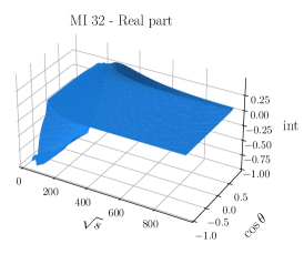
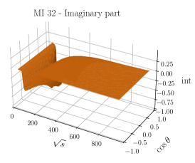
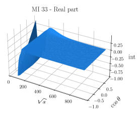
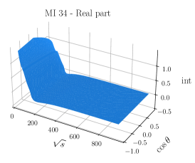
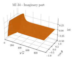
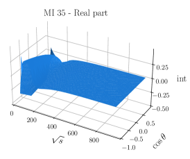
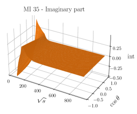
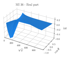
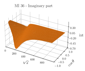
Figure 4: Real (left column) and imaginary (right column) parts of the $\epsilon^{0}$ coefficient of the two-mass MIs labeled 32 to 36 in ref. Bonciani:2016ypc .

In ref. Bonciani:2016ypc , 5 MIs with two internal massive lines have been solved in terms of Chen iterated integrals, but their analytical continuation to the physical region is extremely difficult. We thus turn to a different approach and we obtain these MIs in semi-analytical form, by solving the relevant system of differential equations via series expansion as initially proposed in ref. Moriello:2019yhu . This approach is implemented in the Mathematica code DiffExp Hidding:2020ytt . However, since the public version of DiffExp does not support, for the time being, the possibility of complex masses in the internal lines of the loop integrals, we have written an independent implementation of this procedure, that consistently takes into account the presence of complex weights and the analytic continuation to the complex plane SeaFire .

By approaching the problem in such semi-analytical way, we have to consider the complete system ($36\times 36$) of differential equations Bonciani:2016ypc , which includes the 5 MIs of eq. (51). The other 31 integrals are already known in terms of GHPLs and we use their numerical evaluation obtained with GiNaC Vollinga:2004sn as a cross check of the correct behaviour of our code finding perfect agreement. The values for the 5 MIs in eq. (51) are instead new predictions. In the euclidean region, we have checked our results for these 5 MIs against the values computed with PySecDec Borowka:2017idc , with perfect agreement within the numerical precision of PySecDec. In the physical region such comparison can not be performed, because of convergence issues observed with PySecDec, and we have adopted a different strategy. We have solved the same system of differential equations with a real value for the gauge-boson masses, by using both DiffExp and our private implementation, finding perfect agreement, for different values of the centre-of-mass energy, below and above all the physical thresholds.

In Figure 4 we present the real and imaginary parts of the values of the $\epsilon^{0}$ coefficient of the MIs numbered from 32 to 36 in ref. Bonciani:2016ypc , in a phase-space region relevant for LHC phenomenology. As a technical benchmark we provide in eqs. (5.2) the values of these five integrals, at $\sqrt{s}=120$ GeV and $\cos\theta=0$, using the $Z$ boson complex mass with the values presented in the next section.

$$MI_{32} = (-0.1749432674210653458206641571672526693701$$

$$-0.08577133842383776228342363457748528348231\leavevmode\nobreak\ i)\frac{1}{\varepsilon}+$$

$$(-0.6880611799340122002547431584730743961212$$

$$-0.7172116087719097073815199889325839829478\leavevmode\nobreak\ i)$$

$$MI_{33} = (+0.04590321278523478276320861551168882058745$$

$$-0.001565827650440604122381753305492983831372\leavevmode\nobreak\ i)\frac{1}{\varepsilon^{2}}+$$

$$(-0.1020302461263331342976597396613145347408$$

$$+0.02750120560010053399615654731836551427554\leavevmode\nobreak\ i)\frac{1}{\varepsilon}+$$

$$(-0.9440798936974029538680877301057978456673$$

$$-0.7373834572088279116262037334972425113889\leavevmode\nobreak\ i)$$

$$MI_{34} = (-0.04296293184352405065819376225216006379338$$

$$+0.0009207027182454070378064541717970157008000\leavevmode\nobreak\ i)\frac{1}{\varepsilon^{2}}+$$

$$(+0.08602650524260701502345707352625809659972$$

$$-0.1041839205419216009927204337308113344692\leavevmode\nobreak\ i)\frac{1}{\varepsilon}+$$

$$(+0.6256624139686838528066374865168826034798$$

$$+0.2884434585316438395669902051016636313148\leavevmode\nobreak\ i)$$

$$MI_{35} = (-0.03978405113517657583808686702509598723620$$

$$+0.0002682033570842286848993717924773930706110\leavevmode\nobreak\ i)\frac{1}{\varepsilon^{2}}+$$

$$(-0.08594509272571227733490076066555616396611$$

$$-0.1071667563486545058940834480592238792738\leavevmode\nobreak\ i)\frac{1}{\varepsilon}+$$

$$(+0.1863097462278093777896412913148906045862$$

$$-0.1309746755875472477456608996344754633763\leavevmode\nobreak\ i)$$

$$MI_{36} = (+0.03722281743928349433413785307317038487389$$

$$+0.0002207346628993822499145750213845713169838\leavevmode\nobreak\ i)\frac{1}{\varepsilon^{2}}+$$

$$(+0.05861962174451141932860447142100263348096$$

$$+0.1128699536667789677655115587719042497769\leavevmode\nobreak\ i)\frac{1}{\varepsilon}+$$

$$(-0.2459055670537880464977311941324743072103$$

$$-0.004310307792522490155395154024385441988819\leavevmode\nobreak\ i)$$

This approach faces all the problems of the analytical continuation immediately from the analysis of the structure of the differential equations. If it is possible to expand the solution in a region around the boundary condition points, then the problem becomes of algebraic nature, i.e. we have to solve for all the coefficients of the various powers of the expansion variable. The system of differential equations of ref. Bonciani:2016ypc can be cast in dlog form and thus contains the complete information about the singularity structure of the problem, in particular the position of the branch points relevant in the discussion of the polylogarithmic functions present in the solution. This information can be exploited to control the analytic continuation when we extend the solution to an adjacent region, either non-physical or physical. We remark that complete control on the analytic continuation has been verified when letting vary one kinematical variable at the time, while the others are kept fixed.

5.3 Numerical results

In this Section, we present the numerical evaluation of our result, the finite IR-subtracted UV-renormalised hard function ${H}^{(1,1)}$. For every practical application, the evaluation in one phase-space point of the correction factor stemming from the two-loop ${\cal O}(\alpha\alpha_{s})\leavevmode\nobreak\$virtual corrections requires a cumbersome procedure. We consider it more convenient to prepare a numerical grid for ${H}^{(1,1)}$, covering all the phase-space values relevant for NC DY in a given fiducial volume and parameterised in terms of the partonic centre-of-mass energy $\sqrt{s}$ and scattering angle $\cos\theta$. We notice that the virtual correction, after the subtraction of all the IR enhanced factors, is a smooth, slowly varying function of $\sqrt{s}$ and $\cos\theta$. We have prepared a grid with a sampling based on the known behaviour of the NLO-EW distribution, with special care for the $Z$ resonance region, where a finer binning is necessary.

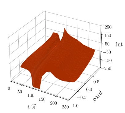
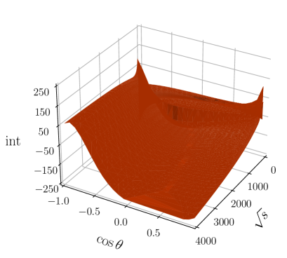
Figure 5: The contributions from all the vertex and box Feynman diagrams to the ${\cal O}(\alpha\alpha_{s})\leavevmode\nobreak\$correction to the finite hard function, in two different invariant mass ranges, as a function of $\sqrt{s}$ and $\cos\theta$.

For illustration purposes we consider here a grid with (130x25) points in $(\sqrt{s},\cos\theta)$, covering the intervals $s\in[40,13000]$ GeV and $\cos\theta\in[-1,1]$ and present the values in the ancillary file gridsth.m . The extraction of any intermediate value of ${H}^{(1,1)}$ can be obtained via interpolation of the grid points with excellent accuracy thanks to the smoothness of the function. With the sampling provided as ancillary file, we reproduce the exact correction with an accuracy at the $10^{-3}$ level, in the whole phase space. This accuracy is sufficient for phenomenological studies, but can be increased whenever needed.

The preparation, on a single core, of a grid of values for all the 36 two-masses MIs requires a fixed step, executed only once, to move from the boundary conditions fixed in the non-physical euclidean region to the physical region, which can take $\sim 20$ minutes. Moving in the physical region is faster, with an average time of $\sim 5$ minutes per point. Once this first grid is ready, the evaluation of the corresponding grid for the $H^{(1,1)}$ function requires $\sim 3$ minutes per point. Once the $H^{(1,1)}$ grid is ready, its interpolation in any simulation code requires a negligible time.

We use the following parameters:

$M_{Z}$	91.1535 GeV	$\Gamma_{Z}$	2.4943 GeV
$M_{W}$	80.358 GeV	$\Gamma_{W}$	2.084 GeV
$m_{H}$	125.09 GeV	$m_{t}$	173.07 GeV

The values of the gauge boson masses and decay widths are compatible with those reported in the PDG ParticleDataGroup:2020ssz , extracted in a running-width fitting scheme. The choice of the complex mass scheme to define the masses of the unstable $W$ and $Z$ bosons implies that all the functions which depend on these parameters become functions of complex variables. We have exploited the rescaling properties of the GHPLs to set their argument equal to one, adjusting all the other weights, which become in general complex. For the numerical evaluation of all the GHPLs appearing in the final expressions, we use GiNaC and handyG Naterop:2019xaf in two independent C++ and Mathematica codes to evaluate each phase-space point. We also use HarmonicSums Ablinger:2010kw ; Ablinger:2014rba , PolyLogTools Duhr:2019tlz and LoopTools Hahn:1998yk for several cross-checks of the one- and two-loop integrals available in closed analytic form, with real and complex masses. For the numerical evaluation of the 5 MIs of eq. (51), we use the semi-analytical approach described in Section 5.2.

We present in Figure 5 the numerical grid expressing the UV-renormalised IR-subtracted two-loop ${\cal O}(\alpha\alpha_{s})\leavevmode\nobreak\$virtual correction due to the two-loop vertex and box diagrams (Figure 1 a,b,f and Figure 2 a,b,f). The plots show the correction factor normalised to the Born cross section and expressed in units $\frac{\alpha}{\pi}\frac{\alpha_{s}}{\pi}$, as a function of $\sqrt{s}$ and $\cos\theta$. We consider the range $-1\leq\cos\theta\leq 1$ and, for the partonic center-of-mass energy, two different intervals, namely $50\leq\sqrt{s}\leq 250$ GeV and $50\leq\sqrt{s}\leq 5000$ GeV.

With the zoom in the $50\leq\sqrt{s}\leq 250$ GeV interval, we can appreciate the non-trivial structure of the corrections starting from the $Z$ resonance and up to 110 GeV. The description of the $WW$ and $ZZ$ thresholds is smooth, thanks to the implementation of the complex-mass scheme. Above 200 GeV the shape of the correction factor is negative, smooth, and slowly decreasing; we do not observe the appearance of additional structures. The non-trivial $\cos\theta$ dependence is due to parity violating effects, in largest size stemming from the interference between the two-loop $AA$ subset of diagrams and the tree-level amplitude with a $Z$-boson exchange.

6 Conclusions

In the NLO case, a complete automation of all the steps of the calculation is in a quite mature stage for both QCD and EW corrections. In the NNLO case instead, only parts of the procedure are automatic, because of various conceptual and computational problems. In this paper we have presented the details of the complete calculation of the exact ${\cal O}(\alpha\alpha_{s})\leavevmode\nobreak\$virtual corrections to the NC DY process, describing how we have overcome the problems appearing in the different stages of the procedure that brings us from the Feynman diagrams to the numerical evaluation of the squared matrix element.

All the algebraic manipulation processes face the difficulty of dealing with potentially very large expressions, so that a systematic simplification work, based on the search for recurring patterns, is crucial to keep the size of the formulae at a manageable level. While the reduction to MIs is completely standardised, the analytical subtraction of the IR divergences is not mature at the same level, and we have achieved this successful check only via a dedicated calculation. The presence of internal massive lines yields a rich analytical structure of the Feynman integrals; for the evaluation of the two-loop boxes with two massive lines we have adopted a semi-analytical approach, valid for arbitrary complex masses.

The final correction factor, defined in the $q_{T}$-subtraction scheme, has been cast in a relatively compact form, which we provide in the ancillary files. This finite virtual factor can be used in any simulation code, provided that the appropriate finite correction for the IR subtraction scheme is applied. For benchmarking we provide the grid with the numerical evaluation of the correction factor in the phase-space region relevant at the LHC.

The successful completion of all these steps can help to devise new strategies for the automation of the calculation of two-loop EW and mixed QCD-EW radiative corrections, relevant for processes at the LHC and future lepton colliders.

Appendix A Description of the ancillary files

In this subsection we present a description of the content of the ancillary files attached to the paper. A complete listing of all the symbols used in the analytical expressions and their correspondence with the physical quantities can be found in the README file.

In the ancillary Mathematica file NCDY_ME11.m, we present $\langle{\cal M}^{(0)}|{\cal M}^{(1,1),fin}\rangle$ i.e. the finite IR subtracted and UV renormalised matrix elements of all the vertex and box type Feynman diagrams. As discussed earlier, we present the result in the small lepton mass limit i.e. dropping all the terms which vanish as $m_{l}\rightarrow 0$. In the ancillary file uU_totaldelta_vertbox.dat, we provide the numerical evaluation, for up-type quark initiated channel, of the expressions contained in NCDY_ME11.m, divided by Born, multiplied by 2, divided by 16 and also subtracted of the logarithms of the lepton mass, using the numerical value of the input parameters as described in Section 5.3, for all the points of the grid specified in gridsth.m. We also provide the exact result including the full dependence of the lepton mass in ME11_partml_exact.m for the following subsets: all the vertex and box type contributions for the $\gamma\gamma$ subset and the contributions from the Feynman diagrams with NLO QED correction to the lepton vertex in the $\gamma Z$ subset. The explicit expressions of the two-loop self energy and one-loop self energy with NLO QCD contributions, are known in the literature (cfr. Refs. Dittmaier:2020vra and Refs. Denner:1991kt ). Hence, we refrain ourselves from providing these results.

The results are written as a combination of GHPLs and of the symbols associated to the MIs whose solution has been obtained via a semi-analytical method. Several variables have been introduced to define the weights and arguments of the GHPLs, which we report here for the sake of definiteness. Extending the notation of eq. (43), the Landau variables $x_{m}$ are defined with respect to the mass $m$ as follows,

$$\frac{(1-x_{m})^{2}}{x_{m}}=-\frac{s}{m^{2}}$$ (53)

where $m\in\{m_{l},\mu_{\scriptscriptstyle Z},\mu_{\scriptscriptstyle W}\}$. The kinematical ratios are defined as

$$\bar{x}_{m}=-\frac{s}{m^{2}}\,,\leavevmode\nobreak\ \leavevmode\nobreak\ y_{m}=-\frac{t}{m^{2}}\,,\leavevmode\nobreak\ \leavevmode\nobreak\ z_{m}=-\frac{u}{m^{2}}\,.$$ (54)

We define other variables $v_{m}$ and $v_{m}^{{}^{\prime}}$ as follows

$$-\frac{t}{m^{2}}=\frac{x_{m}}{v_{m}}\frac{(1+v_{m})^{2}}{(1+x_{m})^{2}}\,,\quad-\frac{u}{m^{2}}=\frac{x_{m}}{v_{m}^{{}^{\prime}}}\frac{(1+v_{m}^{{}^{\prime}})^{2}}{(1+x_{m})^{2}}\,.$$ (55)

The arguments of the GHPLs in the expressions have been reduced to 1 (denoted by ‘one’). The GHPLs are expressed as

$$G[a\_\_,1]\equiv L[\{a\},\mathsf{one}]\,.$$ (56)

The coefficients of $\epsilon^{n}$ of the series expansion in $\epsilon$ of the 5 MIs of eq. (51) for topology $B_{16}$ with $\mu_{V}=\mu_{\scriptscriptstyle Z}$ are denoted by

$$\mathsf{B16z[I32,n]},\mathsf{B16z[I33,n]},\mathsf{B16z[I34,n]},\mathsf{B16z[I35,n]},\mathsf{B16z[I36,n]}\,.$$ (57)

For topology $B_{16p}$ with $\mu_{V}=\mu_{\scriptscriptstyle Z}$, they are denoted by

$$\mathsf{B16zp[I32,n]},\mathsf{B16zp[I33,n]},\mathsf{B16zp[I34,n]},\mathsf{B16zp[I35,n]},\mathsf{B16zp[I36,n]}\,.$$ (58)

For topology $B_{16p}$ with $\mu_{V}=\mu_{\scriptscriptstyle W}$, they are denoted by

$$\mathsf{B16wp[I32,n]},\mathsf{B16wp[I33,n]},\mathsf{B16wp[I34,n]},\mathsf{B16wp[I35,n]},\mathsf{B16wp[I36,n]}\,.$$ (59)

The result also contains the one-loop box integral with two massive lines (Figure 5-${\cal T}_{6}$ of ref. Bonciani:2016ypc ) symbolically. We denote the $\epsilon^{n}$ coefficient of this one-loop box integral as

$$\mathsf{A16z[I6,n]},\mathsf{A16zp[I6,n]},\mathsf{A16wp[I6,n]}$$ (60)

where the one-loop topologies are defined by

$${\rm A}_{16} :\{{\cal D}_{1}-\mu_{V}^{2},{\cal D}_{1;1},{\cal D}_{1;12}-\mu_{V}^{2},{\cal D}_{1;3}\}$$

$${\rm A}_{16p} :\{{\cal D}_{1}-\mu_{V}^{2},{\cal D}_{1;2},{\cal D}_{1;12}-\mu_{V}^{2},{\cal D}_{1;3}\}\,.$$ (61)

The representation of the coupling constants and charges in the expressions is detailed below. $C_{v,f}$ and $C_{a,f}$ are the charges of the coupling of the Z boson to a fermion $f$. They are given by

$$C_{v,f}=\left(\frac{I_{W}^{(f)}}{2}-Q_{f}\,\sin\theta_{W}\right)\,,\leavevmode\nobreak\ \leavevmode\nobreak\ \leavevmode\nobreak\ C_{a,f}=\left(\frac{I_{W}^{(f)}}{2}\right)\,.$$ (62)

$I_{W}^{(f)}$ and $Q_{f}$ are the third component of the weak isospin and the electric charge in units of the positron charge, respectively. $\theta_{W}$ is the weak mixing angle. The following symbols and abbreviations are used throughout the files.

$$\mathsf{asr}=\frac{\alpha_{s}}{4\pi};\leavevmode\nobreak\ \leavevmode\nobreak\ \mathsf{aem}=\frac{\alpha}{4\pi};\leavevmode\nobreak\ \leavevmode\nobreak\ \mathsf{borncf}=N_{C};\leavevmode\nobreak\ \leavevmode\nobreak\ \mathsf{Cf}=C_{F};\leavevmode\nobreak\ \leavevmode\nobreak\ \mathsf{gA4}=e^{4};\leavevmode\nobreak\ \leavevmode\nobreak\$$

$$\mathsf{Qu}=Q_{u};\leavevmode\nobreak\ \leavevmode\nobreak\ \leavevmode\nobreak\ \mathsf{Qd}=Q_{d};\leavevmode\nobreak\ \leavevmode\nobreak\ \leavevmode\nobreak\ \mathsf{Ql}=Q_{l};\leavevmode\nobreak\ \leavevmode\nobreak\ \leavevmode\nobreak\$$

$$\mathsf{gVu}=C_{v,u};\leavevmode\nobreak\ \leavevmode\nobreak\ \mathsf{gAu}=C_{a,u};\leavevmode\nobreak\ \leavevmode\nobreak\ \mathsf{gVd}=C_{v,d};\leavevmode\nobreak\ \leavevmode\nobreak\ \mathsf{gAd}=C_{a,d};\leavevmode\nobreak\ \leavevmode\nobreak\$$

$$\mathsf{gVl}=C_{v,l};\leavevmode\nobreak\ \leavevmode\nobreak\ \mathsf{gAl}=C_{a,l};\leavevmode\nobreak\ \leavevmode\nobreak\ \mathsf{gVn}=C_{v,n};\leavevmode\nobreak\ \leavevmode\nobreak\ \mathsf{gAn}=C_{a,n};\leavevmode\nobreak\ \leavevmode\nobreak\$$ (63)

gVuC, gAuC, gVlC, gAlC are complex conjugate of gVu, gAu, gVl, gAl, respectively. The following constants appear in the expressions

$$\mathsf{pi}=\pi;\leavevmode\nobreak\ \leavevmode\nobreak\ \mathsf{IPi}=i\pi;\leavevmode\nobreak\ \leavevmode\nobreak\ \mathsf{z2}=\zeta_{2};\leavevmode\nobreak\ \leavevmode\nobreak\ \mathsf{z3}=\zeta_{3};\mathsf{c}=\frac{1}{2}+i\frac{\sqrt{3}}{2};\leavevmode\nobreak\ \mathsf{cb}=\frac{1}{2}-i\frac{\sqrt{3}}{2};$$ (64)

The presentation of the variables appearing in the expression is as follows:

$$\mathsf{xrl}=\bar{x}_{m_{l}};\leavevmode\nobreak\ \leavevmode\nobreak\ \leavevmode\nobreak\ \mathsf{xl}=x_{m_{l}};\leavevmode\nobreak\ \leavevmode\nobreak\ \leavevmode\nobreak\ \mathsf{yl}=y_{m_{l}};\leavevmode\nobreak\ \leavevmode\nobreak\ \leavevmode\nobreak\ \mathsf{zl}=z_{m_{l}};\leavevmode\nobreak\ \leavevmode\nobreak\ \leavevmode\nobreak\$$

$$\mathsf{xrZ}=\bar{x}_{\mu_{\scriptscriptstyle Z}};\leavevmode\nobreak\ \leavevmode\nobreak\ \leavevmode\nobreak\ \mathsf{xZ}=x_{\mu_{\scriptscriptstyle Z}};\leavevmode\nobreak\ \leavevmode\nobreak\ \leavevmode\nobreak\ \mathsf{yZ}=y_{\mu_{\scriptscriptstyle Z}};\leavevmode\nobreak\ \leavevmode\nobreak\ \leavevmode\nobreak\ \mathsf{zZ}=z_{\mu_{\scriptscriptstyle Z}};\leavevmode\nobreak\ \leavevmode\nobreak\ \leavevmode\nobreak\ \mathsf{vZ}=v_{\mu_{\scriptscriptstyle Z}};\leavevmode\nobreak\ \leavevmode\nobreak\ \leavevmode\nobreak\ \mathsf{vpZ}=v^{{}^{\prime}}_{\mu_{\scriptscriptstyle Z}};\leavevmode\nobreak\ \leavevmode\nobreak\ \leavevmode\nobreak\$$

$$\mathsf{xrW}=\bar{x}_{\mu_{\scriptscriptstyle W}};\leavevmode\nobreak\ \leavevmode\nobreak\ \mathsf{xW}=x_{\mu_{\scriptscriptstyle W}};\leavevmode\nobreak\ \leavevmode\nobreak\ \mathsf{yW}=y_{\mu_{\scriptscriptstyle W}};\leavevmode\nobreak\ \leavevmode\nobreak\ \mathsf{zW}=z_{\mu_{\scriptscriptstyle W}};\leavevmode\nobreak\ \leavevmode\nobreak\ \mathsf{vW}=v_{\mu_{\scriptscriptstyle W}};\leavevmode\nobreak\ \leavevmode\nobreak\ \mathsf{vpW}=v^{{}^{\prime}}_{\mu_{\scriptscriptstyle W}};$$

$$\mathsf{isqvZ}=i\sqrt{v_{\mu_{\scriptscriptstyle Z}}};\leavevmode\nobreak\ \leavevmode\nobreak\ \leavevmode\nobreak\ \mathsf{isqvpZ}=i\sqrt{v^{{}^{\prime}}_{\mu_{\scriptscriptstyle Z}}};\leavevmode\nobreak\ \leavevmode\nobreak\ \leavevmode\nobreak\ \mathsf{isqvW}=i\sqrt{v_{\mu_{\scriptscriptstyle W}}};\leavevmode\nobreak\ \leavevmode\nobreak\ \mathsf{isqvpW}=i\sqrt{v^{{}^{\prime}}_{\mu_{\scriptscriptstyle W}}};$$

$$\mathsf{cBpropml}=\frac{m_{l}^{2}}{s-\bar{\mu}_{{\scriptscriptstyle Z}}^{2}};\leavevmode\nobreak\ \mathsf{cBpropmZ}=\frac{\mu_{\scriptscriptstyle Z}^{2}}{s-\bar{\mu}_{{\scriptscriptstyle Z}}^{2}};\leavevmode\nobreak\ \mathsf{cBpropmW}=\frac{\mu_{\scriptscriptstyle W}^{2}}{s-\bar{\mu}_{{\scriptscriptstyle Z}}^{2}};$$ (65)

$\bar{\mu}_{{\scriptscriptstyle Z}}$ is the complex conjugate of $\mu_{\scriptscriptstyle Z}$.

References

- (1) S. Drell and T.-M. Yan, Massive Lepton Pair Production in Hadron-Hadron Collisions at High-Energies, Phys. Rev. Lett. 25 (1970) 316–320.
- (2) UA1 collaboration, G. Arnison et al., Experimental Observation of Isolated Large Transverse Energy Electrons with Associated Missing Energy at GeV, Phys. Lett. B 122 (1983) 103–116.
- (3) UA2 collaboration, M. Banner et al., Observation of Single Isolated Electrons of High Transverse Momentum in Events with Missing Transverse Energy at the CERN anti-p p Collider, Phys. Lett. B 122 (1983) 476–485.
- (4) UA1 collaboration, G. Arnison et al., Experimental Observation of Lepton Pairs of Invariant Mass Around 95-GeV/c**2 at the CERN SPS Collider, Phys. Lett. B 126 (1983) 398–410.
- (5) UA2 collaboration, P. Bagnaia et al., Evidence for at the CERN Collider, Phys. Lett. B 129 (1983) 130–140.
- (6) CDF, D0 collaboration, T. E. W. Group, 2012 Update of the Combination of CDF and D0 Results for the Mass of the W Boson, 1204.0042.
- (7) ATLAS collaboration, M. Aaboud et al., Measurement of the -boson mass in pp collisions at TeV with the ATLAS detector, Eur. Phys. J. C 78 (2018) 110, [1701.07240].
- (8) CDF, D0 collaboration, T. A. Aaltonen et al., Tevatron Run II combination of the effective leptonic electroweak mixing angle, Phys. Rev. D 97 (2018) 112007, [1801.06283].
- (9) ATLAS collaboration, Measurement of the effective leptonic weak mixing angle using electron and muon pairs from -boson decay in the ATLAS experiment at TeV, ATLAS-CONF-2018-037 (7, 2018) .
- (10) C. M. Carloni Calame, M. Chiesa, H. Martinez, G. Montagna, O. Nicrosini, F. Piccinini and A. Vicini, Precision Measurement of the W-Boson Mass: Theoretical Contributions and Uncertainties, Phys. Rev. D 96 (2017) 093005, [1612.02841].
- (11) E. Bagnaschi and A. Vicini, Parton Density Uncertainties and the Determination of Electroweak Parameters at Hadron Colliders, Phys. Rev. Lett. 126 (2021) 041801, [1910.04726].
- (12) A. Behring, F. Buccioni, F. Caola, M. Delto, M. Jaquier, K. Melnikov and R. Röntsch, Estimating the impact of mixed QCD-electroweak corrections on the -mass determination at the LHC, Phys. Rev. D 103 (2021) 113002, [2103.02671].
- (13) G. Altarelli, R. Ellis and G. Martinelli, Large Perturbative Corrections to the Drell-Yan Process in QCD, Nucl. Phys. B 157 (1979) 461–497.
- (14) R. Hamberg, W. van Neerven and T. Matsuura, A complete calculation of the order correction to the Drell-Yan factor, Nucl. Phys. B 359 (1991) 343–405.
- (15) R. V. Harlander and W. B. Kilgore, Next-to-next-to-leading order Higgs production at hadron colliders, Phys. Rev. Lett. 88 (2002) 201801, [hep-ph/0201206].
- (16) C. Duhr, F. Dulat and B. Mistlberger, Drell-Yan Cross Section to Third Order in the Strong Coupling Constant, Phys. Rev. Lett. 125 (2020) 172001, [2001.07717].
- (17) C. Duhr, F. Dulat and B. Mistlberger, Charged current Drell-Yan production at N3LO, JHEP 11 (2020) 143, [2007.13313].
- (18) C. Duhr and B. Mistlberger, Lepton-pair production at hadron colliders at N3LO in QCD, JHEP 03 (2022) 116, [2111.10379].
- (19) C. Anastasiou, L. J. Dixon, K. Melnikov and F. Petriello, Dilepton rapidity distribution in the Drell-Yan process at NNLO in QCD, Phys. Rev. Lett. 91 (2003) 182002, [hep-ph/0306192].
- (20) C. Anastasiou, L. J. Dixon, K. Melnikov and F. Petriello, High precision QCD at hadron colliders: Electroweak gauge boson rapidity distributions at NNLO, Phys. Rev. D 69 (2004) 094008, [hep-ph/0312266].
- (21) K. Melnikov and F. Petriello, Electroweak gauge boson production at hadron colliders through , Phys. Rev. D 74 (2006) 114017, [hep-ph/0609070].
- (22) S. Catani, L. Cieri, G. Ferrera, D. de Florian and M. Grazzini, Vector boson production at hadron colliders: a fully exclusive QCD calculation at NNLO, Phys. Rev. Lett. 103 (2009) 082001, [0903.2120].
- (23) S. Catani, G. Ferrera and M. Grazzini, W Boson Production at Hadron Colliders: The Lepton Charge Asymmetry in NNLO QCD, JHEP 05 (2010) 006, [1002.3115].
- (24) S. Camarda, L. Cieri and G. Ferrera, Drell–Yan lepton-pair production: qT resummation at N3LL accuracy and fiducial cross sections at N3LO, Phys. Rev. D 104 (2021) L111503, [2103.04974].
- (25) S. Moch and A. Vogt, Higher-order soft corrections to lepton pair and Higgs boson production, Phys. Lett. B 631 (2005) 48–57, [hep-ph/0508265].
- (26) E. Laenen and L. Magnea, Threshold resummation for electroweak annihilation from DIS data, Phys. Lett. B 632 (2006) 270–276, [hep-ph/0508284].
- (27) V. Ravindran, On Sudakov and soft resummations in QCD, Nucl. Phys. B 746 (2006) 58–76, [hep-ph/0512249].
- (28) V. Ravindran, Higher-order threshold effects to inclusive processes in QCD, Nucl. Phys. B 752 (2006) 173–196, [hep-ph/0603041].
- (29) D. de Florian and J. Mazzitelli, A next-to-next-to-leading order calculation of soft-virtual cross sections, JHEP 12 (2012) 088, [1209.0673].
- (30) T. Ahmed, M. Mahakhud, N. Rana and V. Ravindran, Drell-Yan Production at Threshold to Third Order in QCD, Phys. Rev. Lett. 113 (2014) 112002, [1404.0366].
- (31) S. Catani, L. Cieri, D. de Florian, G. Ferrera and M. Grazzini, Threshold resummation at N3LL accuracy and soft-virtual cross sections at N3LO, Nucl. Phys. B 888 (2014) 75–91, [1405.4827].
- (32) Y. Li, A. von Manteuffel, R. M. Schabinger and H. X. Zhu, Soft-virtual corrections to Higgs production at N3LO, Phys. Rev. D 91 (2015) 036008, [1412.2771].
- (33) A. H. Ajjath, P. Mukherjee and V. Ravindran, On next to soft corrections to Drell-Yan and Higgs Boson productions, 2006.06726.
- (34) S. Dittmaier and M. Krämer, Electroweak radiative corrections to W boson production at hadron colliders, Phys. Rev. D 65 (2002) 073007, [hep-ph/0109062].
- (35) U. Baur and D. Wackeroth, Electroweak radiative corrections to beyond the pole approximation, Phys. Rev. D 70 (2004) 073015, [hep-ph/0405191].
- (36) V. Zykunov, Radiative corrections to the Drell-Yan process at large dilepton invariant masses, Phys. Atom. Nucl. 69 (2006) 1522.
- (37) A. Arbuzov, D. Bardin, S. Bondarenko, P. Christova, L. Kalinovskaya, G. Nanava and R. Sadykov, One-loop corrections to the Drell-Yan process in SANC. I. The Charged current case, Eur. Phys. J. C 46 (2006) 407–412, [hep-ph/0506110].
- (38) C. Carloni Calame, G. Montagna, O. Nicrosini and A. Vicini, Precision electroweak calculation of the charged current Drell-Yan process, JHEP 12 (2006) 016, [hep-ph/0609170].
- (39) U. Baur, O. Brein, W. Hollik, C. Schappacher and D. Wackeroth, Electroweak radiative corrections to neutral current Drell-Yan processes at hadron colliders, Phys. Rev. D 65 (2002) 033007, [hep-ph/0108274].
- (40) V. Zykunov, Weak radiative corrections to Drell-Yan process for large invariant mass of di-lepton pair, Phys. Rev. D 75 (2007) 073019, [hep-ph/0509315].
- (41) C. Carloni Calame, G. Montagna, O. Nicrosini and A. Vicini, Precision electroweak calculation of the production of a high transverse-momentum lepton pair at hadron colliders, JHEP 10 (2007) 109, [0710.1722].
- (42) A. Arbuzov, D. Bardin, S. Bondarenko, P. Christova, L. Kalinovskaya, G. Nanava and R. Sadykov, One-loop corrections to the Drell–Yan process in SANC. (II). The Neutral current case, Eur. Phys. J. C 54 (2008) 451–460, [0711.0625].
- (43) S. Dittmaier and M. Huber, Radiative corrections to the neutral-current Drell-Yan process in the Standard Model and its minimal supersymmetric extension, JHEP 01 (2010) 060, [0911.2329].
- (44) G. Balossini, G. Montagna, C. M. Carloni Calame, M. Moretti, O. Nicrosini, F. Piccinini, M. Treccani and A. Vicini, Combination of electroweak and QCD corrections to single W production at the Fermilab Tevatron and the CERN LHC, JHEP 01 (2010) 013, [0907.0276].
- (45) C. Bernaciak and D. Wackeroth, Combining NLO QCD and Electroweak Radiative Corrections to W boson Production at Hadron Colliders in the POWHEG Framework, Phys. Rev. D 85 (2012) 093003, [1201.4804].
- (46) L. Barze, G. Montagna, P. Nason, O. Nicrosini and F. Piccinini, Implementation of electroweak corrections in the POWHEG BOX: single W production, JHEP 04 (2012) 037, [1202.0465].
- (47) L. Barze, G. Montagna, P. Nason, O. Nicrosini, F. Piccinini and A. Vicini, Neutral current Drell-Yan with combined QCD and electroweak corrections in the POWHEG BOX, Eur. Phys. J. C 73 (2013) 2474, [1302.4606].
- (48) R. Frederix, S. Frixione, V. Hirschi, D. Pagani, H. S. Shao and M. Zaro, The automation of next-to-leading order electroweak calculations, JHEP 07 (2018) 185, [1804.10017].
- (49) D. de Florian, M. Der and I. Fabre, QCDQED NNLO corrections to Drell Yan production, Phys. Rev. D 98 (2018) 094008, [1805.12214].
- (50) L. Cieri, D. de Florian, M. Der and J. Mazzitelli, Mixed QCDQED corrections to exclusive Drell Yan production using the qT -subtraction method, JHEP 09 (2020) 155, [2005.01315].
- (51) M. Delto, M. Jaquier, K. Melnikov and R. Röntsch, Mixed QCDQED corrections to on-shell boson production at the LHC, JHEP 01 (2020) 043, [1909.08428].
- (52) R. Bonciani, F. Buccioni, R. Mondini and A. Vicini, Double-real corrections at to single gauge boson production, Eur. Phys. J. C 77 (2017) 187, [1611.00645].
- (53) R. Bonciani, F. Buccioni, N. Rana, I. Triscari and A. Vicini, NNLO QCDEW corrections to Z production in the channel, Phys. Rev. D 101 (2020) 031301, [1911.06200].
- (54) R. Bonciani, F. Buccioni, N. Rana and A. Vicini, NNLO QCDEW corrections to on-shell production, Phys. Rev. Lett. 125 (2020) 232004, [2007.06518].
- (55) R. Bonciani, F. Buccioni, N. Rana and A. Vicini, On-shell Z boson production at hadron colliders through (s), JHEP 02 (2022) 095, [2111.12694].
- (56) F. Buccioni, F. Caola, M. Delto, M. Jaquier, K. Melnikov and R. Röntsch, Mixed QCD-electroweak corrections to on-shell Z production at the LHC, Phys. Lett. B 811 (2020) 135969, [2005.10221].
- (57) A. Behring, F. Buccioni, F. Caola, M. Delto, M. Jaquier, K. Melnikov and R. Röntsch, Mixed QCD-electroweak corrections to -boson production in hadron collisions, Phys. Rev. D 103 (2021) 013008, [2009.10386].
- (58) A. Denner and S. Dittmaier, Electroweak Radiative Corrections for Collider Physics, Phys. Rept. 864 (2020) 1–163, [1912.06823].
- (59) S. Dittmaier, A. Huss and C. Schwinn, Mixed QCD-electroweak corrections to Drell-Yan processes in the resonance region: pole approximation and non-factorizable corrections, Nucl. Phys. B 885 (2014) 318–372, [1403.3216].
- (60) S. Dittmaier, A. Huss and C. Schwinn, Dominant mixed QCD-electroweak O(s) corrections to Drell–Yan processes in the resonance region, Nucl. Phys. B 904 (2016) 216–252, [1511.08016].
- (61) S. Dittmaier, T. Schmidt and J. Schwarz, Mixed NNLO QCDelectroweak corrections of to single-W/Z production at the LHC, JHEP 12 (2020) 201, [2009.02229].
- (62) L. Buonocore, M. Grazzini, S. Kallweit, C. Savoini and F. Tramontano, Mixed QCD-EW corrections to at the LHC, Phys. Rev. D 103 (2021) 114012, [2102.12539].
- (63) R. Bonciani, L. Buonocore, M. Grazzini, S. Kallweit, N. Rana, F. Tramontano and A. Vicini, Mixed Strong-Electroweak Corrections to the Drell-Yan Process, Phys. Rev. Lett. 128 (2022) 012002, [2106.11953].
- (64) L. Buonocore, S. Kallweit, L. Rottoli and M. Wiesemann, Linear power corrections for two-body kinematics in the subtraction formalism, 2111.13661.
- (65) S. Camarda, L. Cieri and G. Ferrera, Fiducial perturbative power corrections within the qT subtraction formalism, 2111.14509.
- (66) R. Bonciani, S. Di Vita, P. Mastrolia and U. Schubert, Two-Loop Master Integrals for the mixed EW-QCD virtual corrections to Drell-Yan scattering, JHEP 09 (2016) 091, [1604.08581].
- (67) M. Heller, A. von Manteuffel and R. M. Schabinger, Multiple polylogarithms with algebraic arguments and the two-loop EW-QCD Drell-Yan master integrals, Phys. Rev. D 102 (2020) 016025, [1907.00491].
- (68) S. M. Hasan and U. Schubert, Master Integrals for the mixed QCD-QED corrections to the Drell-Yan production of a massive lepton pair, JHEP 11 (2020) 107, [2004.14908].
- (69) M.-M. Long, R.-Y. Zhang, W.-G. Ma, Y. Jiang, L. Han, Z. Li and S.-S. Wang, Master integrals for mixed QCD-QED corrections to charged-current Drell-Yan production of a massive charged lepton, 2111.14130.
- (70) M. Heller, A. von Manteuffel, R. M. Schabinger and H. Spiesberger, Mixed EW-QCD two-loop amplitudes for and scheme independence of multi-loop corrections, JHEP 05 (2021) 213, [2012.05918].
- (71) F. V. Tkachov, A Theorem on Analytical Calculability of Four Loop Renormalization Group Functions, Phys. Lett. B 100 (1981) 65–68.
- (72) K. G. Chetyrkin and F. V. Tkachov, Integration by Parts: The Algorithm to Calculate beta Functions in 4 Loops, Nucl. Phys. B 192 (1981) 159–204.
- (73) T. Gehrmann and E. Remiddi, Differential equations for two loop four point functions, Nucl. Phys. B580 (2000) 485–518, [hep-ph/9912329].
- (74) G. ’t Hooft and M. J. G. Veltman, Regularization and Renormalization of Gauge Fields, Nucl. Phys. B 44 (1972) 189–213.
- (75) D. Kreimer, The (5) Problem and Anomalies: A Clifford Algebra Approach, Phys. Lett. B 237 (1990) 59–62.
- (76) J. G. Korner, D. Kreimer and K. Schilcher, A Practicable gamma(5) scheme in dimensional regularization, Z. Phys. C 54 (1992) 503–512.
- (77) M. Chiesa, F. Piccinini and A. Vicini, Direct determination of at hadron colliders, Phys. Rev. D 100 (2019) 071302, [1906.11569].
- (78) G. Degrassi and A. Vicini, Two loop renormalization of the electric charge in the standard model, Phys. Rev. D69 (2004) 073007, [hep-ph/0307122].
- (79) A. Denner, S. Dittmaier, M. Roth and L. H. Wieders, Electroweak corrections to charged-current e+ e- — 4 fermion processes: Technical details and further results, Nucl. Phys. B 724 (2005) 247–294, [hep-ph/0505042].
- (80) A. Sirlin, Radiative Corrections in the SU(2)-L x U(1) Theory: A Simple Renormalization Framework, Phys. Rev. D22 (1980) 971–981.
- (81) B. A. Kniehl, Two Loop Corrections to the Vacuum Polarizations in Perturbative QCD, Nucl. Phys. B 347 (1990) 86–104.
- (82) A. Djouadi and P. Gambino, Electroweak gauge bosons selfenergies: Complete QCD corrections, Phys. Rev. D 49 (1994) 3499–3511, [hep-ph/9309298].
- (83) A. Denner, G. Weiglein and S. Dittmaier, Application of the background field method to the electroweak standard model, Nucl. Phys. B 440 (1995) 95–128, [hep-ph/9410338].
- (84) S. Catani, The Singular behavior of QCD amplitudes at two loop order, Phys. Lett. B 427 (1998) 161–171, [hep-ph/9802439].
- (85) P. Nogueira, Automatic Feynman graph generation, J. Comput. Phys. 105 (1993) 279–289.
- (86) T. Hahn, Generating Feynman diagrams and amplitudes with FeynArts 3, Comput. Phys. Commun. 140 (2001) 418–431, [hep-ph/0012260].
- (87) J. A. M. Vermaseren, New features of FORM, math-ph/0010025.
- (88) W. R. Inc., “Mathematica, Version 12.3.1.”
- (89) P. Maierhöfer, J. Usovitsch and P. Uwer, Kira—A Feynman integral reduction program, Comput. Phys. Commun. 230 (2018) 99–112, [1705.05610].
- (90) R. N. Lee, LiteRed 1.4: a powerful tool for reduction of multiloop integrals, J. Phys. Conf. Ser. 523 (2014) 012059, [1310.1145].
- (91) R. N. Lee, Presenting LiteRed: a tool for the Loop InTEgrals REDuction, 1212.2685.
- (92) A. von Manteuffel and C. Studerus, Reduze 2 - Distributed Feynman Integral Reduction, 1201.4330.
- (93) C. Studerus, Reduze-Feynman Integral Reduction in C++, Comput. Phys. Commun. 181 (2010) 1293–1300, [0912.2546].
- (94) J. Frenkel and J. C. Taylor, Exponentiation of Leading Infrared Divergences in Massless Yang-Mills Theories, Nucl. Phys. B 116 (1976) 185–194.
- (95) T. Gehrmann, T. Huber and D. Maitre, Two-loop quark and gluon form-factors in dimensional regularisation, Phys. Lett. B 622 (2005) 295–302, [hep-ph/0507061].
- (96) R. Bonciani, A. Ferroglia, T. Gehrmann, D. Maitre and C. Studerus, Two-Loop Fermionic Corrections to Heavy-Quark Pair Production: The Quark-Antiquark Channel, JHEP 07 (2008) 129, [0806.2301].
- (97) R. Bonciani, A. Ferroglia, T. Gehrmann and C. Studerus, Two-Loop Planar Corrections to Heavy-Quark Pair Production in the Quark-Antiquark Channel, JHEP 08 (2009) 067, [0906.3671].
- (98) U. Aglietti and R. Bonciani, Master integrals with one massive propagator for the two loop electroweak form-factor, Nucl. Phys. B 668 (2003) 3–76, [hep-ph/0304028].
- (99) U. Aglietti and R. Bonciani, Master integrals with 2 and 3 massive propagators for the 2 loop electroweak form-factor - planar case, Nucl. Phys. B 698 (2004) 277–318, [hep-ph/0401193].
- (100) S. Catani and M. H. Seymour, The Dipole formalism for the calculation of QCD jet cross-sections at next-to-leading order, Phys. Lett. B 378 (1996) 287–301, [hep-ph/9602277].
- (101) S. Catani and M. H. Seymour, A General algorithm for calculating jet cross-sections in NLO QCD, Nucl. Phys. B 485 (1997) 291–419, [hep-ph/9605323].
- (102) S. Catani, S. Dittmaier, M. H. Seymour and Z. Trocsanyi, The Dipole formalism for next-to-leading order QCD calculations with massive partons, Nucl. Phys. B 627 (2002) 189–265, [hep-ph/0201036].
- (103) S. Frixione, Z. Kunszt and A. Signer, Three jet cross-sections to next-to-leading order, Nucl. Phys. B 467 (1996) 399–442, [hep-ph/9512328].
- (104) Les Houches 2017: Physics at TeV Colliders Standard Model Working Group Report, 3, 2018.
- (105) G. F. Sterman and M. E. Tejeda-Yeomans, Multiloop amplitudes and resummation, Phys. Lett. B 552 (2003) 48–56, [hep-ph/0210130].
- (106) T. Becher and M. Neubert, Infrared singularities of scattering amplitudes in perturbative QCD, Phys. Rev. Lett. 102 (2009) 162001, [0901.0722].
- (107) E. Gardi and L. Magnea, Factorization constraints for soft anomalous dimensions in QCD scattering amplitudes, JHEP 03 (2009) 079, [0901.1091].
- (108) W. B. Kilgore and C. Sturm, Two-Loop Virtual Corrections to Drell-Yan Production at order , Phys. Rev. D 85 (2012) 033005, [1107.4798].
- (109) W. B. Kilgore, The Two-Loop Infrared Structure of Amplitudes with Mixed Gauge Groups, Eur. Phys. J. C 73 (2013) 2603, [1308.1055].
- (110) A. Mitov and S. Moch, The Singular behavior of massive QCD amplitudes, JHEP 05 (2007) 001, [hep-ph/0612149].
- (111) T. Becher and K. Melnikov, Two-loop QED corrections to Bhabha scattering, JHEP 06 (2007) 084, [0704.3582].
- (112) T. Becher and M. Neubert, Infrared singularities of QCD amplitudes with massive partons, Phys. Rev. D 79 (2009) 125004, [0904.1021].
- (113) T. Ahmed, J. M. Henn and M. Steinhauser, High energy behaviour of form factors, JHEP 06 (2017) 125, [1704.07846].
- (114) J. Blümlein, P. Marquard and N. Rana, Asymptotic behavior of the heavy quark form factors at higher order, Phys. Rev. D 99 (2019) 016013, [1810.08943].
- (115) S. Catani, M. Grazzini and A. Torre, Transverse-momentum resummation for heavy-quark hadroproduction, Nucl. Phys. B 890 (2014) 518–538, [1408.4564].
- (116) S. Catani, S. Devoto, M. Grazzini, S. Kallweit, J. Mazzitelli and H. Sargsyan, Top-quark pair hadroproduction at next-to-next-to-leading order in QCD, Phys. Rev. D 99 (2019) 051501, [1901.04005].
- (117) S. Catani, S. Devoto, M. Grazzini, S. Kallweit and J. Mazzitelli, Top-quark pair production at the LHC: Fully differential QCD predictions at NNLO, JHEP 07 (2019) 100, [1906.06535].
- (118) S. Catani, S. Devoto, M. Grazzini, S. Kallweit and J. Mazzitelli, Bottom-quark production at hadron colliders: fully differential predictions in NNLO QCD, JHEP 03 (2021) 029, [2010.11906].
- (119) L. Buonocore, M. Grazzini and F. Tramontano, The subtraction method: electroweak corrections and power suppressed contributions, Eur. Phys. J. C 80 (2020) 254, [1911.10166].
- (120) S. Catani and M. Grazzini, An NNLO subtraction formalism in hadron collisions and its application to Higgs boson production at the LHC, Phys. Rev. Lett. 98 (2007) 222002, [hep-ph/0703012].
- (121) A. V. Kotikov, Differential equations method: New technique for massive Feynman diagrams calculation, Phys. Lett. B 254 (1991) 158–164.
- (122) E. Remiddi, Differential equations for Feynman graph amplitudes, Nuovo Cim. A 110 (1997) 1435–1452, [hep-th/9711188].
- (123) M. Argeri and P. Mastrolia, Feynman Diagrams and Differential Equations, Int. J. Mod. Phys. A 22 (2007) 4375–4436, [0707.4037].
- (124) J. M. Henn, Lectures on differential equations for Feynman integrals, J. Phys. A 48 (2015) 153001, [1412.2296].
- (125) J. Ablinger, A. Behring, J. Blümlein, A. De Freitas, A. von Manteuffel and C. Schneider, Calculating Three Loop Ladder and V-Topologies for Massive Operator Matrix Elements by Computer Algebra, Comput. Phys. Commun. 202 (2016) 33–112, [1509.08324].
- (126) J. Ablinger, J. Blümlein, P. Marquard, N. Rana and C. Schneider, Automated Solution of First Order Factorizable Systems of Differential Equations in One Variable, Nucl. Phys. B 939 (2019) 253–291, [1810.12261].
- (127) A. Goncharov, Polylogarithms in arithmetic and geometry, Proceedings of the International Congress of Mathematicians 1,2 (1995) 374–387.
- (128) A. B. Goncharov, Multiple polylogarithms and mixed Tate motives, math/0103059.
- (129) E. Remiddi and J. Vermaseren, Harmonic polylogarithms, Int.J.Mod.Phys. A15 (2000) 725–754, [hep-ph/9905237].
- (130) K.-T. Chen, Iterated path integrals, Bull. Am. Math. Soc. 83 (1977) 831–879.
- (131) F. Moriello, Generalised power series expansions for the elliptic planar families of Higgs + jet production at two loops, JHEP 01 (2020) 150, [1907.13234].
- (132) M. Hidding, DiffExp, a Mathematica package for computing Feynman integrals in terms of one-dimensional series expansions, Comput. Phys. Commun. 269 (2021) 108125, [2006.05510].
- (133) T. Armadillo, R. Bonciani, S. Devoto, N. Rana and A. Vicini, in preparation.
- (134) J. Vollinga and S. Weinzierl, Numerical evaluation of multiple polylogarithms, Comput. Phys. Commun. 167 (2005) 177, [hep-ph/0410259].
- (135) S. Borowka, G. Heinrich, S. Jahn, S. P. Jones, M. Kerner, J. Schlenk and T. Zirke, pySecDec: a toolbox for the numerical evaluation of multi-scale integrals, Comput. Phys. Commun. 222 (2018) 313–326, [1703.09692].
- (136) Particle Data Group collaboration, P. A. Zyla et al., Review of Particle Physics, PTEP 2020 (2020) 083C01.
- (137) R. Bonciani, G. Degrassi and A. Vicini, On the Generalized Harmonic Polylogarithms of One Complex Variable, Comput. Phys. Commun. 182 (2011) 1253–1264, [1007.1891].
- (138) L. Naterop, A. Signer and Y. Ulrich, handyG —Rapid numerical evaluation of generalised polylogarithms in Fortran, Comput. Phys. Commun. 253 (2020) 107165, [1909.01656].
- (139) J. Ablinger, A Computer Algebra Toolbox for Harmonic Sums Related to Particle Physics, Master’s thesis, Linz U. (2009) , [1011.1176].
- (140) J. Ablinger, The package HarmonicSums: Computer Algebra and Analytic aspects of Nested Sums, PoS LL2014 (2014) 019, [1407.6180].
- (141) C. Duhr and F. Dulat, PolyLogTools — polylogs for the masses, JHEP 08 (2019) 135, [1904.07279].
- (142) T. Hahn and M. Perez-Victoria, Automatized one loop calculations in four-dimensions and D-dimensions, Comput. Phys. Commun. 118 (1999) 153–165, [hep-ph/9807565].
- (143) A. Denner, Techniques for calculation of electroweak radiative corrections at the one loop level and results for W physics at LEP-200, Fortsch. Phys. 41 (1993) 307–420, [0709.1075].