Unconditional Effects of General Policy Interventions

Abstract

This paper studies the unconditional effects of a general policy intervention, which includes location-scale shifts and simultaneous shifts as special cases. The location-scale shift is intended to study a counterfactual policy aimed at changing not only the mean or location of a covariate but also its dispersion or scale. The simultaneous shift refers to the situation where shifts in two or more covariates take place simultaneously. For example, a shift in one covariate is compensated at a certain rate by a shift in another covariate. Not accounting for these possible scale or simultaneous shifts will result in an incorrect assessment of the potential policy effects on an outcome variable of interest. The unconditional policy parameters are estimated with simple semiparametric estimators, for which asymptotic properties are studied. Monte Carlo simulations are implemented to study their finite sample performances. The proposed approach is applied to a Mincer equation to study the effects of changing years of education on wages and to study the effect of smoking during pregnancy on birth weight.

Keywords: Location-scale shift, quantile regression, simultaneous shift, unconditional policy effect, unconditional regression.

JEL: J01, J31.

1 Introduction

In many research areas, it is important to assess the distributional effects of covariates on an outcome variable. Several methods have been implemented in the literature to study this. A prolific line of research is a combination of conditional mean and quantile regression models together with micro simulation exercises, as in Autor, Katz, and Kearney (2005), Machado and Mata (1995), and Melly (2005) (see Fortin, Lemieux, and Firpo (2011) for a review). A more recent and popular method is the recentered influence function (RIF) regression of Firpo, Fortin, and Lemieux (2009), which directly estimates the effect of a change in the covariate distribution on a functional of the unconditional distribution of the outcome variable. The functional of interest can be the mean, quantile, or any other aspect of the unconditional distribution.

Consider, as an example, the unconditional quantile of the outcome variable $Y$. Let $F_{Y}$ be the unconditional distribution function of $Y,$ then the $\tau$-quantile of $F_{Y}$ is defined by

$$Q_{\tau}[Y]:=\arg\min\{q:\tau\leq F_{Y}(q)\}\ \ \mbox{for}\ \ \tau\in(0,1).$$

In this paper, we seek to study how $Q_{\tau}[Y]$ changes when we induce an infinitesimal change in a covariate $X\in\mathbb{R}$,  allowing the presence of other observable covariates $W$ and unobservable covariates collected in $U.$ These covariates and the outcome variable are related via a structural or causal function $h$ so that $Y=h(X,W,U)$. We consider a sequence of policy experiments that change $X$ into $X_{\delta}=\mathcal{G}(X;\delta)$ for a smooth function $\mathcal{G}(\cdot;\cdot)$. The policy experiments are indexed by $\delta$ satisfying $\mathcal{G}(X;0)=X.$ That is, $\delta=0$ corresponds to the status quo policy. With this induced change in $X$, the outcome variable becomes $Y_{\delta}=h(X_{\delta},W,U)=h(\mathcal{G}(X;\delta),W,U)$ where the distribution of $\left(X,W,U\right)$ is held constant. Our policy experiment has a ceteris paribus interpretation at the population level: we change $X$ into $X_{\delta}$ while holding the stochastic dependence among $X,W,$ and $U$ constant. Such a policy experiment is implementable if the covariate $X$ is not a causal factor for either $W$ or $U.$ In this case, when we intervene $X$ and change it into $X_{\delta}$, $W$ and $U$ will not change. This does not rule out the stochastic dependence among $X,$ $W,$ and $U.$ In the meanwhile, the structural function $h(\cdot,\cdot,\cdot)$ is also held constant. The main parameter of interest is the marginal effect of the change on the unconditional quantile of the outcome variable:

$$\Pi_{\tau}:=\lim_{\delta\rightarrow 0}\frac{Q_{\tau}[Y_{\delta}]-Q_{\tau}[Y]}{\delta}.$$

Firpo, Fortin, and Lemieux (2009) develop methods to study what corresponds to a location shift $X_{\delta}=X+\delta$. This shift affects the entire unconditional distribution of $Y=h(X,W,U)$, moving it towards a counterfactual distribution of $Y_{\delta}=h(X+\delta,W,U)$. One of the main results in Firpo, Fortin, and Lemieux (2009, p.958, eq. (6)) is that $\Pi_{\tau}$ can be represented as an average derivative:

$$\Pi_{\tau}=E\left[\dot{\psi}_{x}\left(X,W\right)\right],$$

where

$$\dot{\psi}_{x}\left(x,w\right)=\frac{\partial E\left[\psi\left(Y,\tau,F_{Y}\right)|X=x,W=w\right]}{\partial x},$$

$\psi\left(y,\tau,F_{Y}\right)=\left[\tau-1\left\{y\leq Q_{\tau}[Y]\right\}\right]/f_{Y}(Q_{\tau}[Y])$ is the influence function of the quantile functional, and $f_{Y}(Q_{\tau}[Y])$ is the unconditional density of $Y$ evaluated at the $\tau$-quantile $Q_{\tau}[Y].$ The unconditional quantile effect $\Pi_{\tau}$ can then be estimated by first running an unconditional quantile regression (henceforth, UQR), which involves regressing the influence function $\psi\left(Y_{i},\tau,F_{Y}\right)$ on the covariates $(X_{i},W_{i})$ and then taking an average of the partial derivatives of the regression function with respect to $X.$

The same method is applicable to other functionals of interest — we only need to replace $\psi\left(y,\tau,F_{Y}\right)$ by the influence function underlying the functional we care about. This leads to the general RIF regression of Firpo, Fortin, and Lemieux (2009). The potential simplicity and flexibility that the methodology offers motivates subsequent research to expand the use of RIF regressions. On the empirical side, after its introduction, RIF regressions became a popular method for analyzing and identifying the distributional effects on outcomes in terms of changes in observed characteristics in areas such as labor economics, income and inequality, health economics, and public policy. On the theoretical side, Rothe (2012) provides a generalization of Firpo, Fortin, and Lemieux (2009) for the case of location shifts, and, more recently, Sasaki, Ura, and Zhang (2020) study the high-dimensional setting while Inoue, Li, and Xu (2021) focus on the two-sample problem. An alternative estimation procedure is proposed in Alejo, Galvao, Martinez-Iriarte, and Montes-Rojas (2023).

This paper extends the UQR and RIF regression in several ways. First, we study general counterfactual policy changes, of which the location shift is a special case. Our framework allows for any smooth and invertible intervention of the target covariates. As a complement to the existing literature that focuses on changing the marginal distribution of the target covariates, we consider changing the values of the target covariates directly. An advantage of our approach is that the changes under consideration are directly implementable. We note that it may not be easy to induce a desired shift in the marginal distribution, and when possible, such a shift is often achieved via transforming the target covariates, which is what we consider here.

Second, we provide extensive discussions of a counterfactual policy that, in addition to the location shift, affects the scale of a covariate. For example, we may consider $X_{\delta}=X/(1+\delta)+\delta.$ We find that in this case, the marginal effect can be decomposed as the sum of two effects: one related to the location shift and the other related to the scale shift. In order to interpret the scale effect, we introduce the quantile-standard deviation elasticity: the percentage change in the unconditional quantiles of the outcome variable induced by a 1% change in the standard deviation of the target covariate.

Third, we allow the target covariates to be endogenous, and we characterize the asymptotic bias of the unconditional effect estimator when the endogeneity is not appropriately accounted for. We eliminate the endogeneity bias using a control variable/function approach. Such an approach is analogous to the method of causal inference under the unconfoundedness assumption.

Fourth, by letting the policy function depend on covariates so that $X_{\delta}=\mathcal{G}(X,W;\delta)$, we allow the interventions to vary across covariate-specific strata. In the Supplemental Appendix, we also consider the case of simultaneous shifts in different covariates. We focus on the case of simultaneous location shifts in two covariates. This happens when a location shift in one covariate induces a location shift in another covariate at the same time. For example, $Y=h\left(X_{1},X_{2},W,U\right)$ for two scalar target covariates $X_{1}$ and $X_{2}$, and the policy induces $X_{1\delta}=X_{1}+\delta$ and $X_{2\delta}=X_{2}-\delta$. Our approach can easily accommodate this case, and we show that the simultaneous effect can be obtained as a linear combination of individual effects obtained by considering one change at a time.

Finally, we propose consistent and asymptotically normal semiparametric estimators of the location-scale effect and the simultaneous effect. The estimators can be easily implemented in empirical work using either a probit or logit specification of the conditional distribution function. We conduct an extensive Monte Carlo study evaluating the finite sample performances of the location-scale effect estimator and the accuracy of the normal approximation. Simulation results show that the estimator works reasonably well under different specifications and that the standard normal distribution provides a good approximation to the finite sample distribution of a studentized test statistic introduced in this paper.

As potential applications of our proposed approach, consider the following empirical examples to motivate its use.

Example 1.

Effect of increasing education on wage inequality. In a Mincer equation, log wages are modeled as a function of certain observable covariates such as years of education. A study of the effect of a shift in education on wage inequality could be implemented using our proposed framework. We can accommodate a counterfactual policy experiment where there may be not only a general increase in the education level but also a change in its dispersion.

Example 2.

Smoking and birth weight. Consider a tax levied on the consumption of cigarettes. It is reasonable to think that the consumption $X$ will be reduced to $X/(1+\delta)$, where $\delta$ is the tax burden on the consumer. Thus, the tax induces a reduction in the level and dispersion of cigarette consumption. We will use the proposed method to assess its effect on the distribution of birth weights.

Example 3.

Wage controls and earnings distribution During War World II, the National War Labor Board imposed wage controls in the form of brackets: wages below the bracket were allowed to rise, while wages above the bracket were not allowed to rise. Importantly, these brackets differed across industries, occupations, and regions. Vickers and Ziebarth (2022) use the tools developed in this paper to analyze the effect of a more uniform (less dispersion) distribution of brackets on the distributions of earnings.

Example 4.

Trade integration and skill distribution Gu, Malik, Pozzoli, and Rocha (2019) document the impact of trade integration on both the mean and the standard deviation of the skill distribution across municipalities in Denmark. Moreover, as argued by Hanushek and Woessmann (2008), skills are related to income distribution. Thus, a quantification of the impact of a scale effect in the skills distribution on the quantiles of the income distribution appears to be relevant.

Example 5.

Days in a job training program. Sasaki, Ura, and Zhang (2020) develop high-dimensional UQR to analyze the effect on wages of counterfactual increase in: $(i)$ the days of participation in a job training program; and $(ii)$ the days actually taking classes in the same job training program. Our simultaneous effect analysis can consider, for example, a reduction in $(i)$ with a simultaneous increase in $(ii)$. Thus, our paper can be used to study the effect of a more concentrated job training program.

We illustrate the proposed method with two empirical applications. The first one is related to Example 1: the effect of changing education on wage inequality, decomposing it into location and scale effects. Empirical results reveal the contrasting nature of the two effects. The location effects are seen to be positive and relatively similar across quantiles. On the other hand, the scale effects are highly heterogeneous and monotonically decreasing across quantiles. Hence, the scale effects can more than offset the location effects. This shows that not accounting for both shifts may result in a biased assessment of the policy effects on the quantiles of the outcome variable. The second application is related to Example 2 where we estimate the unconditional effects of smoking during pregnancy on the birth weight. The effects from reducing the mean and variance of the number of cigarettes smoked are positive and are different for different quantiles of the birth weight distribution.

The paper is organized as follows. Section 2 studies the unconditional effects of general policy interventions with the location-scale shift as the main example. Section 3 provides some further discussion on the methodological contribution of this paper relative to Firpo, Fortin, and Lemieux (2009). Section 4 describes the estimator of the location-scale effect and studies its asymptotic properties. Section 5 reports the finite sample performance of the location-scale effect estimator and the associated tests. Section 6 presents the empirical applications. Section 7 concludes. The proofs are in the Appendix. The case of simultaneous changes and the details for a theoretical example are given in the Supplementary Appendix.

A word on notation: we use $F_{Y|X}(y|x)$ and $f_{Y|X}(y|x)$ to denote the cumulative distribution function and the probability density function of $Y,$ respectively, conditional on $X=x$. For a random variable $Z$, the unconditional $\tau$-quantile is denoted by $Q_{\tau}[Z]$, i.e., $\Pr(Z\leq Q_{\tau}[Z])=\tau$, and its variance is denoted by $var(Z).$ For a pair of random variables $Z_{1}$ and $Z_{2}$, the conditional quantile is denoted by $Q_{\tau}[Z_{1}|z_{2}]$, i.e., $\Pr(Z_{1}\leq Q_{\tau}[Z_{1}|z_{2}]|Z_{2}=z_{2})=\tau$. We adopt the following notational conventions:

$$\frac{\partial E(Z|X)}{\partial X}=\left.\frac{\partial E\left(Z|X=x\right)}{\partial x}\right|_{x=X},\text{ }\frac{\partial F_{Z|X}(z|X)}{\partial X}=\left.\frac{\partial F_{Z|X}(z|X=x)}{\partial x}\right|_{x=X}.$$

For a column vector $v,$ $d_{v}$ stands for the number of elements in $v.$

2 Unconditional effects of general policy interventions

2.1 Introducing location-scale shifts

We start with a general structural model $Y=h(X,W,U)$, where the function $h$ is unknown, and we only observe $(X,W)$ and $Y$. Here $X$ is univariate but the dimension of $W$ is left unrestricted. All the unobserved causal factors of $Y$ are collected in $U$. We are concerned with the effect on the distribution of $Y$ of general (infinitesimal) changes in $X$, the target variable.

Perhaps the simplest example of a counterfactual change in $X$ is a location shift: $X_{\delta}=X+\delta$. The popular method of UQR of Firpo, Fortin, and Lemieux (2009) can be used to assess the effect of such changes in the unconditional quantiles of $Y$. In this paper we provide results for the general case where $X_{\delta}=\mathcal{G}(X;\delta)$ for some (suitable) policy function $\mathcal{G}$ chosen by the researcher or policy maker. A counterfactual change in $X$ to $X_{\delta}=\mathcal{G}(X;\delta)$ induces a counterfactual outcome $Y_{\delta}=h(\mathcal{G}(X;\delta),W,U)=h(X_{\delta},W,U)$. Our parameter of interest, the marginal effect for the $\tau$-quantile, is an infinitesimal contrast of unconditional quantiles and is defined as

$$\Pi_{\tau}:=\lim_{\delta\rightarrow 0}\frac{Q_{\tau}[Y_{\delta}]-Q_{\tau}[Y]}{\delta},$$ (1)

whenever this limit exists.

A particular policy function that we analyze in detail is the following location-scale shift in $X$

$$X_{\delta}=\mathcal{G}(X;\delta)=\left(X-\mu\right)s(\delta)+\mu+\ell(\delta).$$ (2)

Here, $\mu$ is a known policy parameter, and we refer to $\ell(\delta)$ as the location shift and to $s(\delta)>0$ as the scale shift. In order to take limits to find $\Pi_{\tau}$, we assume that $\ell(\delta)$ and $s(\delta)$ are continuously differentiable functions of the scalar $\delta$. Both $\ell(\delta)$ and $s(\delta)$ are chosen by the researcher or policy maker subject to the restriction that $s(0)=1$ and $\ell(0)=0$. Note that this choice of $\mathcal{G}$ nests the case $X_{\delta}=X+\delta$ by choosing $\ell(\delta)=\delta$ and $s(\delta)\equiv 1$.

A distinctive feature of $X_{\delta}$ in (2) is that

$$var[X_{\delta}]=s(\delta)^{2}var[X],$$

and so it allows for the study of counterfactual changes in the dispersion of the target variable. To see this, suppose that $s(\delta)<1$, then, realizations of $X$ that are above/below $\mu$ are “moved” towards $\mu$, followed by a location shift of $\ell(\delta)$. Therefore, we have a constant location shift, given by $\ell(\delta)$, and a relative location shift induced by the scale shift, which tends to bunch observations near $\mu$. The result is a reduction of the variance of $X$. If, on the other hand, $s(\delta)>1$, then the counterfactual policy moves $X$ away from $\mu$ and consequently increases its variance.

Under some regularity assumptions spelled below, the marginal effect $\Pi_{\tau}$ corresponding to the policy function $\mathcal{G}$ given in (2) can be decomposed into the sum of two effects: one associated with the location shift governed by $\ell(\delta)$, and the other associated with the scale shift $s(\delta)$. The former corresponds to a version of the estimand studied by Firpo, Fortin, and Lemieux (2009). The latter effect is, to the best of our knowledge, new.

Subsection 2.2 contains a rigorous development of our main results for a general policy function. Readers interested in the location-scale shift only can skip subsection 2.2 and focus on subsections 2.3 and 2.4 where we provide the specific results for the location-scale shift, discuss their interpretations, and offer examples.

2.2 Results for a general policy function

Central to our results is the counterfactual policy function $\mathcal{G}$, which maps $X$ to $X_{\delta}$ and generates a counterfactual outcome $Y_{\delta}$. As mentioned before, our parameter of interest $\Pi_{\tau}$ given in (1), compares the quantiles of

$$Y=h(X,W,U)$$ (3)

to the quantiles of

$$Y_{\delta}=h(X_{\delta},W,U)=h(\mathcal{G}(X;\delta),W,U).$$ (4)

An important assumption is that the distribution of $\left(X,W,U\right)$ in (4) is held the same as that in (3). To understand the latter condition, we can consider two parallel worlds: the worlds before and after the intervention. For each given $\delta,$ let $\mathcal{G}^{-1}(x;\delta)$ be the inverse function of $\mathcal{G}(x;\delta)$ such that $\mathcal{G}(\mathcal{G}^{-1}(x;\delta);\delta)=x.$ After applying the inverse transform to the target covariate in the post-intervention world, the distribution of $\left(\mathcal{G}^{-1}\mathcal{(}X^{\delta};\delta),W^{\delta},U^{\delta}\right)$ in the post-intervention world is assumed to be the same as that of $\left(X,W,U\right)$ in the pre-intervention world. Here, no change is induced on $W$ and $U$ and so $\left(W^{\delta},U^{\delta}\right)$ is actually the same as $(W,U)$ for every individual in the population. In essence, we keep the structural function $h\left(\cdot,\cdot,\cdot\right)$ and the distribution of $\left(X,W,U\right)$ intact during the policy intervention. The effect under consideration is then the policy effect due to the policy intervention only and thus has a ceteris paribus causal interpretation.

For notational economy, we write $x^{\delta}=\mathcal{G}^{-1}(x;\delta)$. Then $X_{\delta}=x$ if and only if $X=x^{\delta}.$ Define the Jacobian of the inverse transform $x\mapsto x^{\delta}:=\mathcal{G}^{-1}(x;\delta)$ as

$$J(x^{\delta};\delta):=\frac{\partial x^{\delta}}{\partial x}=\left[\frac{\partial\mathcal{G}\left(x;\delta\right)}{\partial x}\right]^{-1}\bigg{|}_{x=x^{\delta}}.$$

Then, the joint probability density functions of the covariate vector before and after the intervention satisfy

$$f_{X_{\delta},W}(x,w)=J(x^{\delta};\delta)\cdot f_{X,W}(x^{\delta},w).$$

For $\varepsilon>0$, define $\mathcal{N}_{\varepsilon}:=\left\{\delta:\left|\delta\right|\leq\varepsilon\right\}$. We maintain the following assumption.

Assumption 1.

(i.a) For some $\varepsilon>0,$ $\mathcal{G}\left(x;\delta\right)$ is continuously differentiable on $\mathcal{X\otimes N}_{\varepsilon}$, where $\mathcal{X}$ is the support of $X.$

(i.b) $\mathcal{G}\left(x;\delta\right)$ is strictly increasing in $x$ for each $\delta\in\mathcal{N}_{\varepsilon}.$

(i.c) $\mathcal{G}\left(x;0\right)=x$ for all $x\in\mathcal{X}$.

(ii) for $\delta\in\mathcal{N}_{\varepsilon}$, the conditional density of $U$ satisfies $f_{U|X_{\delta},W}(u|x,w)=f_{U|X,W}(u|x^{\delta},w)$, and the support $\mathcal{U}$ of $U$ given $X$ and $W$ does not depend on $\left(X,W\right).$

(iii.a) $x\mapsto f_{X,W}(x,w)$ is continuously differentiable for all $w\in\mathcal{W}$ and

$$\int_{\mathcal{W}}\int_{\mathcal{X}}\sup_{\delta\in\mathcal{N}_{\varepsilon}}\left|\frac{\partial\left[J\left(x^{\delta};\delta\right)f_{X,W}(x^{\delta},w)\right]}{\partial\delta}\right|dxdw<\infty$$

where $\mathcal{W}$ is the support of $W.$

(iii.b) $x\mapsto f_{U|X,W}(u|x,w)$ is continuously differentiable for all $\left(u,w\right)$ and

$$\int_{\mathcal{W}}\int_{\mathcal{X}}\int_{\mathcal{U}}\sup_{\delta\in\mathcal{N}_{\varepsilon}}\left|\frac{\partial}{\partial\delta}\left[f_{U|X,W}(u|x^{\delta},w)f_{X,W}(x^{\delta},w)\right]\right|dudxdw <\infty,$$

$$\int_{\mathcal{W}}\int_{\mathcal{X}}\int_{\mathcal{U}}\sup_{\delta\in\mathcal{N}_{\varepsilon}}\left|\frac{\partial f_{X,W}(x^{\delta},w)}{\partial\delta}\right|f_{U|X,W}(u|x,w)dudxdw <\infty.$$

(iv) $f_{X,W}(x,w)$ is equal to $0$ on the boundary of the support of $X$ given $W=w$ for all $w\in\mathcal{W}.$

(v) $f_{Y}(Q_{\tau}[Y])>0.$

Remark 1.

Assumption 1(i) imposes some restrictions on the policy function $\mathcal{G}\left(x;\delta\right).$ It is reasonable that $\mathcal{G}\left(x;\delta\right)$ is strictly increasing in $x,$ as a non-monotonic and non-invertible function does not seem to be practically relevant. The strictly increasing property implies that $J\left(x;\delta\right)>0$ for all $x\in\mathcal{X}$ and $\delta\in\mathcal{N}_{\varepsilon}.$ The condition that $\mathcal{G}\left(x;0\right)=x$ says that there is no intervention when $\delta=0,$ and it implies that $J\left(x;0\right)=1$ for all $x\in\mathcal{X}.$ Assumption 1(ii) assumes that how $U$ depends on the covariate vector is maintained when we induce a change in the covariate vector. Note that Assumption 1(ii) is different from $f_{U|X_{\delta},W}(u|x,w)=f_{U|X,W}(u|x,w)$, which in general cannot hold when $U$ depends on $X$ and $W$. The counterfactual model in (4) says that we maintain the structure of the causal system. Assumption 1(ii) says that we also maintain how the unobservable depends on the observables. As discussed above, we also implicitly assume that $\left(\mathcal{G}^{-1}\mathcal{(}X^{\delta};\delta),W^{\delta}\right)$ has the same distribution as $\left(X,W\right).$ The rest of Assumption 1 consists of regularity conditions.

Remark 2.

Assumption 1 does not assume that $U$ is independent of $\left(X,W\right).$ It does not assume that $U$ is conditionally independent of $X$ given $W$ either. Assumption 2 below will impose identification assumptions.

The following theorem characterizes the effects of the policy change on the distribution of $Y_{\delta}$ and its quantiles.

Theorem 1.

Let Assumption 1 hold.

(i) For each $\left(x,w\right)\in\mathcal{X}\otimes\mathcal{W},$

$$\lim_{\delta\rightarrow 0}\frac{f_{X_{\delta},W}(x,w)-f_{X,W}(x,w)}{\delta}=-\frac{\partial}{\partial x}\left[\kappa\left(x\right)f_{X,W}(x,w)\right],$$

where

$$\kappa\left(x\right):=\frac{\partial\mathcal{G}(x;\delta)}{\partial\delta}\bigg{|}_{\delta=0}.$$

(ii) As $\delta\rightarrow 0$, we have

$$\frac{F_{Y_{\delta}}(y)-F_{Y}\left(y\right)}{\delta}$$

$$\rightarrow E\left[\left(\frac{\partial F_{Y|X,W}(y|X,W)}{\partial X}-\mathds{1}\left\{h(X,W,U)\leq y\right\}\frac{\partial\ln f_{U|X,W}(U|X,W)}{\partial X}\right)\kappa\left(X\right)\right]$$

uniformly in $y\in\mathcal{Y}$, the support of $Y$.

(iii) The marginal effect of the intervention $X_{\delta}=\mathcal{G}(X;\delta)$ on the $\tau$-quantile of the outcome variable $Y$ can be represented by

$$\Pi_{\tau}=A_{\tau}-B_{\tau}$$ (5)

where

$$A_{\tau} =E\left[\frac{\partial E\left[\psi\left(Y,\tau,F_{Y}\right)|X,W\right]}{\partial X}\kappa\left(X\right)\right],$$

$$B_{\tau} =E\left[\psi\left(Y,\tau,F_{Y}\right)\frac{\partial\ln f_{U|X,W}(U|X,W)}{\partial X}\kappa\left(X\right)\right],$$

and

$$\psi\left(y,\tau,F_{Y}\right)=\frac{\tau-1\left(y<Q_{\tau}[Y]\right)}{f_{Y}(Q_{\tau}[Y])}.$$

Remark 3.

To understand Theorem 1(i), we can write

$$f_{X_{\delta},W}(x,w)-f_{X,W}(x,w)=f_{X_{\delta},W}(x,w)-f_{X,W}(x^{\delta},w)+f_{X,W}(x^{\delta},w)-f_{X,W}(x,w).$$

It is quite intuitive that the second term is approximately $\delta\cdot\frac{\partial x^{\delta}}{\partial\delta}|_{\delta=0}\cdot\frac{\partial f_{X,W}(x,w)}{\partial x}=-\delta\cdot\kappa\left(x\right)\cdot\frac{\partial f_{X,W}(x,w)}{\partial x}$ when $\delta$ is small. Here we have used the result that $\kappa\left(x\right)$ also equals $-\frac{\partial x^{\delta}}{\partial\delta}|_{\delta=0}$ (see the proof of Theorem 1 in the appendix). The first term reflects the effect from the Jacobian of the transformation. Indeed, $f_{X_{\delta},W}(x,w)-f_{X,W}(x^{\delta},w)=\left[J(x^{\delta};\delta)-J(x^{\delta};0)\right]f_{X,W}(x^{\delta},w)$ as $J(x^{\delta};0)=1.$ The first term is then approximately equal to $\delta\cdot f_{X,W}(x,w)\cdot\frac{\partial J\left(x,\delta\right)}{\partial\delta}\big{|}_{\delta=0}.$ But

$$\frac{\partial J\left(x,\delta\right)}{\partial\delta}\bigg{|}_{\delta=0}=\frac{\partial}{\partial\delta}J\left(x,\delta\right)\bigg{|}_{\delta=0}=\frac{\partial}{\partial\delta}\frac{\partial x^{\delta}}{\partial x}\bigg{|}_{\delta=0}=\frac{\partial}{\partial x}\frac{\partial x^{\delta}}{\partial\delta}\bigg{|}_{\delta=0}=-\frac{\partial\kappa\left(x\right)}{\partial x},$$

and hence the first term is approximately $-\delta\cdot f_{X,W}(x,w)\cdot\frac{\partial\kappa\left(x\right)}{\partial x}.$ Combining these two approximations yields Theorem 1(i).

Remark 4.

By definition, $\kappa\left(x\right)$ measures the marginal change of $\mathcal{G}(x;\delta)$ as we increase $\delta$ from zero infinitesimally. Theorems 1 (ii) and (iii) show that only $\kappa\left(x\right)$ appears in the marginal effect and the Jacobian does not. This is not surprising, as what matters for the marginal effect is the marginal change in the policy function.

Remark 5.

Theorem 1(iii) represents the structural parameter $\Pi_{\tau}$ in terms of statistical objects. While the first term $A_{\tau}$ is identifiable, the second term $B_{\tau}$, which involves the conditional density of $U$ given $X$ and $W,$ is not. If we use $\hat{A}_{\tau},$ a consistent estimator of $A_{\tau},$ as an estimator of $\Pi_{\tau},$ then the second term $B_{\tau}$ is the asymptotic bias of $\hat{A}_{\tau}.$ This bias is an endogeneity bias, as it is in general not equal to zero when $X$ is not independent of $U$ (conditioning on $W$). Similar results have been established in Martinez-Iriarte and Sun (2021) but only for location shifts. If we do not have the identification condition such as what is given in Assumption 2 below, Theorem 1(iii) allows us to use a bound approach to bound $B_{\tau}$ and infer the range of the policy effect or conduct a sensitivity analysis similar to that in Martinez-Iriarte (2023).

Remark 6.

While the paper focuses on the quantile functional, Theorem 1(iii) is formulated in a general way. The result holds for any Hadamard differentiable functional and for the mean functional. We only need to replace $\psi\left(y,\tau,F_{Y}\right)$ by the influence function of the functional that we are interested in. For example, for the mean functional, we can replace $\psi\left(y,\tau,F_{Y}\right)$ by $y-E(Y)$, and Theorem 1(iii) remains valid.

To identify $\Pi_{\tau},$ we make the following independence or conditional independence assumption.

Assumption 2.

For $\delta\in\mathcal{N}_{\varepsilon}$, the unobservable $U$ satisfies either $f_{U|X,W}(u|x,w)=f_{U|X,W}(u|x^{\delta},w)=f_{U}(u)$ or $f_{U|X,W}(u|x,w)=f_{U|X,W}(u|x^{\delta},w)=f_{U|W}(u|w).$

Under the above assumption, $\partial\ln f_{U|X,W}(u|x,w)/\partial x=0$ and the second term $B_{\tau}$ in (5) vanishes. In this case, $\Pi_{\tau}=A_{\tau}$ and hence is identified. The corollary below then follows directly from Theorem 1(iii).

Corollary 1.

Let Assumption 1 hold with Assumption 1 (ii) strengthened to Assumption 2. Then

$$\Pi_{\tau}=E\left[\frac{\partial E\left[\psi\left(Y,\tau,F_{Y}\right)|X,W\right]}{\partial X}\kappa\left(X\right)\right]=\frac{1}{f_{Y}(Q_{\tau}[Y])}E\left[\frac{\partial\mathcal{S}_{Y|X,W}\left(Q_{\tau}[Y]|X,W\right)}{\partial X}\kappa\left(X\right)\right]$$ (6)

where $\mathcal{S}_{Y|X,W}\left(\cdot|x,w\right):=1-F_{Y|X,W}\left(\cdot|x,w\right)$ is the conditional survival function.

Remark 7.

Both conditions in Assumption 2 require that $f_{U|X,W}(u|x,w)=f_{U|X,W}(u|x^{\delta},w)$. This is related to the assumption in Firpo, Fortin, and Lemieux (2009, pp.955-957), framed as “maintaining the conditional distribution of Y given X unaffected.” In essence, Firpo, Fortin, and Lemieux (2009) requires $f_{U|X}(u|x)=f_{U|X}(u|x^{\delta}).$ When this condition fails, we may still have $f_{U|X,W}(u|x,w)=f_{U|X,W}(u|x^{\delta},w).$ Such a condition has also been used in Hsu, Lai, and Lieli (2020) and Spini (2021) in a context of extrapolation to populations with different distributions of the covariates.

Remark 8.

The first condition in Assumption 2 is satisfied if $U$ is independent of $(X,W)$. In our view, this condition is hard to achieve in empirical applications. The second condition in Assumption 2, which is commonly used to achieve identification in applied work, is a conditional independence assumption. Such a condition is often referred to as the unconfoundedness condition in the causal inference literature. The assumption is more general than $Y(x)\perp X|W$ for any $x\in\mathcal{X}.$ It is a “local” unconfoundedness condition in the sense that $Y(x)|\left(X,W\right)=_{d}Y(x^{\delta})|$$\left({X,W}\right)$ for $\delta\in\mathcal{N}_{\varepsilon}$, a small $\varepsilon$-radius neighborhood around 0. A more stringent condition would require $Y(x)|\left(X,W\right)=_{d}Y(\tilde{x})|$$\left({X,W}\right)$ for any $x,\tilde{x}\in$$\mathcal{X}$.

We note in passing that Corollary 1 has the following alternative representation:

$$\Pi_{\tau}=\left\langle E\left[\frac{\partial E\left[\psi\left(Y,\tau,F_{Y}\right)|X,W\right]}{\partial X}\bigg{|}X\right],\frac{\partial\mathcal{G}(X;\delta)}{\partial\delta}\bigg{|}_{\delta=0}\right\rangle,$$

where $\left\langle\cdot,\cdot\right\rangle$ is the inner product defined by $\left\langle h\left(X\right),g\left(X\right)\right\rangle:=E\left[h\left(X\right)g\left(X\right)\right]$ in the space $\mathcal{L}_{2}\left(X\right).$ By the Cauchy-Schwarz inequality, $|\langle h\left(X\right),g\left(X\right)\rangle|\leq\left\|h\left(X\right)\right\|\left\|g\left(X\right)\right\|$, where $\left\|\cdot\right\|$ is the norm defined by $\left\|h\left(X\right)\right\|:=\sqrt{\left\langle h\left(X\right),h\left(X\right)\right\rangle}$. Consider the class of policy functions with a unit norm, namely $\left\|\frac{\partial\mathcal{G}(X;\delta)}{\partial\delta}\bigg{|}_{\delta=0}\right\|=1.$ Then

$$|\Pi_{\tau}|\leq\left\|E\left[\frac{\partial E\left[\psi\left(Y,\tau,F_{Y}\right)|X,W\right]}{\partial X}\bigg{|}X\right]\right\|.$$

Thus, if a policy function satisfies

$$\frac{\partial\mathcal{G}(X;\delta)}{\partial\delta}\bigg{|}_{\delta=0}=E\left[\frac{\partial E\left[\psi\left(Y,\tau,F_{Y}\right)|X,W\right]}{\partial X}\bigg{|}X\right]\cdot\left\|E\left[\frac{\partial E\left[\psi\left(Y,\tau,F_{Y}\right)|X,W\right]}{\partial X}\bigg{|}X\right]\right\|^{-1},$$

then it achieves the highest $\Pi_{\tau}$ (in magnitude) in this class. We leave optimal policy designs based on a cost-benefit analysis for future research.

2.3 Results for the location-scale shift

In this subsection we obtain a representation for $\Pi_{\tau}$ for the particular case of the location-scale shift given in (2):

$$X_{\delta}=\mathcal{G}(X;\delta)=\left(X-\mu\right)s(\delta)+\mu+\ell(\delta).$$

The corollary below also follows directly from Theorem 1(iii).

Corollary 2.

Let Assumption 1 hold with Assumption 1 (ii) strengthened to Assumption 2. Then, for the location-scale shift in (2) with $\ell(0)=0,$ $s(0)=1,$ and $s(\delta)>0,$ the marginal effect can be decomposed as

$$\Pi_{\tau}=\Pi_{\tau,L}+\Pi_{\tau,S},$$ (7)

where

$$\Pi_{\tau,L} =\frac{\dot{\ell}\left(0\right)}{f_{Y}(Q_{\tau}[Y])}\int_{\mathcal{W}}\int_{\mathcal{X}}\frac{\partial\mathcal{S}_{Y|X,W}(Q_{\tau}[Y]|x,w)}{\partial x}f_{X,W}(x,w)dxdw,$$

$$\Pi_{\tau,S} =\frac{\dot{s}\left(0\right)}{f_{Y}(Q_{\tau}[Y])}\int_{\mathcal{W}}\int_{\mathcal{X}}\frac{\partial\mathcal{S}_{Y|X,W}(Q_{\tau}[Y]|x,w)}{\partial x}\left(x-\mu\right)f_{X,W}(x,w)dxdw,$$

and $\mathcal{S}_{Y|X,W}\left(\cdot|x,w\right):=1-F_{Y|X,W}\left(\cdot|x,w\right)$ is the conditional survival function.

Corollary 2 shows that the overall effect $\Pi_{\tau}$ can be decomposed into the sum of $\Pi_{\tau,L}$ and $\Pi_{\tau,S}.$ Here $\Pi_{\tau,L}$ is the location effect and is the estimand in Firpo, Fortin, and Lemieux (2009) when we set $\dot{\ell}(0)=1$ and $s\left(\delta\right)\equiv 1$. $\Pi_{\tau,S}$ is the scale effect and is present whenever $s(\delta)$ is not identically 1 and $\dot{s}\left(0\right)\neq 0$.

To better understand the location and scale effects in Corollary 2, consider the case that $X$ and $U$ are independent and there is no $W.$ Then

$$\Pi_{\tau,L} =\frac{\dot{\ell}\left(0\right)}{f_{Y}(Q_{\tau}[Y])}\int_{\mathcal{X}}\frac{\partial\mathcal{S}_{Y|X}(Q_{\tau}[Y]|x)}{\partial x}f_{X}(x)dx,$$ (8)

$$\Pi_{\tau,S} =\frac{\dot{s}\left(0\right)}{f_{Y}(Q_{\tau}[Y])}\int_{\mathcal{X}}\frac{\partial\mathcal{S}_{Y|X}(Q_{\tau}[Y]|x)}{\partial x}\left(x-\mu\right)f_{X}(x)dx.$$

To sign the location effect $\Pi_{\tau,L}$, we can assess whether $\mathcal{S}_{Y|X}(Q_{\tau}[Y]|x)$ is increasing in $x$ or not. If $\dot{\ell}\left(0\right)\geq 0$ and $\mathcal{S}_{Y|X}(Q_{\tau}[Y]|x)$ is increasing in $x$ on average, more precisely, $\int_{\mathcal{X}}\frac{\partial\mathcal{S}_{Y|X}(Q_{\tau}[Y]|x)}{\partial x}f_{X}(x)dx\geq 0,$ then $\Pi_{\tau,L}\geq 0.$ As an example, consider the case that $h\left(x,u\right)$ is increasing in $x$ for each $u.$ Then, $\mathcal{S}_{Y|X}(Q_{\tau}[Y]|x)$ is increasing in $x$ for all $x\in\mathcal{X}$, and so $\Pi_{\tau,L}\geq 0$ if $\dot{\ell}\left(0\right)\geq 0.$

It is a bit more challenging to determine the sign of the scale effect $\Pi_{\tau,S}$, which depends on, not only the function form of $\frac{\partial\mathcal{S}_{Y|X}(Q_{\tau}[Y]|x)}{\partial x}$, but also the distribution of $X.$ The next example provides some insight into the scale effect.

Example 6.

Normal Covariate. Consider the linear model $Y=\lambda+X\gamma+U$ where $X$ and $U$ are independent and $X\sim N(\mu_{X},\sigma_{X}^{2})$. We can use Stein’s lemma (see, for example, Casella and Berger (2001, pp.124-125) and references therein) to gain some insight into the scale effect. The lemma states that for a differentiable function $m\left(\cdot\right)$ such that $E[|m^{\prime}(X)|]<\infty$, $E[m(X)(X-\mu_{X})]=\sigma^{2}E[m^{\prime}(X)]$ whenever $X\sim N(\mu_{X},\sigma_{X}^{2})$. Taking $m(x)=\partial\mathcal{S}_{Y|X}(Q_{\tau}[Y]|x)/\partial x$ and using Stein’s lemma, we can express the scale effect for $\mu=\mu_{X}$ as

$$\Pi_{\tau,S}=\frac{\dot{s}\left(0\right)}{f_{Y}(Q_{\tau}[Y])}E\left[\frac{\partial\mathcal{S}_{Y|X}(Q_{\tau}[Y]|X)}{\partial X}\left(X-\mu_{X}\right)\right]=\frac{\dot{s}\left(0\right)\sigma_{X}^{2}}{f_{Y}(Q_{\tau}[Y])}E\left[\frac{\partial^{2}\mathcal{S}_{Y|X}(Q_{\tau}[Y]|X)}{\partial X^{2}}\right].$$

Therefore, when $X$ is normal and $\dot{s}(0)>0,$ the scale effect is non-negative (non-positive) if $\mathcal{S}_{Y|X}(Q_{\tau}[Y]|x)$ is a convex (concave) function of $x$. It is interesting to see that the location effect depends on the first order derivative of $\mathcal{S}_{Y|X}(Q_{\tau}[Y]|x)$ (see equation (8)) while the scale effect depends on its second-order derivative.

In the next example, we simplify $\Pi_{\tau,S}$ under the additional assumption that $U$ is also normal.

Example 7.

Normal Covariate and Normal Noise. Consider a linear model $Y=\lambda+X\gamma+U$ where $X$ and $U$ are independent. We have: $\Pi_{\tau,L}=\dot{\ell}\left(0\right)\gamma$. In addition to the normal covariate assumption $X\sim N(\mu_{X},\sigma^{2}_{X})$, suppose $U$ is also normal $U\sim N(0,\sigma_{U}^{2})$. Then, for $\mu=\mu_{X},$

$$\Pi_{\tau,S}=\dot{s}\left(0\right)\sqrt{R_{YX}^{2}}Q_{\tau}[X_{\gamma}^{\circ}]$$

where $R_{YX}^{2}$ is the population R-squared defined by $R_{YX}^{2}:=var(\lambda+X\gamma)/var(Y)$ and $X_{\gamma}^{\circ}=\left(X-\mu_{X}\right)\gamma.$ While the location effect is constant across quantiles, the scale effect varies across quantiles.

In Example 7, the scale effect, when $\mu=\mu_{X}$, does not depend on $\mu_{X}$ or sign$\left(\gamma\right)$. To understand this and obtain a more general result, we note that $\Pi_{\tau,S}$ is proportional to the following covariance:

$$cov\left(\frac{\partial\mathcal{S}_{Y|X}(Q_{\tau}[Y]|X)}{\partial X},X\right) =cov\left(f_{U}(Q_{\tau}[Y]-\delta-X\gamma),X\right)\gamma$$

$$=cov\left(f_{U}(Q_{\tau}[U^{\circ}]-X_{\gamma}^{\circ}),X_{\gamma}^{\circ}\right),$$ (9)

where $U^{\circ}:=U+X_{\gamma}^{\circ}$ and we have used

$$Q_{\tau}[Y] =Q_{\tau}[U+\delta+X\gamma]=Q_{\tau}\left[U+\left(X-\mu_{X}\right)\gamma+\delta+\mu_{X}\gamma\right]$$

$$=Q_{\tau}[U^{\circ}]+\delta+\mu_{X}\gamma.$$

Now, if $X-\mu_{X}$ is symmetrically distributed around zero, then $X_{\gamma}^{\circ}$ also shares this property. In this case, the covariance in (9) does not depend on sign$\left(\gamma\right)$ as the distributions of $X_{\gamma}^{\circ}$ and $U^{\circ}$ remain the same if we flip the sign of $\gamma.$ Also, since the distributions of $X_{\gamma}^{\circ}$ and $U^{\circ}$ do not depend on $\mu_{X},$ the covariance in (9) does not depend on $\mu_{X}.$ On the other hand, for the denominator of the scale effect, we have

$$f_{Y}(Q_{\tau}[Y])=f_{Y}(Q_{\tau}[U^{\circ}]+\delta+\mu_{X}\gamma)=f_{U^{\circ}}\left(Q_{\tau}[U^{\circ}]\right).$$

If $X-\mu_{X}$ is symmetrically distributed around zero, then the distribution of $U^{\circ}$ does not depend on $\mu_{X}$ or sign$\left(\gamma\right).$ Hence, $f_{Y}(Q_{\tau}[Y])$ does not depend on $\mu_{X}$ or sign$\left(\gamma\right).$

Since both the numerator and the denominator of $\Pi_{\tau,S}$ are invariant to $\mu_{X}$ and sign$\left(\gamma\right)$, we obtain the following proposition immediately.

Proposition 1.

Consider the linear model $Y=\lambda+X\gamma+U$ where $X$ and $U$ are independent. If $X-E\left[X\right]$ is symmetrically distributed around zero, then the scale effect computed for $\mu=E\left[X\right]$ does not depend on either $E\left[X\right]$ or sign$\left(\gamma\right).$

2.4 Interpretation of the scale effects

Consider a situation where we only care about the scale effect, that is, we set $\ell(\delta)\equiv 0$. Then, we have $X_{\delta}=\mu+\left(X-\mu\right)s(\delta)$. If we denote by $\sigma_{X}$ and $\sigma_{X_{\delta}}$ the standard deviations of $X$ and $X_{\delta}$, respectively, then $\sigma_{X_{\delta}}=\sigma_{X}s\left(\delta\right)$. To interpret $\Pi_{\tau,S}$, we assume $Q_{\tau}[Y_{\delta}]\neq 0$ and consider the following quantile-standard deviation elasticity

$$\mathcal{E}_{\tau,\delta}:=\frac{dQ_{\tau}[Y_{\delta}]}{Q_{\tau}[Y_{\delta}]}\left(\frac{d\sigma_{X_{\delta}}}{\sigma_{X_{\delta}}}\right)^{-1}.$$

By straightforward calculations, we have

$$\mathcal{E}_{\tau,\delta}=\frac{1}{Q_{\tau}[Y]}\frac{dQ_{\tau}[Y_{\delta}]}{d\delta}\left(\frac{1}{s\left(\delta\right)}\frac{ds\left(\delta\right)}{d\delta}\right)^{-1}.$$

When $s(0)=1$ and $\dot{s}\left(0\right)\neq 0$, the elasticity at $\delta=0$ is

$$\mathcal{E}_{\tau,\delta=0}=\frac{\Pi_{\tau,S}}{\dot{s}\left(0\right)Q_{\tau}[Y]}.$$ (10)

Therefore, a $1\%$ increase in the standard deviation of $X$ results in a $\Pi_{\tau,S}/\{\dot{s}\left(0\right)Q_{\tau}[Y]\}\%$ change in the $\tau$-quantile of $Y$.

Example 7 (Continued).

Plugging $\Pi_{\tau,S}=\dot{s}\left(0\right)\sqrt{R_{YX}^{2}}Q_{\tau}[X_{\gamma}^{\circ}]$, we obtain the quantile-standard deviation elasticity at $\delta=0$ as

$$\mathcal{E}_{\tau,\delta=0}=\sqrt{R_{YX}^{2}}\frac{Q_{\tau}[X_{\gamma}^{\circ}]}{Q_{\tau}[Y]}.$$

So, $\mathcal{E}_{\tau,\delta=0}$ is positive if $Q_{\tau}[X_{\gamma}^{\circ}]$ and $Q_{\tau}[Y]$ have the same sign. When $\alpha=0$, $\mu_{X}=0$, and $X$ and $U$ are independent normals, we have $Q_{\tau}[X_{\gamma}^{\circ}]/Q_{\tau}[Y]=\sqrt{R_{YX}^{2}}$ and so $\mathcal{E}_{\tau,\delta=0}=R_{YX}^{2}$. Interestingly, the quantile-standard deviation elasticity is equal to the population R-squared for all quantile levels.

Often times, when the outcome of interest (e.g., price and wage) is strictly positive, we are interested in $\log Y$. In such a case, we denote the scale effect by $\tilde{\Pi}_{\tau,S}$. Since we set $\ell(\delta)\equiv 0$ and there is no location effect, the new scale effect is given by

$$\tilde{\Pi}_{\tau,S}:=\lim_{\delta\rightarrow 0}\frac{Q_{\tau}[\log Y_{\delta}]-Q_{\tau}[\log Y]}{\delta}.$$

Since $\log\left(\cdot\right)$ is a strictly increasing transformation, we have

$$\tilde{\Pi}_{\tau,S}=\lim_{\delta\rightarrow 0}\frac{\log Q_{\tau}[Y_{\delta}]-\log Q_{\tau}[Y]}{\delta},$$

and we can relate $\tilde{\Pi}_{\tau,S}$ to ${\Pi}_{\tau,S}$ by

$$\tilde{\Pi}_{\tau,S}=\frac{1}{Q_{\tau}[Y]}{\Pi}_{\tau,S}.$$

Comparing this to (10), we obtain that the elasticity at $\delta=0$ is

$$\mathcal{E}_{\tau,\delta=0}=\frac{\tilde{\Pi}_{\tau,S}}{\dot{s}(0)}.$$

This says that a $1\%$ increase in the standard deviation of $X$ results in a $\tilde{\Pi}_{\tau,S}/\dot{s}\left(0\right)\%$ change in the $\tau$-quantile of $Y$. When $\dot{s}\left(0\right)=1$ (e.g., $s\left(\delta\right)=1+\delta),$ the scale effect $\tilde{\Pi}_{\tau,S}$ (based on $\log\left(Y)\right)$ can be interpreted directly as the quantile-standard deviation elasticity. When $\dot{s}\left(0\right)=-1$ (e.g., $s\left(\delta\right)=1/(1+\delta)),$ the scale effect $\tilde{\Pi}_{\tau,S}$ has the same magnitude as the quantile-standard deviation elasticity but with an opposite sign.

2.5 Other potential applications

The framework developed here can be extended in several directions. In the Supplementary Appendix S.1, we consider a case where a location shift in one covariate is compensated or amplified by a location shift in another covariate, allowing for simultaneous changes in different covariates.

Our framework is also useful for evaluating heterogeneous interventions. Specifically, we can accommodate cases where interventions vary across covariate-specific strata. For instance, a plausible intervention could involve increasing $X$ among units with $W\in\mathcal{W}_{1}$ and decreasing $X$ among units with $W\in\mathcal{W}_{2}$ where $\mathcal{W}_{1}$ and $\mathcal{W}_{2}$ are non-overlapping subsets of $\mathcal{W}.$ One possible implementation of this is through the following $\mathcal{G}$ function, which now depends on $W$:

$$X_{\delta}=\mathcal{G}(X,W,\delta)=(X+\delta)\mathds{1}\{W\in\mathcal{W}_{1}\}+(X-\delta)\mathds{1}\{W\in\mathcal{W}_{2}\}.$$

In this case, individuals with characteristics $W\in\mathcal{W}_{1}$ experience an upperward shift in $X$, while those with $W\in\mathcal{W}_{2}$ experience a downward shift.

For a general $\mathcal{G}$ function that depends on $W,$ we need to replace Assumption 1(i) by the following:

Assumption 3.

(i.a) For some $\varepsilon>0$ and for each $w\in\mathcal{W},$ $\mathcal{G}\left(x,w;\delta\right)$ is continuously differentiable in $\left(x,\delta\right)$ on $\mathcal{X\otimes N}_{\varepsilon}$, where $\mathcal{X}$ represents the support of $X$.

(i.b) $\mathcal{G}\left(x,w;\delta\right)$ is strictly increasing in $x$ for each $\delta\in\mathcal{N}_{\varepsilon}$ and $w\in\mathcal{W}$.

(i.c) $\mathcal{G}\left(x,w;0\right)=x$ for all $x\in\mathcal{X}$ and $w\in\mathcal{W}$.

With the above assumption in place, we redefine $\kappa\left(\cdot\right)$ as

$$\kappa\left(x,w\right)=\frac{\partial\mathcal{G}(x,w;\delta)}{\partial\delta}\bigg{|}_{\delta=0}.$$

Then Theorem 1 remains valid with $\kappa\left(x\right)$ replaced by $\kappa\left(x,w\right)$ and Assumption 1(i) by Assumption 3. It is noteworthy that the differentiability of $\mathcal{G}(x,w;\delta)$ with respect to $w$ is not required for the theorem to hold. Rather, the previously stated assumptions need to hold for each $w\in\mathcal{W}$.

Since $G$ can take a general form, our framework is not only applicable to the scenarios mentioned above but can also be further extended in other directions.

3 Distribution intervention vs. value intervention

The seminal paper by Firpo, Fortin, and Lemieux (2009) (FFL hereafter in this section) considers the effect of a change in the marginal distribution of $X$ from $F_{X}$ to either $(i)$ a fixed $G_{X}$ or $(ii)$ a “variable” $G_{X,\delta}$ which depends on $\delta$. Rothe (2012) also focuses on these two cases.

In the first case, FFL considers a change from $F_{X}$ to a fixed $G_{X}$. Keeping $F_{Y|X}$ the same, a counterfactual distribution can be obtained by $F_{Y}^{\ast}(y)=\int_{\mathcal{X}}F_{Y|X}(y|x)dG_{X}(x)$. For $\delta\in[0,1]$, the convex combination $F_{Y,\delta}:=(1-\delta)F_{Y}+\delta F_{Y}^{\ast}$ is a cdf and can be interpreted as a perturbation of $F_{Y}$ in the direction of $F_{Y}^{\ast}-F_{Y}$. For a certain statistic $\rho(F)$ of interest, such as a particular quantile of $Y$, we have

$$\frac{\partial\rho(F_{Y,\delta})}{\partial\delta}\bigg{|}_{\delta=0}=\int_{\mathcal{Y}}\psi_{\rho}(y,F_{Y})d(F_{Y}^{\ast}-F_{Y})(y)$$ (11)

where $\psi_{\rho}(y,F_{Y})$ is the influence function of $\rho$ at $F_{Y}$. See Chapter 20 in van der Vaart (1998) or Section 2.1 in Newey and Ichimura (2022). Since $F_{Y}^{\ast}(y)-F_{Y}(y)=\int_{\mathcal{X}}F_{Y|X}(y|x)d(G_{X}-F_{X})(x)$, we have

$$\frac{\partial\rho(F_{Y,\delta})}{\partial\delta}\bigg{|}_{\delta=0} =\int_{\mathcal{Y}}\int_{\mathcal{X}}\psi_{\rho}(y,F_{Y})f_{Y|X}(y|x)dyd(G_{X}-F_{X})(x)$$

$$=\int_{\mathcal{X}}E[\psi_{\rho}(Y,F_{Y})|X=x]d(G_{X}-F_{X})(x).$$ (12)

This is essentially Theorem 1 in FFL, which provides a characterization of a directional derivative of the functional $\rho\left(\cdot\right)$ in the direction induced by a change in the marginal distribution of $X.$ The theorem is silent on how the change in the marginal distribution is implemented.

The second case, covered in Corollary 1 in FFL, is closer to what we consider here. In this case, $G_{X,\delta}$ is the distribution induced by the location shift $X+\delta$. The counterfactual distribution is $F_{Y,\delta}^{\ast}(y)=\int_{\mathcal{X}}F_{Y|X}(y|x)dG_{X,\delta}(x)$. The parameter of interest is $\lim_{\delta\rightarrow 0}\left[\rho(F_{Y,\delta}^{\ast})-\rho(F_{Y})\right]/\delta.$ Corollary 1 in FFL shows that

$$\lim_{\delta\rightarrow 0}\frac{\rho(F_{Y,\delta}^{\ast})-\rho(F_{Y})}{\delta}=\int_{\mathcal{X}}\frac{\partial E[\psi_{\rho}\left(y,F_{Y}\right)|X=x]}{\partial x}dF_{X}(x).$$ (13)

Our general intervention $X_{\delta}=\mathcal{G}(X;\delta)$ includes the above location shift as a special case. To see this, we assume that $W$ is not present and set $\mathcal{G}(X;\delta)=X+\delta$, in which case $\kappa\left(x\right)=1,$ and it follows from Remark 6 and Corollary 1 that $\Pi_{\rho}:=E\left[\frac{\partial E\left[\psi_{\rho}\left(Y,F_{Y}\right)|X\right]}{\partial X}\right]=\int_{\mathcal{X}}\frac{\partial E[\psi_{\rho}(Y,F_{Y})|X=x]}{\partial x}dF_{X}(x)$, which is identical to the right-hand side of (13). This shows that our approach is strictly more general than the second case considered by FFL.

There is another main difference between FFL and our paper. From a broad point of view, FFL considers the scenario where the conditional distribution of $Y$ given $X$ is fixed, and ask how the unconditional distribution of $Y$ would change if the marginal distribution of $X$ had changed. This is largely a predictive exercise unless the conditional distribution of $Y$ given $X$ has a structural or causal interpretation, that is, $X$ is exogenous. In our paper, we allow for an endogenous $X$ in the sense that $X$ and $U$ may be correlated. This could arise, for example, when a common factor causes both $X$ and $U$. As discussed in Remark 8, $X$ and $U$ may be dependent even after conditioning on the causal variable $W$. In such a case, we need to find additional control variables that do not necessarily enter the structural function $h$ such that $X$ and $U$ become conditionally independent conditional on $W$ and these additional control variables. The endogeneity problem is then addressed by using the control variable approach.

At the conceptual level, we consider the policy experiment where both the structural function $h$ and the distribution of ($X,W,U$) are kept intact. Given that $h$ is the same, we can say that the effect is causal and have a ceteris paribus interpretation. Given that the distribution of ($X,W,U$) is the same, the policy experiment applies to the current population under consideration and is fully implementable. Hence the effect is what a policy maker can achieve under the current environment and is therefore fully policy-relevant.

Furthermore, our counterfactual exercise focuses on manipulating the value of the target covariate, while the bulk of the literature focuses more on manipulating its marginal distribution and often uses a value intervention as an example of how the marginal distribution may be shifted. The advantage of using a value intervention is that the policy function $\mathcal{G}(\cdot;\delta)$ defines clearly how the policy can be implemented. This is in contrast to the intervention of the marginal distribution where the policy maker is not given a clear recipe to achieve such an intervention. In addition, it seems to be easier to attach a cost implication to the value intervention. A policy maker may want to trade off the cost with the policy goal they hope to achieve. A marginal distribution intervention seems to be more of theoretical interest unless it can be implemented empirically via a value intervention as considered in this paper.

4 Estimation and asymptotic results

In this section, we focus on the estimation of $\Pi_{\tau}$ given in (7). The estimator involves several preliminary steps. Firstly, for a given quantile, we need to estimate $Q_{\tau}[Y]$. This is given by

$$\hat{q}_{\tau}=\arg\min_{q}\sum_{i=1}^{n}\left(\tau-\mathds{1}\left\{Y_{i}\leq q\right\}\right)(Y_{i}-q).$$ (14)

Next, we need to estimate the density of $Y$ evaluated at $Q_{\tau}[Y]$. This can be estimated by

$$\hat{f}_{Y}\left(\hat{q}_{\tau}\right)=\frac{1}{n}\sum_{i=1}^{n}\mathcal{K}_{h}\left(Y_{i}-\hat{q}_{\tau}\right)$$ (15)

where $\mathcal{K}_{h}(u)=h^{-1}\mathcal{K}(h^{-1}u)$ for a given kernel $\mathcal{K}$ and a bandwidth $h$. For the average derivative of the conditional cdf, we propose either a logit model as in Firpo, Fortin, and Lemieux (2009) or a probit model. Note that $\mathcal{S}_{Y|X,W}(Q_{\tau}[Y]|x,w)=1-F_{Y|X,W}(Q_{\tau}[Y]|x,w).$ We model $\mathcal{S}_{Y|X,W}(Q_{\tau}[Y]|x,w)$ via $F_{Y|X,W}(Q_{\tau}[Y]|x,w)$ by assuming that

$$F_{Y|X,W}(Q_{\tau}[Y]|x,w)=G(\phi_{\mathrm{x}}\left(x\right)^{\prime}\alpha_{\tau}+\phi_{\mathrm{w}}(w)^{\prime}\beta_{\tau})$$ (16)

where $\phi_{\mathrm{x}}\left(\cdot\right)$ and $\phi_{\mathrm{w}}\left(\cdot\right)$ are column vectors of smooth basis functions and $G(\cdot)$ is either the cdf of a logistic random variable (logit) or a standard normal random variable (probit). Note that the subscripts “$\mathrm{x}$” and “$\mathrm{w}$” serve only to distinguish $\phi_{\mathrm{x}}\left(\cdot\right)$ from $\phi_{\mathrm{w}}\left(\cdot\right).$ They are not related to the arguments of these functions. For the choices of $\phi_{\mathrm{x}}\left(\cdot\right)$ and $\phi_{\mathrm{w}}\left(\cdot\right),$ we may take $\phi_{\mathrm{x}}\left(x\right)=x$ or ($x,x^{2})^{\prime}$ and $\phi_{\mathrm{w}}\left(w\right)=\left(1,w\right)^{\prime}.$ By default, we include the constant in the vector $w.$ Other more flexible choices are possible, but it is beyond the scope of this paper to consider a fully nonparametric specification.

Let $Z_{i}=[\phi_{\mathrm{x}}\left(X_{i}\right)^{\prime},\phi_{\mathrm{w}}(W_{i})^{\prime}]^{\prime}$ and $\theta_{\tau}=(\alpha_{\tau}^{\prime},\beta_{\tau}^{\prime})^{\prime}.$ We estimate $\theta_{\tau}$ by the maximum likelihood estimator:

$$\hat{\theta}_{\tau} :=(\hat{\alpha}_{\tau},\hat{\beta}_{\tau}^{\prime})^{\prime}=\arg\max_{\theta\in\Theta}\sum_{i=1}^{n}l_{i}(\theta;\hat{q}_{\tau})$$

$$=\arg\max_{\theta\in\Theta}\sum_{i=1}^{n}\bigg{\{}\mathds{1}\left\{Y_{i}\leq\hat{q}_{\tau}\right\}\log\left[G(Z_{i}^{\prime}\theta)\right]+\mathds{1}\left\{Y_{i}>\hat{q}_{\tau}\right\}\log\left[1-G(Z_{i}^{\prime}\theta)\right]\bigg{\}},$$ (17)

where $\Theta$ is a compact parameter space that contains $\theta_{\tau}$ as an interior point. The estimator of $\Pi_{\tau}$ is then

$$\hat{\Pi}_{\tau}=\hat{\Pi}_{\tau,L}+\hat{\Pi}_{\tau,S}$$

where

$$\hat{\Pi}_{\tau,L} =-\frac{\dot{\ell}(0)}{\hat{f}_{Y}\left(\hat{q}_{\tau}\right)}\frac{1}{n}\sum_{i=1}^{n}g(Z_{i}^{\prime}\hat{\theta}_{\tau})\dot{\phi}_{\mathrm{x}}\left(X_{i}\right)^{\prime}\hat{\alpha}_{\tau},$$ (18)

$$\hat{\Pi}_{\tau,S} =-\frac{\dot{s}(0)}{\hat{f}_{Y}\left(\hat{q}_{\tau}\right)}\frac{1}{n}\sum_{i=1}^{n}g(Z_{i}^{\prime}\hat{\theta}_{\tau})\dot{\phi}_{\mathrm{x}}\left(X_{i}\right)^{\prime}\hat{\alpha}_{\tau}\left(X_{i}-\mu\right).$$ (19)

In the above, $g$ is the derivative of $G$, that is, the logistic density or the standard normal density and $\dot{\phi}_{\mathrm{x}}\left(x\right)=\partial\phi_{\mathrm{x}}\left(x\right)/\partial x$, which has the same dimension as $\phi_{\mathrm{x}}\left(x\right)$. In order to establish the asymptotic distribution of $\hat{\Pi}_{\tau}$, we need the following three sets of assumptions, one for each preliminary estimation step.

Assumption 4.

Quantile. The density of $Y$ is positive, continuous, and differentiable at $Q_{\tau}[Y]$.

Assumption 5.

Logit/Probit. For $G$ either the cdf of a logistic or a standard normal random variable, we have

1. $F_{Y|Z}(Q_{\tau}[Y]|z)=G(z^{\prime}\theta_{\tau})$ for an interior point $\theta_{\tau}\in\Theta$ and $\hat{\theta}_{\tau}=\theta_{\tau}+o_{p}\left(1\right).$

2. For

   $$H_{i}\left(\theta;q\right)=\frac{\partial^{2}l_{i}\left(\theta;q\right)}{\partial\theta\partial\theta^{\prime}},$$

   which is the Hessian of observation $i$, the following holds

   $$\sup_{(\theta,q)\in\mathcal{N}}\left\|\frac{1}{n}\sum_{i=1}^{n}H_{i}(\theta;q)-E[H_{i}(\theta;q)]\right\|\overset{p}{\rightarrow}0,$$

   where $\mathcal{N}$ is a neighborhood of $(\theta_{\tau}^{\prime},Q_{\tau}[Y]^{\prime})^{\prime}$, and $H:=E[H_{i}(\theta_{\tau};Q_{\tau}[Y])]$ is negative definite.

3. For the score $s_{i}$ defined by

   $$s_{i}\left(\theta,q\right)=\frac{\partial l_{i}\left(\theta;q\right)}{\partial\theta},$$

   the following stochastic equicontinuity assumption holds:

   $$\frac{1}{n}\sum_{i=1}^{n}\left\{s_{i}(\theta_{\tau};\hat{q}_{\tau})-E\left[s_{i}(\theta_{\tau};q)\right]|_{q=\hat{q}_{\tau}}\right\}=\frac{1}{n}\sum_{i=1}^{n}s_{i}(\theta_{\tau};Q_{\tau}[Y])+o_{p}(n^{-1/2}),$$

   and the map $q\mapsto E\left[s_{i}(\theta_{\tau};q)\right]$ is continuously differentiable at $Q_{\tau}[Y]$ with

   $$\frac{\partial E\left[s_{i}(\theta_{\tau};q)\right]}{\partial q}\bigg{|}_{q=Q_{\tau}[Y]}=:H_{Q}.$$

4. For $\tilde{X}_{i}=(1,X_{i})^{\prime}$,

   $$M_{1}\left(\theta\right) :=E\left\{[\dot{g}(Z_{i}^{\prime}\theta)\dot{\phi}_{\mathrm{x}}\left(X_{i}\right)^{\prime}\alpha]\tilde{X}_{i}Z_{i}^{\prime}\right\}\in\mathbb{R}^{2\times d_{Z}}$$

   $$M_{2}\left(\theta\right) :=E\left[g(Z_{i}^{\prime}\theta)\tilde{X}_{i}\dot{\phi}_{\mathrm{x}}(X_{i})^{\prime}\right]\in\mathbb{R}^{2\times d_{\phi_{\mathrm{x}}}}$$

   are well defined for any $\theta\in\mathcal{N}_{\theta_{\tau}}$, a neighborhood of $\theta_{\tau}$; and the following uniform law of large numbers holds:

   $$\sup_{\theta\in\mathcal{N}_{\theta_{\tau}}}\bigg{\|}\frac{1}{n}\sum_{i=1}^{n}[\dot{g}(Z_{i}^{\prime}\theta)\dot{\phi}_{\mathrm{x}}\left(X_{i}\right)^{\prime}\alpha]\tilde{X}_{i}Z_{i}^{\prime}-M_{1}\left(\theta\right)\bigg{\|}\overset{p}{\rightarrow}0,$$

   $$\sup_{\theta\in\mathcal{N}_{\theta_{\tau}}}\bigg{\|}\frac{1}{n}\sum_{i=1}^{n}g(Z_{i}^{\prime}\theta)\tilde{X}_{i}\dot{\phi}_{\mathrm{x}}(X_{i})^{\prime}-M_{2}\left(\theta\right)\bigg{\|}\overset{p}{\rightarrow}0,$$

   where $\dot{g}$ is the derivative of $g$.

In the above assumption, we assume that $F_{Y|Z}(Q_{\tau}[Y]|z)=G(z^{\prime}\theta_{\tau})$ with $G$ being either the cdf of a logistic or a standard normal random variable. It is important to note that other cdfs can also be utilized. For instance, when the interest lies in the lowest quantiles with $\tau$ very close to 0, the cdf of a Gumbel distribution (also known as a Type I extreme value distribution) can be employed. This choice leads to a complementary log-log model, wherein $F_{Y|Z}(Q_{\tau}[Y]|z)$ is modeled by $1-\exp(-\exp(z^{\prime}\theta_{\tau}))$ and the index $z^{\prime}\theta_{\tau}$ can be written in the complementary log-log form $\log(-\log(1-F_{Y|Z}(Q_{\tau}[Y]|z)).$

Assumption 6.

Density.

1. The kernel function $K(\cdot)$ satisfies (i) $\int_{-\infty}^{\infty}K(u)du=1$, (ii) $\int_{-\infty}^{\infty}u^{2}K(u)du<\infty$, and (iii) $K(u)=K(-u)$, and it is twice differentiable with Lipschitz continuous second-order derivative $K^{\prime\prime}\left(u\right)$ satisfying (i) $\int_{-\infty}^{\infty}K^{\prime\prime}(u)udu<\infty$ and $\left(ii\right)$ there exist positive constants $C_{1}$ and $C_{2}$ such that $\left|K^{\prime\prime}\left(u_{1}\right)-K^{\prime\prime}\left(u_{2}\right)\right|\leq C_{2}\left|u_{1}-u_{2}\right|^{2}$ for $\left|u_{1}-u_{2}\right|\geq C_{1}.$

2. As $n\uparrow\infty$, the bandwidth satisfies: $h\downarrow 0$, $nh^{3}\uparrow\infty$, and $nh^{5}=O(1)$.

Under Assumption 4, $\hat{q}_{\tau}$ given in (14) is asymptotically linear with

$$\hat{q}_{\tau}-Q_{\tau}[Y]=\frac{1}{n}\sum_{i=1}^{n}\frac{\tau-\mathds{1}\left\{Y_{i}\leq Q_{\tau}[Y]\right\}}{f_{Y}(Q_{\tau}[Y])}+o_{p}(n^{-1/2})=\frac{1}{n}\sum_{i=1}^{n}\psi(Y_{i},\tau,F_{Y})+o_{p}(n^{-1/2}).$$

See, for example, Serfling (1980). Assumption 5 is mostly necessary to deal with the preliminary estimator $\hat{q}_{\tau}$ that enters the likelihood in (17). Assumption 6 is taken from Martinez-Iriarte and Sun (2023).

The following lemma contains the influence function for the maximum likelihood estimator $\hat{\theta}_{\tau}$.

Lemma 1.

Under Assumptions 4 and 5, we have

$$\hat{\theta}_{\tau}-\theta_{\tau}=-H^{-1}\frac{1}{n}\sum_{i=1}^{n}s_{i}(\theta_{\tau};Q_{\tau}[Y])-H^{-1}H_{Q}\frac{1}{n}\sum_{i=1}^{n}\psi(Y_{i},\tau,F_{Y})+o_{p}(n^{-1/2}).$$

Theorem 2.

Under Assumptions 4, 5, and 6, the estimators given in (18) and (19) satisfy

$$\begin{pmatrix}\hat{\Pi}_{\tau,L}\\ \hat{\Pi}_{\tau,S}\end{pmatrix}-\begin{pmatrix}\Pi_{\tau,L}\\ \Pi_{\tau,S}\end{pmatrix}=\frac{1}{n}\sum_{i=1}^{n}\Phi_{i,\tau}+O\left(h^{2}\right)+o_{p}(n^{-1/2})+o_{p}(n^{-1/2}h^{-1/2}),$$

where

$$\Phi_{i,\tau} =\frac{1}{f_{Y}\left(Q_{\tau}[Y]\right)}D_{\mu}\left\{g(Z_{i};\theta_{\tau})\dot{\phi}_{\mathrm{x}}\left(X_{i}\right)^{\prime}\alpha_{\tau}\tilde{X}_{i}-E\left[g(Z_{i};\theta_{\tau})\dot{\phi}_{\mathrm{x}}\left(X_{i}\right)^{\prime}\alpha_{\tau}\tilde{X}_{i}\right]\right\}$$

$$-\frac{1}{f_{Y}\left(Q_{\tau}[Y]\right)}D_{\mu}MH^{-1}s_{i}(\theta_{\tau};Q_{\tau}[Y])$$

$$-\left[\begin{pmatrix}\Pi_{\tau,L}\\ \Pi_{\tau,S}\end{pmatrix}\frac{\dot{f}_{Y}(Q_{\tau}[Y])}{f_{Y}\left(Q_{\tau}[Y]\right)}+\frac{1}{f_{Y}\left(Q_{\tau}[Y]\right)}D_{\mu}MH^{-1}H_{Q}\right]\psi(Y_{i},\tau,F_{Y})$$

$$-\begin{pmatrix}\Pi_{\tau,L}\\ \Pi_{\tau,S}\end{pmatrix}\frac{1}{f_{Y}\left(Q_{\tau}[Y]\right)}\left\{\mathcal{K}_{h}\left(Y_{i}-Q_{\tau}[Y]\right)-E\mathcal{K}_{h}\left(Y_{i}-Q_{\tau}[Y]\right)\right\},$$

$\dot{f}_{Y}\left(\cdot\right)$ is the derivative of $f_{Y}\left(\cdot\right),$

$$D_{\mu}=\begin{pmatrix}D_{L}^{\prime}\\ D_{\mu,S}^{\prime}\end{pmatrix}=\begin{pmatrix}-\dot{\ell}(0)&0\\ \mu\dot{s}(0)&-\dot{s}(0)\end{pmatrix},$$

$$M=M_{1}\left(\theta_{\tau}\right)+\begin{pmatrix}M_{2}\left(\theta_{\tau}\right),&O\end{pmatrix}\in\mathbb{R}^{2\times d_{Z}},$$

and $O\in\mathbb{R}^{2\times d_{\phi_{\mathrm{w}}}}$ is a matrix of zeros.

Theorem 2 establishes the contribution from each estimation step. In particular, the last term in $n^{-1}\sum_{i=1}^{n}\Phi_{i,\tau}$ is the contribution from estimating the density of $Y$ non-parametrically. This term converges at a non-parametric rate, which is slower than other terms. As a result, the asymptotic distribution of the location-scale effect estimator is determined by the last term in $n^{-1}\sum_{i=1}^{n}\Phi_{i,\tau}$. However, we do not recommend dropping all other terms. Instead, we write the asymptotic normality result in the form

$$\left[\frac{1}{n^{2}}\sum_{i=1}^{n}\hat{\Phi}_{i,\tau}\hat{\Phi}_{i,\tau}^{\prime}\right]^{-1/2}\left[\begin{pmatrix}\hat{\Pi}_{\tau,L}\\ \hat{\Pi}_{\tau,S}\end{pmatrix}-\begin{pmatrix}\Pi_{\tau,L}\\ \Pi_{\tau,S}\end{pmatrix}\right]\overset{d}{\rightarrow}N(0,I_{2})$$ (20)

as $n\uparrow\infty$, $nh^{3}\uparrow\infty$, and $nh^{5}\downarrow 0$ where $\hat{\Phi}_{i,\tau}$ is a plug-in estimator of $\Phi_{i,\tau}.$ In particular,

$$\left[n^{-2}\sum_{i=1}^{n}(l_{1}^{\prime}\hat{\Phi}_{i,\tau})^{2}\right]^{-1/2}\left(\hat{\Pi}_{\tau,L}-\Pi_{\tau,L}\right)\overset{d}{\rightarrow}N(0,1),$$

$$\left[n^{-2}\sum_{i=1}^{n}(l_{2}^{\prime}\hat{\Phi}_{i,\tau})^{2}\right]^{-1/2}\left(\hat{\Pi}_{\tau,S}-\Pi_{\tau,S}\right)\overset{d}{\rightarrow}N(0,1),$$ (21)

as $n\uparrow\infty$, $nh^{3}\uparrow\infty$, and $nh^{5}\downarrow 0$ where $l_{1}=\left(1,0\right)^{\prime}$ and $l_{2}=\left(0,1\right)^{\prime}$. Note that Theorem 2 has shown that the estimation error in $\hat{\Pi}_{\tau,L}$ or $\hat{\Pi}_{\tau,S}$ is an average of independent observations. The above asymptotic normality results can be proved using a Lyapunov CLT under the following conditions (see the proof of Theorem 2.9 in Pagan and Ullah (1999)):

(i) $n^{-1}h\sum_{i=1}^{n}E\left[\Phi_{i,\tau}\Phi_{i,\tau}^{\prime}\right]$ is nonsingular for all large enough $n.$

(ii) $\left(n^{-1}h\sum_{i=1}^{n}E\Phi_{i,\tau}\Phi_{i,\tau}^{\prime}\right)^{-1/2}\left(n^{-1}h\sum_{i=1}^{n}\hat{\Phi}_{i,\tau}\hat{\Phi}_{i,\tau}^{\prime}\right)\left(n^{-1}h\sum_{i=1}^{n}E\Phi_{i,\tau}\Phi_{i,\tau}^{\prime}\right)^{-1/2}=I_{2}+o_{p}\left(1\right).$

(ii) Assumption 6 holds, $\int_{-\infty}^{\infty}\left|K(u)\right|^{2+\Delta}du<\infty$ for some $\Delta>0,$ and $\left|f_{Y}^{\prime\prime}(Q_{\tau}[Y]\right|<C$ for some constant $C.$

Inferences based on our asymptotic results account for the estimation errors from all estimation steps and are more reliable in finite samples. This is supported by simulation evidence not reported here, but available upon request. On the other hand, if we parametrize the density of $Y$ and estimate it at the parametric $\sqrt{n}$-rate, then the last term in $n^{-1}\sum_{i=1}^{n}\Phi_{i,\tau}$ will take a different form and will be of the same order as the other terms. In this case, the location-scale effect estimator is $\sqrt{n}$-asymptotically normal, and all the terms in Theorem 2 will contribute to the asymptotic variance. With an obvious modification of the last term in $\Phi_{i,\tau},$ the asymptotic normality can be presented in the same way as in (20).

Let

$$\Gamma_{\tau,S}=D_{\mu,S}^{\prime}E\left[\frac{\partial F_{Y|X,W}(Q_{\tau}[Y]|X,W)}{\partial X}\tilde{X}\right]$$

be the numerator of $\Pi_{\tau,S}.$ Then the scale effect $\Pi_{\tau,S}$ is zero if and only if $\Gamma_{\tau,S}=0.$ To test the null hypothesis $H_{0}:\Pi_{\tau,S}=0,$ we can equivalently test the null hypothesis $H_{0}:\Gamma_{\tau,S}=0.$ Unlike $\Pi_{\tau,S},$ $\Gamma_{\tau,S}$ can be estimated at the parametric rate even if $f_{Y}\left(\cdot\right)$ is not parametrically specified. More specifically, under Assumption 5, we can estimate $\Gamma_{\tau,S}$ by

$$\hat{\Gamma}_{\tau,S}:=D_{\mu,S}^{\prime}\frac{1}{n}\sum_{i=1}^{n}[g(Z_{i}^{\prime}\hat{\theta}_{\tau})\dot{\phi}_{\mathrm{x}}\left(X_{i}\right)^{\prime}\hat{\alpha}_{\tau}]\tilde{X}_{i},$$

where $D_{\mu,S}^{\prime}=\left(\mu,-1\right)$ upon setting $\dot{s}(0)=1$ without loss of generality.

Under the assumptions of Theorem 2, we can show that

$$\hat{\Gamma}_{\tau,S}-\Gamma_{\tau,S}=D_{\mu,S}^{\prime}\frac{1}{n}\sum_{i=1}^{n}\Phi_{i,\tau}^{\Gamma}+o_{p}\left(\frac{1}{\sqrt{n}}\right),$$

where

$$\Phi_{i,\tau}^{\Gamma} =g(Z_{i}^{\prime}\theta_{\tau})\dot{\phi}_{\mathrm{x}}\left(X_{i}\right)^{\prime}\alpha_{\tau}\tilde{X}_{i}-E\left\{[g(Z_{i}^{\prime}\theta_{\tau})\dot{\phi}_{\mathrm{x}}\left(X_{i}\right)^{\prime}\alpha_{\tau}]\tilde{X}_{i}\right\}$$

$$-{MH}^{-1}s_{i}(\theta_{\tau};Q_{\tau}[Y])-{MH}^{-1}H_{Q}\psi(Y_{i},\tau,F_{Y}).$$

Define

$$V_{\tau}=\lim_{n\rightarrow\infty}\frac{1}{n}\sum_{i=1}^{n}E(D_{\mu,S}^{\prime}\Phi_{i,\tau}^{\Gamma})^{2}.$$

If $D_{\mu,S}^{\prime}\Phi_{i,\tau}^{\Gamma}$ has a finite second moment and $V_{\tau}>0,$ then a standard CLT yields $V_{\tau}^{-1/2}\sqrt{n}(\hat{\Gamma}_{\tau,S}-\Gamma_{\tau,S}^{\mu})\overset{d}{\rightarrow}N\left(0,1\right)$. To test $H_{0}:\Gamma_{\tau,S}=0,$ we construct the test statistic

$$t_{\tau,S}:=\frac{\sqrt{n}\hat{\Gamma}_{\tau,S}}{\sqrt{\hat{V}_{\tau}}}\text{ for }\hat{V}_{\tau}=\frac{1}{n}\sum_{i=1}^{n}(D_{\mu,S}^{\prime}\hat{\Phi}_{i,\tau}^{\Gamma})^{2},$$

where

$$\hat{\Phi}_{i,\tau}^{\Gamma} =g(Z_{i}\hat{\theta}_{\tau})\dot{\phi}_{\mathrm{x}}\left(X_{i}\right)^{\prime}\hat{\alpha}_{\tau}\tilde{X}_{i}-\frac{1}{n}\sum_{i=1}^{n}g(Z_{i}\hat{\theta}_{\tau})\dot{\phi}_{\mathrm{x}}\left(X_{i}\right)^{\prime}\hat{\alpha}_{\tau}\tilde{X}_{i}$$

$$-{\hat{M}\hat{H}}^{-1}s_{i}(\hat{\theta}_{\tau};\hat{q}_{\tau})-{\hat{M}\hat{H}}^{-1}\hat{H}_{Q}\hat{\psi}(Y_{i},\tau,F_{Y}).$$ (22)

In the above, $\hat{\psi}(Y_{i},\tau,F_{Y})=\left[\tau-1\left\{Y_{i}\leq\hat{q}_{\tau}\right\}\right]/\hat{f}_{Y}\left(\hat{q}_{\tau}\right)$ and the score $s_{i}(\hat{\theta}_{\tau};\hat{q}_{\tau})$ is obtained by evaluating the expression given in (A.6) at $\theta=\hat{\theta}_{\tau}$ and $q=\hat{q}_{\tau}$. ${\hat{M}},$ ${\hat{H},}$ and $\hat{H}_{Q}$ are the sample versions of ${M},$ ${H,}$ and $H_{Q},$ respectively. Details are given in the proof of the corollary below.

Corollary 3.

Let the assumptions of Theorem 2 hold. Assume that $D_{\mu,S}^{\prime}\Phi_{i,\tau}^{\Gamma}$ has a finite second moment and $\hat{V}_{\tau}/V_{\tau}\overset{p}{\rightarrow}1$ for some $V_{\tau}>0.$ Then, under the null hypothesis $H_{0}:\Pi_{\tau,S}=0,$

$$t_{\tau,S}\overset{d}{\rightarrow}N(0,1).$$

5 Monte Carlo experiments

In this section, we use Monte Carlo simulations to evaluate the finite sample performances of the proposed estimators and tests of location and scale effects. We employ the same data generating process as in Example 7 for which we have derived the closed-form expressions for the location and scale effects. In particular, we let

$$Y=\lambda+X\gamma+U,$$

where $X\sim N(\mu_{X},\sigma_{X}^{2})$ and $U\sim N(0,\sigma_{U}^{2})$. We set $\lambda=0,$ $\sigma_{U}^{2}=1,$ $\dot{\ell}(0)=1$ and $\dot{s}(0)=-1$. The last derivative corresponds to, for example, $s(\delta)=(1+\delta)^{-1}$. Then, from the results in Example 7, the true location effect is $\Pi_{\tau,L}=\gamma,$ and the true scale effect is

$$\Pi_{\tau,S}^{\mu_{X}}=-\sqrt{R_{YX}^{2}}Q_{\tau}[X_{\gamma}^{\circ}]=-\sqrt{R_{YX}^{2}}\sqrt{var(X_{\gamma}^{\circ})}Q_{\tau}[\varepsilon]=-\sqrt{R_{YX}^{2}}\cdot\sigma_{X}\cdot\left|\gamma\right|\cdot Q_{\tau}[\varepsilon]$$

where $\varepsilon$ is standard normal.

We consider quantiles $\tau\in\{0.10,0.25,0.50,0.75,0.90\}$ and sample sizes $n=500$ and $n=1000$. The number of simulations is set to $10,000$ for each experiment.

We implement our estimators in Matlab. The unconditional quantile estimator in equation (14) is easily computed as an order statistic. The density function is estimated as a kernel density estimator as in equation (15) using a standard normal kernel. For the bandwidth choice in the kernel density estimation, we use a modified version of Silverman’s rule of thumb. More specifically, since we require $nh^{3}\uparrow\infty$ and $nh^{5}\downarrow 0$ as $n\uparrow\infty$, we take $h=1.06\hat{\sigma}_{Y}n^{-1/4}$, where $\hat{\sigma}_{Y}$ is the sample standard deviation of $Y$.

5.1 Bias, variance, and mean squared error

In this subsection, we consider the bias, variance, and mean-squared error (MSE) of the proposed location and scale effects estimators. For each effect estimator, we consider either a probit or a logit specification for the conditional cdf $F_{Y|X}(Q_{\tau}[Y]|X).$ Under our data generating process, the probit with $F_{Y|X}(Q_{\tau}[Y]|X)=\bm{\Phi}(X\alpha_{\tau}+\beta_{\tau})$ for the standard normal CDF $\bm{\Phi}$ is correctly specified while the logit with $F_{Y|X}(Q_{\tau}[Y]|X)=\left[1+\exp\left(X\alpha_{\tau}+\beta_{\tau}\right)\right]^{-1}$ is misspecified.

The bias, variance, and MSE are reported in Table 1 when $\mu_{X}=0$, $\gamma=1$ and $\sigma_{X}^{2}=1$ so that the true location effect is $1$ for any $\tau$ and the true scale effect is $-\sqrt{0.5}Q_{\tau}[\varepsilon]\approx-0.707Q_{\tau}[\varepsilon].$ To save space, simulation results for other values of $\gamma$ and $\sigma_{X}^{2}$ are omitted.

Table 1 shows that the estimator based on the probit specification outperforms that based on the logit one. This is consistent with the correct specification of probit. For each estimator, the bias decreases as the sample size $n$ increases. The variance also decreases as the sample size $n$ increase, and as a result, the MSE also becomes smaller when the sample size grows. For our purposes, the scale effect estimator performs well. For non-central quantiles, the difference in the scale effect estimates under the probit and logit specifications is in general larger than the difference in the location effect estimates. For central quantiles, the probit and logit specifications lead to more or less the same estimates for both the scale effect and the location effect.

Table 1: The biases, variances, and mean-squared errors of the location and scale effects estimators with $\gamma=1$ and $\sigma_{X}^{2}=1$.

		$\tau=0.1$	$\tau=0.25$	$\tau=0.50$	$\tau=0.75$	$\tau=0.90$
				$n=500$
Bias	$\Pi_{L}$ (probit)	-0.015	0.013	0.023	0.012	-0.016
	$\Pi_{L}$ (logit)	-0.016	0.012	0.023	0.012	-0.016
	$\Pi_{S}$ (probit)	-0.008	0.008	0.000	-0.007	0.008
	$\Pi_{S}$ (logit)	0.039	0.034	0.000	-0.034	-0.039
Variance	$\Pi_{L}$ (probit)	0.019	0.010	0.008	0.010	0.019
	$\Pi_{L}$ (logit)	0.019	0.010	0.008	0.010	0.020
	$\Pi_{S}$ (probit)	0.032	0.007	0.003	0.008	0.033
	$\Pi_{S}$ (logit)	0.033	0.007	0.003	0.008	0.034
MSE	$\Pi_{L}$ (probit)	0.019	0.010	0.009	0.010	0.019
	$\Pi_{L}$ (logit)	0.020	0.011	0.009	0.010	0.020
	$\Pi_{S}$ (probit)	0.033	0.007	0.003	0.008	0.033
	$\Pi_{S}$ (logit)	0.035	0.009	0.003	0.009	0.035
				$n=1000$
Bias	$\Pi_{L}$ (probit)	-0.011	0.009	0.017	0.008	-0.013
	$\Pi_{L}$ (logit)	-0.011	0.009	0.017	0.008	-0.013
	$\Pi_{S}$ (probit)	-0.007	0.005	-0.000	-0.004	0.010
	$\Pi_{S}$ (logit)	0.041	0.032	-0.000	-0.031	-0.038
Variance	$\Pi_{L}$ (probit)	0.011	0.006	0.005	0.006	0.011
	$\Pi_{L}$ (logit)	0.011	0.006	0.005	0.006	0.011
	$\Pi_{S}$ (probit)	0.018	0.004	0.001	0.004	0.017
	$\Pi_{S}$ (logit)	0.018	0.004	0.001	0.004	0.018
MSE	$\Pi_{L}$ (probit)	0.011	0.006	0.005	0.006	0.011
	$\Pi_{L}$ (logit)	0.011	0.006	0.005	0.006	0.011
	$\Pi_{S}$ (probit)	0.018	0.004	0.001	0.004	0.017
	$\Pi_{S}$ (logit)	0.020	0.005	0.001	0.005	0.019

5.2 Accuracy of the normal approximation

In this subsection, we investigate the finite sample accuracy of the normal approximation given in (21). Using the same data generating process as in the previous subsection and employing the probit specification, we simulate the distributions of the studentized statistics

$$\left[n^{-2}\sum_{i=1}^{n}(l_{1}^{\prime}\hat{\Phi}_{i,\tau})^{2}\right]^{-1/2}(\hat{\Pi}_{\tau,L}-\Pi_{\tau,L})$$

and

$$\left[n^{-2}\sum_{i=1}^{n}(l_{2}^{\prime}\hat{\Phi}_{i,\tau})^{2}\right]^{-1/2}(\hat{\Pi}_{\tau,S}-\Pi_{\tau,S}).,$$

for the location and scale effects, respectively. We plot each distribution and compare it with the standard normal distribution. We consider $\gamma\in\left\{0.25,0.50,0.75,1\right\}$ and use the same $\tau$ values as in the previous subsection. Simulation results for the two sample sizes $n=500$ and $n=1000$ are qualitatively similar, and we report only the case when $n=1000$ here. Figures 1–4 report the (simulated) finite sample distributions when $\sigma_{X}^{2}=1$ and $n=1000$ for some selected values of $\gamma$ and $\tau$ together with a standard normal density that is superimposed on each figure. It is clear from these figures that the standard normal distribution provides an accurate approximation to the distribution of the studentized test statistic for both the location and scale effects.

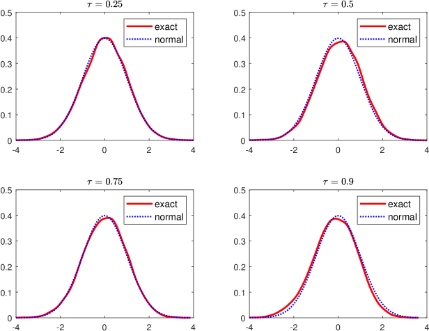
Figure 1: Finite sample exact distribution of the studentized location effect statistic when $\gamma=0.25$, $\sigma_{X}^{2}=1$, and $n=1000.$

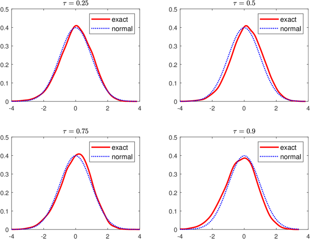
Figure 2: Finite sample exact distribution of the studentized location effect statistic when $\gamma=0.75$, $\sigma_{X}^{2}=1$, and $n=1000.$

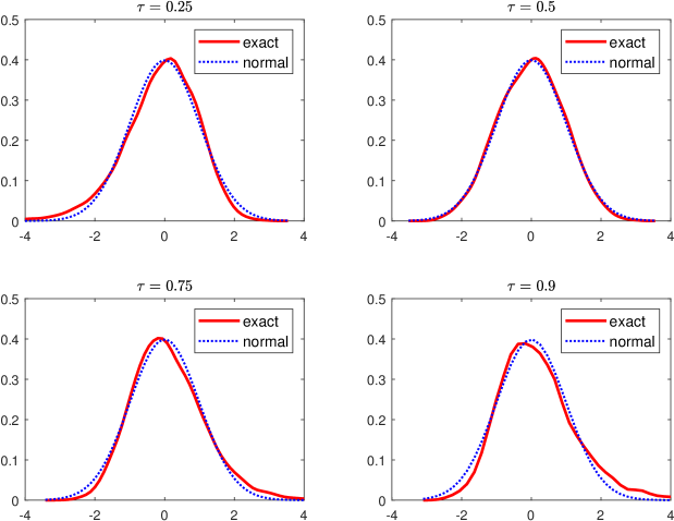
Figure 3: Finite sample exact distribution of the studentized scale effect statistic when $\gamma=0.25$, $\sigma_{X}^{2}=1$, and $n=1000.$

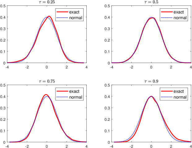
Figure 4: Finite sample exact distribution of the studentized scale effect statistic when $\gamma=0.75$, $\sigma_{X}^{2}=1$, and $n=1000.$

Table 2 reports the empirical coverage of 95% confidence intervals for the location and scale effects. The empirical coverage is close to the nominal coverage in all cases. This is consistent with Figures 1–4. We may then conclude that the normal approximation can be reliably used for inference on the location and scale effects.

Table 2: Empirical coverage of 95% confidence intervals for the location and scale effects when $\sigma_{X}^{2}=1.$

	$\gamma$	$\tau=0.1$	$\tau=0.25$	$\tau=0.50$	$\tau=0.75$	$\tau=0.90$
	$n=500$
Location	${0.25}$	$0.946$	$0.950$	$0.951$	$0.950$	$0.947$
	${0.5}$	$0.942$	$0.952$	$0.950$	$0.953$	$0.938$
	${0.75}$	$0.940$	$0.954$	$0.952$	$0.956$	$0.937$
	${1}$	$0.937$	$0.957$	$0.950$	$0.957$	$0.935$
Scale	${0.25}$	$0.900$	$0.921$	$0.973$	$0.916$	$0.902$
	${0.5}$	$0.930$	$0.943$	$0.957$	$0.939$	$0.928$
	${0.75}$	$0.937$	$0.950$	$0.954$	$0.946$	$0.933$
	${1}$	$0.939$	$0.952$	$0.951$	$0.945$	$0.933$
	$n=1000$
Location	$0.25$	$0.948$	$0.951$	$0.951$	$0.954$	$0.945$
	$0.5$	$0.946$	$0.950$	$0.952$	$0.957$	$0.943$
	$0.75$	$0.945$	$0.952$	$0.953$	$0.957$	$0.940$
	$1$	$0.941$	$0.952$	$0.952$	$0.958$	$0.942$
Scale	$0.25$	$0.922$	$0.939$	$0.965$	$0.940$	$0.921$
	$0.5$	$0.938$	$0.949$	$0.955$	$0.950$	$0.933$
	$0.75$	$0.942$	$0.951$	$0.952$	$0.952$	$0.938$
	$1$	$0.939$	$0.952$	$0.950$	$0.953$	$0.940$

5.3 Power of the t-test of a zero scale effect

To investigate the power of the t-test proposed in Corollary 3, we simulate the following model:

$$Y=\lambda+X\gamma+U,$$

where

$$\begin{pmatrix}X\\ U\end{pmatrix}\sim N\left(\begin{pmatrix}1\\ 0\end{pmatrix},\begin{pmatrix}1&0\\ 0&1\end{pmatrix}\right).$$

Here we set $\lambda=0,$ $\mu_{X}=1$ and $\dot{s}(0)=-1$. When $\gamma=0$, $X$ is excluded from the outcome equation and thus the scale effect is 0. The null hypothesis of a zero scale effect corresponds to the case that $\gamma=0$. The power of the test is obtained by varying $\gamma$ around 0 in a grid from $-0.4$ to $0.4$ with an increment of $0.01$.

Figure 5 graphs the size-adjusted power of the t-test for different quantile levels when $n=500$ and when $n=1000$. The power is calculated using the probit specification, namely $F_{Y|X}(Q_{\tau}[Y]|X)=\bm{\Phi}(X\alpha_{\tau}+\beta_{\tau})$. The size adjustment is based on the empirical critical value such that the test rejects the null 5% of the time. Figure 5 shows that the power increases as $\gamma$ deviates more from its null value of zero, and that for a given nonzero value of $\gamma,$ the power increases with the sample size. Results not reported here show that the test has a quite accurate size in that the empirical rejection probability under the null is close to 5%, the nominal level of the test.

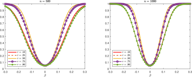
Figure 5: Size-adjusted power of the t-test for a zero scale effect.

6 Empirical application

In this section, we consider two applications: education and wages, and smoking and birth weights.

6.1 Education and wages

Our first application is based on a household labor survey from Wooldridge (2002) that can be accessed online for replication. The idea is to evaluate the effects of education on the quantile of the unconditional distribution of log wages. In this application, $Y=lwage,$ which is log hourly wage, and $X=educ$, which is years of education is our target variable. The controls are: $W=[exper\ tenure\ nonwhite\ female]$, where $exper$ is years of working experience, $tenure$ is years with current employer, $nonwhite$ is a dummy that equals 1 if the individual is non-white, and $female$ is a dummy that equals 1 if the individual is female. We assume that Assumption 2 holds for this choice of $W.$

While the main goal is to study the scale effect, we also present results for the location effect. We set $\dot{\ell}(0)=1$ and $\dot{s}(0)=-1$. Note that when $\dot{s}(0)=-1,$ the estimated effects we present below are the unconditional scale effects when the variance of the covariate is reduced by a small amount. For the mean of years of education $\mu_{X}$, we let $\mu_{X}=12.29$ based on the Barro-Lee Data on Educational Attainment. We set $\mu=\mu_{X}=12.29$ to study the location and scale effects. In a similar fashion to the Monte Carlo analysis, we consider $\tau\in\{0.10,0.25,0.50,0.75,0.90\}$. The sample size for the household labor survey is $n=526$, which is comparable to $n=500$ in the simulation exercises. We compute the standard errors using the approximation in (21).

Table 3: Effects of location-scale shifts in education on the unconditional quantiles of log-wage.

		$\tau=0.10$	$\tau=0.25$	$\tau=0.50$	$\tau=0.75$	$\tau=0.90$
Location (probit)	Estimate	0.039	0.062	0.101	0.101	0.118
		(0.008)	(0.011)	(0.015)	(0.016)	(0.021)
	$95\%\ CI_{L}$	0.025	0.041	0.072	0.069	0.076
	$95\%\ CI_{U}$	0.054	0.083	0.129	0.132	0.160
Location (logit)	Estimate	0.038	0.065	0.103	0.100	0.120
		(0.007)	(0.010)	(0.015)	(0.016)	(0.021)
	$95\%\ CI_{L}$	0.024	0.044	0.074	0.069	0.080
	$95\%\ CI_{U}$	0.053	0.085	0.131	0.132	0.160
Scale (probit)	Estimate	0.045	0.029	-0.025	-0.103	-0.203
		(0.014)	(0.011)	(0.013)	(0.028)	(0.065)
	$95\%\ CI_{L}$	0.018	0.007	-0.051	-0.158	-0.330
	$95\%\ CI_{U}$	0.071	0.052	0.001	-0.049	-0.077
Scale (logit)	Estimate	0.045	0.034	-0.024	-0.110	-0.227
		(0.014)	(0.012)	(0.014)	(0.029)	(0.066)
	$95\%\ CI_{L}$	0.017	0.011	-0.051	-0.167	-0.356
	$95\%\ CI_{U}$	0.072	0.058	0.002	-0.053	-0.099

Notes: standard errors are in parentheses.

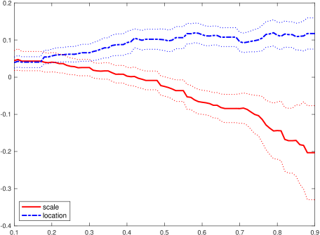
Figure 6: Point and interval estimates of the location and scale effects of education on the unconditional quantiles of log-wage based on the probit specification: $\Pi_{\tau,L}$ (dashed blue) and $\Pi_{\tau,S}$ (solid red).

The most interesting results in Table 3 appear in the unconditional scale effects. As discussed in Section 2.4, the scale effects can be interpreted as percentage changes of the unconditional quantiles. Consider the scale effect for $\tau=0.10$. Both the probit and logit specifications suggest an effect of about .045. Then, using the quantile-standard deviation elasticity, a $1\%$ decrease in the standard deviation of education would produce a positive effect of $.045\%$ on the unconditional quantile at the quantile level $\tau=0.10$. Given that the sample standard deviation of $educ$ is $2.77$, the $1\%$ decrease is approximately a change in the standard deviation from $2.77$ to $2.74$. Consider now the scale effect for $\tau=0.50$. In this case, both probit and logit specifications provide a statistically insignificant effect (at the $5\%$ level). Confront this with the results of Example 7 where in the linear model $Y=\lambda+X\gamma+U$, the scale effect $\Pi_{0.50,S}=0$ if both $X$ and $U$ are symmetrically distributed around 0. Thus, $\hat{\Pi}_{0.50,S}\approx 0$ is consistent with a linear model with symmetrically distributed $X$ and $U.$ Finally, consider the scale effect for $\tau=0.90$, again using both probit and logit specifications. In this case, the effects are negative, suggesting a $1\%$ decrease in the standard deviation would reduce the upper $\tau=0.90$ quantile by $.20\%$ (probit) and $.23\%$ (logit). Overall this analysis shows that the scale effects are monotonically decreasing in $\tau$. This can be seen in Figure 6 that plots, for a finer grid of $\tau$, the probit estimates for both the location (dashed blue) and scale (solid red) effects.

How can this be interpreted? The location effects suggest that the marginal contribution of one more year of education benefits more the upper parts of the unconditional distribution of wages. The scale effects suggest the contrary. Reducing the overall dispersion of education would increase the lower quantile wages, but reduce the upper ones.

Table 4: Effects of location-scale shifts in education on the unconditional quantiles of log-wage.

		$\tau=0.10$	$\tau=0.25$	$\tau=0.50$	$\tau=0.75$	$\tau=0.90$
Location (probit)	Estimate	0.039	0.062	0.101	0.101	0.118
		(0.008)	(0.011)	(0.015)	(0.016)	(0.021)
	$95\%\ CI_{L}$	0.025	0.041	0.072	0.069	0.076
	$95\%\ CI_{U}$	0.054	0.083	0.129	0.132	0.160
Location (logit)	Estimate	0.038	0.065	0.103	0.100	0.120
		(0.007)	(0.010)	(0.015)	(0.016)	(0.021)
	$95\%\ CI_{L}$	0.024	0.044	0.074	0.069	0.080
	$95\%\ CI_{U}$	0.053	0.085	0.131	0.132	0.160
Scale (probit)	Estimate	0.045	0.029	-0.025	-0.103	-0.203
		(0.014)	(0.011)	(0.013)	(0.028)	(0.065)
	$95\%\ CI_{L}$	0.018	0.007	-0.051	-0.158	-0.330
	$95\%\ CI_{U}$	0.071	0.052	0.001	-0.049	-0.077
Scale (logit)	Estimate	0.045	0.034	-0.024	-0.110	-0.227
		(0.014)	(0.012)	(0.014)	(0.029)	(0.066)
	$95\%\ CI_{L}$	0.017	0.011	-0.051	-0.167	-0.356
	$95\%\ CI_{U}$	0.072	0.058	0.002	-0.053	-0.099

Notes: standard errors are in parentheses.

6.2 Smoking and birth weight

This second application considers the relationship between smoking during pregnancy and the child’s birth weight. This was previously studied by Abrevaya (2001), Koenker and Hallock (2001), Rothe (2010), and Chernozhukov and Fernández-Val (2011). We use the natality data from the National Vital Statistics System for the year 2018. The outcome variable is birth weight in grams, while the target variable is the average number of cigarettes smoked daily during pregnancy. We focus on the sample of mothers who are smokers. The sample consists of 219,667 observations.

For this model $Y$ is birth weight in grams and $X$ is the mother’s reported average number of cigarettes smoked per day during pregnancy. We use the same covariates as Abrevaya (2001): $(i)$ a dummy for whether the mother is black; $(ii)$ a dummy for marital status; $(iii)$ age and age squared; $(iv)$ a set of dummies for education attainment: high school graduate, some college, and college graduate; $(v)$ weight gain during pregnancy, $(vi)$ a set of dummies for prenatal visit: visit during the second trimester, visit during the third trimester, and no visit at all; and $(vii)$ a dummy for the sex of the child.

For this application, we set $\mu=0$, $l(\delta)\equiv 0$, and $s(\delta)=1/\left(1+\delta\right)$, so that according to (2), counterfactual cigarette consumption is now $X_{\delta}=X/(1+\delta)$, which has a smaller mean and variance than $X.$ Note, again, that $\dot{s}(0)=-1$. To motivate such a counterfactual policy, we can think of a tax on the price of cigarettes, which induces the consumer to reduce cigarette consumption from $X$ to $X/(1+\delta)$. .

Table 5 and Figure 7 show the results. The effects are positive and monotonically increasing across quantiles. This means that the marginal impact on the birth weight of a tax on cigarettes is positive. The effects are stronger for upper quantiles of the distribution of birth weight. In order to interpret the magnitudes, we use the quantile-standard deviation elasticity. According to (10), the elasticity can be calculated as $\mathcal{E}_{\tau,\delta=0}=-\Pi_{\tau,S}/Q_{\tau}[Y]$ as $\dot{s}\left(0\right)=-1.$ For example, for $\tau=0.50$, $\mathcal{E}_{0.50,\delta=0}=-0.0128$. This means that a $1\%$ decrease in the standard deviation of the consumption of cigarettes increases the median birth weight by $0.0128\%$.

Table 5: Effects of a negative location-scale shift in smoking ($X_{\delta}=X/\left(1+\delta)\right)$ on the unconditional quantiles of birth weight.

		$\tau=0.10$	$\tau=0.25$	$\tau=0.50$	$\tau=0.75$	$\tau=0.90$
Scale (probit)	Estimate	26.562	35.412	39.096	41.316	46.249
		(2.784)	(1.870)	(1.708)	(2.024)	(2.834
	$95\%\ CI_{L}$	21.106	31.746	35.749	37.349	40.694
	$95\%\ CI_{U}$	32.018	39.078	42.443	45.282	51.803
Scale (logit)	Estimate	25.242	34.412	40.038	44.232	50.077
		(2.722)	(1.848)	(1.711)	(1.984)	(2.695)
	$95\%\ CI_{L}$	19.908	30.790	36.684	40.343	44.795
	$95\%\ CI_{U}$	30.577	38.034	43.392	48.122	55.360

Notes: standard errors are in parentheses.

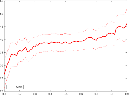
Figure 7: Point and interval estimates of the location-scale effects of smoking on the unconditional quantiles of birth weight based on the probit specification.

7 Conclusion

This paper has provided a general procedure to analyze the distributional impact of changes in covariates on an outcome variable. The standard unconditional quantile regression analysis focuses on a particular impact coming from a location shift. We have provided a framework to study the unconditional policy effects generated by a smooth and invertible intervention of one or more target variables, allowing them to be possibly endogeneous. We focus particularly on a location-scale shift and show how to additively decompose the total effect into a location effect and a scale effect. They can be analyzed and estimated separately. Additionally, we consider the case of simultaneous changes in different covariates. We show how this can be obtained from the usual vector-valued unconditional quantile regressions.

Appendix

A.1 Proof of Theorem 1

Part (i). To obtain the joint density of $\left(X_{\delta},W\right)$, we note that

$$F_{X_{\delta},W}(x,w)=\Pr(X_{\delta}\leq x,W\leq w)=\Pr(X\leq x^{\delta},W\leq w)=F_{X,W}(x^{\delta},w),$$

and so

$$f_{X_{\delta},W}(x,w)=\frac{\partial x^{\delta}}{\partial x}\cdot f_{X,W}(x^{\delta},w)=J(x^{\delta};\delta)f_{X,W}(x^{\delta},w).$$

Evaluated at $\delta=0,$ $J\left(x^{\delta};\delta\right)$ is $1$ and $f_{X_{\delta},W}(x,w)$ is $f_{X,W}(x,w)$. Given this, we expand $f_{X_{\delta},W}(x,w)-f_{X,W}(x,w)$ around $\delta=0$, which is possible under Assumptions 1(i) and (iii.a). First, we observe that

$$\frac{\partial J(x^{\delta};\delta)}{\partial x^{\delta}} =\frac{\partial}{\partial x^{\delta}}\frac{\partial x^{\delta}}{\partial x}=\frac{\partial}{\partial x}\frac{\partial x^{\delta}}{\partial x^{\delta}}=0,$$

$$\frac{\partial J(x^{\delta};\delta)}{\partial\delta}\bigg{|}_{\delta=0} =\frac{\partial}{\partial\delta}\frac{\partial x^{\delta}}{\partial x}\bigg{|}_{\delta=0}=\frac{\partial}{\partial x}\frac{\partial x^{\delta}}{\partial\delta}\bigg{|}_{\delta=0}=-\frac{\partial\kappa\left(x\right)}{\partial x},$$

where the last line follows from the fact that

$$\kappa\left(x\right):=\frac{\partial\mathcal{G}(x;\delta)}{\partial\delta}\bigg{|}_{\delta=0}=-\frac{\partial x^{\delta}}{\partial\delta}\bigg{|}_{\delta=0}.$$

Differentiating both sides of $\mathcal{G}\left(x^{\delta};\delta\right)=x$ with respect to $\delta,$ we obtain that

$$\frac{\partial x^{\delta}}{\partial\delta}=-\left(\frac{\partial\mathcal{G}\left(x^{\delta};\delta\right)}{\partial x^{\delta}}\right)^{-1}\frac{\partial\mathcal{G}\left(x^{\delta};\delta\right)}{\partial\delta}$$

and so

$$-\frac{\partial x^{\delta}}{\partial\delta}\bigg{|}_{\delta=0}=\left(\frac{\partial\mathcal{G}\left(x;0\right)}{\partial x}\right)^{-1}\frac{\partial\mathcal{G}\left(x;\delta\right)}{\partial\delta}\bigg{|}_{\delta=0}=\frac{\partial\mathcal{G}\left(x;\delta\right)}{\partial\delta}\bigg{|}_{\delta=0}:=\kappa(x),$$

where we have used $\mathcal{G}\left(x;0\right)=x.$ Now we have

$$f_{X_{\delta},W}(x,w)-f_{X,W}(x,w)$$

$$=J(x^{\delta};\delta)f_{X,W}(x^{\delta},w)-f_{X,W}(x,w)$$

$$=\delta\left[\frac{\partial J\left(x^{\delta};\delta\right)}{\partial x^{\delta}}\frac{\partial x^{\delta}}{\partial\delta}+\frac{\partial J\left(x^{\delta};\delta\right)}{\partial\delta}\right]\bigg{|}_{\delta=0}f_{X,W}(x,w)$$

$$+\delta J\left(x;0\right)\frac{\partial f_{X,W}(x,w)}{\partial x}\frac{\partial x^{\delta}}{\partial\delta}\bigg{|}_{\delta=0}+\delta R_{1}(x,w,\delta)$$

$$=\delta\frac{\partial J\left(x^{\delta};\delta\right)}{\partial\delta}\bigg{|}_{\delta=0}f_{X,W}(x,w)+\delta J\left(x;0\right)\frac{\partial f_{X,W}(x,w)}{\partial x}\frac{\partial x^{\delta}}{\partial\delta}\bigg{|}_{\delta=0}+\delta R_{1}(x,w,\delta)$$

$$=\delta\left[-\frac{\partial\kappa\left(x\right)}{\partial x}f_{X,W}(x,w)-\frac{\partial f_{X,W}(x,w)}{\partial x}\kappa\left(x\right)\right]+\delta R_{1}(x,w,\delta)$$

$$=-\delta\frac{\partial}{\partial x}\left[\kappa\left(x\right)f_{X,W}(x,w)\right]+\delta R_{1}(x,w,\delta),$$

where, for $\tilde{\delta}(x,w)$ between $0$ and $\delta$,

$$R_{1}(x,w,\delta)=\left\{\frac{\partial\left[J\left(x^{\delta};\delta\right)f_{X,W}(x^{\delta},w)\right]}{\partial\delta}\bigg{|}_{\delta=\tilde{\delta}(x,w)}-\frac{\partial\left[J\left(x^{\delta};\delta\right)f_{X,W}(x^{\delta},w)\right]}{\partial\delta}\bigg{|}_{\delta=0}\right\}.$$ (A.1)

By the continuity of the derivative of $J\left(x^{\delta};\delta\right)f_{X,W}(x^{\delta},w)$ with respect to $\delta$, we have $R_{1}(x,w,\delta)=o(1)$ for each $\left(x,w\right)$ as $\delta\rightarrow 0.$

Part (ii). Consider first the counterfactual distribution $F_{Y_{\delta}}$:

$$F_{Y_{\delta}}(y)=\int_{\mathcal{W}}\int_{\mathcal{X}}\int_{\mathcal{U}}\mathds{1}\left\{h(x,w,u)\leq y\right\}f_{U|X_{\delta},W}(u|x,w)f_{X_{\delta},W}(x,w)dudxdw,$$

where for simplicity we have assumed that the support of $X$ conditional on any $W=w$ does not depend on $w$ and we have denoted the support by $\mathcal{X}$. By Assumption 1(ii), $f_{U|X_{\delta},W}(u|x,w)=f_{U|X,W}(u|x^{\delta},w)$. So we can write

$$F_{Y_{\delta}}(y)$$

$$=\int_{\mathcal{W}}\int_{\mathcal{X}}\int_{\mathcal{U}}\mathds{1}\left\{h(x,w,u)\leq y\right\}f_{U|X_{\delta},W}(u|x,w)f_{X_{\delta},W}(x,w)dudxdw$$

$$=\int_{\mathcal{W}}\int_{\mathcal{X}}\int_{\mathcal{U}}\mathds{1}\left\{h(x,w,u)\leq y\right\}f_{U|X,W}(u|x^{\delta},w)f_{X_{\delta},W}(x,w)dudxdw$$

$$=\underbrace{\int_{\mathcal{W}}\int_{\mathcal{X}}\int_{\mathcal{U}}\mathds{1}\left\{h(x,w,u)\leq y\right\}f_{U|X,W}(u|x,w)f_{X,W}(x,w)dudxdw}_{=F_{Y}(y)}$$

$$+\int_{\mathcal{W}}\int_{\mathcal{X}}\int_{\mathcal{U}}\mathds{1}\left\{h(x,w,u)\leq y\right\}f_{U|X,W}(u|x,w)\left[f_{X_{\delta},W}(x,w)-f_{X,W}(x,w)\right]dudxdw$$

$$+\int_{\mathcal{W}}\int_{\mathcal{X}}\int_{\mathcal{U}}\mathds{1}\left\{h(x,w,u)\leq y\right\}\left[f_{U|X,W}(u|x^{\delta},w)-f_{U|X,W}(u|x,w)\right]f_{X_{\delta},W}(x,w)dudxdw.$$

Hence, we have

$$\frac{F_{Y_{\delta}}(y)-F_{Y}(y)}{\delta}:=G_{1,\delta}\left(y\right)+G_{2,\delta}\left(y\right),$$

where

$$G_{1,\delta}\left(y\right) =\int_{\mathcal{W}}\int_{\mathcal{X}}\int_{\mathcal{U}}\mathds{1}\left\{h(x,w,u)\leq y\right\}f_{U|X,W}(u|x,w)\frac{1}{\delta}\left[f_{X_{\delta},W}(x,w)-f_{X,W}(x,w)\right]dudxdw$$

$$=\int_{\mathcal{W}}\int_{\mathcal{X}}F_{Y|X,W}(y|x,w)\frac{1}{\delta}\left[f_{X_{\delta},W}(x,w)-f_{X,W}(x,w)\right]dxdw,$$ (A.2)

and

$$G_{2,\delta}\left(y\right) =\int_{\mathcal{W}}\int_{\mathcal{X}}\int_{\mathcal{U}}\mathds{1}\left\{h(x,w,u)\leq y\right\}$$

$$\times\frac{1}{\delta}\left[f_{U|X,W}(u|x^{\delta},w)-f_{U|X,W}(u|x,w)\right]f_{X_{\delta},W}(x,w)dudxdw.$$ (A.3)

We first consider the term $G_{1,\delta}\left(y\right).$ Using Part (i) and Assumption 1(iv), we have

$$G_{1,\delta}\left(y\right) =-\int_{\mathcal{W}}\int_{\mathcal{X}}F_{Y|X,W}\left(y|x,w\right)\frac{\partial\left[\kappa\left(x\right)f_{X,W}(x,w)\right]}{\partial x}$$

$$+\int_{\mathcal{W}}\int_{\mathcal{X}}F_{Y|X,W}(y|x,w)R_{1}(x,w,\delta)dxdw$$

$$=\int_{\mathcal{W}}\int_{\mathcal{X}}\frac{\partial F_{Y|X,W}(y|x,w)}{\partial x}\kappa\left(x\right)f_{X,W}(x,w)dxdw$$

$$+\int_{\mathcal{W}}\int_{\mathcal{X}}F_{Y|X,W}(y|x,w)R_{1}(x,w,\delta)dxdw,$$

where the second equality follows from integration by parts. Under Assumption 1(iii.a), we can use the dominated convergence theorem to obtain

$$\lim_{\delta\rightarrow 0}\sup_{y\in\mathcal{Y}}\bigg{|}\int_{\mathcal{W}}\int_{\mathcal{X}}F_{Y|X,W}(y|x,w)R_{1}(x,w,\delta)dxdw\bigg{|}=0.$$

Thus, we have that $G_{1,\delta}\left(y\right)$ converges to $G_{1,0}\left(y\right)$, given by

$$G_{1,0}\left(y\right):=\int_{\mathcal{W}}\int_{\mathcal{X}}\frac{\partial F_{Y|X,W}(y|x,w)}{\partial x^{\prime}}\kappa\left(x\right)f_{X,W}(x,w)dxdw$$

uniformly in $y\in\mathcal{Y}$, as $\delta\rightarrow 0$.

Next, we consider $G_{2,\delta}\left(y\right).$ Using Assumption 1(iii.b), we have

$$\left[f_{U|X,W}(u|x^{\delta},w)-f_{U|X,W}(u|x,w)\right]f_{X,W}(x^{\delta},w)$$

$$=\frac{\partial f_{U|X,W}(u|x^{\delta},w)}{\partial x^{\delta\prime}}f_{X,W}(x^{\delta},w)\frac{\partial x^{\delta}}{\partial\delta}\bigg{|}_{\delta=0}\cdot\delta+\delta R_{2}(u,x,w,\delta)$$

$$=-\frac{\partial f_{U|X,W}(u|x,w)}{\partial x^{\prime}}f_{X,W}(x,w)\kappa\left(x\right)\delta+\delta R_{2}(u,x,w,\delta),$$

where

$$R_{2}(u,x,w,\delta)$$

$$=\frac{\partial\left[f_{U|X,W}(u|x^{\delta},w)f_{X,W}(x^{\delta},w)\right]}{\partial\delta}\bigg{|}_{\delta=\tilde{\delta}(u,x,w)}-\frac{\partial\left[f_{U|X,W}(u|x^{\delta},w)f_{X,W}(x^{\delta},w)\right]}{\partial\delta}\bigg{|}_{\delta=0}$$

$$-\left[f_{U|X,W}(u|x,w)\frac{\partial f_{X,W}(x^{\delta},w)}{\partial\delta}\bigg{|}_{\delta=\tilde{\delta}(u,x,w)}-f_{U|X,W}(u|x,w)\frac{\partial f_{X,W}(x^{\delta},w)}{\partial\delta}\bigg{|}_{\delta=0}\right].$$

Note that in the above, the transpose on $x$ is not relevant but we keep it so that the same lines of arguments can be used for proving Theorem S.1. Hence

$$G_{2,\delta}\left(y\right) =-\int_{\mathcal{W}}\int_{\mathcal{X}}\int_{\mathcal{U}}\mathds{1}\left\{h(x,w,u)\leq y\right\}\frac{\partial f_{U|X,W}(u|x,w)}{\partial x^{\prime}}f_{X,W}(x,w)\kappa\left(x\right)dudxdw$$

$$+\int_{\mathcal{W}}\int_{\mathcal{X}}\int_{\mathcal{U}}\mathds{1}\left\{h(x,w,u)\leq y\right\}R_{2}(u,x,w,\delta)dudxdw.$$

Under Assumption 1(iii.b), we can invoke the dominated convergence theorem to get

$$\lim_{\delta\rightarrow 0}\sup_{y\in\mathcal{Y}}\left|\int_{\mathcal{W}}\int_{\mathcal{X}}\int_{\mathcal{U}}\mathds{1}\left\{h(x,w,u)\leq y\right\}R_{2}(u,x,w,\delta)dudxdw\right|=0.$$

Hence, uniformly in $y\in\mathcal{Y}$, as $\delta\rightarrow 0$, $G_{2,\delta}\left(y\right)$ converges to

$$G_{2,0}\left(y\right) =-\int_{\mathcal{W}}\int_{\mathcal{X}}\int_{\mathcal{U}}\mathds{1}\left\{h(x,w,u)\leq y\right\}\frac{\partial f_{U|X,W}(u|x,w)}{\partial x^{\prime}}\kappa\left(x\right)f_{X,W}(x,w)dudxdw$$

$$=-\int_{\mathcal{W}}\int_{\mathcal{X}}\int_{\mathcal{U}}\mathds{1}\left\{h(x,w,u)\leq y\right\}\frac{\partial\ln f_{U|X,W}(u|x,w)}{\partial x^{\prime}}\kappa\left(x\right)f_{U|X,W}(u|x,w)f_{X,W}(x,w)dudxdw$$

$$=-E\left[\mathds{1}\left\{h(X,W,U)\leq y\right\}\frac{\partial\ln f_{U|X,W}(U|X,W)}{\partial X^{\prime}}\kappa\left(X\right)\right].$$

Combining the above results yields

$$\frac{F_{Y_{\delta}}(y)-F_{Y}\left(y\right)}{\delta}$$

$$\rightarrow G_{10}\left(y\right)+G_{20}(y)$$

$$=E\left[\left(\frac{\partial F_{Y|X,W}(y|X,W)}{\partial X^{\prime}}-\mathds{1}\left\{h(X,W,U)\leq y\right\}\frac{\partial\ln f_{U|X,W}(U|X,W)}{\partial X^{\prime}}\right)\kappa\left(X\right)\right]$$

$$:=G\left(y\right)$$

uniformly over $y\in\mathcal{Y}$ as $\delta\rightarrow 0.$

Part (iii). Note that $\psi\left(y,\tau,F_{Y}\right)$ is the influence function of the quantile functional. Using Part (ii) and Assumption 1(v), we have

$$\Pi_{\tau}=\int_{\mathcal{Y}}\psi\left(y,\tau,F_{Y}\right)dG\left(y\right)=\int_{\mathcal{Y}}\psi\left(y,\tau,F_{Y}\right)dG_{1,0}\left(y\right)+\int_{\mathcal{Y}}\psi\left(y,\tau,F_{Y}\right)dG_{2,0}\left(y\right)$$

by Lemma 21.3 in van der Vaart (1998). Now

$$\int_{\mathcal{Y}}\psi\left(y,\tau,F_{Y}\right)dG_{1,0}\left(y\right) =\int_{\mathcal{Y}}\psi\left(y,\tau,F_{Y}\right)dG_{1,0}\left(y\right)$$

$$=\int_{\mathcal{W}}\int_{\mathcal{X}}\left[\int_{\mathcal{Y}}\psi\left(y,\tau,F_{Y}\right)\frac{\partial f_{Y|X,W}(y|x,w)}{\partial x^{\prime}}dy\right]\kappa\left(x\right)f_{X,W}(x,w)dxdw$$

$$=\int_{\mathcal{W}}\int_{\mathcal{X}}\frac{\partial}{\partial x^{\prime}}\left[\int_{\mathcal{Y}}\psi\left(y,\tau,F_{Y}\right)f_{Y|X,W}(y|x,w)dy\right]\kappa\left(x\right)f_{X,W}(x,w)dxdw$$

$$=\int_{\mathcal{W}}\int_{\mathcal{X}}\frac{\partial E\left[\psi\left(Y,\tau,F_{Y}\right)|X=x,W=w\right]}{\partial x^{\prime}}\kappa\left(x\right)f_{X,W}(x,w)dxdw$$

and

$$\int_{\mathcal{Y}}\psi\left(y,\tau,F_{Y}\right)dG_{2,0}\left(y\right)$$

$$=-\int_{\mathcal{W}}\int_{\mathcal{X}}\int_{\mathcal{U}}\left[\int_{\mathcal{Y}}\psi\left(y,\tau,F_{Y}\right)d\mathds{1}\left\{h(x,w,u)\leq y\right\}\right]\frac{\partial\ln f_{U|X,W}(u|x,w)}{\partial x^{\prime}}\kappa\left(x\right)$$

$$\times f_{U|X,W}(u|x,w)f_{X,W}(x,w)dudxdw$$

$$=-\int_{\mathcal{W}}\int_{\mathcal{X}}\int_{\mathcal{U}}\psi\left(h(x,w,u),\tau,F_{Y}\right)\frac{\partial\ln f_{U|X,W}(u|x,w)}{\partial x^{\prime}}\kappa\left(x\right)$$

$$\times f_{U|X,W}(u|x,w)f_{X,W}(x,w)dudxdw.$$

Therefore,

$$\Pi_{\tau} =\int_{\mathcal{W}}\int_{\mathcal{X}}\frac{\partial E\left[\psi\left(y,\tau,F_{Y}\right)|X=x,W=w\right]}{\partial x^{\prime}}\kappa\left(x\right)f_{X,W}(x,w)dxdwdy$$

$$-\int_{\mathcal{W}}\int_{\mathcal{X}}\int_{\mathcal{U}}\psi\left(h(x,w,u),\tau,F_{Y}\right)\frac{\partial\ln f_{U|X,W}(u|x,w)}{\partial x^{\prime}}\kappa\left(x\right)$$

$$\times f_{U|X,W}(u|x,w)f_{X,W}(x,w)dudxdw$$

$$=A_{\tau}-B_{\tau}.$$

A.2 Proof of Lemma 1

The main complication in this lemma is that the dependent variable is $\mathds{1}\left\{Y_{i}\leq\hat{q}_{\tau}\right\}$. This means that the preliminary estimator $\hat{q}_{\tau}$ might affect the asymptotic distribution of $\hat{\alpha}_{\tau}$ and $\hat{\beta}_{\tau}$.

As mentioned in the main text, under Assumption 4,

$$\hat{q}_{\tau}-Q_{\tau}[Y]=\frac{1}{n}\sum_{i=1}^{n}\frac{\tau-\mathds{1}\left\{Y_{i}\leq Q_{\tau}[Y]\right\}}{f_{Y}(Q_{\tau}[Y])}+o_{p}(n^{-1/2})=\frac{1}{n}\sum_{i=1}^{n}\psi(Y_{i},\tau,F_{Y})+o_{p}(n^{-1/2}).$$

Recall that

$$\hat{\theta}_{\tau}=\arg\max_{\theta\in\Theta}\sum_{i=1}^{n}\bigg{\{}\mathds{1}\left\{Y_{i}\leq\hat{q}_{\tau}\right\}\log\left[G(Z_{i}^{\prime}\theta)\right]+\mathds{1}\left\{Y_{i}>\hat{q}_{\tau}\right\}\log\left[1-G(Z_{i}^{\prime}\theta)\right]\bigg{\}}.$$

Let $s_{i}(\theta;\hat{q}_{\tau})$ denote the score for observation $i$. Then, under Assumption 5(i), we have

$$\frac{1}{n}\sum_{i=1}^{n}s_{i}(\hat{\theta}_{\tau};\hat{q}_{\tau})=0.$$

Taking a mean-value expansion (element-by-element), we obtain

$$\underbrace{\frac{1}{n}\sum_{i=1}^{n}s_{i}(\hat{\theta}_{\tau};\hat{q}_{\tau})}_{=0}=\frac{1}{n}\sum_{i=1}^{n}s_{i}(\theta_{\tau};\hat{q}_{\tau})+\frac{1}{n}\sum_{i=1}^{n}H_{i}(\tilde{\theta}_{\tau};\hat{q}_{\tau})\left(\hat{\theta}_{\tau}-\theta_{\tau}\right),$$

where $\tilde{\theta}_{\tau}$ is between $\theta_{\tau}$ and $\hat{\theta}_{\tau}$ and can be different for different rows of $H_{i}.$ Under the assumption of the uniform law of large numbers for the Hessian (i.e., Assumption 5(ii)), we obtain

$$\frac{1}{n}\sum_{i=1}^{n}H_{i}(\tilde{\theta}_{\tau},\hat{q}_{\tau})\overset{p}{\rightarrow}E[H_{i}(\theta_{\tau};Q_{\tau}[Y])]=:H.$$

We have then

$$0=\frac{1}{n}\sum_{i=1}^{n}s_{i}(\theta_{\tau};\hat{q}_{\tau})+H\left(\hat{\theta}_{\tau}-\theta_{\tau}\right)+o_{p}\left(\left\|\hat{\theta}_{\tau}-\theta_{\tau}\right\|\right).$$ (A.4)

Now, we use the stochastic equicontinuity in Assumption 5(iii):

$$\frac{1}{n}\sum_{i=1}^{n}\left(s_{i}(\theta_{\tau};\hat{q}_{\tau})-E\left[s_{i}(\theta_{\tau};q)\right]|_{q=\hat{q}_{\tau}}\right)=\frac{1}{n}\sum_{i=1}^{n}s_{i}(\theta_{\tau};Q_{\tau}[Y])+o_{p}(n^{-1/2}).$$

Here we have used that $E[s_{i}(\theta_{\tau};Q_{\tau}[Y])]=0$: the score evaluated at the true quantile has expected value 0. Plugging this back into (A.4), we obtain

$$0=E\left[s_{i}(\theta_{\tau};q)\right]|_{q=\hat{q}_{\tau}}+\frac{1}{n}\sum_{i=1}^{n}s_{i}(\theta_{\tau};Q_{\tau}[Y])+H\left(\hat{\theta}_{\tau}-\theta_{\tau}\right)+o_{p}\left(\left\|\hat{\theta}_{\tau}-\theta_{\tau}\right\|\right).$$ (A.5)

Here $E\left[s_{i}(\theta_{\tau};q)\right]|_{q=\hat{q}_{\tau}}$ is random because we first compute the expectation $E\left[s_{i}(\theta_{\tau};q)\right]$ for a fixed $q$ and then replace $q$ by $\hat{q}_{\tau}$, which is random. To show that $E\left[s_{i}(\theta_{\tau};q)\right]|_{q=\hat{q}_{\tau}}$ is $O_{p}(n^{-1/2})$, we observe that (see equation 15.18 in Wooldridge (2002))

$$s_{i}(\theta;q)=\dfrac{g(Z_{i}^{\prime}\theta)Z_{i}\left[\mathds{1}\left\{Y_{i}\leq q\right\}-G\left(Z_{i}^{\prime}\theta\right)\right]}{G\left(Z_{i}^{\prime}\theta\right)\left[1-G\left(Z_{i}^{\prime}\theta\right)\right]}.$$ (A.6)

Therefore, using the law of iterated expectations, we obtain

$$E\left[s_{i}(\theta;q)\right]=E\left[\dfrac{g(Z_{i}^{\prime}\theta)Z_{i}\left[F_{Y|X,W}(q|X_{i},W_{i})-G\left(Z_{i}^{\prime}\theta\right)\right]}{G\left(Z_{i}^{\prime}\theta\right)\left[1-G\left(Z_{i}^{\prime}\theta\right)\right]}\right].$$

So

$$H_{Q}=\frac{\partial E\left[s_{i}(\theta_{\tau};q)\right]}{\partial q}\bigg{|}_{q=Q_{\tau}[Y]}=E\left[\dfrac{g(Z_{i}^{\prime}\theta_{\tau})Z_{i}\left[f_{Y|X,W}(Q_{\tau}[Y]|X_{i},W_{i})\right]}{G\left(Z_{i}^{\prime}\theta_{\tau}\right)\left[1-G\left(Z_{i}^{\prime}\theta_{\tau}\right)\right]}\right].$$ (A.7)

We have

$$E\left[s_{i}(\theta_{\tau};q)\right]|_{q=\hat{q}_{\tau}} =\underbrace{E\left[s_{i}(\theta_{\tau};Q_{\tau}[Y])\right]}_{=0}+\underbrace{\frac{\partial E\left[s_{i}(\theta_{\tau};q)\right]}{\partial q}\bigg{|}_{q=Q_{\tau}[Y]}}_{=H_{Q}}\left(\hat{q}_{\tau}-Q_{\tau}[Y]\right)+o_{p}(n^{-1/2})$$

$$=H_{Q}\left(\hat{q}_{\tau}-Q_{\tau}[Y]\right)+o_{p}(n^{-1/2}),$$

which implies that $E\left[s_{i}(\theta_{\tau};q)\right]|_{q=\hat{q}_{\tau}}=O_{p}(n^{-1/2})$. Going back to (A.5), we obtain

$$\left\|H\left(\hat{\theta}_{\tau}-\theta_{\tau}\right)+o_{p}\left(\left\|\hat{\theta}_{\tau}-\theta_{\tau}\right\|\right)\right\|\leq\left\|E\left[s_{i}(\theta_{\tau};q)\right]|_{q=\hat{q}_{\tau}}\right\|+\left\|\frac{1}{n}\sum_{i=1}^{n}s_{i}(\theta_{\tau};Q_{\tau}[Y])\right\|,$$

which implies that

$$\hat{\theta}_{\tau}-\theta_{\tau}=O_{p}(n^{-1/2}).$$

Furthermore, since $H$ is negative definite, then we have

$$\hat{\theta}_{\tau}-\theta_{\tau} =\underbrace{-H^{-1}\frac{1}{n}\sum_{i=1}^{n}s_{i}(\theta_{\tau};Q_{\tau}[Y])}_{\text{Usual influence function}}-\underbrace{H^{-1}E\left[s_{i}(\theta_{\tau};q)\right]|_{q=\hat{q}_{\tau}}}_{\text{Contribution of }\hat{q}_{\tau}}+o_{p}(n^{-1/2})$$

$$=-H^{-1}\frac{1}{n}\sum_{i=1}^{n}s_{i}(\theta_{\tau};Q_{\tau}[Y])-H^{-1}H_{Q}\left(\hat{q}_{\tau}-Q_{\tau}[Y]\right)+o_{p}(n^{-1/2})$$

$$=-H^{-1}\frac{1}{n}\sum_{i=1}^{n}s_{i}(\theta_{\tau};Q_{\tau}[Y])-H^{-1}H_{Q}\frac{1}{n}\sum_{i=1}^{n}\psi(Y_{i},\tau,F_{Y})+o_{p}(n^{-1/2}).$$ (A.8)

A.3 Proof of Theorem 2

To establish the joint asymptotic distribution of the estimators of the location and scale effect, we need to obtain the asymptotic distribution of $\hat{f}_{Y}\left(\hat{q}_{\tau}\right)$. By Lemma 6 in Martinez-Iriarte and Sun (2023), we have that

$$\hat{f}_{Y}(y)-f_{Y}(y)=\frac{1}{n}\sum_{i=1}^{n}\mathcal{K}_{h}\left(Y_{i}-y\right)-E\left[K_{h}\left(Y-y\right)\right]+B_{f}(y)+o_{p}(h^{2}),$$ (A.9)

where the bias is

$$B_{f_{Y}}(y)=\frac{1}{2}h^{2}f_{Y}^{\prime\prime 2}(y)\int_{-\infty}^{\infty}u^{2}\mathcal{K}(u)du.$$

Moreover, we can write

$$\hat{f}_{Y}(\hat{q}_{\tau})-\hat{f}_{Y}(Q_{\tau}[Y])=\dot{f}_{Y}(Q_{\tau}[Y])\left(\hat{q}_{\tau}-Q_{\tau}[Y]\right)+o_{p}(n^{-1/2}h^{-1/2}),$$

where $\dot{f}_{Y}$ is the derivative of the density. Thus, we have that

$$\hat{f}_{Y}\left(\hat{q}_{\tau}\right)-f_{Y}\left(Q_{\tau}[Y]\right)$$

$$=\hat{f}_{Y}\left(\hat{q}_{\tau}\right)-\hat{f}_{Y}\left(Q_{\tau}[Y]\right)+\hat{f}_{Y}\left(Q_{\tau}[Y]\right)-f_{Y}\left(Q_{\tau}[Y]\right)$$

$$=\dot{f}_{Y}(Q_{\tau}[Y])\left(\hat{q}_{\tau}-Q_{\tau}[Y]\right)+\hat{f}_{Y}\left(Q_{\tau}[Y]\right)-f_{Y}\left(Q_{\tau}[Y]\right)+o_{p}(n^{-1/2}h^{-1/2}).$$ (A.10)

The first term captures the uncertainty associated with estimating the quantile, and the second term captures the uncertainty associated with estimating the density.

Next, we can write the location and scale effects as

$$\begin{pmatrix}\hat{\Pi}_{\tau,L}\\ \hat{\Pi}_{\tau,S}\end{pmatrix}-\begin{pmatrix}\Pi_{\tau,L}\\ \Pi_{\tau,S}\end{pmatrix}=D_{\mu}\left[\frac{n^{-1}\sum_{i=1}^{n}g_{\dot{\phi}}(Z_{i};\hat{\theta}_{\tau})\hat{\alpha}_{\tau}\tilde{X}_{i}}{\hat{f}_{Y}\left(\hat{q}_{\tau}\right)}-\frac{E\left[g_{\dot{\phi}}(Z_{i};\theta_{\tau})\alpha_{\tau}\tilde{X}_{i}\right]}{f_{Y}\left(Q_{\tau}[Y]\right)}\right].$$

where

$$g_{\dot{\phi}}\left(Z_{i};\theta_{\tau}\right)=g(Z_{i}^{\prime}\theta_{\tau})\dot{\phi}_{\mathrm{x}}\left(X_{i}\right)^{\prime}.$$

Now

$$\frac{n^{-1}\sum_{i=1}^{n}g_{\dot{\phi}}(Z_{i};\hat{\theta}_{\tau})\hat{\alpha}_{\tau}\tilde{X}_{i}}{\hat{f}_{Y}\left(\hat{q}_{\tau}\right)}-\frac{E\left[g_{\dot{\phi}}(Z_{i};\theta_{\tau})\alpha_{\tau}\tilde{X}_{i}\right]}{f_{Y}\left(Q_{\tau}[Y]\right)}$$

$$=\frac{n^{-1}\sum_{i=1}^{n}\left[g_{\dot{\phi}}(Z_{i};\hat{\theta}_{\tau})\hat{\alpha}_{\tau}\tilde{X}_{i}\right]-E\left[g_{\dot{\phi}}(Z_{i};\theta_{\tau})\alpha_{\tau}\tilde{X}_{i}\right]}{\hat{f}_{Y}\left(\hat{q}_{\tau}\right)}-E\left[g_{\dot{\phi}}(Z_{i};\theta_{\tau})\alpha_{\tau}\tilde{X}_{i}\right]\frac{\hat{f}_{Y}\left(\hat{q}_{\tau}\right)-f_{Y}\left(Q_{\tau}[Y]\right)}{\hat{f}_{Y}\left(\hat{q}_{\tau}\right)f_{Y}\left(Q_{\tau}[Y]\right)}$$

$$=\frac{n^{-1}\sum_{i=1}^{n}\left[g_{\dot{\phi}}(Z_{i};\hat{\theta}_{\tau})\hat{\alpha}_{\tau}\tilde{X}_{i}\right]-E\left[g_{\dot{\phi}}(Z_{i};\theta_{\tau})\alpha_{\tau}\tilde{X}_{i}\right]}{\hat{f}_{Y}\left(\hat{q}_{\tau}\right)}$$

$$-\frac{E\left[g_{\dot{\phi}}(Z_{i};\theta_{\tau})\alpha_{\tau}\tilde{X}_{i}\right]}{f_{Y}\left(Q_{\tau}[Y]\right)^{2}}\left\{\dot{f}_{Y}(Q_{\tau}[Y])\left(\hat{q}_{\tau}-Q_{\tau}[Y]\right)+\hat{f}_{Y}\left(Q_{\tau}[Y]\right)-f_{Y}\left(Q_{\tau}[Y]\right)\right\}+o_{p}(n^{-1/2}h^{-1/2}).$$

Taking a mean-value expansion (element-by-element), we have

$$\frac{1}{n}\sum_{i=1}^{n}g_{\dot{\phi}}(Z_{i};\hat{\theta}_{\tau})\hat{\alpha}_{\tau}\tilde{X}_{i} =\frac{1}{n}\sum_{i=1}^{n}g_{\dot{\phi}}(Z_{i};\theta_{\tau})\alpha_{\tau}\tilde{X}_{i}$$

$$+\left(\frac{1}{n}\sum_{i=1}^{n}\dot{g}(Z_{i}^{\prime}\hat{\theta}_{\tau})\dot{\phi}_{\mathrm{x}}\left(X_{i}\right)^{\prime}\tilde{\alpha}_{\tau}\tilde{X}_{i}Z_{i}^{\prime}\right)(\hat{\theta}_{\tau}-\theta_{\tau})+\left(\frac{1}{n}\sum_{i=1}^{n}g(Z_{i}^{\prime}\tilde{\theta}_{\tau})\tilde{X}_{i}\dot{\phi}(X_{i})^{\prime}\right)(\hat{\alpha}_{\tau}-\alpha_{\tau}).$$

Using the uniform law of large numbers in Assumption 5(iv), we have

$$\frac{1}{n}\sum_{i=1}^{n}[\dot{g}(Z_{i}^{\prime}\tilde{\theta}_{\tau})\dot{\phi}_{\mathrm{x}}\left(X_{i}\right)^{\prime}\tilde{\alpha}_{\tau}]\tilde{X}_{i}Z_{i}^{\prime}\overset{p}{\rightarrow}M_{1}:=\underbrace{E\left\{[\dot{g}(Z_{i}^{\prime}\theta_{\tau})\dot{\phi}_{\mathrm{x}}\left(X_{i}\right)^{\prime}\alpha_{\tau}]\tilde{X}_{i}Z_{i}^{\prime}\right\}}_{2\times d_{Z}}$$

and

$$\frac{1}{n}\sum_{i=1}^{n}g(Z_{i}^{\prime}\tilde{\theta}_{\tau})\tilde{X}_{i}\dot{\phi}_{\mathrm{x}}(X_{i})^{\prime}\overset{p}{\rightarrow}M_{2}:=\underbrace{E\left[g(Z_{i}^{\prime}\theta_{\tau})\tilde{X}_{i}\dot{\phi}_{\mathrm{x}}(X_{i})^{\prime}\right]}_{2\times d_{\phi_{\mathrm{x}}}}.$$

Therefore,

$$\sqrt{n}\left(\frac{1}{n}\sum_{i=1}^{n}g_{\dot{\phi}}(Z_{i};\hat{\theta}_{\tau})\hat{\alpha}_{\tau}\tilde{X}_{i}-E\left[g_{\dot{\phi}}(Z_{i};\theta_{\tau})\alpha_{\tau}\tilde{X}_{i}\right]\right)$$ (A.11)

$$=\sqrt{n}\left(\frac{1}{n}\sum_{i=1}^{n}g_{\dot{\phi}}(Z_{i};\theta_{\tau})\alpha_{\tau}\tilde{X}_{i}-E\left[g(Z_{i}^{\prime}\theta_{\tau})\alpha_{\tau}\tilde{X}_{i}\right]\right)+M_{1}\sqrt{n}(\hat{\theta}_{\tau}-\theta_{\tau})+M_{2}\sqrt{n}(\hat{\alpha}_{\tau}-\alpha_{\tau})+o_{p}(1).$$

The first term captures the uncertainty in estimating the expected value, and the second and third terms capture the uncertainty in estimating the logit/probit model, and it has already incorporated the contribution of the preliminary estimator $\hat{q}_{\tau}$ of $Q_{\tau}\left[Y\right]$. To ease notation, define $M:=M_{1}+\left(M_{2},\,O\right)$ where $O$ is a $2\times d_{\phi_{\mathrm{w}}}$ matrix of zeros. Thus, we can write:

$$\sqrt{n}\left(\frac{1}{n}\sum_{i=1}^{n}g_{\dot{\phi}}(Z_{i};\hat{\theta}_{\tau})\hat{\alpha}_{\tau}\tilde{X}_{i}-E\left[g_{\dot{\phi}}(Z_{i};\theta_{\tau})\alpha_{\tau}\tilde{X}_{i}\right]\right)$$

$$=\sqrt{n}\left(\frac{1}{n}\sum_{i=1}^{n}g_{\dot{\phi}}(Z_{i};\theta_{\tau})\alpha_{\tau}\tilde{X}_{i}-E\left[g_{\dot{\phi}}(Z_{i}^{\prime}\theta_{\tau})\alpha_{\tau}\tilde{X}_{i}\right]\right)+M\sqrt{n}\left(\hat{\theta}_{\tau}-\theta_{\tau}\right)+o_{p}(1).$$ (A.12)

It then follows that

$$\begin{pmatrix}\hat{\Pi}_{\tau,L}\\ \hat{\Pi}_{\tau,S}\end{pmatrix}-\begin{pmatrix}\Pi_{\tau,L}\\ \Pi_{\tau,S}\end{pmatrix} =\frac{1}{f_{Y}\left(Q_{\tau}[Y]\right)}D_{\mu}\left[\frac{1}{n}\sum_{i=1}^{n}g_{\dot{\phi}}(Z_{i};\theta_{\tau})\alpha_{\tau}\tilde{X}_{i}-E\left[g_{\dot{\phi}}(Z_{i};\theta_{\tau})\alpha_{\tau}\tilde{X}_{i}\right]\right]$$

$$+\frac{1}{f_{Y}\left(Q_{\tau}[Y]\right)}D_{\mu}M\left(\hat{\theta}_{\tau}-\theta_{\tau}\right)-\begin{pmatrix}\Pi_{\tau,L}\\ \Pi_{\tau,S}\end{pmatrix}\frac{\dot{f}_{Y}(Q_{\tau}[Y])}{f_{Y}\left(Q_{\tau}[Y]\right)}\left(\hat{q}_{\tau}-Q_{\tau}[Y]\right)$$

$$-\begin{pmatrix}\Pi_{\tau,L}\\ \Pi_{\tau,S}\end{pmatrix}\frac{\left(\hat{f}_{Y}\left(Q_{\tau}[Y]\right)-f_{Y}\left(Q_{\tau}[Y]\right)\right)}{f_{Y}\left(Q_{\tau}[Y]\right)}+o_{p}(n^{-1/2})+o_{p}(n^{-1/2}h^{-1/2}).$$

Plugging the asymptotic representation of $\sqrt{n}\left(\hat{\theta}_{\tau}-\theta_{\tau}\right)$ in (A.8), we obtain:

$$\begin{pmatrix}\hat{\Pi}_{\tau,L}\\ \hat{\Pi}_{\tau,S}\end{pmatrix}-\begin{pmatrix}\Pi_{\tau,L}\\ \Pi_{\tau,S}\end{pmatrix} =\frac{1}{f_{Y}\left(Q_{\tau}[Y]\right)}D_{\mu}\left[\frac{1}{n}\sum_{i=1}^{n}g_{\dot{\phi}}(Z_{i};\theta_{\tau})\alpha_{\tau}\tilde{X}_{i}-E\left[g_{\dot{\phi}}(Z_{i};\theta_{\tau})\alpha_{\tau}\tilde{X}_{i}\right]\right]$$

$$-\frac{1}{f_{Y}\left(Q_{\tau}[Y]\right)}D_{\mu}MH^{-1}\frac{1}{n}\sum_{i=1}^{n}s_{i}(\theta_{\tau};Q_{\tau}[Y])$$

$$-\left[\begin{pmatrix}\Pi_{\tau,L}\\ \Pi_{\tau,S}\end{pmatrix}\frac{\dot{f}_{Y}(Q_{\tau}[Y])}{f_{Y}\left(Q_{\tau}[Y]\right)}+\frac{1}{f_{Y}\left(Q_{\tau}[Y]\right)}D_{\mu}MH^{-1}H_{Q}\right]\frac{1}{n}\sum_{i=1}^{n}\psi(Y_{i},\tau,F_{Y})$$

$$-\begin{pmatrix}\Pi_{\tau,L}\\ \Pi_{\tau,S}\end{pmatrix}\frac{\hat{f}_{Y}\left(Q_{\tau}[Y]\right)-f_{Y}\left(Q_{\tau}[Y]\right)}{f_{Y}\left(Q_{\tau}[Y]\right)}+o_{p}(n^{-1/2})+o_{p}(n^{-1/2}h^{-1/2}).$$

Plugging the representation of $\hat{f}_{Y}\left(Q_{\tau}[Y]\right)-f_{Y}\left(Q_{\tau}[Y]\right)$ in (A.9) completes the proof.

A.4 Proof of Corollary 3

The result has been proved in the main text. Here we give the expressions for ${\hat{M}}$, ${\hat{H},}$ and $\hat{H}_{Q}$.  For $\hat{M}$ and $\hat{H},$ we have

$${\hat{M}} =\frac{1}{n}\sum_{i=1}^{n}[\dot{g}(Z_{i}^{\prime}\hat{\theta}_{\tau})\dot{\phi}_{\mathrm{x}}\left(X_{i}\right)^{\prime}\hat{\alpha}_{\tau}]\left(\begin{array}[c]{c}1\\ X_{i}\end{array}\right)\left[\phi_{\mathrm{x}}\left(X_{i}\right)^{\prime},\phi_{\mathrm{w}}\left(W_{i}\right)^{\prime}\right]$$

$$+\frac{1}{n}\sum_{i=1}^{n}g(Z_{i}^{\prime}\hat{\theta}_{\tau})\left(\begin{array}[c]{c}1\\ X_{i}\end{array}\right)\left(\begin{array}[c]{cc}\dot{\phi}_{\mathrm{x}}\left(X_{i}\right)^{\prime},&O_{1\times d_{\phi_{\mathrm{w}}}}\end{array}\right)$$

and

$$\hat{H}=\frac{1}{n}\sum_{i=1}^{n}\frac{g(Z_{i}^{\prime}\hat{\theta}_{\tau})^{2}}{G(Z_{i}^{\prime}\hat{\theta}_{\tau})(1-G(Z_{i}^{\prime}\hat{\theta}_{\tau}))}Z_{i}Z_{i}^{\prime}.$$

For $\hat{H}_{Q}$, we note that

$$H_{Q}=\frac{\partial E\left[s_{i}(\theta_{\tau};q)\right]}{\partial q}\bigg{|}_{q=Q_{\tau}[Y]}=E\left[\dfrac{g(Z_{i}^{\prime}\theta_{\tau})Z_{i}}{G(Z_{i}^{\prime}\theta_{\tau})\left[1-G(Z_{i}^{\prime}\theta_{\tau})\right]}\cdot f_{Y|X,W}(Q_{\tau}[Y]|X_{i},W_{i})\right].$$

Let

$$\Lambda(Z_{i},\theta_{\tau}):=\dfrac{g(Z_{i}^{\prime}\theta_{\tau})Z_{i}}{G(Z_{i}^{\prime}\theta_{\tau})\left[1-G(Z_{i}^{\prime}\theta_{\tau})\right]}.$$

Then

$$H_{Q} =E[\Lambda(Z_{i},\theta_{\tau})f_{Y|X,W}(Q_{\tau}[Y]|X_{i},W_{i})$$

$$=\int_{\mathcal{W}}\int_{\mathcal{X}}\Lambda(\phi_{\mathrm{x}}\left(x\right),\phi_{\mathrm{w}}\left(w\right),\theta_{\tau})f_{Y|X,W}(Q_{\tau}[Y]|x,w)f_{XW}(x,w)dxdw$$

$$=f_{Y}(Q_{\tau}[Y])\int_{\mathcal{W}}\int_{\mathcal{X}}\Lambda(\phi_{\mathrm{x}}\left(x\right),\phi_{\mathrm{w}}\left(w\right),\theta_{\tau})\frac{f_{Y,X,W}(Q_{\tau}[Y],x,w)}{f_{Y}(Q_{\tau}[Y])f_{XW}(x,w)}f_{XW}(x,w)dxdw$$

$$=f_{Y}(Q_{\tau}[Y])\int_{\mathcal{W}}\int_{\mathcal{X}}\Lambda(\phi_{\mathrm{x}}\left(x\right),\phi_{\mathrm{w}}\left(w\right),\theta_{\tau})f_{X,W|Y}(x,w|Q_{\tau}[Y])dxw$$

$$=f_{Y}(Q_{\tau}[Y])E[\Lambda(Z,\theta_{\tau})|Y=Q_{\tau}[Y])].$$

To estimate the conditional expectation, we may use a vector version of the Nadaraya-Watson estimator:

$$\hat{E}[\Lambda(Z,\hat{\theta}_{\tau})|Y=\hat{q}_{\tau}]=\frac{\sum_{i=1}^{n}K_{h}(Y_{i}-\hat{q}_{\tau})\Lambda(Z_{i},\hat{\theta}_{\tau})}{\sum_{i=1}^{n}K_{h}(Y_{i}-\hat{q}_{\tau})},$$

where $K_{h}$ is the rescaled kernel $K_{h}(Y_{i}-y)=h^{-1}K\left((Y_{i}-y)/h\right)$ for a kernel function $K\left(\cdot\right).$ We can then estimate $H_{Q}$ by

$$\hat{H}_{Q} =\hat{f}_{Y}(\hat{q}_{\tau})\hat{E}[\Lambda(Z,\hat{\theta}_{\tau})|Y=\hat{q}_{\tau}]$$

$$=\left[\frac{1}{n}\sum_{i=1}^{n}K_{h}(Y_{i}-\hat{q}_{\tau})\right]\cdot\frac{\sum_{i=1}^{n}K_{h}(Y_{i}-\hat{q}_{\tau})\Lambda(Z_{i},\hat{\theta}_{\tau})}{\sum_{i=1}^{n}K_{h}(Y_{i}-\hat{q}_{\tau})}$$

$$=\frac{1}{n}\sum_{i=1}^{n}K_{h}(Y_{i}-\hat{q}_{\tau})\Lambda(Z_{i},\hat{\theta}_{\tau}).$$ (A.13)

It is worth pointing out that, in the logistic case, $G(v)=(1+\exp\left(-v\right))^{-1}$ and we have the convenient identity $g(v)=G(v)(1-G(v))$. Thus, $\Lambda(Z_{i},\hat{\theta}_{\tau})=Z_{i}$ and the estimation of $H$ and $H_{Q}$ becomes simpler.

Supplementary Appendix

S.1 Simultaneous Policy Changes

Our results focus on the case of a counterfactual policy applied to a univariate target policy. In this section, we consider the case where a location shift in one covariate is compensated or amplified by a location shift in another covariate. In a model $Y=h(X_{1},X_{2},W,U)$ where both $X_{1}$ and $X_{2}$ are univariate, we consider the limiting effect of the simultaneous location shift $X_{1\delta}=X_{1}+\ell_{1}\left(\delta\right)$ and $X_{2\delta}=X_{2}+\ell_{2}\left(\delta\right)$ for some smooth functions $\ell_{1}\left(\delta\right)$ and $\ell_{2}\left(\delta\right)$ satisfying $\ell_{1}\left(0\right)=\ell_{2}\left(0\right)=0.$ Here, $\ell_{1}\left(\delta\right)$ and $\ell_{2}\left(\delta\right)$ can have the same sign or opposite signs. As a simple example, we may have $\ell_{1}\left(\delta\right)=\delta$ and $\ell_{2}\left(\delta\right)=-p\delta$ for some $p\geq 0.$ Here, $p$ can be interpreted as the “relative price” of $X_{1}$ in terms of $X_{2}$. A potential application is the following: a policy targeted towards increasing the level of education can, at the same time, reduce the experience of workers. As with the case of the scale shift, neglecting this possible side effect of the policy might lead to an inconsistent estimator of its effect.

With the above motivation, we now consider a more general setting that allows for simultaneous changes in $X_{1}$ and $X_{2}$. We induce a change in $X=\left(X_{1},X_{2}\right)^{\prime}$ so that it becomes $X_{\delta}=\left(X_{1\delta},X_{2\delta}\right)^{\prime}.$ We do not specify the exact form of the change, but we use the simultaneous location shift as a working example. We assume that

$$X_{\delta}=\mathcal{G}\left(x;\delta\right)=\left(\mathcal{G}_{1}\left(X;\delta\right),\mathcal{G}_{2}\left(X;\delta\right)\right)^{\prime}$$

for a smooth and invertible bivariate function $\mathcal{G}=\left(\mathcal{G}_{1},\mathcal{G}_{2}\right)^{\prime}$. We allow $X_{1\delta}$ and $X_{2\delta}$ to depend on both $X_{1}$ and $X_{2}.$ A special case is that $\mathcal{G}_{1}\left(X;\delta\right)$ is a function of $X_{1}$ only and $\mathcal{G}_{2}\left(X;\delta\right)$ is a function of $X_{2}$ only.

In this general setting, the original outcome is given by

$$Y=h\left(X_{1},X_{2},W,U\right)=h\left(X,W,U\right),$$

and the counterfactual outcome is given by

$$Y_{\delta}=h(X_{1\delta},X_{2\delta},W,U)=h(\mathcal{G}_{1}\left(X;\delta\right),\mathcal{G}_{2}\left(X;\delta\right),W,U).$$ (S.1)

The distribution of $\left(X,W,U\right)$ is kept the same in the above two equations. We want to identify the following quantity

$$\Pi_{\tau,C}:=\lim_{\delta\rightarrow 0}\frac{Q_{\tau}[Y_{\delta}]-Q_{\tau}[Y]}{\delta},$$ (S.2)

whenever this limit exists. We refer to $\Pi_{\tau,C}$ as the compensated marginal effect for the $\tau$-quantile.

Let $x=\left(x_{1},x_{2}\right)^{\prime}.$ As before, we define $x^{\delta}=\left(x_{1}^{\delta},x_{2}^{\delta}\right)^{\prime}$ such that $\mathcal{G}\left(x^{\delta};\delta\right)=x.$ By construction, $X_{\delta}=x$ if and only if $X=x^{\delta}.$ Define the Jacobian matrix as

$$J\left(x^{\delta};\delta\right):=\frac{\partial x^{\delta}}{\partial x^{\prime}}=\left(\begin{array}[c]{cc}\frac{\partial x_{1}^{\delta}}{\partial x_{1}}&\frac{\partial x_{1}^{\delta}}{\partial x_{2}}\\ \frac{\partial x_{2}^{\delta}}{\partial x_{1}}&\frac{\partial x_{2}^{\delta}}{\partial x_{2}}\end{array}\right)=\left(\frac{\partial\mathcal{G}\left(x;\delta\right)}{\partial x^{\prime}}\right)^{-1}\bigg{|}_{x=x^{\delta}},$$

where the second equality follows from differentiating $\mathcal{G}\left(x^{\delta},\delta\right)=x$ with respect to $x$ and then solving for $\partial x^{\delta}/\partial x^{\prime}.$

Assumption S.1.

(i) For some $\varepsilon>0,$ each component function of $\mathcal{G}\left(x;\delta\right)$ is continuously differentiable on $\mathcal{X\otimes N}_{\varepsilon}.$

(i.b) $\mathcal{G}\left(x;\delta\right)$ is an invertible function of $x$ each $\delta\in\mathcal{N}_{\varepsilon}.$

(i.c) $\mathcal{G}\left(x;0\right)=x$ for all $x\in\mathcal{X}$.

(ii) for $\delta\in\mathcal{N}_{\varepsilon}$, the conditional density of $U$ satisfies $f_{U|X_{\delta},W}(u|x,w)=f_{U|X,W}(u|x^{\delta},w)$ and the support $\mathcal{U}$ of $U$ conditional on $X$ and $W$ does not depend on $\left(X,W\right).$

(iii) Assumption 1 (iii.a) holds with $J\left(x^{\delta};\delta\right)$ replaced by $\det\left[J\left(x^{\delta};\delta\right)\right]$ and Assumption 1 (iii.b) holds.

(iv) $f_{X,W}(x,w)$ is equal to $0$ on the boundary of the support of $X_{1}$ given $W=w$ and $X_{2}=x_{2}$ for all $w\in\mathcal{W}$ and $x_{2}\in\mathcal{X}_{2},$ the support of $X_{2}$, and symmetrically, $f_{X,W}(x,w)$ is equal to $0$ on the boundary of the support of $X_{2}$ given $W=w$ and $X_{1}=x_{1}$ for all $w\in\mathcal{W}$ and $x_{1}\in\mathcal{X}_{1},$ the support of $X_{1}.$

(v) $f_{Y}(Q_{\tau}[Y])>0$.

Assumption S.1 is a modified version of Assumption 1 adapted to the case with two target covariates. Under Assumption S.1(i.c), we have $J\left(x;0\right)=I_{2},$ the $2\times 2$ identity matrix. Since $\det\left[J\left(x,0\right)\right]=1,$ by continuity, $\det\left[J\left(x^{\delta};\delta\right)\right]>0$ when $\delta$ is small enough. Hence, there is no need to take the absolute value of $\det\left[J\left(x^{\delta};\delta\right)\right]$ when converting the pdf of $\left(X,W\right)$ into that of $\left(X_{\delta},W\right).$

Define the local change function as

$$\kappa\left(x\right)=\frac{\partial\mathcal{G}\left(x;\delta\right)}{\partial\delta}\bigg{|}_{\delta=0}.$$

Theorem S.1.

Let Assumption S.1 hold. Then

$$\Pi_{\tau,C}=E\left[\frac{\partial E\left[\psi\left(Y,\tau,F_{Y}\right)|X,W\right]}{\partial X^{\prime}}\kappa\left(X\right)\right]-E\left[\psi\left(Y,\tau,F_{Y}\right)\frac{\partial\ln f_{U|X,W}(U|X,W)}{\partial X^{\prime}}\kappa\left(X\right)\right],$$ (S.3)

where, as before,

$$\psi\left(y,\tau,F_{Y}\right)=\frac{\tau-1\left(y<Q_{\tau}[Y]\right)}{f_{Y}(Q_{\tau}[Y])}.$$

The theorem takes the same form as Theorem 1. Under the assumption that $X_{j\delta}$ is a function of $X_{j}$ only for $j=1$ and $2$, $\kappa_{j}\left(x\right)$ depends on $x_{j}$ only, and the effect from changing $X_{1}$ into $X_{1\delta}$ and that from changing $X_{2}$ into $X_{2\delta}$ are additively separable.

Corollary S.1.

Let Assumptions 2 and S.1 hold. Then

$$\Pi_{\tau,C}=E\left[\frac{\partial E\left[\psi\left(Y,\tau,F_{Y}\right)|X,W\right]}{\partial X^{\prime}}\kappa\left(X\right)\right].$$

For the case of a simultaneous location shift $X_{1\delta}=X_{1}+\ell_{1}\left(\delta\right)$ and $X_{2\delta}=X_{2}+\ell_{2}\left(\delta\right)$, we have

$$\kappa\left(x\right)=\left(\dot{\ell}_{1}\left(0\right),\dot{\ell}_{2}\left(0\right)\right)^{\prime}\text{,}$$

and so

$$\Pi_{\tau,C} =\frac{\dot{\ell}_{1}\left(0\right)}{f_{Y}(Q_{\tau}[Y])}\int_{\mathcal{W}}\int_{\mathcal{X}}\frac{\partial\mathcal{S}_{Y|X,W}\left(Q_{\tau}[Y]|x,w\right)}{\partial x_{1}}f_{X,W}(x,w)dxdw$$

$$+\frac{\dot{\ell}_{2}\left(0\right)}{f_{Y}(Q_{\tau}[Y])}\int_{\mathcal{W}}\int_{\mathcal{X}}\frac{\partial\mathcal{S}_{Y|X,W}\left(Q_{\tau}[Y]|x,w\right)}{\partial x_{2}}f_{X,W}(x,w)dxdw.$$ (S.4)

Corollary S.1 shows that the compensated effect from the simultaneous location shift is a linear combination of two location effects: one where the target variable is $X_{1}$ and the other where the target variable is $X_{2}$. Thus, we can write: $\Pi_{\tau,C}=\Pi_{\tau,L,1}+\Pi_{\tau,L,2}$. This additive result follows because we have two unrelated location shifts whose effects are, in essence, captured by the sum of two partial derivatives. This is convenient since it immediately allows us to obtain the bias if we omit the possible simultaneous change in a covariate different from the target variable.

Corollary 1 in Firpo, Fortin, and Lemieux (2009) considers the case of a simultaneous location shift in $k$ covariates, and delivers a $k\times 1$ vector of marginal effects. Theorem S.1 and Corollary S.1 complement such a result by showing how to interpret a linear combination of the entries of the vector of marginal effects. Furthermore, Theorem S.1 and Corollary S.1 allow for the intervention of a target covariate to depend on another target covariate. Here we consider only two target covariates for ease of exposition. Our results can be easily extended to the case with more than two target covariates.

Our framework can accommodate more complicated policy interventions, such as simultaneous location-scale shifts in two target variables. In a potential application, a compensated change may substitute the mean of one target variable with the variance of another target variable. Given the generality of $\mathcal{G}\left(x;\delta\right)$, Corollary S.1 is general enough to accommodate various compensating policies.

S.2 Estimation of Simultaneous Effects

In this section, we focus on the estimation of $\Pi_{\tau,C}$ given in (S.1). We use the same estimators of the quantile, the density of $Y,$ and the parameters in the probit/logit model. We only need to make some minor notational changes. As before $\theta_{\tau}=\left(\alpha_{\tau}^{\prime},\beta_{\tau}^{\prime}\right)^{\prime},$ $\hat{\theta}_{\tau}=(\hat{\alpha}_{\tau}^{\prime},\hat{\beta}_{\tau}^{\prime})^{\prime}$ and $Z_{i}=(\phi_{\mathrm{x}}(X_{i})^{\prime},\phi_{\mathrm{w}}(W_{i})^{\prime})^{\prime}$ but now $\alpha_{\tau}=\left(\alpha_{\tau,1}^{\prime},\alpha_{\tau,2}^{\prime}\right)^{\prime},\hat{\alpha}_{\tau}=\left(\hat{\alpha}_{\tau,1}^{\prime},\hat{\alpha}_{\tau,2}^{\prime}\right)^{\prime}$ and $X_{i}=(X_{1i}^{\prime},X_{2i}^{\prime})^{\prime}.$ As in the case with the location-scale effect, we estimate $\Pi_{\tau,C}$ by

$$\hat{\Pi}_{\tau,C}=\hat{\Pi}_{\tau,L,1}+\hat{\Pi}_{\tau,L,2}$$

where

$$\hat{\Pi}_{\tau,L,1} =-\frac{\dot{\ell}_{1}\left(0\right)}{\hat{f}_{Y}\left(\hat{q}_{\tau}\right)}\frac{1}{n}\sum_{i=1}^{n}g(Z_{i}^{\prime}\hat{\theta}_{\tau})\frac{\partial\phi_{\mathrm{x}}(X_{i})^{\prime}}{\partial X_{1i}}\hat{\alpha}_{\tau,1},$$ (S.5)

$$\hat{\Pi}_{\tau,L,2} =-\frac{\dot{\ell}_{2}\left(0\right)}{\hat{f}_{Y}\left(\hat{q}_{\tau}\right)}\frac{1}{n}\sum_{i=1}^{n}g(Z_{i}^{\prime}\hat{\theta}_{\tau})\frac{\partial\phi_{\mathrm{x}}(X_{i})^{\prime}}{\partial X_{2i}}\hat{\alpha}_{\tau,2}.$$ (S.6)

For the next theorem, we define the diagonal matrix:

$$\dot{\phi}_{\mathrm{x}}\left(X_{i}\right)=\left(\begin{array}[c]{cc}\frac{\partial\phi_{\mathrm{x}}(X_{i})}{\partial X_{1i}}&O\\ O&\frac{\partial\phi_{\mathrm{x}}(X_{i})}{\partial X_{2i}}\end{array}\right).$$

We need the following modification of Assumption 5.

Assumption S.2.

Logit/Probit II. Assumption 5 holds with (iv) replaced by the following:

$$M_{1L}\left(\theta\right) =E\left\{\left[\dot{g}(Z_{i}^{\prime}\theta)\dot{\phi}_{\mathrm{x}}\left(X_{i}\right)^{\prime}\alpha\right]Z_{i}^{\prime}\right\}$$

$$M_{2L}\left(\theta\right) =E\left[g(Z_{i}^{\prime}\theta)\dot{\phi}_{\mathrm{x}}\left(X_{i}\right)^{\prime}\right]$$

are well defined for any $\theta\in\mathcal{N}_{\theta_{\tau}}$ and

$$\sup_{\theta\in\mathcal{N}_{\theta_{\tau}}}\bigg{\|}\frac{1}{n}\sum_{i=1}^{n}\left[\dot{g}(Z_{i}^{\prime}\theta)\dot{\phi}_{\mathrm{x}}\left(X_{i}\right)^{\prime}\alpha\right]Z_{i}^{\prime}-M_{1L}\left(\theta\right)\bigg{\|}\overset{p}{\rightarrow}0,$$

$$\sup_{\theta\in\mathcal{N}_{\theta_{\tau}}}\bigg{\|}\frac{1}{n}\sum_{i=1}^{n}g(Z_{i}^{\prime}\theta)\dot{\phi}_{\mathrm{x}}\left(X_{i}\right)^{\prime}-M_{2L}\left(\theta\right)\bigg{\|}\overset{p}{\rightarrow}0.$$

Theorem S.2.

Under Assumptions 4, 6, and S.2, the estimators given in (S.5) and (S.6) satisfy

$$\begin{pmatrix}\hat{\Pi}_{\tau,L,1}\\ \hat{\Pi}_{\tau,L,2}\end{pmatrix}-\begin{pmatrix}\Pi_{\tau,L,1}\\ \Pi_{\tau,L,2}\end{pmatrix}=\frac{1}{n}\sum_{i=1}^{n}\Phi_{i,\tau}^{L}+O_{P}\left(h^{2}\right)+o_{p}(n^{-1/2})+o_{p}(n^{-1/2}h^{-1/2}),$$

where

$$\Phi_{i,\tau}^{L} =\frac{1}{f_{Y}\left(Q_{\tau}[Y]\right)}D_{L}\left\{g(Z_{i}^{\prime}\theta_{\tau})\dot{\phi}_{\mathrm{x}}\left(X_{i}\right)^{\prime}\alpha_{\tau}-E\left[g(Z_{i}^{\prime}\theta_{\tau})\dot{\phi}_{\mathrm{x}}\left(X_{i}\right)^{\prime}\alpha_{\tau}\right]\right\}$$

$$-\frac{1}{f_{Y}\left(Q_{\tau}[Y]\right)}D_{L}M_{L}H^{-1}s_{i}(\theta_{\tau};Q_{\tau}[Y])$$

$$-\left[\begin{pmatrix}\Pi_{\tau,L,1}\\ \Pi_{\tau,L,2}\end{pmatrix}\frac{\dot{f}_{Y}(Q_{\tau}[Y])}{f_{Y}\left(Q_{\tau}[Y]\right)}+\frac{1}{f_{Y}\left(Q_{\tau}[Y]\right)}D_{L}M_{L}H^{-1}H_{Q}\right]\psi(Y_{i},\tau,F_{Y})$$

$$-\begin{pmatrix}\Pi_{\tau,L,1}\\ \Pi_{\tau,L,2}\end{pmatrix}\frac{1}{f_{Y}\left(Q_{\tau}[Y]\right)}\left\{\mathcal{K}_{h}\left(Y_{i}-Q_{\tau}[Y]\right)-E\mathcal{K}_{h}\left(Y_{i}-Q_{\tau}[Y]\right)\right\},$$

$$D_{L}=\begin{pmatrix}-\dot{\ell}_{1}(0)&0\\ 0&-\dot{\ell}_{2}(0)\end{pmatrix}$$

and

$$M_{L}=M_{1L}\left(\theta_{\tau}\right)+\begin{pmatrix}M_{2L}\left(\theta_{\tau}\right),&O_{2\times d_{\phi_{\mathrm{w}}}}\end{pmatrix}.$$

For the asymptotic normality, the discussions after Theorem 2 are still applicable.

In the special case that $\ell_{1}\left(\delta\right)=\delta$ and $\ell_{2}\left(\delta\right)=-p\delta$, it suffices to change $D_{L}$ to $\mathrm{diag}(1,-p).$ It is possible that $p$, the relative price $X_{1}$ in terms of $X_{2}$, has to be estimated by $\hat{p}$ based on an independent sample. In that case, the estimator of the compensated effect would be

$$\hat{\Pi}_{\tau,L}=\hat{\Pi}_{\tau,L,1}-{\hat{p}}\hat{\Pi}_{\tau,L,2}.$$

If the sample size $\tilde{n}$ of the independent sample for estimating $p$ is much larger than $n$ (i.e., $\tilde{n}/n\rightarrow\infty),$ then the expansion in Theorem S.2 still holds.

S.3 Proof of Theorem S.1

The proof of this Theorem is very similar to the proof of Theorem 1. The following decomposition still holds

$$\frac{F_{Y_{\delta}}(y)-F_{Y}(y)}{\delta}:=G_{1,\delta}\left(y\right)+G_{2,\delta}\left(y\right),$$

where

$$G_{1,\delta}\left(y\right) =\int_{\mathcal{W}}\int_{\mathcal{X}}F_{Y|X,W}\left(y|x,w\right)\frac{\left[f_{X_{\delta},W}(x,w)-f_{X,W}(x,w)\right]}{\delta}dxdw,$$

$$G_{2,\delta}\left(y\right) =\int_{\mathcal{W}}\int_{\mathcal{X}}\int_{\mathcal{U}}\mathds{1}\left\{h(x,w,u)\leq y\right\}\frac{\left[f_{U|X,W}(u|x^{\delta},w)-f_{U|X,W}(u|x,w)\right]}{\delta}f_{X_{\delta},W}(x,w)dudxdw.$$

We first consider the term $G_{1,\delta}\left(y\right).$ Under the assumptions given, we have

$$f_{X_{\delta},W}(x,w)=\det\left[J(x^{\delta};\delta)\right]f_{X,W}(x^{\delta},w).$$

Evaluated at $\delta=0,$ $f_{X_{\delta},W}(x,w)$ is $f_{X,W}(x,w)$. Given this, we expand $f_{X_{\delta},W}(x,w)-f_{X,W}(x,w)$ around $\delta=0$, which is possible under Assumptions S.1(i) and (iii). We have

$$f_{X_{\delta},W}(x,w)-f_{X,W}(x,w)$$

$$=\delta\frac{\partial\left[\det\left[J\left(x^{\delta};\delta\right)\right]f_{X,W}(x^{\delta},w)\right]}{\partial\delta}\bigg{|}_{\delta=0}+\delta R_{1}(x,w,\delta)$$

$$=\delta\frac{\partial\det\left[J\left(x^{\delta};\delta\right)\right]}{\partial\delta}\bigg{|}_{\delta=0}f_{X,W}(x,w)+\delta\det\left[J(x^{\delta};\delta)\right]\left(\frac{\partial x^{\delta}}{\partial\delta}\right)^{\prime}\frac{\partial f_{X,W}(x^{\delta},w)}{\partial x^{\delta}}\bigg{|}_{\delta=0}+\delta R_{1}(x,w,\delta)$$

$$=\delta\frac{\partial\det\left[J\left(x^{\delta};\delta\right)\right]}{\partial\delta}\bigg{|}_{\delta=0}f_{X,W}(x,w)+\left(\frac{\partial x^{\delta}}{\partial\delta}\right)\bigg{|}_{\delta=0}\frac{\partial f_{X,W}(x,w)}{\partial x}+\delta R_{1}(x,w,\delta),$$ (S.7)

where, for $\tilde{\delta}(x,w)$ between $0$ and $\delta$,

$$R_{1}(x,w,\delta)=\left\{\frac{\partial\left[\det\left[J\left(x^{\delta};\delta\right)\right]f_{X,W}(x^{\delta},w)\right]}{\partial\delta}\bigg{|}_{\delta=\tilde{\delta}(x,w)}-\frac{\partial\left[\det\left[J\left(x^{\delta};\delta\right)\right]f_{X,W}(x^{\delta},w)\right]}{\partial\delta}\bigg{|}_{\delta=0}\right\}.$$

Using the arguments similar to those in the proof of Theorem 1, we can show that $G_{1,\delta}\left(y\right)$ converges to

$$G_{1,0}\left(y\right) :=\int_{\mathcal{W}}\int_{\mathcal{X}}\frac{\partial\det\left[J\left(x^{\delta};\delta\right)\right]}{\partial\delta}\bigg{|}_{\delta=0}F_{Y|X,W}(y|x,w)f_{X,W}(x,w)dxdw$$

$$+\int_{\mathcal{W}}\int_{\mathcal{X}}F_{Y|X,W}(y|x,w)\left(\frac{\partial x^{\delta}}{\partial\delta}\right)^{\prime}\bigg{|}_{\delta=0}\frac{\partial f_{X,W}(x,w)}{\partial x}dxdw$$

$$:=G_{1,0}^{\left(1\right)}\left(y\right)+G_{1,0}^{\left(2\right)}\left(y\right)$$

uniformly in $y\in\mathcal{Y}$, as $\delta\rightarrow 0$.

Using Assumption S.1 and the fact that $\frac{\partial x_{i}^{\delta}}{\partial x_{j}}|_{\delta=0}=\mathds{1}\left\{i=j\right\}$, we have

$$\frac{\partial\det\left[J\left(x^{\delta};\delta\right)\right]}{\partial\delta}\bigg{|}_{\delta=0} =\frac{\partial}{\partial\delta}\left(\frac{\partial x_{1}^{\delta}}{\partial x_{1}}\frac{\partial x_{2}^{\delta}}{\partial x_{2}}-\frac{\partial x_{1}^{\delta}}{\partial x_{2}}\frac{\partial x_{2}^{\delta}}{\partial x_{1}}\right)\bigg{|}_{\delta=0}$$

$$=-\left(\frac{\partial\kappa_{1}\left(x\right)}{\partial x_{1}}\frac{\partial x_{2}^{\delta}}{\partial x_{2}}+\frac{\partial x_{1}^{\delta}}{\partial x_{1}}\frac{\partial\kappa_{2}\left(x\right)}{\partial x_{2}}-\frac{\partial\kappa_{1}\left(x\right)}{\partial x_{2}}\frac{\partial x_{2}^{\delta}}{\partial x_{1}}-\frac{\partial x_{1}^{\delta}}{\partial x_{2}}\frac{\partial\kappa_{2}\left(x\right)}{\partial x_{1}}\right)\bigg{|}_{\delta=0}$$

$$=-\left(\frac{\partial\kappa_{1}\left(x\right)}{\partial x_{1}}+\frac{\partial\kappa_{2}\left(x\right)}{\partial x_{2}}\right).$$

So

$$G_{1,0}^{\left(1\right)}\left(y\right)=-\int_{\mathcal{W}}\int_{\mathcal{X}}\left(\frac{\partial\kappa_{1}\left(x\right)}{\partial x_{1}}+\frac{\partial\kappa_{2}\left(x\right)}{\partial x_{2}}\right)F_{Y|X,W}(y|x,w)f_{X,W}(x,w)dxdw.$$

Next, note that

$$\left(\frac{\partial x^{\delta}}{\partial\delta}\right)^{\prime}\bigg{|}_{\delta=0}\frac{\partial f_{X,W}(x,w)}{\partial x}=-\kappa\left(x\right)^{\prime}\frac{\partial f_{X,W}(x,w)}{\partial x}.$$

Using integration by parts, we can show that for $j=1$ and $2,$

$$-\int_{\mathcal{W}}\int_{\mathcal{X}}F_{Y|X,W}(y|x,w)\left[\kappa_{j}\left(x\right)\frac{\partial f_{X,W}(x,w)}{\partial x_{j}}\right]dxdw$$

$$=\int_{\mathcal{W}}\int_{\mathcal{X}}f_{X,W}(x,w)\frac{\partial\left[F_{Y|X,W}(y|x,w)\kappa_{j}\left(x\right)\right]}{\partial x_{j}}dxdw.$$

So

$$G_{1,0}^{\left(2\right)}\left(y\right) =\int_{\mathcal{W}}\int_{\mathcal{X}}f_{X,W}(x,w)\left(\frac{\partial\left[F_{Y|X,W}(y|x,w)\kappa_{1}\left(x\right)\right]}{\partial x_{1}}+\frac{\partial\left[F_{Y|X,W}(y|x,w)\kappa_{2}\left(x\right)\right]}{\partial x_{2}}\right)dxdw$$

$$=\int_{\mathcal{W}}\int_{\mathcal{X}}f_{X,W}(x,w)\left(\frac{\partial\left[F_{Y|X,W}(y|x,w)\right]}{\partial x_{1}}\kappa_{1}\left(x\right)+\frac{\partial\left[F_{Y|X,W}(y|x,w)\right]}{\partial x_{2}}\kappa_{2}\left(x\right)\right)dxdw$$

$$+\int_{\mathcal{W}}\int_{\mathcal{X}}f_{X,W}(x,w)F_{Y|X,W}(y|x,w)\left(\frac{\partial\kappa_{1}\left(x\right)}{\partial x_{1}}+\frac{\partial\kappa_{2}\left(x\right)}{\partial x_{2}}\right)dxdw.$$

Therefore,

$$G_{1,0}\left(y\right)$$

$$=\int_{\mathcal{W}}\int_{\mathcal{X}}\left[\frac{\partial F_{Y|X,W}(y|x,w)}{\partial x_{1}}\kappa_{1}\left(x\right)+\frac{\partial F_{Y|X,W}(y|x,w)}{\partial x_{2}}\kappa_{2}\left(x\right)\right]f_{X,W}(x,w)dxdw$$

$$=\int_{\mathcal{W}}\int_{\mathcal{X}}\left[\frac{\partial\left[F_{Y|X,W}(y|x,w)\right]}{\partial x^{\prime}}\kappa\left(x\right)\right]f_{X,W}(x,w)dxdw$$

$$=E\left[\frac{\partial F_{Y|X,W}(y|X,W)}{\partial X^{\prime}}\kappa\left(X\right)\right].$$

For $G_{2,\delta}\left(y\right),$ the proof of Theorem 1 remains valid, and we have that $G_{2,\delta}\left(y\right)$ converges to

$$G_{2,0}\left(y\right):=-E\left[\mathds{1}\left\{h(X,W,U)\leq y\right\}\frac{\partial\ln f_{U|X,W}(U|X,W)}{\partial X^{\prime}}\kappa\left(X\right)\right]$$

uniformly in $y\in\mathcal{Y}$, as $\delta\rightarrow 0$.

Invoking the same argument as that in the proof of Theorem 1, we obtain the desired result.

S.4 Proof of Theorem S.2

The proof of this theorem is similar to that of Theorem 2. We outline the main steps and omit the details here. We have

$$\begin{pmatrix}\hat{\Pi}_{\tau,L,1}\\ \hat{\Pi}_{\tau,L,2}\end{pmatrix}-\begin{pmatrix}\Pi_{\tau,L,1}\\ \Pi_{\tau,L,2}\end{pmatrix}=D_{L}\left[\frac{n^{-1}\sum_{i=1}^{n}g(Z_{i}^{\prime}\hat{\theta}_{\tau})\dot{\phi}_{\mathrm{x}}\left(X_{i}\right)^{\prime}\hat{\alpha}_{\tau}}{\hat{f}_{Y}\left(\hat{q}_{\tau}\right)}-\frac{E\left[g(Z_{i}^{\prime}\theta_{\tau})\dot{\phi}_{\mathrm{x}}\left(X_{i}\right)^{\prime}\alpha_{\tau}\right]}{f_{Y}\left(Q_{\tau}[Y]\right)}\right].$$

But

$$\frac{n^{-1}\sum_{i=1}^{n}g(Z_{i}^{\prime}\hat{\theta}_{\tau})\dot{\phi}_{\mathrm{x}}\left(X_{i}\right)^{\prime}\hat{\alpha}_{\tau}}{\hat{f}_{Y}\left(\hat{q}_{\tau}\right)}-\frac{E\left[g(Z_{i}^{\prime}\theta_{\tau})\dot{\phi}_{\mathrm{x}}\left(X_{i}\right)^{\prime}\alpha_{\tau}\right]}{f_{Y}\left(Q_{\tau}[Y]\right)}$$

$$=\frac{n^{-1}\sum_{i=1}^{n}\left[g(Z_{i}^{\prime}\hat{\theta}_{\tau})\dot{\phi}_{\mathrm{x}}\left(X_{i}\right)^{\prime}\hat{\alpha}_{\tau}\right]-E\left[g(Z_{i}^{\prime}\theta_{\tau})\dot{\phi}_{\mathrm{x}}\left(X_{i}\right)^{\prime}\alpha_{\tau}\right]}{f_{Y}\left(Q_{\tau}[Y]\right)}$$

$$-\frac{E\left[g(Z_{i}^{\prime}\theta_{\tau})\dot{\phi}_{\mathrm{x}}\left(X_{i}\right)^{\prime}\alpha_{\tau}\right]}{f_{Y}\left(Q_{\tau}[Y]\right)^{2}}\left\{\dot{f}_{Y}(Q_{\tau}[Y])\left(\hat{q}_{\tau}-Q_{\tau}[Y]\right)+\hat{f}_{Y}\left(Q_{\tau}[Y]\right)-f_{Y}\left(Q_{\tau}[Y]\right)\right\}+o_{p}(n^{-1/2}h^{-1/2}).$$

Now

$$\frac{1}{n}\sum_{i=1}^{n}g(Z_{i}^{\prime}\hat{\theta}_{\tau})\dot{\phi}_{\mathrm{x}}\left(X_{i}\right)^{\prime}\hat{\alpha}_{\tau}$$

$$=\frac{1}{n}\sum_{i=1}^{n}g(Z_{i}^{\prime}\theta_{\tau})\dot{\phi}_{\mathrm{x}}\left(X_{i}\right)^{\prime}\alpha_{\tau}$$

$$+\left(\frac{1}{n}\sum_{i=1}^{n}\dot{g}(Z_{i}^{\prime}\tilde{\theta}_{\tau})\dot{\phi}_{\mathrm{x}}\left(X_{i}\right)^{\prime}\tilde{\alpha}_{\tau}Z_{i}^{\prime}\right)(\hat{\theta}_{\tau}-\theta_{\tau})+\left(\frac{1}{n}\sum_{i=1}^{n}g(Z_{i}^{\prime}\tilde{\theta}_{\tau})\dot{\phi}_{\mathrm{x}}\left(X_{i}\right)^{\prime}\right)(\hat{\alpha}_{\tau}-\alpha_{\tau})$$

$$=\frac{1}{n}\sum_{i=1}^{n}g(Z_{i}^{\prime}\theta_{\tau})\dot{\phi}_{\mathrm{x}}\left(X_{i}\right)^{\prime}\alpha_{\tau}+M_{L}(\hat{\theta}_{\tau}-\theta_{\tau})+o_{p}\left(n^{-1/2}\right).$$

Therefore,

$$\begin{pmatrix}\hat{\Pi}_{\tau,L,1}\\ \hat{\Pi}_{\tau,L,2}\end{pmatrix}-\begin{pmatrix}\Pi_{\tau,L,1}\\ \Pi_{\tau,L,2}\end{pmatrix}$$

$$=\frac{1}{f_{Y}\left(Q_{\tau}[Y]\right)}D_{L}\left[\frac{1}{n}\sum_{i=1}^{n}g(Z_{i}^{\prime}\theta_{\tau})\dot{\phi}_{\mathrm{x}}\left(X_{i}\right)^{\prime}\alpha_{\tau}-E\left[g(Z_{i}^{\prime}\theta_{\tau})\dot{\phi}_{\mathrm{x}}\left(X_{i}\right)^{\prime}\alpha_{\tau}\right]\right]$$

$$-\frac{1}{f_{Y}\left(Q_{\tau}[Y]\right)}D_{L}M_{L}H^{-1}\frac{1}{n}\sum_{i=1}^{n}s_{i}(\theta_{\tau};Q_{\tau}[Y])$$

$$-\left[\begin{pmatrix}\Pi_{\tau,L,1}\\ \Pi_{\tau,L,2}\end{pmatrix}\frac{\dot{f}_{Y}(Q_{\tau}[Y])}{f_{Y}\left(Q_{\tau}[Y]\right)}+\frac{1}{f_{Y}\left(Q_{\tau}[Y]\right)}D_{L}M_{L}H^{-1}H_{Q}\right]\frac{1}{n}\sum_{i=1}^{n}\psi(Y_{i},\tau,F_{Y})$$

$$-\begin{pmatrix}\Pi_{\tau,L,1}\\ \Pi_{\tau,L,2}\end{pmatrix}\frac{\hat{f}_{Y}\left(Q_{\tau}[Y]\right)-f_{Y}\left(Q_{\tau}[Y]\right)}{f_{Y}\left(Q_{\tau}[Y]\right)}+o_{p}(n^{-1/2})+o_{p}(n^{-1/2}h^{-1/2}).$$

Combining this with (A.9) leads to the desired result.

Details of Example 7

Before the location-scale shift,

$$Y=\lambda+X\gamma+U=\lambda+\mu_{X}\gamma+U^{\circ}$$

and the unconditional $\tau$-quantile $Q_{\tau}[Y]$ of $Y$ is $\lambda+\mu_{X}\gamma+Q_{\tau}[U^{\circ}]$. After the location-scale shift with $\mu=\mu_{X}$,   we have

$$X_{\delta}=\left(X-\mu_{X}\right)s\left(\delta\right)+\mu_{X}+\ell\left(\delta\right),$$

and so

$$Y_{\delta}=\lambda+X_{\delta}\gamma+U=\lambda+\left[\mu_{X}+\ell\left(\delta\right)\right]\gamma+U_{\delta}^{\circ}$$

where $U_{\delta}^{\circ}=U+\left(X-\mu_{X}\right)\gamma s\left(\delta\right).$ The unconditional $\tau$-quantile $Q_{\tau}[Y_{\delta}]$ of $Y_{\delta}$ is $\lambda+\left[\mu_{X}+\ell\left(\delta\right)\right]\gamma+Q_{\tau}[U_{\delta}^{\circ}].$ Hence

$$\Pi_{\tau} =\lim_{\delta\rightarrow 0}\frac{\ell\left(\delta\right)-\ell\left(0\right)}{\delta}\gamma+\lim_{\delta\rightarrow 0}\frac{Q_{\tau}[U_{\delta}^{\circ}]-Q_{\tau}[U^{\circ}]}{\delta}$$

$$=\dot{\ell}\left(0\right)\gamma+\lim_{\delta\rightarrow 0}\frac{Q_{\tau}[U_{\delta}^{\circ}]-Q_{\tau}[U^{\circ}]}{\delta}.$$

The first term is the location effect, and the second term is the scale effect.

Now, we write

$$Q_{\tau}\left(U_{\delta}^{\circ}\right)=\sqrt{\sigma_{U}^{2}+\sigma_{X}^{2}\gamma^{2}s\left(\delta\right)}Q_{\tau}\left[\varepsilon_{\delta}^{\circ}\right],$$

where $\varepsilon_{\delta}^{\circ}:=U_{\delta}^{\circ}/\sqrt{\sigma_{U}^{2}+\sigma_{X}^{2}\gamma^{2}s\left(\delta\right)}$ is a random variable with zero mean and unit variance. So

$$\lim_{\delta\rightarrow 0}\frac{Q_{\tau}[U_{\delta}^{\circ}]-Q_{\tau}[U^{\circ}]}{\delta}$$

$$=\lim_{\delta\rightarrow 0}\frac{\sqrt{\sigma_{U}^{2}+\sigma_{X}^{2}\gamma^{2}s\left(\delta\right)}-\sqrt{\sigma_{U}^{2}+\sigma_{X}^{2}\gamma^{2}}}{\delta}Q_{\tau}\left[\varepsilon_{\delta}^{\circ}\right]+\sqrt{\sigma_{U}^{2}+\sigma_{X}^{2}\gamma^{2}}\lim_{\delta\rightarrow 0}\frac{Q_{\tau}\left[\varepsilon_{\delta}^{\circ}\right]-Q_{\tau}\left[\varepsilon_{0}^{\circ}\right]}{\delta}$$

$$=\frac{\sigma_{X}^{2}\gamma^{2}}{\sqrt{\sigma_{U}^{2}+\sigma_{X}^{2}\gamma^{2}}}\dot{s}\left(0\right)Q_{\tau}\left[\varepsilon_{0}^{\circ}\right]+\sqrt{\sigma_{U}^{2}+\sigma_{X}^{2}\gamma^{2}}\lim_{\delta\rightarrow 0}\frac{Q_{\tau}\left[\varepsilon_{\delta}^{\circ}\right]-Q_{\tau}\left[\varepsilon_{0}^{\circ}\right]}{\delta}.$$

If $Q_{\tau}\left[\varepsilon_{\delta}^{\circ}\right]=Q_{\tau}\left[\varepsilon_{0}^{\circ}\right]$ for any $\delta\geq 0,$ then the second term is zero, and we obtain

$$\Pi_{\tau,S} :=\lim_{\delta\rightarrow 0}\frac{Q_{\tau}[U_{\delta}^{\circ}]-Q_{\tau}[U^{\circ}]}{\delta}=\frac{\sigma_{X}^{2}\gamma^{2}}{\sqrt{\sigma_{U}^{2}+\sigma_{X}^{2}\gamma^{2}}}\dot{s}\left(0\right)\cdot Q_{\tau}\left[\varepsilon_{0}^{\circ}\right]$$

$$=\frac{\sigma_{X}^{2}\gamma^{2}}{\sigma_{U}^{2}+\sigma_{X}^{2}\gamma^{2}}\dot{s}\left(0\right)\cdot Q_{\tau}\left[U^{\circ}\right].$$

Furthermore, if $Q_{\tau}\left[X_{\gamma}^{\circ}/\sqrt{\sigma_{X}^{2}\gamma^{2}}\right]=Q_{\tau}\left[\varepsilon_{0}^{\circ}\right],$ then

$$\Pi_{\tau,S}=\sqrt{\frac{\sigma_{X}^{2}\gamma^{2}}{\sigma_{U}^{2}+\sigma_{X}^{2}\gamma^{2}}}\dot{s}\left(0\right)Q_{\tau}\left[X_{\gamma}^{\circ}\right]=\dot{s}\left(0\right)\sqrt{R_{YX}^{2}}Q_{\tau}\left[X_{\gamma}^{\circ}\right].$$

Note that if $X$ and $U$ are normals, then $\varepsilon_{\delta}^{\circ},\varepsilon_{0}^{\circ}$ and $X_{\gamma}^{\circ}/\sqrt{\sigma_{X}^{2}\gamma^{2}}$ are all standard normals, and hence they have the same quantiles. Therefore, $\Pi_{\tau,S}=\dot{s}\left(0\right)\sqrt{R_{YX}^{2}}Q_{\tau}\left[X_{\gamma}^{\circ}\right]$, as given in Example 7.

References

- (1)
- Abrevaya (2001) Abrevaya, J. (2001): “The effects of Demographics and Maternal Behavior on the Distribution of birth outcomes,” Empirical Economics, 26(1), 247–257.
- Alejo, Galvao, Martinez-Iriarte, and Montes-Rojas (2023) Alejo, J., A. Galvao, J. Martinez-Iriarte, and G. Montes-Rojas (2023): “Unconditional Quantile Partial Effects via Conditional Quantile Regression,” Working Paper.
- Autor, Katz, and Kearney (2005) Autor, D. H., L. S. Katz, and M. S. Kearney (2005): “Rising wage inequality: The role of composition and prices,” NBER Working Paper 11628.
- Casella and Berger (2001) Casella, G., and R. L. Berger (2001): Statistical Inference, 2nd. edition. Duxbury, Pacific Grove, CA.
- Chernozhukov and Fernández-Val (2011) Chernozhukov, V., and I. Fernández-Val (2011): “Inference for Extremal Conditional Quantile Models, with an Application to Market and Birthweight Risks,” Review of Economic Studies, 79, 559–589.