Exploring delaying and heating effects on the 21-cm signature of fuzzy dark matter

Abstract

In the fuzzy dark matter (FDM) model, dark matter is composed of ultra-light particles with a de Broglie wavelength of $\sim$kpc, above which it behaves like cold dark matter (CDM). Due to this, FDM suppresses the growth of structure on small scales, which delays the onset of the cosmic dawn (CD) and the subsequent epoch of reionization (EoR). This leaves potential signatures in the sky averaged 21-cm signal (global), as well as in the 21-cm fluctuations, which can be sought for with ongoing and future 21-cm global and intensity mapping experiments. To do so reliably, it is crucial to include effects such as the dark-matter/baryon relative velocity and Lyman-Werner star-formation feedback, which also act as delaying mechanisms, as well as CMB and Lyman-$\alpha$ heating effects, which can significantly change the amplitude and timing of the signal, depending on the strength of X-ray heating sourced by the remnants of the first stars. Here we model the 21-cm signal in FDM cosmologies across CD and EoR using a modified version of the public code 21cmvFAST that accounts for all these additional effects, and is directly interfaced with the Boltzmann code CLASS so that degeneracies between cosmological and astrophysical parameters can be fully explored. We examine the prospects to distinguish between the CDM and FDM models and forecast joint astrophysical, cosmological and FDM parameter constraints achievable with intensity mapping experiments such as HERA and global signal experiments like EDGES. We find that HERA will be able to detect FDM particle masses up to $m_{\rm FDM}\!\sim\!10^{-19}\,{\rm eV}\!-\!10^{-18}\,{\rm eV}$, depending on foreground assumptions, despite the mitigating effect of the delaying and heating mechanisms included in the analysis.

I Introduction

The cold dark matter (CDM) model is a cornerstone of the standard cosmological paradigm. It models the dark matter (DM) as a cold, pressureless, non-interacting fluid that dominates the matter budget of the Universe. While CDM has been very successful in explaining the formation and evolution of large scale structure (LSS), the DM particle properties remain elusive. The undetermined small scale behavior of DM, in particular, has been associated with several conflicts between observations and CDM simulations (see Ref. [1] for a review).

Fuzzy dark matter (FDM) is an alternative to CDM [2, 3, 4]. In this model, DM is composed of ultra-light particles with mass as light as $10^{-22}$ eV. FDM thus has a de Broglie wavelength of $\sim\!1\,{\rm kpc}$, below which it features wave-like behavior [3], which suppresses the growth of structure on small scales. For example, this can be helpful in solving the problem of having too many satellite halos in CDM simulations that are not seen in real observations [2, 5]. FDM also tends to produce cores at the center of halos, rather than infinite cusps like CDM [2, 5].

The suppression of structures below a certain scale leads to very interesting astrophysical phenomena which can be verified by observations. One such consequence is the delay in the formation of galaxies [2]. In hierarchical structure formation, low mass DM halos form early. They subsequently merge as time progresses and form more massive halos. These massive halos trap gas which eventually cools and forms luminous structures [6]. In the FDM paradigm, halos above the suppression mass cannot collapse before a certain redshift and thus galaxy formation is delayed. Therefore, we can expect this signature of FDM to be found in direct observations of cosmic dawn (CD) and the epoch of reionization (EoR) via the neutral Hydrogen (H I) 21-cm global signal and its fluctuations [9], complementing other FDM probes [10, 11, 12, 14, 13, 16, 17, 18, 19, 15, 22, 23, 20, 21, 24].

A number of experiments have been ongoing or proposed to detect the 21-cm signal. Interferometers like the Hydrogen Epoch of Reionization Array (HERA) [25] measure the spatial fluctuations in the 21-cm field (see also LOFAR [26], GMRT [27], MeerKAT [28] and SKA [29]), while the Experiment to Detect the Global EoR Signature (EDGES) [30] and others (e.g. SARAS [31], PRIzM [32], LEDA [33]) target the sky-averaged signal. They are poised to uniquely probe FDM phenomenology.

The 21-cm FDM signature has been considered previously, e.g. in the context of the claim by the EDGES experiment of a first detection of the global signal from CD [9, 8]. Recently, Ref. [36] modelled the FDM impact on the 21-cm power spectrum and forecasted the expected constraints on the FDM mass from upcoming HERA measurements. They showed that the suppression in the abundance of low-mass halos leads to a delay in the CD and EoR, which strongly impacts the evolution and spatial structure of the 21-cm signal.

In this work, we revisit the study in Ref. [36] and carry out an analysis of the impact of FDM on the 21-cm signal (including both the global signal and fluctuations), while accounting for several crucial delaying and heating effects which have important implications for this (and virtually any) 21-cm analysis. Moreover, we also study the degeneracies between astrophysical, cosmological and FDM parameters.

Indeed, 21-cm calculations are sensitive to several delaying mechanisms. First, cosmic structure formation is affected by the relative velocity $v_{\rm cb}$ between the dark matter and baryons [37, 38, 39, 40, 41, 42, 43]. The baryon acoustic oscillations that occur due to the interaction between the baryon and photon fluids before recombination, generate supersonic relative velocities between dark matter and baryons just after recombination. Ref. [39] was the first to study the implications of this motion on structure formation at high redshifts. It was shown that this supersonic velocity prevents the formation of structures in the mini halos ($\sim 10^{5}-10^{6}\,{\rm M}_{\odot}$). Subsequent works studied its impact on astrophysics and cosmology using various computational tools, including the effects on the evolution of the 21-cm signal [37, 38, 40, 41, 42, 43]. The relative velocity hinders the formation of first stars which then delays the arrival of the CD 21-cm signal. Secondly, star formation is also hampered by Lyman-Werner (LW) radiative feedback [44, 45, 46, 47, 48, 49]. The LW photons emitted by each luminous source are absorbed by hydrogen atoms as soon as they redshift into one of the Lyman lines of the hydrogen atom. Along the way, whenever they hit a LW line they may cause a dissociation of molecular hydrogen. This, in turn, applies a negative feedback on star formation, which regulates the process and delays CD.

Our approach is to create a direct interface between the public cosmic microwave background (CMB) Boltzmann code CLASS [58] and the public 21-cm code 21cmFAST [59] so that for any model under consideration, cosmic evolution is tracked from before recombination and the results are fed as initial conditions to generate consistent 21cm realizations. We use the recent 21cmvFAST code [61] (which accounts for the contribution of molecular cooling halos and both delaying effects above), and recalculate for each set of cosmological parameters the relative-velocity-dependent quantities that this code uses as input. A key advantage of our code, which we plan to make public, is that it enables joint analyses of CMB and 21-cm observations (or mock data) yielding self-consistent and robust cosmological and astrophysical combined parameter constraints.

Furthermore, there are two heating mechanisms which may have important impact on raising the intergalactic medium (IGM) temperature if the poorly-constrained X-ray heating is not extremely efficient, as we show. These are known as the Lyman-$\alpha$ and CMB heating mechanisms. The former mechanism is due to the resonant scattering between Lyman-$\alpha$ photons and the IGM atoms [52, 53, 54, 55]. The latter mechanism, recently proposed by Ref. [51], results from the energy transfer from the radio background (which is dominated by the CMB) into the IGM, mediated by the Lyman-$\alpha$ photons. Following recent literature [56], we make the necessary modifications to the 21cm code in order to include these effects.

While FDM is largely insensitive to the effects of relative velocity and LW feedback, as the suppression scales corresponding to these effects lie well below the suppression scale of FDM with mass of order $10^{-21}\,{\rm eV}$, they strongly affect the baseline CDM signal and hence the ability to distinguish between the two. Meanwhile, we demonstrate that Lyman-$\alpha$ and CMB heating can affect the signal appreciably in both the CDM and FDM scenarios, depending on the dominance of X-ray heating.

Our findings indicate that experiments such as HERA will have the sensitivity to detect FDM with particle mass up to $m_{\rm FDM}\approx 10^{-18}\,{\rm eV}$ in an optimistic foreground scenario and $m_{\rm FDM}\approx 10^{-19}\,{\rm eV}$ in more realistic cases. This bound is roughly an order of magnitude weaker than would be derived without taking into account the delaying and heating mechanisms we focus on. Hence this work motivates more careful study of the prospects of the 21-cm signal as a cosmological tool, whether targeting DM or other standard or new physics.

The structure of this paper is as follows. In Section II we present the formalism used in our calculations, including the Lyman-$\alpha$ and CMB heating which are at the core of our study. In Section III we describe the modifications we made to the public code 21cmvFAST followed by our prescription for including the new heating effects in the modified code. We present our results in Section IV and forecasts with respect to HERA and an EDGES-like experiments in Section V. We conclude in Section VI.

II Formalism

The 21-cm brightness temperature is given by [68, 69, 70]

$$T_{{\rm 21}}=\frac{T_{\rm S}-T_{\rm rad}}{1+z}\left(1-e^{-\tau_{21}}\right)\,,$$ (1)

where $T_{\rm S}$ is the spin temperature, $T_{\rm rad}$ is the temperature of the background radiation which is usually assumed to be the Cosmic Microwave Background (CMB) with $T_{\rm rad}=T_{\rm CMB}(z)=2.726(1+z)\,{\rm K}$, and $\tau_{21}$ is the 21-cm optical depth which can be calculated as  [35, 34]

$$\tau_{21}=\frac{3hA_{10}c\lambda_{21}^{2}n_{{{\rm H\,{\footnotesize I}}}}}{32\pi k_{{\rm B}}T_{{\rm S}}(1+z)(dv_{r}/dr)}\,.$$ (2)

Here, $h$ is the Planck constant, $A_{10}$ is the Einstein $A$-coefficient for the 21-cm emission, $c$ is the speed of light, $\lambda_{21}$ is the wavelength of the 21-cm radiation, $n_{{\rm H\,{\footnotesize I}}}$ is the neutral hydrogen number density, $k_{B}$ is Boltzmann constant, $dv_{r}/dr$ is the gradient of the comoving velocity along the line of sight.

The spin temperature can be calculated as [35, 34]

$$T_{\rm S}=\frac{x_{{\rm rad}}+x_{\alpha}+x_{c}}{x_{{\rm rad}}T_{{\rm rad}}^{-1}+x_{c}T_{{\rm K}}^{-1}+x_{\alpha}T_{\rm c,eff}^{-1}}\,,$$ (3)

where,

$$x_{{\rm rad}}=\frac{1-e^{-\tau_{21}}}{\tau_{21}}\,,$$ (4)

$x_{\alpha}$ and $x_{c}$ are Lyman-$\alpha$ and collisional coupling coefficients respectively, $T_{K}$ is the IGM kinetic temperature and $T_{\rm c,eff}$ is the effective color temperature for the Lyman-$\alpha$ radiation.

The CMB temperature $T_{\rm rad}$ after decoupling simply redshifts with the expansion of the Universe. On the other hand, the evolution of $T_{\rm K}$ depends on several factors and can be described with the following equation [59, 56]

$$\frac{dT_{{\rm K}}}{dz} =2\frac{T_{{\rm K}}}{1+z}+\frac{2T_{{\rm K}}}{3(1+\delta_{b})}\frac{d\delta_{b}}{dz}-\frac{dx_{{\rm e}}}{dz}\frac{T_{{\rm K}}}{1+x_{{\rm e}}}$$ (5)

$$-\frac{2}{3k_{{\rm B}}(1+f_{{\rm He}}+x_{{\rm e}})}(\epsilon_{{\rm X}}+\epsilon_{{\rm Compton}}+\epsilon_{{\rm Ly_{\alpha}}}+\epsilon_{{\rm rad}})\,.$$

The first term in Eq. (5) corresponds to the Hubble expansion; the second corresponds to adiabatic heating and cooling from the structure formation; the third corresponds to the change in the total number of gas particles due to ionizations; finally the last term corresponds to the heat input from different channels. In our calculations below we consider four major input channels, namely, X-ray heating ($\epsilon_{{\rm X}}$), Compton scattering ($\epsilon_{{\rm Compton}}$), CMB heating ($\epsilon_{{\rm rad}}$) and Lyman-$\alpha$ heating ($\epsilon_{{\rm Ly_{\alpha}}}$). The different input channels are characterized by their respective efficiencies, or rates ($\epsilon_{i}$).

The CMB heating rate was calculated in Ref. [51] and is given by

$$\epsilon_{{\rm rad}}=\frac{3x_{{\rm HI}}A_{10}}{4H(z)(1+z)}x_{{\rm rad}}\left(\frac{T_{{\rm rad}}}{T_{{\rm S}}}-1\right)k_{B}T_{\ast}\,,$$ (6)

where $T_{\ast}=0.068$ K is the characteristic temperature corresponding to the 21-cm hyperfine transition. Note that $\epsilon_{{\rm rad}}$ is non-zero when $T_{\rm S}$ departs from $T_{\rm rad}$, that is, when $T_{\rm S}$ has some coupling to $T_{\rm K}$. Ref. [51] showed that this heating has a $\sim\!10\%$ effect in the absence of X-ray or Lyman-$\alpha$ (or dark matter related) heating, when the background radiation is assumed to be only due to the CMB. In the presence of excess background radiation, this effect can be enhanced, provided other heating mechanisms (like X-ray) are not very efficient.

In order to calculate the Lyman-$\alpha$ heating rate $\epsilon_{{\rm Ly_{\alpha}}}$, one has to solve the steady-state Fokker-Planck equation for obtaining the spectral shapes of the continuum and injected photons [53, 52, 54, 55]. Photons emitted between Lyman-$\alpha$ and Lyman-$\beta$ frequencies (“continuum photons”) are redshifted to the Lyman-$\alpha$ frequency due to the cosmic expansion and at this point they undergo resonant scattering with H I, which consequently heats up the IGM. On the other hand, photons emitted between the Lyman-$\beta$ and Lyman-limit frequencies are absorbed and re-emitted by the higher Lyman-frequencies as they are redshifted. This process creates atomic cascades, and eventually the Lyman-$\alpha$ photons produced in these cascades (“injected photons”) cool the IGM.

Estimating the Lyman-$\alpha$ heating is not straightforward. It requires the knowledge of early radiative sources, which are largely undetermined mostly due to the lack of observations. The heating rate also depends on the balance between the continuum and injected photons. On average, we expect more continuum photons in comparison to injected photons. The reason is that most of the cascades decay to the $2s$ state and produce two photons with frequency smaller than Lyman-$\alpha$ which do not contribute to cooling. Only a small fraction of the cascades decay via the $2p$ state and produce Lyman-$\alpha$ photons. Ref. [52] showed that the gas cannot be heated beyond $\sim\!100$ K by the Lyman-$\alpha$ photons. Above this temperature, Lyman-$\alpha$ cooling is more efficient and it acts to decrease the temperature of IGM.

III Simulation

We use the 21cmvFAST [61] semi-numerical code to generate the observable 21-cm signal. This code is built upon another code, 21cmFAST [59]. 21cmvFAST mainly included the effects of DM-baryon relative velocity $v_{\rm cb}$ and LW radiation feedback into 21cmFAST, using pre-calculated input tables of quantities that depend on these effects, given for a single set of cosmological parameters (matching Planck cosmology). In order to interface our code with CLASS and enable a calculation for any cosmological scenario and any set of input cosmological parameters, we modified the code to calculate all required quantities on the fly. We then added the Lyman-$\alpha$ and CMB heating effects in 21cmvFAST, and modified the transfer function from CLASS according to the FDM phenomenology, as we describe below.

III.1 FDM Transfer function

The dynamics of structure formation in the FDM model are governed by the non-relativistic Schrödinger–Poisson system of equations. A rigorous solution of this system of equations require a lot of computational resource and intricate numerical techniques. However we do not need this rigorous computation for our analysis. We follow Ref. [36] and modify the transfer function as [2]

$$T^{2}_{\rm FDM}(k)=T^{2}_{\rm CDM}(k)\left[\frac{\cos(x^{3}(k))}{1+x^{8}(k)}\right]^{2}\,,$$ (7)

where $x(k)=1.61\,[m_{\rm FDM}/e^{-22}\,{\rm eV}]^{1/18}\,\frac{k}{k_{\rm J,eq}}$ and $k_{\rm J,eq}$ is the effective Jeans wavenumber for FDM at matter-radiation equality, which is given by $k_{\rm J,eq}=9.11\,{\rm Mpc}^{-1}\,[m_{\rm FDM}/e^{-22}\,{\rm eV}]^{1/2}$. Note that this Jeans wavenumber depends on the mass $m_{\rm FDM}$ of the FDM particle. As $m_{\rm FDM}$ increases, $k_{\rm J,eq}$ increases and the FDM transfer function approaches the CDM transfer function. We use $m_{\rm FDM}=10^{-21}\,{\rm eV}$ as our fiducial value.

The wavenumber $k_{\rm J,eq}$ defines a characteristic suppression length scale, below which the growth of structures is suppressed. This suppression can also be interpreted as a characteristic mass scale [3] that is larger than the minimum halo masses that host the early galaxies during CD in the CDM case. As a result, the low-mass halos are suppressed and CD, as well as the EoR, is delayed relative to the CDM scenario.

III.2 CMB and Lyman-$\alpha$ Heating

Accounting for the CMB heating effect requires the knowledge of $x_{{\rm rad}}$. To find it, we solve Eqs. (2), (3) and (4) iteratively, as suggested in Ref. [50], to determine the values of $T_{\rm S}$ and $x_{{\rm rad}}$. We start from $x_{{\rm rad}}=1$, and then solve the equations until $T_{\rm S}$ and $x_{{\rm rad}}$ converge.

Including the CMB heating in 21cmvFAST is straightforward as the CMB heating efficiency $\epsilon_{\rm rad}$ depends on the local values of $T_{\rm S}$, $T_{\rm rad}$, $x_{{\rm H\,{\footnotesize I}}}$ and $x_{\rm rad}$. In 21cmvFAST, the whole simulation box is divided into a number of finite grids and the calculation of the different fields (like $T_{\rm S}$, $T_{\rm rad}$, $x_{{\rm H\,{\footnotesize I}}}$, etc.) is done on these grids. Hence, the calculation of $\epsilon_{{\rm rad}}$ only required us to implement Eq. (6).

For incorporating the Lyman-$\alpha$ heating mechanism in 21cmvFAST, we follow closely the prescription given in Ref. [56], but without their multiple scattering scheme. According to that prescription, the Lyman-$\alpha$ heating rate is proportional to the Lyman-$\alpha$ flux. Besides the usual stellar contribution to the Lyman-$\alpha$ flux (which we assume it entirely comes from the Population-II stars), 21cmvFAST also takes into account the production of Lyman-$\alpha$ photons by the X-ray excitation of hydrogen atoms. This contribution is actually added to the Lyman-$\alpha$ photon intensity to calculate the Lyman-$\alpha$ coupling $x_{\alpha}$. However, we do not incorporate this contribution while calculating the Lyman-$\alpha$ heating, for two reasons: $(i)$ for low X-ray efficiency, this contribution is negligible ($\leqslant 1-2\%$), $(ii)$ for high X-ray efficiency, although this contribution can be $\approx 10-20\%$ or higher, the overall Lyman-$\alpha$ heating effect is not very significant [56]. Therefore, the contribution of Lyman-$\alpha$ photons from X-ray excitation can be safely ignored for the calculation of the Lyman-$\alpha$ heating.

We mentioned the difference between the continuum and injected photons in Section II. In the simulation, we separately calculate the continuum and injected Lyman-$\alpha$ photon intensities that are used to calculate the corresponding heating efficiencies. These efficiencies depend on the local values of $T_{\rm K}$, $T_{\rm S}$ and $\tau_{\rm GP}$ (the Gunn-Peterson optical depth). As for CMB heating, we also calculate the efficiencies on each simulation grid and then add the contributions to the evolution equation of $T_{\rm K}$ (Eq. (5)).

Note that the calculation of the Lyman-$\alpha$ heating efficiencies increases the overall run-time of the code as it requires performing double integration at each voxel of the simulation. To minimize the run-time, we calculate the efficiencies as functions of $T_{\rm K}$, $T_{\rm S}$ and $\tau_{\rm GP}$ separately and save those as tables. We then interpolate the efficiencies on the grids while the full simulation is running. We have checked that our interpolation scheme yields the (almost) same heating efficiencies when they are calculated locally at each grid point.

III.3 Model & simulation parameters

The 21cmvFAST [61] code uses a number of astrophysical and cosmological parameters. The astrophysical parameters are: $\zeta$ (describes the efficiency of ionizing photon production), $\lambda_{\rm MFP}$ (mean free path of the ionizing photon), $V^{(0)}_{\rm cool}$ (minimum halo mass for molecular cooling in the absence of relative velocity), $V^{{\rm H\,{\footnotesize I}}}_{\rm cool}$ (minimum halo mass for atomic cooling), $\log_{10}\left(L_{\rm X}/{\rm SFR}\right)$ (log of X-ray luminosity, normalized by the star formation rate SFR, in units of $\mathrm{erg}\,\,\mathrm{s}^{-1}\,\,M_{\odot}^{-1}\,\,\mathrm{yr}$), $\alpha_{X}$ (X-ray spectral index), $f^{0}_{\ast}$ (fraction of baryons in stars), $E_{\rm min}$ (threshold energy, below which we assume all X-rays are self-absorbed near the sources).

We assume a flat Universe with the following cosmological parameters: $h$ (Hubble parameter), $\sigma_{8,0}$ (standard deviation of the current matter fluctuation smoothed at scale $8\,h^{-1}$Mpc) $\Omega_{m0}$ (total matter density at present), $\Omega_{b0}$ (total baryon density at present), $n_{s}$ (spectral index of the primordial power spectrum), $T_{\mathrm{CMB}}$ (current CMB temperature). The fiducial values of these parameters are given in Table 1.

We run our modified version of 21cmvFAST with box sizes $600$ Mpc and $1$ Mpc resolution to compute the 21-cm global signal and fluctuations. We checked that the choice of a $600$ Mpc box retains sufficient $v_{\rm cb}$ power at large scales and the power spectra show good convergence with a $900$ Mpc box results.

Parameters	Fiducial Values
$\zeta$	$20$
$\lambda_{\rm MFP}$	$15$ Mpc
$V^{(0)}_{\rm cool}\,[{\rm km/s}]$	4
$V^{{\rm H\,{\footnotesize I}}}_{\rm cool}\,[{\rm km/s}]$	17
$\log_{10}\left(L_{\rm X}/{\rm SFR}\right)$	$38,39,40$
$\alpha_{X}$	$1.2$
$f^{0}_{\ast}$	$0.05$
$E_{\rm min}$	$0.2$ keV
$\sigma_{8,0}$	0.8102
$h$	0.6766
$\Omega_{m0}$	0.3111
$\Omega_{b0}$	0.0489
$n_{s}$	0.9665
$T_{\rm CMB}$	2.7255
$m_{\rm FDM}$	$10^{-21}\,{\rm eV}$

Table 1: Our main simulation parameters and their fiducial values.

In our simulations, we consider three different X-ray heating efficiencies: $\log_{10}(L_{\rm X}/{\rm SFR})=38$ (low X-ray efficiency), $39$ (moderate efficiency), and $40$ (high efficiency). We include the effects of $v_{\rm cb}$ and LW radiation feedback in our simulations, exploring the latter for three cases, (i) no feedback, (ii) low feedback and (iii) regular feedback, as defined in Ref. [61]. Meanwhile, we also consider both CMB and Lyman-$\alpha$ heating. Combining all the different parameters and effects, for both CDM and FDM scenarios, results in a large number of simulations. To mitigate this, we do not discuss the effects of CMB and Lyman-$\alpha$ heating separately, but rather combine them, referring to the sum as “additional heating”.

IV Results

IV.1 Delaying and Heating Effects

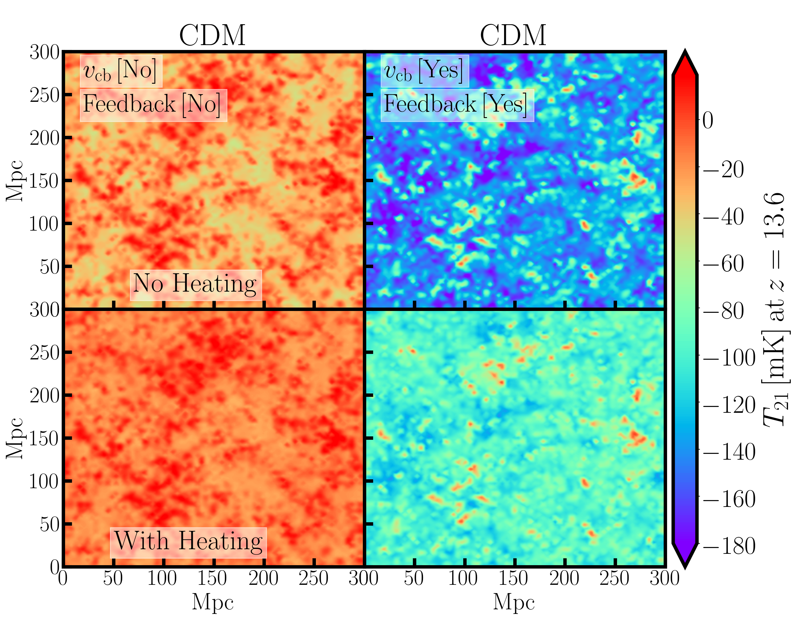
Figure 1: The spatial fluctuations of 21-cm brightness temperature $T_{21}$ (Eq. 1) at $z\!=\!13.6$. Top and bottom panels show results without and with additional heating effects, respectively. The left column corresponds to CDM model without the relative velocity $v_{\rm cb}$ and LW feedback, whereas the right column corresponds to CDM model with both the relative velocity $v_{\rm cb}$ and LW feedback effects. Each result here is obtained from a simulation slice $300$ Mpc in length and $3$ Mpc in thickness. We use $\log_{10}(L_{\rm X}/{\rm SFR})\!=\!39$ for all the simulations.

In Fig. 1, we show the spatial fluctuations of the 21-cm brightness temperature $T_{21}$ (Eq. 1) for CDM at $z=13.6$. The dip of the global signal $\langle T_{21}\rangle$ for the FDM models is very close to this redshift. The top panels show results without the additional heating and the bottom panels show results with additional heating. Considering the top panels, we see that for CDM without $v_{\rm cb}$ and LW feedback, the $T_{21}$ values lie in the range $-50\,{\rm mK}\,\lesssim T_{21}\lesssim 20\,{\rm mK}\,$ and the average temperature $\langle T_{21}\rangle$ $\approx-24$ mK. When we include additional heating, the average temperature of the box rises to $\langle T_{21}\rangle$ $\approx-13$ mK and now the $T_{21}$ values lie in the range $-20\,{\rm mK}\,\lesssim T_{21}\lesssim 20\,{\rm mK}\,$. With $v_{\rm cb}$ and LW feedback, the $T_{21}$ values without (with) additional heating lie in range $-160\,{\rm mK}\,\lesssim T_{21}\lesssim-10\,{\rm mK}\,$ ($-120\,{\rm mK}\,\lesssim T_{21}\lesssim-10\,{\rm mK}\,$) with average value $\langle T_{21}\rangle$ $\approx-135$ mK ($\approx-100$ mK).

In Fig. 2, we compare between the CDM and FDM models at two redshifts, $z=13.6$ and $z=21.1$. At $z=21.1$, both Lyman-$\alpha$ coupling and additional heating are present for CDM, whereas both of these are yet to start for FDM. We find that almost all the pixels of both the FDM boxes show $T_{21}\approx 0$ mK, and there is no visible difference when we either consider or drop the effects of $v_{\rm cb}$ and feedback. On the other hand, the effects of $v_{\rm cb}$, feedback and additional heating are very apparent for the CDM boxes. Without (with) all these effects, the $T_{21}$ values lie in range $-200\,{\rm mK}\,\lesssim T_{21}\lesssim-110\,{\rm mK}\,$ ($-200\,{\rm mK}\,\lesssim T_{21}\lesssim-80\,{\rm mK}\,$) with $\langle T_{21}\rangle$ $\approx-170$ mK ($\langle T_{21}\rangle$ $\approx-100$ mK). Considering FDM results at $z=13.6$, we find that without additional heating, most of the $T_{21}$ value are below $-200$ mK and a few pixels show values around $-100$ mK, with an average $\langle T_{21}\rangle$ $\approx-180$ mK. When the additional heating is included, the average temperature rises to $\langle T_{21}\rangle$ $\approx-150$ mK. Although, the $T_{21}$ values still lie in the range $-200\,{\rm mK}\,\lesssim T_{21}\lesssim-100\,{\rm mK}\,$, more $T_{21}$ values are now close to $-100$ mK which increases the overall average. Note that the highest peak values of $T_{21}$, where we expect the sources to lie, do not change by much when we include additional heating. Only the low $T_{21}$ regions around the highest peaks show increased temperature with additional heating.

From the discussion above, we conclude that both the CDM and FDM models are affected by the additional heating. Overall, additional heating alters the spatial structure of the 21-cm fluctuations. Also, $v_{\rm cb}$ and LW feedback have no visible effects on $T_{21}$ fluctuations for FDM. We will quantify both delaying and heating effects through the 21-cm global signal and power spectrum.

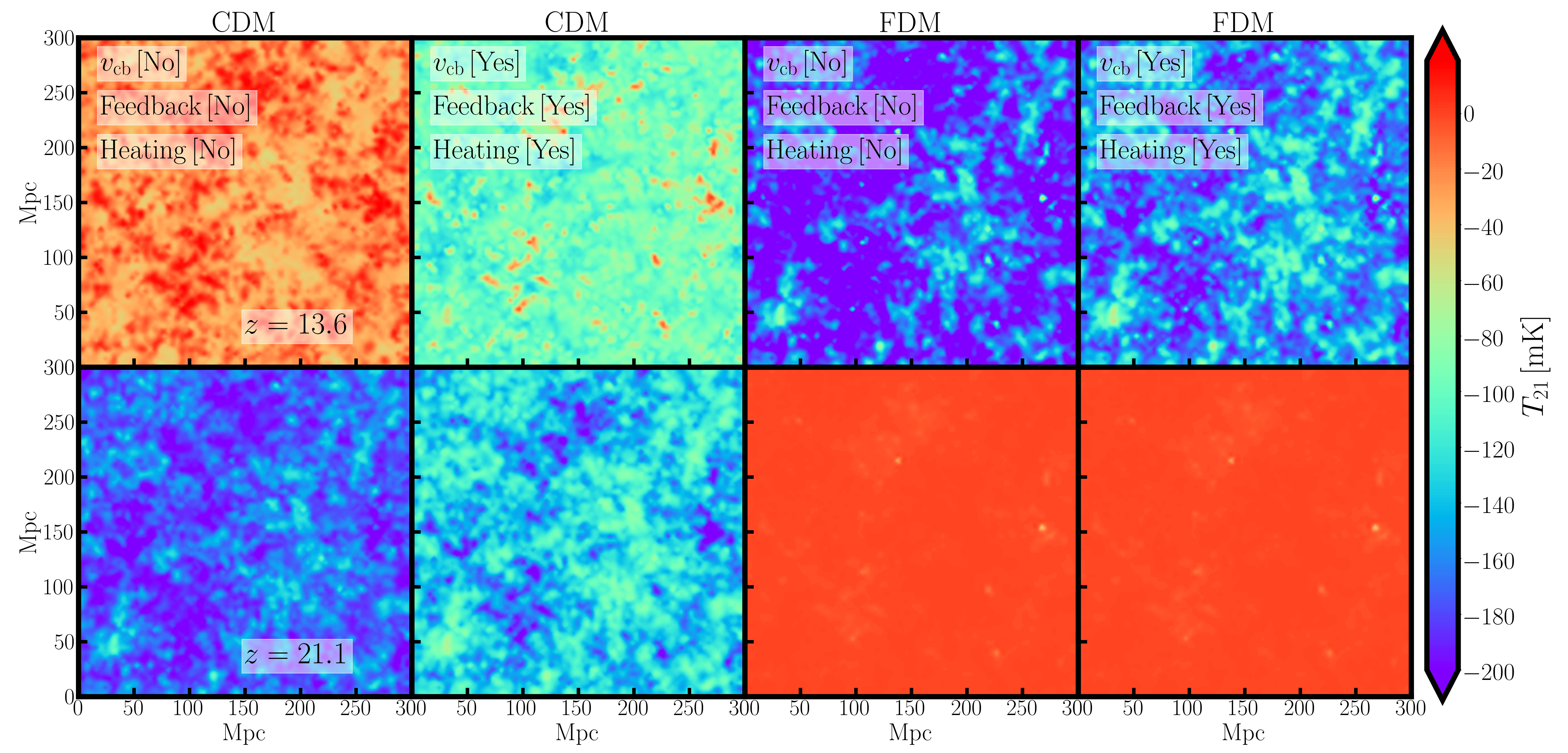
Figure 2: The spatial fluctuations of the 21-cm brightness temperature $T_{21}$ (Eq. (1)) at $z\!=\!13.6$ and $z\!=\!21.1$. The odd and even columns show results without and with additional (Lyman-$\alpha$ and CMB) heating and delaying (relative velocity $v_{\rm cb}$ and LW feedback) effects, respectively. The first two columns show results for CDM and the last two for FDM. Each result here is obtained from a simulation slice $300\,{\rm Mpc}$ in length and $3\,{\rm Mpc}$ in thickness, and setting $\log_{10}(L_{\rm X}/{\rm SFR})\!=\!39$.

IV.2 Global Signal

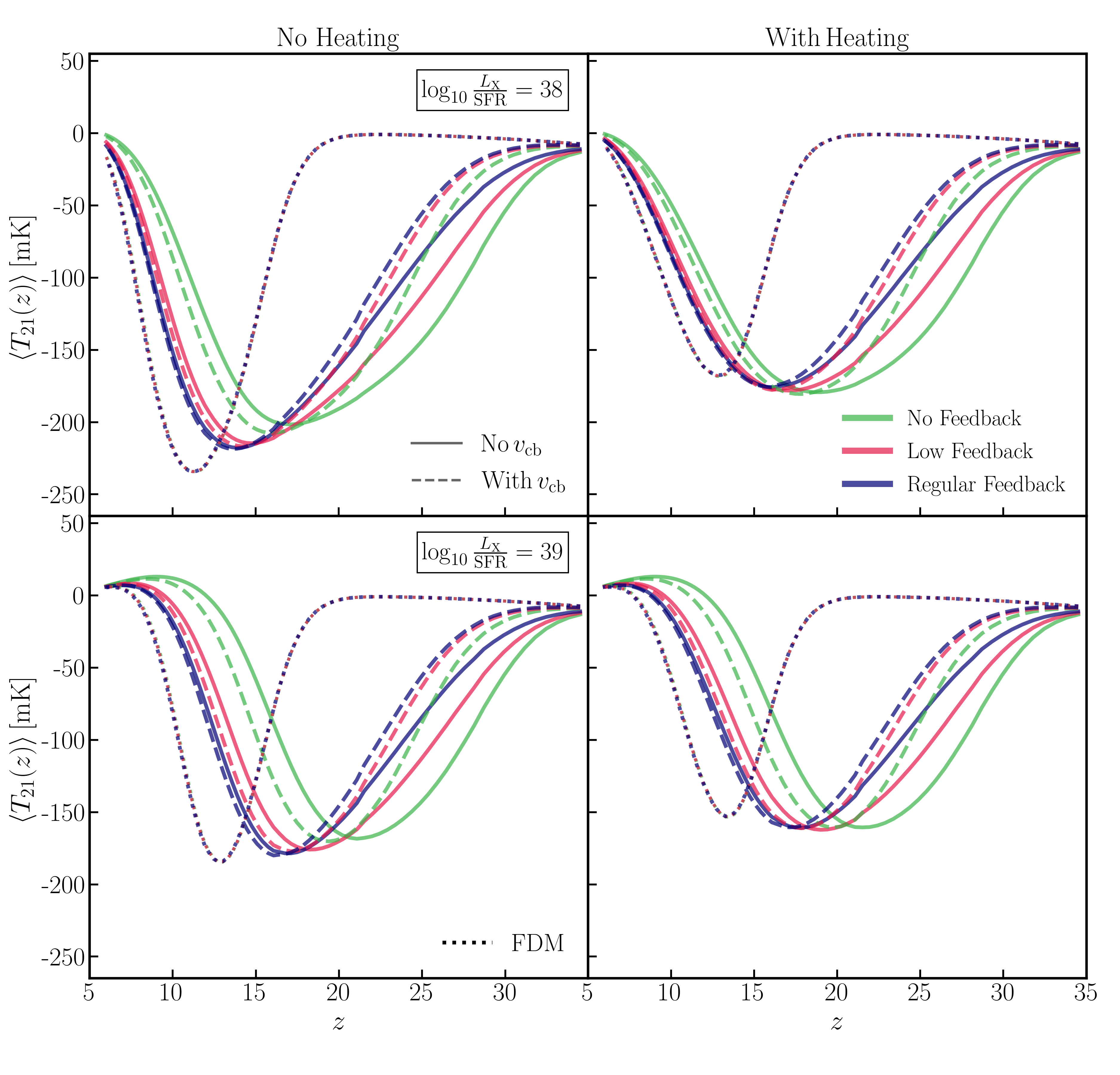
Figure 3: The 21-cm global signals $\langle T_{21}(z)\rangle$ as a function of redshift $z$. The top panels correspond to low X-ray efficiency ($\log_{10}(L_{\rm X}/{\rm SFR})=38$), and bottom panels correspond to moderate X-ray efficiency ($\log_{10}(L_{\rm X}/{\rm SFR})=39$). Solid and dashed curves refer to the CDM models without and with the relative velocity $v_{\rm cb}$ effects, whereas the different colors indicate different LW feedback strengths. As relative velocity $v_{\rm cb}$ does not affect the FDM results, we show those with dotted curves where the different colors indicate different LW feedback strengths. Note that for FDM, the curves with different LW feedback strengths overlap. This again indicates that LW feedback has no effect on FDM.

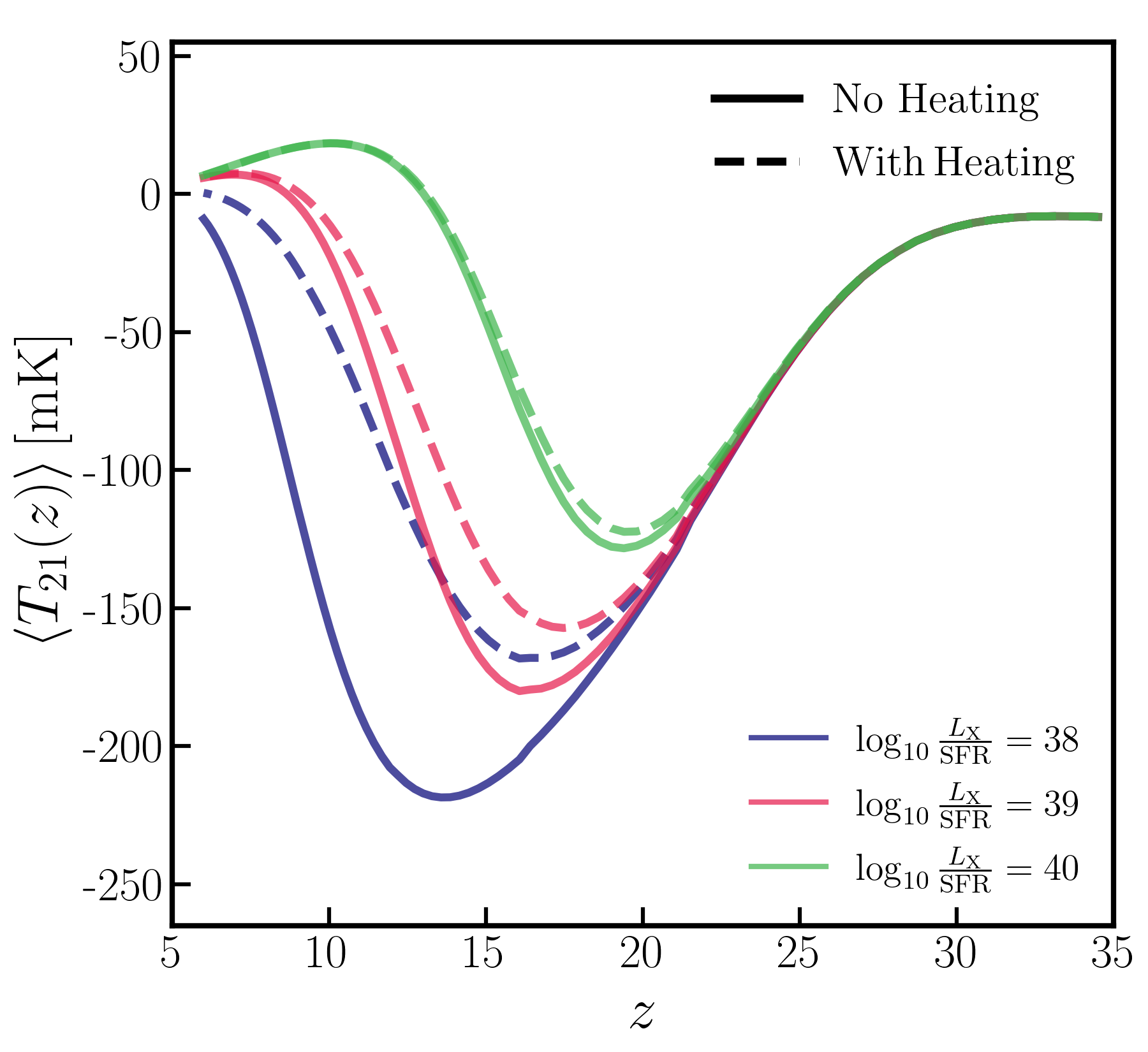
Figure 4: The 21-cm global signals $\langle T_{21}(z)\rangle$ as a function of redshift $z$ for three different X-ray heating efficiencies: low ($\log_{10}(L_{\rm X}/{\rm SFR})=38$), moderate ($\log_{10}(L_{\rm X}/{\rm SFR})=39$) and high ($\log_{10}(L_{\rm X}/{\rm SFR})=40$). All curves are for CDM models without $v_{\rm cb}$ and feedback. The solid and dashed curves correspond to models without and with additional heating effect.

Fig. 3 shows the global signal for both CDM and FDM models with two different X-ray efficiencies, $\log_{10}(L_{\rm X}/{\rm SFR})=38$ and $39$. The overall shape and the minimum value of the signal depend on the various effects like $v_{\rm cb}$, LW feedback and additional heating.

We discuss the different cases one by one. We first consider the top-left panel which shows the global signals for $\log_{10}(L_{\rm X}/{\rm SFR})=38$ (low X-ray efficiency) and without additional heating. For CDM, without LW feedback and $v_{\rm cb}$, we see that the minimum occurs at $z\sim 17$. However, when the LW feedback or $v_{\rm cb}$ is considered, the minimum is shifted towards smaller redshift. Both $v_{\rm cb}$ and LW feedback prevent the formation of luminous structures inside small halos and increase the mass of the smallest halos that can form stars. This process delays the beginning of the Lyman-$\alpha$ coupling era and the minimum of the global signal is shifted to smaller redshift. In presence of both LW feedback and $v_{\rm cb}$, this effect is strongest and the minima for the CDM model occur at the smallest redshift ($z\sim 13$). Moreover, the shape of the signal depends very much on the presence of LW feedback and $v_{\rm cb}$.

In contrast, for the FDM model we see that the shape and the minimum of the global signal do not depend on neither LW feedback nor $v_{\rm cb}$. This is expected, as the length scale below which the halos are suppressed in FDM model is well above the effective Jeans scales of both $v_{\rm cb}$ and LW feedback, i.e. the minimum halo mass that can contain first galaxies in FDM paradigm is well above the minimum halo masses that are affected by the $v_{\rm cb}$ and LW feedback. In the $z$ range of Fig. 3, the kinetic temperature drops off as $(1+z)^{2}$. Therefore, the amplitude of the minimum of the global signal depends on when the Lyman-$\alpha$ coupling saturates and $T_{\rm S}$ couples with $T_{\rm K}$. In the CDM model, $v_{\rm cb}$ and LW feedback delays the star formation, so we get a minimum signal when both $v_{\rm cb}$ and LW feedback are present. Similarly, FDM shows the minimum temperature in comparison to CDM.

However, the above is true when X-ray heating is not very efficient and additional heating sources are not present. In the presence of additional heating (top-right panel), or efficient X-ray heating (bottom-left panel), we see that the minimum of the signal (in comparison to the top-left panel) occurs at slightly higher redshift. This happens because the external heating sources tend to increase $T_{\rm K}$ before the signal reaches the minimum value where the Lyman-$\alpha$ coupling saturates. This effect is maximal when all the heating sources come into play. However, the additional heating is no longer important when we have very efficient X-ray heating. This we can see in the bottom panels, i.e. for $\log_{10}(L_{\rm X}/{\rm SFR})=39$. Here, the curves with (right panel) and without (left panel) additional heating are not very different.

In order to demonstrate this more clearly, we have plotted the CDM results for three different X-ray heating efficiencies in Fig. 4. We see that the solid (without additional heating) and dashed (with additional heating) curves almost overlap for $\log_{10}(L_{\rm X}/{\rm SFR})=40$. This happens when X-ray heating becomes so efficient that it comes into play even before the CMB or Lyman-$\alpha$ heating start to act. Another important difference between the CDM and FDM models is that the additional heating effect is maximal for the FDM models. Note that, between CMB and Lyman-$\alpha$ heating, the former is generally more efficient above a certain redshift and it is sufficient to explain this difference in terms of CMB heating. This is not necessarily correct when multiple scatterings are considered, which we leave to future work. The CMB heating is more efficient if $(T_{\rm rad}/T_{\rm S}-1)$ is larger and $x_{{\rm H\,{\footnotesize I}}}$ is higher. Both of these are true for FDM models in comparison to CDM, which is why the additional heating is more prominent for the FDM models.

Figure 5: The 21-cm power spectrum $\Delta^{2}_{21}(k)$ (Eq. 8) as a function of the wave vector $k$. The top, middle and bottom panels show results for three different X-ray heating efficiencies: low ($\log_{10}(L_{\rm X}/{\rm SFR})=38$), moderate ($\log_{10}(L_{\rm X}/{\rm SFR})=39$) and high ($\log_{10}(L_{\rm X}/{\rm SFR})=40$, respectively. Red and blue colors indicate CDM and FDM models, respectively. Solid, dashed and dotted curves refer to Case-I (no $v_{\rm cb}$, no LW feedback, no additional heating), Case-II (with $v_{\rm cb}$, with regular LW feedback, no additional heating) and Case-III (with $v_{\rm cb}$, with regular LW feedback, with additional heating), respectively. Each column corresponds to a particular redshift which is indicated at the top.

IV.3 Fluctuation Power Spectrum

In this section, we discuss the 21-cm power-spectrum which is defined as

$$\Delta^{2}_{21}(k)=\frac{k^{3}P_{21}(k)}{2\pi^{2}}\,[{\rm mK}^{2}],$$ (8)

where $P_{21}(k)=\langle\tilde{T}_{21}(k)\tilde{T}_{21}^{\ast}(k)\rangle$ and $\tilde{T}_{21}(k)$ is the Fourier transform of $T_{21}-\langle T_{21}\rangle$. Fig. 5 shows the 21-cm power spectra as functions of $k$ for three different X-ray efficiencies, $\log_{10}(L_{\rm X}/{\rm SFR})=38,39,40$. We show our results at four different redshifts: $(i)$ $z=21.1$: which is within CD for the CDM models, $(ii)$ $z=18.2$: where we expect the additional heating effects to start for the CDM models, $(iii)$ $z=13.6$: very close to the dip of the global signal for the FDM models, $(iv)$ $z=7$: towards the end of reionization where $x_{{\rm H\,{\footnotesize I}}}$ drops and we expect X-rays to dominate for very efficient X-ray heating. We see that the power spectra show very different scale dependence at these redshifts for the different models. We have chosen three cases to demonstrate different effects, Case-I: no $v_{\rm cb}$, no LW feedback, no additional heating, Case-II: with $v_{\rm cb}$, with Regular LW feedback but with no additional heating and Case-III: with $v_{\rm cb}$, with Regular LW feedback, and with additional heating.

We first consider the top panels, i.e. power spectra for low X-ray efficiency $\log_{10}(L_{\rm X}/{\rm SFR})=38$. At $z=21.1$, we do not expect the X-ray or even additional heating effects to come into play. Therefore, the shape and amplitude of the power spectra here depend on the onset of the Lyman-$\alpha$ coupling in the different models. The Lyman-$\alpha$ coupling starts early for the CDM models in comparison to FDM models. In absence of Lyman-$\alpha$ coupling, the $T_{\rm S}$ in FDM models is still close to $T_{\rm rad}$. Due to this, we see that the amplitude of the 21-cm power spectra is very low (factor of $>100$ smaller) for the FDM models in comparison to the CDM models. Among the CDM models, relative velocity and LW feedback cut out smaller mass halos and the higher mass halos that remain are highly biased. This enhances the large scale (small $k$) amplitude of the 21-cm power spectrum for Case-II and III in comparison to Case-I. At $z=18.2$, the Lyman-$\alpha$ coupling has already started for the FDM model, $T_{\rm S}$ gets closer to $T_{\rm K}$ and the amplitude of the power spectrum increases for FDM. However, heating is still not started for the FDM models at this redshift. For the CDM models, $v_{\rm cb}$ and LW feedback actually delay the heating, and heating reduces the amplitude of the 21-cm power spectrum as it takes the $T_{\rm K}$ towards $T_{\rm rad}$. This can be seen in this panel as the curve with heating (dotted red) lies below the curve with no heating.

At $13.6$, the FDM models are very close to the dip of the global signal. This implies that the fluctuations are maximally away from $T_{\rm rad}$ and 21-cm fluctuations show maximum power. However, FDM models with heating show a smaller amplitude for the power spectrum. For the CDM models, we see a minimum amplitude for Case-I power spectrum and a maximum amplitude for Case-II power spectrum. Here also, heating reduces the amplitude and Case-III remains below Case-II. At $z=7$, we see similar features as we see in $z=13.6$, only the power in Case-III is smallest here. If we consider the middle and bottom panels, which means if we increase the X-ray heating efficiency, we see that the difference between Case-II and Case-III becomes small for both CDM and FDM. This again shows that the additional heating is not important if the X-ray heating is highly efficient. For $\log_{10}(L_{\rm X}/{\rm SFR})=40$, we see that all the curves almost overlap at $z=7$ which marks the end of the reionization stage. By this time, X-ray heating dominates over the other physical effects and we see almost no difference between CDM and FDM models.

Figure 6: The redshift $z$ evolution of the 21-cm power spectrum $\Delta^{2}_{21}$ at $k=0.1~{}{\rm Mpc}^{-1}~{}$ and $k=0.46~{}{\rm Mpc}^{-1}~{}$. The red and blue colors, respectively, indicate CDM and FDM models, whereas the deep and light shades of those indicate models without and with additional heating. Solid curves show results without the relative velocity $v_{\rm cb}$ and LW feedback, and dashed curves show results with both relative velocity $v_{\rm cb}$ and LW feedback. Here the X-ray heating efficiency is kept fixed at $\log_{10}(L_{\rm X}/{\rm SFR})=39$ for all the curves.

In Fig. 6, we show the redshift dependence of the power spectrum amplitude at two specific $k$ values, for completeness. We first consider the Case-I for CDM at $k=0.1~{}{\rm Mpc}^{-1}~{}$. We can see three distinct epochs where three different effects dominate the fluctuation fields. Fluctuations in Lyman-$\alpha$ coupling dominate at $z>20$ and this contribution peaks around $z\sim 24$ when $x_{\alpha}$ becomes $1$. The dip around $z\sim 20$ marks the transition from the Lyman-$\alpha$ to X-ray heating domination. X-ray heating fluctuations dominate inbetween $10<z<20$ and this peaks around $z\sim 16$. Fluctuations due to X-ray heating reduce and show a dip at $z\sim 10$. Below this redshift, the ionization fluctuations during the reionization epoch dominate and the power spectrum again rises.

At even smaller redshifts ($z<6$, which we do not show here), the power spectrum eventually goes down due to a rapid decline in the neutral fraction $x_{{\rm H\,{\footnotesize I}}}$. These three distinct epochs are clearly visible in all other models, as well as at $k=0.46~{}{\rm Mpc}^{-1}~{}$. Now, when we consider Case-II for CDM, i.e. we include the effects of $v_{\rm cb}$ and LW feedback, we see that all the features (peaks and dips) are shifted toward smaller redshift by roughly $\Delta z\sim 4$. In the range $8<z<25$, the amplitude of the power spectrum is also higher in this case. This again verifies the fact that $v_{\rm cb}$ and LW feedback delay the CD and therefore all the successive epochs.

Comparing the FDM models with CDM, we see a similar effect. The absence of smaller mass halos in FDM delays the onset of the domination of Lyman-$\alpha$ , X-ray and ionization fluctuations, and the corresponding epochs are shifted by $\Delta z\sim 8,5$ and $2$ respectively. Remember that $v_{\rm cb}$ and LW feedback have no visible effects for FDM models. In the range $7<z<19$, the amplitude of the FDM power spectrum is higher than almost all of the CDM models. Now, if we include additional heating, we see that the amplitude of the power spectrum, compared to the no heating cases, decreases below the peak redshift of the Lyman-$\alpha$ epoch for all the models and this remains true until the end of the X-ray heating epoch. This suppression in power is maximal near the peak of the X-ray heating era, and this effect is more prominent for the FDM models. The additional heating decreases the amplitude of the power spectrum as it increases $T_{\rm K}\approx T_{\rm S}$ and overall decreases the contrast $(T_{\rm rad}-T_{\rm S})$. The additional heating also shifts the peaks and the dips, but only very slightly. Considering the right panel, we observe that the above discussion is qualitatively true for $k=0.46~{}{\rm Mpc}^{-1}~{}$ as well.

V Forecast with HERA

V.1 Sensitivity Calculation

In this section, we discuss the possibility of measuring the 21-cm power spectrum using the upcoming HERA 21-cm intensity mapping experiment [25]. HERA is located in the Karoo Desert of South Africa and is designed to measure the 21-cm fluctuations from CD ($50$ MHz or $z\sim 27$) to the reionization era ($225$ MHz or $z\sim 5$). The final stage of HERA is expected to have $350$ antenna dishes, each with a diameter of $14$ m. Out of the $350$ dishes, $320$ will be placed in a close-packed hexagonal configuration and the remaining $30$ will be placed at longer baselines. HERA will mainly operate as a drift scan telescope where the telescope will point toward the zenith and the scanning will be done as the Earth rotates.

We calculate the sensitivity of HERA using the publicly available package 21cmSense  [73, 74]. This code accounts for the $u-v$ sensitivities of each antenna in the array, and calculates the possible errors in the 21-cm power spectrum measurement, including cosmic variance. The 21cmSense package assumes a receiver temperature of $100$ K and a sky temperature of $T=60\,{\rm K}\,(\nu/300\,{\rm MHz})^{-2.55}$, and the combination of both is called the system temperature $T_{\rm sys}$. We assume a total observing time of $1080$ hours to calculate the sensitivity of HERA. The measurements of the power spectrum are assumed to be done in bandwidths of $8\,{\rm MHz}$ and simultaneously across the redshift range $z=6$ to $27$. Although these simultaneous measurements across a large $z$ range are practically impossible [79], this assumption will provide us some useful insight which is sufficient for this analysis.

The real challenge in 21-cm observations are the Galactic and extra-galactic foregrounds which plague the tiny 21-cm signal [75, 76, 77, 78]. However, the foregrounds are expected to be spectrally smooth, while the 21-cm signal has some spectral structure. This property assures that the foregrounds can be removed to recover the 21-cm signal. The spectral smoothness of the foregrounds also suggests that they should only contaminate the low-order $k_{\parallel}$ (line-of-sight component of the $k$ vector) modes. However, the chromatic response of the telescope, which causes the mode mixing, helps the foregrounds to contaminate the larger $k_{\parallel}$ modes. Still, the foreground contamination is expected to be contained within a region (known as the “foreground wedge”) [74], the boundary of which can be mathematically expressed as

$$k_{\parallel}=W(z)k_{\perp}\,,$$ (9)

where $W(z)$ is a $z$-dependent factor and $k_{\perp}$ is the component of the $k$ vector perpendicular to the line-of-sight. Eq. (9) also marks the “horizon limit” when the $k_{\parallel}$ mode on a given baseline corresponds to the chromatic sine wave created by a flat-spectrum source of emission located at the horizon [80]. A foreground contamination due to spatially unclustered radio sources at the horizon, with a frequency-independent emission spectrum, will lie below this line and we should observe the clean 21-cm signal above this line. However, due to some spectral features in the foregrounds, calibration error etc., foregrounds may contaminate the $k$ space beyond the horizon limit [80]. Based on the above possibilities, the 21cmSense package considers three foreground contamination scenarios: “pessimistic”, “moderate” and “optimistic”. In the moderate scenario, the wedge is assumed to extend to $\Delta k_{\parallel}=0.1h~{}{\rm Mpc}^{-1}~{}$ beyond the horizon wedge limit. In the optimistic scenario, the boundary of the foreground wedge is set by the FWHM of the primary beam of HERA and there is no contamination beyond this boundary. Finally, in the pessimistic scenario, the foreground wedge extends $\Delta k_{\parallel}=0.1h~{}{\rm Mpc}^{-1}~{}$ beyond the horizon limit, and only the instantaneously redundant baselines are combined coherently.

V.2 Distinguishing between CDM and FDM

The possibility of discrimination between CDM and FDM models depends on the error with which we shall be able to measure the 21-cm power spectrum. In order to gauge this possibility, we calculate the chi-square difference $\Delta\chi^{2}$ which is essentially the mod of the difference of the power spectra between CDM and FDM divided by the expected measurement error. In calculating this $\Delta\chi^{2}$, we assume that CDM is the correct model. We have plotted the $\Delta\chi^{2}$ calculated using the 21-cm power spectrum in the top panels of Fig. 7. For comparison, we have also plotted the $\Delta\chi^{2}$ for the global signal in the bottom panels of Fig. 7. For global signal, we have assumed an error of $5$ mK throughout the $z$ range.

Figure 7: We show $\Delta\chi^{2}$, the statistical significance with which HERA can distinguish between CDM and FDM models, at different redshifts. Top and bottom panels show results for power spectrum and global signal, whereas the different columns show results for different X-ray heating efficiencies, indicated at the top. Different colors on the top panels refer to different foreground contamination scenarios. Solid, dashed and dotted curves correspond to Case-I (no $v_{\rm cb}$, no LW feedback, no additional heating), Case-II (with $v_{\rm cb}$, with regular LW feedback, but no additional heating) and Case-III (with $v_{\rm cb}$, with regular LW feedback, and with additional heating), respectively. The particle mass in the FDM model is $m_{\rm FDM}=10^{-21}\,{\rm eV}$. The shaded region show below $5-\sigma$ detection limit.

Comparing the top and bottom panels, it is evident that the power spectrum has more discriminating power than the global signal. The maximum $\Delta\chi^{2}$ is $\sim 30$ for the global signal, whereas it is $\sim 2000$ for the power spectrum. For the global signal with the lowest X-ray heating, we find that the Case-I shows the maximum $\Delta\chi^{2}$ at most of the redshifts in comparison to other cases. This is also true for other X-ray heating cases. However, when we introduce relative velocity $v_{\rm cb}$, LW feedback (Case-II) and additional heating (Case-III), we find that the overall $\Delta\chi^{2}$ drops, although Case-II and III show higher $\Delta\chi^{2}$ than Case-I in a small $z$ range around $z\sim 17$ (note that this depends on X-ray heating) . Below $z\sim 18$, we see some difference in $\Delta\chi^{2}$ between Case-II and III for the lowest X-ray heating. This difference fades away as the X-ray efficiency increases.

Considering the results for the power spectrum (top panels), we see that at $z<17$, $\Delta\chi^{2}$ values are higher for Case-I in all foreground contamination scenarios. This changes for the optimistic foregrounds and we see that at $z>17$ Case-II and Case-III show higher $\Delta\chi^{2}$ in comparison to Case-I. For the moderate and pessimistic foregrounds, this is true, but for a very limited redshift range. From Figs. 5 and 6, we see that for CDM in this range, the power spectrum amplitude is higher at small $k$ in Case-II and III in comparison to Case-I. The combination of this and the small error for the optimistic foregrounds make $\Delta\chi^{2}$ higher for Case-II and III. Considering the optimistic foregrounds for Case-I with lowest X-ray heating, we see that the highest peak of $\Delta\chi^{2}$ ($\sim 2000$) occurs at $z\sim 7$ and the second highest peak ($\sim 300$) occurs at $z\sim 13$. Note that we have several peaks in these $\Delta\chi^{2}-z$ plots, and their locations depend on the delay in different processes between CDM and FDM models, and also on the choice of astrophysical parameters. We shall mainly focus on the first two highest peaks. When we introduce $v_{\rm cb}$ and LW feedback effects (Case-II), we see that the peak values are suppressed ($\sim 300$ for the first peak and $\sim 150$ for the second). Additional heating drops the peak values further ($\sim 70$ for the first peak and $\sim 150$ for the second) and it has maximum effect on the first peak. The above is true for moderate and pessimistic backgrounds, only the peak values change. For the moderate and high X-ray heating, we see that the peak locations and their amplitudes change. Peak amplitude is lowest for the highest X-ray heating. All the discussion for the lowest X-ray heating also holds for moderate and high X-ray heating. However, the effect due to the additional heating decreases with increase in X-ray efficiency and is minimal for $\log_{10}(L_{\rm X}/{\rm SFR})=40$.

Overall, the discussion above suggests that the presence of $v_{\rm cb}$ and LW feedback (which mainly affect CDM), along with any heating, be it X-ray or additional (which affect both CDM and FDM), lowers our ability to discriminate between the CDM and FDM models.

Figure 8: This shows $\Delta\chi^{2}_{\rm tot}$, which is the sum of $\Delta\chi^{2}$ (Fig. 7) over all the $z$ values, for the different values of $m_{\rm FDM}$. For all the results we fix $\log_{10}(L_{\rm X}/{\rm SFR})=39$. Different colours show different foreground contamination scenarios. Star, circle and square markers correspond to Case-I (no $v_{\rm cb}$, no LW feedback, no additional heating), Case-II (with $v_{\rm cb}$, with regular LW feedback, but no additional heating) and Case-III (with $v_{\rm cb}$, with regular LW feedback, and with additional heating), respectively. We place two horizontal lines to show the $1-\sigma$ and $5-\sigma$ detection limits.

Finally, we explore the possibility of distinguishing the CDM and FDM models for different $m_{\rm FDM}$. Note that, as $m_{\rm FDM}$ increases, FDM results approach CDM results. There will be a maximum limit in $m_{\rm FDM}$, above which the CDM and FDM models cannot be differentiated with HERA. We investigate this limit in Figure 8 which shows $\Delta\chi^{2}_{\rm tot}$, the sum of $\Delta\chi^{2}$ (Figure 7) over all the $z$ values, for four different $m_{\rm FDM}$ values between $10^{-21}\,{\rm eV}$ and $10^{-18}\,{\rm eV}$. $\Delta\chi^{2}_{\rm tot}$ broadly determines the overall discriminating power of HERA. We choose two values of $\Delta\chi^{2}_{\rm tot}$, $1$ ($68\%$ confidence) and $5$ ($99.99\%$ confidence), as metric of discriminating power. Considering the optimistic foreground scenario, we find that HERA is able to discriminate between CDM and FDM models (for all the three cases considered) up to $m_{\rm FDM}\approx 10^{-18}\,{\rm eV}$ with $68\%$ confidence and up to $m_{\rm FDM}\approx 10^{-19}\,{\rm eV}$ with $99.99\%$ confidence. When we consider moderate and pessimistic foreground contamination, the same limits go down by an order, and HERA is able to tell apart the CDM and FDM models up to $m_{\rm FDM}\approx 10^{-19}\,{\rm eV}$ with $68\%$ confidence and up to $m_{\rm FDM}\approx 10^{-20}\,{\rm eV}$ with $99.99\%$ confidence. Note that if we consider only Case-I—incorporating neither $v_{\rm cb}$, feedback nor additional heating—then HERA is able to differentiate between CDM and FDM up to $m_{\rm FDM}\approx 10^{-19}\,{\rm eV}$ with $99.99\%$ confidence even for the moderate and pessimistic foreground contamination scenario. This would overestimate the 21-cm $m_{\rm FDM}$ bound by an order of magnitude.

V.2.1 Comparison with 21cmFast 3.1.3

While the writing of this paper was in progress, Ref. [60] came out with the release of 21cmFast version 3.1.3. This python-based version includes the delaying effects of $v_{\mathrm{cb}}$ and the LW feedback, as well as the separation of Pop-II and Pop-III stars into molecular and atomic cooling halos, respectively.

In a similar manner to our implementation in 21cmvFast, we have incorporated the Lyman-$\alpha$ and CMB heating effects as well as the FDM transfer function in 3.1.3. We compare the global signals of the two versions in Fig. 9, for Case-II and Case-III. Most noticeably, we see that the CDM signals are significantly delayed in the new version of 3.1.3. This is mainly due to the new modelling of the star formation rate density in 3.1.3.

We have also repeated the $\Delta\chi^{2}$ analysis in 3.1.3. Since the CDM signal (global and power spectrum) is delayed in 3.1.3 (compared to 21cmvFast), the difference between the CDM and FDM scenarios becomes less pronounced. However, this is compensated by the fact that the HERA sensitivity is considerably higher at lower redshifts. Overall, we find that under the modelling of 3.1.3, the FDM scenario is more easily detectable, but none of our conclusions change by more than roughly a factor two. In particular, we find using version 3.1.3 as well that the heating effects reduce the ability of HERA to distinguish between CDM and FDM, as expected.

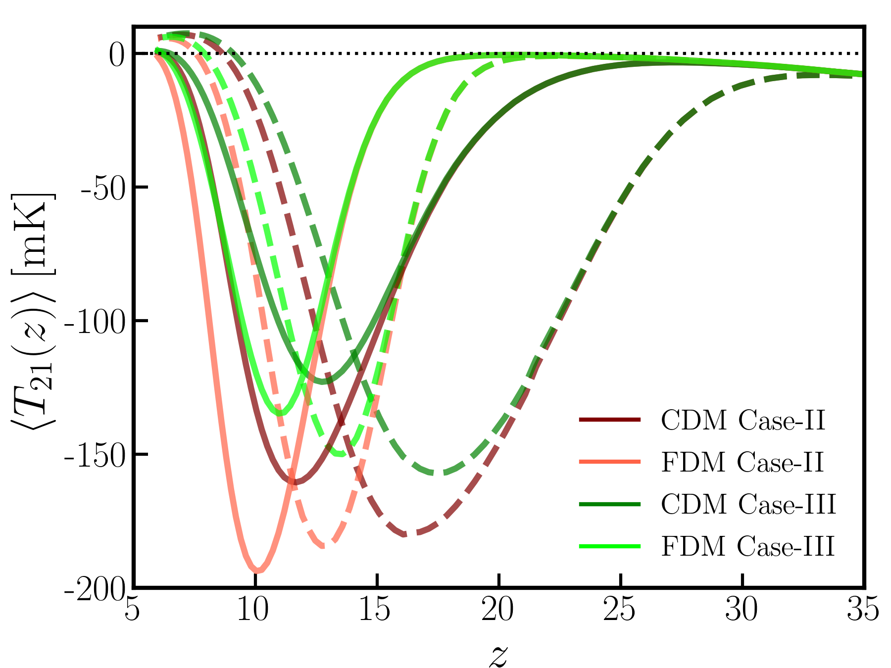
Figure 9: Comparison of the 21-cm global signals between 21cmvFast (dashed) and 21cmFast 3.1.3 (solid). For 21cmvFast we use the fiducial values of Table 1, while for 21cmFast 3.1.3 we adopt the EOS2021 values (see Table 1 in Ref. [60]), and in both versions we set $\log_{10}(L_{X}/\mathrm{SFR})=39$. For the FDM cases, we set $m_{\mathrm{FDM}}=10^{-21}\,\mathrm{eV}$. The different cases shown here correspond to the same cases as in Fig. 7 and Fig. 8.

V.3 Fisher Matrix Forecasts

Analyses in the previous section convince us that HERA has a high possibility to distinguish between the CDM and FDM models. Now, if we consider FDM to be the true model, then it becomes important to estimate how well we can constrain the different parameters of the model. We use the Fisher matrix formalism to calculate the possible accuracy with which we can estimate the FDM model parameters for the HERA observations. The Fisher matrix may be written as [81, 82, 83]

$$F_{\alpha,\beta}=\sum_{k,z}\frac{\partial\Delta^{2}_{21}(k,z)}{\partial\alpha}\frac{\partial\Delta^{2}_{21}(k,z)}{\partial\beta}\frac{1}{{\rm var}\left[\Delta^{2}_{21}(k,z)\right]}\,,$$ (10)

where $(\alpha,\beta)$ represent different parameters of the model and the sum runs over all the $k$ modes and redshifts. Here, ${\rm var}\left[\Delta^{2}_{21}(k,z)\right]$ is the expected variance for the observable $\Delta^{2}_{21}(k,z)$ which we calculate using the 21cmSense package (Section V.1). Here we have assumed that the different $k$ and $z$ bins are independent.

The inverse of this Fisher matrix $[F_{\alpha,\beta}]^{-1}$ gives us the covariance matrix $C_{\alpha,\beta}$ for the errors in different parameters. We have considered three astrophysical parameters: $\log_{10}(L_{\rm X}/{\rm SFR})$ ($39$ and $40$), $\zeta$ ($20$), $f^{0}_{\ast}$ ($0.05$), and four cosmological parameters: $h$ ($0.6766$), $\Omega_{m0}$ ($0.3111$), $\Omega_{b0}$ ($0.0489$), $m_{\rm FDM}$ ($10^{-21}\,{\rm eV}$), with fiducial values given inside the brackets, for our analysis. For the FDM particle mass $m_{\rm FDM}$, we consider $\log_{10}m_{\rm FDM}$ as a parameter for numerical reasons. Note that we have several other astrophysical and cosmological parameters (see table 1) in our model. One should really take all the parameters into consideration for any real analysis. Then the unimportant parameters can be marginalized if required. However, including more parameters generally degrades the constraints. Also, not all the parameters are equally important. For example, the parameters $B$ (determines the LW feedback strength, and appears in eq. (11) of ref. [61]), $V^{(0)}_{\rm cool}$ and $V^{{\rm H\,{\footnotesize I}}}_{\rm cool}$ are not very important for the FDM analysis. FDM models suppress halos much more massive than molecular cooling threshold $M_{\rm cool}$ (eq. (11) of ref. [61]), which depends on both $v_{\rm cb}$ and $B$. Hence, FDM models are not sensitive to both $V^{(0)}_{\rm cool}$ and $B$. Similarly, $V^{{\rm H\,{\footnotesize I}}}_{\rm cool}$ or $M^{{\rm H\,{\footnotesize I}}}_{\rm cool}$ (which appear in eq. (12) of ref. [61]) have a weak effect on the power spectrum, as well as on the global signal. Other astrophysical parameters like $\lambda_{\rm MFP}$, $\alpha_{X}$, $E_{\rm min}$, and cosmological parameters such as $\sigma_{8,0}$ or $n_{s}$ have some effect on the signal. However, to limit our discussion, we choose not to include them in our analysis.

Models	Foreground	$\log_{10}\frac{L_{\rm X}}{{\rm SFR}}$	$\zeta$	$f^{0}_{\star}$	$h$	$\Omega_{m0}$	$\Omega_{b0}$	$\log_{10}m_{\rm FDM}$ $\left(\frac{\Delta m_{\rm FDM}}{m_{\rm FDM}}\%\right)$
$\Delta^{2}_{21}$, Case-II, Moderate X-ray	Optimistic	0.0015	0.12	0.00042	0.0014	0.00088	0.00016	0.0042 ($1.0\%$)
	Moderate	0.0074	0.51	0.0016	0.0054	0.0011	0.00062	0.017 ($3.8\%$)
	Pessimistic	0.01	0.69	0.0022	0.0072	0.0017	0.00084	0.024 ($5.4\%$)
$\Delta^{2}_{21}$, Case-III, Moderate X-ray	Optimistic	0.0046	0.12	0.00078	0.002	0.00079	0.00022	0.006 ($1.4\%$)
	Moderate	0.021	0.52	0.0035	0.0094	0.0036	0.0011	0.027 ($6.03\%$)
	Pessimistic	0.029	0.73	0.0049	0.013	0.0051	0.0016	0.038 ($8.4\%$)
$\Delta^{2}_{21}$, Case-III, High X-ray	Optimistic	0.0053	0.077	0.0015	0.0013	0.00062	0.00019	0.0084 ($1.9\%$)
	Moderate	0.03	0.53	0.012	0.004	0.0019	0.0011	0.067 ($14.3\%$)
	Pessimistic	0.043	0.76	0.018	0.0054	0.0025	0.0015	0.098 ($20.2\%$)
Global, Case-III, Moderate X-ray		0.38	9.15	0.042	0.062	0.059	0.008	0.22 ($39.7\%$)

Table 2: $1-\sigma$ constraints on the parameters with HERA observations for different models. The different foreground contamination scenarios are indicated in the different rows. For high X-ray efficiency, there is not much difference between Case-II and III, so we show results only for Case-III. We also show results for global signal (bottom row) with an error of $5$ mK throughout the redshift range.

As the FDM particle mass is an important quantity in our study, we briefly discuss the correlation of FDM particle mass with other parameters. Overall, we see that it is very much degenerate with other parameters. An increase in the FDM particle mass lowers the suppression effect and increases the number of smaller halos. This reduces the delay in structure formation, which in turn makes CD, the X-ray heating era and the EoR occur earlier. The same can be achieved by increasing $f^{0}_{\star}$, $\log_{10}\frac{L_{\rm X}}{{\rm SFR}}$ and $\zeta$. Therefore, all these parameters are expected to be negatively correlated with $\log_{10}m_{\rm FDM}$ as the effects of increasing $\log_{10}m_{\rm FDM}$ can be compensated by decreasing any of these three parameters. However, in Fig. 10, we find that $\log_{10}m_{\rm FDM}$ is positively correlated with $\log_{10}\frac{L_{\rm X}}{{\rm SFR}}$ and $\zeta$. As discussed in Ref. [36], this is not surprising. $f^{0}_{\star}$, $\log_{10}\frac{L_{\rm X}}{{\rm SFR}}$ and $\zeta$ are not independent, but rather degenerate with each other, and also with the cosmological parameters. As a result, effects due to a change in one parameter can be compensated by a combination of different changes in other parameters. For a particular choice of fiducial values, the correlation between any two parameters can be changed. However, the degeneracy between these parameters can be broken in the following way. $f^{0}_{\star}$ is important during the Lyman-$\alpha$ coupling era, $\log_{10}\frac{L_{\rm X}}{{\rm SFR}}$ mainly affects the X-ray heating era and $\zeta$ is particularly important during Reionization. Therefore, observing these different eras separately can help break the degeneracy. Considering cosmological parameters, we see that $\log_{10}\frac{L_{\rm X}}{{\rm SFR}}$ is positively correlated with $\Omega_{b0}$ and $\Omega_{m0}$, and negatively correlated with $h$.

Our results below suggest that HERA should be able to determine the FDM particle mass to within a few percent in the moderate foreground scenario, at $1-\sigma$ confidence. This suggests that it is possible to have a tight constraint on the FDM particle mass from HERA observations assuming the fiducial value of $m_{\rm FDM}=10^{-21}\,{\rm eV}$. Instead of FDM, had we assumed CDM to be the correct model, the tight constraints would indicate that the upper limit in FDM mass would be tighter than $10^{-21}\,{\rm eV}$ in the CDM model. The constraints on different parameters for various scenarios are given in Table 2.

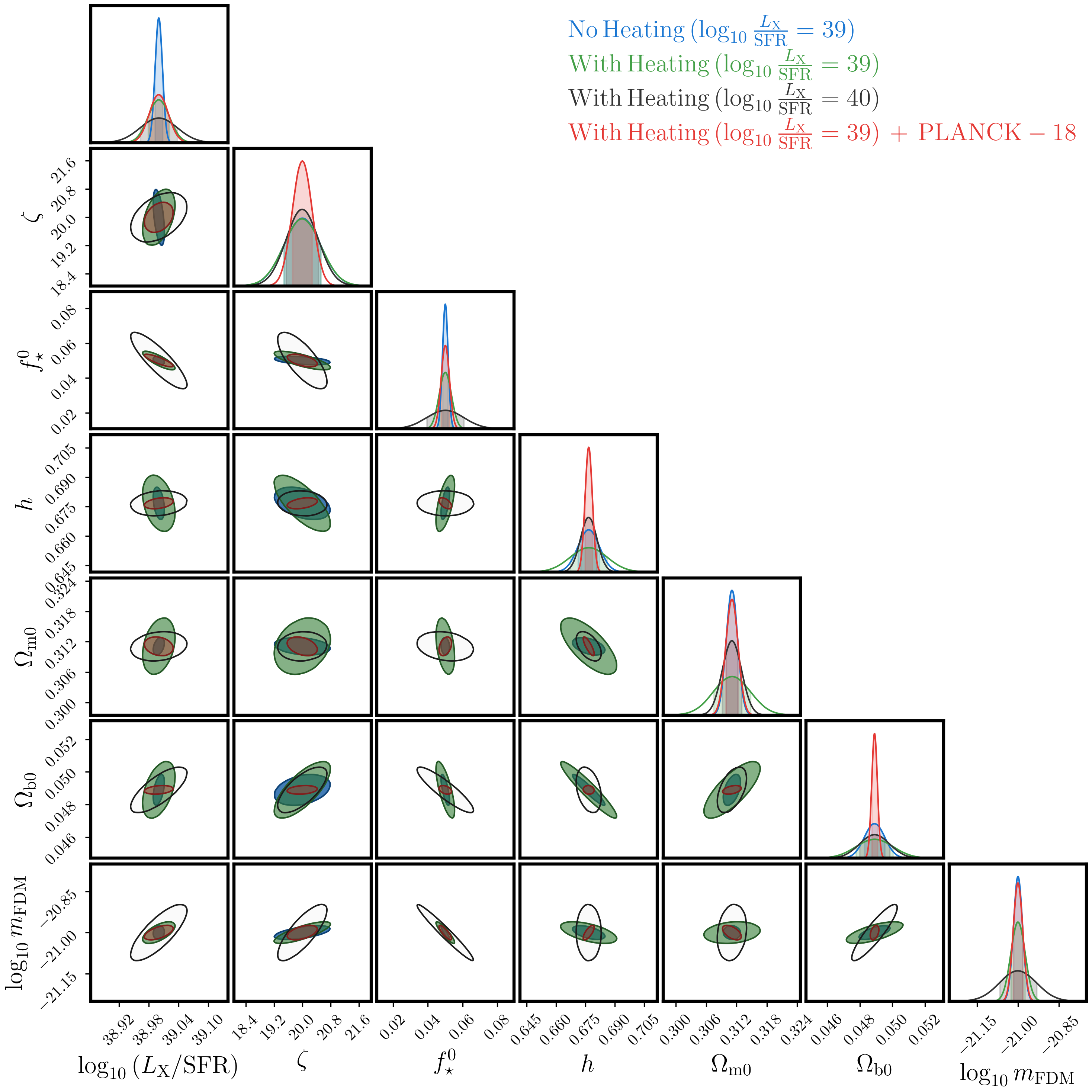
Figure 10: Effects on the parameter constraint forecasts for HERA in presence of additional heating. Blue and Green ellipses correspond to models without and with additional heating for a fixed value of X-ray efficiency $\log_{10}\frac{L_{\rm X}}{{\rm SFR}}=39$. For comparison, we have also plotted results for $\log_{10}\frac{L_{\rm X}}{{\rm SFR}}=40$ with additional heating. In addition, we add to our Fisher matrix the covariance matrix calculated for PLANCK-18 [84] CMB data using a separate MCMC analysis (see Ref. [93] for details) and show the results in red. The PLANCK data is added only for $\log_{10}\frac{L_{\rm X}}{{\rm SFR}}=39$ with additional heating. The ellipses span $1-\sigma$ confidence intervals. All the results correspond to the moderate foreground contamination scenario. Note that the black ellipse of $L_{X}=40$ is centered at 39, to facilitate a comparison.

In Fig. 10, we show the comparison of covariance between the Case-II, which has no additional heating, and Case-III, which includes additional heating. We have shown results for moderate X-ray efficiency and with moderate foreground scenario. We immediately see that the ellipses with no additional heating are smaller than the ones with additional heating. This implies that the additional heating actually degrades the parameter constraints. The presence of additional heating decreases the amplitude of the power spectrum below $z\sim 17$ and this in turn reduces the SNR. However, at $z>18$, the additional heating is not present and we expect to have similar results for both the cases.

A careful inspection shows that the parameter $\zeta$ is not affected much by the additional heating. $\zeta$ is important during the reionization when the heating effects are generally subdominant. We also see that the correlation in most of the parameters are some what different in the two cases. Considering the constraints on $m_{\rm FDM}$ (Table 2), we see that, without additional heating (Case-II) HERA should be able to determine the FDM particle mass to within $1\%$, $3.8\%$ and $5.4\%$ in the optimistic, moderate, and pessimistic foreground scenarios, respectively, at $1-\sigma$ confidence. This is a factor of $\sim 1.5$ better than in Case-III.

For comparison, we have also shown results for Case-III with high X-ray efficiency. We see that the constraints on the most of the parameters degrade for high X-ray efficiency, except for $h$ and $\Omega_{m0}$. Constraints on $h$ and $\Omega_{m0}$ are better for high X-ray efficiency. Also, $h$ and $\Omega_{m0}$ show mild correlation with $\log_{10}m_{\rm FDM}$. In the case of high X-ray, HERA should be able to determine the FDM particle mass to within $14.3\%$ in the moderate foreground scenario at $1-\sigma$ confidence. The same is $1.9\%$ and $20.2\%$ in optimistic and pessimistic foreground scenarios, which we do not show here (see Table 2). Note that, for high X-ray, the additional heating effect is almost negligible and there is not much difference in results between Case-II and Case-III. Hence we do not show the results of Case-II for high X-ray efficiency.

We have also studied the implications of adding the PLANCK-18 [84] covariance matrix on the astrophysical parameters. We use a dedicated MCMC analysis to derive the covariance matrix from PLANCK-18 CMB data, and add it to our 21-cm Fisher matrix. In the future, thanks to the direct interface to CLASS, our code will enable joint MCMC 21-cm-CMB real-data analyses to test the standard cosmological model or any extensions to it.

As expected, PLANCK measures the cosmological parameters with great precision. Here, the idea is to check the improvement in the constrains on the astrophysical parameters when the uncertainty in the cosmological parameters is minimized. Generally tight priors on a set of parameters help in reducing the error in other parameters. Indeed we see exactly this. We add the PLANCK information only to the Case-III with moderate X-ray. We see that the priors result in a significant improvement and the results are comparable to that with Case-II. The constraint on $\log_{10}m_{\rm FDM}$ is very close to that obtained for Case-II.

Lastly, mostly as a fact-check, we have plotted the covariance ellipses for the global signal at moderate X-ray, in comparison to the same ellipses for the power spectrum (not shown in this paper). We find that the ellipses for the power spectrum look minuscule in comparison to the global signal ellipses — we do not have very good constraint on any variable for the global signal, which is expected. The global signal lacks the information on the different length scales which the power spectrum possesses. This gives the power spectrum more constraining power. Nevertheless, a global signal experiment with an overall redshift-independent sensitivity of $5$ mK should be able to determine the FDM particle mass to within $39.7\%$ at $1-\sigma$ confidence. This error, of course, can be minimized by applying priors on the different parameters.

VI Summary and Conclusions

We have simulated the effects of FDM on the 21-cm global signal and power spectrum. Extending previous works, we incorporated in our simulations several important effects on the 21-cm signal, such as the DM-baryon relative velocity $v_{\rm cb}$, LW radiative feedback, and CMB and Lyman-$\alpha$ heating, and studied their impact on the 21-cm signal. For completeness, we also included the results for CDM with all the effects and compared those with the FDM results.

The suppression in the number of small halos in the FDM model delays the onset of CD, the ensuing epoch of heating and also the EoR, in comparison to CDM. The signature of this delay can be seen clearly in the global 21-cm signal, as well as in the 21-cm power spectrum. FDM also influences the spatial structure of the 21-cm fluctuations. The absence of the small halos in the FDM model makes the ionizing sources more biased in comparison to CDM model. The DM-baryon relative velocity $v_{\rm cb}$ and LW radiative feedback also delay the different epochs. However, these only affect CDM models, as the length scale below which the halos are suppressed in FDM is well above the effective Jeans scales of both $v_{\rm cb}$ and LW feedback.

The additional heating, which is a combination of CMB and Lyman-$\alpha$ heating in our analysis, affects both FDM and CDM models. Additional heating increases the minimum value of the absorption signal and shifts the redshift of the minimum. Additional heating also alters the amplitude of the power spectrum. Also, the effect of additional heating is maximal for the FDM models, compared to CDM. This effect, however, is important only when the X-ray heating is not very efficient.

We have investigated the prospects to distinguish between the CDM and FDM models (for fixed FDM particle mass $m_{\rm FDM}=10^{-21}\,{\rm eV}$) by means of $\Delta\chi^{2}$ values, considering both the global signal and fluctuations. For global signal experiments, we have considered a $5$ mK uncertainty throughout the $z$ range. For the fluctuations, we have considered the future HERA observations with three foreground contamination scenarios: optimistic, moderate and pessimistic. We find that the power spectrum is far superior (higher $\Delta\chi^{2}$ values) to the global signal in differentiating the CDM and FDM models. However, $\Delta\chi^{2}$ values drop as we introduce $v_{\rm cb}$, LW feedback or additional heating. The $\Delta\chi^{2}$ values also vary with X-ray heating efficiency, and we see the lowest $\Delta\chi^{2}$ for the highest X-ray efficiency. Therefore, all the additional effects, like $v_{\rm cb}$, LW feedback, heating, lower our ability to discriminate between CDM and FDM models.

Considering different $m_{\rm FDM}$ values in the range $10^{-21}\,{\rm eV}$ to $10^{-18}\,{\rm eV}$, we find that HERA is able to distinguish between the CDM and FDM models up to $m_{\rm FDM}\approx 10^{-18}\,{\rm eV}$ ($10^{-19}\,{\rm eV}$) with $1-\sigma$ ($5-\sigma$) confidence in optimistic foreground scenario, and $m_{\rm FDM}\approx 10^{-19}\,{\rm eV}$ ($10^{-20}\,{\rm eV}$) with $1-\sigma$ ($5-\sigma$) in both moderate and pessimistic foreground scenario.

We have also shown Fisher matrix forecasts for the 21-cm power spectrum. We have considered three astrophysical parameters and four cosmological parameters, including the FDM particle mass $m_{\rm FDM}=10^{-21}\,{\rm eV}$. We find that $m_{\rm FDM}$ is correlated with astrophysical parameters, as well as cosmological parameters. In addition, the astrophysical parameters are themselves correlated with each other. This correlation, however, can be broken by observing the signal form different epochs. For moderate X-ray heating efficiency ($\log_{10}\frac{L_{\rm X}}{{\rm SFR}}=39$) and in the presence of additional heating, we find that HERA should be able to determine the FDM particle mass to within $1.4\%$, $6.03\%$ and $8.4\%$ in the optimistic, moderate, and pessimistic foreground scenarios, respectively, at $1-\sigma$ confidence. These constraints improve by a factor of $\sim 1.5$, if we do not consider the additional heating. The constraints degrade when we consider high X-ray heating efficiency. In addition, we find that the global signal provides a much poorer, $\mathcal{O}(1)$ constraint on FDM particle mass. We also find that the uncertainty in the astrophysical parameters, as well as in $m_{\rm FDM}$, can be lowered by incorporating PLANCK-18 [84] CMB constraints on the cosmological parameters.

A number of independent cosmological probes can be utilized to distinguish between CDM and FDM models and, perhaps, measure the FDM particle mass. These include CMB multipoles [10, 84], X-ray observations [11], Lyman-$\alpha$ effective opacity [12] and galaxy power spectrum [13]. Future low-$z$ 21-cm line-intensity mapping surveys are sensitive to FDM masses up to $10^{-22}\,{\rm eV}$ or below [16]. Upcoming “high definition CMB” experiments show a similar level of sensitivity [17]. Measurements of the cluster pairwise velocity dispersion using the kinetic Sunyaev-Zel’dovich (kSZ) effect could reach the FDM mass limit as low as $\sim 10^{-27}\,{\rm eV}$ [18]. Future pulsar timing array measurements could probe FDM masses around $\sim 10^{-22}\,{\rm eV}$ [19]. Ref [15] found a lower limit $m_{\rm FDM}>10^{-23}\,{\rm eV}$ using a combination of Dark Energy Survey Year 1 Data and CMB measurements. Heating of the Milky Way disk leads to the limit $m_{\rm FDM}\gtrsim 10^{-22}\,{\rm eV}$ [22]. Recently, Ref. [14] obtained the limits $10^{-21}\,{\rm eV}<m_{\rm FDM}<10^{-17}\,{\rm eV}$ from measuring the mass and spin of accreting and jetted black holes by analyzing their electromagnetic spectra. Currently, the best conservative ($2-\sigma$) lower limit $m_{\rm FDM}>2\times 10^{-21}\,{\rm eV}$ comes from the Lyman-$\alpha$ forest observations. Observations of Eridanus-II star cluster rule out the range $m_{\rm FDM}=10^{-20}-10^{-19}\,{\rm eV}$ [23]. Interestingly, the combination of these bounds leaves a small window between $m_{\rm FDM}=10^{-21}-10^{-20}\,{\rm eV}$ which can potentially be probed by future 21-cm intensity mapping experiments.

There are some physical effects we chose to neglect but could be important for the 21-cm signal. Recently, Ref. [56] have introduced a new effect in the 21-cm calculations which is the multiple scattering of Lyman-$\alpha$ photons in the IGM. The multiple scattering actually reduces the effective distance which Lyman-$\alpha$ photons can travel. This has some important consequences and can be important in scenarios with low X-ray efficiency. In addition, due to the limitations of 21cmvFast, we ignored the first population (Pop III) of stars, and assumed that all the stellar radiation in our simulation originated in the metal enriched second generation (Pop II), an assumption that could be relaxed with the new python-based version of 21cmFast [60]. Finally, a full treatment for both star populations would feature the delaying due to the transition time from pop III to pop II stars, which depends on the properties of Pop III stars, such as their initial mass function and efficiency of star formation [62, 63, 64, 65, 66, 67]. We leave such corrections to future work.

It is important to bear in mind that all parameter constraints depend on our ability to mitigate the foregrounds and systematics in future 21-cm experiments [85, 86, 87]. However, looking at the reasonably good constraints even in the pessimistic foreground contamination case, we are hopeful that future 21-cm experiments will be able to determine the FDM particle mass with good accuracy. On the other hand, if CDM is the true model, we expect to rule out FDM with great confidence. Finally, we emphasize that our analysis is limited only to the power spectrum, which contains only a small amount of the total information embedded in the 21-cm field. Focusing on the velocity acoustic oscillations [61] in the 21-cm signal, Ref. [21] found that upcoming 21-cm surveys could be able to measure the FDM particle mass as high as $10^{-18}\,{\rm eV}$, which would be interesting to revisit under the inclusion of additional heating effects. The higher order statistics, like the bispectrum [88, 89, 90, 91], trispectrum [92] etc., if measured with high accuracy, will provide us with more constraining power. We leave these for future study.

- [1] A. Del Popolo and M. Le Delliou, “Small scale problems of the CDM model: a short review,” Galaxies 5, no.1, 17 (2017) [arXiv:1606.07790 [astro-ph.CO]].
- [2] W. Hu, R. Barkana and A. Gruzinov, “Cold and fuzzy dark matter,” Phys. Rev. Lett. 85, 1158-1161 (2000) [arXiv:astro-ph/0003365 [astro-ph]].
- [3] L. Hui, J. P. Ostriker, S. Tremaine and E. Witten, “Ultralight scalars as cosmological dark matter,” Phys. Rev. D 95, no.4, 043541 (2017) [arXiv:1610.08297 [astro-ph.CO]].
- [4] L. Hui, “Wave Dark Matter,” [arXiv:2101.11735 [astro-ph.CO]].
- [5] P. Mocz, A. Fialkov, M. Vogelsberger, F. Becerra, M. A. Amin, S. Bose, M. Boylan-Kolchin, P. H. Chavanis, L. Hernquist and L. Lancaster, et al. Phys. Rev. Lett. 123, no.14, 141301 (2019) doi:10.1103/PhysRevLett.123.141301 [arXiv:1910.01653 [astro-ph.GA]].
- [6] S. D. M. White and M. J. Rees, “Core condensation in heavy halos: A Two stage theory for galaxy formation and clusters,” Mon. Not. Roy. Astron. Soc. 183, 341-358 (1978)
- [7] A. Lidz and L. Hui, “Implications of a prereionization 21-cm absorption signal for fuzzy dark matter,” Phys. Rev. D 98, no.2, 023011 (2018) [arXiv:1805.01253 [astro-ph.CO]].
- [8] O. Nebrin, R. Ghara and G. Mellema, “Fuzzy Dark Matter at Cosmic Dawn: New 21-cm Constraints,” JCAP 04, 051 (2019) [arXiv:1812.09760 [astro-ph.CO]].
- [9] A. Lidz and L. Hui, “Implications of a prereionization 21-cm absorption signal for fuzzy dark matter,” Phys. Rev. D 98, no.2, 023011 (2018) [arXiv:1805.01253 [astro-ph.CO]].
- [10] N. Aghanim et al. [Planck], “Planck 2018 results. V. CMB power spectra and likelihoods,” Astron. Astrophys. 641, A5 (2020) [arXiv:1907.12875 [astro-ph.CO]].
- [11] A. Maleki, S. Baghram and S. Rahvar, Phys. Rev. D 101, no.2, 023508 (2020) doi:10.1103/PhysRevD.101.023508 [arXiv:1911.00486 [astro-ph.CO]].
- [12] A. K. Sarkar, K. L. Pandey and S. K. Sethi, JCAP 10, 077 (2021) doi:10.1088/1475-7516/2021/10/077 [arXiv:2101.09917 [astro-ph.CO]].
- [13] E. Krause et al. [DES], [arXiv:1706.09359 [astro-ph.CO]].
- [14] C. Ünal, F. Pacucci and A. Loeb, JCAP 05, 007 (2021) doi:10.1088/1475-7516/2021/05/007 [arXiv:2012.12790 [hep-ph]].
- [15] M. Dentler, D. J. E. Marsh, R. Hložek, A. Laguë, K. K. Rogers and D. Grin, [arXiv:2111.01199 [astro-ph.CO]].
- [16] J. B. Bauer, D. J. E. Marsh, R. Hložek, H. Padmanabhan and A. Laguë, Mon. Not. Roy. Astron. Soc. 500, no.3, 3162-3177 (2020) doi:10.1093/mnras/staa3300 [arXiv:2003.09655 [astro-ph.CO]].
- [17] R. Hložek, D. J. E. Marsh, D. Grin, R. Allison, J. Dunkley and E. Calabrese, Phys. Rev. D 95, no.12, 123511 (2017) doi:10.1103/PhysRevD.95.123511 [arXiv:1607.08208 [astro-ph.CO]].
- [18] G. S. Farren, D. Grin, A. H. Jaffe, R. Hložek and D. J. E. Marsh, [arXiv:2109.13268 [astro-ph.CO]].
- [19] N. K. Porayko, X. Zhu, Y. Levin, L. Hui, G. Hobbs, A. Grudskaya, K. Postnov, M. Bailes, N. D. Ramesh Bhat and W. Coles, et al. Phys. Rev. D 98, no.10, 102002 (2018) doi:10.1103/PhysRevD.98.102002 [arXiv:1810.03227 [astro-ph.CO]].
- [20] J. B. Muñoz, C. Dvorkin and F. Y. Cyr-Racine, Phys. Rev. D 101, no.6, 063526 (2020) doi:10.1103/PhysRevD.101.063526 [arXiv:1911.11144 [astro-ph.CO]].
- [21] S. C. Hotinli, D. J. E. Marsh and M. Kamionkowski, [arXiv:2112.06943 [astro-ph.CO]].
- [22] B. V. Church, J. P. Ostriker and P. Mocz, Mon. Not. Roy. Astron. Soc. 485, no.2, 2861-2876 (2019) doi:10.1093/mnras/stz534 [arXiv:1809.04744 [astro-ph.GA]].
- [23] D. J. E. Marsh and J. C. Niemeyer, Phys. Rev. Lett. 123, no.5, 051103 (2019) doi:10.1103/PhysRevLett.123.051103 [arXiv:1810.08543 [astro-ph.CO]].
- [24] K. Blum and L. Teodori, “Gravitational lensing H0 tension from ultralight axion galactic cores,” Phys. Rev. D 104, no.12, 123011 (2021) [arXiv:2105.10873 [astro-ph.CO]].
- [25] D. R. DeBoer, A. R. Parsons, J. E. Aguirre, P. Alexander, Z. S. Ali, A. P. Beardsley, G. Bernardi, J. D. Bowman, R. F. Bradley and C. L. Carilli, et al. Publ. Astron. Soc. Pac. 129, no.974, 045001 (2017) doi:10.1088/1538-3873/129/974/045001 [arXiv:1606.07473 [astro-ph.IM]].
- [26] A. H. Patil, S. Yatawatta, L. V. E. Koopmans, A. G. de Bruyn, M. A. Brentjens, S. Zaroubi, K. M. B. Asad, M. Hatef, V. Jelić and M. Mevius, et al. Astrophys. J. 838, no.1, 65 (2017) doi:10.3847/1538-4357/aa63e7 [arXiv:1702.08679 [astro-ph.CO]].
- [27] G. Paciga, J. Albert, K. Bandura, T. C. Chang, Y. Gupta, C. Hirata, J. Odegova, U. L. Pen, J. B. Peterson and J. Roy, et al. Mon. Not. Roy. Astron. Soc. 433, 639 (2013) doi:10.1093/mnras/stt753 [arXiv:1301.5906 [astro-ph.CO]].
- [28] J. Wang, M. G. Santos, P. Bull, K. Grainge, S. Cunnington, J. Fonseca, M. O. Irfan, Y. Li, A. Pourtsidou and P. S. Soares, et al. Mon. Not. Roy. Astron. Soc. 505, no.3, 3698-3721 (2021) doi:10.1093/mnras/stab1365 [arXiv:2011.13789 [astro-ph.CO]].
- [29] R. Ghara, T. R. Choudhury, K. K. Datta and S. Choudhuri, Mon. Not. Roy. Astron. Soc. 464, no.2, 2234-2248 (2017) doi:10.1093/mnras/stw2494 [arXiv:1607.02779 [astro-ph.CO]].
- [30] J. D. Bowman, A. E. E. Rogers, R. A. Monsalve, T. J. Mozdzen and N. Mahesh, Nature 555, no.7694, 67-70 (2018) doi:10.1038/nature25792 [arXiv:1810.05912 [astro-ph.CO]].
- [31] N. Patra, R. Subrahmanyan, S. Sethi, N. U. Shankar and A. Raghunathan, Astrophys. J. 801, no.2, 138 (2015) doi:10.1088/0004-637X/801/2/138 [arXiv:1412.7762 [astro-ph.CO]].
- [32] H. C. Chiang, T. Dyson, E. Egan, S. Eyono, N. Ghazi, J. Hickish, J. M. Jauregui-Garcia, V. Manukha, T. Menard and T. Moso, et al. J. Astron. Inst. 09, no.04, 2050019 (2020) doi:10.1142/S2251171720500191 [arXiv:2008.12208 [astro-ph.IM]].
- [33] G. Bernardi, IAU Symp. 333, 98-101 (2017) doi:10.1017/S1743921318000674 [arXiv:1802.07532 [astro-ph.CO]].
- [34] S. Furlanetto, S. P. Oh and F. Briggs, “Cosmology at Low Frequencies: The 21 cm Transition and the High-Redshift Universe,” Phys. Rept. 433, 181-301 (2006) [arXiv:astro-ph/0608032 [astro-ph]].
- [35] J. R. Pritchard and A. Loeb, “Evolution of the 21 cm signal throughout cosmic history,” Phys. Rev. D 78, 103511 (2008) [arXiv:0802.2102 [astro-ph]].
- [36] D. Jones, S. Palatnick, R. Chen, A. Beane and A. Lidz, “Fuzzy Dark Matter and the 21 cm Power Spectrum,” Astrophys. J. 913, no.1, 7 (2021) [arXiv:2101.07177 [astro-ph.CO]].
- [37] A. Fialkov, “Supersonic Relative Velocity between Dark Matter and Baryons: A Review,” Int. J. Mod. Phys. D 23, no.08, 1430017 (2014) [arXiv:1407.2274 [astro-ph.CO]].
- [38] R. Barkana, “The Rise of the First Stars: Supersonic Streaming, Radiative Feedback, and 21-cm Cosmology,” Phys. Rept. 645, 1-59 (2016) [arXiv:1605.04357 [astro-ph.CO]].
- [39] D. Tseliakhovich and C. Hirata, “Relative velocity of dark matter and baryonic fluids and the formation of the first structures,” Phys. Rev. D 82, 083520 (2010) [arXiv:1005.2416 [astro-ph.CO]].
- [40] J. Bovy and C. Dvorkin, Astrophys. J. 768, 70 (2013) doi:10.1088/0004-637X/768/1/70 [arXiv:1205.2083 [astro-ph.CO]].
- [41] A. Stacy, V. Bromm and A. Loeb, Astrophys. J. Lett. 730, no.1, L1 (2011) doi:10.1088/2041-8205/730/1/L1 [arXiv:1011.4512 [astro-ph.CO]].
- [42] A. Fialkov, R. Barkana, D. Tseliakhovich and C. M. Hirata, Mon. Not. Roy. Astron. Soc. 424, 1335-1345 (2012) doi:10.1111/j.1365-2966.2012.21318.x [arXiv:1110.2111 [astro-ph.CO]].
- [43] F. Schmidt, Phys. Rev. D 94, no.6, 063508 (2016) doi:10.1103/PhysRevD.94.063508 [arXiv:1602.09059 [astro-ph.CO]].
- [44] A. Fialkov, R. Barkana, E. Visbal, D. Tseliakhovich and C. M. Hirata, Mon. Not. Roy. Astron. Soc. 432, 2909 (2013) doi:10.1093/mnras/stt650 [arXiv:1212.0513 [astro-ph.CO]].
- [45] E. Visbal, Z. Haiman, B. Terrazas, G. L. Bryan and R. Barkana, Mon. Not. Roy. Astron. Soc. 445, no.1, 107-114 (2014) doi:10.1093/mnras/stu1710 [arXiv:1402.0882 [astro-ph.CO]].
- [46] C. Safranek-Shrader, M. Agarwal, C. Federrath, A. Dubey, M. Milosavljevic and V. Bromm, Mon. Not. Roy. Astron. Soc. 426, 1159 (2012) doi:10.1111/j.1365-2966.2012.21852.x [arXiv:1205.3835 [astro-ph.CO]].
- [47] M. Ricotti, N. Y. Gnedin and J. M. Shull, Astrophys. J. 560, 580 (2001) doi:10.1086/323051 [arXiv:astro-ph/0012335 [astro-ph]].
- [48] Z. Haiman, M. J. Rees and A. Loeb, Astrophys. J. 476, 458 (1997) doi:10.1086/303647 [arXiv:astro-ph/9608130 [astro-ph]].
- [49] K. Ahn, P. R. Shapiro, I. T. Iliev, G. Mellema and U. L. Pen, Astrophys. J. 695, no.2, 1430-1445 (2009) doi:10.1088/0004-637X/695/2/1430 [arXiv:0807.2254 [astro-ph]].
- [50] A. Fialkov and R. Barkana, “Signature of Excess Radio Background in the 21-cm Global Signal and Power Spectrum,” Mon. Not. Roy. Astron. Soc. 486, no.2, 1763-1773 (2019) [arXiv:1902.02438 [astro-ph.CO]].
- [51] T. Venumadhav, L. Dai, A. Kaurov and M. Zaldarriaga, “Heating of the intergalactic medium by the cosmic microwave background during cosmic dawn,” Phys. Rev. D 98, no.10, 103513 (2018) [arXiv:1804.02406 [astro-ph.CO]].
- [52] L. Chuzhoy and P. R. Shapiro, “Heating and cooling of the intergalactic medium by resonance photons,” Astrophys. J. 655, 843-846 (2007) [arXiv:astro-ph/0604483 [astro-ph]].
- [53] X. L. Chen and J. Miralda-Escude, Astrophys. J. 602, 1-11 (2004) doi:10.1086/380829 [arXiv:astro-ph/0303395 [astro-ph]].
- [54] A. Oklopčić and C. M. Hirata, Astrophys. J. 779, 146 (2013) doi:10.1088/0004-637X/779/2/146 [arXiv:1307.6859 [astro-ph.CO]].
- [55] B. Ciardi, R. Salvaterra and T. Di Matteo, Mon. Not. Roy. Astron. Soc. 401, 2635 (2010) doi:10.1111/j.1365-2966.2009.15843.x [arXiv:0910.1547 [astro-ph.CO]].
- [56] I. Reis, A. Fialkov and R. Barkana, “The subtlety of Ly-a photons: changing the expected range of the 21-cm signal,” [arXiv:2101.01777 [astro-ph.CO]].
- [57] A. Meiksin, Res. Notes AAS 5, 126 doi:10.3847/2515-5172/ac053d [arXiv:2105.14516 [astro-ph.CO]].
- [58] J. Lesgourgues, [arXiv:1104.2932 [astro-ph.IM]].
- [59] A. Mesinger, S. Furlanetto and R. Cen, Mon. Not. Roy. Astron. Soc. 411, 955 (2011) doi:10.1111/j.1365-2966.2010.17731.x [arXiv:1003.3878 [astro-ph.CO]].
- [60] J. B. Muñoz, Y. Qin, A. Mesinger, S. G. Murray, B. Greig and C. Mason, [arXiv:2110.13919 [astro-ph.CO]].
- [61] J. B. Muñoz, “Robust Velocity-induced Acoustic Oscillations at Cosmic Dawn,” Phys. Rev. D 100, no.6, 063538 (2019) [arXiv:1904.07881 [astro-ph.CO]].
- [62] A. Cohen, A. Fialkov and R. Barkana, Mon. Not. Roy. Astron. Soc. 459, no.1, L90-L94 (2016) doi:10.1093/mnrasl/slw047 [arXiv:1508.04138 [astro-ph.CO]].
- [63] J. Mirocha, R. H. Mebane, S. R. Furlanetto, K. Singal and D. Trinh, Mon. Not. Roy. Astron. Soc. 478, no.4, 5591-5606 (2018) doi:10.1093/mnras/sty1388 [arXiv:1710.02530 [astro-ph.GA]].
- [64] T. Tanaka, K. Hasegawa, H. Yajima, M. I. N. Kobayashi and N. Sugiyama, Mon. Not. Roy. Astron. Soc. 480, no.2, 1925-1937 (2018) doi:10.1093/mnras/sty1967 [arXiv:1805.07947 [astro-ph.GA]].
- [65] T. Tanaka and K. Hasegawa, Mon. Not. Roy. Astron. Soc. 502, no.1, 463-471 (2021) doi:10.1093/mnras/stab072 [arXiv:2011.13504 [astro-ph.GA]].
- [66] A. T. P. Schauer, B. Liu and V. Bromm, Astrophys. J. Lett. 877, no.1, L5 (2019) doi:10.3847/2041-8213/ab1e51 [arXiv:1901.03344 [astro-ph.GA]].
- [67] M. Magg, I. Reis, A. Fialkov, R. Barkana, R. S. Klessen, S. C. O. Glover, L. H. Chen, T. Hartwig and A. T. P. Schauer, [arXiv:2110.15948 [astro-ph.CO]].
- [68] P. Madau, A. Meiksin and M. J. Rees, Astrophys. J. 475, 429 (1997) doi:10.1086/303549 [arXiv:astro-ph/9608010 [astro-ph]].
- [69] R. Barkana and A. Loeb, Phys. Rept. 349, 125-238 (2001) doi:10.1016/S0370-1573(01)00019-9 [arXiv:astro-ph/0010468 [astro-ph]].
- [70] S. Bharadwaj and S. S. Ali, Mon. Not. Roy. Astron. Soc. 356, 1519 (2005) doi:10.1111/j.1365-2966.2004.08604.x [arXiv:astro-ph/0406676 [astro-ph]].
- [71] H. Xu, K. Ahn, J. H. Wise, M. L. Norman and B. W. O’Shea, Astrophys. J. 791, no.2, 110 (2014) doi:10.1088/0004-637X/791/2/110 [arXiv:1404.6555 [astro-ph.CO]].
- [72] S. Sazonov and I. Khabibullin, Astron. Lett. 43, no.4, 211-220 (2017) doi:10.1134/S1063773717040077 [arXiv:1612.01262 [astro-ph.HE]].
- [73] Pober Jonathan C., Parsons Aaron R., DeBoer David R., McDonald Patrick, McQuinn Matthew, Aguirre James E., Ali Zaki, Bradley Richard F., Chang Tzu-Ching and Morales Miguel F., “The Baryon Acoustic Oscillation Broadband and Broad-beam Array: Design Overview and Sensitivity Forecasts,” The Astronomical Journal, Volume 145, Issue 3, article id. 65, 16 pp. (2013) [arXiv:1210.2413 [astro-ph.CO]].
- [74] J. C. Pober, A. Liu, J. S. Dillon, J. E. Aguirre, J. D. Bowman, R. F. Bradley, C. L. Carilli, D. R. DeBoer, J. N. Hewitt and D. C. Jacobs, et al. Astrophys. J. 782, 66 (2014) doi:10.1088/0004-637X/782/2/66 [arXiv:1310.7031 [astro-ph.CO]].
- [75] J. D. Bowman, M. F. Morales and J. N. Hewitt, Astrophys. J. 695, 183-199 (2009) doi:10.1088/0004-637X/695/1/183 [arXiv:0807.3956 [astro-ph]].
- [76] J. S. Dillon, A. Liu and M. Tegmark, Phys. Rev. D 87, no.4, 043005 (2013) doi:10.1103/PhysRevD.87.043005 [arXiv:1211.2232 [astro-ph.CO]].
- [77] B. J. Hazelton, M. F. Morales and I. S. Sullivan, Astrophys. J. 770, 156 (2013) doi:10.1088/0004-637X/770/2/156 [arXiv:1301.3126 [astro-ph.IM]].
- [78] A. Liu and M. Tegmark, Phys. Rev. D 83, 103006 (2011) doi:10.1103/PhysRevD.83.103006 [arXiv:1103.0281 [astro-ph.CO]].
- [79] A. Ewall-Wice, J. Hewitt, A. Mesinger, J. S. Dillon, A. Liu and J. Pober, Mon. Not. Roy. Astron. Soc. 458, no.3, 2710-2724 (2016) doi:10.1093/mnras/stw452 [arXiv:1511.04101 [astro-ph.CO]].
- [80] A. Liu and J. R. Shaw, Publ. Astron. Soc. Pac. 132, no.1012, 062001 (2020) doi:10.1088/1538-3873/ab5bfd [arXiv:1907.08211 [astro-ph.IM]].
- [81] G. Jungman, M. Kamionkowski, A. Kosowsky and D. N. Spergel, Phys. Rev. D 54, 1332-1344 (1996) doi:10.1103/PhysRevD.54.1332 [arXiv:astro-ph/9512139 [astro-ph]].
- [82] B. A. Bassett, Y. Fantaye, R. Hlozek and J. Kotze, [arXiv:0906.0974 [astro-ph.IM]].
- [83] R. Jimenez, Cosmology and Particle Physics beyond Standard Models : Ten Years of the SEENET-MTP Network, 111-130 (2014) doi:10.1063/1.4891122 [arXiv:1307.2452 [astro-ph.CO]].
- [84] N. Aghanim et al. [Planck], “Planck 2018 results. VI. Cosmological parameters,” Astron. Astrophys. 641, A6 (2020) [erratum: Astron. Astrophys. 652, C4 (2021)] [arXiv:1807.06209 [astro-ph.CO]].
- [85] L. Zhang, E. F. Bunn, A. Karakci, A. Korotkov, P. M. Sutter, P. T. Timbie, G. S. Tucker and B. D. Wandelt, Astrophys. J. Suppl. 222, 3 (2016) doi:10.3847/0067-0049/222/1/3 [arXiv:1505.04146 [astro-ph.CO]].
- [86] T. L. Makinen, L. Lancaster, F. Villaescusa-Navarro, P. Melchior, S. Ho, L. Perreault-Levasseur and D. N. Spergel, JCAP 04, 081 (2021) doi:10.1088/1475-7516/2021/04/081 [arXiv:2010.15843 [astro-ph.CO]].
- [87] S. Cunnington, M. O. Irfan, I. P. Carucci, A. Pourtsidou and J. Bobin, Mon. Not. Roy. Astron. Soc. 504, no.1, 208-227 (2021) doi:10.1093/mnras/stab856 [arXiv:2010.02907 [astro-ph.CO]].
- [88] H. Shimabukuro, S. Yoshiura, K. Takahashi, S. Yokoyama and K. Ichiki, Mon. Not. Roy. Astron. Soc. 458, no.3, 3003-3011 (2016) doi:10.1093/mnras/stw482 [arXiv:1507.01335 [astro-ph.CO]].
- [89] C. A. Watkinson, S. K. Giri, H. E. Ross, K. L. Dixon, I. T. Iliev, G. Mellema and J. R. Pritchard, Mon. Not. Roy. Astron. Soc. 482, no.2, 2653-2669 (2019) doi:10.1093/mnras/sty2740 [arXiv:1808.02372 [astro-ph.CO]].
- [90] D. Sarkar, S. Majumdar and S. Bharadwaj, Mon. Not. Roy. Astron. Soc. 490, no.2, 2880-2889 (2019) doi:10.1093/mnras/stz2799 [arXiv:1907.01819 [astro-ph.CO]].
- [91] A. Hutter, C. A. Watkinson, J. Seiler, P. Dayal, M. Sinha and D. J. Croton, Mon. Not. Roy. Astron. Soc. 492, no.1, 653-667 (2020) doi:10.1093/mnras/stz3139 [arXiv:1907.04342 [astro-ph.CO]].
- [92] A. K. Shaw, S. Bharadwaj and R. Mondal, Mon. Not. Roy. Astron. Soc. 487, no.4, 4951-4964 (2019) doi:10.1093/mnras/stz1561 [arXiv:1902.08706 [astro-ph.CO]].
- [93] T. Abadi and E. D. Kovetz, “Can conformally coupled modified gravity solve the Hubble tension?,” Phys. Rev. D 103, no.2, 023530 (2021) [arXiv:2011.13853 [astro-ph.CO]].