Bounded Space Differentially Private Quantiles

Abstract.

Estimating the quantiles of a large dataset is a fundamental problem in both the streaming algorithms literature and the differential privacy literature. However, all existing private mechanisms for distribution-independent quantile computation require space at least linear in the input size $n$. In this work, we devise a differentially private algorithm for the quantile estimation problem, with strongly sublinear space complexity, in the one-shot and continual observation settings. Our basic mechanism estimates any $\alpha$-approximate quantile of a length-$n$ stream over a data universe $\mathcal{X}$ with probability $1-\beta$ using $O\left(\frac{\log(|\mathcal{X}|/\beta)\log(\alpha\epsilon n)}{\alpha\epsilon}\right)$ space while satisfying $\epsilon$-differential privacy at a single time point. Our approach builds upon deterministic streaming algorithms for non-private quantile estimation instantiating the exponential mechanism using a utility function defined on sketch items, while (privately) sampling from intervals defined by the sketch. We also present another algorithm based on histograms that is especially suited to the multiple quantiles case. We implement our algorithms and experimentally evaluate them on synthetic and real-world datasets.

1. Introduction

Quantile estimation is a fundamental subroutine in data analysis and statistics. For $q\in[0,1]$, the $q$-quantile in a dataset of size $n$ is the element ranked $\lceil qn\rceil$ when the elements are sorted from smallest to largest. Computing a small number of quantiles in a possibly huge collection of data elements can serve as a quick and effective sketch of the “shape” of the data. Quantile estimation also serves an essential role in robust statistics, where data is generated from some distribution but is contaminated by a non-negligible fraction of outliers, i.e., “out of distribution” elements that may sometimes even be adversarial. For example, the median (50th percentile) of a dataset is used as a robust estimator of the mean in such situations where the data may be contaminated. Location parameters can also be (robustly) estimated via truncation or winsorization, an operation that relies on quantile estimation as a subroutine (Tukey, 1960; Huber, 1964). Rank-based nonparametric statistics can be used for hypothesis testing (e.g., the Kruskal-Wallis test statistic (Kruskal and Wallis, 1952)). Thus, designing quantile-based or rank-based estimators, whether distribution-dependent or distribution-agnostic, is important in many scenarios.

Maintaining the privacy of individual users or data items, or even of groups, is an essential prerequisite in many modern data analysis and management systems. Differential privacy (DP) is a rigorous and now well-accepted definition of privacy for data analysis and machine learning. In particular, there is already a substantial amount of literature on differentially private quantile estimation (e.g., see (Nissim et al., 2007; Asi and Duchi, 2020; Gillenwater et al., 2021; Tzamos et al., 2020)).

All of these previous works, however, either make certain distributional assumptions about the input, or assume the ability to access all input elements (thus virtually requiring a linear or worse space complexity). Such assumptions may be infeasible in many practical scenarios, where large scale databases have to quickly process streams of millions or billions of data elements without clear a priori distributional characteristics.

The field of streaming algorithms aims to provide space-efficient algorithms for data analysis tasks. These algorithms typically maintain good accuracy and fast running time while having space requirements that are substantially smaller than the size of the data. While distribution-agnostic quantile estimation is among the most fundamental problems in the streaming literature (Agarwal et al., 2013; Felber and Ostrovsky, 2017; Greenwald and Khanna, 2001; Hung and Ting, 2010; Karnin et al., 2016; Manku et al., 1999; Munro and Paterson, 1980; Shrivastava et al., 2004; Wang et al., 2013), no differentially private sublinear-space algorithms for the same task are currently known. Thus, the following question, essentially posed by (Smith, 2011) and (Mir et al., 2011), naturally arises:

Can we design differentially private quantile estimators that use space sublinear in the stream length, have efficient running time, provide high-enough utility, and do not rely on restrictive distributional assumptions?

It is well known (Munro and Paterson, 1980) that exact computation of quantiles cannot be done with sublinear space, even where there are no privacy considerations. Thus, one must resort to approximation. Specifically, for a dataset of $n$ elements, an $\alpha$-approximate $q$-quantile is any element which has rank $(q\pm\alpha)n$ when sorting the elements from smallest to largest, and it is known that the space complexity of $\alpha$-approximating quantiles is $\tilde{\Omega}(1/\alpha)$ (Munro and Paterson, 1980). In our case, the general goal is to efficiently compute $\alpha$-approximate quantiles in a (pure or approximate) differentially private manner.

1.1. Our Contributions

We answer the above question affirmatively by providing theoretically proven algorithms with accompanying experimental validation for quantile estimation with DP guarantees. The algorithms are suitable for private computation of either a single quantile or multiple quantiles. Concretely, the main contributions are:

1. We devise $\operatorname*{\texttt{DPExpGK}}$, a differentially private sublinear-space algorithm for quantile estimation based on the exponential mechanism. In order to achieve sublinear space complexity, our algorithm carefully instantiates the exponential mechanism with the basic blocks being intervals from the Greenwald-Khanna (Greenwald and Khanna, 2001) data structure for non-private quantile estimation, rather than single elements. We prove general distribution-agnostic utility bounds on our algorithm and show that the space complexity is logarithmic in $n$.

2. We present $\operatorname*{\texttt{DPHistGK}}$, another differentially private mechanism for quantile estimation, which applies the Laplace mechanism to a histogram, again using intervals of the GK-sketch as the basic building block. We theoretically demonstrate that $\operatorname*{\texttt{DPHistGK}}$ may be useful in cases where one has prior knowledge on the input.

3. We extend our results to the continual release setting.

4. We empirically validate our results by evaluating $\operatorname*{\texttt{DPExpGK}}$, analyzing and comparing various aspects of performance on real-world and synthetic datasets.

$\operatorname*{\texttt{DPExpGK}}$ can be interpreted as a more “general purpose” solution that performs well unconditionally of the data characteristics. It is especially suitable for the single quantile problem, and can be adapted to multiple quantiles by splitting the privacy budget and applying standard composition theorems in differential privacy. On the other hand, $\operatorname*{\texttt{DPHistGK}}$ inherently solves the all-quantiles problem and may be suitable when there are not too many bins (small set of possible values), the variance of the target distribution is small, or the approximation parameter (i.e., $\alpha$) is large.

2. Related Work

2.1. Quantile Approximation of Streams and Sketches

Approximation of quantiles in large data streams (without privacy guarantees) is among the most well-investigated problems in the streaming literature (Wang et al., 2013; Greenwald and Khanna, 2016; Xiang et al., 2020). A classical result of Munro and Paterson from 1980 (Munro and Paterson, 1980) shows that computing the median exactly with $p$ passes over a stream requires $\Omega(n^{1/p})$ space, thus implying the need for approximation to obtain very efficient (that is, at most polylogarithmic) space complexity. Manku, Rajagopalan and Lindsay (Manku et al., 1999) built on ideas from (Munro and Paterson, 1980) to obtain a randomized algorithm with only $O((1/\alpha)\log^{2}(n\alpha))$ for $\alpha$-approximating all quantiles; a deterministic variant of their approach with the same space complexity exists as well (Agarwal et al., 2013). The best known deterministic algorithm is that of Greenwald and Khanna (GK) (Greenwald and Khanna, 2001) on which we build on in this paper, with a space complexity of $O(\alpha^{-1}\log(\alpha n))$ to sketch all quantiles for $n$ elements (up to rank approximation error of $\pm\alpha n$). A recent deterministic lower bound of Cormode and Veselý (Cormode and Veselý, 2020) (improving on (Hung and Ting, 2010)) shows that the GK algorithm is in fact optimal among deterministic (comparison-based) sketches.

Randomization and sampling help for streaming quantiles, and the space complexity becomes independent of $n$; an optimal space complexity of $O((1/\alpha)\log\log(1/\beta))$ was achieved by Karnin, Lang and Liberty (Karnin et al., 2016) (for failure probability $\beta$), concluding a series of work on randomized algorithms (Agarwal et al., 2013; Felber and Ostrovsky, 2017; Luo et al., 2016; Manku et al., 1999).

The problem of biased or relative error quantiles, where one is interested in increased approximation accuracy for very small or very large quantiles, has also been investigated (Cormode et al., 2020, 2006); it would be interesting to devise efficient differentially private algorithms for this problem.

Recall that our approach is based on the Greenwald-Khanna deterministic all-quantiles sketch (Greenwald and Khanna, 2001). While some of the aforementioned randomized algorithms have a slightly better space complexity, differential privacy mechanisms are inherently randomized by themselves, and the analysis seems somewhat simpler and more intuitive when combined with a deterministic sketch. This, of course, does not rule out improved private algorithms based on modern efficient randomized sketches (see Section 8).

2.2. Differential Privacy

Differentially private single quantile estimation:

In the absence of distributional assumptions, in work by Nissim, Raskhodnikova and Smith (Nissim et al., 2007) and Asi and Duchi (Asi and Duchi, 2020), the trade-off between accuracy and privacy is improved by scaling the noise added for obfuscation in an instance-specific manner for median estimation. Another work by Dwork and Lei (Dwork and Lei, 2009) uses a “propose-test-release” paradigm to take advantage of local sensitivity; however, as observed in (Gillenwater et al., 2021), in practice the error incurred by this method is relatively large as compared to other works like (Tzamos et al., 2020). The work (Tzamos et al., 2020) achieves the optimal trade-off between privacy and utility in the distributional setting, but again as observed by (Gillenwater et al., 2021), with a time complexity of $O(n^{4})$, this method does not scale well to large data sets.

A very recent work of Gillenwater et al. (Gillenwater et al., 2021) shows how to optimize the division of the privacy budget to estimate $m$ quantiles in a time-efficient manner. For estimation of $m$ quantiles, their time and space complexity are $O(mn\log(n)+m^{2}n)$ and $O(m^{2}n)$, respectively. They do an extensive experimental analysis and find lower error compared to previous work. However, although they provide intuition for why their method should incur relatively low error, they do not achieve formal theoretical accuracy guarantees. Note that their results substantially differ from ours, as they hold for private exact quantiles and so cannot achieve sublinear space. Kaplan et al. (Kaplan et al., 2021) improve upon (Gillenwater et al., 2021) for the multiple approximate quantiles problem by using a tree-based (recursive) approach to CDF estimation. All these works do not deal with quantile estimation in the sublinear space settings.

Differentially private statistical estimation:

Estimation of global data statistics (or more generally, inference) is in general an important use-case of differential privacy (Karwa and Vadhan, 2017). The related private histogram release problem was studied by (Balcer and Vadhan, 2018; Cardoso and Rogers, 2021; Aumüller et al., 2021; Li et al., 2009) and in the continual observation privacy setting (Dwork et al., 2010; Chan et al., 2011; Chen et al., 2017). Perrier et al. (Perrier et al., 2019) make improvements over prior work for private release of some statistics such as the moving average of a stream when the data distribution is light-tailed. They use private quantile estimation of the input stream as a sub-routine to achieve their improvements. Böhler and Kerschbaum (Böhler and Kerschbaum, 2020) solve the problem of estimating the joint median of two private data sets with time complexity sub-linear in the size of the data-universe and provide privacy guarantees for small data sets as well as limited group privacy guarantees unconditionally against polynomially time-bounded adversaries.

Inherent privacy:

Another line of work (Blocki et al., 2012; Smith et al., 2020; Choi et al., 2020) demonstrates that sketching algorithms for streaming problems might have inherent privacy guarantees under minimal assumptions on the dataset in some cases. For such algorithms, relatively little noise needs to be added to preserve privacy unconditionally.

3. Preliminaries and Notation

In this section we give standard differential privacy notation and formally describe the quantile estimation problem. We also present the Greenwald-Khanna sketch guarantees in a form that is adapted for our use.

3.1. Differential Privacy

Definition 3.1 (Differential Privacy (Dwork et al., 2006)).

Let $\mathcal{Q}:\mathcal{X}^{n}\rightarrow\mathcal{R}$ be a (randomized) mechanism. For any $\epsilon\geq 0,\delta\in[0,1]$, $\mathcal{Q}$ satisfies $(\epsilon,\delta)$-differential privacy if for any neighboring databases $\text{{x}}\sim\text{{x}}^{\prime}\in\mathcal{X}^{n}$ and any $S\subseteq\mathcal{R}$,

$$\mathbb{P}[\mathcal{Q}(\text{{x}})\in S]\leq e^{\epsilon}\mathbb{P}[\mathcal{Q}(\text{{x}}^{\prime})\in S]+\delta.$$

The probability is taken over the coin tosses of $\mathcal{Q}$. We say that $\mathcal{Q}$ satisfies pure differential privacy ($\epsilon$-DP) if $\delta=0$ and approximate differential privacy ($(\epsilon,\delta)$-DP) if $\delta>0$. We can set $\epsilon$ to be a small constant (e.g., between 0.01 and 2) but will require that $\delta\leq n^{-\omega(1)}$ be cryptographically small. Stability-based histograms can be used to obtain approximate DP guarantees. However, most of our results apply only to the pure DP setting.

3.2. Quantile Approximation

Figure 1. In the data set $S^{\prime}$ of $8$ elements, the true $0.5$ quantile is the value $2$, and the values $2,3,4$ and $5$ are all acceptable $0.25$-approximate answers. Note that although $1$ is adjacent to $2$ in the data universe $\mathcal{X}$, it is not an acceptable output.

Definition 3.2.

Let $X=((x_{1},1),\dots,(x_{n},n))$ (sometimes implicitly referred to as $X=(x_{1},\dots,x_{n})$) be a stream of elements drawn from some finite totally ordered data universe $\mathcal{X}$, i.e., $x_{i}\in\mathcal{X}$ for all $i\in[n]$.

1. Rank: Given a totally ordered finite data universe $\mathcal{X}$, a data set $X$ and a value $x\in\mathcal{X}$, let $\operatorname*{rank}_{X}(x)=\operatorname*{rank}(X,x)=\sum_{y\in X}\mathds{1}[y\leq x]$.

2. Stream Prefix: Given an input data stream $X=(x_{1},\dots,x_{n})$ we define the prefix up to the index $s$ element of this stream $X[1:s]:=(x_{1},\dots,x_{s})$. Note that we can overload notation and treat $X[1:s]$ as a data set by ignoring the order in which the elements arrive.

3. Checkpoint: A set $S\neq\emptyset$ is a set of checkpoints for stream $X$ if $\forall j\in S$, $\exists$ value $v_{j}$ that is a $(\alpha/2)$-approximate $q$-quantile for $X[1:j]$.

4. For $(x_{i},i)\in X$, let $\operatorname*{val}((x_{i},i))=x_{i}$ and $\operatorname*{ix}((x_{i},i))=\sum_{j\leq i}\allowbreak|\{(x_{j},j):x_{j}<x_{i}\mbox{ or }x_{j}=x_{i},j<i\}|$.

5. For $v_{1},v_{2}\in X$, we say that $v_{1}\leq v_{2}$ if $\operatorname*{ix}(v_{1})\leq\operatorname*{ix}(v_{2})$.

6. The $q$-quantile of $X$ is $\operatorname*{val}(v)$ for $v\in X$ such that $\operatorname*{ix}(v)=\lceil qn\rceil$.

7. For $x\in\mathcal{X}$, we define $r_{\min}(x)=|\{v\in X:\operatorname*{val}(v)<x\}|$, $r_{\max}(x)=|\{v\in X:\operatorname*{val}(v)\leq x\}|$ and $\operatorname*{rank}(X,x)$ to be the interval $[r_{\min}(x),r_{\max}(x)]$.

8. We say that $x\in\mathcal{X}$ is an $\alpha$-approximate $q$-quantile for $X$ if $\operatorname*{rank}(X,x)\cap[\lceil qn\rceil-\alpha n,\lceil qn\rceil+\alpha n]\not=\emptyset$.

With this notation, the data set $X$ is naturally identified as a multi-set of elements drawn from $\mathcal{X}$.

Example 3.3.

Given the data set $\{1,2,2,3,5,2,6,5\}$ (refer to figure 1), the $0.5$ quantile is $2$, which we distinguish from the median, which would be the average of the elements ranked $4$ and $5$, i.e, $2.5$ for this data set. A straightforward way to obtain quantiles is to sort the dataset and the pick the element at the $\lceil q\cdot n\rceil$ position. This method only works in the offline (non-streaming) setting. For $\alpha=0.25$, the $\alpha$-approximate $0.5$ quantiles are $2,3,4$ and $5$. Note that $4$, which does not occur in the data set, is still a valid response, but $1$, which occurs in the data set and is even adjacent to the true $0.5$ quantile $2$ in the data universe $\mathcal{X}$, is not a valid response.

Definition 3.4 (Single Quantile).

Given sample $S=(x_{1},\ldots,x_{n})$ in a streaming fashion in arbitrary order, construct a data structure for computing the quantile $Q_{\mathcal{D}}^{q}$ such that for any $q\in(0,1)$, with probability at least $1-\beta$,

$$|Q_{\mathcal{D}}^{q}-\tilde{Q}_{S}^{q}|\leq\alpha.$$

Definition 3.5 (All Quantiles).

Given sample $S=(x_{1},\ldots,x_{n})$ in a streaming fashion in arbitrary order, construct a data structure for computing the quantile $Q_{\mathcal{D}}^{q}$ such that with probability at least $1-\beta$, for all values of $q\in M$ where $M\subset(0,1)$,

$$|Q_{\mathcal{D}}^{q}-\tilde{Q}_{S}^{q}|\leq\alpha.$$

In Figures 2(a) and 2(b), we show the performance of the (non-private) Greenwald-Khanna sketch. As can be seen in Figure 2(a), for higher $\alpha$ (corresponding to bigger approximation and smaller space), the sketch is less accurate than for lower $\alpha$ (smaller approximation and larger space) (Figure 2(b)). In the private algorithms, the loss in approximation must also be incurred.

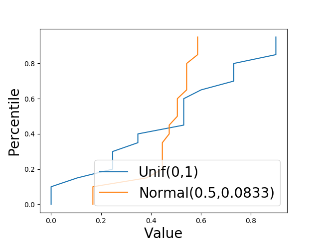
(a) (Non-Private) $\alpha$-Approximate Quantiles for $\alpha=0.1$ and $q\in(0,1)$.

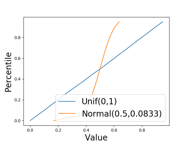
(b) (Non-Private) $\alpha$-Approximate Quantiles for $\alpha=0.0001$ and $q\in(0,1)$.

Figure 2.

3.3. Non-private Quantile Streaming

Lemma 3.6 (GK guarantees (Greenwald and Khanna, 2001)).

Given a data stream $x_{1},\dots,x_{n}$ of elements drawn from $\mathcal{X}$, the GK sketch outputs a list $S(X)$ of $s(=O((1/\alpha)\log(\alpha n)))$ many tuples $(v_{i},g_{i},\Delta_{i})\in(\mathcal{X}\times{\mathbb{N}})\times{\mathbb{N}}\times{\mathbb{N}}$ for $i=1,\dots,s$ such that if $X$ is the data multi-set then

1. $\operatorname*{rank}(X,\operatorname*{val}(v_{i}))\subset[\sum_{j\leq i}g_{j},\Delta_{i}+\sum_{j\leq i}g_{j}]$.

2. $g_{i}+\Delta_{i}\leq 2\alpha n$.

3. The first tuple is $(\min\{x\in X\},1,0)$ and the last tuple is $(\max\{x\allowbreak\in X\},1,0)$.

4. The $v_{i}$ are sorted in ascending order. WLOG, the lower confidence interval bounds $\sum_{j\leq i}g_{j}$ and upper confidence interval bounds $\Delta_{i}+\sum_{j\leq i}g_{j}$ are also sorted in increasing order.

Proof.

The first three statements are part of the GK sketch guarantee. For the third statement, i.e., to see that the $v_{i}$ are sorted in ascending order, we see that the GK sketch construction ensures that $\operatorname*{val}(v_{i})\leq\operatorname*{val}(v_{i+1})$ for all $i$. Since an insertion operation always inserts a repeated value after all previous occurrences and the tuple order is always preserved, it follows that $\operatorname*{ix}(v_{i})\leq\operatorname*{ix}(v_{i+1})$ as well, so in sum $\operatorname*{rank}(X,v_{i})\leq\operatorname*{rank}(X,v_{i+1})$. In other words, the sort order in the GK sketch is stable.

The fact that the sequence $\sum_{j\leq i}g_{j}$ is sorted in increasing order follows from the non-negativity of the $g_{i}$. To ensure that $\Delta_{i}+\sum_{j\leq i}g_{j}$ are sorted in increasing order note that we always have that $\operatorname*{rank}(X,v_{i})\leq\operatorname*{rank}(X,v_{i+1})$ so we can decrement $\Delta_{i}$ and ensure that $\Delta_{i}+\sum_{j\leq i}g_{j}\leq\Delta_{i+1}+\sum_{j\leq i+1}g_{j}$ without violating the guarantees of the GK sketch. ∎

Remark 3.7.

We can add two additional tuples $(-\infty,0,0)$ and $(\infty,0,0)$ to the sketch, which corresponds to respective rank intervals $[0,0]$ and $[n+1,n+1]$. The bounds $g_{i}+\Delta_{i}\leq 2\alpha n$ are preserved. This will ensure that the sets $\{i:\operatorname*{val}(v_{i})<x\}$ and $\{i:\operatorname*{val}(v_{i})>x\}$ for any $x\in\mathcal{X}$ are always non-empty.

4. Differentially Private Algorithms

In this section we present our two DP mechanisms for quantile estimation. Throughout, we assume that $\alpha$ is a user-defined approximation parameter. The goal is to obtain $\alpha$-approximate $q$-quantiles.

The new algorithms we introduce are:

1. $\operatorname*{\texttt{DPExpGKGumb}}$ (Algorithm 2): An exponential mechanism based $(\epsilon,0)$-DP algorithm for computing a single $q$-quantile. To solve the all-quantiles problem with approximation factor $\alpha$, one can run this algorithm iteratively with target quantile $0,\alpha,2\alpha,\dots$. Doing so requires scaling the privacy parameter in each call by an additional $\alpha$ factor which increases the space complexity by a factor of $1/\alpha$. We extend our results to the continual observation setting (Dwork et al., 2010; Chan et al., 2011).

2. $\operatorname*{\texttt{DPHistGK}}$: A histogram based $(\epsilon,0)$-DP algorithm (Algorithm 3) for the $\alpha$-approximate all-quantiles problem. The privacy guarantee of this algorithm is unconditional, but there is no universal theoretical utility bound as in the previous algorithm. However, in some cases the utility is provably better: for example, we show that if the data set is drawn from a normal distribution (with unknown mean and variance), we can avoid the quadractic $1/\alpha^{2}$ factor in the sample complexity that we incur when using $\operatorname*{\texttt{DPExpGKGumb}}$ for the same all-quantiles task.

The rest of the section contains the descriptions of the two algorithms, as well as a detailed theoretical analysis. The next section demonstrates how the histogram-based mechanism can be effectively applied to data generated from a normal distribution.

4.1. $\operatorname*{\texttt{DPExpGKGumb}}$: Exponential Mechanism Based Approach

We first establish how the exponential mechanism and the GK sketch may be used in conjunction to solve the single quantile problem. Concretely, the high level idea is to call the privacy preserving exponential mechanism with a utility function derived from the GK sketch. The exponential mechanism is a fundamental privacy primitive which when given a public set of choices and a private score for each choice outputs a choice that with high probability has a score close to optimal whilst preserving privacy. In the course of constructing our algorithms, we have to resolve two problems; one, how to usefully construct a utility function to pass to the exponential mechanism so that the private value derived is a good approximation to the $q$-quantile, and two, how to execute the exponential mechanism efficiently on the (possibly massive) data universe $\mathcal{X}$. On resolving the first issue we get the (not necessarily efficient) routine Algorithm 1, and on resolving the second issue we get an essentially equivalent but far more efficient routine i.e. Algorithm 2.

Constructing a score function:

We recall that the GK sketch returns a short sequence of elements from the data set with a deterministic confidence interval for their ranks and the promise that for any target quantile $q\in[0,1]$, there is some sketch element that lies within $\alpha n$ units in rank of $\lceil qn\rceil$. One technicality that we run into when trying to construct a score function on the data universe $\mathcal{X}$ is that when a single value occurs with very high frequency in the data set, the ranks of the set of occurrences can span a large interval in $[0,n]$, and there is no one rank we can ascribe to it so as to compare it with the target rank $\lceil qn\rceil$. This can be resolved by defining the score for any data domain value in terms of the distance of its respective rank interval $[r_{\min}(x),r_{\max}(x)]$ (formalized in Definition 3.2) from $\lceil qn\rceil$; elements whose intervals lie closer to the target have a higher score than those whose intervals lie further away.

Efficiently executing the exponential mechanism:

The exponential mechanism samples one of the public choices (in our case some element from the data universe $\mathcal{X}$) with probability that increases with the quality of the choice according to the utility function. In general every element can have a possibly different score and the efficiency of the exponential mechanism can vary widely depending on the context. In our setting, the succinctness of the GK sketch leads to a crucial observation: by defining the score function via the sketch, the data domain is partitioned into a relatively small number of sets such that the utility function is constant on each partition. Concretely, for any two successive elements in the GK sketch, the range of values in the data universe that lie between them will have the same score according to our utility function. We can hence first sample a partition from which to output a value, and then choose a value from within that interval uniformly at random. To make our implementation even more efficient and easy to use, we also make use of the Gumbel-max trick that allows us to iterate through the set of choices instead of storing them in memory.

Outline:

From Definition 4.1 to Lemma 4.3, we formalize how the GK sketch may be used to construct rank interval estimates for any data domain value. We then recall and apply the exponential mechanism with a utility function derived from the GK sketch (Definition 4.4 to Lemma 4.7 and Algorithm 1), and derive the error guarantee Lemma 4.9. We conclude this subsection with a detailed description of an efficient implementation of the exponential mechanism (Algorithm 2 and Lemma 4.10), and summarize our final accuracy and space complexity guarantees in Theorem 4.11.

Definition 4.1.

Let $\hat{r}_{\min}(x)=\max\{\sum_{j\leq i}g_{j}:\operatorname*{val}(v_{i})<x\}$ and $\hat{r}_{\max}(x)=\min\{\Delta_{i}+\sum_{j\leq i}g_{j}:\operatorname*{val}(v_{i})>x\}$. Note that for every $v\in X$ such that $\operatorname*{val}(v)=x$, $\operatorname*{ix}(v)\in[\hat{r}_{\min}(x),\allowbreak\hat{r}_{max}(x)]$.

We formalize the rank interval estimation in a partition-wise manner as below.

Lemma 4.2.

Given a GK sketch $(v_{1},g_{1},\Delta_{1}),\dots,(v_{s},g_{s},\Delta_{s})$, for every $x\in\mathcal{X}$ one of the following two cases holds:

1. $x=v_{i}$ for some $i\in[s]$ and $i=\min\{j:v_{j}=x\}$,

   $$\hat{r}_{\min}(x) =\sum_{j\leq i}g_{j}$$

   $$\hat{r}_{\max}(x) =\min\{\Delta_{i^{*}}+\sum_{j\leq i^{*}}g_{j}:\exists i^{*},\operatorname*{val}(v_{i^{*}})>\operatorname*{val}(v_{i})\}$$

2. $x\in(v_{i-1},v_{i})$, i.e., $x>v_{i-1}$ and $x<v_{i}$ for some $i\in[s]$,

   $$\hat{r}_{\min}(x) =\sum_{j\leq i}g_{j}$$

   $$\hat{r}_{\max}(x) =\Delta_{i+1}+\sum_{j\leq i+1}g_{j}$$

Proof.

Recall that by Remark 3.7 we always have that the first tuple and the last tuple are formal elements at $-\infty$ and $\infty$, ensuring that every data universe element either explicitly occurs in the GK sketch or lies between two values that occur in the GK sketch. Both statements now follow directly from Definition 4.1 and the fact that the values $v_{i}$ occur in increasing order in the sketch (Lemma 3.6). ∎

The quality of the rank interval estimate $[\hat{r}_{\min}(x),\hat{r}_{\max}(x)]$ compared to the true rank interval $[r_{\min}(x),r_{\max}(x)]$ is formalized as follows.

Lemma 4.3.

$|r_{\min}(x)-\hat{r}_{\min}(x)|\leq 2\alpha n$ and $|r_{\max}(x)-\hat{r}_{\max}(x)|\leq 2\alpha n$.

Proof.

Let $i^{*}=\operatorname*{argmax}_{i:\operatorname*{val}(v_{i})<x}\sum_{j\leq i}g_{j}$. Then by Definition of $i^{*}$, we have that $\operatorname*{val}(v_{i^{*}})<x\leq\operatorname*{val}(v_{i^{*}+1})$. It follows that

$$[\operatorname*{ix}(v_{i^{*}}),\operatorname*{ix}(v_{i^{*}+1})] \subset[\sum_{j\leq i^{*}}g_{j},\Delta_{i^{*}+1}+g_{i^{*}+1}+\sum_{j\leq i^{*}}g_{j}]$$

$$\subset[\hat{r}_{\min}(x),\Delta_{i^{*}+1}+g_{i^{*}+1}+\hat{r}_{\min}(x)]$$

Since $r_{\min}(x)\in[\operatorname*{ix}(v_{i^{*}}),\operatorname*{ix}(v_{i^{*}+1})]$ and $g_{i^{*}+1}+\Delta_{i^{*}+1}\leq 2\alpha n$, it follows that $|r_{\min}(x)-\hat{r}_{\min}(x)|\leq 2\alpha n$. The other inequality follows analogously. ∎

Definition 4.4 (Exponential Mechanism (McSherry and Talwar, 2007)).

Let $u:\mathcal{S}^{S}\times\mathcal{R}\rightarrow{\mathbb{R}}$ be an arbitrary utility function with global sensitivity $\Delta_{u}$. For any database summary $d\in\mathcal{S}^{S}$ and privacy parameter $\epsilon>0$, the exponential mechanism $\mathcal{E}_{u}^{\epsilon}:\mathcal{S}^{S}\to\mathcal{R}$ outputs $r\in\mathcal{R}$ with probability $\propto\exp(\frac{\epsilon\cdot u(S(X),r)}{2\Delta_{u}})$ where

$$\Delta_{u}=\max_{X\sim X^{\prime},r}|u(S(X),r)-u(S(X),r)|.$$

The following statement formalizes the trade-off between the privacy parameter $\epsilon$ and the tightness of the tail bound on the score attained by the exponential mechanism.

Theorem 4.5 ( (McSherry and Talwar, 2007; Smith, 2011)).

The exponential mechanism (Definition 4.4) satisfies $\epsilon$-differential privacy. Further, the following tail bound on the utility holds:

$$P\left(u(S(X),\mathcal{E}_{u}^{\epsilon}(S(X)))<\max_{r\in R}u(S(X),r)-\frac{2\Delta_{u}(t+\ln s)}{\epsilon}\right)\leq e^{-t},$$

where $s$ is the size of the universe from which we are sampling from.

To run the exponential mechanism using our approximate rank interval estimates, we define a utility function as follows.

Definition 4.6.

Let $d(\cdot,\cdot)$ denote the $\ell_{1}$ metric on ${\mathbb{R}}$. Given a sketch $S(X)$, we define a utility function on $\mathcal{X}$:

$$u(S(X),x) =-\min\{|y-\lceil qn\rceil|:y\in[\hat{r}_{\min}(x),\hat{r}_{\max}(x)]\}$$

$$=-d(\lceil qn\rceil,[\hat{r}_{\min}(x),\hat{r}_{\max}(x)])$$

The magnitude of the noise that is added in the course of the exponential mechanism depends on the sensitivity of the score function, which we bound from above as follows.

Lemma 4.7.

For all $n>1/\alpha$, the sensitivity of $u$ (i.e., $\Delta_{u}$) is at most $4\alpha n+2$ units.

Proof.

Fix any data set $X^{\prime}$ neighbouring $X$ under swap DP and let $[r^{\prime}_{\min}(\cdot),\allowbreak r^{\prime}_{\max}(\cdot)]$ be the rank ranges with respect to $X^{\prime}$ for values in $\mathcal{X}$. Let $[\hat{r^{\prime}}_{\min}(\cdot),\allowbreak\hat{r^{\prime}}_{\max}(\cdot)]$ denote the confidence interval derived from the GK sketch $S(X^{\prime})$ for values in $\mathcal{X}$.

Claim 4.8.

$|r_{\min}(x)-r^{\prime}_{\min}(x)|\leq 2$, $|r_{\max}(x)-r^{\prime}_{\max}(x)|\leq 2$.

Proof.

These bounds follow directly from the Definition of $r_{\min}$ and $r_{\max}$; under swap DP at most two elements of the stream are changed which implies that the count of the sets defining these terms changes by at most 1 unit each for a total shift of $2$ units (in fact, this can be bounded by $1$ unit). ∎

We now prove the sensitivity bound.

$$u(S(X),x) =-d(\lceil qn\rceil,[\hat{r}_{\min}(x),\hat{r}_{\max}(x)])$$

$$\leq-d(\lceil qn\rceil,[r_{\min}(x),r_{\max}(x)])+2\alpha n$$

$$\leq-d(\lceil qn\rceil,[r^{\prime}_{\min}(x),r^{\prime}_{\max}(x)])+2\alpha n+2$$

$$\leq-d(\lceil qn\rceil,[\hat{r^{\prime}}_{\min}(x),\hat{r^{\prime}}_{\max}(x)])+4\alpha n+2$$

$$\leq u(S(X^{\prime}),x)+4\alpha n+2.$$

Swapping the positions of $X$ and $X^{\prime}$, we get the reverse bound to complete the sensitivity analysis. ∎

Data: $X=(x_{1},x_{2},\ldots,x_{n})$

Input: $\epsilon,\alpha\text{ (approximation parameter)},q\in[0,1]\text{ (quantile parameters)}$, $\Delta_{u}$

1

2$S(X)=\{(v_{i},g_{i},\Delta_{i}):i\in[s]\}\leftarrow GK(X,\alpha)$

3

4Define utility function

(1) $$u(S(X),x)=-\min\{|y-\lceil qn\rceil|:y\in[\hat{r}_{\min}(x),\hat{r}_{\max}(x)]\}.$$

where

$$\hat{r}_{\min}(x) =\max\{\sum_{j\leq i}g_{j}:\operatorname*{val}(v_{i})<x\}$$

$$\hat{r}_{\max}(x) =\min\{\Delta_{i}+\sum_{j\leq i}g_{j}:\operatorname*{val}(v_{i})>x\}$$

5Choose and output $e\in\mathcal{X}$ with probability

$$\propto\exp\left(\frac{\epsilon}{2\Delta_{u}}\cdot u(S(X),e)\right).$$

Algorithm 1 $\operatorname*{\texttt{DPExpGK}}$: Exponential Mechanism DP Quantiles : High Level Description

We can now derive a high probability bound on the utility that is achieved by Algorithm 1.

Lemma 4.9.

If $\hat{x}$ is the value returned $\operatorname*{\texttt{DPExpGK}}$ then with probability $1-\beta$,

$$d(\lceil qn\rceil,[\hat{r}_{\min}(\hat{x}),\hat{r}_{\max}(\hat{x})])\leq 2\alpha n+\frac{2(4\alpha n+2)\log(|\mathcal{X}|/\beta)}{\epsilon}.$$

Proof.

By construction, Algorithm 1 is simply a call to the exponential mechanism with utility function $u(S(X),\cdot)$, Since for any target $q$-quantile, $\lceil qn\rceil$ lies in $[0,n]$ it follows that there is some $i^{*}\in s$ such that $\lceil qn\rceil\in[\sum_{j\leq i^{*}}g_{j},\Delta_{i^{*}+1}+g_{i^{*}+1}+\sum_{j\leq i^{*}}g_{j}]$. It follows that $d(\lceil qn\rceil,[r_{\min}(\operatorname*{val}(v_{i^{*}}),r_{\max}(\operatorname*{val}(v_{i^{*}}))])\leq 2\alpha n$ and that hence $\max(u(S(X),x))\geq-2\alpha n$. If $x^{*}$ is the output of the exponential mechanism, then applying the utility tail bound we get that with probability $1-\beta$,

$$u(S(X),x^{*})\geq-2\alpha n-\frac{2(4\alpha n+2)\log(|\mathcal{X}|/\beta)}{\epsilon}.$$

By definition of $u$, the desired bound follows. ∎

Data: $X=(x_{1},x_{2},\ldots,x_{n})$

Input: $\epsilon,\alpha\text{ (approximation parameter)},q\in[0,1]\text{ (quantile parameters)}$

1 Build summary sketch $S(X)$ and let $s=|S(X)|$.

2 Let $(v_{i},g_{i},\Delta_{i})=S(X)[i]$ for all $i\in[s]$

3 $\text{maxIndex}=-1$

4 $\text{maxValue}=-\infty$

/* Iterating over tuple values $v_{i}$ */

5 Let $i=1$

6 while $i<=s$ do

7       $\hat{r}_{\min}=\sum_{j\leq i}g_{j}$

8       $\hat{r}_{\max}=\min\{\Delta_{i^{*}}+\sum_{j\leq i^{*}}g_{j}:\operatorname*{val}(v_{i^{*}})>\operatorname*{val}(v_{i})\}$

9       $u_{i}=-\min\{|y-\lceil qn\rceil|:y\in[\hat{r}_{\min},\hat{r}_{\max}]\}.$

10       $f=\frac{\epsilon}{2}u_{i}$

11       $\tilde{f}=f+\text{Gumb}(0,1)$

12       if $\tilde{f}>\text{maxValue}$ then

13             $\text{maxIndex}=(i,\mbox{tuple})$

14             $\text{maxValue}=\tilde{f}$

15      $i\leftarrow\min\{j:v_{j}>v_{i}\}$

/* Iterating over intervals between tuples $\mathcal{X}(v_{i-1},v_{i})\subset\mathcal{X}$ */

16 Let $i=1$

17 while $i<=s$ do

18       if $\mathcal{X}(v_{i-1},v_{i})$ is not empty then

19             $\hat{r}_{\min}=\sum_{j\leq i}g_{j}$

20             $\hat{r}_{\max}=\Delta_{i+1}+\sum_{j\leq i+1}g_{j}$

21             $u_{i-1,i}=-\min\{|y-\lceil qn\rceil|:y\in[\hat{r}_{\min},\hat{r}_{\max}]\}.$

22             $f=\log(|\mathcal{X}(v_{i-1},v_{i})|)+\frac{\epsilon}{2}u_{i-1,i}$

23             $\tilde{f}=f+\text{Gumb}(0,1)$

24             if $\tilde{f}>\text{maxValue}$ then

25                   $\text{maxIndex}=(i,\mbox{interval})$

26                   $\text{maxValue}=\tilde{f}$

27            

28      $i\leftarrow i+1$

29if $\text{maxIndex}=(i,\mbox{tuple})$ for some $i\in{1,\dots,s}$ then

30       return $v_{i}$

31 else if $\text{maxIndex}=(i,\mbox{interval})$ for some $i\in{1,\dots,s}$ then

32       Pick $v\in\mathcal{X}(v_{i-1},v_{i})$ uniformly at random

33       return v

34

Algorithm 2 $\operatorname*{\texttt{DPExpGKGumb}}$: Implementing the Exponential Mechanism on $S(X)$ using the Gumbel Distribution

As discussed before, in general a naive implementation of the exponential mechanism as in Algorithm 1 would in general not be efficient. To resolve this issue, in Algorithm 2 we take advantage of the partition of the data domain by the score function and the Gumbel-max trick to implement the exponential mechanism without any higher-order overhead and return an $\alpha$-approximate $q$ quantile. This trick has become a standard way to implement the exponential mechanism over intervals/tuples.

Lemma 4.10.

Algorithm 2 implements the exponential mechanism with utility function $u(S(X),\cdot)$ on the data universe $\mathcal{X}$ with space complexity $O(|S(X)|)$ (where $S(X)$ is the GK sketch) and additional time complexity $O(|S(X)|\log|S(X)|)$.

Proof.

As noted in previous work (Abernethy et al., 2017), if $Z_{1},\ldots,Z_{N}$ are drawn i.i.d. from standard Gumbel distribution,

$$\mathbb{P}\left[f_{i}+Z_{i}=\max_{j\in[N]}\{f_{j}+Z_{j}\}\right]=\frac{\exp(f_{i})}{\sum_{j\in[N]}\exp(f_{j})},\forall i\in[N].$$

We recall that when running the exponential mechanism on $\mathcal{X}$, we want to sample the element $x\in\mathcal{X}$ with probability $\propto\exp(\epsilon u(S(X),x)$. To implement the exponential mechanism via the identification with Gumbel $\operatorname*{argmax}$ distribution above, we will simply compute the scores $u(S(X),x)$ and let $f_{i}=\epsilon\cdot u(S(X),x)$.

For $x\in\mathcal{X}$ such that $x=v_{i}$ for some $i\in[s]$, Algorithm 2 directly computes the scores according to Definition 4.6 and Lemma 4.2; this is formalized by lines 2 to 2 in the pseudo code.

For $x\in\mathcal{X}$ which lie strictly between the tuple values $\{v_{i}:i\in[s]\}$, we proceed as follows. Fixing $i$, from Lemma 4.2 we have that that for $\mathcal{X}(v_{i-1},v_{i}):=\{x\in\mathcal{X}:x>v_{i-1},x<v_{i}\}$, the rank confidence interval estimate is the same, i.e. $[\sum_{j\leq i-1}g_{j},\Delta_{i}+\sum_{j\leq i}g_{j}]$. It follows from Definition 4.6 that for all such domain values the the utility function score $u(S(X),\cdot)$ is equal; this is denoted $u_{i-1,i}$ in the pseudo code. By summing the probabilities for sampling individual domain elements, it follows that the likelihood of the exponential mechanism outputting some value from the set $\mathcal{X}(v_{i-1},v_{i})$ is $\propto|\mathcal{X}(v_{i-1},v_{i})|\exp(\epsilon u_{i-1,i}/2)=\exp(\epsilon u_{i-1,i}/2+\log(|\mathcal{X}(v_{i-1},v_{i})|))$. This is formalized by lines 2 to 2 in the pseudo code.

Finally, if some interval is selected, then by outputting elements chosen uniformly at random, we ensure that the likelihood of $x\in\mathcal{X}(v_{i-1},v_{i})$ being output is $\propto\frac{1}{|\mathcal{X}(v_{i-1},v_{i})|}\cdot\exp(\epsilon u_{i-1,i}/2+\log(|\mathcal{X}(v_{i-1},v_{i})|)=\exp(\epsilon u_{i-1,i})$. Note that we do not need to account for ties in the Gumbel scores as the event $f_{i}+Z_{i}=f_{j}+Z_{j}$ for any $j\not=i$ has measure $0$.

To bound the space and time complexity; we note that by the guarantees of the GK sketch, the size of the sketch $S(X)$ is $O((1/\alpha)\allowbreak\log\alpha n)$; we compute Gumbel scores by iterating over tuples and intervals of which there are at most $O(S(X))$-many of each, each computation takes at most $O(\log|S(X)|)$ time, and only the max score and index seen at any point is tracked in the course of the algorithm. ∎

We can now state and prove our main theorem in this section, proving utility bounds for $\alpha$-approximating quantiles through $\operatorname*{\texttt{DPExpGK}}$ with sublinear space.

Theorem 4.11.

Algorithm 2 is $\epsilon$-differentially private. Let $\hat{x}$ be the value returned by Algorithm 2 when initialized with target quantile $q$. The following statements hold:

1. Algorithm 2 can be run with space complexity $O(1/\alpha\log\alpha n)$, such that with probability $1-\beta$

   (2) $$d(\lceil qn\rceil,[\hat{r}_{\min}(\hat{x}),\hat{r}_{\max}(\hat{x})])\leq 2\alpha n+\frac{2(4\alpha n+2)\log(|\mathcal{X}|/\beta)}{\epsilon}$$

2. For $n>\frac{\log|\mathcal{X}|/\beta}{12\alpha\epsilon}$, Algorithm 2 can be run with space complexity $O\left((\alpha\epsilon)^{-1}\log(|\mathcal{X}|/\beta)\log(\alpha\epsilon n)\right)$ such that with probability $1-\beta$, $\hat{x}$ is an $\alpha$ approximate $q$-quantile.

Our dependence in $\alpha$, which for practical purposes is usually the most important term, is optimal. Very recent subsequent work by Kaplan and Stemmer (Kaplan and Stemmer, 2021) shows how to improve the dependence in other parameters if approximate (rather than pure) differential privacy is allowed, or if the stream length is large enough.

Proof.

The privacy guarantee of Algorithm 2 follows from the privacy guarantee of the exponential mechanism and Lemma 4.10. The accuracy bound in equation 2 is simply a restatement of Lemma 4.9. To derive the second statement, we substitute $\frac{\alpha\min\{\epsilon,1\}}{24\log(|\mathcal{X}|/\beta)}$ for the approximation parameter $\alpha$ in equation 2 and get

$$d(\lceil qn\rceil,[\hat{r}_{\min}(\hat{x}),\hat{r}_{\max}(\hat{x})])$$

$$\leq 2\cdot\frac{\alpha\min\{\epsilon,1\}n}{24\log(|\mathcal{X}|/\beta)}+\frac{2(4(\frac{\alpha\min\{\epsilon,1\}}{24\log(|\mathcal{X}|/\beta)})n+2)\log(|\mathcal{X}|/\beta)}{\epsilon}$$

$$\leq\frac{\alpha n}{12\log(|\mathcal{X}|/\beta)}+\frac{\alpha n}{3}+\frac{4\log|\mathcal{X}|/\beta}{\epsilon}$$

$$\leq\frac{\alpha n}{12}+\frac{\alpha n}{3}+\frac{\alpha n}{3}$$

$$\leq\alpha n.$$

The space complexity bound now follows directly from the space complexity bound derived in Lemma 4.10, the space complexity bound $O(1/\alpha\log\alpha n)$ for the GK sketch, and by substituting
$\frac{\alpha\min\{\epsilon,1\}}{24\log(|\mathcal{X}|/\beta)}$ for $\alpha$. ∎

4.2. $\operatorname*{\texttt{DPHistGK}}$: Histogram Based Approach

For methods in this section, we assume that we have $K\geq 1$ disjoint bins each of width $w$ (e.g., $w=\alpha/2$). These bins are used to construct a histogram.

Essentially, Algorithm 3 builds an empirical histogram based on the GK sketch, adds noise so that the bin values satisfy $(\epsilon,0)$-DP, and converts this empirical histogram to an approximate empirical CDF, from which the quantiles can be approximately calculated.

Data: $X=(x_{1},x_{2},\ldots,x_{n})$

Input: $\epsilon,\alpha\text{ (approximation parameter)},q\in[0,1]\text{ (quantile parameters)},w$

1

2Build summary sketch $S(X)$ where

3 $S(X)=\{(v_{i},g_{i},\Delta_{i}):i\in[s]\}\leftarrow GK(X,\alpha)$

4

/* cell labels $a_{i}$ and counts $c_{i}=0$ */

5 Initialize data-agnostic (empty) histogram $Hist=\langle(a_{i},c_{i}),\ldots\rangle$ with cell widths $w$

6for $(v_{i},g_{i},\Delta_{i})\in S(X)$ do

7       Insert $g_{i}$ counts of $v_{i}$ into histogram $Hist$

8$c=0$

9 $H=[]$

10 for $(a_{i},c_{i})\in Hist$ do

11       $\tilde{c}_{i}=\max(0,c_{i}+\operatorname*{Lap}(0,2/\epsilon))$

12      Append $(a_{i},c+\tilde{c}_{i})$ to $H$

13      $c=c+\tilde{c}_{i}$

14

15$r=\lceil q\cdot n\rceil$

16for $(b,rank)\in H$ do

17       if $r<rank$ then

18             return $b$

19      

20

/* return last element of $H$ */

21

22return $H[|H|-1]$

Algorithm 3 $\operatorname*{\texttt{DPHistGK}}$: Computing DP Quantiles in Bounded Space

Lemma 4.12.

Algorithm 3 satisfies $(\epsilon,0)$-DP.

Proof.

For any $i\in[n]$, any item $x_{i}$ can belong in at most one bin. Plus, the global sensitivity of the function that computes the empirical histogram is $2$, since changing a single item can change the contents of at most two bins.

As a result, adding noise of $\operatorname*{Lap}(0,2/\epsilon)$ to each bin satisfies $\epsilon$-DP by Theorem 4.13. ∎

Theorem 4.13 (Laplace Mechanism (Dwork et al., 2006)).

Fix $\epsilon>0$ and any function $f:\mathcal{Y}^{n}\rightarrow{\mathbb{R}}^{K}$. The Laplace mechanism outputs

$$f(y)+(L_{1},\ldots,L_{K}),$$

$L_{1},\ldots,L_{K}\sim\operatorname*{Lap}(0,GS_{f}/\epsilon)$ where $GS_{f}$ is the global sensitivity of the function $f$. Furthermore, the mechanism satisfies $(\epsilon,0)$-DP.

5. Learning differentially private quantiles of a normal distribution with unknown mean

We demonstrate one use case of $\operatorname*{\texttt{DPHistGK}}$ where the space complexity required improves upon the worst-case bound for $\operatorname*{\texttt{DPExpGK}}$, Theorem 4.11. While the histogram based mechanism does not have universal utility bounds in the spirit of the above theorem, the results in this section serve as one simple example where it may yield desirable accuracy while using less space.

Suppose that we are given an i.i.d. sample $S=(X_{1},X_{2},\ldots,X_{n})$ such that for all $i\in[n]$, $X_{i}\sim\mathcal{N}(\mu,\sigma^{2}I_{d\times d})$, $\mu\in{\mathbb{R}}^{d}$. The goal is to estimate DP quantiles of the distribution $\mathcal{N}(\mu,\sigma^{2}I_{d\times d})$ without knowledge of $\mu$ or $\sigma^{2}$. We will show how to estimate the quantiles assuming that $\sigma^{2}$ is known. Note that it is easy to generalize the work to the case where $\sigma^{2}$ is unknown as follows:

For any sample $S$ drawn from i.i.d. from $\mathcal{N}(\mu,\sigma^{2}I_{d\times d})$, the $1-\beta$ confidence interval is

$$\bar{X}\pm\frac{\sigma}{\sqrt{n}}\cdot z_{1-\beta/2},$$

where $z_{1-\beta/2}$ is the $1-\beta/2$ quantile of the standard normal distribution and $\bar{X}$ is the empirical mean. The length of this interval is fixed and equal to

$$\frac{2\sigma z_{1-\beta/2}}{\sqrt{n}}=\Theta\left(\frac{\sigma}{\sqrt{n}}\sqrt{\log\frac{1}{\beta}}\right).$$

In the case where $\sigma^{2}$ is unknown, the confidence interval becomes

$$\bar{X}\pm\frac{s}{\sqrt{n}}\cdot t_{n-1,1-\beta/2},$$

where $s^{2}=\frac{1}{n-1}\sum_{i=1}^{n}(X_{i}-\bar{X})^{2}$ is the sample variance (sample estimate of $\sigma^{2}$) and $t_{n-1,1-\beta/2}$ is the $1-\beta/2$ quantile of the $t$-distribution with $n-1$ degrees of freedom. The length of the interval can be shown to be

$$\frac{2\sigma}{\sqrt{n}}\cdot k_{n}\cdot t_{n-1,1-\beta/2}=\Theta\left(\frac{\sigma}{\sqrt{n}}\sqrt{\log\frac{1}{\beta}}\right),$$

where $k_{n}=1-O(1/n)$ is an appropriately chosen constant. See (Lehmann and Romano, 2005; Karwa and Vadhan, 2017; Keener, 2010) for more details and discussion. We will assume that $\sigma^{2}$ is known and proceed to show sample and space complexity bounds. One could also estimate the variance in a DP way and then prove the complexity bounds.

For any $q\in(0,1)$, we denote the $q$-quantile of the sample as $Q_{S}^{q}$ and the $q$-quantile of the distribution as $Q_{\mathcal{D}}^{q}$.

That is, for any $q\in(0,1)$ and sample $S=(X_{1},X_{2},\ldots,X_{n})$, we wish to obtain a DP $q$-quantile $\tilde{Q}_{S}^{q}$ with the following guarantee:

$$\mathbb{P}[\mathopen{\|}Q_{\mathcal{D}}^{q}-\tilde{Q}_{S}^{q}\mathclose{\|}\geq\alpha]\leq\beta,$$

for any $\beta\in(0,1],\alpha>0$.

We shall proceed to use a three-step approach: (1) Estimate a DP range of the population in sub-linear space; (2) Use this range of the population to construct a DP histogram using the stream $S$; (3) Use the DP histogram to estimate one or more quantiles via the sub-linear data structure of Greenwald and Khanna.

In the case where $d=1$, by Theorem 5.1, there exists an $(\epsilon,\delta)$-DP algorithm $\tilde{Q}_{S}^{q}$ such that if $\mu\in(-R,R)$ then using space of $O(\max\{\frac{R}{\sigma},\frac{1}{\alpha}\log\alpha n\})$ (with probability 1) as long as the stream length is at least

$$n\geq O\bigg{(}\max\bigg{\{}\min\bigg{\{} O\left(\frac{R}{\epsilon\sigma\alpha}\log\frac{R}{\sigma\beta}\right),O\left(\frac{R}{\epsilon\sigma\alpha}\log\frac{1}{\beta\delta}\right)\bigg{\}},$$

$$O\left(\frac{R^{2}}{\sigma^{2}\alpha^{2}}\log\frac{1}{\beta}\right)\bigg{\}}\bigg{)},$$

we get the guarantee that, for all $\beta\in(0,1],\alpha>0$,

$$\mathbb{P}[\mathopen{\|}Q_{\mathcal{D}}^{q}-\tilde{Q}_{S}^{q}\mathclose{\|}\geq\alpha]\leq\beta.$$

Intuitively, this means that: (1) Space: We need less space to estimate any quantile with DP guarantees if the distribution is less concentrated (i.e., $\sigma$ can be large) or if we do not require a high degree of accuracy for our queries (i.e., $\alpha$ can be large). (2) Stream Length: We need a large stream length to estimate quantiles if we require a high degree of accuracy (i.e., smaller $\beta,\alpha$), or do not have a good public estimate of $\mu$ (large $R$), or have small privacy parameters (small $\epsilon,\delta$), or have concentrated datasets (small $\sigma$).

Theorem 5.1.

For the 1-D normal distribution $\mathcal{N}(\mu,\sigma^{2})$, let $S=(X_{1},X_{2},\ldots,X_{n})$ be a data stream through which we wish to obtain $\tilde{Q}_{S}^{q}$, a DP estimate of the $q$-quantile of the distribution.

For any $q\in(0,1)$, there exists an $(\epsilon,\delta)$-DP algorithm such that, with probability at least $1-\beta$, we obtain $|Q_{\mathcal{D}}^{q}-\tilde{Q}_{S}^{q}|\leq\alpha$ for any $\alpha>0$, $\beta\in(0,1],\epsilon,\delta\in(0,1/n)$ and for stream length

$$n\geq\max\left\{\min\left\{A,B\right\},C\right\},\ \ \text{where}$$

$$A=O\left(\frac{R}{\epsilon\sigma\alpha}\log\frac{R}{\sigma\beta}\right),B=O\left(\frac{R}{\epsilon\sigma\alpha}\log\frac{1}{\beta\delta}\right),C=O\left(\frac{R^{2}}{\sigma^{2}\alpha^{2}}\log\frac{1}{\beta}\right)$$

as long as $\mu\in(-R,R)$ and using space of $O(\max\{\frac{R}{\sigma},\frac{1}{\alpha}\log\alpha n\})$.

Proof.

For any stream $S=(X_{1},\ldots,X_{n})$, we use the triangle inequality so that

(3) $$|Q_{\mathcal{D}}^{q}-\tilde{Q}_{S}^{q}| \leq|Q_{\mathcal{D}}^{q}-Q_{S}^{q}|+|Q_{S}^{q}-\tilde{Q}_{S}^{q}|$$

(4) $$\leq\alpha/2+\alpha/2.$$

$|Q_{\mathcal{D}}^{q}-Q_{S}^{q}|\leq\alpha/2$ follows with probability $1-\beta/2$ by Corollary 5.3 and $|Q_{S}^{q}-\tilde{Q}_{S}^{q}|\leq\alpha/2$ follows with probability $1-\beta/2$ by Lemma 5.4. The space complexity follows with probability 1 via the deterministic nature of the Greenwald-Khanna sketch. ∎

Lemma 5.2 (Dvoretzky-Kiefer-Wolfowitz inequality (Dvoretzky et al., 1956)).

For any $n\in\mathbb{Z}_{+}$, let $X_{1},\ldots,X_{n}$ be i.i.d. random variables with cumulative distribution function $F$ so that $F(x)$ is the probability that a single random variable $X$ is less than $x$ for any $x\in{\mathbb{R}}$. Let the corresponding empirical distribution function be $F_{n}(x)=\frac{1}{n}\sum_{i=1}^{n}\mathds{1}[X_{i}\leq x]$ for any $x\in{\mathbb{R}}$. Then for any $\gamma>0$,

$$\mathbb{P}\left(\sup_{x\in{\mathbb{R}}}|F_{n}(x)-F(x)|>\gamma\right)\leq 2\exp(-2n\gamma^{2}).$$

Corollary 5.3.

For any $q\in(0,1)$, let $Q_{\mathcal{D}}^{q}$ be the $q$-quantile estimate for the distribution $\mathcal{D}$ and $Q_{S}^{q}$ be the $q$-quantile estimate for the sample. Then, $|Q_{\mathcal{D}}^{q}-Q_{S}^{q}|\leq\alpha/2$ with probability $1-\beta/2$ when $n\geq\frac{2}{\alpha^{2}}\log 4/\beta$.

Proof.

Follows by the DKW inequality (Lemma 5.2) where $n\geq\frac{1}{2\gamma^{2}}\log 4/\beta$ and $\gamma=\alpha/2$. ∎

Lemma 5.4.

For any $q\in(0,1)$, $\alpha>0$, $\beta\in(0,1]$, $\epsilon,\delta\in(0,1/n)$, there exists an $(\epsilon,\delta)$-differentially private algorithm $\tilde{Q}_{S}^{q}$ for computing the $q$-quantile such that

$$|Q_{S}^{q}-\tilde{Q}_{S}^{q}|\leq\alpha/2,$$

with probability $\geq 1-\beta$ for stream length

$$n\geq O\left(\min\{O\left(\frac{R}{\epsilon\sigma\alpha}\log\frac{R}{\sigma\beta}\right),O\left(\frac{R}{\epsilon\sigma\alpha}\log\frac{1}{\beta\delta}\right)\}\right).$$

Furthermore, with probability 1, $\tilde{Q}_{S}^{q}$ uses space of $O(\max\{\frac{R}{\sigma},\frac{1}{\alpha}\log\alpha n\})$.

Proof.

First, by the tail bounds of the Gaussian distribution (Claim 5.6), we can obtain that for any $i\in[n]$,

$$\mathbb{P}[|X_{i}-\mu|>c]\leq 2e^{-c^{2}/2\sigma^{2}},$$

so that by the union bound,

$$\mathbb{P}[\exists i,|X_{i}-\mu|\geq c]\leq 2ne^{-c^{2}/2\sigma^{2}},$$

which implies that for any $\beta\in(0,1]$,

$$\mathbb{P}[\forall i,|X_{i}-\mu|\leq\sigma\sqrt{2\log 4n/\beta}]\geq 1-\beta/2,$$

which holds by our sample complexity (stream length) guarantees.

Next, let $r=\lceil R/\sigma\rceil$. Divide $[-R-\sigma/2,R+\sigma/2]$ into $2r+1$ bins of length at most $\sigma$ each. Each bin $B_{j}$ should equal $((j-0.5)\sigma,(j+0.5)\sigma]$ for any $j\in\{-r,\ldots,r\}$. Next run the histogram learner of Lemma 5.5 with per-bin accuracy parameter of $\alpha/K$, high-probability parameter of $\beta/2$, privacy parameters $\epsilon,\delta\in(0,1/n)$, and number of bins $K=2\lceil R/\sigma\rceil+1$. We can do this because of our sample complexity (stream length) bounds. Then we obtain noisy estimates $\tilde{p}_{-r},\ldots,\tilde{p}_{r}$ with per-bin accuracy of $\alpha/K$. Then any quantile estimate would have accuracy of $\alpha$ (by summing noisy estimates for at most $K$ bins).

Next, we use these bins to construct a sketch (private by DP post-processing) based on the deterministic algorithms of (Greenwald and Khanna, 2004) to, with probability 1, obtain space of $O(\max\{\frac{R}{\sigma},\frac{1}{\alpha}\log\alpha n\})$. ∎

Lemma 5.5 (Histogram Learner (Bun et al., 2015; Vadhan, 2017; Karwa and Vadhan, 2017)).

For every $K\in\mathbb{N}\cup\{\infty\}$ and every collection of disjoint bins $B_{1},\ldots,B_{K}$ defined on the domain $\mathcal{X}$. For any $n\in\mathbb{N}$, $\epsilon,\delta\in(0,1/n),\alpha>0,$ and $\beta\in(0,1)$, there exists an $(\epsilon,\delta)$-DP algorithm $M:\mathcal{X}^{n}\rightarrow{\mathbb{R}}^{K}$ such that for every distribution $\mathbb{D}$ on the domain $\mathcal{X}$, if

1. $X_{1},\ldots,X_{n}\sim\mathbb{D}$, $p_{k}=\mathbb{P}[X_{i}\in B_{k}]$ for any $k\in[K]$,

2. $(\tilde{p}_{1},\ldots,\tilde{p}_{K})\leftarrow M(X_{1},\ldots,X_{n})$,

3. $n\geq\max\left\{\min\left\{\frac{8}{\epsilon\alpha}\log\frac{2K}{\beta},\frac{8}{\epsilon\alpha}\log\frac{4}{\beta\delta}\right\},\frac{1}{2\alpha^{2}}\log\frac{4}{\beta}\right\}$,

then (over the randomness of the data $X_{1},\ldots,X_{n}$ and of $M$)

1. $\mathbb{P}_{\underline{X}\sim\mathbb{D},M}[|\tilde{p}_{k}-p_{k}|\leq\alpha]\geq 1-\beta$,

2. $\mathbb{P}[\operatorname*{argmax}_{k}\tilde{p}_{k}=j]\leq np_{j}$ if $K\geq 2/\delta$,

3. $\mathbb{P}[\operatorname*{argmax}_{k}\tilde{p}_{k}=j]\leq np_{j}+2\exp(-(\epsilon n/8)\cdot(\max_{k}p_{k}))$ if $K<2/\delta$.

Claim 5.6 (Gaussian Tail Bound).

Let $Z$ be a random variable distributed according to a standard normal distribution (with mean 0 and variance 1). For every $t>0$,

$$\mathbb{P}[|Z|>t]\leq 2\exp(-t^{2}/2).$$

6. Continual Observation

We now describe how our one-shot approach can be used as a black box to obtain a continual observation solution (Dwork et al., 2010; Chan et al., 2011).

Data: Input stream $X=(x_{1},\dots,x_{n})$ for some $n>n_{\min}=\Omega\left(\frac{1}{\epsilon\alpha^{2}}\log^{2}n\log\left(\frac{|\mathcal{X}|\log n}{\alpha\beta}\right)\right)$, privacy parameter $\epsilon$, approximation parameter $\alpha$, target quantile $q$

1 Let $s=0$

2 $\epsilon^{*}\leftarrow O(\alpha\epsilon/\log n)$

3 $\alpha^{*}\leftarrow\alpha/2$

$\mathrm{cp}(s)\leftarrow n_{\min}$ /* stores stream checkpoints */

4 Instantiate $\mathrm{GK}\leftarrow GK(\alpha^{*})$

$v_{s}\leftarrow\perp$ /* holds $\alpha$-approximate $q$-quantile */

5 for stream element $x_{s}\in X$ do

6       $s\leftarrow s+1$

7       $\mathrm{GK}.insert(x_{s})$

8       if $s=\lceil\mathrm{cp}(s-1)\rceil$ then

9             $v_{s}\leftarrow\operatorname*{\texttt{DPExpGK}}(\mathrm{GK},\epsilon^{*},\alpha^{*},q)$

10             $\mathrm{cp}(s)\leftarrow\mathrm{cp}({s-1})(1+\alpha/2)$

11            

12       else

13             $v_{s}\leftarrow v_{s-1}$

14             $\mathrm{cp}(s)\leftarrow\mathrm{cp}({s-1})$

15            

16      

Algorithm 4 Continual Observation DP Quantiles

Lemma 6.1.

If $x\in X$ is an $\alpha/2$-approximate $q$-quantile for a data set $X$ (for some $q\in[0,1]$), then it is an $\alpha$-approximate $q$-quantile for any data set $X^{\prime}\supset X$ such that $|X^{\prime}|\leq(1+\alpha/2)|X|$.

Proof.

Since $x$ is an $\alpha/2$-approximate $q$-quantile, we have that

$$(1-\alpha/2)|X|\leq\operatorname*{rank}_{X}(x)\leq(1+\alpha/2)|X|.$$

We then have that

$$\operatorname*{rank}_{X^{\prime}}(x) =\sum_{y\in X^{\prime}}\mathds{1}[y\leq x]$$

$$=\sum_{y\in X}\mathds{1}[y\leq x]+\sum_{y\in X^{\prime}\backslash X}\mathds{1}[y\leq x]$$

$$\Rightarrow\sum_{y\in X}\mathds{1}[y\leq x] \leq\sum_{y\in X^{\prime}}\mathds{1}[y\leq x]\leq\sum_{y\in X}\mathds{1}[y\leq x]+\sum_{y\in X^{\prime}\backslash X}\mathds{1}[y\leq x]$$

$$\Rightarrow(1-\alpha/2)|X| \leq\sum_{y\in X^{\prime}}\mathds{1}[y\leq x]\leq(1+\alpha/2)|X|+(|X^{\prime}|-|X|)$$

$$\Rightarrow(1-\alpha/2)|X| \leq\sum_{y\in X^{\prime}}\mathds{1}[y\leq x]\leq(1+\alpha/2)|X|+\alpha|X|/2$$

$$\Rightarrow(1-\alpha)|X| \leq\sum_{y\in X^{\prime}}\mathds{1}[y\leq x]\leq(1+\alpha)|X|,$$

i.e., $x$ is also an $\alpha$-approximate $q$-quantile for $X^{\prime}$, as required. ∎

Lemma 6.2.

For any $\beta\in(0,1]$, with probability $\geq 1-\beta$, for all $s\in\{\mathrm{cp}(s^{\prime}):s^{\prime}\in[n]\}$, $v_{s}$ is an $\alpha/2$-approx. $q$-quantile for $X[1:s]$.

Proof.

First we bound the size of the set of checkpoints $\{\mathrm{cp}(s^{\prime}):s^{\prime}\in[n]\}$. Since a new checkpoint value is generated only when $s\geq(1+\alpha/2)\mathrm{cp}(s-1)$, it follows that for any new checkpoint where $\mathrm{cp}(s^{\prime})\neq\mathrm{cp}(s^{\prime}-1)$, we have $\mathrm{cp}(s^{\prime})\geq(1+\alpha/2)\mathrm{cp}(s^{\prime}-1)$. Using Theorem 4.11, we set the first checkpoint value to $\frac{\log|\mathcal{X}|/\beta}{12\alpha^{*}\epsilon^{*}}$. As a result, there are at most $k\leq\log_{1+\alpha/2}n=O(\frac{1}{\alpha}\log n)$ checkpoints using the fact that for all $x>-1$, $\frac{x}{1+x}\leq\log(1+x)\leq x$.

Since $v_{\mathrm{cp}(s)}$ is the output of $\operatorname*{\texttt{DPExpGK}}$ given a GK sketch with accuracy parameter $\alpha^{*}$ and privacy parameter $\epsilon^{*}$ it follows that with probability $1-\beta^{*}$ where $\beta^{*}=O(\alpha\beta/\log n)$, $\operatorname*{rank}_{X[1:s^{\prime}]}\in(1-\alpha/2,1+\alpha/2)qn$. The stated result follows by applying the union bound over all private approximate quantile computations at checkpoints. ∎

Theorem 6.3.

Let $\epsilon,\alpha>0$, $n\in{\mathbb{Z}}$. For any $\beta\in(0,1]$, with probability $\geq 1-\beta$, Algorithm 4 maintains an $\alpha$-approximate $q$-quantile at every point $s$ in the data stream $s=\Omega\left(\frac{1}{\epsilon\alpha^{2}}\log^{2}n\log\left(\frac{|\mathcal{X}|\log n}{\alpha\beta}\right)\right)$. Furthermore, Algorithm 4 satisfies $\epsilon$-DP.

Proof.

To see that Algorithm 4 is $\epsilon$-DP, we observe that the output of this algorithm throughout the data stream can be summarized by its outputs at the checkpoints $\{\mathrm{cp}(s):s\in[n]\}$ (the points in the stream at which a new checkpoint is reached and a new value released are known publicly, so this suffices for privacy analysis). It follows that there is a choice of $\epsilon^{*}=\Omega(\alpha\epsilon/\log n)$ that gives us an $\epsilon$-DP mechanism.

We now prove the accuracy guarantee. For any arbitrary $s\geq\frac{\log|\mathcal{X}|/\beta}{12\alpha^{*}\epsilon^{*}}$, i.e., the default checkpoint value, the output $v_{s}$ of the algorithm will equal the value at the most recent checkpoint, i.e., $v_{\mathrm{cp}(s)}$. Then, since $|X[1:s]|=s\leq(1+\alpha/2)\mathrm{cp}(s)\leq(1+\alpha/2)|X[1:\mathrm{cp}(s)]|$, by Lemma 6.1 it follows that $\operatorname*{rank}_{X[1:s]}(v_{s})\in(1-\alpha,1+\alpha)qn$, i.e., $v_{s}$ is an $\alpha$-approximate $q$-quantile for $X[1:s]$. ∎

We conclude by mentioning that our continual observation solution incurs roughly a $O(\log n/\alpha)$ overhead in the space complexity, which is in line with classical works in differential privacy and adversarially robust streaming (Ben-Eliezer et al., 2020; Dwork et al., 2010). Concurrently, Stemmer and Kaplan (Kaplan and Stemmer, 2021) developed a notion of streaming sanitizers which yields a continual observation guarantee “for free”, without incurring such an overhead over the one-shot case.

7. Experimental Evaluation

In this section, we experimentally evaluate our sublinear-space exponential-based mechanism, $\operatorname*{\texttt{DPExpGKGumb}}$. We study how well our algorithm performs in terms of accuracy and space usage. Note that we proved space complexity and accuracy bounds for the algorithm; part of this section validates that the space complexity of the algorithm is indeed very small in practice, and that the accuracy is typically closely tied to the approximation parameter $\alpha$.

Our main baselines will be $\operatorname*{\texttt{DPExpFull}}$ (without use of the GK sketch but with the use of DP) and the true quantile value. The true quantile values are used to compute relative error, the absolute value of the difference between the estimated quantile and the true quantile, divided by the standard deviation of the data set.

$\operatorname*{\texttt{DPExpFull}}$

The use of the exponential mechanism to $\epsilon$-privately compute $q$-quantiles without the use of the sketching data structure. The space used by this algorithm is of order $\Theta(n)$. See Section 7.3 for further implementation details. We experimentally validate $\operatorname*{\texttt{DPExpGKGumb}}$ varying the following parameters: $\epsilon>0$ (the privacy parameter), $n$ (the stream length), and $\alpha$ (the approximation parameter). We show results on both synthetically-generated datasets and time-series real-world datasets.

The real-world time-series datasets (Dua and Graff, 2017) are: (1) Taxi Service Trajectory: A dataset from the UCI machine learning repository describing trajectories performed by all 442 taxis (at the time) in the city of Porto in Portugal (Moreira-Matias et al., 2013). This dataset contains real-valued attributes with about 1.5 million instances. (2) Gas Sensor Dataset: A UCI repository dataset containing recordings of 16 chemical sensors exposed to varying concentrations of two gas mixtures (Fonollosa et al., 2015). The sensor measurements are acquired continuously during a 12-hour time range and contains about 4 millions instances.

7.1. Synthetic Datasets

In this section, we compare our methods on synthetically generated datasets. We vary the following parameters:

1. Privacy Parameter $\epsilon$: For each choice of $\epsilon\geq 0$, we run the DP algorithms over 100 trials and output means and confidence intervals over these trials.

2. Stream Length $n$: The size of the stream $x_{1},\ldots,x_{n}$ received by the sketching algorithm. When we vary $n$, we fix $\epsilon=1$.

3. Approximation Parameter $\alpha$: The approximation factor used by the internal GK sketch in our solution.

4. Data Distribution: We generate data from uniform and Gaussian distributions. We use a uniform distribution in range $[0,1]$ (i.e., $U(0,1)$) or a normal distribution with mean $0$ and variance $1$ (i.e., $N(0,1)$), clipped to the interval $[-10,10]$.

We show results on space usage and relative error (both plotted mostly on logarithmic scales) from non-DP estimates, as we vary the parameters listed above. Here, the relative error is the absolute difference between the DP estimate and the true non-DP quantile value divided by the standard deviation of the data set. For plots that compare the relative error to the stream length (e.g., Figures 3(a) and 4(a)), the relative error are on the y-axis while the stream length or the privacy parameter are on the x-axis. For plots that compare the data structure size to the stream length (e.g., Figures 3(b) and 4(b)), the sizes are on the y-axis while the stream length is be on the x-axis. We graph the mean relative error over 100 trials of the exponential mechanism per experiment, as well as the $80\%$ confidence interval computed by taking the $10$th and $90$th percentile. While the quantile to be estimated can also be varied, we fix it to $q=0.5$ (the median) throughout as the relative error and the space usage generally do not seem to vary much with choice of $q$.

In Figures 3 and 4 we vary the stream length $n$ for an approximation factor of $\alpha=10^{-4}$. The streams are either normally or uniformly distributed. In Figures 3(a) and 3(b), we compare $\operatorname*{\texttt{DPExpGKGumb}}$ (space strongly sublinear in $n$) vs. $\operatorname*{\texttt{DPExpFull}}$ (uses space of $O(n)$) in terms of space usage and accuracy. We verify experimentally that $\operatorname*{\texttt{DPExpFull}}$ will use more space than $\operatorname*{\texttt{DPExpGKGumb}}$. On the other hand, the space savings incurred by $\operatorname*{\texttt{DPExpGKGumb}}$ are expected to create some drop in accuracy; recall that such a drop must occur even for non-private streaming algorithms. Figures 4(a) and 4(b) the streams are from a normal distribution instead of uniform.

In general we find that although our method $\operatorname*{\texttt{DPExpGKGumb}}$ incurs higher error, in absolute terms it remains quite small and the $95\%$ confidence intervals tend to be adjacent for $\operatorname*{\texttt{DPExpGKGumb}}$ and $\operatorname*{\texttt{DPExpFull}}$. However, there is a clear trend of an exponential gap developing between their respective space usages which is a natural consequence of the space complexity guarantee of the GK sketch. This holds for both distributions studied (Figures 3 and Figure 4).

In Figures 6 and 7, we vary the stream length for a relatively large approximation factor of 0.1. Here we see that compared to the non-approximate method we incur far higher error, although there is also a concomitant increase in the space savings. This is not a typical use-case since the non-private error can itself be large, but we get a complete picture of how space usage and performance vary with this user-defined parameter.

(a) Mean relative error and 80% confidence interval vs. stream length over $100$ trials

(b) Data structure sizes vs. stream length

Figure 3. $\operatorname*{\texttt{DPExpGKGumb}}$ versus $\operatorname*{\texttt{DPExpFull}}$ for uniformly random data, $\alpha=10^{-4}$, $\epsilon=1$, $q=0.5$

(a) Mean relative error and 80% confidence interval vs. stream length over $100$ trials

(b) Data structure sizes vs. stream length

Figure 4. $\operatorname*{\texttt{DPExpGKGumb}}$ versus $\operatorname*{\texttt{DPExpFull}}$ for normally distributed data, $\alpha=10^{-4}$, $\epsilon=1$, $q=0.5$

(a) Relative error vs. datastream size for $\alpha=10^{-4}$, $\epsilon=1$, $q=0.5$

(b) $\operatorname*{\texttt{DPExpGKGumb}}$ relative error vs. datastream size for $\alpha=10^{-1}$, $\epsilon=1$, $q=0.5$

(a) Mean relative error and 80% confidence interval vs. stream length over $100$ trials

(b) Data structure sizes vs. stream length

Figure 6. $\operatorname*{\texttt{DPExpGKGumb}}$ versus $\operatorname*{\texttt{DPExpFull}}$ for uniformly random data, $\alpha=10^{-1}$, $\epsilon=1$, $q=0.5$

(a) Mean relative error and 80% confidence interval vs. stream length over $100$ trials

(b) Data structure sizes vs. stream length

Figure 7. $\operatorname*{\texttt{DPExpGKGumb}}$ versus $\operatorname*{\texttt{DPExpFull}}$ for normally distributed data, $\alpha=10^{-1}$, $\epsilon=1$, $q=0.5$

In Figures 8(a) and 8(b), we also vary the privacy parameter. In the small approximation factor setting we see the inverse tendency of accuracy with privacy which is characteristic of most DP algorithms. On the other hand, in the large approximation setting (and indeed even in the small approximation setting for intermediate privacy parameter values), there is no such clear drop in performance with more privacy. This motivates the question of determining the true interplay between the approximation factor $\alpha$ and the private parameter $\epsilon$ , as discussed further in Section 8.

As the main takeaway, and as predicted by the theoretical results, our algorithm performs well in practical settings where one wishes to estimate some quantity across all data items privately and using small space. For example, our results indicate that choosing an approximation factor of $\alpha=10^{-4}$ induces an error which is also of order about $10^{-4}$ for privately computing parameters chosen according to a uniform or normal distribution, all while saving orders of magnitude in the space complexity. Another takeaway is that choosing a large approximation factor like $\alpha=0.1$ can cause large errors and is therefore not advisable in practice.

(a) Approx. factor $\alpha=10^{-4}$

(b) Approx. factor $\alpha=10^{-1}$

Figure 8. Relative error versus privacy parameter

7.2. Real-World Datasets

(a) Mean relative error and 90% CI versus privacy parameter $\epsilon$ for $\operatorname*{\texttt{DPExpGKGumb}}$ with approximation parameter values $\alpha=10^{-2}$ and $\dots,10^{-5}$, and $\operatorname*{\texttt{DPExpFull}}$.

(b) Space usage of $\operatorname*{\texttt{DPExpGKGumb}}$ for approximation parameter values $\alpha=10^{-2}$ and $10^{-5}$ in $\operatorname*{\texttt{DPExpGKGumb}}$, and $\operatorname*{\texttt{DPExpFull}}$.

Figure 9. Taxi data set

(a) Mean relative error and 80% CI versus privacy parameter $\epsilon$ for $\operatorname*{\texttt{DPExpGKGumb}}$ with varying values of approximation parameter $\alpha=10^{-2}$ and $\dots,10^{-5}$, and $\operatorname*{\texttt{DPExpFull}}$.

(b) Space usage of $\operatorname*{\texttt{DPExpGKGumb}}$ for varying values of approximation parameter $\alpha=10^{-2}$ and $10^{-5}$ in $\operatorname*{\texttt{DPExpGKGumb}}$, and $\operatorname*{\texttt{DPExpFull}}$.

Figure 10. Gas sensor data set

In Table 1, we show the properties of attributes available from the taxi service and gas sensor datasets. We pick a real-valued attribute from each dataset (the TIMESTAMP and the first ETHYLENE_CO gas sensor value, respectively) and calculate the median on these datasets. In Figures 9(b) and 10(b), for different values of the approximation parameter $\alpha$, we show the space usage incurred on the gas sensor and taxi cab datasets. The larger the approximation factor, the larger the space savings with $\operatorname*{\texttt{DPExpGK}}$. Comparing $\operatorname*{\texttt{DPExpFull}}$ to $\operatorname*{\texttt{DPExpGK}}$, we see space savings of 2 times up to 1000 times as we vary the approximation factor. These results are consistent with our expectations that the space savings are inversely proportional to the allowed approximation factor.

	# of Attributes	# Instances	Attribute Type
Taxi Service	9	1,710,671	Real
Gas Sensor	19	4,178,504	Real

Table 1. Comparing properties of the datasets.

7.3. Full Space Quantile Computation

Without the bounded space requirement (i.e., space sublinear in the stream length), we can use the exponential mechanism with a utility function that uses the entire stream of values $X$. In that case, the sensitivity of the utility function is at most 1. We use this as one of the baselines for our experimental validation.

Lemma 7.1.

Given any insertion only stream

$$X=(x_{1},x_{2},\ldots,x_{n-1},x_{n}),$$

the sensitivity of the utility function $u$ (under swap differential privacy) is at most 1. $i.e.,\Delta_{u}\leq 1$. The function $u$ is defined as $u(X,e)=-|\operatorname*{rank}(X,e)-r|$ where $r$ is the approximate $\lfloor q\cdot n\rfloor$ rank of the sketch and $\operatorname*{rank}(X,e)$ is the rank of $e$ amongst all values in the stream $X$.

Proof.

Let $|X|=n$. The utility function becomes $-|\operatorname*{rank}(X,e)-n_{q}|$ where $n_{q}=\lfloor q\cdot n\rfloor$. Consider two streams with only one element changed: $X,X^{\prime}$, denoting the element by $x_{d}$. Then at time $d\leq n$, in the second stream $x_{d}^{\prime}$ is inserted instead of $x_{d}$. In both cases, $n_{q}$ changes by at most $q$ (in the case of add-remove DP) and for swap DP, $n_{q}$ remains the same. And for any $e$, $\operatorname*{rank}(X^{\prime},e)$ would differ from $\operatorname*{rank}(X,e)$ by at most 1 since the rank of any element can change by at most 1 after adding, deleting, or replacing an item in the stream. Furthermore, for any $n\geq d$, the rank of any $e$ will differ in $X,X^{\prime}$ by at most 1 replacing $x_{d}$ with $x_{d}^{\prime}$ can displace the rank of any element by at most 1. Also, the term $n_{q}$ will remain the same. (Note that in the add-remove privacy definition $n_{q}=\lfloor q\cdot n\rfloor$ would change to either $\lfloor q\cdot(n+1)\rfloor$ or $\lfloor q\cdot(n-1)\rfloor$.)

The “reverse triangle inequality” says that for any real numbers $x$ and $y$, $|x-y|\geq||x|-|y||$. As a result, $-|\operatorname*{rank}(X,e)-n_{q}|+|\operatorname*{rank}(X^{\prime},e)-n_{q}|\leq|\operatorname*{rank}(X^{\prime},e)-\operatorname*{rank}(X,e)|\leq 1$ for any $e$. ∎

8. Conclusion & Future Work

In this work, we presented sublinear-space and differentially private algorithms for approximately estimating quantiles in a dataset. Our solutions are two-part: one based on the exponential mechanism and efficiently implemented via the use of the Gumbel distribution; the other based on constructing histograms. Our algorithms are supplemented with theoretical utility guarantees. Furthermore, we experimentally validate our methods on both synthetic and real-world datasets. Our work leaves room for further exploration in various directions. Some of these questions have been addressed (at least partially) by recent subsequent work (Kaplan and Stemmer, 2021), but for completeness, we keep them here in their original form.

Interplay between $\alpha$ and $\epsilon$::

The space complexity bounds we obtain are (up to lower order terms) inversely linear in $\alpha$ and in $\epsilon$. While it is either known or easy to show that such linear dependence in each of these parameters in itself is necessary, it is not clear whether the $\alpha^{-1}\epsilon^{-1}$ term in Theorem 4.11 can be replaced with, say, $\alpha^{-1}+\epsilon^{-1}$. Such an improvement, if possible, seems to require substantially modifying the baseline Greenwald-Khanna sketch or adding randomness.

Alternative streaming baselines::

We base our mechanisms upon the GK-sketch, which is known to be space-optimal among deterministic streaming algorithms for quantile approximation. The use of a deterministic baseline simplifies the analysis and the overall solution, but better randomized streaming algorithms for the same problem are known to exist. What would be the benefit of working, e.g., with the (optimal among randomized algorithms) KLL-sketch (Karnin et al., 2016)?

Dependence in universe size::

The dependence of our space complexity bounds in the size of the universe, $\mathcal{X}$, is logarithmic. Recent work of Kaplan et al. (Kaplan et al., 2020) (see also (Bun et al., 2015)) on the sample (not space) complexity of privately learning thresholds in one dimension, a fundamental problem at the intersection of learning theory and privacy, demonstrate a bound polynomial in $\log^{*}|\mathcal{X}|$ on the sample complexity. As quantile estimation and threshold learning are closely related problems, this raises the question of whether techniques developed in the aforementioned papers can improve the dependence on $|\mathcal{X}|$ in our bounds.

Random order::

The results presented here (except for those about normally distributed data) all assume that the data stream is presented in worst case order, an assumption that may be too strong for some scenarios. Can improved bounds be proved when the data elements are chosen in advance but their order is chosen randomly? This can serve as a middle ground between the most general case (which we address in this paper) and the case where data is assumed to be generated according to a certain distribution.

Appendix A Greenwald-Khanna Sketch

For completeness of our algorithm’s description, we specify the operations in the Greenwald-Khanna (GK) non-private sketch. Throughout, we will use $n=n(t)$ to denote the number of elements encountered up to time $t\in\mathbb{Z}_{+}$. Some of the operations outlined here will be used a subroutines for the DP procedures.

A.1. The Sketch

Let $X=(x_{1},x_{2},\ldots,x_{n})$ be a stream of items and $S(X)$ be the resulting sketch with size sublinear in $n$. The GK sketch stores

$$S(X)=\langle t_{0},t_{1},\ldots,t_{s-1}\rangle,\quad\forall i\in\{0,\ldots,s-1\},t_{i}=(v_{i},g_{i},\Delta_{i}),$$

where $g_{i}=r_{min}(v_{i})-r_{min}(v_{i-1})$ and $\Delta_{i}=r_{max}(v_{i})-r_{min}(v_{i})$. We reserve $v_{0},v_{s-1}$ be denote the smallest and largest elements seem in the stream $X$, respectively. We use $S(X)[i]$ to refer to the $i$th tuple in the sketch $S(X)$. i.e., for any $i$, $S(X)[i]=t_{i}=(v_{i},g_{i},\Delta_{i})$.

Implicitly, the goal is to (implicitly) maintain bounds $r_{min}(v)$ and $r_{max}(v)$ for every $v$ in $S(X)$. $r_{min}(v)$ and $r_{max}(v)$ are the lower and upper bounds on the rank of $v$ amongst all items in $X$, respectively. We can compute these bounds as follows:

$$r_{min}(v_{i})=\sum_{j\leq i}g_{j},\quad r_{min}(v_{i})=\sum_{j\leq i}g_{j}+\Delta_{i}.$$

As a result, $g_{i}+\Delta_{i}-1$ is an upper bound on the number of items between $v_{i-1}$ and $v_{i}$. In addition, $n=\sum_{i}g_{i}$.

The sketch is built in such a way to guarantee (maximum) error of $\max_{i=0}^{s-1}(g_{i}+\Delta_{i})/2$ for approximately computing any quantile using the sketch.

We will also impose a tree structure over tuples in $S(X)$ (mostly because of the merge procedure) as follows: the tree $T(X)$ associated with $S(X)$ has a node $V_{i}$ for each $t_{i}$. The parent of a node $V_{i}$ is the node $V_{j}$ such that $j$ is the smallest index greater than $i$ with $\text{band}(t_{j})>\text{band}(t_{i})$.

$\text{band}(t_{i})$ is the band of $\Delta_{i}$ at time $n$ and $\text{band}_{\tau}(n)$ as all tuples that had band value of $\tau$. All possible values of $\Delta$ are denoted as bands and it can take on values between
$(0,\frac{1}{2}2\alpha n,\frac{3}{4}2\alpha n,\ldots,\frac{2^{i}-1}{2^{i}}2\alpha n,\ldots,2\alpha n-1,2\alpha n)$ corresponding to capacities of $(2\alpha n,\alpha n,\ldots,8,4,2,1)$.

A.2. Quantile

Algorithm 5 computes the $\alpha$-approximate $q$-quantile based on the sketch $S(X)$ that has size that is sublinear in $n$.

The algorithm goes through all tuples and checks if the condition $\max(r-r_{min}(v_{i}),r_{max}(v_{i})-r)\leq\alpha n$ is satisfied and return $(i,v_{i})$ as the representative approximate quantile. This algorithm will be used a subroutine for one or more of our differentially private algorithms.

Lemma A.1 (Proposition 1 & Corollary 1 (Greenwald and Khanna, 2001)).

If after receiving $n$ items in the stream, the sketch $S(X)$ satisfies the property $\max_{i}(g_{i}+\Delta_{i})\leq 2\alpha n$, then Algorithm 5 returns an $\alpha$-approximate $q$-quantile.

Proof.

The algorithm computes $r=\lceil qn\rceil$. Then the condition $\max(r-r_{min}(v_{i}),r_{max}(v_{i})-r)\leq\alpha n$ clearly is (by definition) an $\alpha$-approximate $q$-quantile. We still need to show that such $v_{i}$ always exists. First set $e=\max_{i}(g_{i}+\Delta_{i})/2$. If $r>n-e$, then $r_{min}(v_{s-1})=r_{max}(v_{s-1})=n$ so that $i=s-1$ satisfies the property. When $r\leq n-e$, then the algorithm chooses the smallest index $j$ such that $r_{max}(v_{j})>r+e$ so that $r-e\leq r_{min}(v_{j-1})$. This follows since if $r-e>r_{min}(v_{j-1})$ then $r_{max}(v_{j})=r_{min}(v_{j-1})+g_{j}+\Delta_{j}>r_{min}(v_{j-1})+2e$ which contradicts the definition of $e$. ∎

Input: $S(X),q,n,\alpha\text{ (approximation parameter)}$

1

2Compute $r=\lceil qn\rceil$

3for $i=0,\ldots,s-1$ do

4       $(v_{i},g_{i},\Delta_{i})=S(X)[i]$

5      if $\max(r-r_{min}(v_{i}),r_{max}(v_{i})-r)\leq\alpha n$ then

6             return $(i,v_{i})$

7      

8

9return $\perp$

Algorithm 5 $\operatorname*{Quantile}(S(X),q,n,\alpha)$: Computing $\alpha$-Approximate Quantiles

A.3. Insert

Algorithm 6 goes through a stream of items and inserts into the sketch. The algorithm calls a compress operator on the data structure every time that $i\equiv 0\mod\frac{1}{2\alpha}$ for any $i\in[m]$.

Data: $x_{1},x_{2},\ldots,x_{m},\ldots$

Input: $S(X),\alpha\text{ (approximation parameter)}$

1

2$n=0$

3for $i=1,\ldots,m,\ldots$ do

4      

5      if $i\equiv 0\mod\frac{1}{2\alpha}$ then

6             $\operatorname*{Compress}(S(X),\alpha,n)$

7      

8      $\operatorname*{Insert}(S(X),\alpha,x_{i})$

9      $n=n+1$

10

11return $S(X),n$

Algorithm 6 Inserting a stream of items into Summary Sketch

Algorithm 7 inserts a particular item $x_{n}$ into the data structure $S(X)$. In the special case where $x_{n}$ is a minimum or maximum, it inserts the tuple $(x_{n},1,0)$ at the beginning or end of $S(X)$. Otherwise, it finds an index $i$ such that $v_{i-1}\leq x_{n}<v_{i}$ and then inserts the tuple $(x_{n},1,\lfloor 2\alpha n\rfloor)$ into $S(X)$ at position $i$.

Data: $x_{n}$

Input: $S(X),\alpha\text{ (approximation parameter)}$

1

2$(v_{0},g_{0},\Delta_{0})=S(X)[0]$

3$(v_{s-1},g_{s-1},\Delta_{s-1})=S(X)[s-1]$

4if $x_{n}<v_{0}$ then

5       Shift all positions in $S(X)[0\ldots s-1]$ to $S(X)[i\ldots s]$

6      $S(X)[0]=(x_{n},1,0)$

7

8else if $x_{n}>v_{s-1}$ then

9      

10      $S(X)[s]=(x_{n},1,0)$

11else

12       for $i=0,\ldots,s-1$ do

13             $(v_{i},g_{i},\Delta_{i})=S(X)[i]$

14            if $v_{i-1}\leq x_{n}<v_{i}$ then

15                   Shift all positions in $S(X)[i\ldots s-1]$ to $S(X)[i+1\ldots s]$

16                  $S(X)[i]=(x_{n},1,\lfloor 2\alpha n\rfloor)$

17            

18      

19return $S(X),s+1$

Algorithm 7 $\operatorname*{Insert}(S(X),\alpha,x_{n})$: Inserting into Summary Sketch

A.4. Compress

Input: $S(X),\alpha\text{ (approximation parameter)},n$

1

2if $n<\frac{1}{2\alpha}$ then

3       return

4

5for $i=s-2,\ldots,0$ do

6       $t_{i}=(v_{i},g_{i},\Delta_{i})=S(X)[i]$

7      $t_{i+1}=(v_{i+1},g_{i+1},\Delta_{i+1})=S(X)[i+1]$

8      Compute $g_{i}^{*}$, the sum of $g$-values of tuple $t_{i}$ and its descendants

9      if $\text{band}(t_{i})\leq\text{band}(t_{i+1})\And(g_{i}^{*}+g_{i+1}+\Delta_{i+1}<2\alpha n)$ then

10            

11            Delete all descendants of $t_{i}$ and the tuple $t_{i}$ from sketch $S(X)$

12            Update $t_{i+1}$ in $S(X)$ to $(v_{i+1},g_{i}^{*}+g_{i+1},\Delta_{i+1})$

13      

14

Algorithm 8 Compressing the Sketch

The $\operatorname*{Compress}$ operation is an internal operation used for compressing (contiguous) tuples in $S(X)$. The goal of this operation is to merge a node and its descendants into either its right sibling or parent node. After merge, we have to maintain the property that the tuple is not full. A tuple is full when $g_{i}+\Delta_{i}\geq\lfloor 2\alpha n\rfloor$. By Proposition A.2, a node and its children will form a contiguous segment. Let $g_{i}^{*}$ be the sum of $g$-values of tuple $t_{i}$ and all of its descendants. Then merging $t_{i}$ and its descendants would update $t_{i+1}$ in $S(X)$ to $(v_{i+1},g_{i}^{*}+g_{i+1},\Delta_{i+1})$ and delete $t_{i}$ and all of its descendants.

Proposition A.2 (Proposition 4 in (Greenwald and Khanna, 2001)).

For any node $V$, the set of all its descendants in the tree forms a contiguous segment in $S(X)$.

References

- (1)
- Abernethy et al. (2017) Jacob Abernethy, Chansoo Lee, and Ambuj Tewari. 2017. Perturbation Techniques in Online Learning and Optimization. 233–264.
- Agarwal et al. (2013) Pankaj K. Agarwal, Graham Cormode, Zengfeng Huang, Jeff M. Phillips, Zhewei Wei, and Ke Yi. 2013. Mergeable summaries. ACM Trans. Database Syst. 38, 4 (2013), 26:1–26:28.
- Asi and Duchi (2020) Hilal Asi and John C. Duchi. 2020. Near Instance-Optimality in Differential Privacy. CoRR abs/2005.10630 (2020).
- Aumüller et al. (2021) Martin Aumüller, Christian Janos Lebeda, and Rasmus Pagh. 2021. Differentially private sparse vectors with low error, optimal space, and fast access. CoRR abs/2106.10068 (2021). arXiv:2106.10068 [cs.CR] https://arxiv.org/abs/2106.10068
- Balcer and Vadhan (2018) Victor Balcer and Salil P. Vadhan. 2018. Differential Privacy on Finite Computers. In 9th Innovations in Theoretical Computer Science Conference, ITCS 2018, January 11-14, 2018, Cambridge, MA, USA (LIPIcs), Vol. 94. Schloss Dagstuhl - Leibniz-Zentrum für Informatik, 43:1–43:21.
- Ben-Eliezer et al. (2020) Omri Ben-Eliezer, Rajesh Jayaram, David P. Woodruff, and Eylon Yogev. 2020. A Framework for Adversarially Robust Streaming Algorithms. In Proceedings of the 39th ACM SIGMOD-SIGACT-SIGAI Symposium on Principles of Database Systems, PODS 2020, Portland, OR, USA, June 14-19, 2020. 63–80.
- Blocki et al. (2012) Jeremiah Blocki, Avrim Blum, Anupam Datta, and Or Sheffet. 2012. The Johnson-Lindenstrauss Transform Itself Preserves Differential Privacy. In 53rd Annual IEEE Symposium on Foundations of Computer Science, FOCS 2012, New Brunswick, NJ, USA, October 20-23, 2012. IEEE Computer Society, 410–419.
- Böhler and Kerschbaum (2020) Jonas Böhler and Florian Kerschbaum. 2020. Secure Sublinear Time Differentially Private Median Computation. In 27th Annual Network and Distributed System Security Symposium, NDSS 2020, San Diego, California, USA, February 23-26, 2020. https://www.ndss-symposium.org/ndss-paper/secure-sublinear-time-differentially-private-median-computation/
- Bun et al. (2015) Mark Bun, Kobbi Nissim, Uri Stemmer, and Salil P. Vadhan. 2015. Differentially Private Release and Learning of Threshold Functions. In IEEE 56th Annual Symposium on Foundations of Computer Science, FOCS 2015, Berkeley, CA, USA, 17-20 October, 2015. 634–649. https://doi.org/10.1109/FOCS.2015.45
- Cardoso and Rogers (2021) Adrian Rivera Cardoso and Ryan Rogers. 2021. Differentially Private Histograms under Continual Observation: Streaming Selection into the Unknown. arXiv:2103.16787 [cs.DS]
- Chan et al. (2011) T.-H. Hubert Chan, Elaine Shi, and Dawn Song. 2011. Private and Continual Release of Statistics. ACM Trans. Inf. Syst. Secur. 14, 3 (2011), 26:1–26:24.
- Chen et al. (2017) Yan Chen, Ashwin Machanavajjhala, Michael Hay, and Gerome Miklau. 2017. PeGaSus: Data-Adaptive Differentially Private Stream Processing. In Proceedings of the 2017 ACM SIGSAC Conference on Computer and Communications Security, CCS 2017, Dallas, TX, USA, October 30 - November 03, 2017. 1375–1388.
- Choi et al. (2020) Seung Geol Choi, Dana Dachman-Soled, Mukul Kulkarni, and Arkady Yerukhimovich. 2020. Differentially-Private Multi-Party Sketching for Large-Scale Statistics. Proc. Priv. Enhancing Technol. 2020, 3 (2020), 153–174.
- Cormode et al. (2020) Graham Cormode, Zohar S. Karnin, Edo Liberty, Justin Thaler, and Pavel Veselý. 2020. Relative Error Streaming Quantiles. CoRR abs/2004.01668 (2020). https://arxiv.org/abs/2004.01668
- Cormode et al. (2006) Graham Cormode, Flip Korn, S. Muthukrishnan, and Divesh Srivastava. 2006. Space- and time-efficient deterministic algorithms for biased quantiles over data streams. In Proceedings of the Twenty-Fifth ACM SIGACT-SIGMOD-SIGART Symposium on Principles of Database Systems, June 26-28, 2006, Chicago, Illinois, USA. 263–272.
- Cormode and Veselý (2020) Graham Cormode and Pavel Veselý. 2020. A Tight Lower Bound for Comparison-Based Quantile Summaries. In Proceedings of the 39th ACM SIGMOD-SIGACT-SIGAI Symposium on Principles of Database Systems (Portland, OR, USA) (PODS’20). Association for Computing Machinery, New York, NY, USA, 81–93. https://doi.org/10.1145/3375395.3387650
- Dua and Graff (2017) Dheeru Dua and Casey Graff. 2017. UCI Machine Learning Repository. http://archive.ics.uci.edu/ml
- Dvoretzky et al. (1956) A. Dvoretzky, J. Kiefer, and J. Wolfowitz. 1956. Asymptotic Minimax Character of the Sample Distribution Function and of the Classical Multinomial Estimator. Ann. Math. Statist. 27, 3 (09 1956), 642–669. https://doi.org/10.1214/aoms/1177728174
- Dwork and Lei (2009) Cynthia Dwork and Jing Lei. 2009. Differential privacy and robust statistics. In Proceedings of the 41st Annual ACM Symposium on Theory of Computing, STOC 2009, Bethesda, MD, USA, May 31 - June 2, 2009. 371–380.
- Dwork et al. (2006) Cynthia Dwork, Frank McSherry, Kobbi Nissim, and Adam D. Smith. 2006. Calibrating Noise to Sensitivity in Private Data Analysis. In Theory of Cryptography, Third Theory of Cryptography Conference, TCC 2006, New York, NY, USA, March 4-7, 2006, Proceedings. 265–284.
- Dwork et al. (2010) Cynthia Dwork, Moni Naor, Toniann Pitassi, and Guy N. Rothblum. 2010. Differential privacy under continual observation. In Proceedings of the 42nd ACM Symposium on Theory of Computing, STOC 2010, Cambridge, Massachusetts, USA, 5-8 June 2010. ACM, 715–724.
- Felber and Ostrovsky (2017) David Felber and Rafail Ostrovsky. 2017. A Randomized Online Quantile Summary in O((1/) log(1/)) Words. Theory Comput. 13, 1 (2017), 1–17.
- Fonollosa et al. (2015) Jordi Fonollosa, Sadique Sheik, Ramón Huerta, and Santiago Marco. 2015. Reservoir computing compensates slow response of chemosensor arrays exposed to fast varying gas concentrations in continuous monitoring. Sensors and Actuators B: Chemical 215 (2015), 618–629. https://www.sciencedirect.com/science/article/pii/S0925400515003524
- Gillenwater et al. (2021) Jennifer Gillenwater, Matthew Joseph, and Alex Kulesza. 2021. Differentially Private Quantiles. CoRR abs/2102.08244 (2021). https://arxiv.org/abs/2102.08244
- Greenwald and Khanna (2001) Michael Greenwald and Sanjeev Khanna. 2001. Space-Efficient Online Computation of Quantile Summaries. In Proceedings of the 2001 ACM SIGMOD international conference on Management of data, Santa Barbara, CA, USA, May 21-24, 2001. 58–66. https://doi.org/10.1145/375663.375670
- Greenwald and Khanna (2004) Michael Greenwald and Sanjeev Khanna. 2004. Power-Conserving Computation of Order-Statistics over Sensor Networks. In Proceedings of the Twenty-third ACM SIGACT-SIGMOD-SIGART Symposium on Principles of Database Systems, June 14-16, 2004, Paris, France. 275–285. https://doi.org/10.1145/1055558.1055597
- Greenwald and Khanna (2016) Michael B. Greenwald and Sanjeev Khanna. 2016. Quantiles and Equi-depth Histograms over Streams. In Data Stream Management - Processing High-Speed Data Streams. 45–86.
- Huber (1964) Peter J. Huber. 1964. Robust Estimation of a Location Parameter. The Annals of Mathematical Statistics 35, 1 (1964), 73 – 101. https://doi.org/10.1214/aoms/1177703732
- Hung and Ting (2010) Regant Y. S. Hung and Hing-Fung Ting. 2010. An Space Lower Bound for Finding epsilon-Approximate Quantiles in a Data Stream. In Frontiers in Algorithmics, 4th International Workshop, FAW 2010, Wuhan, China, August 11-13, 2010. Proceedings (Lecture Notes in Computer Science), Vol. 6213. Springer, 89–100. https://doi.org/10.1007/978-3-642-14553-7_11
- Kaplan et al. (2020) Haim Kaplan, Katrina Ligett, Yishay Mansour, Moni Naor, and Uri Stemmer. 2020. Privately Learning Thresholds: Closing the Exponential Gap. In Conference on Learning Theory, COLT 2020, 9-12 July 2020, Virtual Event [Graz, Austria] (Proceedings of Machine Learning Research), Vol. 125. PMLR, 2263–2285. http://proceedings.mlr.press/v125/kaplan20a.html
- Kaplan et al. (2021) Haim Kaplan, Shachar Schnapp, and Uri Stemmer. 2021. Differentially Private Approximate Quantiles. CoRR abs/2110.05429 (2021). https://arxiv.org/abs/2110.05429
- Kaplan and Stemmer (2021) Haim Kaplan and Uri Stemmer. 2021. A Note on Sanitizing Streams with Differential Privacy. arXiv:2111.13762 [cs.DS]
- Karnin et al. (2016) Zohar S. Karnin, Kevin J. Lang, and Edo Liberty. 2016. Optimal Quantile Approximation in Streams. In IEEE 57th Annual Symposium on Foundations of Computer Science, FOCS 2016, 9-11 October 2016, Hyatt Regency, New Brunswick, New Jersey, USA. 71–78.
- Karwa and Vadhan (2017) Vishesh Karwa and Salil P. Vadhan. 2017. Finite Sample Differentially Private Confidence Intervals. CoRR abs/1711.03908 (2017). http://arxiv.org/abs/1711.03908
- Keener (2010) R.W. Keener. 2010. Theoretical Statistics: Topics for a Core Course. Springer New York.
- Kruskal and Wallis (1952) William H. Kruskal and W. Allen Wallis. 1952. Use of Ranks in One-Criterion Variance Analysis. J. Amer. Statist. Assoc. 47, 260 (1952), 583–621. https://doi.org/10.1080/01621459.1952.10483441 arXiv:https://www.tandfonline.com/doi/pdf/10.1080/01621459.1952.10483441
- Lehmann and Romano (2005) Erich L. Lehmann and Joseph P. Romano. 2005. Testing Statistical Hypotheses (3. ed.). Springer New York, New York, NY.
- Li et al. (2009) Chao Li, Michael Hay, Vibhor Rastogi, Gerome Miklau, and Andrew McGregor. 2009. Optimizing Histogram Queries under Differential Privacy. CoRR abs/0912.4742 (2009).
- Luo et al. (2016) Ge Luo, Lu Wang, Ke Yi, and Graham Cormode. 2016. Quantiles over data streams: Experimental comparisons, new analyses, and further improvements. , 449–472 pages.
- Manku et al. (1999) Gurmeet Singh Manku, Sridhar Rajagopalan, and Bruce G. Lindsay. 1999. Random Sampling Techniques for Space Efficient Online Computation of Order Statistics of Large Datasets. In SIGMOD 1999, Proceedings ACM SIGMOD International Conference on Management of Data, June 1-3, 1999, Philadelphia, Pennsylvania, USA. 251–262. https://doi.org/10.1145/304182.304204
- McSherry and Talwar (2007) Frank McSherry and Kunal Talwar. 2007. Mechanism Design via Differential Privacy. In 48th Annual IEEE Symposium on Foundations of Computer Science (FOCS 2007), October 20-23, 2007, Providence, RI, USA, Proceedings. 94–103. https://doi.org/10.1109/FOCS.2007.41
- Mir et al. (2011) Darakhshan J. Mir, S. Muthukrishnan, Aleksandar Nikolov, and Rebecca N. Wright. 2011. Pan-private algorithms via statistics on sketches. In Proceedings of the 30th ACM SIGMOD-SIGACT-SIGART Symposium on Principles of Database Systems, PODS 2011, June 12-16, 2011, Athens, Greece. 37–48. https://doi.org/10.1145/1989284.1989290
- Mironov (2012) Ilya Mironov. 2012. On significance of the least significant bits for differential privacy. In the ACM Conference on Computer and Communications Security, CCS’12, Raleigh, NC, USA, October 16-18, 2012. 650–661.
- Moreira-Matias et al. (2013) Luís Moreira-Matias, João Gama, Michel Ferreira, João Mendes-Moreira, and Luís Damas. 2013. Predicting Taxi-Passenger Demand Using Streaming Data. IEEE Trans. Intell. Transp. Syst. 14, 3 (2013), 1393–1402. https://doi.org/10.1109/TITS.2013.2262376
- Munro and Paterson (1980) J.I. Munro and M.S. Paterson. 1980. Selection and sorting with limited storage. Theoretical Computer Science 12, 3 (1980), 315–323. https://doi.org/10.1016/0304-3975(80)90061-4
- Nissim et al. (2007) Kobbi Nissim, Sofya Raskhodnikova, and Adam D. Smith. 2007. Smooth sensitivity and sampling in private data analysis. In Proceedings of the 39th Annual ACM Symposium on Theory of Computing, San Diego, California, USA, June 11-13, 2007. 75–84. https://doi.org/10.1145/1250790.1250803
- Perrier et al. (2019) Victor Perrier, Hassan Jameel Asghar, and Dali Kaafar. 2019. Private Continual Release of Real-Valued Data Streams. In 26th Annual Network and Distributed System Security Symposium, NDSS 2019, San Diego, California, USA, February 24-27, 2019. https://www.ndss-symposium.org/ndss-paper/private-continual-release-of-real-valued-data-streams/
- Shrivastava et al. (2004) Nisheeth Shrivastava, Chiranjeeb Buragohain, Divyakant Agrawal, and Subhash Suri. 2004. Medians and beyond: New Aggregation Techniques for Sensor Networks. In Proceedings of the 2nd International Conference on Embedded Networked Sensor Systems (Baltimore, MD, USA) (SenSys ’04). Association for Computing Machinery, New York, NY, USA, 239–249. https://doi.org/10.1145/1031495.1031524
- Smith (2011) Adam D. Smith. 2011. Privacy-preserving statistical estimation with optimal convergence rates. In Proceedings of the 43rd ACM Symposium on Theory of Computing, STOC 2011, San Jose, CA, USA, 6-8 June 2011. 813–822. https://doi.org/10.1145/1993636.1993743
- Smith et al. (2020) Adam D. Smith, Shuang Song, and Abhradeep Thakurta. 2020. The Flajolet-Martin Sketch Itself Preserves Differential Privacy: Private Counting with Minimal Space. In NeurIPS.
- Tukey (1960) J. W. Tukey. 1960. A survey of sampling from contaminated distributions. Contributions to Probability and Statistics (1960), 448–485. https://ci.nii.ac.jp/naid/20000755025/en/
- Tzamos et al. (2020) Christos Tzamos, Emmanouil-Vasileios Vlatakis-Gkaragkounis, and Ilias Zadik. 2020. Optimal Private Median Estimation under Minimal Distributional Assumptions. In NeurIPS.
- Vadhan (2017) Salil P. Vadhan. 2017. The Complexity of Differential Privacy. In Tutorials on the Foundations of Cryptography. 347–450.
- Wang et al. (2013) Lu Wang, Ge Luo, Ke Yi, and Graham Cormode. 2013. Quantiles over data streams: an experimental study. In Proceedings of the ACM SIGMOD International Conference on Management of Data, SIGMOD 2013, New York, NY, USA, June 22-27, 2013. 737–748.
- Xiang et al. (2020) Zhuolun Xiang, Bolin Ding, Xi He, and Jingren Zhou. 2020. Linear and Range Counting under Metric-based Local Differential Privacy. In IEEE International Symposium on Information Theory, ISIT 2020, Los Angeles, CA, USA, June 21-26, 2020. 908–913. https://doi.org/10.1109/ISIT44484.2020.9173952