Multiplayer Performative Prediction:
Learning in Decision-Dependent Games

Abstract

Learning problems commonly exhibit an interesting feedback mechanism wherein the population data reacts to competing decision makers’ actions. This paper formulates a new game theoretic framework for this phenomenon, called multi-player performative prediction. We focus on two distinct solution concepts, namely $(i)$ performatively stable equilibria and $(ii)$ Nash equilibria of the game. The latter equilibria are arguably more informative, but can be found efficiently only when the game is monotone. We show that under mild assumptions, the performatively stable equilibria can be found efficiently by a variety of algorithms, including repeated retraining and the repeated (stochastic) gradient method. We then establish transparent sufficient conditions for strong monotonicity of the game and use them to develop algorithms for finding Nash equilibria. We investigate derivative free methods and adaptive gradient algorithms wherein each player alternates between learning a parametric description of their distribution and gradient steps on the empirical risk. Synthetic and semi-synthetic numerical experiments illustrate the results.

1 Introduction

Supervised learning theory and algorithms crucially rely on the training and testing data being generated from the same distribution. This assumption, however, is often violated in contemporary applications because data distributions may “shift” in reaction to the decision maker’s actions. Indeed, supervised learning algorithms are increasingly being trained on data that is generated by strategic or even adversarial agents, and deployed in environments that react to the decisions that the algorithm makes. In such settings, the model learned on the training data may be unsuitable for downstream inference and prediction tasks.

The method most commonly used in machine learning practice to address such distributional shifts is to periodically retrain the model to adapt to the changing distribution (Diethe et al., 2019; Wu et al., 2020). Consequently, it is important to understand when such retraining heuristics converge and what types of solutions they find. Despite the ubiquity of retraining heuristics in practice, one should be aware that training without consideration of strategic effects or decision-dependence can lead to unintended consequences, including reinforcing bias. This is a concern for applications with potentially significant social impact, such as predictive policing (Lum and Isaac, 2016), criminal sentencing (Angwin et al., 2016; Courtland, 2018), pricing equity in ride-share markets (Chen et al., 2015), and loan or job procurement (Bartlett et al., 2019).

Optimization over decision-dependent probabilities has classical roots in operations research; see for example the review article of (Hellemo et al., 2018) and references therein. The more recent work of (Perdomo et al., 2020), motivated by the strategic classification literature (Dong et al., 2018; Hardt et al., 2016; Miller et al., 2020), sets forth an elegant framework—aptly named performative prediction—for modeling decision-dependent data distributions in machine learning settings. There is now extensive research that develops algorithms for performative prediction by leveraging advances in convex optimization (Drusvyatskiy and Xiao, 2020; Miller et al., 2021; Mendler-Dünner et al., 2020; Perdomo et al., 2020; Brown et al., 2020).

The existing strategic classification and performative prediction literature focuses solely on the interplay between a single learner and the population that reacts to the learner’s actions. However, learning algorithms in practice are often deployed alongside other algorithms which may even be competing with one another. Concrete examples to keep in mind are those of college admissions and loan procurement, wherein the applicants may tailor their profile to make them more desirable for the college of their choice, or the loan with the terms (such as interest rate) that match the applicant’s current socio-economic and fiscal situation. In these cases, there are multiple competing learners (colleges, banks) and the population reacts based on the admissions policies of all the colleges (or banks) simultaneously. Examples of this type are widespread in applications; we provide further motivating vignettes in Section 3.

1.1 Contributions

We formulate the first game theoretic model for decision-dependent learning in the presence of competition, called multi-player performative prediction. This is a new class of stochastic games that model a variety of machine learning problems arising in many practical applications. The model captures, as a special case, important problems including strategic classification in settings with multiple decision-making entities that model learning when each entity’s data distribution depends on the action taken. It opens up an entire new class of problems that can be studied to determine important socio-economic implications of using machine learning algorithms (including classifiers and predictors) in settings where the “data” generated for training is produced by strategic users that react based on their own internal preferences.

We focus on two solution concepts for such games: $(i)$ performatively stable equilibria and $(ii)$ Nash equilibria. The former arises naturally when decision-makers employ naïve repeated retraining algorithms. This is very common practice, and hence it is important to understand the equilibrium to which such algorithms converge and precisely when they do so. We show that performatively stable equilibria are sure to exist and to be unique under reasonable smoothness, convexity, and Lipschitz assumptions (Section 4). Moreover, repeated training and the (stochastic) gradient methods succeed at finding such equilibrium strategies. The finite time efficiency estimates (or iteration complexity) we obtain reduce to state-of-the art guarantees in the single player setting.

In some applications, a performatively stable equilibrium may be a poor solution concept and instead a Nash equilibrium may be desirable. In particular, as machine learning algorithms become more sophisticated, in the sense that at the time of learning decision-dependence is taken into consideration, a more natural equilibrium concept is a Nash equilibrium. Aiming towards algorithms for finding Nash equilibria, we develop transparent conditions ensuring strong monotonicity of the game (Section 5). Assuming that the game is strongly monotone, we then discuss a number of algorithms for finding Nash equilibria (Section 6). In particular, derivative-free methods are immediately applicable but have a high sample complexity $\mathcal{O}(\frac{d^{2}}{\epsilon^{2}})$ (Bravo et al., 2018; Drusvyatskiy et al., 2021). Seeking faster algorithms, we introduce an additional assumption that the data distribution depends linearly on the performative effects of all the players. When the players know explicitly how the distribution depends on their own performative effects, but not those of their competitors, a simple stochastic gradient method is applicable and comes equipped with an efficiency guarantee of $\mathcal{O}(\frac{d}{\varepsilon})$. Allowing players to know their own performative effects may be unrealistic in some settings. Consequently, we propose an adaptive algorithm in the setting when the data distribution has an amenable parametric description. In the algorithm, the players alternate between estimating the parameters of the distribution and optimizing their loss, again with only empirical samples of their individual gradients given the estimated parameters. The sample complexity for this algorithm, up to variance terms, matches the rate $\mathcal{O}(\frac{d}{\varepsilon})$ of the stochastic gradient method.

Finally, we present illustrative numerical experiments using both a synthetic example to validate the theoretical bounds, and a semi-synthetic example generated using data from multiple ride-share platforms (Section 7).

1.2 Related Work

Performative Prediction.

The multiplayer setting in the present paper is inspired by the single player performative prediction framework introduced by (Perdomo et al., 2020), and further refined by (Mendler-Dünner et al., 2020) and (Miller et al., 2021). These works introduce the notions of performative optimality and stability, and show that repeated retraining and stochastic gradient methods convergence to a stable point. Subsequently, (Drusvyatskiy and Xiao, 2020) showed that a variety of popular gradient-based algorithms in the decision-dependent setting can be understood as the analogous algorithms applied to a certain static problem corrupted by a vanishing bias. In general, performative stability does not imply performative optimality. Seeking to develop algorithms for finding performatively optimal points, (Miller et al., 2021) provide sufficient conditions for the prediction problem to be convex. For decision-dependent distributions described as location families, (Miller et al., 2021) additionally introduce a two-stage algorithm for finding performatively optimal points. The paper (Izzo et al., 2021) instead focuses on algorithms that estimate gradients with finite differences. The performative prediction framework is largely motivated by the problem of strategic classification (Hardt et al., 2016). This problem has been studied extensively from the perspective of causal inference (Bechavod et al., 2020; Miller et al., 2020) and convex optimization (Dong et al., 2018).

Another line of work in performative prediction has focused on the setting in which the environment evolves dynamically in time or experiences time drift. This line of work is more closely related to reinforcement learning wherein a decision maker attempts to maximize their reward over time given that the stochastic environment depends on their decision. In particular, (Brown et al., 2020) formulate a time-dependent performative prediction problem such that the decision-maker seeks to optimize the stationary reward—i.e., the reward under the fixed point distribution induced by the player’s decision. Repeated retraining algorithms seeking the performatively stable solution to this problem are studied. In contrast, (Ray et al., 2022) study performative prediction in geometrically decaying environments, and provide conditions and algorithms that lead to the performatively optimal solution. The papers (Cutler et al., 2021) and (Wood et al., 2021) study performative prediction problems wherein the environment is drifting not only due to the action of the decision maker but also in time. These two papers analyze the tracking efficiency of the proximal stochastic gradient method and projected gradient descent under time drift.

Gradient-Based Learning in Continuous Games.

There is a broad and growing literature on learning in games. We focus on the most relevant subset: gradient-based learning in continuous games. In his seminal work, (Rosen, 1965) showed that convex games which are diagonal strictly convex admit a unique Nash equilibrium and the gradient method converges to it. There is a large literature extending this work to more general games. For instance, (Ratliff et al., 2016) provide a characterization of Nash equilibria in non-convex continuous games, and show that continuous time gradient dynamics locally converge to Nash; building on this work, (Chasnov et al., 2020) provide local convergence rates that extend to global rates when the game admits a potential function or is strongly monotone.

Under the assumption of strong monotonicity, the iteration complexity of stochastic and derivative-free gradient methods has also been obtained (Mertikopoulos and Zhou, 2019; Bravo et al., 2018; Drusvyatskiy et al., 2021). Relaxing strong monotonicity to monotonicity, Tatarenko and Kamgarpour (2019, 2020) show that the stochastic gradient and derivative free gradient methods—i.e., where players use a single-point query of the loss to construct an estimate of their individual gradient of a smoothed version of their loss function—converge asymptotically. The approach to deal with the lack of strong monotonicity is to add a regularization term that decays to zero asymptotically. The update players employ in this regularized game is then analyzed as a stochastic gradient method with an additional bias term. We take a similar perspective to Tatarenko and Kamgarpour (2019, 2020) and (Drusvyatskiy and Xiao, 2020) in the analysis of all the algorithms we study—namely, we view the updates as a stochastic gradient method with additional bias.

Stochastic programming.

Stochastic optimization problems with decision-dependent uncertainties have appeared in the classical stochastic programming literature, such as (Ahmed, 2000; Dupacová, 2006; Jonsbråten et al., 1998; Rubinstein and Shapiro, 1993; Varaiya and Wets, 1988). We refer the reader to the recent paper (Hellemo et al., 2018), which discusses taxonomy and various models of decision dependent uncertainties. An important theme of these works is to utilize structural assumptions on how the decision variables impact the distributions. Consequently, these works sharply deviate from the framework explored in (Perdomo et al., 2020; Mendler-Dünner et al., 2020; Miller et al., 2021) and from our paper. Time-varying problems have also been studied under the title “nonstationary optimization problems” in, e.g., (Gaivoronskii, 1978; Ermoliev, 1988), where it is assumed that the time varying functions converges to a limit but there is no explicit assumption on decision or state-feedback.

2 Notation and Preliminaries

This section records basic notation that we will use. A reader that is familiar with convex games and the Wasserstein-1 distance between probability measures may safely skip this section. Throughout, we let $\mathbb{R}^{d}$ denote a $d$-dimensional Euclidean space, with inner produce $\langle\cdot,\cdot\rangle$ and the induced norm $\|x\|=\sqrt{\langle x,x\rangle}$. The projection of a point $y\in\mathbb{R}^{d}$ onto a set $\mathcal{X}\subset\mathbb{R}^{d}$ will be denoted by

$$\operatorname{proj}_{\mathcal{X}}(y)=\operatornamewithlimits{argmin}_{x\in\mathcal{X}}\|x-y\|.$$

The normal cone to a convex set $\mathcal{X}$ at $x\in\mathcal{X}$, denoted by $N_{\mathcal{X}}(x)$ is the set

$$N_{\mathcal{X}}(x)=\{v\in\mathbb{R}^{d}:\langle v,y-x\rangle\leq 0~{}~{}\forall y\in\mathcal{X}\}.$$

2.1 Convex Games and Monotonicity

Fix an index set $[n]=\{1,\ldots,n\}$, integers $d_{i}$ for $i\in[n]$, and set $d=\sum_{i=1}^{n}d_{i}$. We will always decompose vectors $x\in\mathbb{R}^{d}$ as $x=(x_{1},\ldots,x_{n})$ with $x_{i}\in\mathbb{R}^{d_{i}}$. Given an index $i$, we abuse notation and write $x=(x_{i},x_{-i})$, where $x_{-i}$ denotes the vector of all coordinates except $x_{i}$. A collection of functions $\mathcal{L}_{i}\colon\mathbb{R}^{d}\to\mathbb{R}$ and sets $\mathcal{X}_{i}\subset\mathbb{R}^{d_{i}}$, for $i\in[n]$, induces a game between $n$ players, wherein each player $i$ seeks to solve the problem

$$\min_{x_{i}\in\mathcal{X}_{i}}~{}\mathcal{L}_{i}(x_{i},x_{-i}).$$ (1)

Define the joint action space $\mathcal{X}=\mathcal{X}_{1}\times\cdots\times\mathcal{X}_{n}$. A vector $x^{\star}\in\mathbb{R}^{d}$ is called a Nash equilibrium of the game (1) if the condition

$$x_{i}^{\star}\in\operatornamewithlimits{argmin}_{x_{i}\in\mathcal{X}_{i}}~{}\mathcal{L}_{i}(x_{i},x_{-i}^{\star})\qquad\textrm{holds for each }i\in[n].$$

Thus $x^{\star}$ is a Nash equilibrium if each player $i$ has no incentive to deviate from $x_{i}^{\star}$ when the strategies of all other players remain fixed at $x_{-i}^{\star}$.

We use $\nabla_{i}\mathcal{L}(x)$ to denote the derivative of $\mathcal{L}(\cdot)$ with respect to $x_{i}$. With this notation, we define the vector of individual gradients

$$H(x):=(\nabla_{1}\mathcal{L}_{1}(x),\ldots,\nabla_{n}\mathcal{L}_{n}(x)).$$

This map arises naturally from writing down first-order optimality conditions corresponding to (1) for each player. Namely, we say that (1) is a $C^{1}$-smooth convex game if the sets $\mathcal{X}_{i}$ are closed and convex, the functions $\mathcal{L}_{i}(\cdot,x_{-i})$ are convex (i.e., $\mathcal{L}_{i}$ is convex in $x_{i}$ when $x_{-i}$ are fixed), and the partial gradients $\nabla_{i}\mathcal{L}_{i}(x)$ exist and are continuous. Thus, the Nash equilibria $x^{\star}$ are characterized by the inclusion

$$0\in H(x^{\star})+N_{\mathcal{X}}(x^{\star}).$$

Generally speaking, finding global Nash equilibria is only possible for “monotone” games. A $C^{1}$-smooth convex game is called $\alpha$-strongly monotone (for $\alpha\geq 0$) if it satisfies

$$\langle H(x)-H(x^{\prime}),x-x^{\prime}\rangle\geq\alpha\|x-x^{\prime}\|^{2}\qquad\textrm{for all }x,x^{\prime}\in\mathbb{R}^{d}.$$

If this condition holds with $\alpha=0$, the game is simply called monotone. It is well-known from (Rosen, 1965) that $\alpha$-strongly monotone games (with $\alpha>0$) over convex, closed and bounded strategy sets $\mathcal{X}$ admit a unique Nash equilibrium $x^{\star}$, which satisfies

$$\langle H(x),x-x^{\star}\rangle\geq\alpha\|x-x^{\star}\|^{2}\qquad\textrm{for all }x\in\mathcal{X}.$$

2.2 Probability Measures and Gradient Deviation

To simplify notation, we will always assume that when taking expectations with respect to a measure that the expectation exists and that integration and differentiation operations may be swapped whenever we encounter them. These assumptions are completely standard to justify under uniform integrability conditions.

We will be interested in random variables taking values in a metric space. Given a metric space $\mathcal{Z}$ with metric $d(\cdot,\cdot)$, the symbol $\mathbb{P}(\mathcal{Z})$ will denote the set of Radon probability measures $\mu$ on $\mathcal{Z}$ with a finite first moment $\operatorname*{\mathbb{E}}_{z\sim\mu}[d(z,z_{0})]<\infty$ for some $z_{0}\in\mathcal{Z}$. We measure the deviation between two measures $\mu,\nu\in\mathcal{Z}$ using the Wasserstein-1 distance:

$$W_{1}(\mu,\nu)=\sup_{h\in{\rm Lip}_{1}}\,\left\{\operatorname*{\mathbb{E}}_{X\sim\mu}[h(X)]-\operatorname*{\mathbb{E}}_{Y\sim\nu}[h(Y)]\right\},$$ (2)

where ${\rm Lip}_{1}$ denotes the set of $1$-Lipschitz continuous functions $h\colon\mathcal{Z}\to\mathbb{R}$. Fix a function $g\colon\mathbb{R}^{d}\times\mathcal{Z}\to\mathbb{R}$ and a measure $\mu\in\mathbb{P}(\mathcal{Z})$, and define the expected loss

$$f_{\mu}(x)=\operatorname*{\mathbb{E}}_{z\sim\mu}g(x,z).$$

The following standard result shows that the Wasserstein-1 distance controls how the gradient $\nabla f_{\mu}(x)$ varies with respect to $\mu$; see, for example, Drusvyatskiy and Xiao (2020, Lemmas 1.1, 2.1) or (Perdomo et al., 2020, Lemma C.4) for a short proof.

Lemma 1 (Gradient deviation).

Fix a function $g\colon\mathbb{R}^{d}\times\mathcal{Z}\to\mathbb{R}$ such that $g(\cdot,z)$ is $C^{1}$-smooth for all $z\in\mathcal{Z}$ and the map $z\mapsto\nabla_{x}g(x,z)$ is $\beta$-Lipschitz continuous for any $x\in\mathbb{R}^{d}$. Then for any measures $\mu,\nu\in\mathbb{P}(\mathcal{Z})$, the estimate holds:

$$\sup_{x}\|\nabla f_{\mu}(x)-\nabla f_{\nu}(x)\|\leq\beta\cdot W_{1}(\mu,\nu).$$

3 Decision-Dependent Games

We model the problem of $n$ decision-makers, each facing a decision-dependent learning problem, as an $n$-player game. Each player $i\in[n]$ seeks to solve the decision-dependent optimization problem

$$\min_{x_{i}\in\mathcal{X}_{i}}\mathcal{L}_{i}(x_{i},x_{-i})\qquad\textrm{where}\qquad\mathcal{L}_{i}(x):=\operatorname*{\mathbb{E}}_{z_{i}\sim\mathcal{D}_{i}(x)}\ell_{i}(x,z_{i}).$$ (3)

Throughout, we suppose that each set $\mathcal{X}_{i}$ lies in the Euclidean space $\mathbb{R}^{d_{i}}$ and we set $d=\sum_{i=1}^{n}d_{i}$. The loss function for the $i$’th player is denoted as $\ell_{i}\colon\mathbb{R}^{d}\times\mathcal{Z}_{i}\to\mathbb{R}$, where $\mathcal{Z}_{i}$ is some metric space and $\mathcal{D}_{i}(x)\in\mathcal{P}(\mathcal{Z}_{i})$ is a probability measure that depends on the joint decision $x\in\mathcal{X}$ and the player $i\in[n]$. Observe that the random variable $z_{i}$ in the objective function of player $i$ is governed by the distribution $\mathcal{D}_{i}(x)$, which crucially depends on the strategies $x=(x_{1},\ldots,x_{n})$ chosen by all players. This is worth emphasizing: the parameters chosen by one player have an influence on the data seen by all other players. This is one of the critical ways in which the problems for the different players are strategically coupled. The other is directly through the loss function $\ell_{i}$ which also depends on the joint decision $x$. These two sources of strategic coupling are why the game theoretic abstraction naturally arises. It is worth keeping in mind that in most practical settings (see the upcoming Vignettes 1 and 2), the loss functions $\ell_{i}(x,z_{i})$ depend only on $x_{i}$, that is $\ell_{i}(x,z_{i})\equiv\ell_{i}(x_{i},z_{i})$. If this is the case, we will call the game separable (which refers to separable losses, not distributions). Thus, for separable games, the coupling among the players is due entirely to the distribution $\mathcal{D}_{i}(x)$ that depends on the actions of all the players.

Remark 1.

The decision-dependence in the distribution map may encode the reaction of strategic users in a population to the announced joint decision $x$; hence, in these cases there is also a “game” between the decision-makers and the strategic users in the environment—a game with a different interaction structure known as a Stackelberg game (Von Stackelberg, 2010). This level of strategic interaction between decision-maker and strategic user is abstracted away to an aggregate level in $\mathcal{D}_{i}(x_{i},x_{-i})$. The game between a single decision maker and the strategic user population has been studied widely (cf. Section 1.2). We leave it to future work to investigate both layers of strategic interaction simultaneously.

We assume that each player has full information of the other players’ parameters. This is a reasonable assumption in our setup: if the data population (e.g., strategic users) are able to respond to the players’ deployed decisions $x_{i}$, the other players must be able to respond to these decisions as well. In essense, these decisions are publicly announced. The following vignettes based on practical applications motivate different types of strategic coupling.

Vignette 1 (Multiplayer forecasting).

Players have the same decision-dependent data distribution—namely, $\mathcal{D}\equiv\mathcal{D}_{i}\equiv\mathcal{D}_{j}$ for all $i,j\in[n]$. Multiple mapping applications forecast the travel time between different locations, yet the realized travel time is collectively influenced by all their forecasts. The decision-dependent players are the mapping applications (firms). The decision $x_{i}$ each player makes is the rule for recommending routes. Users choose routes, which then impact the realized travel time $z_{i}\equiv z\sim\mathcal{D}$ on the $m$ different road segments in the network observed by all firms.

Vignette 2.

Players have different distributions—i.e., $\mathcal{D}_{i}\not\equiv\mathcal{D}_{j}$ for all $i,j\in[n]$.

1. Multiplayer Strategic Classification. Multiple universities classify students as accepted or rejected using applicant data, where each applicant designs their application to fit desiderata of multiple universities. The data $z_{i}\sim\mathcal{D}_{i}(x)$ is an application that university $i$ receives, and as a decision-dependent player, each university $i$ designs a classification rule $x_{i}$ to determine which applicants are accepted. The goal of a university is to accept qualified candidates, and different types of universities predominently cater to different populations (e.g., liberal arts versus science and engineering), yet students may apply to multiple programs across many universities thereby resulting in distinct distributions $\mathcal{D}_{i}$ that depend on the joint decision rule $x$.

2. Revenue Maximization via Demand Forecasting. In a ride-share market, multiple platforms forecast demand for rides (respectively, supply of drivers) at different locations in order to optimize their revenue by using the forecast to set prices. In most ride-share markets, drivers and passengers participate in multiple platforms by, e.g., “price shopping”. Hence, the forecasted demand $z_{i}\sim\mathcal{D}_{i}(x)$ for platform $i$ depends on their own decision $x_{i}$ as well as their competitors’ decisions $x_{-i}$.

Prior formulations of decision dependent learning do not readily extend to the settings described in the vignettes without a game theoretic model. There are two natural solution concepts for the game (3). The first is the classical notion of Nash equilibrium; we repeat the definition here for ease of reference.

Definition 1 (Nash Equilibrium).

A vector $x^{\star}\in\mathcal{X}$ is a Nash equilibrium of the game (3) if the inclusion

$$x_{i}^{\star}\in\operatornamewithlimits{argmin}_{x_{i}\in\mathcal{X}_{i}}~{}\mathcal{L}_{i}(x_{i},x_{-i}^{\star})\qquad\textrm{holds for each }i\in[n].$$

As previously observed, generally speaking, finding Nash equilibria is only possible for monotone games. The game (3) can easily fail to be monotone even if the game is separable and the loss functions $\ell_{i}(\cdot,z)$ are strongly convex. In Section 5, we develop sufficient conditions for (strong) monotonicity and use them to analyze algorithms for finding Nash equilibria. The sufficient conditions we develop, which are in line with those in the single player setting (Miller et al., 2021), are necessarily quite restrictive.

On the other hand, there is an alternative solution concept, which is more amenable to numerical methods, and reduces to performatively stable points of (Perdomo et al., 2020) in the single player setting. The idea is to decouple the effects of a decision $x$ on the integrand $\ell(x,z)$ and on the distribution $\mathcal{D}(x)$. Setting notation, any vector $y\in\mathcal{X}$ induces a static game (without performative effects) wherein the distribution for player $i$ is fixed at $\mathcal{D}_{i}(y)$, that is:

$$\min_{x_{i}\in\mathcal{X}_{i}}~{}\mathcal{L}_{i}^{y}(x_{i},x_{-i})\qquad\textrm{where}\qquad\mathcal{L}_{i}^{y}(x_{i},x_{-i}):=\operatorname*{\mathbb{E}}_{z_{i}\sim\mathcal{D}_{i}(y)}\ell_{i}(x_{i},x_{-i},z_{i}). \mathcal{G}(y)$$

Notice that this is a parametric family of static games, indexed by $y\in\mathcal{X}$.

Definition 2 (Performatively stable equilibria).

A strategy vector $x^{\star}\in\mathcal{X}$ is a performatively stable equilibrium of the game (3) if it is a Nash equilibrium of the static game $\mathcal{G}(x^{\star})$ (with game $\mathcal{G}(\cdot)$ as defined above).

The difference between performatively stable equilibria and Nash equilibria of is that the governing distribution for player $i$ is fixed at $\mathcal{D}_{i}(x^{\star})$. Performatively stable equilibria have a clear intuitive meaning: each player $i$ has no incentive to deviate from $x^{\star}$ having access only to data drawn from $\mathcal{D}(x^{\star})$. Notice that if the game (3) is separable—the typical setting—the static game $\mathcal{G}(y)$ is entirely decoupled for any $y$ in the sense that the problem that player $i$ aims to solve depends only on $x_{i}$ and not on $x_{-i}$. This enables a variety of single player optimization techniques to extend to the computation of performatively stable equilibria.

Nash and performatively stable equilibria are typically distinct, even in the single player setting as explained in (Perdomo et al., 2020). This distinction is worth highlighting. Under mild smoothness assumptions, the chain rule directly implies the following expression for the gradient of player $i$’th objective:

$$\nabla_{i}\mathcal{L}_{i}(x_{i},x_{-i})=\underbrace{\operatorname*{\mathbb{E}}_{z_{i}\sim\mathcal{D}_{i}(x)}[\nabla_{i}\ell_{i}(x_{i},x_{-i},z_{i})]}_{P_{i}}+\underbrace{\frac{d}{du_{i}}\operatorname*{\mathbb{E}}_{z_{i}\sim\mathcal{D}_{i}(u_{i},x_{-i})}[\ell_{i}(x_{i},x_{-i},z_{i})]\Big{|}_{u_{i}=x_{i}}}_{Q_{i}}.$$ (4)

If $x$ is a Nash equilibrium of the game (3), then equality $0=\nabla_{i}\mathcal{L}_{i}(x_{i},x_{-i})=P_{i}+Q_{i}$ holds for all $i\in[n]$. On the other hand, provided the loss functions $\ell_{i}$ are convex, $x$ is a performatively stable equilibrium precisely when $P_{i}=0$ for all $i\in[n]$. This clearly shows that the two solution concepts are typically distinct, since performative stability in essence ignores the term $Q_{i}$ on the right side of (4). It is an open question as to how these equilibrium concepts compare in terms of their efficiency relative to the social optimum. We explore this empirically in Section 7.

In the rest of the paper we impose the following assumption that is in line with the performative prediction literature.

Assumption 1 (Convexity and smoothness).

There exist constants $\alpha>0$ and $\beta_{i}>0$ such that for each $i\in[n]$, the following hold:

1. For any $y\in\mathcal{X}$, the game $\mathcal{G}(y)$ is $\alpha$-strongly monotone.

2. Each loss $\ell_{i}(x_{i},x_{-i},z_{i})$ is $C^{1}$-smooth in $x_{i}$ and the map $z_{i}\mapsto\nabla_{i}\ell_{i}(x,z_{i})$ is $\beta_{i}$-Lipschitz continuous for any $x\in\mathcal{X}$.

It is worth noting that in the setting where the losses are seperable, the game $\mathcal{G}(y)$ is $\alpha$-strongly monotone as long as each expected loss $\operatorname*{\mathbb{E}}_{z\sim\mathcal{D}_{i}(y)}\ell_{i}(x_{i},z_{i})$ is $\alpha$-strongly convex in $x_{i}$. Assumption 1 alone does not imply convexity of the objective functions $\mathcal{L}_{i}(x_{i},x_{-i})$ in $x_{i}$ nor monotonicity of the game (3) itself. Sufficient conditions for convexity and strong monotonicity of the game are given in Section 5.

Next, we require the distributions $\mathcal{D}_{i}(x)$ to vary in a Lipschitz way with respect to $x$.

Assumption 2 (Lipschitz distributions).

For each $i\in[n]$, there exists $\gamma_{i}>0$ satisfying

$$W_{1}(\mathcal{D}_{i}(x),\mathcal{D}_{i}(y))\leq\gamma_{i}\cdot\|x-y\|\qquad\textrm{ for all }x,y\in\mathcal{X}.$$

In this case, we define the constant $\rho:=\sqrt{\sum_{i=1}^{n}(\frac{\beta_{i}\gamma_{i}}{\alpha})^{2}}$.

We will see in Theorem 1 that the constant $\rho$ is fundamentally important for algorithms, since it characterizes settings in which algorithms can be expected to work. We end this section with some convenient notation that will be used throughout. To this end, fix two vectors $x=(x_{1},\ldots,x_{n})\in\mathcal{X}$ and $z=(z_{1},\ldots,z_{n})\in\mathcal{Z}_{1}\times\ldots\times\mathcal{Z}_{n}$. We then set

$$g_{i}(x,z_{i}):=\nabla_{i}\ell_{i}(x,z_{i})\qquad\textrm{and}\qquad g(x,z):=(g_{1}(x,z_{1}),\ldots,g_{n}(x,z_{n})).$$

Taking expectations define

$$G_{i,y}(x):=\operatorname*{\mathbb{E}}_{z_{i}\sim\mathcal{D}_{i}(y)}g_{i}(x,z_{i})\qquad\textrm{and}\qquad G_{y}(x):=(G_{1,y}(x),\ldots,G_{n,y}(x)).$$ (5)

Thus $G_{y}(\cdot)$ is the vector of individual gradients corresponding to the game $\mathcal{G}(y)$. Notice that we may write

$$G_{y}(x):=\operatorname*{\mathbb{E}}_{z\sim\mathcal{D}_{\pi}(y)}g(x,z)$$

where $\mathcal{D}_{\pi}(y):=\mathcal{D}_{1}(y)\times\ldots\times\mathcal{D}_{n}(y)$ is the product measure. The following is a direct consequence of Lemma 1.

Lemma 2 (Deviation in the vector of individual gradients).

Suppose Assumptions 1 and 2 hold. Then for every $x,y,y^{\prime}\in\mathcal{X}$ and index $i\in[n]$, the estimates hold:

$$\|G_{i,y}(x)-G_{i,y^{\prime}}(x)\| \leq\beta_{i}\gamma_{i}\cdot\|y-y^{\prime}\|,$$

$$\|G_{y}(x)-G_{y^{\prime}}(x)\| \leq\sqrt{\sum_{i=1}^{n}\beta_{i}^{2}\gamma_{i}^{2}}\cdot\|y-y^{\prime}\|.$$

Proof.

Using Lemma 1 and the standing Assumptions 1 and 2 we compute

$$\|G_{i,y}(x)-G_{i,y^{\prime}}(x)\| =\left\|\operatorname*{\mathbb{E}}_{z_{i}\sim\mathcal{D}_{i}(y)}\nabla_{i}\ell_{i}(x,z_{i})-\operatorname*{\mathbb{E}}_{z_{i}\sim\mathcal{D}_{i}(y^{\prime})}\nabla_{i}\ell_{i}(x,z_{i})\right\|$$

$$\leq\beta_{i}\cdot W_{1}(\mathcal{D}_{i}(y),\mathcal{D}_{i}(y^{\prime}))$$

$$\leq\beta_{i}\gamma_{i}\cdot\|y-y^{\prime}\|.$$

Therefore, we deduce

$$\|G_{y}(x)-G_{y^{\prime}}(x)\|^{2}=\sum_{i=1}^{n}\|G_{i,y}(x)-G_{i,y^{\prime}}(x)\|^{2} \leq\sum_{i=1}^{n}\beta_{i}^{2}\gamma_{i}^{2}\cdot\|y-y^{\prime}\|^{2}.$$

The proof is complete. ∎

4 Algorithms for Finding Performatively Stable Equilibria

The previous section isolated two solution concepts for decision dependent games: Nash equilibria and performatively stable equilibria. In this section, we discuss existence of the latter and algorithms for finding these. We discuss three algorithms: repeated retraining, the repeated gradient method, and the repeated stochastic gradient method. While the first two are largely conceptual, the repeated stochastic gradient method is entirely implementable.

4.1 Repeated Retraining

Observe that performatively stable equilibria of (3) are precisely the fixed points of the map

$$\mathtt{Nash}(x):=\{x^{\prime}\in\mathcal{X}:x^{\prime}\textrm{ is a Nash equilibrium of the game }\mathcal{G}(x)\}.$$

A natural algorithm is therefore repeated retraining, which is simply the fixed point iteration

$$x^{t+1}=\mathtt{Nash}(x^{t}).$$ (6)

In the single player settings, this algorithm was studied in Perdomo et al. (2020). Unrolling notation, given a current decision vector $x^{t}$, the updated decision vector $x^{t+1}$ is the Nash equilibrium of the game wherein each player $i\in[n]$ seeks to solve

$$\min_{y_{i}\in\mathcal{X}_{i}}\operatorname*{\mathbb{E}}_{z_{i}\sim\mathcal{D}_{i}(x^{t})}\ell_{i}(y_{i},y_{-i},z_{i}).$$ (7)

It is important to notice that since $x^{t}$ is fixed, the game (8) is strongly monotone in light of Assumption 1. Thus, in iteration $t$, the players play a Nash equilibrium (i.e., a best response) in this game induced by the prior joint decision $x^{t}$. Importantly, despite the fact that $x^{t+1}$ is a Nash equilibrium of a game in iteration $t$, the collective decision $x^{t+1}$ is not a Nash equilibrium for the multiplayer performative prediction problem (3). In fact, players have an incentive to change their action since it is possible that by changing $x_{i}^{t}$, the change it induces in the distribution $\mathcal{D}_{i}(\cdot)$ reduces their expected loss.

The following theorem shows that in the regime $\rho<1$, the game (3) admits a unique performatively stable equilibrium and repeated retraining converges linearly.

Theorem 1 (Repeated retraining).

Suppose Assumptions 1-2 hold and that we are in the regime $\rho<1$. Then the game (3) admits a unique performatively stable equilibrium $x^{\star}$ and the repeated retraining process (6) converges linearly:

$$\|x^{t+1}-x^{\star}\|\leq\rho\cdot\|x^{t}-x^{\star}\|\qquad\textrm{for all}~{}t\geq 0.$$

Proof.

We will show that the map $\mathtt{Nash}(\cdot)$ is Lipschitz continuous with parameter $\rho$. To this end, consider two points $x$ and $x^{\prime}$ and set $y:=\mathtt{Nash}(x)$ and $y^{\prime}:=\mathtt{Nash}(x^{\prime})$. Note that first order optimality conditions for $y$ and $y^{\prime}$ guarantee

$$\langle G_{x}(y),y-y^{\prime}\rangle\leq 0\qquad\textrm{and}\qquad\langle G_{x^{\prime}}(y^{\prime}),y^{\prime}-y\rangle\leq 0.$$

Strong monotonicity of the game $\mathcal{G}(x)$ therefore ensures

$$\alpha\cdot\|y-y^{\prime}\|^{2} \leq\langle G_{x}(y)-G_{x}(y^{\prime}),y-y^{\prime}\rangle$$

$$\leq\langle G_{x^{\prime}}(y^{\prime})-G_{x}(y^{\prime}),y-y^{\prime}\rangle$$

$$\leq\|G_{x^{\prime}}(y^{\prime})-G_{x}(y^{\prime}))\|\cdot\|y-y^{\prime}\|\$$

$$\leq\sqrt{\sum_{i=1}^{n}\gamma_{i}^{2}\beta_{i}^{2}}\cdot\|x-x^{\prime}\|\cdot\|y-y^{\prime}\|,$$

where the last inequality follows from Lemma 2. Dividing through by $\|y-y^{\prime}\|$ guarantees that $\mathtt{Nash}(\cdot)$ is indeed a contraction with parameter $\rho$. The result follows immediately from the Banach fixed point theorem. ∎

Theorem 1 shows that the interesting parameter regime is $\rho<1$, since outside of this setting performative equilibria may even fail to exist. It is worth noting that when the game (3) is separable, each iteration of repeated retraining (6) becomes

$$\min_{y_{i}\in\mathcal{X}_{i}}\operatorname*{\mathbb{E}}_{z_{i}\sim\mathcal{D}_{i}(x^{t})}\ell_{i}(y_{i},z_{i}).$$ (8)

That is, the optimization problems faced by the players are entirely independent of each other. In the separable case, the regime when repeated retraining succeeds can be slightly enlarged from $\rho<1$ to $\sum_{i=1}^{n}\left(\frac{\beta_{i}\gamma_{i}}{\alpha_{i}}\right)^{2}<1$, where $\alpha_{i}$ is the strong convexity constant of the loss for player $i$. This is the content of the following theorem, whose proof is a slight modification of the proof of Theorem 1.

Theorem 2 (Improved contraction for separable games).

Suppose that the game (3) is separable and that each loss function $\mathcal{L}_{i}^{y}(x_{i})=\operatorname*{\mathbb{E}}_{z_{i}\sim\mathcal{D}_{i}(y)}\ell_{i}(x_{i},z_{i})$ is $\alpha_{i}$-strongly convex in $x_{i}$ for every $y\in\mathcal{X}$. Suppose moreover that Assumptions 1 and 2 hold, and that we are in the regime $\sum_{i=1}^{n}\left(\frac{\beta_{i}\gamma_{i}}{\alpha_{i}}\right)^{2}<1$. The game (3) admits a unique performatively stable equilibrium $x^{\star}$ and the repeated retraining process converges linearly:

$$\|x^{t+1}-x^{\star}\|\leq\sqrt{\sum_{i=1}^{n}\left(\tfrac{\beta_{i}\gamma_{i}}{\alpha_{i}}\right)^{2}}\cdot\|x^{t}-x^{\star}\|\qquad\textrm{for all}~{}t\geq 0.$$

Proof.

We will show that the map $\mathtt{Nash}(\cdot)$ is Lipschitz continuous with parameter $\sqrt{\sum_{i=1}^{n}\left(\frac{\beta_{i}\gamma_{i}}{\alpha_{i}}\right)^{2}}$. To this end, consider two points $x$ and $x^{\prime}$ and set $y:=\mathtt{Nash}(x)$ and $y^{\prime}:=\mathtt{Nash}(x^{\prime})$. Note that first order optimality conditions for $y$ and $y^{\prime}$ guarantee

$$\langle G_{i,x}(y),y_{i}-y^{\prime}_{i}\rangle\leq 0\qquad\textrm{and}\qquad\langle G_{i,x^{\prime}}(y^{\prime}),y^{\prime}_{i}-y_{i}\rangle\leq 0\qquad\textrm{for all }i\in[n].$$

Set $v=(\alpha_{1}^{-1},\ldots,\alpha_{n}^{-1})$ and let $\odot$ denote the Hadamard product between two vectors. Strong convexity of the loss functions therefore ensures

$$\|y-y^{\prime}\|^{2} \leq\sum_{i}\alpha_{i}^{-1}\langle G_{i,x}(y)-G_{i,x}(y^{\prime}),y_{i}-y^{\prime}_{i}\rangle$$

$$\leq\sum_{i}\alpha_{i}^{-1}\langle G_{i,x^{\prime}}(y^{\prime})-G_{i,x}(y^{\prime}),y_{i}-y^{\prime}_{i}\rangle$$

$$=\langle v\odot(G_{x^{\prime}}(y^{\prime})-G_{x}(y^{\prime})),y-y^{\prime}\rangle$$

$$\leq\|v\odot(G_{x^{\prime}}(y^{\prime})-G_{x}(y^{\prime}))\|\cdot\|y-y^{\prime}\|\$$

$$\leq\sqrt{\sum_{i=1}^{n}\frac{\beta_{i}^{2}\gamma_{i}^{2}}{\alpha_{i}^{2}}}\cdot\|x-x^{\prime}\|\cdot\|y-y^{\prime}\|,$$

where the last inequality follows from Lemma 1 and the standing Assumptions 1 and 2. Dividing through by $\|y-y^{\prime}\|$ guarantees that $\mathtt{Nash}(\cdot)$ is indeed a contraction with parameter $\sqrt{\sum_{i=1}^{n}\frac{\beta_{i}^{2}\gamma_{i}^{2}}{\alpha_{i}^{2}}}$. The result follows immediately from the Banach fixed point theorem. ∎

4.2 Repeated Gradient Method

Repeated retraining is largely a conceptual algorithm since in each iteration it requires computation of the exact Nash equilibrium of a stochastic game (8). A more realistic algorithm would instead take a single gradient step on the game (8). With this in mind, given a step-size parameter $\eta>0$, the repeated gradient method repeats the updates:

$$x^{t+1}=\operatorname{proj}_{\mathcal{X}}(x^{t}-\eta G_{x^{t}}(x^{t})).$$

More explicitly, in iteration $t$, each player $i\in[n]$ performs the update

$$x^{t+1}_{i}=\operatorname{proj}_{\mathcal{X}_{i}}\left(x^{t}-\eta_{t}\operatorname*{\mathbb{E}}_{z_{i}\sim\mathcal{D}_{i}(x^{t})}\nabla_{i}\ell_{i}(x_{i}^{t},x_{-i}^{t},z_{i})\right).$$

This algorithm is largely conceptual since each player needs to compute an expectation; nonetheless we next show that this process converges linearly under the following additional smoothness assumption.

Assumption 3 (Smoothness).

For every $y\in\mathcal{X}$, the vector of individual gradients $G_{y}(x)$ is $L$-Lipschitz continuous in $x$.

The following is the main result of this section.

Theorem 3 (Repeated gradient method).

Suppose that Assumptions 1-3 hold and that we are in the regime $\rho<\frac{1}{2+\sqrt{2}}$. Then the iterates $x^{t}$ generated by the repeated gradient method with $\eta=\frac{\alpha}{L^{2}}$ converge linearly to the performatively stable equilibrium $x^{\star}$—that is, the following estimate holds:

$$\|x^{t+1}-x^{\star}\|\leq\left(\frac{1}{\sqrt{1+\frac{\alpha^{2}}{L^{2}}}}+\frac{\alpha^{2}\rho}{L^{2}}\right)\|x^{t}-x^{\star}\|\qquad\textrm{for all }t\geq 0.$$ (9)

Proof.

Using the triangle inequality, we estimate

$$\|x^{t+1}-x^{\star}\| =\|\operatorname{proj}_{\mathcal{X}}(x^{t}-\eta G_{x^{t}}(x^{t}))-x^{\star}\|$$ (10)

$$\leq\|\operatorname{proj}_{\mathcal{X}}(x^{t}-\eta G_{x^{\star}}(x^{t}))-x^{\star}\|+\|\operatorname{proj}_{\mathcal{X}}(x^{t}-\eta G_{x^{t}}(x^{t}))-\operatorname{proj}_{\mathcal{X}}(x^{t}-\eta G_{x^{\star}}(x^{t}))\|$$

$$\leq\|\operatorname{proj}_{\mathcal{X}}(x^{t}-\eta G_{x^{\star}}(x^{t}))-x^{\star}\|+\eta\|G_{x^{t}}(x^{t}))-G_{x^{\star}}(x^{t}))\|$$

$$\leq\|\operatorname{proj}_{\mathcal{X}}(x^{t}-\eta G_{x^{\star}}(x^{t}))-x^{\star}\|+\eta\sqrt{\sum_{i}\beta_{i}^{2}\gamma_{i}^{2}}\cdot\|x^{t}-x^{\star}\|,$$

where the last inequality follows from Lemma 2. The rest of the argument is standard. We will simply show that the first term on the on right-side is a fraction of $\|x^{t}-x^{*}\|$. To this end, set $y^{t+1}=\operatorname{proj}_{\mathcal{X}}(x^{t}-\eta G_{x^{\star}}(x^{t}))$. Since the function $x\mapsto\frac{1}{2}\|x^{t}-\eta G_{x^{\star}}(x^{t})-x\|^{2}$ is 1-strongly convex and $y^{t+1}$ is its minimizer over $\mathcal{X}$, we deduce

$$\frac{1}{2}\|y^{t+1}-x^{\star}\|^{2}\leq\frac{1}{2}\|x^{t}-\eta G_{x^{\star}}(x^{t})-x^{\star}\|^{2}-\frac{1}{2}\|x^{t}-\eta G_{x^{\star}}(x^{t})-y^{t+1}\|^{2}.$$

Expanding the right hand side yields

$$\frac{1}{2}\|y_{t+1}-x^{\star}\|^{2} \leq\frac{1}{2}\|x^{t}-x^{\star}\|^{2}-\eta\langle G_{x^{\star}}(x^{t}),y^{t+1}-x^{\star}\rangle-\frac{1}{2}\|y^{t+1}-x^{t}\|^{2}$$ (11)

$$=\frac{1}{2}\|x^{t}-x^{\star}\|^{2}-\eta\langle G_{x^{\star}}(y^{t+1}),y^{t+1}-x^{\star}\rangle$$

$$\quad-\eta\langle G_{x^{\star}}(x^{t})-G_{x^{\star}}(y^{t+1}),y^{t+1}-x^{\star}\rangle-\frac{1}{2}\|y^{t+1}-x^{t}\|^{2}.$$

Strong convexity of the loss functions ensures

$$\eta\langle G_{x^{\star}}(y^{t+1}),y^{t+1}-x^{\star}\rangle\geq\eta\langle G_{x^{\star}}(y^{t+1})-G_{x^{\star}}(x^{\star}),y^{t+1}-x^{\star}\rangle\geq\alpha\eta\|y^{t+1}-x^{\star}\|^{2}.$$ (12)

Young’s inequality in turn implies

$$\eta|\langle G_{x^{\star}}(x^{t})-G_{x^{\star}}(y^{t+1}),y^{t+1}-x^{\star}\rangle| \leq\frac{\|G_{x^{\star}}(x^{t})-G_{x^{\star}}(y^{t+1})\|^{2}}{2L^{2}}+\frac{\eta^{2}L^{2}\|y^{t+1}-x^{\star}\|^{2}}{2}$$ (13)

$$\leq\frac{\|x^{t}-y^{t+1}\|^{2}}{2}+\frac{\eta^{2}L^{2}\|y^{t+1}-x^{\star}\|^{2}}{2},$$

where the last inequality follows from Assumption 3. Putting the estimates (11)-(13) together yields

$$\frac{1}{2}\|y^{t+1}-x^{\star}\|^{2}\leq\frac{1}{2}\|x^{t}-x^{\star}\|^{2}-\frac{2\alpha\eta-\eta^{2}L^{2}}{2}\|y^{t+1}-x^{\star}\|^{2}.$$

Rearranging gives $\|y^{t+1}-x^{\star}\|^{2}\leq\tfrac{1}{1+2\alpha\eta-\eta^{2}L^{2}}\|x^{t}-x^{\star}\|^{2}.$ Returning to (10) we therefore conclude

$$\|x^{t+1}-x^{\star}\|\leq\left(\frac{1}{\sqrt{1+2\alpha\eta-\eta^{2}L^{2}}}+\eta\sqrt{\sum_{i}\beta_{i}^{2}\gamma_{i}^{2}}\right)\|x^{t}-x^{\star}\|.$$

Plugging in $\eta=\frac{\alpha}{L^{2}}$ yields the claimed estimate (9). An elementary argument shows that in the assumed regime $\rho<\frac{1}{2+\sqrt{2}}$, the term in the parentheses in (9) is indeed smaller than one. ∎

4.3 Repeated Stochastic Gradient Method

As observed earlier, the repeated gradient method is still largely a conceptual algorithm since an expectation has to be computed in every iteration. We next analyze an implementable algorithm that approximates the expectation in each step of gradient with an unbiased estimator. Namely, in each iteration $t$ of the repeated stochastic gradient method, each player $i\in[n]$ performs the update:

$$\left\{\begin{aligned} &{\rm Sample}~{}z^{t}_{i}\sim\mathcal{D}_{i}(x^{t})\\ &{\rm Set}~{}x^{t+1}_{i}=\operatorname{proj}_{\mathcal{X}_{i}}\left(x^{t}_{i}-\eta\nabla_{i}\ell_{i}(x_{i}^{t},x_{-i}^{t},z_{i}^{t})\right)\end{aligned}\right\}.$$

We will analyze the method under the following standard variance assumption.

Assumption 4 (Finite variance).

There exists a constant $\sigma\geq 0$ satisfying

$$\operatorname*{\mathbb{E}}_{z\sim\mathcal{D}_{\pi}(x)}\|G_{x}(x)-g(x,z)\|^{2}\leq\sigma^{2}\qquad\textrm{for all }x\in\mathcal{X}.$$

Convergence analysis for the repeated stochastic gradient method will follow from the following simple observation. Noticing the equality $G_{x}(x)=\operatorname*{\mathbb{E}}_{z\sim\mathcal{D}_{\pi}(x)}g(x,z)$, Lemma 2 directly implies that

$$\|G_{x}(x)-G_{x^{\star}}(x)\|\leq\alpha\rho\|x-x^{\star}\|.$$

That is, we may interpret the repeated stochastic gradient method as a standard stochastic gradient algorithm applied to the static problem $\mathcal{G}(x^{\star})$ with a bias that is linearly bounded by the distance to $x^{\star}$. With this realization, we can forget about dynamics and simply analyze the stochastic gradient method on a static problem with this special form of bias. Appendix A does exactly that. In particular, the following is a direct consequence of Theorem 8 in Appendix A.

In the following theorem, let $\mathbb{E}_{t}$ denote the conditional expectation with respect to the $\sigma$-algebra generated by $(x^{l})_{l=1,\ldots,t}$.

Theorem 4 (One-step improvement).

Suppose that Assumptions 1-4 hold and that we are in the regime $\rho<1$. Then with any $\eta<\frac{\alpha(1-\rho)}{8L^{2}}$, the repeated stochastic gradient method generates a sequence $x^{t}$ satisfying

$$\mathbb{E}_{t}\|x^{t+1}-x^{\star}\|^{2}\leq\frac{1+2\eta\alpha\rho+2\eta^{2}\alpha^{2}\rho^{2}}{1+2\eta\alpha(\frac{1+\rho}{2})}\|x^{t}-x^{\star}\|^{2}+\frac{4\eta^{2}\sigma^{2}}{1+2\eta\alpha(\frac{1+\rho}{2})},$$

where $x^{\star}$ is the performatively stable equilibrium of the game (3).

Proof.

This follows directly from applying Theorem 8 in Appendix A with $G(x)=G_{x^{\star}}(x)$, $g^{t}=g(x^{t},z^{t})$, $C_{t}=D=0$, and $B=\alpha\rho$. ∎

With Theorem 4 at hand, it is straightforward to obtain global efficiency estimates under a variety of step-size choices. One particular choice, highlighted by (Ghadimi and Lan, 2013), is the step-decay schedule that periodically cuts $\eta$ by a fraction. The resulting algorithm and its convergence guarantees are summarized in the following corollary.

Corollary 1 (Repeated stochastic gradient method with a step-decay schedule).

Suppose that Assumptions 1-4 hold and we are in the regime $\rho<\frac{1}{2}$. Set $\eta_{0}:=\frac{\alpha(1-\rho)}{4}\cdot\min\{1,\frac{1}{2L^{2}}\}$. Consider running the repeated stochastic gradient method in $k=0,\ldots,K$ epochs, for $T_{k}$ iterations each, with constant step-size $\eta_{k}=2^{-k}\eta_{0}$, and such that the last iterate of epoch $k$ is used as the first iterate in epoch $k+1$. Fix a target accuracy $\varepsilon>0$ and suppose we have available a constant $R\geq\|x^{0}-x^{\star}\|^{2}$. Set

$$T_{0}=\left\lceil\tfrac{10}{(1-\rho)\alpha\eta_{0}}\log(\tfrac{2R}{\varepsilon})\right\rceil,~{}~{}T_{k}=\left\lceil\tfrac{10\log(4)}{(1-\rho)\alpha\eta_{k}}\right\rceil~{}~{}\textrm{ for }~{}~{}k\geq 1,\qquad\textrm{and}\qquad K=\left\lceil 1+\log_{2}\left(\tfrac{40\eta_{0}\sigma^{2}}{(1-\rho)\alpha\varepsilon}\right)\right\rceil.$$

The final iterate $x$ produced satisfies $\operatorname*{\mathbb{E}}\|x-x^{\star}\|^{2}\leq\varepsilon$, while the total number of iterations of the repeated stochastic gradient method is at most

$$\mathcal{O}\left(\frac{L^{2}}{(1-\rho)\alpha^{2}}\cdot\log\left(\frac{2R}{\varepsilon}\right)+\frac{\sigma^{2}}{(1-\rho)^{2}\alpha^{2}\varepsilon}\right).$$

Proof.

Consider a sequence $x^{0},x^{1},\ldots,x^{t}$ generated by the stochastic gradient method with a fixed step-size $\eta\leq\eta_{0}$. Using Theorem 4 together with the tower rule for conditional expectations, we deduce

$$\mathbb{E}\|x^{t+1}-x^{\star}\|^{2}\leq\frac{1+2\eta\alpha\rho+2\eta^{2}\alpha^{2}\rho^{2}}{1+2\eta\alpha(\frac{1+\rho}{2})}\operatorname*{\mathbb{E}}\|x^{t}-x^{\star}\|^{2}+\frac{4\eta^{2}\sigma^{2}}{1+2\eta\alpha(\frac{1+\rho}{2})}.$$ (14)

Our choice of $\eta_{0}$ ensures

$$\frac{1+2\eta\alpha\rho+2\eta^{2}\alpha^{2}\rho^{2}}{1+2\eta\alpha(\frac{1+\rho}{2})}\leq\frac{1+2\eta\alpha\cdot\frac{1+3\rho}{4}}{1+2\eta\alpha\cdot\frac{1+\rho}{2}}=1-\frac{2\eta\alpha(\frac{1-\rho}{4})}{1+2\eta\alpha(\frac{1+\rho}{2})}\leq 1-\tfrac{1-\rho}{10}\eta\alpha.$$

Therefore iterating (14) we obtain the estimate

$$\mathbb{E}\|x_{t+1}-x^{\star}\|^{2}\leq\left(1-\psi(\eta)\right)^{t+1}\|x_{0}-x^{\star}\|^{2}+\Gamma\eta,$$

where we set $\psi(\eta)=c\eta$ with $c=\tfrac{1-\rho}{10}\alpha$ and $\Gamma=\frac{40\sigma^{2}}{\alpha(1-\rho)}$. The result now follows directly from (Drusvyatskiy and Xiao, 2020, Lemma B.2). ∎

The efficiency estimate in Corollary 1 coincides with the standard efficiency estimate for the stochastic gradient method on static problems, up to multiplication by $(1-\rho)^{-2}$.

5 Monotonicity of Decision-Dependent Games

Our next goal is to develop algorithms for finding true Nash equilibria of the game (3). As the first step, this section presents sufficient conditions for the game to be monotone along with some examples. We note, however, that the sufficient conditions we present are strong, and necessarily so because the game (3) is typically not monotone. When specialized to the single player setting $n=1$, the sufficient conditions we derive are identical to those in (Miller et al., 2021) although the proofs are entirely different.

First, we impose the following mild smoothness assumption.

Assumption 5 (Smoothness of the distribution).

For each index $i\in[n]$ and point $x\in\mathcal{X}$, the map $u_{i}\mapsto\operatorname*{\mathbb{E}}_{z_{i}\sim\mathcal{D}(u_{i},x_{-i})}\ell_{i}(x,z_{i})$ is differentiable at $u_{i}=x_{i}$ and its derivative is continuous in $x$.

Under Assumption 5, the chain rule implies the following expression for the derivative of player $i$’s loss function

$$\nabla_{i}\mathcal{L}_{i}(x_{i},x_{-i})=\frac{d}{du_{i}}\operatorname*{\mathbb{E}}_{z_{i}\sim\mathcal{D}_{i}(x_{i},x_{-i})}[\ell_{i}(u_{i},x_{-i},z_{i})]\Big{|}_{u_{i}=x_{i}}+\frac{d}{du_{i}}\operatorname*{\mathbb{E}}_{z_{i}\sim\mathcal{D}_{i}(u_{i},x_{-i})}[\ell_{i}(x_{i},x_{-i},z_{i})]\Big{|}_{u_{i}=x_{i}}.$$

To simplify notation, define

$$H_{i,x}(y):=\frac{d}{du_{i}}\operatorname*{\mathbb{E}}_{z_{i}\sim\mathcal{D}(u_{i},x_{-i})}\ell_{i}(y,z_{i})\Big{|}_{u_{i}=x_{i}}.$$

Therefore, we may equivalently write

$$\nabla_{i}\mathcal{L}_{i}(x_{i},x_{-i})=G_{i,x}(x)+H_{i,x}(x)$$

where $G_{i,x}(x)$ is defined in (5). Stacking together the individual partial gradients $H_{i,x}(y)$ for each player, we set $H_{x}(y)=(H_{1,x}(y),\ldots,H_{n,x}(y))$. Therefore the vector of individual gradients for (3) is simply the map $D(x):=G_{x}(x)+H_{x}(x).$ Thus the game (3) is monotone, as long as $D(x)$ is a monotone mapping.

The sufficient conditions we present in Theorem 5 are simply that we are in the regime $\rho<\frac{1}{2}$ and that the map $x\mapsto H_{x}(y)$ is monotone for any $y$. The latter can be understood as requiring that for any $y\in\mathcal{X}$, the auxiliary game wherein each player aims to solve

$$\min_{x_{i}\in\mathcal{X}}~{}\operatorname*{\mathbb{E}}_{z_{i}\sim\mathcal{D}_{i}(x_{i},x_{-i})}\ell_{i}(y,z_{i}).$$

is monotone. In the single player setting $n=1$, this simply means that the function $x\mapsto\operatorname*{\mathbb{E}}_{z_{i}\sim\mathcal{D}_{i}(x)}\ell(y,z_{i})$ is convex for any fixed $y\in\mathcal{X}$, thereby reducing exactly to the requirement in (Miller et al., 2021, Theorem 3.1).

The proof of Theorem 5 crucially relies on the following useful lemma.

Lemma 3.

Suppose that Assumptions 1, 2, 5 hold. For any $x\in\mathcal{X}$, the map $H_{x}(y)$ is Lipschitz continuous in $y$ with parameter $\sqrt{\sum_{i=1}^{n}\beta_{i}^{2}\gamma_{i}^{2}}$.

Proof.

Fix three points $x,x^{\prime},y\in\mathcal{X}$. Player $i$’s coordinate of $H_{x^{\prime}}(x)-H_{x^{\prime}}(y)$ is simply

$$H_{i,x^{\prime}}(x)-H_{i,x^{\prime}}(y)=\frac{d}{du_{i}}\operatorname*{\mathbb{E}}_{z_{i}\sim\mathcal{D}_{i}(u_{i},x_{-i}^{\prime})}\left(\ell_{i}(x,z_{i})-\ell_{i}(y,z_{i})\right)\Big{|}_{u_{i}=x_{i}^{\prime}}.$$

Setting $\gamma(s)=y+s(x-y)$ for any $s\in(0,1)$, the fundamental theorem of calculus ensures

$$\ell_{i}(x,z_{i})-\ell_{i}(y,z_{i})=\int_{s=0}^{1}\langle\nabla_{i}\ell_{i}(\gamma(s),z_{i}),x-y\rangle~{}ds.$$

Therefore differentiating, taking an expectation, and using the Cauchy-Schwarz inequality we deduce

$$\|H_{i,x^{\prime}}(x)-H_{i,x^{\prime}}(y)\|\leq\int_{s=0}^{1}\left\|\frac{d}{du_{i}}\operatorname*{\mathbb{E}}_{z_{i}\sim\mathcal{D}_{i}(u_{i},x_{-i}^{\prime})}\nabla_{i}\ell_{i}(\gamma(s),z_{i})\Big{|}_{u_{i}=x_{i}^{\prime}}\right\|\cdot\|x-y\|~{}ds.$$ (15)

Now for any $s\in(0,1)$, Lemma 2 guarantees that the map $u_{i}\mapsto\operatorname*{\mathbb{E}}_{z_{i}\sim\mathcal{D}_{i}(u_{i},x_{-i}^{\prime})}\nabla_{i}\ell_{i}(\gamma(s),z_{i})$ is Lipschitz continuous with parameter $\beta_{i}\gamma_{i}$ and therefore its derivative is upper-bounded in norm by $\beta_{i}\gamma_{i}$. We therefore deduce that the right hand side of (15) is upper bounded by $\beta_{i}\gamma_{i}\|x-y\|$. Applying this argument to each player leads to the claimed Lipschitz constant on $H_{x}(y)$ with respect to $x$. ∎

Theorem 5 (Monotonicity of the decision-dependent game).

Suppose that Assumptions 1, 2, and 5 hold, and that we are in the regime $\rho<\frac{1}{2}$ and the map $x\mapsto H_{x}(y)$ is monotone for any $y$. The game (3) is strongly monotone with parameter $\left(1-2\rho\right)\alpha$.

Proof.

Fix an arbitrary pair of points $x,x^{\prime}\in\mathcal{X}$. Expanding the following inner product, we have

$$\langle D(x)-D(x^{\prime}),x-x^{\prime}\rangle=\langle G_{x}(x)-G_{x^{\prime}}(x^{\prime}),x-x^{\prime}\rangle+\langle H_{x}(x)-H_{x^{\prime}}(x^{\prime}),x-x^{\prime}\rangle.$$ (16)

We estimate the first term as follows:

$$\langle G_{x}(x)-G_{x^{\prime}}(x^{\prime}),x-x^{\prime}\rangle =\langle G_{x^{\prime}}(x)-G_{x^{\prime}}(x^{\prime}),x-x^{\prime}\rangle+\langle G_{x}(x)-G_{x^{\prime}}(x),x-x^{\prime}\rangle$$

$$\geq\alpha\|x-x^{\prime}\|^{2}-\left(\sum_{i=1}^{n}\beta_{i}^{2}\gamma_{i}^{2}\right)^{1/2}\cdot\|x-x^{\prime}\|^{2}$$ (17)

$$=\left(1-\rho\right)\alpha\|x-x^{\prime}\|^{2},$$ (18)

where (17) follows from Assumption 1 and Lemma 2. Next, we estimate the second term on the right side of (16) as follows:

$$\langle H_{x}(x)-H_{x^{\prime}}(x^{\prime}),x-x^{\prime}\rangle =\langle H_{x^{\prime}}(x)-H_{x^{\prime}}(x^{\prime}),x-x^{\prime}\rangle+\langle H_{x}(x)-H_{x^{\prime}}(x),x-x^{\prime}\rangle$$

$$\geq\langle H_{x^{\prime}}(x)-H_{x^{\prime}}(x^{\prime}),x-x^{\prime}\rangle$$ (19)

$$\geq-\|H_{x^{\prime}}(x)-H_{x^{\prime}}(x^{\prime})\|\cdot\|x-x^{\prime}\|$$ (20)

$$\geq-\left(\sum_{i=1}^{n}\beta_{i}^{2}\gamma_{i}^{2}\right)^{1/2}\|x-x^{\prime}\|^{2},$$ (21)

where (19) follows from the assumption that the map $x\mapsto H_{x}(y)$ is monotone and (21) follows from Lemma 3. Combining (16), (18), and (21) completes the proof. ∎

The following two examples of multiplayer performative prediction problems illustrate settings where the mapping $x\mapsto H_{x}(y)$ is indeed monotone and therefore Theorem 5 may be applied to deduce monotonicity of the game.

Example 1 (Revenue Maximization in Ride-Share Markets).

Consider a ride share market with two firms that each would like to maximize their revenue by setting the price $x_{i}$. The demand $z_{i}$ that each ride share firm sees is influenced not only by the price they set but also the price that their competitor sets. Suppose that firm $i$’s loss is given by

$$\ell_{i}(x_{i},z_{i})=-z_{i}^{\top}x_{i}+\frac{\lambda_{i}}{2}\|x_{i}\|^{2}$$

where $\lambda_{i}\geq 0$ is some regularization parameter. Moreover, let us suppose that the random demand $z_{i}$ takes the semi-parametric form $z_{i}=\zeta_{i}+A_{i}x_{i}+A_{-i}x_{-i}$, where $\zeta_{i}$ follows some base distribution $\mathcal{P}_{i}$ and the parameters $A_{i}$ and $A_{-i}$ capture price elasticities to player $i$’s and its competitor’s change in price, respectively. The mapping $x\mapsto H_{x}(y)$ is monotone. Indeed, observe that $i$-th component of $H_{x}(y)$ is given by

$$H_{i,x}(y)=\operatorname*{\mathbb{E}}_{\zeta_{i}\sim\mathcal{P}_{i}}A_{i}^{\top}\nabla_{z_{i}}\ell_{i}(y_{i},\zeta_{i}+A_{i}x_{i}+A_{-i}x_{-i})=-A^{\top}_{i}y_{i}.$$

Hence, the map $x\mapsto H_{x}(y)$ is constant and is therefore trivially monotone.

The next example is a multiplayer extension of Example 3.2 in (Miller et al., 2021) which models the single player decision-dependent problem of predicting the final vote margin in an election contest.

Example 2 (Strategic Prediction).

Consider two election prediction platforms. Each platform seeks to predict the vote margin. Not only can predicting a large margin in either direction dissuade people from voting, but people may look at multiple platforms as a source for information. Features $\theta$ such as past polling averages are drawn i.i.d. from a static distribution $\mathcal{P}_{\theta}$. Each platform observes a sample drawn from the conditional distribution

$$z_{i}|\theta\sim\varphi_{i}(\theta)+A_{i}x_{i}+A_{-i}x_{-i}+w_{i},$$

where $\varphi_{i}:\mathbb{R}^{d_{i}}\to\mathbb{R}$ is an arbitrary map, the parameter matrices $A_{i}\in\mathbb{R}^{m_{i}\times d_{i}}$ and $A_{-i}\in\mathbb{R}^{m_{i}\times d_{-i}}$ are fixed, and $w_{i}$ is a zero-mean random variable. Each player seeks to predict $z_{i}$ by minimizing the loss

$$\ell_{i}(x_{i},z_{i})=\frac{1}{2}\|z_{i}-\theta^{\top}x_{i}\|^{2}.$$

We claim that the map $x\mapsto H_{x}(y)$ is monotone as long as

$$\sqrt{n-1}\cdot\max_{i\in[n]}\|A_{-i}^{\top}A_{i}\|_{\rm op}\leq\min_{i\in[n]}\lambda_{\rm{min}}(A_{i}^{\top}A_{i}),$$

where $\lambda_{\rm{min}}$ denotes the minimal eigenvalue. The interpretation of this condition is that the performative effects due to interaction with competitors are small relative to any player’s own performative effects. To see the claim, set $\bar{A}_{i}$ to be the matrix satisfying $\bar{A}_{i}x=A_{i}x_{i}+A_{-i}x_{-i}$ and observe that the $i$-th component of $H_{x}(y)$ is given by

$$H_{i,x}(y) =\operatorname*{\mathbb{E}}_{\theta,w_{i}}A_{i}^{\top}\nabla_{z_{i}}\ell_{i}(y_{i},\varphi_{i}(\theta)+\bar{A}_{i}x+w_{i})$$

$$=\operatorname*{\mathbb{E}}_{\theta,w_{i}}A^{\top}_{i}(\varphi_{i}(\theta)+\bar{A}_{i}x-\theta^{\top}y_{i}+w_{i})$$

$$=A_{i}^{\top}A_{i}x_{i}+A_{i}^{\top}A_{-i}x_{-i}+\operatorname*{\mathbb{E}}_{\theta,w_{i}}A^{\top}_{i}(\varphi_{i}(\theta)-\theta^{\top}y_{i}+w_{i}).$$

Therefore, the map $H_{i,x}(y)$ is affine in $x$. Consequently, monotonicity of $x\mapsto H_{i,x}(y)$ is equivalent to monotonicity of the linear map $x\mapsto V(x)+W(x)$, where $V$ is the block diagonal matrix $V(x)=\textrm{Diag}(A_{1}^{\top}A_{1},\ldots,A_{n}^{\top}A_{n})x$ and we define the linear map $W(x)=(A_{1}^{\top}A_{-1}x_{-1},\ldots,A_{n}^{\top}A_{-n}x_{-n})$. The minimal eigenvalue of $V$ is simply $\min_{i\in[n]}\lambda_{\min}(A_{i}^{\top}A_{i})$. Let us estimate the operator norm of $W$. To this end, set $s:=\max_{i}\|A_{i}^{\top}A_{-i}\|_{\rm op}$ and for any $x$ we compute

$$\|W(x)\|^{2}=\sum_{i=1}^{n}\|A_{i}^{\top}A_{-i}x_{-i}\|^{2}\leq\sum_{i=1}^{n}s^{2}\|x_{-i}\|^{2}=(n-1)s^{2}\|x\|^{2}.$$

Thus, under the stated assumptions, the operator norm of $W$ is smaller than the minimal eigenvalue of $V$, and therefore the sum $V+W$ is monotone.

6 Algorithms for Finding Nash Equilibria

In contrast to Section 4, in this section we analyze algorithms that converge to the Nash equilibrium of the $n$–player performative prediction game (3) when the game is strongly monotone. Recall that the Nash equilibrium $x^{\star}$ of this game is characterized by the relation

$$x^{\star}_{i}\in\operatorname*{argmin}_{x_{i}\in\mathcal{X}_{i}}\operatorname*{\mathbb{E}}_{z_{i}\sim\mathcal{D}_{i}(x_{i},x_{-i}^{\star})}\ell_{i}(x_{i},x_{-i}^{\star},z_{i})\qquad\forall i\in[n].$$

It is important to stress the distinction between the performatively stable equilibria studied in Section 4 and the Nash equilibrium $x^{\star}$ of the game (3): namely, for the latter concept the distribution $\mathcal{D}_{i}$ explicitly depends on the optimization variable $x_{i}$ versus being fixed at $x^{\star}=(x_{i}^{\star},x_{-i}^{\star})$. Theorem 5 (cf. Section 5) gives sufficient conditions under which the multiplayer performative prediction game (3) is strongly monotone and hence, admits a unique Nash equilibrium.

In the following subsections, we study natural learning dynamics—namely, variants of gradient play as it is referred to in the literature on learning and games—for continuous games seeking Nash equilibrium in different information settings. Specifically, we study gradient-based learning methods where players update using an estimate of their individual gradient consistent with the information available to them. It is important to contrast the gradient updates in Section 4 with the updates considered in this section: the Nash-seeking algorithms studied in this section all use gradient estimates of the individual gradient

$$\nabla_{i}\mathcal{L}_{i}(x_{i},x_{-i})=\operatorname*{\mathbb{E}}_{z_{i}\sim\mathcal{D}_{i}(x)}[\nabla_{i}\ell_{i}(x,z_{i})]+\frac{d}{du_{i}}\operatorname*{\mathbb{E}}_{z_{i}\sim\mathcal{D}_{i}(u_{i},x_{-i})}[\ell_{i}(x,z_{i})]\Big{|}_{u_{i}=x_{i}}$$ (22)

for each player $i\in[n]$, whereas performatively stable equilibrium seeking algorithms of Section 4 are defined such that the gradient update only uses the first term on the right hand side of (22).

The main difficulty with applying gradient-based methods is that estimation of the second term on the right hand side of (22), without some parametric assumptions on the distributions $\mathcal{D}_{i}$. Consequently, we start in Section 6.1 with derivative free methods, wherein each player only has access to loss function queries. This does not require players to have any information on the distribution $\mathcal{D}_{i}$, but results in a slow algorithm, roughly with complexity $\mathcal{O}(\frac{d^{2}}{\varepsilon^{2}})$. In practice, the players may have some information on $\mathcal{D}_{i}$, and it’s reasonable that they would exploit this information during learning. Hence, in Section 6.2 we impose a specific parametric assumption of the distributions and study stochastic gradient play under the assumption that each player knows their own “influence” parameter on the distribution. The resulting algorithm enjoys efficiency on the order of $\mathcal{O}(\frac{1}{\varepsilon})$. Section 6.3 instead develops a variant of a stochastic gradient method wherein each player adaptively learns their influence parameters, and uses their current estimate of those parameters to optimizing their loss function by taking a step along the direction of their individual gradient; the resulting process has efficiency on the order of $\mathcal{O}(\frac{d}{\varepsilon})$.

6.1 Derivative Free Method for Performative Prediction Games

As just alluded to, the first information setting we consider for multiplayer performative prediction is the “bandit feedback” setting, where players have oracle access to queries of their loss function only, and therefore are faced with the problem of creating an estimate of their gradient from such queries. This setting requires the least assumptions on what information is available to players. In the optimization literature, when a first order oracle is not available, derivative free or zeroth order methods are typically applied. Derivative free methods have been extended to games (Bravo et al., 2018; Drusvyatskiy et al., 2021). The results in this section are direct consequences of the results in these papers. We concisely spell them out here in order to compare them with the convergence guarantees discussed in the following two sections.

The derivative free (gradient) method we consider proceeds as follows. Fix a parameter $\delta>0$. In each iteration $t$, each player $i\in[n]$ performs the update:

$$\left\{\begin{aligned} &{\rm Sample}~{}v_{i}^{t}\in\mathbb{S}_{i}\\ &{\rm Sample}~{}z^{t}_{i}\sim\mathcal{D}_{i}(x^{t}+\delta v^{t})\\ &{\rm Set}~{}x^{t+1}_{i}=\operatorname{proj}_{(1-\delta)\mathcal{X}_{i}}\left(x_{i}^{t}-\eta_{t}\frac{d_{i}}{\delta}\ell_{i}(x^{t}+\delta v^{t},z_{i}^{t})v_{i}^{t}\right)\end{aligned}\right\}.$$ (23)

Recall that $\mathbb{S}_{i}$ denotes the unit sphere with dimension $d_{i}$. The reason for projecting onto the set $(1-\delta)\mathcal{X}_{i}$ is simply to ensure that in the next iteration $t+1$, the strategy played by player $i$ remains in $\mathcal{X}_{i}$. We state the convergence guarantees of the method informally here because they are meant only as a baseline result. The formal statement for derivative free methods in general games can be found in Drusvyatskiy et al. (2021).

Proposition 1 (Convergence rate of the derivative free method).

Consider an $n$–player decision-dependent game (3). Under reasonable smoothness and bounded variance assumptions, algorithm (23) with appropriately chosen parameters $\delta$ and $\eta_{t}$ will find a point $x$ satisfying $\mathbb{E}[\|x-x^{\star}\|^{2}]\leq\varepsilon$ after at most $O(\frac{d^{2}}{\varepsilon^{2}})$ iterations.

The rate $O(\frac{d^{2}}{\varepsilon^{2}})$ can be extremely slow in practice. Therefore in the rest of the paper, we focus on stochastic gradient based methods, which enjoy significantly better efficiency guarantees (at cost of access to a richer oracle).

6.2 Stochastic Gradient Method in Performative Prediction Games

In practice, often players have some information regarding their data distribution $\mathcal{D}_{i}$ and can leverage this during learning. Stochastic gradient play—which we refer to as the stochastic gradient method to be consistent with the rest of the paper—is a natural learning algorithm commonly adopted in the literature on learning in games for settings where players have an unbiased estimate of their individual gradient. To apply the stochastic gradient method to multiplayer performative prediction, players need oracle access to the gradient of their loss with respect to their choice variable, which requires some knowledge of how the distribution $\mathcal{D}_{i}$ depends on the joint action profile $x$. To this end, let us impose the following parametric assumption, which we have already encountered in Example 1.

Assumption 6 (Parametric assumption).

For each index $i\in[n]$, there exists a probability measure $\mathcal{P}_{i}$ and matrices $A_{i}$ and $A_{-i}$ satisfying

$$z_{i}\sim\mathcal{D}_{i}(x)\qquad\Longleftrightarrow\qquad z_{i}=\zeta_{i}+A_{i}x_{i}+A_{-i}x_{-i}\quad\textrm{ for }\zeta_{i}\sim\mathcal{P}_{i}.$$

The mean and covariance of $\zeta_{i}$ are defined as $\mu_{i}:=\operatorname*{\mathbb{E}}_{\zeta_{i}\sim\mathcal{P}_{i}}[\zeta_{i}]$ and $\Sigma_{i}:=\operatorname*{\mathbb{E}}_{\zeta_{i}\sim\mathcal{P}_{i}}[(\zeta_{i}-\mu_{i})(\zeta_{i}-\mu_{i})^{\top}]$, respectively.

Assumption 6 is very natural and generalizes an analogous assumption used in the single player setting in (Miller et al., 2021). It asserts that the distribution used by player $i$ is a “linear perturbation” of some base distribution $\mathcal{P}_{i}$. We can interpret the matrices $A_{i}$ and $A_{-i}$ as quantifying the performative effects of player $i$’s decisions and the rest of the players’ decisions, respectively, on the distribution $\mathcal{D}_{i}$ governing player $i$’s data.

Under Assumption 6, we may write player $i$-th loss function as

$$\mathcal{L}_{i}(x)=\operatorname*{\mathbb{E}}_{\zeta_{i}\sim\mathcal{P}_{i}}\ell_{i}(x,\zeta_{i}+A_{i}x_{i}+A_{-i}x_{-i}).$$ (24)

Under mild smoothness assumptions, differentiating (24) using the chain rule, we see that the gradient of the $i$-th player’s loss is simply

$$\nabla_{i}\mathcal{L}_{i}(x)=\operatorname*{\mathbb{E}}_{z_{i}\sim\mathcal{D}_{i}(x)}[\nabla_{i}\ell_{i}(x,z_{i})+A_{i}^{\top}\nabla_{z_{i}}\ell_{i}(x,z_{i})].$$ (25)

Therefore, given a point $x$, player $i$ may draw $z_{i}\sim\mathcal{D}_{i}(x)$ and form the vector

$$w_{i}(x,z_{i})=\nabla_{i}\ell_{i}(x,z_{i})+A_{i}^{\top}\nabla_{z_{i}}\ell_{i}(x,z_{i}).$$

By definition, $w_{i}(x,z_{i})$ is an unbiased estimator of $\nabla_{i}\mathcal{L}_{i}(x)$, that is

$$\operatorname*{\mathbb{E}}_{z_{i}\sim\mathcal{D}_{i}(x)}w_{i}(x,z)=\nabla_{i}\mathcal{L}_{i}(x).$$

With this notation, the stochastic gradient method proceeds as follows: in each iteration $t\geq 0$ each player $i\in[n]$ performs the update:

$$\left\{\begin{aligned} &{\rm Sample}~{}z^{t}_{i}\sim\mathcal{D}_{i}(x^{t})\\ &{\rm Set}~{}x^{t+1}_{i}=\operatorname{proj}_{\mathcal{X}_{i}}\left(x^{t}_{i}-\eta_{t}\cdot w_{i}(x^{t},z^{t}_{i})\right)\end{aligned}\right\}.$$ (26)

Let us look at the computation that is required in each iteration. Evaluation of the vector $w_{i}(x,z_{i})$ requires evaluation of both $\nabla_{i}\ell_{i}(x,z_{i})$ and $\nabla_{z_{i}}\ell_{i}(x,z_{i})$, and knowledge of the matrix $A_{i}$. When the game is separable, it is very reasonable that each player can explicitly compute $\nabla_{i}\ell_{i}(x_{i},z_{i})$ and $\nabla_{z_{i}}\ell_{i}(x_{i},z_{i})$ assuming oracle access to queries $z_{i}$ from the environment which does depend on $x_{-i}$ and $x_{i}$. Moreover, the matrix $A_{i}$ depends only on the performative effects of player $i$, and in this section we will suppose that it is indeed known to each player. In the next section, we will develop an adaptive algorithm wherein each player $i\in[n]$ simultaneously learns $A_{i}$ and $A_{-i}$ while optimizing their loss.

In order to apply standard convergence guarantees for stochastic gradient play, we need to assume that $(i)$ the vector of individual gradients is Lipschitz continuous and (ii) that the variance of $w(x,z_{i})$ is bounded. Let us begin with the former.

Assumption 7 (Smoothness).

Suppose that the map $(\nabla_{1}\mathcal{L}_{1}(x),\nabla_{2}\mathcal{L}_{2}(x),\ldots,\nabla_{n}\mathcal{L}_{n}(x))$ is $L$-Lipschitz continuous.

The constant $L$ may be easily estimated from the smoothness parameters of each individual loss function $\ell_{i}(x,z)$ and the magnitude of the matrices $A_{i}$ and $A_{-i}$; this is the content of the following lemma. In what follows, we define the mixed partial derivative $\nabla_{i,z_{i}}\ell_{i}(x,z_{i})=(\nabla_{i}\ell_{i}(x,z_{i}),\nabla_{z_{i}}\ell_{i}(x,z_{i}))$. Recall that $\nabla_{i}\ell_{i}(x_{i},x_{-i},z_{i})$ denotes the partial derivative of $\ell_{i}$ with respect to the $x_{i}$ argument and $\nabla_{z_{i}}\ell_{i}(x_{i},x_{-i},z_{i})$ denotes the partial derivative with respect to $z_{i}$.

Lemma 4 (Sufficient conditions for Assumption 7.).

Suppose that Assumption 6 holds and that there exist constants $\xi_{i}\geq 0$ such that for each index $i$ the map $(x,z_{i})\mapsto\nabla_{i,z_{i}}\ell_{i}(x,z_{i})$ is $\xi_{i}$-Lipschitz continuous. Then Assumption 7 holds with

$$L=\sqrt{\sum_{i=1}^{n}\xi_{i}^{2}\max\{1,\|A_{i}\|_{\rm op}^{2}\}\cdot(1+\|\bar{A}_{i}\|_{\rm op}^{2})}.$$

Proof.

Let $\bar{A}_{i}$ be a matrix satisfying $\bar{A}_{i}x=A_{i}x_{i}+A_{-i}x_{-i}$. Observe that we may write

$$\nabla_{i}\mathcal{L}_{i}(x)=\operatorname*{\mathbb{E}}_{\zeta_{i,0}\sim\mathcal{P}_{i}}V^{\top}\nabla_{i,z_{i}}\ell_{i}(x,\zeta_{i}+\bar{A}_{i}x)\qquad\textrm{where}\qquad V=\begin{bmatrix}I&0\\ 0&A_{i}\end{bmatrix}.$$

Therefore, we deduce

$$\|\nabla_{i}\mathcal{L}_{i}(x)-\nabla_{i}\mathcal{L}_{i}(x^{\prime})\| \leq\|V\|_{\rm op}\operatorname*{\mathbb{E}}_{\zeta_{i}\sim\mathcal{P}_{i}}\|\nabla_{i,z_{i}}\ell_{i}(x,\zeta_{i}+\bar{A}_{i}x)-\nabla_{i,z_{i}}\ell_{i}(x^{\prime},\zeta_{i}+\bar{A}_{i}x^{\prime})\|$$

$$\leq\max\{1,\|A_{i}\|_{\rm op}\}\cdot\xi_{i}\cdot\operatorname*{\mathbb{E}}_{\zeta_{i}\sim\mathcal{P}_{i}}\|(x,\zeta_{i}+\bar{A}_{i}x)-(x^{\prime},\zeta_{i}+\bar{A}_{i}x^{\prime})\|$$

$$=\max\{1,\|A_{i}\|_{\rm op}\}\cdot\xi_{i}\cdot\sqrt{\|x-x^{\prime}\|^{2}+\|\bar{A}_{i}(x-x^{\prime})\|^{2}}$$

$$\leq\max\{1,\|A_{i}\|_{\rm op}\}\cdot\xi_{i}\cdot\sqrt{1+\|\bar{A}_{i}\|_{\rm op}^{2}}\cdot\|x-x^{\prime}\|.$$

This completes the proof. ∎

Next we assume a finite variance bound.

Assumption 8 (Finite variance).

Suppose that there exists a constant $\sigma>0$ satisfying

$$\operatorname*{\mathbb{E}}_{z\sim\mathcal{D}_{\pi}(x)}\|w(x,z)-\operatorname*{\mathbb{E}}_{z^{\prime}\sim\mathcal{D}_{\pi}(x)}w(x,z^{\prime})\|^{2}\leq\sigma^{2}\qquad\forall x\in\mathcal{X}.$$

Let us again present a sufficient condition for Assumption 8 to hold in in terms of the variance of the individual gradients $\nabla_{i,z_{i}}\ell(x,z_{i})$. The proof is immediate and we omit it.

Lemma 5 (Sufficient conditions for Assumption 8).

Suppose that there exist constants $s_{1},s_{2}\geq 0$ such that for all $x\in\mathcal{X}$ and $i\in[n]$ the estimates hold:

$$\operatorname*{\mathbb{E}}_{z_{i}^{\prime}\sim\mathcal{D}_{i}(x)}\|\nabla_{i}\ell_{i}(x,z_{i}^{\prime})-\operatorname*{\mathbb{E}}_{z_{i}\sim\mathcal{D}_{i}(x)}\nabla_{i}\ell_{i}(x,z_{i})\|^{2} \leq s_{1}^{2}$$

$$\operatorname*{\mathbb{E}}_{z_{i}^{\prime}\sim\mathcal{D}_{i}(x)}\|\nabla_{z_{i}}\ell_{i}(x,z_{i}^{\prime})-\operatorname*{\mathbb{E}}_{z_{i}\sim\mathcal{D}_{i}(x)}\nabla_{z_{i}}\ell_{i}(x,z_{i})\|^{2} \leq s_{2}^{2}$$

Then Assumption 8 holds with $\sigma^{2}=\sum_{i=1}^{n}2(s_{1}^{2}+\|A_{i}\|_{\rm op}^{2}s_{2}^{2})$.

The following is now a direct consequence of standard convergence guarantees for stochastic gradient methods.

Theorem 6 (Stochastic gradient play).

Consider an $n$-player performative prediction game (3). Suppose that Assumptions 6-8 hold and that the game is $\alpha$-strongly monotone with $\alpha>0$. Then a single step of the stochastic gradient method (26) with any constant $\eta\leq\frac{\alpha}{2L^{2}}$ satisfies

$$\operatorname*{\mathbb{E}}[\|x^{t+1}-x^{\star}\|^{2}]\leq\frac{1}{1+\alpha\eta}\operatorname*{\mathbb{E}}[\|x^{t}-x^{\star}\|^{2}]+\frac{2\eta^{2}\sigma^{2}}{1+\eta\alpha},$$ (27)

where $x^{\star}$ is the Nash equilibrium of the game (3).

Proof.

This is immediate from Theorem 8 in Appendix A with $B\equiv C_{t}\equiv D\equiv 0$. ∎

Analogous to the analysis of the stochastic repeated gradient method, applying a step-decay schedule on $\eta$ yields the following corollary. The proof follows directly from the recursion (27) and the generic results on step decay schedules; e.g. (Drusvyatskiy and Xiao, 2020, Lemma B.2).

Corollary 2 (Stochastic gradient method with a step-decay schedule).

Suppose that the assumptions of Theorem 6 hold. Consider running stochastic gradient method in $k=0,\ldots,K$ epochs, for $T_{k}$ iterations each, with constant step-size $\eta_{k}=\frac{\alpha}{2{L}^{2}}\cdot 2^{-k}$, and such that the last iterate of epoch $k$ is used as the first iterate in epoch $k+1$. Fix a target accuracy $\varepsilon>0$ and suppose we have available a constant $R\geq\|x^{0}-x^{\star}\|^{2}$. Set

$$T_{0}=\left\lceil\tfrac{2}{\alpha\eta_{0}}\log(\tfrac{2R}{\varepsilon})\right\rceil,~{}~{}T_{k}=\left\lceil\tfrac{2\log(4)}{\alpha\eta_{k}}\right\rceil~{}~{}\textrm{ for }~{}~{}k\geq 1,\qquad\textrm{and}\qquad K=\left\lceil 1+\log_{2}\left(\tfrac{2\eta_{0}\sigma^{2}}{\alpha\varepsilon}\right)\right\rceil.$$

The final iterate $x$ produced satisfies $\operatorname*{\mathbb{E}}\|x-x^{*}\|^{2}\leq\varepsilon$, while the total number of iterations of stochastic gradient play called is at most

$$\mathcal{O}\left(\frac{{L}^{2}}{\alpha^{2}}\cdot\log\left(\frac{2R}{\varepsilon}\right)+\frac{\sigma^{2}}{\alpha^{2}\varepsilon}\right).$$

6.3 Adaptive Gradient Method in Performative Prediction Games

Throughout this section, we continue working under the parametric Assumption 6. An apparent deficiency of the stochastic gradient method discussed in Section 6.2 is that each player $i$ needs to know the matrix $A_{i}$ that governs the performative effect of the player on the distribution. In typical settings, the matrix $A_{i}$ may be unknown to the player, but it might be possible to estimate it from data. Inspired by methods in adaptive control to simultaneously estimate the parameters of the system and optimize the control input, we propose the adaptive gradient method outlined in Algorithm 1. In each iteration, each player simultaneously estimates their distribution parameters and myopically optimizes their individual loss via stochastic gradient method on the current estimated loss. More precisely, the algorithm maintains two sequences: $(i)$ $x^{t}$ that eventually converges to the Nash equilibrium $x^{\star}$, and $(ii)$ estimates $\hat{A}^{t}_{i}$ that dynamically estimates the unknown matrix $\bar{A}_{i}$. In each iteration $t$, the algorithm draws samples $z_{i}^{t}\sim\mathcal{D}_{i}(x^{t})$, and each player $i$ takes the gradient step

$$x^{t+1}_{i}=\operatorname{proj}_{\mathcal{X}_{i}}\left(x_{i}^{t}-\eta_{t}((\nabla_{i}\ell_{i}(x^{t},z_{i}^{t})+(\hat{A}_{ii}^{t})^{\top}\nabla_{z_{i}}\ell_{i}(x^{t},z_{i}^{t}))\right),$$

where $\hat{A}_{ii}^{t}$ denotes the submatrix of $\hat{A}_{i}^{t}$ whose columns are indexed by player $i$’s action space. Next, in order to update $\hat{A}^{t}$, the algorithm draws a sample $q^{t}_{i}\sim\mathcal{D}_{i}(x^{t}+u^{t})$ where $u^{t}$ is a user-specified noise sequence. Observe that conditioned on $u^{t}$, the equality holds:

$$\operatorname*{\mathbb{E}}[q_{i}^{t}-z_{i}^{t}\mid u^{t}]=\bar{A}_{i}u^{t}.$$

Therefore, a good strategy for forming a new estimate $\hat{A}_{i}^{t+1}$ of $\bar{A}_{i}$ from $\hat{A}_{i}^{t}$ is to take a gradient step on the least squares objective

$$\min_{B_{i}}\frac{1}{2}\|q_{i}^{t}-z^{t}_{i}-B_{i}u^{t}\|^{2}.$$

Explicitly, this gives the update

$$\hat{A}_{i}^{t+1}=\hat{A}_{i}^{t}+\nu_{t}(q_{i}^{t}-z_{i}^{t}-\hat{A}_{i}^{t}u^{t})(u^{t})^{\top}.$$

Analogous to estimation in adaptive control or machine learning, we exploit noise injection $u_{t}$ to ensure sufficient exploration of the parameter space. In particular, the noise vector needs to be sufficiently isotropic. We impose the following assumption.

Assumption 9 (Injected Noise).

The injected noise vector $u^{t}=(u_{1}^{t},\ldots,u_{n}^{t})\in\mathbb{R}^{d}$ is a zero-mean random vector that is independent of $x^{t}$, and independent of the injected noise at any previous queries to the environment by any player. Moreover, there exists constants $c_{l},R>0$ and $c_{u,i}>0$ for each $i\in[n]$ such that for all $t\geq 0$ and $i\in[n]$ the random vector $v_{i}:=u_{i}^{t}$ satisfies

$$0\prec c_{l}\cdot I\preceq\mathbb{E}[v_{i}v^{\top}_{i}],\qquad\operatorname*{\mathbb{E}}\|v_{i}\|^{2}\leq c_{u,i},\qquad\text{and}\qquad\mathbb{E}[\|v_{i}\|^{2}v_{i}v_{i}^{\top}]\preceq R^{2}\mathbb{E}[v_{i}v_{i}^{\top}].$$

In the simple Gaussian case where $u_{t}\sim\mathcal{N}(0,I_{d})$, we may set

$$c_{l}=1,\qquad c_{u,i}=d_{i},\qquad\textrm{and}\qquad R^{2}=3\max_{i\in[n]}d_{i}.$$

Analyzing the convergence of Algorithm 1 amounts to decomposing the analysis into convergence of the stochastic gradient method on the estimated losses induced by the sequence of $\hat{A}_{i}^{t}$, and convergence of the estimation error $\operatorname*{\mathbb{E}}\|\hat{A}_{i}^{t}-\bar{A}_{i}\|^{2}$. The former analysis proceeds in an analogous fashion to that of Theorem 6 in Section 6.2. For the latter, we leverage the injected noise to ensure there is sufficient exploration. The following lemma establishes a one-step improvement guarantee on estimation of $\bar{A}_{i}$. Throughout, we set $\hat{A}^{t}:=(\hat{A}_{1}^{t},\ldots,\hat{A}_{n}^{t})$ and let $\|\cdot\|_{F}$ denote the Frobenius norm. We also let $\mathbb{E}_{t}$ be the conditional expectation with respect to the $\sigma$-algebra generated by $(x^{l},u^{l})_{l=1,\ldots,t}$.

1 Input: Stepsizes $\{\eta_{t}\}_{t\geq 1}$, $\{\nu_{t}\}_{t\geq 1}$; initial $x^{1}\in\mathbb{R}^{d}$, $\hat{A}_{i}^{1}\in\mathbb{R}^{m\times d}$;

2

3for $t=1,\ldots,t$ do

4      

5      for $i\in[n]$ do

6             Query the environment: Draw samples $z_{i}^{t}\sim\mathcal{D}_{i}(x^{t})$ and $q_{i}^{t}\sim\mathcal{D}_{i}(x^{t}+u^{t})$;

7             Individual gradient update: $x^{t+1}_{i}=\operatorname{proj}_{\mathcal{X}_{i}}\left(x_{i}^{t}-\eta_{t}(\nabla_{i}\ell_{i}(x^{t},z_{i}^{t})+(\hat{A}_{ii}^{t})^{\top}\nabla_{z_{i}}\ell_{i}(x^{t},z_{i}^{t}))\right)$,

8             where $\hat{A}_{ii}^{t}$ denotes the submatrix of $\hat{A}_{i}^{t}$ whose columns are indexed by player $i$.

9            Estimation update: $\hat{A}_{i}^{t+1}=\hat{A}_{i}^{t}+\nu_{t}(q_{i}^{t}-z_{i}^{t}-\hat{A}_{i}^{t}u^{t}_{i})(u^{t}_{i})^{\top}$

10       end for

11      

12 end for

Algorithm 1 Adaptive Gradient Method

Lemma 6 (Estimation error).

Suppose that Assumptions 6 and 9 hold and choose $\nu_{t}\in(0,\frac{2}{R^{2}})$. Then the matrices $\hat{A}_{i}^{t}$ generated by Algorithm 1 satisfy the estimate:

$$\frac{1}{2}\mathbb{E}_{t}\|\hat{A}_{i}^{t+1}-\bar{A}_{i}\|^{2}_{F}\leq\frac{1-c_{l}\nu_{t}(2-\nu_{t}R^{2})}{2}\|\hat{A}_{i}^{t}-\bar{A}_{i}\|^{2}_{F}+\nu^{2}_{t}{\textrm{tr}}(\Sigma_{i})c_{u,i}.$$ (28)

Therefore when setting $\nu_{t}=\frac{2}{\left(c_{l}(t+\frac{2R^{2}}{c_{l}})\right)}$ for all $t\geq 0$, the estimate holds:

$$\mathbb{E}\|\hat{A}^{t}-\bar{A}\|^{2}_{F}\leq\frac{\max\left\{(1+\frac{2R^{2}}{c_{l}})\|\hat{A}_{1}-\bar{A}\|^{2}_{F},\frac{8\sum_{i=1}^{n}{\textrm{tr}}(\Sigma_{i})c_{u,i}}{c_{l}^{2}}\right\}}{t+\frac{2R^{2}}{c_{l}}}.$$

Proof.

This follows from a standard estimate for online least squares, which appears as Lemma 10 in Appendix C. Namely, let $\mathcal{G}_{1}$ be the $\sigma$-algebra generated by $x^{1},\ldots,x^{t}$ and let $\mathcal{G}_{2}$ be the $\sigma$-algebra generated by $\mathcal{G}_{1}\cup\{u^{t}\}$. Set $b=q_{i}^{t}-z_{i}^{t}$, $y=u^{t}_{i}$, $B=\hat{A}_{i}^{t}$, $V=\bar{A}_{i}$, $v=u_{i}^{t}$, $\lambda_{1}=c_{l}$, and $\lambda_{2}=c_{u,i}$.

Let us upper bound the variance $\operatorname*{\mathbb{E}}[\|Vy-b\|^{2}\mid\mathcal{G}_{2}]$. To this end, let $w$ and $w^{\prime}$ be drawn i.i.d from $\mathcal{P}_{i}$. Observe that conditioned on $u_{i}^{t}$, the random vector $\bar{A}_{i}u_{i}^{t}-(q_{i}^{t}-z_{i}^{t})$ has the same distribution as $w-w^{\prime}$. Let us compute

$$\operatorname*{\mathbb{E}}\|w-w^{\prime}\|^{2}=\textrm{tr}(\operatorname*{\mathbb{E}}((w-w^{\prime})(w-w^{\prime})^{\top})=2\textrm{tr}(\Sigma_{i}).$$

Therefore, we may set $\sigma^{2}=2\textrm{tr}(\Sigma_{i})$. An application of Lemma 10 completes the proof of (28). Summing up (28) for $i=1,\ldots,n$ and using the tower rule for for conditional expectations yields:

$$\mathbb{E}\|\hat{A}^{t+1}-\bar{A}\|^{2}_{F}\leq(1-\nu_{t}c_{l}(2-\nu_{t}^{2}R^{2}))\mathbb{E}\|\hat{A}^{t}-\bar{A}\|^{2}_{F}+2\nu^{2}_{t}\sum_{i=1}^{n}{\textrm{tr}}(\Sigma_{i})c_{u,i}.$$

Noting $\nu_{t}\leq\frac{1}{R^{2}}$, we deduce $1-\nu_{t}c_{l}(2-\nu_{t}^{2}R^{2})\leq 1-\nu_{t}c_{l}$. The result follows directly from plugging in the value of $\nu_{t}$ and using Lemma 8 in Appendix B. ∎

Next we show that the direction of motion of Algorithm 6.3 is well-aligned with the direction of motion of the stochastic gradient method. To this end, define the true (stochastic) vector of individual gradients

$$v^{t}:=(\nabla_{i}\ell_{i}(x^{t},z_{i}^{t})+A_{i}^{\top}\nabla_{z_{i}}\ell_{i}(x^{t},z_{i}^{t}))_{i\in[n]},$$

and its estimator that is used by the algorithm

$$\hat{v}^{t}:=(\nabla_{i}\ell_{i}(x^{t},z_{i}^{t})+(\hat{A}_{ii}^{t})^{\top}\nabla_{z_{i}}\ell_{i}(x^{t},z_{i}^{t}))_{i\in[n]}.$$

We make the following Lipschitzness assumption on the loss $\ell_{i}(x,z_{i})$ in the variable $z_{i}$.

Assumption 10 (Lipschitz continuity in $z$).

Suppose that there exists a constant $\delta>0$ such that for all $x\in\mathcal{X}$, the estimate holds:

$$\operatorname*{\mathbb{E}}_{z\sim\mathcal{D}_{\pi}(x)}\sqrt{\sum_{i=1}^{n}\|\nabla\ell_{i}(x,z_{i})\|^{2}}\leq\delta.$$

Lemma 7.

Suppose that Assumptions 6 and 10 hold. Then for each $t\geq 1$ and $i\in[n]$, the estimate holds:

$$\mathbb{E}_{t}\|\hat{v}^{t}-v^{t}\|\leq\delta\|\hat{A}^{t}-\bar{A}\|^{2}_{F}.$$

Proof.

Notice that we may write $\hat{v}^{t}-v^{t}=B^{t}w^{t}$, where $B^{t}$ is the block diagonal matrix with blocks $\hat{A}_{ii}^{t}-A_{i}$ and we set $w^{t}=(\nabla_{z_{i}}\ell_{i}(x^{t},z_{i}^{t}))_{i=1}^{n}$. Using Hölder’s inequality we estimate:

$$\mathbb{E}_{t}\|\hat{v}^{t}-v^{t}\| =\mathbb{E}_{t}\|B^{t}w^{t}\|\leq\|B^{t}\|_{F}\cdot\mathbb{E}_{t}\|w^{t}\|\leq\delta\|\hat{A}^{t}-\bar{A}\|^{2}_{F},$$

as claimed. ∎

In light of Lemmas 6 and 7, we may interpret Algorithm 6.3 as an approximation to the stochastic gradient method with a bias that tends to zero; we may then simply invoke generic convergence guarantees for biased stochastic gradient methods, which we record in Theorem 8 of Appendix A. We will make use of the following assumption.

Assumption 11 (Finite variance).

Suppose that there exists $\sigma>0$ such that for all $x\in\mathcal{X}$, the variance bound holds:

$$\operatorname*{\mathbb{E}}_{z_{i}\sim\mathcal{D}_{i}(x^{t})}\|\nabla_{i,z_{i}}\ell_{i}(x^{t},z_{i}^{t})-\operatorname*{\mathbb{E}}_{z_{i}^{\prime}\sim\mathcal{D}_{i}(x^{t})}\nabla_{i,z_{i}}\ell_{i}(x^{t},z_{i}^{\prime})\|^{2}\leq\sigma^{2}.$$

The end result is the following theorem, which in particular implies a $\mathcal{O}(d/t)$ rate of convergence when $u^{t}$ are standard Gaussian. See the discussion after the theorem.

Theorem 7 (Convergence of the adaptive method).

Suppose that Assumptions 6, 7, 9, and 10 hold and that the game (3) is $\alpha$-strongly monotone. Define the constant $k_{0}=1+\frac{8L^{2}}{\alpha^{2}}$ and $q_{0}=\frac{2R^{2}}{c_{l}}$ and set $\eta_{t}=\frac{2}{\alpha(t+k_{0}-2)}$ and $\nu_{t}=\frac{2}{c_{l}(t+q_{0})}$ for all $t\geq 0$. Then for all $t\geq 1$, the iterates generated by Algorithm 1 satisfy

$$\mathbb{E}\|x^{t}-x^{\star}\|^{2} \leq\frac{\max\left\{\frac{1}{2}\alpha^{2}(1+k_{0})\|x_{1}-x^{\star}\|^{2},~{}32(1+2\|\bar{A}\|^{2}_{F})\sigma^{2}+8\delta^{2}Z\max\{\frac{1+k_{0}}{1+q_{0}},1\}\right\}}{\alpha^{2}(t+k_{0})}$$

$$~{}~{}~{}+\frac{\max\left\{\frac{1}{2}\alpha^{2}(1+k_{0})^{3/2}\|x_{1}-x^{\star}\|^{2},~{}64\sigma^{2}Z\max\{\frac{1+k_{0}}{1+q_{0}},1\}\right\}}{\alpha^{2}(t+k_{0})^{3/2}}.$$

where we set $Z=\max\left\{(1+\frac{2R^{2}}{c_{l}})\|\hat{A}^{1}-\bar{A}\|^{2}_{F},\frac{8\sum_{i=1}^{n}{\textrm{tr}}(\Sigma_{i})c_{u,i}}{c_{l}^{2}}\right\}$.

Proof.

We will apply the standard convergence guarantees in Theorem 8 of Appendix A for biased stochastic gradient methods. Using Lemma 7 we estimate the gradient bias:

$$\|\mathbb{E}_{t}[\hat{v}^{t}]-\mathbb{E}_{t}[v^{t}]\|=\mathbb{E}_{t}\|\hat{v}^{t}-{v}^{t}\|\leq\delta\|\hat{A}^{t}-\bar{A}\|^{2}_{F}.$$

Next, we estimate the variance:

$$\mathbb{E}_{t}[\|\hat{v}_{i}^{t}-\operatorname*{\mathbb{E}}\hat{v}_{i}^{t}\|^{2}] =\mathbb{E}_{t}\left\|\begin{bmatrix}I&0\\ 0&\hat{A}_{ii}^{t}\end{bmatrix}(\nabla_{i,z_{i}}\ell_{i}(x^{t},z_{i}^{t})-\operatorname*{\mathbb{E}}_{z_{i}^{\prime}\sim\mathcal{D}_{i}(x^{t})}\nabla_{i,z_{i}}\ell_{i}(x^{t},z_{i}^{\prime}))\right\|^{2}.$$

Summing these inequalities over $i\in[n]$, we deduce

$$\operatorname*{\mathbb{E}}[\|\hat{v}_{i}^{t}-\operatorname*{\mathbb{E}}\hat{v}_{i}^{t}\|^{2}]\leq\max\{1,\|\hat{A}^{t}\|^{2}_{\rm op}\}\sigma^{2}.$$

Recalling the definition of $Z$ and $q_{0}$ and applying Theorem 8 in Appendix A we deduce

$$\mathbb{E}_{t}\|x^{t+1}-x^{\star}\|^{2} \leq\frac{1}{1+\eta^{t}\alpha}\|x^{t}-x^{\star}\|^{2}+\frac{2\eta^{2}_{t}(\max\{1,\|\hat{A}^{t}\|^{2}_{\rm op}\})\sigma^{2}}{1+\eta_{t}\alpha}+\frac{2\eta_{t}\delta^{2}\|\hat{A}^{t}-\bar{A}\|^{2}_{F}}{\alpha}$$

$$\leq\frac{1}{1+\eta_{t}\alpha}\|x^{t}-x^{\star}\|^{2}+2\eta^{2}_{t}(1+\|\hat{A}^{t}\|^{2}_{F})\sigma^{2}+\frac{2\eta_{t}\delta^{2}\|\hat{A}^{t}-\bar{A}\|^{2}_{F}}{\alpha}$$

$$\leq\frac{1}{1+\eta_{t}\alpha}\|x^{t}-x^{\star}\|^{2}+2\eta^{2}_{t}(1+2\|\bar{A}\|^{2}_{F})\sigma^{2}+\frac{2\eta_{t}\delta^{2}\|\hat{A}^{t}-\bar{A}\|^{2}_{F}}{\alpha}$$

$$\quad+4\eta_{t}^{2}\sigma^{2}\|\hat{A}^{t}-\bar{A}\|^{2}_{F},$$

where the last inequality follows from the algebraic expression $\|\hat{A}^{t}\|^{2}\leq 2\|\bar{A}\|^{2}+2\|\hat{A}^{t}-\bar{A}\|^{2}$. Taking expectations and using the tower rule, we compute

$$\mathbb{E}\|x^{t+1}-x^{\star}\|^{2} \leq\frac{1}{1+\eta_{t}\alpha}\operatorname*{\mathbb{E}}\|x^{t}-x^{\star}\|^{2}+2\eta^{2}_{t}(1+2\|\bar{A}\|^{2}_{F})\sigma^{2}+\frac{2\eta_{t}\delta^{2}\operatorname*{\mathbb{E}}\|\hat{A}^{t}-\bar{A}\|^{2}_{F}}{\alpha}$$

$$\quad+4\eta_{t}^{2}\sigma^{2}\operatorname*{\mathbb{E}}\|\hat{A}^{t}-\bar{A}\|^{2}_{F}$$

$$\leq\frac{1}{1+\eta_{t}\alpha}\operatorname*{\mathbb{E}}\|x^{t}-x^{\star}\|^{2}+2\eta^{2}_{t}(1+2\|\bar{A}\|^{2}_{F})\sigma^{2}+\frac{2\eta_{t}\delta^{2}Z}{\alpha(t+q_{0})}+\frac{4\eta_{t}^{2}\sigma^{2}Z}{t+q_{0}},$$

where the last inequality follows from Lemma 6.

Now our choice $\eta_{t}=\frac{2}{\alpha(t+k_{0}-2)}$ ensures $\frac{1}{1+\eta_{t}\alpha}=1-\frac{2}{t+k_{0}}$. Therefore we deduce

$$\mathbb{E}\|x^{t+1}-x^{\star}\|^{2} \leq\left(1-\frac{2}{t+k_{0}}\right)\operatorname*{\mathbb{E}}\|x^{t}-x^{\star}\|^{2}+\frac{8(1+2\|\bar{A}\|^{2}_{F})\sigma^{2}}{\alpha^{2}(t+k_{0}-2)^{2}}$$ (29)

$$\quad+\frac{16\sigma^{2}Z}{\alpha^{2}(t+q_{0})(t+k_{0}-2)^{2}}+\frac{4\delta^{2}Z}{\alpha^{2}(t+q_{0})(t+k_{0}-2)}.$$

We now aim to apply Lemma 9 in Section B. To this end, we need to upper bound the last three terms in (29) so that the denominators are of the form $(t+k_{0})^{p}$ for some power $p$. To this end, note the following elementary estimates:

$$\frac{t+k_{0}}{t+k_{0}-2}\leq\frac{k_{0}+1}{k_{0}-1}\leq 2$$

and

$$\frac{(t+k_{0})^{2}}{(t+q_{0})(t+k_{0}-2)}\leq\frac{k_{0}+1}{k_{0}-1}\cdot\frac{t+k_{0}}{t+q_{0}}\leq\frac{c(k_{0}+1)}{k_{0}-1}\leq 2c$$

where $c=\max_{t\geq 1}\{\frac{t+k_{0}}{t+q_{0}}\}=\max\{\frac{1+k_{0}}{1+q_{0}},1\}$. Combining these estimates with (29), we obtain

$$\mathbb{E}\|x^{t+1}-x^{\star}\|^{2} \leq\left(1-\frac{2}{t+k_{0}}\right)\|x^{t}-x^{\star}\|^{2}+\frac{32(1+2\|\bar{A}\|^{2}_{F})\sigma^{2}+8\delta^{2}Zc}{\alpha^{2}(t+k_{0})^{2}}+\frac{64\sigma^{2}Z\cdot c}{(\alpha^{2}(t+k_{0})^{3})}.$$

Applying Lemma 9 in Section B, we conclude:

$$\mathbb{E}\|x^{t}-x^{\star}\|^{2} \leq\frac{\max\left\{\frac{1}{2}\alpha^{2}(1+k_{0})\|x_{1}-x^{\star}\|^{2},~{}32(1+2\|\bar{A}\|^{2}_{F})\sigma^{2}+8\delta^{2}Zc\right\}}{\alpha^{2}(t+k_{0})}$$

$$~{}~{}~{}+\frac{\max\left\{\frac{1}{2}\alpha^{2}(1+k_{0})^{3/2}\|x_{1}-x^{\star}\|^{2},~{}64\sigma^{2}Zc\right\}}{\alpha^{2}(t+k_{0})^{3/2}}.$$

This completes the proof. ∎

In particular, consider the Gaussian case $u^{t}\sim\mathcal{N}(0,I_{d})$ in the setting when $d_{i}=C_{i}d$ for some numerical constants $C_{i}$, and when the traces $\textrm{tr}(\Sigma_{i})\equiv\textrm{tr}(\Sigma)$ are equal for all $i\in[n]$. Then the efficiency estimate in Theorem 7 becomes

$$\operatorname*{\mathbb{E}}\|x^{t}-x^{\star}\|^{2}$$

$$=\mathcal{O}\left(\frac{\max\left\{L^{2}\|x_{1}-x^{\star}\|^{2},~{}\|\bar{A}\|^{2}_{F}\sigma^{2}+\delta^{2}\max\left\{d\|\hat{A}^{1}-\bar{A}\|^{2}_{F},{\textrm{tr}}(\Sigma)\sum_{i=1}^{n}c_{u,i}\right\}\max\{\frac{L^{2}}{d\alpha^{2}},1\}\right\}}{\alpha^{2}t+L^{2}}\right.$$

$$~{}~{}~{}\left.+\frac{\max\left\{L^{3}\|x_{1}-x^{\star}\|^{2},~{}\alpha\sigma^{2}\max\left\{d\|\hat{A}^{1}-\bar{A}\|^{2}_{F},{\textrm{tr}}(\Sigma)\sum_{i=1}^{n}c_{u,i}\right\}\max\{\frac{L^{2}}{d\alpha^{2}},1\}\right\}}{(\alpha^{2}t+L^{2})^{3/2}}\right).$$

Consequently, treating all terms besides $d$ and $t$ as constants, yields the rate $\mathcal{O}(\frac{d}{t})$.

7 Numerical Examples

Section 5 introduced two examples motivated by practical problems including revenue maximization in ride-share markets and interactions between election prediction platforms. In this section, we explore each of these examples. For the former, we create semi-synthetic experiments using real data from a ride-share market in Boston, MA that includes two well-known platforms (Uber and Lyft). We demonstrate how the effects of modeling competition impacts revenue generation and demand. For the latter, we create synthetic experiments that explore the gap between the social cost at the social optimum, performatively stable equilibrium and the Nash equilibrium. We start with the purely synthetic example in Section 7.1, and then move on to the semi-synthetic example in Section 7.2.

7.1 Multiplayer Performative Prediction with Strategic Data Sources

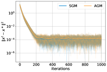
(a)

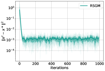
(b)

Figure 1: Strategic Prediction. (a) Iteration complexity of the norm-squared error to the Nash equilibrium for both the stochastic gradient method (SGM) and the adaptive gradient method (AGM) for a randomly generated problem instance where $m_{i}=10$ and $d_{i}=2$ for each $i\in\{1,2\}$. The sample complexity of AGM empirically matches that of SGM even for fairly large problem instances. (b) Iteration complexity of the norm-squared error to the performatively stable equilibrium for the stochastic repeated gradient method (SRGM) for a randomly generated problem instance where $m_{i}=100$ and $d_{i}=2$ for each $i\in\{1,2\}$. The empirical rates matches the theory in Section 4 and Section 6.

Recall in Section 5 in Example 2 we introduced a performative prediction game motivated by multiple election platforms. The decision problem that player $i$ faces is such that a set of features are drawn i.i.d. from a static distribution $\mathcal{P}_{\theta}$, and player $i$ observes a sample drawn from the conditional distribution

$$z_{i}|\theta\sim\varphi_{i}(\theta)+A_{i}x_{i}+A_{-i}x_{-i}+w_{i},$$

where $\varphi_{i}:\mathbb{R}^{d_{i}}\to\mathbb{R}$ is an arbitrary map, the parameter matrices $A_{i}\in\mathbb{R}^{m_{i}\times d_{i}}$ and $A_{-i}\in\mathbb{R}^{m_{i}\times d_{-i}}$ are fixed, and $w_{i}$ is a zero-mean random variable. Each player seeks to predict $z_{i}$ by minimizing the loss

$$\ell_{i}(x_{i},z_{i})=\frac{1}{2}\|z_{i}-\theta^{\top}x_{i}\|^{2}.$$

We showed in Example 2 that the map $x\mapsto H_{x}(y)$ is monotone as long as

$$\sqrt{n-1}\cdot\max_{i\in[n]}\|A_{-i}^{\top}A_{i}\|_{\rm op}\leq\min_{i\in[n]}\lambda_{\rm{min}}(A_{i}^{\top}A_{i}),.$$

As noted in Example 2, the interpretation is that the performative effects due to interaction with competitors are small relative to any player’s own performative effects. We enforce this condition on the parameters selected for the examples we explore numerically.

We randomly generate problem instances—namely, the parameters $A_{i},A_{-i}$ for $i\in[n]$—by using scipy.sparse.random which allows for the sparsity of the matrix to be set in addition to randomly generating the matrix parameters. We set $d=5$ and $m=100$ for the experiments in Figure 1. These values can be changed in the provided code, resulting in similar conclusions regarding the convergence rate. In Figure LABEL:fig:complexity_nash_synthetic we show the iteration complexity of the norm-square error to the Nash equilibrium for both the stochastic gradient method and the adaptive gradient method. Analogously, in Figure LABEL:fig:complexity_ps_synthetic, we show the iteration complexity of the norm-square error to the performatively stable equilibrium for the stochastic repeated gradient method. The mean and $\pm 1$ standard deviation are depicted with darker lines and the individual sample trajectories are shown using lighter shade lines of the same color indicated in the legend for the two methods. For both Nash-seeking methods (stochastic gradient and adaptive gradient method), we use a constant step size $\eta=0.01$ for both methods for the stochastic gradient update step. Additionally, we use the step size $\nu=2/(t+6d)$ for the estimation update in the adaptive gradient method. We see that their iteration complexities are empirically the same. For the performatively stable equilibrium seeking algorithm, we use a constant step-size $\eta=0.1$.

7.2 Revenue Maximization: Competition in Ride-Share Markets

The next numerical example we explore is semi-synthetic competition between two ride-share platforms seeking to maximize their revenue given that the demand they experience is influenced by their own prices as well as their competitors. We use data from a prior Kaggle competition to set up the semi-synthetic simulation environment.

Game Abstraction.

The abstraction for the game can be described as follows. Consider a ride-share market with two platforms that each seek to maximize their revenue by setting the price $x_{i}$. The vector of demands $z_{i}\in\mathbb{R}^{m_{i}}$ containing demand information for $m_{i}$ locations that each ride-share platform sees is influenced not only by the prices they set but also the prices that their competitor sets. Suppose that platform $i$’s loss is given by

$$\ell_{i}(x_{i},z_{i})=-\frac{1}{2}z_{i}^{\top}x_{i}+\frac{\lambda_{i}}{2}\|x_{i}\|^{2}$$

where $\lambda_{i}\geq 0$ is some regularization parameter, and $x_{i}\in\mathbb{R}^{m_{i}}$ represents the vector of price differentials from some nominal price for each of the $m_{i}$ locations. Observe that this game is separable since the losses $\ell_{i}$ do not explicitly depend on $x_{-i}$. Moreover, let us suppose that the random demand $z_{i}$ takes the semi-parametric form $z_{i}=\zeta_{i}+A_{i}x_{i}+A_{-i}x_{-i}$, where $\zeta_{i}$ follows some base distribution $\mathcal{P}_{i}$ and the parameters $A_{i}$ and $A_{-i}$ capture price elasticities to player $i$’s and its competitor’s change in price, respectively; naturally, the price elasticity for player $i$ to its own price changes is negative while the price elasticity for player $i$’s demand given changes in its competitors actions is positive. Namely, we have that $A_{i}\preceq 0$ and $A_{-i}\succeq 0$ capturing that an increase in player $i$’s prices results in a decrease in demand, while an increase in its competitor’s prices results in a increase in demand. Moreover, we showed in Example 1 that the mapping $x\mapsto H_{x}(y)$ is trivially monotone. Hence, the game between ride-share platforms is strongly monotone and admits a unique Nash equilibrium. Throughout the remainder of this section we set $\lambda_{1}=\lambda_{2}=1$.

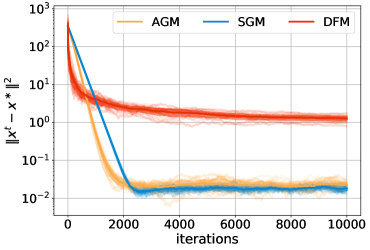
(a)

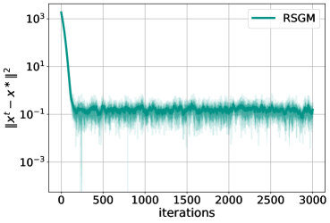
(b)

Figure 2: Competition in Ride-Share Markets: Experiment 1. (a) Iteration complexity for Nash seeking algorithms including derivative free gradient method (DFM), stochastic gradient method (SGM) and adaptive gradient method (AGM). (b) Iteration complexity for the repeated stochastic gradient method (RSGM), a performatively stable equilibrium seeking algorithm. The plots demonstrate that the sample complexities of AGM and SGM are nearly identical and outperform DFM as expected.

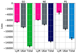
(a)

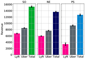
(b)

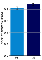
(c)

Figure 3: Competition in Ride-Share Markets: Experiment 2. (a) Loss and (b) revenue at the social optimum obtained via stochastic gradient descent on the social cost (sum of players’ costs), Nash equilibrium obtained via the stochastic gradient method, and performatively stable equilibrium obtained via the repeated stochastic gradient method. The overall (sum of both players) loss and revenue are worse at the performatively stable equilibrium. Note that the loss is the negative of the revenue plus some small $(\lambda_{1}=\lambda_{2}=1)$ regularization term. (c) Average price of anarchy (PoA) at the Nash equilibrum versus the performatively stable equilibrium. A value closer to one is better, and hence the Nash equilibrium (by a small margin) has a better PoA.

Semi-Synthetic Data Construction.

There are eleven locations that we consider in our simulation, and each element in $x_{i}$ represents the price difference (set by platform $i$) from a nominal price. We aggregate the rides into bins of $5 increments; this is done by taking the raw data and rounding the price to the nearest bin as follows $5\cdot\lfloor\frac{p}{5}\rfloor$ where $p$ is the price of the ride. Then, for each bin $j$ we have a different base empirical distribution $\mathcal{P}_{i,j}$ for each player $i\in\{1,2\}$ which is just the collection of rides for that bin.

For each bin, we estimate these price elasticity matrices $A_{i}$ and $A_{-i}$ from the data using the heuristic that a 50% increase in price by any firm leads to a 75% decrease in demand. With this heuristic we use the average base demand for each location and price bin pair to estimate both the diagonal elements of $A_{i}$ and $A_{-i}$. In the experiments presented, our semi-synthetic model is such that there is no correlation between locations; however, in the provided code base, we have additional experiments that estimate the correlation between locations and explore the effects of positive and negative correlations on equilibrium outcomes. We further note that the results presented in this section are for the $10 nominal price bin, however, in the repository of code it is easy to adjust this parameter to any of the other price bins. The conclusions we draw are similar across the bins.

Experiment 1: Numerical Comparison of Iteration Complexity.

To validate the theory developed in the previous sections, we show the iteration complexity of the Nash seeking algorithms (Figure LABEL:fig:complexity_nash), and the performatively stable equilibrium seeking algorithms (Figure LABEL:fig:complexity_ps). We run each algorithm from twenty random initial conditions, and compute the error between the trajectory of the algorithm and the Nash equilibrium (respectively, performatvely stable equilibrium). In Figure LABEL:fig:complexity_nash (respectively, Figure LABEL:fig:complexity_ps), we show the mean of these error trajectories and plus and minus one standard deviation. All the raw trajectories are also shown using a less opaque trajectory. For the stochastic gradient method, we use a constant step size $\eta=5e$-$5$ for the gradient update, and for the adaptive gradient method we use the step size schedule $\eta_{t}=\eta_{0}/t$ for the gradient update and $\nu_{t}=\nu_{0}/t$ for the estimation update where $\eta_{0}=5e$-$5$ and $\nu_{0}=1e$-$4$. For the derivative free method, we use a constant query radius $\delta=5$ and step size schedule $\eta_{t}=2/t$. The plots in Figure LABEL:fig:complexity_nash demonstrate the that empirical sample complexity of the adaptive gradient method and the stochastic gradient method are nearly identical, and outperform the derivative free method as expected. Figure LABEL:fig:complexity_ps simply illustrates the convergence rate as predicted by the theory in Section 4 for the repeated stochastic gradient method.

Experiment 2: Social Efficiency of Different Equilibrium Concepts.

As noted in the preceding sections, in the study of equilibrium for games, it is important to understand the efficiency of different equilibrium concepts. The typical benchmark for efficiency is the cost at the social optimum. The social cost is defined as the sum of all the players individual costs:

$$\mathcal{S}(x)=\sum_{i=1}^{n}\mathcal{L}_{i}(x).$$

We find the unique socially optimal equilibrium $x^{\tt so}$ by running stochastic gradient descent on the social cost (with $\eta=0.001$). Let $x^{\tt ne}$ be the Nash equilibrium of the game $(\mathcal{L}_{1},\mathcal{L}_{2})$ and let $x^{\tt ps}$ be the performatively stable equilibrium of the game $\mathcal{G}(x^{\tt ps})$, using the notation from Section 4 for the game induced by $x^{\tt ps}$.

To compute the Nash equilibrium and the perfomatively stable equilibrium we run the stochastic gradient method and the repeated stochastic gradient method with step-size $\eta=0.001$, respectively. In Figure 3 we show the loss at each of the equilibrium concepts for each player, and the total loss. For the ride-share game, both the Nash equilibrium and the performatively stable equilibrium are unique, and hence this set is a singleton.

The price anarchy is a common metric for equilibrium efficiency and is defined as the ratio of the social cost at the worst case competitive equilibrium concept relative to the social cost at the social optimum—namely, it is given by

$${\tt PoA}(x)=\frac{\max_{x\in{\tt Eq}(\mathcal{G})}\mathcal{S}(x)}{\mathcal{S}(x^{\tt so})},$$

where ${\tt Eq}(\mathcal{G})$ denotes the set of equilibria for the game $\mathcal{G}$. An equilibrium concept is said to be more efficient the closer this quantity is to one.

Given the stochastic nature of the problem at hand, we define the empirical price of anarchy as the ratio of the corresponding empirical social costs, and denote it as $\widehat{{\tt PoA}}(x)$. Hence, in comparing equilibrium concepts—i.e., Nash versus performatively stable equilibrium—the equilibrium with the social cost closest to the social cost at the social optimum is desirable. The empirical price of anarchy for the Nash equilibrium of the ride-share game is $\widehat{{\tt PoA}}(x^{\tt ne})=0.899$ while the empirical price of anarchy for the peformatively stable equilibrium is $\widehat{{\tt PoA}}(x^{\tt ps})=0.829$, where we compute the empirical social cost at the corresponding equilibrium. This is also illustrated in Figure LABEL:fig:poa. These ratios are fairly close, indicating that it is an interesting direction of future research to better understand the analytical properties of efficiency the different equilibrium concepts.

In Figure LABEL:fig:revenue, we also show the revenue for each of the equilibrium concepts. The revenue shares an analogous story to the loss: the total revenue at the Nash equilibrium is closer to the social optimum, but the performatively stable equilibrium is not far off.

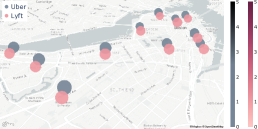
(a)

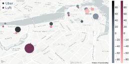
(b)

(c)

Figure 4: Competition in Ride-Share Markets: Experiment 2. Effects due to myopic decision-making. Change in (a) price, (b) demand and (c) revenue from nominal by location for $10 nominal price bin due to ignoring performative effects: players run stochastic gradient descent, and the image shows the change in demand (respectively, revenue) when both players model decision-dependence as compared to when they both do not model decision-dependence. The size of the circles shows the magnitude of the change, while the color indicates the raw value. The majority of locations see a decrease in demand, but due to an increase in price at the Nash equilibrium relative to the myopic outcome, there is an increase in revenue for both players.

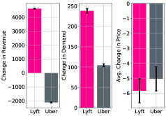
(a)

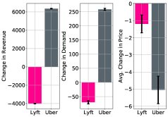
(b)

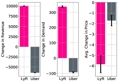
(c)

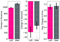
(d)

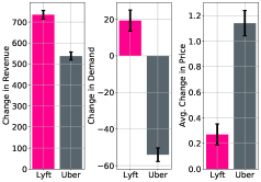
(e)

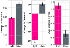
(f)

Figure 5: Competition in Ride-Share Markets: Experiment 3. Effects of players being (a)–(c) myopic or (d)–(f) partially myopic relative to Nash (not myopic, and consider competition). Positive changes in revenue indicate the Nash equilibrium is better for that player. When a player is myopic, they do not consider any performative effects in their update—i.e., $g_{i}^{t}=\lambda_{i}x_{i}^{t}-\frac{1}{2}\zeta_{i}^{t}$—and when a player is partially myopic, they consider their own performative effects, but not those of their competitor—i.e., $g_{i}^{t}=-(A_{i}-\lambda_{i}I)^{\top}x_{i}^{t}-\frac{1}{2}\zeta_{i}^{t}$. In (a)–(c), we observe that when at least one player is completely myopic, then at least one player is worse off at the Nash equilibrium. In (d)–(f) we observe that when at least one player is partially myopic, the Nash equilibrium always is better for both players.

Experiment 3: Effect of Ignoring Performativity.

We study the impact of players ignoring performative effects due to competition in the data distribution. In Figure 5, we explore the effects of players either being completely myopic—i.e., $g_{i}^{t}=\lambda_{i}x_{i}^{t}-\frac{1}{2}\zeta_{i}^{t}$—or partially myopic—i.e., $g_{i}^{t}=-(A_{i}-\lambda_{i}I)^{\top}x_{i}^{t}-\frac{1}{2}\zeta_{i}^{t}$—on the change in revenue, demand and average price (across locations) from nominal at the Nash equilibrium. Recall that players employing the stochastic gradient method use the gradient estimate $g_{i}^{t}=-(A_{i}-\lambda_{i}I)^{\top}x_{i}^{t}-\frac{1}{2}(\zeta_{i}^{t}+A_{-i}x_{-i}^{t})$; we refer to this as the non-myopic case since all performative effects are considered. Even when the players are myopic or partially myopic, the environment, however, does have these performative effects, meaning that $z_{i}=\zeta_{i}+A_{i}x_{i}+A_{-i}x_{-i}$ and hence, the myopic player is in this sense ignoring or unaware of the fact that the data distribution is reacting to its competition’s decisions. To compute the equilibrium outcomes we run the stochastic gradient method with a constant step-size of $\eta=0.001$.

In Figure 5 (a)–(c), we observe that when at least one player is completely myopic, then at least one player is worse off at the Nash equilibrium in the sense that their revenue is lower. Interestingly, the player that is worse off at the Nash is the non-myopic player. In Figure 5 (d)–(f), on the other hand, we observe that when at least one player is partially myopic, the Nash equilibrium always is better for both players in the sense that their individual revenues are higher at the Nash.

The values in Figure 5 represent the total demand and revenue changes, and average price change across locations. It is also informative to examine the per-location changes. Focusing in on the setting considered in Figure 5 (d), we examine the per-location price, revenue and demand. We see that the relative change depends on the location, however, the majority of locations see a decrease in demand, yet an increase in price and hence, revenue. This suggests that modeling performative effects due to competition can be beneficial for both players.

8 Discussion

The new class of games in this paper motivates interesting future work at the intersection of statistical learning theory and game theory. For instance, it is of interest to extend the present framework to handle more general parametric forms of the distributions $\mathcal{D}_{i}$. Many multiplayer performative prediction problems exhibit a hierarchical structure such as a governing body that presides over an institution; hence, a Stackelberg variant of multiplayer performative prediction is of interest. Along these lines, the multiplayer performative prediction problem is also of interest for mechanism design problems arising in applications such as recommender systems. For instance, the recommendations that platforms select at the Nash equilibrium influence the preferences of consumers (data-generators). A mechanism designer (e.g., the government) can place constraints on platforms to prevent them from manipulating users’ preferences to make their prediction tasks easier.

  

Appendix

Appendix A Stochastic gradient method with bias

In this section, we consider a variational inequality

$$0\in G(x)+N_{\mathcal{X}}(x),$$ (30)

where $\mathcal{X}\subset\mathbb{R}^{d}$ is a closed convex set and $G\colon\mathbb{R}^{d}\to\mathbb{R}^{d}$ is an $L$-Lipschitz continuous and $\alpha$-strongly monotone map. We will analyze the stochastic gradient method, which in each iteration performs the update:

$$x^{t+1}=\operatorname{proj}_{\mathcal{X}}(x^{t}-\eta g^{t}),$$ (31)

where $\eta>0$ is a fixed stepsize and $g_{t}$ is a sequence of random variables, which approximates $G(x^{t})$. In particular, it will be crucial for us to allow $g^{t}$ to be a biased estimator of $G(x^{t})$. Formally, we make the following assumption on the randomness in the process. Throughout, $x^{\star}$ denotes the unique solution of (30).

Assumption 12 (Stochastic framework).

Suppose that there exists a filtered probability space $(\Omega,\mathcal{F},\mathbb{F},\mathbb{P})$ with filtration $\mathbb{F}=(\mathcal{F}_{t})_{t\geq 0}$ such that $\mathcal{F}_{0}=\{\emptyset,\Omega\}$. Suppose moreover that $g_{t}$ is $\mathcal{F}_{t+1}$-measurable and there exist constants $B,\sigma\geq 0$ and $\mathcal{F}_{t}$-measurable random variables $C_{t},\sigma_{t}\geq 0$ satisfying the bias/variance bounds

$${\rm\bf(Bias)}\qquad\qquad\|\mathbb{E}_{t}g^{t}-G(x^{t})]\| \leq C_{t}+B\|x^{t}-x^{*}\|,$$

$${\rm\bf(Variance)}\qquad\qquad\mathbb{E}_{t}\|g^{t}-\mathbb{E}_{t}[g^{t}]\|^{2} \leq\sigma^{2}_{t}+D^{2}\|x^{t}-x^{\star}\|^{2},$$

where $\mathbb{E}_{t}=\operatorname*{\mathbb{E}}[\cdot\mid\mathcal{F}_{t}]$ denotes the conditional expectation.

The following is a one-step improvement guarantee for the stochastic gradient method in the two conceptually distinct cases $C_{t}=0$ and $B=0$. In the case $C_{t}=0$ , the bias $\mathbb{E}_{t}g^{t}-G(x^{t})$ shrinks as the iterates approach $x^{\star}$. The theorem shows that as long as $B/\alpha<1$, with a sufficiently small stepsize $\eta$, the method can converge to an arbitrarily small neighborhood of $x^{\star}$. In the case $B=0$, one can only hope to convergence to a neighborhood of the minimizer whose radius depends on $\{C_{t}\}_{t\geq 0}$.

Theorem 8 (One step improvement).

The following are true.

• (Benign bias) Suppose $C_{t}\equiv 0$ for all $t$. Set $\rho:=B/\alpha$ and suppose that we are in the regime $\rho\in(0,1)$. Then with any $\eta<\frac{\alpha(1-\rho)}{8L^{2}}$, the stochastic gradient method (31) generates a sequence $x^{t}$ satisfying

  $$\mathbb{E}_{t}\|x^{t+1}-x^{\star}\|^{2}\leq\frac{1+2\eta\alpha\rho+4\eta^{2}D^{2}+2\eta^{2}\alpha^{2}\rho^{2}}{1+2\eta\alpha(\frac{1+\rho}{2})}\|x^{t}-x^{\star}\|^{2}+\frac{4\eta^{2}\sigma^{2}_{t}}{1+2\eta\alpha(\frac{1+\rho}{2})}.$$ (32)

• (Offset bias) Suppose $B\equiv 0$. Then with any $\eta\leq\frac{\alpha}{4L^{2}}$, the stochastic gradient method (31) generates a sequence $x^{t}$ satisfying

  $$\mathbb{E}_{t}\|x^{t+1}-x^{\star}\|^{2}\leq\frac{1+2\eta^{2}D^{2}}{1+\eta\alpha}\|x^{t}-x^{\star}\|^{2}+\frac{2\eta^{2}\sigma^{2}_{t}}{1+\eta\alpha}+\frac{2\eta C_{t}^{2}}{\alpha(1+\eta\alpha)}.$$ (33)

  Moreover, in the zero bias setting $B\equiv C_{t}\equiv 0$, the estimate (33) holds in the slightly wider parameter regime $\eta\leq\frac{\alpha}{2L^{2}}$.

Proof.

We begin with the first claim. To this end, suppose $C_{t}\equiv 0$ for all $t$. Set $\rho:=B/\alpha$ and suppose that we are in the regime $\rho\in(0,1)$. Fix three constants $\Delta_{1},\Delta_{2},\Delta_{3}>0$ to be specified later. Noting that $x^{t+1}$ is the minimizer of the $1$-strongly convex function $x\mapsto\frac{1}{2}\|x^{t}-\eta g^{t}-x\|^{2}$ over $\mathcal{X}$, we deduce

$$\frac{1}{2}\|x^{t+1}-x^{\star}\|^{2}\leq\frac{1}{2}\|x^{t}-\eta g^{t}-x^{\star}\|^{2}-\frac{1}{2}\|x^{t}-\eta g^{t}-x^{t+1}\|^{2}.$$

Expanding the squares on the right hand side and combining terms yields

$$\frac{1}{2}\|x^{t+1}-x^{\star}\|^{2} \leq\frac{1}{2}\|x^{t}-x^{\star}\|^{2}-\eta\langle g^{t},x^{t+1}-x^{\star}\rangle-\frac{1}{2}\|x^{t+1}-x^{t}\|^{2}$$

$$=\frac{1}{2}\|x^{t}-x^{\star}\|^{2}-\eta\langle g^{t},x^{t}-x^{\star}\rangle-\frac{1}{2}\|x^{t+1}-x^{t}\|^{2}-\eta\langle g^{t},x^{t+1}-x^{t}\rangle.$$

Setting $\mu^{t}:=\operatorname*{\mathbb{E}}_{t}[g^{t}]$, we successively compute

$$\frac{1}{2}\mathbb{E}_{t}\|x^{t+1}-x^{\star}\|^{2} \leq\frac{1}{2}\|x^{t}-x^{\star}\|^{2}-\eta\langle\mathbb{E}_{t}g^{t},x^{t}-x^{\star}\rangle-\frac{1}{2}\mathbb{E}_{t}\|x^{t+1}-x^{t}\|^{2}-\eta\mathbb{E}_{t}\langle g^{t},x^{t+1}-x^{t}\rangle$$

$$\leq\frac{1}{2}\|x^{t}-x^{\star}\|^{2}-\eta\langle\mu^{t},x^{t}-x^{\star}\rangle-\frac{1}{2}\mathbb{E}_{t}\|x^{t+1}-x^{t}\|^{2}-\eta\mathbb{E}_{t}\langle g^{t},x^{t+1}-x^{t}\rangle$$

$$=\frac{1}{2}\|x^{t}-x^{\star}\|^{2}-\eta\mathbb{E}_{t}\langle G(x^{t+1}),x^{t+1}-x^{\star}\rangle-\frac{1}{2}\mathbb{E}_{t}\|x^{t+1}-x^{t}\|^{2}$$

$$+\eta\underbrace{\mathbb{E}_{t}\langle g^{t}-\mu^{t},x^{t}-x^{t+1}\rangle}_{P_{1}}+\eta\underbrace{\mathbb{E}_{t}\langle\mu^{t}-G(x^{t+1}),x^{\star}-x^{t+1}\rangle}_{P_{2}}].$$ (34)

Taking into account strong monotonicity of $G$, we deduce $\langle G(x^{t+1}),x^{t+1}-x^{\star}\rangle\geq\alpha\|x^{t+1}-x^{\star}\|^{2}$ and therefore

$$\frac{1+2\eta\alpha}{2}\mathbb{E}_{t}\|x^{t+1}-x^{\star}\|^{2}\leq\frac{1}{2}\|x^{t}-x^{\star}\|^{2}-\frac{1}{2}\mathbb{E}_{t}\|x^{t+1}-x^{t}\|^{2}+\eta(P_{1}+P_{2}).$$ (35)

Using Young’s inequality, we may upper bound $P_{1}$ and $P_{2}$ by:

$$P_{1}\leq\frac{\sigma^{2}_{t}+D^{2}\|x^{t}-x^{\star}\|^{2}}{2\Delta_{1}}+\frac{\Delta_{1}\mathbb{E}_{t}\|x^{t+1}-x^{t}\|^{2}}{2}.$$ (36)

Next, we decompose $P_{2}$ as

$$P_{2}=\langle\mu^{t}-G(x^{t}),x^{\star}-x^{t}\rangle+\mathbb{E}_{t}\langle\mu^{t}-G(x^{t}),x^{t}-x^{t+1}\rangle+\mathbb{E}_{t}\langle G(x^{t})-G(x^{t+1}),x^{\star}-x^{t+1}\rangle.$$ (37)

We bound each of the three products in turn. The first bound follows from our assumption on the bias:

$$\langle\mu^{t}-G(x^{t}),x^{\star}-x^{t}\rangle\leq B\|x^{t}-x^{\star}\|^{2}.$$ (38)

The second bound uses Young’s inequality and our assumption on the bias:

$$\mathbb{E}_{t}\langle\mu^{t}-G(x^{t}),x^{t}-x^{t+1}\rangle \leq\frac{\Delta_{2}\|\mu^{t}-G(x^{t})\|^{2}}{2}+\frac{\mathbb{E}_{t}\|x^{t}-x^{t+1}\|^{2}}{2\Delta_{2}}$$ (39)

$$\leq\frac{\Delta_{2}B^{2}\|x^{t}-x^{\star}\|^{2}}{2}+\frac{\mathbb{E}_{t}\|x^{t}-x^{t+1}\|^{2}}{2\Delta_{2}}$$

The third inequality uses Young’s inequality and Lipschitz continuity of $G$:

$$\mathbb{E}_{t}\langle G(x^{t})-G(x^{t+1}),x^{\star}-x^{t+1}\rangle \leq\frac{\Delta_{3}\|G(x^{t})-G(x^{t+1})\|^{2}}{2}+\frac{\mathbb{E}_{t}\|x^{\star}-x^{t+1}\|^{2}}{2\Delta_{3}}$$ (40)

$$\leq\frac{\Delta_{3}L^{2}\|x^{t}-x^{t+1}\|^{2}}{2}+\frac{\mathbb{E}_{t}\|x^{\star}-x^{t+1}\|^{2}}{2\Delta_{3}}$$

Putting together all the estimates (35)-(40) yields

$$\frac{1+2\eta\alpha-2\eta\Delta_{3}^{-1}}{2}\mathbb{E}_{t}\|x^{t+1}-x^{\star}\|^{2} \leq\frac{1+\eta D^{2}\Delta^{-1}_{1}+2\eta B+\eta\Delta_{2}B^{2}}{2}\|x^{t}-x^{\star}\|^{2}$$ (41)

$$~{}~{}~{}-\frac{1-\eta\Delta_{1}-\eta\Delta_{2}^{-1}-\eta\Delta_{3}L^{2}}{2}\mathbb{E}_{t}\|x^{t+1}-x^{t}\|^{2}+\frac{\eta\sigma^{2}_{t}}{2\Delta_{1}}.$$

Let us now set

$$\Delta_{3}^{-1}=\frac{(1-\rho)\alpha}{2},\qquad\Delta_{1}=\frac{1}{4\eta},\qquad\Delta_{2}^{-1}:=\eta^{-1}-\Delta_{1}-\Delta_{3}L^{2}.$$

Notice $\Delta_{1}\leq\frac{1}{2\eta}-\Delta_{3}L^{2}$ by our assumption that $\eta\leq\frac{\alpha(1-\rho)}{8L^{2}}$. In particular, this implies $\Delta_{2}^{-1}\geq\frac{1}{2\eta}$. Notice that our choice of $\Delta_{2}$ ensures that the the fraction multiplying $\mathbb{E}_{t}\|x^{t+1}-x^{t}\|^{2}$ in (41) is zero. We therefore deduce

$$\mathbb{E}_{t}\|x^{t+1}-x^{\star}\|^{2} \leq\frac{1+\eta D^{2}\Delta^{-1}_{1}+2\eta B+\eta\Delta_{2}B^{2}}{1+2\eta\alpha-2\eta\Delta_{3}^{-1}}\|x^{t}-x^{\star}\|^{2}+\frac{\eta\sigma^{2}_{t}}{\Delta_{1}(1+2\eta\alpha-2\eta\Delta_{3}^{-1})}$$

$$\leq\frac{1+2\eta\alpha\rho+4\eta^{2}D^{2}+2\eta^{2}\alpha^{2}\rho^{2}}{1+2\eta\alpha(\frac{1+\rho}{2})}\|x^{t}-x^{\star}\|^{2}+\frac{4\eta^{2}\sigma^{2}_{t}}{1+2\eta\alpha(\frac{1+\rho}{2})},$$

thereby completing the proof of (32).

We next prove the second claim. To this end, suppose $B=0$. All of the reasoning leading up to and including (36) is valid. Continuing from this point, using Young’s inequality, we upper bound $P_{2}$ by:

$$P_{2}\leq\frac{\mathbb{E}_{t}\|\mu^{t}-G(x^{t+1})\|^{2}}{2\Delta_{2}}+\frac{\Delta_{2}\mathbb{E}_{t}\|x^{t+1}-x^{\star}\|^{2}}{2}.$$ (42)

Next observe

$$\mathbb{E}_{t}\|\mu^{t}-G(x^{t+1})\|^{2} \leq 2\mathbb{E}_{t}\|\mu^{t}-G(x^{t})\|^{2}+2\mathbb{E}_{t}\|G(x^{t})-G(x^{t+1})\|^{2},$$ (43)

$$\leq 2C_{t}^{2}+2L^{2}\|x^{t}-x^{t+1}\|^{2}$$

and therefore

$$P_{2}\leq\frac{2C_{t}^{2}+2L^{2}\|x^{t}-x^{t+1}\|^{2}}{2\Delta_{2}}+\frac{\Delta_{2}\mathbb{E}_{t}\|x^{t+1}-x^{\star}\|^{2}}{2}$$ (44)

Putting the estimates (35), (36), and (44) together yields:

$$\frac{1+\eta(2\alpha-\Delta_{2})}{2}\mathbb{E}_{t}\|x^{t+1}-x^{\star}\|^{2} \leq\frac{1+\eta D^{2}\Delta_{1}^{-1}}{2}\|x^{t}-x^{\star}\|^{2}$$ (45)

$$+\frac{\eta\sigma^{2}_{t}}{2\Delta_{1}}+\frac{2\eta C_{t}^{2}\Delta_{2}^{-1}}{2}-\frac{1-2\eta L^{2}\Delta_{2}^{-1}-\eta\Delta_{1}}{2}\mathbb{E}_{t}\|x^{t+1}-x^{t}\|^{2}$$

Setting $\Delta_{2}=\alpha$ and $\Delta_{1}=\eta^{-1}-\frac{2L^{2}}{\alpha}$ ensures that the last term on the right is zero. Notice that our assumption $\eta\leq\frac{\alpha}{4L^{2}}$ ensures $\Delta_{1}\geq\frac{1}{2\eta}$. Rearranging (45) directly yields (33). In the case $B\equiv C_{t}\equiv 0$, instead of (43) we may simply use the bound $\mathbb{E}_{t}\|\mu^{t}-G(x^{t+1})\|^{2}=\mathbb{E}_{t}\|G(x^{t})-G(x^{t+1})\|\leq L^{2}\|x^{t}-x^{t+1}\|^{2}$. Continuing in the same way as above yields the improved estimate. ∎

Appendix B Technical results on sequences

The following lemma is standard and follows from a simple inductive argument.

Lemma 8.

Consider a sequence $D_{t}\geq 0$ for $t\geq 1$ and constants $t_{0}\geq 0$, $a>0$ satisfying

$$D_{t+1}\leq(1-\tfrac{2}{t+t_{0}})D_{t}+\tfrac{a}{(t+t_{0})^{2}}$$ (46)

Then the estimate holds:

$$D_{t}\leq\frac{\max\{(1+t_{0})D_{1},a\}}{t+t_{0}}\qquad\forall t\geq 1.$$ (47)

We will need the following more general version of the lemma.

Lemma 9.

Consider a sequence $D_{t}\geq 0$ for $t\geq 1$ and constants $t_{0}\geq 0$, $a,b>0$ satisfying

$$D_{t+1}\leq(1-\tfrac{2}{t+t_{0}})D_{t}+\tfrac{a}{(t+t_{0})^{2}}+\tfrac{b}{(t+t_{0})^{3}}.$$ (48)

Then the estimate holds:

$$D_{t}\leq\frac{\max\{(1+t_{0})D_{1}/2,a\}}{t+t_{0}}+\frac{\max\{(1+t_{0})^{3/2}D_{1}/2,b\}}{(t+t_{0})^{3/2}}\qquad\forall t\geq 1.$$ (49)

Proof.

Clearly the recursion (48) continues to hold with $a$ and $b$ replaced by the bigger quantities $\max\{(1+t_{0})D_{1}/2,a\}$ and $\max\{(1+t_{0})D_{1}/2,b\}$, respectively. Therefore abusing notation, we will make this substitution. As a consequence, the claimed estimate (49) holds automatically for the base case $t=1$. As an inductive assumption, suppose the claim (49) is true for $D_{t}$. Set $s=t+t_{0}$. We then deduce

$$D_{t+1} \leq\left(1-\frac{2}{s}\right)D_{t}+\frac{a}{s^{2}}+\frac{b}{s^{3}}$$

$$\leq\left(1-\frac{2}{s}\right)\left(\frac{a}{s}+\frac{b}{s^{3/2}}\right)+\frac{a}{s^{2}}+\frac{b}{s^{3}}$$

$$\leq a\left(\frac{1}{s}-\frac{1}{s^{2}}\right)+b\left(\frac{1}{s^{3/2}}-\frac{2}{s^{5/2}}+\frac{1}{s^{3}}\right).$$

Elementary algebraic manipulations show $\frac{1}{s}-\frac{1}{s^{2}}\leq\frac{1}{s+1}$. Define the function $\phi(s)=\frac{1}{s^{3/2}}-\frac{2}{s^{5/2}}+\frac{1}{s^{3}}-\frac{1}{(1+s)^{3/2}}$. Elementary calculus shows that $\phi$ is increasing on the interval $s\in[1,\infty)$. Since $\phi$ tends to zero as $s$ tends to infinity, it follows that $\phi$ is negative on the interval $[1,\infty)$. We therefore conclude $D_{t+1}\leq\frac{a}{s+1}+\frac{b}{(1+s)^{3/2}}$ as claimed. ∎

Appendix C Online Least Squares

In this appendix section, we record basic and well-known results on estimation in online least squares, following [Dieuleveut et al., 2017].

Lemma 10.

Fix a probability space $(\Omega,\mathcal{F},\mathbb{P})$ with two sub-$\sigma$-algebras $\mathcal{G}_{1}\subset\mathcal{G}_{2}\subset\mathcal{F}$ . Define the function

$$f(B)=\frac{1}{2}\|By-b\|^{2},$$

where $B\colon\Omega\to\mathbb{R}^{m_{1}\times m_{2}}$, $b\colon\Omega\to\mathbb{R}^{m_{1}}$, and $y\colon\Omega\to\mathbb{R}^{m_{2}}$ are random variables. Suppose moreover that there exist random variables $V\colon\Omega\to\mathbb{R}^{m_{1}\times m_{2}}$ and $\sigma\colon\Omega\to\mathbb{R}$ satisfying the following.

1. $B$, $V$, and $\sigma_{1}$ are $\mathcal{G}_{1}$-measurable.

2. $y$ is $\mathcal{G}_{2}$-measurable.

3. The estimates, $\operatorname*{\mathbb{E}}[b\mid\mathcal{G}_{2}]=Vy$ and $\operatorname*{\mathbb{E}}[\|Vy-b\|^{2}\mid\mathcal{G}_{2}]\leq\sigma^{2}$ ,hold.

4. There exist constants $\lambda_{1},\lambda_{2},R>0$ satisfying

   $$\lambda_{1}I\preceq\mathbb{E}[yy^{\top}\mid\mathcal{G}_{1}],\qquad\mathbb{E}[\|y\|^{2}\mid\mathcal{G}_{1}]\leq\lambda_{2},\qquad\textrm{and}\qquad\operatorname*{\mathbb{E}}[\|y\|^{2}yy^{\top}\mid\mathcal{G}_{1}]\preceq R^{2}\operatorname*{\mathbb{E}}[yy^{\top}].$$

Then for any constant $\nu\in(0,\frac{2}{R^{2}})$, the gradient step $B^{+}=B-\nu(By-b)y^{\top}$ satisfies the bound:

$$\frac{1}{2}\mathbb{E}[\|B^{+}-V\|^{2}_{F}\mid\mathcal{G}_{1}]\leq\frac{1-\lambda_{1}\nu(2-\nu R^{2})}{2}\|B-V\|^{2}_{F}+\frac{\nu^{2}\sigma^{2}\lambda_{2}}{2}.$$

Proof.

Expanding the squared norm yields:

$$\frac{1}{2}\|B^{+}-V\|^{2}_{F}=\frac{1}{2}\|B-V-\nu(By-b)y^{\top}\|^{2}_{F} =\frac{1}{2}\|B-V\|^{2}_{F}-\nu\langle B-V,(By-b)y^{\top}\rangle$$

$$\quad+\frac{\nu^{2}}{2}\|(By-b)y^{\top}\|^{2}_{F}.$$

Taking conditional expectations, we conclude

$$\frac{1}{2}\mathbb{E}[\|B^{+}-V\|^{2}_{F}\mid\mathcal{G}_{2}] =\frac{1}{2}\|B-V\|^{2}_{F}-\nu\langle B-V,(By-\mathbb{E}[b\mid\mathcal{G}_{2}])y^{\top}\rangle+\frac{\nu^{2}}{2}\mathbb{E}[\|(By-b)y^{\top}\|^{2}_{F}\mid\mathcal{G}_{2}]$$ (50)

$$=\frac{1}{2}\|B-V\|^{2}_{F}-\nu\|(B-V)y\|_{F}^{2}+\frac{\nu^{2}}{2}\|y\|^{2}\mathbb{E}[\|By-b\|^{2}_{F}\mid\mathcal{G}_{2}].$$

Next, observe

$$\|By-b\|^{2}_{F}=\|(B-V)y\|^{2}+\|Vy-b\|^{2}+2\langle By-Vy,Vy-b\rangle.$$

Taking the conditional expectation $\mathbb{E}[\cdot\mid\mathcal{G}_{2}]$, the last term vanishes, and therefore we deduce $\mathbb{E}[\|By-b\|^{2}_{F}\mid\mathcal{F}^{\prime}]\leq\|(B-V)y\|^{2}+\sigma^{2}$. Combining this with (50) we compute

$$\frac{1}{2}\mathbb{E}[\|B^{+}-V\|^{2}_{F}\mid\mathcal{G}_{2}] \leq\frac{1}{2}\|B-V\|^{2}_{F}-\nu\|(B-V)y\|_{F}^{2}+\frac{\nu^{2}}{2}\|y\|^{2}\|(B-V)y\|^{2}+\frac{\nu^{2}\sigma^{2}}{2}\|y\|^{2}.$$

Taking expectations with respect to $\mathcal{G}_{1}$ and using the tower rule, we deduce

$$\frac{1}{2}\mathbb{E}[\|B^{+}-V\|^{2}_{F}\mid\mathcal{G}_{1}] \leq\frac{1}{2}\|B-V\|^{2}_{F}-\nu\operatorname*{\mathbb{E}}[\|(B-V)y\|_{F}^{2}\mid\mathcal{G}_{1}]+\frac{\nu^{2}}{2}\operatorname*{\mathbb{E}}[\|y\|^{2}\|(B-V)y\|^{2}\mid\mathcal{G}_{1}]$$

$$\quad+\frac{\nu^{2}\sigma^{2}\lambda_{2}}{2}.$$

Observe next

$$\operatorname*{\mathbb{E}}[\|y\|^{2}\|(B-V)y\|^{2}\mid\mathcal{G}_{1}]=\langle(B-V)(B-V)^{\top},\mathbb{E}[\|y\|^{2}yy^{\top}\mid\mathcal{G}_{1}]]\rangle\leq R^{2}\mathbb{E}[\|(B-V)y\|_{F}^{2}\mid\mathcal{G}_{1}],$$

and therefore

$$\frac{1}{2}\mathbb{E}[\|B^{+}-V\|^{2}_{F}\mid\mathcal{G}_{1}] \leq\frac{1}{2}\|B-V\|^{2}_{F}-(\nu-\frac{\nu^{2}R^{2}}{2})\operatorname*{\mathbb{E}}[\|(B-V)y\|_{F}^{2}\mid\mathcal{G}_{1}]+\frac{\nu^{2}\sigma^{2}\lambda_{2}}{2}$$

Note that $\nu\geq\frac{\nu^{2}R^{2}}{2}$. Next we estimate

$$\operatorname*{\mathbb{E}}[\|(B-V)y\|_{F}^{2}\mid\mathcal{G}_{1}] =\textrm{tr}((B-V)^{\top}(B-V)\operatorname*{\mathbb{E}}[yy^{\top}\mid\mathcal{G}_{1}]]\rangle\geq\lambda_{1}\|B-V\|^{2}_{F}.$$

This completes the proof. ∎

References

• Ahmed [2000] Shabbir Ahmed. Strategic planning under uncertainty: Stochastic integer programming approaches. University of Illinois at Urbana-Champaign, 2000.
• Angwin et al. [2016] Julia Angwin, Jeff Larson, Surya Mattu, and Lauren Kirchner. Machine bias. Propublica, 2016. URL https://www.propublica.org/article/machine-bias-risk-assessments-in-criminal-sentencing.
• Bartlett et al. [2019] Robert Bartlett, Adair Morse, Richard Stanton, and Nancy Wallace. Consumer-lending discrimination in the fintech era. Technical report, National Bureau of Economic Research, 2019.
• Bechavod et al. [2020] Yahav Bechavod, Katrina Ligett, Zhiwei Steven Wu, and Juba Ziani. Causal feature discovery through strategic modification. arXiv preprint arXiv:2002.07024, 3, 2020.
• Bravo et al. [2018] Mario Bravo, David S Leslie, and Panayotis Mertikopoulos. Bandit learning in concave $n$-person games. arXiv preprint arXiv:1810.01925, 2018.
• Brown et al. [2020] Gavin Brown, Shlomi Hod, and Iden Kalemaj. Performative prediction in a stateful world. arXiv preprint arXiv:2011.03885, 2020.
• Chasnov et al. [2020] Benjamin Chasnov, Lillian Ratliff, Eric Mazumdar, and Samuel Burden. Convergence analysis of gradient-based learning in continuous games. In Ryan P. Adams and Vibhav Gogate, editors, Proceedings of The 35th Uncertainty in Artificial Intelligence Conference, volume 115 of Proceedings of Machine Learning Research, pages 935–944. PMLR, 22–25 Jul 2020.
• Chen et al. [2015] Le Chen, Alan Mislove, and Christo Wilson. Peeking beneath the hood of uber. In Proceedings of the 2015 Internet Measurement Conference, IMC ’15, page 495–508, 2015. doi: 10.1145/2815675.2815681.
• Courtland [2018] R Courtland. Bias detectives: the researchers striving to make algorithms fair. Nature, pages 357–360, 2018. doi: 10.1038/d41586-018-05469-3.
• Cutler et al. [2021] Joshua Cutler, Dmitriy Drusvyatskiy, and Zaid Harchaoui. Stochastic optimization under time drift: iterate averaging, step decay, and high probability guarantees. arXiv preprint arXiv:2108.07356, 2021.
• Diethe et al. [2019] Tom Diethe, Tom Borchert, Eno Thereska, Borja Balle, and Neil Lawrence. Continual learning in practice. arXiv preprint arXiv:1903.05202, 2019.
• Dieuleveut et al. [2017] Aymeric Dieuleveut, Nicolas Flammarion, and Francis Bach. Harder, better, faster, stronger convergence rates for least-squares regression. The Journal of Machine Learning Research, 18(1):3520–3570, 2017.
• Dong et al. [2018] Jinshuo Dong, Aaron Roth, Zachary Schutzman, Bo Waggoner, and Zhiwei Steven Wu. Strategic classification from revealed preferences. In Proceedings of the 2018 ACM Conference on Economics and Computation, pages 55–70, 2018.
• Drusvyatskiy and Xiao [2020] Dmitriy Drusvyatskiy and Lin Xiao. Stochastic optimization with decision-dependent distributions. arXiv preprint arXiv:2011.11173, 2020.
• Drusvyatskiy et al. [2021] Dmitriy Drusvyatskiy, Maryam Fazel, and Lillian J. Ratliff. Improved rates for derivative free gradient play in monotone games. arXiv:2111.09456, 2021.
• Dupacová [2006] Jitka Dupacová. Optimization under exogenous and endogenous uncertainty. University of West Bohemia in Pilsen, 2006.
• Ermoliev [1988] Yu. Ermoliev. Stochastic quasigradient methods. In Yu. Ermoliev and R. J-B Wets, editors, Numerical Techniques for Stochastic Optimization, chapter 6, pages 141–185. Springer, 1988.
• Gaivoronskii [1978] A. A. Gaivoronskii. Nonstationary stochastic programming problems. Cybernetics, 14:575–579, 1978.
• Ghadimi and Lan [2013] Saeed Ghadimi and Guanghui Lan. Optimal stochastic approximation algorithms for strongly convex stochastic composite optimization, ii: shrinking procedures and optimal algorithms. SIAM Journal on Optimization, 23(4):2061–2089, 2013.
• Hardt et al. [2016] Moritz Hardt, Nimrod Megiddo, Christos Papadimitriou, and Mary Wootters. Strategic classification. In Proceedings of the 2016 ACM conference on innovations in theoretical computer science, pages 111–122, 2016.
• Hellemo et al. [2018] Lars Hellemo, Paul I Barton, and Asgeir Tomasgard. Decision-dependent probabilities in stochastic programs with recourse. Computational Management Science, 15(3):369–395, 2018.
• Izzo et al. [2021] Zachary Izzo, Lexing Ying, and James Zou. How to learn when data reacts to your model: performative gradient descent. arXiv preprint arXiv:2102.07698, 2021.
• Jonsbråten et al. [1998] Tore W Jonsbråten, Roger JB Wets, and David L Woodruff. A class of stochastic programs withdecision dependent random elements. Annals of Operations Research, 82:83–106, 1998.
• Lum and Isaac [2016] Kristian Lum and William Isaac. To predict and serve? Significance, 13(5):14–19, 2016.
• Mendler-Dünner et al. [2020] Celestine Mendler-Dünner, Juan Perdomo, Tijana Zrnic, and Moritz Hardt. Stochastic optimization for performative prediction. In H. Larochelle, M. Ranzato, R. Hadsell, M. F. Balcan, and H. Lin, editors, Advances in Neural Information Processing Systems, volume 33, pages 4929–4939. Curran Associates, Inc., 2020.
• Mertikopoulos and Zhou [2019] Panayotis Mertikopoulos and Zhengyuan Zhou. Learning in games with continuous action sets and unknown payoff functions. Mathematical Programming, 173(1):465–507, 2019.
• Miller et al. [2020] John Miller, Smitha Milli, and Moritz Hardt. Strategic classification is causal modeling in disguise. In International Conference on Machine Learning, pages 6917–6926. PMLR, 2020.
• Miller et al. [2021] John Miller, Juan C Perdomo, and Tijana Zrnic. Outside the echo chamber: Optimizing the performative risk. arXiv preprint arXiv:2102.08570, 2021.
• Perdomo et al. [2020] Juan Perdomo, Tijana Zrnic, Celestine Mendler-Dünner, and Moritz Hardt. Performative prediction. In International Conference on Machine Learning, pages 7599–7609. PMLR, 2020.
• Ratliff et al. [2016] Lillian J Ratliff, Samuel A Burden, and S Shankar Sastry. On the characterization of local nash equilibria in continuous games. IEEE transactions on automatic control, 61(8):2301–2307, 2016.
• Ray et al. [2022] Mitas Ray, Lillian J. Ratliff, Dmitriy Drusvyatskiy, and Maryam Fazel. Decision-dependent learning in geometrically decaying environments. In Proceedings of the AAAI International Conference on Artificial Intelligence (AAAI), 2022.
• Rosen [1965] J Ben Rosen. Existence and uniqueness of equilibrium points for concave n-person games. Econometrica: Journal of the Econometric Society, pages 520–534, 1965.
• Rubinstein and Shapiro [1993] Reuven Y Rubinstein and Alexander Shapiro. Discrete event systems: Sensitivity analysis and stochastic optimization by the score function method, volume 13. Wiley, 1993.
• Tatarenko and Kamgarpour [2019] Tatiana Tatarenko and Maryam Kamgarpour. Learning nash equilibria in monotone games. In 2019 IEEE 58th Conference on Decision and Control (CDC), pages 3104–3109. IEEE, 2019.
• Tatarenko and Kamgarpour [2020] Tatiana Tatarenko and Maryam Kamgarpour. Bandit online learning of nash equilibria in monotone games. arXiv preprint arXiv:2009.04258, 2020.
• Varaiya and Wets [1988] Pravin Varaiya and RJ-B Wets. Stochastic dynamic optimization approaches and computation. 1988.
• Von Stackelberg [2010] Heinrich Von Stackelberg. Market structure and equilibrium. Springer Science & Business Media, 2010.
• Wood et al. [2021] Killian Wood, Gianluca Bianchin, and Emiliano Dall’Anese. Online projected gradient descent for stochastic optimization with decision-dependent distributions. IEEE Control Systems Letters, 2021.
• Wu et al. [2020] Yinjun Wu, Edgar Dobriban, and Susan Davidson. Deltagrad: Rapid retraining of machine learning models. In International Conference on Machine Learning, pages 10355–10366. PMLR, 2020.