A Unified Stochastic SIR Model Driven By Lévy Noise With Time-Dependency

Abstract

We propose a unified stochastic SIR model driven by Lévy noise. The model is structural enough to allow for time-dependency, nonlinearity, discontinuity, demography and environmental disturbances. We present concise results on the existence and uniqueness of positive global solutions and investigate the extinction and persistence of the novel model. Examples and simulations are provided to illustrate the main results.

MSC: 60H10; 92D30; 93E15

Keywords: Unified stochastic SIR model, time-dependency, nonlinear transmission and recovery, Lévy jump, positive global solution, extinction, persistence.

1 Introduction

Epidemiological compartment models have garnered much attention from researchers in an attempt to better understand and control the spread of infectious diseases. Mathematical analysis of such models aids decision-making regarding public health policy changes – especially in the event of a pandemic (e.g., COVID-19). One such compartmental model introduced by Kermack and McKendrick [15] in 1927 divides a population into three compartments – susceptible, infected, and recovered (SIR). The classical SIR model is as follows:

$$\begin{cases}\frac{dX_{t}}{dt}=-\beta X_{t}Y_{t},\\ \frac{dY_{t}}{dt}=\left(\beta X_{t}-\gamma\right)Y_{t},\\ \frac{dZ_{t}}{dt}=\gamma Y_{t},\end{cases}$$ (1.1)

where $\beta$ is the transmission rate and $\gamma$ the recovery rate. Additionally, demography may be introduced to include birth rate $\Lambda$ and mortality rate $\mu$ as:

$$\begin{cases}\frac{dX_{t}}{dt}=\Lambda-\mu X_{t}-\beta X_{t}Y_{t},\\ \frac{dY_{t}}{dt}=\left[\beta X_{t}-(\mu+\gamma)\right]Y_{t},\\ \frac{dZ_{t}}{dt}=\gamma Y_{t}-\mu Z_{t}.\end{cases}$$ (1.2)

The basic SIR models (1.1) and (1.2) have many variations including the SIRD, SIRS, SIRV, SEIR, MSIR, etc. (cf. e.g., [2], [4] and [19]). Further, these deterministic models have been put into different stochastic frameworks, which makes the situation more realistic (cf. e.g., [3], [5]–[11], [14], [17], [18] and [20]–[23]). The existing models are often analyzed with a focus on specific diseases or parameters. Such studies have been very successful in achieving new results; however, often it is the case that structural variability is lacking in these models. To overcome the drawbacks inherent in traditional approaches, we propose and investigate in this paper the unified stochastic SIR (USSIR) model:

$$\begin{cases}\begin{split}&dX_{t}=\ b_{1}(t,X_{t},Y_{t},Z_{t})dt+\sum\limits_{j=1}^{n}\sigma_{1j}(t,X_{t},Y_{t},Z_{t})dB_{t}^{(j)}\\ &\indent\indent+\int_{\left\{\lvert u\rvert<1\right\}}h_{1}(t,X_{t-},Y_{t-},Z_{t-},u)\tilde{N}(dt,du)+\int_{\left\{\lvert u\rvert\geq 1\right\}}g_{1}(t,X_{t-},Y_{t-},Z_{t-},u)N(dt,du),\end{split}\\ \begin{split}&dY_{t}=\ b_{2}(t,X_{t},Y_{t},Z_{t})dt+\sum\limits_{j=1}^{n}\sigma_{2j}(t,X_{t},Y_{t},Z_{t})dB_{t}^{(j)}\\ &\indent\indent+\int_{\left\{\lvert u\rvert<1\right\}}h_{2}(t,X_{t-},Y_{t-},Z_{t-},u)\tilde{N}(dt,du)+\int_{\left\{\lvert u\rvert\geq 1\right\}}g_{2}(t,X_{t-},Y_{t-},Z_{t-},u)N(dt,du),\end{split}\\ \begin{split}&dZ_{t}=\ b_{3}(t,X_{t},Y_{t},Z_{t})dt+\sum\limits_{j=1}^{n}\sigma_{3j}(t,X_{t},Y_{t},Z_{t})dB_{t}^{(j)}\\ &\indent\indent+\int_{\left\{\lvert u\rvert<1\right\}}h_{3}(t,X_{t-},Y_{t-},Z_{t-},u)\tilde{N}(dt,du)+\int_{\left\{\lvert u\rvert\geq 1\right\}}g_{3}(t,X_{t-},Y_{t-},Z_{t-},u)N(dt,du).\end{split}\\ \end{cases}$$ (1.3)

Hereafter, $\mathbb{R}_{+}$ denotes the set of all positive real numbers, $\left(B^{(1)}_{t},\dots,B^{(n)}_{t}\right)_{t\geq 0}$ is a standard $n$-dimensional Brownian motion, $N$ is a Poisson random measure on $\mathbb{R}_{+}\times(\mathbb{R}^{d}-\{0\})$ with intensity measure $\nu$ satisfying $\int_{\mathbb{R}^{d}-\{0\}}(1\wedge|u|^{2})\nu(du)<\infty$ and $\tilde{N}(dt,du)=N(dt,du)-\nu(du)dt$, $\left(B^{(1)}_{t},\dots,B^{(n)}_{t}\right)_{t\geq 0}$ and $N$ are independent, $b_{i},\sigma_{ij}:[0,\infty)\times\mathbb{R}^{3}_{+}\mapsto\mathbb{R}$, $h_{i},g_{i}:[0,\infty)\times\mathbb{R}^{3}_{+}\times(\mathbb{R}^{d}-\{0\})\mapsto\mathbb{R}$, $i=1,2,3,\ j=1,2,\ldots,n$, are measurable functions.

We will show that the USSIR model (1.3) is structural in design that allows variability without sacrificing key results on the extinction and persistence of diseases. Namely, the model allows for time-dependency, nonlinearity (of drift, diffusion and jump) and demography. Environmental disturbances can have profound effects on transmission, recovery, mortality and population growth. The above model encapsulates the stochastic perturbations driven by white noises $(B^{(j)}_{t})$ with intensities $\sigma_{ij}(t,X_{t},Y_{t},Z_{t})$ and Poisson random measure $N(dt,du)$ with small jumps $h_{i}(t,X_{t-},Y_{t-},Z_{t-},u)$ and large jumps $g_{i}(t,X_{t-},Y_{t-},Z_{t-},u)$. An important structural feature we emphasize is time-dependency. Time-dependency can capture the progression of a disease insofar as mutations/transmissibility (e.g., Delta and Omicron variants of COVID-19, vaccination programs).

In the following sections, we establish results on the existence and uniqueness of positive global solutions, extinction and persistence of diseases, and provide illustrative examples and simulations. Section 2 is concerned with the USSIR model (1.3) for population proportions whereas Section 3 covers the USSIR model (1.3) for population numbers. Both approaches are commonly found in studies of SIR models; hence, the importance of investigation for a unifying model. In section 4, we present simulations which correspond to examples given in the previous two sections. At the time of writing this paper we are unaware of existing work on the USSIR model and aim to add such a novel model to the existing literature.

2 Model for population proportions

In this section, we let $X_{t}$, $Y_{t}$ and $Z_{t}$ denote respectively the proportions of susceptible, infected and recovered populations at time $t$. Define

$$\Delta:=\{(x,y,z)\in\mathbb{R}^{3}_{+}:x+y+z=1\}.$$

For $t\in[0,\infty)$, $(x,y,z)\in\Delta$ and $u\in(\mathbb{R}^{d}-\{0\})$, define

$$k(t,x,y,z,u):=\frac{h_{1}(t,x,y,z,u)}{x}+\frac{h_{2}(t,x,y,z,u)}{y}+\frac{h_{3}(t,x,y,z,u)}{z}$$

$$\ \ \ \ \ \ -\ln\left\{\left(1+\frac{h_{1}(t,x,y,z,u)}{x}\right)\left(1+\frac{h_{2}(t,x,y,z,u)}{y}\right)\left(1+\frac{h_{3}(t,x,y,z,u)}{z}\right)\right\}.\ \ \ \ \ \ \ \$$ (2.1)

We make the following assumptions.

1. There exists $(x_{0},y_{0},z_{0})\in\Delta$ such that for any $T\in(0,\infty)$ and $i=1,2,3$,

   $$b_{i}(\cdot,x_{0},y_{0},z_{0}),\ \ \sum\limits_{j=1}^{n}|\sigma_{ij}(\cdot,x_{0},y_{0},z_{0})|\in L^{2}[0,T],\ \ \int_{\{|u|<1\}}|h_{i}(\cdot,x_{0},y_{0},z_{0},u)|^{2}\nu(du)\in L^{1}[0,T].$$

2. For any $T\in(0,\infty)$ and $N\in\mathbb{N}$, there exists $K_{N,T}\in L_{+}^{1}[0,T]$ such that

   $$\sum\limits_{i=1}^{3}\lvert b_{i}(t,x_{1},y_{1},z_{1})-b_{i}(t,x_{2},y_{2},z_{2})\rvert^{2}+\sum\limits_{i=1}^{3}\sum\limits_{j=1}^{n}\lvert\sigma_{ij}(t,x_{1},y_{1},z_{1})-\sigma_{ij}(t,x_{2},y_{2},z_{2})\rvert^{2}$$

   $$+\sum\limits_{i=1}^{3}\int_{\{|u|<1\}}|h_{i}(t,x_{1},y_{1},z_{1},u)-h_{i}(t,x_{2},y_{2},z_{2},u)|^{2}\nu(du)$$

   $$\leq K_{N,T}(t)[(x_{1}-x_{2})^{2}+(y_{1}-y_{2})^{2}+(z_{1}-z_{2})^{2}],$$

   $$\forall t\in[0,T],\ (x_{1},y_{1},z_{1}),(x_{2},y_{2},z_{2})\in\left[\frac{1}{N},1-\frac{1}{N}\right]^{3}.$$

3. For any $t\in(0,\infty)$, $(x,y,z)\in\Delta$ and $u\in(\mathbb{R}^{d}-\{0\})$,

   $$\sum\limits_{i=1}^{3}b_{i}(t,x,y,z)=0,\ \ \sum\limits_{i=1}^{3}\sigma_{ij}(t,x,y,z)=0\text{ for }j=1,2,\ldots,n,$$

   $$\sum\limits_{i=1}^{3}h_{i}(t,x,y,z,u)=0,\ \ \sum\limits_{i=1}^{3}g_{i}(t,x,y,z,u)=0.$$

4. For any $(x,y,z)\in\Delta$, $t\in(0,\infty)$ and $u\in(\mathbb{R}^{d}-\{0\})$,

   $$\left(1+\frac{h_{1}(t,x,y,z,u)}{x}\right),\ \left(1+\frac{h_{2}(t,x,y,z,u)}{y}\right),\ \left(1+\frac{h_{3}(t,x,y,z,u)}{z}\right)>0,$$

   and

   $$\left(1+\frac{g_{1}(t,x,y,z,u)}{x}\right),\ \left(1+\frac{g_{2}(t,x,y,z,u)}{y}\right),\ \left(1+\frac{g_{3}(t,x,y,z,u)}{z}\right)>0.$$

5. For any $T\in(0,\infty)$,

   $$\inf_{t\in[0,T],\,(x,y,z)\in\Delta}\left\{\frac{b_{1}(t,x,y,z)}{x}+\frac{b_{2}(t,x,y,z)}{y}+\frac{b_{3}(t,x,y,z)}{z}\right\}>-\infty,$$

   $$\sum_{j=1}^{n}\sup_{t\in[0,T],\,(x,y,z)\in\Delta}\left\{\frac{|\sigma_{1j}(t,x,y,z)|}{x}+\frac{|\sigma_{2j}(t,x,y,z)|}{y}+\frac{|\sigma_{3j}(t,x,y,z)|}{z}\right\}<\infty,$$

   and there exists $\eta_{T}\in{\mathcal{B}}(\mathbb{R}^{d})$ such that

   $$\eta_{T}>0,\ \ \ \ \int_{\{|u|<1\}}\eta_{T}(u)\nu(du)<\infty,$$ (2.2)

   and

   $$\sup_{t\in[0,T],\,(x,y,z)\in\Delta,u\in(\mathbb{R}^{d}-\{0\})}\frac{k(t,x,y,z,u)}{\eta_{T}(u)}<\infty.$$

First, we discuss the existence and uniqueness of solutions to the system (1.3).

Theorem 2.1

Suppose that Assumptions 1–5 hold. Then, for any given initial value $(X_{0},Y_{0},Z_{0})\in\Delta$, the system (1.3) has a unique strong solution taking values in $\Delta$.

Proof.  By 3, 4 and the interlacing technique (cf. [1]), to complete the proof, we need only consider the case that $g_{i}\equiv 0$, $i=1,2,3$. Then, equation (1.3) becomes

$$\begin{cases}dX_{t}=\ b_{1}(t,X_{t},Y_{t},Z_{t})+\sum\limits_{j=1}^{n}\sigma_{1j}(t,X_{t},Y_{t},Z_{t})dB_{t}^{(j)}+\int_{\left\{\lvert u\rvert<1\right\}}h_{1}(t,X_{t-},Y_{t-},Z_{t-},u)\tilde{N}(dt,du),\\ dY_{t}=\ b_{2}(t,X_{t},Y_{t},Z_{t})+\sum\limits_{j=1}^{n}\sigma_{2j}(t,X_{t},Y_{t},Z_{t})dB_{t}^{(j)}+\int_{\left\{\lvert u\rvert<1\right\}}h_{2}(t,X_{t-},Y_{t-},Z_{t-},u)\tilde{N}(dt,du),\\ dZ_{t}=\ b_{3}(t,X_{t},Y_{t},Z_{t})+\sum\limits_{j=1}^{n}\sigma_{3j}(t,X_{t},Y_{t},Z_{t})dB_{t}^{(j)}+\int_{\left\{\lvert u\rvert<1\right\}}h_{3}(t,X_{t-},Y_{t-},Z_{t-},u)\tilde{N}(dt,du).\end{cases}$$ (2.3)

By 1 and 2, similar to [12, Lemma 2.1], we can show that there exists a unique local strong solution to equation (2.3) on $[0,\tau)$, where $\tau$ is the explosion time. We will show below that $\tau=\infty$ a.s.. Define

$$\tau_{N}=\inf\left\{t\in[0,\tau):(X_{t},Y_{t},Z_{t})\not\in\left[\frac{1}{N},1-\frac{1}{N}\right]^{3}\right\},\ \ \ \ N\in\mathbb{N},$$

and

$$\tau_{\infty}=\lim_{N\rightarrow\infty}\tau_{N}.$$

We have that $\tau_{\infty}\leq\tau$ so it suffices to show $\tau_{\infty}=\infty$ a.s.. Hence assume the contrary that there exist $\varepsilon>0$ and $T>0$ such that

$$\mathbb{P}(\tau_{\infty}<T)>\varepsilon,$$

which implies that

$$\mathbb{P}(\tau_{N}<T)>\varepsilon,\ \ \ \ \forall N\in\mathbb{N}.$$ (2.4)

Define

$$V(x,y,z)=-\ln(xyz),\ \ \ \ (x,y,z)\in(0,1)^{3},$$

and

$$W_{t}=(X_{t},Y_{t},Z_{t}).$$

By Itô’s formula, we obtain that for $t\leq\tau_{N}$,

$$V(W_{t}) = V(W_{0})+\int_{0}^{t}\mathcal{L}V(s,W_{s})ds+\int_{0}^{t}\langle V_{x}(W_{s}),\sigma(s,X_{s})\rangle dB_{s}$$

$$+\int_{0}^{t}\int_{\{|u|<1\}}\left[V(W_{s-}+h(s,W_{s-},u))-V(W_{s-})\right]\tilde{N}(ds,du),$$

Hereafter, for $t\geq 0$ and $w=(w_{1},w_{2},w_{2})\in\mathbb{R}^{3}$,

$${\mathcal{L}}V(t,w) = \langle V_{w}(w),b(t,w)\rangle+\frac{1}{2}\mathrm{trace}(\sigma^{T}(t,w)V_{ww}(w)\sigma(t,w))$$

$$+\int_{\{|u|<1\}}[V(w+h(t,w,u))-V(w)-\langle V_{w}(w),h(t,w,u)\rangle]\nu(\mathrm{d}u),$$

with $V_{w}=\nabla_{w}V=(\frac{\partial V}{\partial w_{1}},\frac{\partial V}{\partial w_{2}},\frac{\partial V}{\partial w_{3}})$ and $V_{ww}=(\frac{\partial^{2}V}{\partial w_{i}\partial w_{j}})_{1\leq i,j\leq 3}$. Then, by 5, there exist $C_{T}>0$ and $\eta_{T}\in{\mathcal{B}}(\mathbb{R}^{d})$ such that (2.2) holds and

$$(\ln N)\mathbb{P}(\tau_{N}<T)-V(X_{0},Y_{0},Z_{0})$$

$$\leq \mathbb{E}\left[V(X_{T\wedge\tau_{N}},Y_{T\wedge\tau_{N}},Z_{T\wedge\tau_{N}})\right]-V(X_{0},Y_{0},Z_{0})$$

$$= \mathbb{E}\left[\int_{0}^{T\wedge\tau_{N}}\mathcal{L}V(s,X_{s},Y_{s},Z_{s})ds\right]$$

$$= -\mathbb{E}\left[\int_{0}^{T\wedge\tau_{N}}\left\{\frac{b_{1}(s,X_{s},Y_{s},Z_{s})}{X_{s}}+\frac{b_{2}(s,X_{s},Y_{s},Z_{s})}{Y_{s}}+\frac{b_{3}(s,X_{s},Y_{s},Z_{s})}{Z_{s}}\right\}ds\right]$$

$$+\ \frac{1}{2}\sum\limits_{j=1}^{n}\mathbb{E}\left[\int_{0}^{T\wedge\tau_{N}}\left\{\frac{\sigma_{1j}^{2}(s,X_{s},Y_{s},Z_{s})}{X_{s}^{2}}+\frac{\sigma_{2j}^{2}(s,X_{s},Y_{s},Z_{s})}{Y_{s}^{2}}+\frac{\sigma_{3j}^{2}(s,X_{s},Y_{s},Z_{s})}{Z_{s}^{2}}\right\}ds\right]$$

$$+\mathbb{E}\left[\int_{0}^{T\wedge\tau_{N}}\ \int_{\{|u|<1\}}k(s,X_{s},Y_{s},Z_{s},u)\nu(du)ds\right]$$

$$\leq C_{T}T+\frac{C_{T}^{2}T}{2}+C_{T}T\int_{\{|u|<1\}}\eta_{T}(u)\nu(du),$$

which contradicts with (2.4). Therefore, $\tau=\infty$ a.s. and the proof is complete.

Now we consider the extinction and persistence of diseases. Namely, we investigate whether a disease will extinct with an exponential rate or will be persistent in mean. The system (1.3) is called persistent in mean if

$$\liminf_{t\to\infty}\frac{1}{t}\int_{0}^{t}Y_{s}ds>0\ \ a.s..$$

Theorem 2.2

Suppose that Assumptions 1–5 hold. Let $(X_{t},Y_{t},Z_{t})$ be a solution to equation (1.3) with $(X_{0},Y_{0},Z_{0})\in\Delta$. We assume that

$$\int_{0}^{\infty}\frac{\varphi(t)}{(1+t)^{2}}dt<\infty,$$ (2.5)

where

$$\varphi(t) := \sup_{(x,y,z)\in\Delta}\left\{\frac{\sum_{j=1}^{n}\sigma^{2}_{2j}(t,x,y,z)}{y^{2}}+\int_{\{|u|<1\}}\left[\ln\left(1+\frac{h_{2}(t,x,y,z,u)}{y}\right)\right]^{2}\nu(du)\right.$$

$$\ \ \ \ \ \ \ \ \ \ \ \left.+\int_{\{|u|\geq 1\}}\left[\ln\left(1+\frac{g_{2}(t,x,y,z,u)}{y}\right)\right]^{2}\nu(du)\right\}.$$

(i) If

$$\alpha := \limsup\limits_{t\to\infty}\left\{\sup\limits_{(x,y,z)\in\Delta}\left[\frac{b_{2}(t,x,y,z)}{y}-\frac{\sum_{j=1}^{n}\sigma^{2}_{2j}(t,x,y,z)}{2y^{2}}\right]\right.$$ (2.6)

$$\ \ \ \ \ \ \ \ \ \ \ \ +\int_{\{|u|<1\}}\sup\limits_{(x,y,z)\in\Delta}\left[\ln\left(1+\frac{h_{2}(t,x,y,z,u)}{y}\right)-\frac{h_{2}(t,x,y,z,u)}{y}\right]\nu(du)$$

$$\ \ \ \ \ \ \ \ \ \ \ \ +\int_{\{|u|\geq 1\}}\sup\limits_{(x,y,z)\in\Delta}\left[\ln\left(1+\frac{g_{2}(t,x,y,z,u)}{y}\right)\right]\nu(du)$$

$$< 0,$$

then

$$\limsup_{t\to\infty}\frac{\ln Y_{t}}{t}\leq\alpha\ a.s..$$ (2.7)

(ii) If there exist positive constants $\lambda_{0}$ and $\lambda$ such that

$$\liminf_{t\to\infty}\frac{1}{t}\int_{0}^{t}\bigg{\{}\lambda_{0}Y_{s}+\frac{b_{2}(s,X_{s},Y_{s},Z_{s})}{Y_{s}}-\frac{\sum_{j=1}^{n}\sigma^{2}_{2j}(s,X_{s},Y_{s},Z_{s})}{2Y_{s}^{2}}$$ (2.8)

$$\ \ \ \ \ \ \ \ \ \ \ \ \ \ +\int_{\{|u|<1\}}\left[\ln\left(1+\frac{h_{2}(s,X_{s-},Y_{s-},Z_{s-},u)}{Y_{s-}}\right)-\frac{h_{2}(s,X_{s-},Y_{s-},Z_{s-},u)}{Y_{s-}}\right]\nu(du)$$

$$\ \ \ \ \ \ \ \ \ \ \ \ \ \ +\int_{\{|u|\geq 1\}}\ln\left(1+\frac{g_{2}(s,X_{s-},Y_{s-},Z_{s-},u)}{Y_{s-}}\right)\nu(du)\bigg{\}}ds$$

$$\geq \lambda,$$

then

$$\liminf_{t\to\infty}\frac{1}{t}\int_{0}^{t}Y_{s}ds\geq\frac{\lambda}{\lambda_{0}}\ a.s..$$ (2.9)

(iii) If there exist positive constants $\lambda_{0}$ and $\lambda$ such that

$$\liminf_{t\to\infty}\inf_{(x,y,z)\in\Delta}\bigg{\{}\lambda_{0}y+\frac{b_{2}(t,x,y,z)}{y}-\frac{\sum_{j=1}^{n}\sigma^{2}_{2j}(t,x,y,z)}{2y^{2}}$$ (2.10)

$$\ \ \ \ \ \ \ \ \ \ \ \ \ \ +\int_{\{|u|<1\}}\left[\ln\left(1+\frac{h_{2}(t,x,y,z,u)}{y}\right)-\frac{h_{2}(t,x,y,z,u)}{y}\right]\nu(du)$$

$$\ \ \ \ \ \ \ \ \ \ \ \ \ \ +\int_{\{|u|\geq 1\}}\ln\left(1+\frac{g_{2}(t,x,y,z,u)}{y}\right)\nu(du)\bigg{\}}$$

$$\geq \lambda,$$

then

$$\liminf_{t\to\infty}\frac{1}{t}\int_{0}^{t}Y_{s}ds\geq\frac{\lambda}{\lambda_{0}}\ a.s..$$

Proof.  (i) By Itô’s formula, we get

$$\ln Y_{t} = \ln Y_{0}+\int_{0}^{t}\left[\frac{b_{2}(s,X_{s},Y_{s},Z_{s})}{Y_{s}}-\frac{\sum_{j=1}^{n}\sigma_{2j}^{2}(s,X_{s},Y_{s},Z_{s})}{2Y_{s}^{2}}\right]ds$$ (2.11)

$$+\int_{0}^{t}\int_{\{|u|<1\}}\left[\ln\left(1+\frac{h_{2}(s,X_{s-},Y_{s-},Z_{s-},u)}{Y_{s-}}\right)-\frac{h_{2}(s,X_{s-},Y_{s-},Z_{s-},u)}{Y_{s-}}\right]\nu(du)ds$$

$$+\int_{0}^{t}\int_{\{|u|\geq 1\}}\ln\left(1+\frac{g_{2}(s,X_{s-},Y_{s-},Z_{s-},u)}{Y_{s-}}\right)\nu(du)ds$$

$$+\int_{0}^{t}\frac{\sum_{j=1}^{n}\sigma_{2j}(s,X_{s},Y_{s},Z_{s})}{Y_{s}}dB_{s}^{(j)}$$

$$+\int_{0}^{t}\int_{\{|u|<1\}}\ln\left(1+\frac{h_{2}(s,X_{s-},Y_{s-},Z_{s-},u)}{Y_{s-}}\right)\tilde{N}(ds,du)$$

$$+\int_{0}^{t}\int_{\{|u|\geq 1\}}\ln\left(1+\frac{g_{2}(s,X_{s-},Y_{s-},Z_{s-},u)}{Y_{s-}}\right)\tilde{N}(ds,du).$$

Denote the martingale part of $\ln Y_{t}$ by $M_{t}$. Then, by (2.11), we get

$$\langle M\rangle_{t} = \int_{0}^{t}\frac{\sum_{j=1}^{n}\sigma_{2j}^{2}(s,X_{s},Y_{s},Z_{s})}{Y_{s}^{2}}ds$$

$$+\int_{0}^{t}\int_{\{|u|<1\}}\left[\ln\left(1+\frac{h_{2}(s,X_{s-},Y_{s-},Z_{s-},u)}{Y_{s-}}\right)\right]^{2}\nu(du)ds$$

$$+\int_{0}^{t}\int_{\{|u|\geq 1\}}\left[\ln\left(1+\frac{g_{2}(s,X_{s-},Y_{s-},Z_{s-},u)}{Y_{s-}}\right)\right]^{2}\nu(du)ds.$$

By (2.5) and the strong law of large numbers for martingales (see [16, Theorem 10, Chapter 2]), we get

$$\lim\limits_{t\rightarrow\infty}\frac{M_{t}}{t}=0\ a.s..$$ (2.12)

Then, (2.7) holds by (2.6), (2.11) and (2.12).

(ii) By (2.8) and (2.11), if we take $\eta\in(0,\lambda)$ then there exists $T_{\eta}>0$ such that for $t\geq T_{\eta}$,

$$\ln Y_{t} \geq \ln Y_{0}+(\lambda-\eta)t-\lambda_{0}\int_{0}^{t}Y_{s}ds+\int_{0}^{t}\frac{\sum_{j=1}^{n}\sigma_{2j}(s,X_{s},Y_{s},Z_{s})}{Y_{s}}dB_{t}^{(j)}$$

$$+\int_{0}^{t}\frac{\sum_{j=1}^{n}\sigma_{2j}(s,X_{s},Y_{s},Z_{s})}{Y_{s}}dB_{s}^{(j)}$$

$$+\int_{0}^{t}\int_{\{|u|<1\}}\ln\left(1+\frac{h_{2}(s,X_{s-},Y_{s-},Z_{s-},u)}{Y_{s-}}\right)\tilde{N}(ds,du)$$

$$+\int_{0}^{t}\int_{\{|u|\geq 1\}}\ln\left(1+\frac{g_{2}(s,X_{s-},Y_{s-},Z_{s-},u)}{Y_{s-}}\right)\tilde{N}(ds,du).$$

Thus, by following the argument of the proof of [13, Lemma 5.1], we can show that (2.9) holds by (2.12).

(iii) Obviously, condition (2.10) implies condition (2.8). Hence, the assertion is a direct consequence of assertion (ii).

Remark 2.3

If we take the following assumption of our model:

$$b_{2}(t,x,y,z)=b_{2,1}(t,x,y,z)-b_{2,2}(t,x,y,z),$$

where $b_{2,i}(t,x,y,z)\geq 0$ for any $(t,x,y,z)\in[0,\infty)\times\Delta$, $i=1,2$, then condition (2.6) can be strengthened to

$$\alpha^{*} := \limsup\limits_{t\to\infty}\left\{\sup\limits_{(x,y,z)\in\Delta}\left[\frac{b^{2}_{2,1}(t,x,y,z)}{2\sum_{j=1}^{n}\sigma^{2}_{2j}(t,x,y,z)}-\frac{b_{2,2}(t,x,y,z)}{y}\right]\right.$$ (2.13)

$$\ \ \ \ \ \ \ \ \ \ \ \ +\int_{\{|u|<1\}}\sup\limits_{(x,y,z)\in\Delta}\left[\ln\left(1+\frac{h_{2}(t,x,y,z,u)}{y}\right)-\frac{h_{2}(t,x,y,z,u)}{y}\right]\nu(du)$$

$$\ \ \ \ \ \ \ \ \ \ \ \ +\int_{\{|u|\geq 1\}}\sup\limits_{(x,y,z)\in\Delta}\left[\ln\left(1+\frac{g_{2}(t,x,y,z,u)}{y}\right)\right]\nu(du)$$

$$< 0,$$

In fact, we have $\alpha\leq\alpha^{*}$ and hence condition (2.13) implies that

$$\limsup_{t\rightarrow\infty}\frac{\ln Y_{t}}{t}\leq\alpha^{*}\ \ a.s..$$

Denote by $L^{\infty}_{+}[0,\infty)$ the set of all bounded, non-negative, measurable functions on $[0,\infty)$. For $f\in L^{\infty}_{+}[0,\infty)$, define

$$\overline{f}:=\sup_{t\in[0,\infty)}f(t),\ \ \ \ \underline{f}:=\inf_{t\in[0,\infty)}f(t).$$

Example 2.4

In the following examples, we let $d=1$ and the intensity measure $\nu$ of the Poisson random measure $N$ be given by

$$d\nu=\mathds{1}_{[-2,2]}(x)dx,$$

where $dx$ is the Lebesgue measure.

(a) Let $\beta,\gamma,\xi,\sigma_{1},\sigma_{2},\varphi_{1},\varphi_{2},\varphi_{3}\in L^{\infty}_{+}[0,\infty)$ and $h_{1},h_{2},g_{1},g_{2}\in L^{\infty}_{+}(-\infty,\infty)$. Define

$$\varphi(t,x,y)=\varphi_{1}(t)x+\varphi_{2}(t)y+\varphi_{3}(t)xy,\ \ \ \ (t,x,y)\in[0,\infty)\times\mathbb{R}^{2}_{+}.$$

We consider the system

$$\begin{cases}\vspace{.35cm}dX_{t}=-\frac{\beta(t)X_{t}^{\xi(t)}Y_{t}}{1+\varphi(t,X_{t},Y_{t})}dt-\frac{\sigma_{1}(t)X_{t}Y_{t}}{1+\varphi(t,X_{t},Y_{t})}dB_{t}^{(1)}-\int_{\{|u|<1\}}h_{1}(u)X_{t-}Y_{t-}\tilde{N}(dt,du)\\ \vspace{.35cm}\indent\indent-\int_{\{|u|\geq 1\}}g_{1}(u)X_{t-}Y_{t-}N(dt,du),\\ \vspace{.35cm}dY_{t}=\left[\frac{\beta(t)X_{t}^{\xi(t)}Y_{t}}{1+\varphi(t,X_{t},Y_{t})}-\gamma(t)Y_{t}\right]dt+\frac{\sigma_{1}(t)X_{t}Y_{t}}{1+\varphi(t,X_{t},Y_{t})}dB_{t}^{(1)}+\sigma_{2}(t)Y_{t}Z_{t}dB_{t}^{(2)}\\ \vspace{.35cm}\indent\indent+\int_{\{|u|<1\}}[h_{1}(u)X_{t-}Y_{t-}-h_{2}(u)Y_{t-}Z_{t-}]\tilde{N}(dt,du)\\ \vspace{.35cm}\indent\indent+\int_{\{|u|\geq 1\}}[g_{1}(u)X_{t-}Y_{t-}-g_{2}(u)Y_{t-}Z_{t-}]N(dt,du),\\ \vspace{.35cm}dZ_{t}=\gamma(t)Y_{t}dt-\sigma_{2}(t)Y_{t}Z_{t}dB_{t}^{(2)}+\int_{\{|u|<1\}}h_{2}(u)Y_{t-}Z_{t-}\tilde{N}(dt,du)\\ \vspace{.35cm}\indent\indent+\int_{\{|u|\geq 1\}}g_{2}(u)Y_{t-}Z_{t-}N(dt,du).\end{cases}$$ (2.14)

Suppose that

$$\underline{\xi}\geq 1,\ \ \overline{h_{1}},\overline{h_{2}},\overline{g_{1}},\overline{g_{2}}<1.$$

We have $\frac{dX_{t}}{dt}+\frac{dY_{t}}{dt}+\frac{dZ_{t}}{dt}=0$. Hence, by Theorem 2.1, the system (2.14) has a unique strong solution taking values in $\Delta$. If

$$\overline{\beta}+2\overline{g_{1}}<\underline{\gamma},$$

then by Theorem 2.2(i) and noting that $\ln(1+x)-x\leq 0$ for $x>-1$, we obtain that the disease extincts with exponential rate

$$-\alpha\geq\underline{\gamma}-\overline{\beta}-2\overline{g_{1}}.$$

Additionally, a key feature of the system (2.14) to note is that the transmission function is in the form of power function which differs from the often seen bilinear form.

(b) Let $\beta,\gamma_{1},\gamma_{2},\sigma\in L^{\infty}_{+}[0,\infty)$ and $h_{1},h_{2},g_{1},g_{2}\in L^{\infty}_{+}(-\infty,\infty)$. We consider the system

$$\begin{cases}\vspace{.35cm}dX_{t}=-\beta(t)X_{t}Y_{t}dt-\sigma(t)X_{t}Y_{t}Z_{t}dB_{t}-\int_{\{|u|<1\}}h_{1}(u)X_{t-}Y_{t-}Z_{t-}\tilde{N}(dt,du)\\ \vspace{.35cm}\indent\indent-\int_{\{|u|\geq 1\}}g_{1}(u)X_{t-}Y_{t-}Z_{t-}N(dt,du),\\ \vspace{.35cm}dY_{t}=\left[\beta(t)X_{t}-\gamma_{1}(t)+\gamma_{2}(t)Z_{t}\right]Y_{t}dt+2\sigma(t)X_{t}Y_{t}Z_{t}dB_{t}\\ \vspace{.35cm}\indent\indent+\int_{\{|u|<1\}}[h_{1}(u)-h_{2}(u)]X_{t-}Y_{t-}Z_{t-}\tilde{N}(dt,du)\\ \vspace{.35cm}\indent\indent+\int_{\{|u|\geq 1\}}[g_{1}(u)-g_{2}(u)]X_{t-}Y_{t-}Z_{t-}N(dt,du),\\ \vspace{.35cm}dZ_{t}=[\gamma_{1}(t)-\gamma_{2}(t)Z_{t}]Y_{t}dt-\sigma(t)X_{t}Y_{t}Z_{t}dB_{t}+\int_{\{|u|<1\}}h_{2}(u)X_{t-}Y_{t-}Z_{t-}\tilde{N}(dt,du)\\ \vspace{.35cm}\indent\indent+\int_{\{|u|\geq 1\}}g_{2}(u)X_{t-}Y_{t-}Z_{t-}N(dt,du).\end{cases}$$ (2.15)

We have $\frac{dX_{t}}{dt}+\frac{dY_{t}}{dt}+\frac{dZ_{t}}{dt}=0$. Hence, by Theorem 2.1, the system (2.15) has a unique strong solution taking values in $\Delta$.

Suppose that

$$\overline{h_{1}},\overline{h_{2}},\overline{g_{1}},\overline{g_{2}}<1,\ \ \ \overline{\gamma_{1}}<\underline{\beta}\leq\underline{\gamma_{2}},$$

and

$$\overline{\sigma}^{2}+\overline{h_{1}}-\ln\{(1-\overline{h_{2}})(1-\overline{g_{2}})\}<\frac{\underline{\gamma_{2}}-\overline{\gamma_{1}}}{2}.$$

Set

$$\lambda_{0}=\underline{\gamma_{2}},\ \ \ \ \lambda=\underline{\gamma_{2}}-\overline{\gamma_{1}}-2[\overline{\sigma}^{2}+\overline{h_{1}}-\ln\{(1-\overline{h_{2}})(1-\overline{g_{2}})\}].$$

Then, condition (2.10) is satisfied. Therefore, by Theorem 2.2(iii), we obtain that the disease is persistent and

$$\liminf_{t\rightarrow\infty}\frac{1}{t}\int_{0}^{t}Y_{s}ds\geq\frac{\lambda}{\lambda_{0}}\ \ a.s..$$

3 Model for population numbers

In this section, we let $X_{t}$, $Y_{t}$ and $Z_{t}$ denote respectively the numbers of susceptible, infected and recovered individuals at time $t$. We make the following assumptions.

1. There exists $(x_{0},y_{0},z_{0})\in\mathbb{R}^{3}_{+}$ such that for any $T\in(0,\infty)$ and $i=1,2,3$,

   $$b_{i}(\cdot,x_{0},y_{0},z_{0}),\ \ \sum\limits_{j=1}^{n}|\sigma_{ij}(\cdot,x_{0},y_{0},z_{0})|\in L^{2}[0,T],\ \ \int_{\{|u|<1\}}|h_{i}(\cdot,x_{0},y_{0},z_{0},u)|^{2}\nu(du)\in L^{1}[0,T].$$

2. For any $T\in(0,\infty)$ and $N\in\mathbb{N}$, there exists $K_{N,T}\in L_{+}^{1}[0,T]$ such that

   $$\sum\limits_{i=1}^{3}\lvert b_{i}(t,x_{1},y_{1},z_{1})-b_{i}(t,x_{2},y_{2},z_{2})\rvert^{2}+\sum\limits_{i=1}^{3}\sum\limits_{j=1}^{n}\lvert\sigma_{ij}(t,x_{1},y_{1},z_{1})-\sigma_{ij}(t,x_{2},y_{2},z_{2})\rvert^{2}$$

   $$+\sum\limits_{i=1}^{3}\int_{\{|u|<1\}}|h_{i}(t,x_{1},y_{1},z_{1},u)-h_{i}(t,x_{2},y_{2},z_{2},u)|^{2}\nu(du)$$

   $$\leq K_{N,T}(t)[(x_{1}-x_{2})^{2}+(y_{1}-y_{2})^{2}+(z_{1}-z_{2})^{2}],$$

   $$\forall t\in[0,T],\ (x_{1},y_{1},z_{1}),(x_{2},y_{2},z_{2})\in\left[\frac{1}{N},N\right]^{3}.$$

3. For any $(x,y,z)\in\mathbb{R}^{3}_{+}$, $t\in(0,\infty)$ and $u\in(\mathbb{R}^{d}-\{0\})$,

   $$\left(1+\frac{h_{1}(t,x,y,z,u)}{x}\right),\ \left(1+\frac{h_{2}(t,x,y,z,u)}{y}\right),\ \left(1+\frac{h_{3}(t,x,y,z,u)}{z}\right)>0,$$

   and

   $$\left(1+\frac{g_{1}(t,x,y,z,u)}{x}\right),\ \left(1+\frac{g_{2}(t,x,y,z,u)}{y}\right),\ \left(1+\frac{g_{3}(t,x,y,z,u)}{z}\right)>0.$$

4. For any $T\in(0,\infty)$,

   $$\sup_{t\in[0,T],\,(x,y,z)\in\mathbb{R}^{3}_{+}}\left\{\frac{(x-1)b_{1}(t,x,y,z)}{x}+\frac{(y-1)b_{2}(t,x,y,z)}{y}+\frac{(z-1)b_{3}(t,x,y,z)}{z}\right\}<\infty,$$

   $$\sum_{j=1}^{n}\sup_{t\in[0,T],\,(x,y,z)\in\mathbb{R}^{3}_{+}}\left\{\frac{|\sigma_{1j}(t,x,y,z)|}{x}+\frac{|\sigma_{2j}(t,x,y,z)|}{y}+\frac{|\sigma_{3j}(t,x,y,z)|}{z}\right\}<\infty,$$

   and there exists $\eta_{T}\in{\mathcal{B}}(\mathbb{R}^{d})$ such that (2.2) holds and

   $$\sup_{t\in[0,T],\,(x,y,z)\in\mathbb{R}^{3}_{+},u\in(\mathbb{R}^{d}-\{0\})}\frac{k(t,x,y,z,u)}{\eta_{T}(u)}<\infty,$$

   where $k(t,x,y,z,u)$ is defined by (2).

Now we present the result on the existence and uniqueness of solutions to the system (1.3).

Theorem 3.1

Suppose that Assumptions 1–4 hold. Then, for any given initial value $(X_{0},Y_{0},Z_{0})\in\mathbb{R}^{3}_{+}$, the system (1.3) has a unique strong solution taking values in $\mathbb{R}^{3}_{+}$.

Proof.  By 3 and the interlacing technique, to complete the proof, we need only consider the case that $g_{i}\equiv 0$, $i=1,2,3$. Then, equation (1.3) becomes equation (2.3). By 1 and 2, similar to [12, Lemma 2.1], we can show that there exists a unique local strong solution to equation (2.3) on $[0,\tau)$, where $\tau$ is the explosion time. We will show below that $\tau=\infty$ a.s.. Define

$$\tau_{N}=\inf\left\{t\in[0,\tau):(X_{t},Y_{t},Z_{t})\not\in\left[\frac{1}{N},N\right]^{3}\right\},\ \ \ \ N\in\mathbb{N},$$

and

$$\tau_{\infty}=\lim_{N\rightarrow\infty}\tau_{N}.$$

We have that $\tau_{\infty}\leq\tau$ so it suffices to show $\tau_{\infty}=\infty$ a.s.. Hence assume the contrary that there exist $\varepsilon>0$ and $T>0$ such that

$$\mathbb{P}(\tau_{\infty}<T)>\varepsilon,$$

which implies that

$$\mathbb{P}(\tau_{N}<T)>\varepsilon,\ \ \ \ \forall N\in\mathbb{N}.$$ (3.1)

Define

$$V(x,y,z)=(x-1-\ln x)+(y-1-\ln y)+(z-1-\ln z),\ \ \ \ (x,y,z)\in(0,\infty)^{3}.$$

By Itô’s formula and 4, there exist $C_{T}>0$ and $\eta_{T}\in{\mathcal{B}}(\mathbb{R}^{d})$ such that (2.2) holds and for $t\leq\tau_{N}$,

$$\mathbb{E}\left[V(X_{T\wedge\tau_{N}},Y_{T\wedge\tau_{N}},Z_{T\wedge\tau_{N}})\right]-V(X_{0},Y_{0},Z_{0})$$

$$= \mathbb{E}\left[\int_{0}^{T\wedge\tau_{N}}\left\{\frac{(X_{s}-1)b_{1}(s,X_{s},Y_{s},Z_{s})}{X_{s}}+\frac{(Y_{s}-1)b_{2}(s,X_{s},Y_{s},Z_{s})}{Y_{s}}+\frac{(Z_{s}-1)b_{3}(s,X_{s},Y_{s},Z_{s})}{Z_{s}}\right\}ds\right]$$

$$+\ \frac{1}{2}\sum\limits_{j=1}^{n}\mathbb{E}\left[\int_{0}^{T\wedge\tau_{N}}\left\{\frac{\sigma_{1j}^{2}(s,X_{s},Y_{s},Z_{s})}{X_{s}^{2}}+\frac{\sigma_{2j}^{2}(s,X_{s},Y_{s},Z_{s})}{Y_{s}^{2}}+\frac{\sigma_{3j}^{2}(s,X_{s},Y_{s},Z_{s})}{Z_{s}^{2}}\right\}ds\right]$$

$$+\mathbb{E}\left[\int_{0}^{T\wedge\tau_{N}}\ \int_{\{|u|<1\}}k(s,X_{s},Y_{s},Z_{s},u)\nu(du)ds\right]$$

$$\leq C_{T}T+\frac{C_{T}^{2}T}{2}+C_{T}T\int_{\{|u|<1\}}\eta_{T}(u)\nu(du).$$

However, by (3.1), we get

$$\mathbb{E}[V(X_{T\wedge\tau_{N}},Y_{T\wedge\tau_{N}},Z_{T\wedge\tau_{N}})]>\varepsilon\left[\left(\frac{1}{N}-1+\ln N\right)\wedge(N-1-\ln N)\right]\rightarrow\infty\ \ {\rm as}\ N\rightarrow\infty.$$

We have arrived at a contradiction. Therefore, $\tau=\infty$ a.s. and the proof is complete.

Similar to Theorem 2.2, we can prove the following result on the extinction and persistence of diseases.

Theorem 3.2

Suppose that Assumptions 1–4 hold. Let $(X_{t},Y_{t},Z_{t})$ be a solution to equation (1.3) with $(X_{0},Y_{0},Z_{0})\in\mathbb{R}^{3}_{+}$. We assume that

$$\int_{0}^{\infty}\frac{\varphi(t)}{(1+t)^{2}}dt<\infty,$$

where

$$\varphi(t) := \sup_{(x,y,z)\in\mathbb{R}^{3}_{+}}\left\{\frac{\sum_{j=1}^{n}\sigma^{2}_{2j}(t,x,y,z)}{y^{2}}+\int_{\{|u|<1\}}\left[\ln\left(1+\frac{h_{2}(t,x,y,z,u)}{y}\right)\right]^{2}\nu(du)\right.$$

$$\ \ \ \ \ \ \ \ \ \ \ \left.+\int_{\{|u|\geq 1\}}\left[\ln\left(1+\frac{g_{2}(t,x,y,z,u)}{y}\right)\right]^{2}\nu(du)\right\}.$$

(i) If

$$\alpha := \limsup\limits_{t\to\infty}\left\{\sup\limits_{(x,y,z)\in\mathbb{R}^{3}_{+}}\left[\frac{b_{2}(t,x,y,z)}{y}-\frac{\sum_{j=1}^{n}\sigma^{2}_{2j}(t,x,y,z)}{2y^{2}}\right]\right.$$ (3.2)

$$\ \ \ \ \ \ \ \ \ \ \ \ +\int_{\{|u|<1\}}\sup\limits_{(x,y,z)\in\mathbb{R}^{3}_{+}}\left[\ln\left(1+\frac{h_{2}(t,x,y,z,u)}{y}\right)-\frac{h_{2}(t,x,y,z,u)}{y}\right]\nu(du)$$

$$\ \ \ \ \ \ \ \ \ \ \ \ +\int_{\{|u|\geq 1\}}\sup\limits_{(x,y,z)\in\mathbb{R}^{3}_{+}}\left[\ln\left(1+\frac{g_{2}(t,x,y,z,u)}{y}\right)\right]\nu(du)$$

$$< 0,$$

then

$$\limsup_{t\to\infty}\frac{\ln Y_{t}}{t}\leq\alpha\ a.s..$$

(ii) If there exist positive constants $\lambda_{0}$ and $\lambda$ such that

$$\liminf_{t\to\infty}\frac{1}{t}\int_{0}^{t}\bigg{\{}\lambda_{0}Y_{s}+\frac{b_{2}(s,X_{s},Y_{s},Z_{s})}{Y_{s}}-\frac{\sum_{j=1}^{n}\sigma^{2}_{2j}(s,X_{s},Y_{s},Z_{s})}{2Y_{s}^{2}}$$

$$\ \ \ \ \ \ \ \ \ \ \ \ \ \ +\int_{\{|u|<1\}}\left[\ln\left(1+\frac{h_{2}(s,X_{s-},Y_{s-},Z_{s-},u)}{Y_{s-}}\right)-\frac{h_{2}(s,X_{s-},Y_{s-},Z_{s-},u)}{Y_{s-}}\right]\nu(du)$$

$$\ \ \ \ \ \ \ \ \ \ \ \ \ \ +\int_{\{|u|\geq 1\}}\ln\left(1+\frac{g_{2}(s,X_{s-},Y_{s-},Z_{s-},u)}{Y_{s-}}\right)\nu(du)\bigg{\}}ds$$

$$\geq \lambda,$$

then

$$\liminf_{t\to\infty}\frac{1}{t}\int_{0}^{t}Y_{s}ds\geq\frac{\lambda}{\lambda_{0}}\ a.s..$$

(iii) If there exist positive constants $\lambda_{0}$ and $\lambda$ such that

$$\liminf_{t\to\infty}\inf_{(x,y,z)\in\mathbb{R}^{3}_{+}}\bigg{\{}\lambda_{0}y+\frac{b_{2}(t,x,y,z)}{y}-\frac{\sum_{j=1}^{n}\sigma^{2}_{2j}(t,x,y,z)}{2y^{2}}$$

$$\ \ \ \ \ \ \ \ \ \ \ \ \ \ +\int_{\{|u|<1\}}\left[\ln\left(1+\frac{h_{2}(t,x,y,z,u)}{y}\right)-\frac{h_{2}(t,x,y,z,u)}{y}\right]\nu(du)$$

$$\ \ \ \ \ \ \ \ \ \ \ \ \ \ +\int_{\{|u|\geq 1\}}\ln\left(1+\frac{g_{2}(t,x,y,z,u)}{y}\right)\nu(du)\bigg{\}}$$

$$\geq \lambda,$$

then

$$\liminf_{t\to\infty}\frac{1}{t}\int_{0}^{t}Y_{s}ds\geq\frac{\lambda}{\lambda_{0}}\ a.s..$$

Example 3.3

Let $\Lambda,\mu,\beta,\gamma,\varepsilon,\sigma\in L^{\infty}_{+}[0,\infty)$. We consider the system

$$\begin{cases}dX_{t}=[\Lambda(t)-\mu(t)X_{t}-\beta(t)X_{t}Y_{t}]dt-\sigma(t)X_{t}Y_{t}dB_{t},\\ dY_{t}=[\beta(t)X_{t}Y_{t}-(\mu(t)+\gamma(t)+\varepsilon(t))Y_{t}]dt+\sigma(t)X_{t}Y_{t}dB_{t},\\ dZ_{t}=[\gamma(t)Y_{t}-\mu(t)Z_{t}]dt.\end{cases}$$ (3.3)

Suppose that

$$\underline{\mu}>0.$$

By (3.3), we get

$$d(X_{t}+Y_{t}+Z_{t})\leq[\overline{\Lambda}-\underline{\mu}(X_{t}+Y_{t}+Z_{t})]dt,$$

which implies that

$$\Gamma:=\left\{(x,y,z)\in\mathbb{R}^{3}_{+}:x+y+z\leq\frac{\overline{\Lambda}}{\underline{\mu}}\right\}$$

is an invariant set of the system (3.3). Hence, the system (3.3) has a unique strong solution taking values in $\Gamma$ by Theorem 3.1.

Define

$$\alpha^{*}:=\sup_{x\in\left(0,\frac{\overline{\Lambda}}{\underline{\mu}}\right)}\left[\overline{\beta}x-(\underline{\mu}+\underline{\gamma}+\underline{\varepsilon})-\frac{\underline{\sigma}^{2}x^{2}}{2}\right].$$

Then, we have that

condition (3.2)

$$\Leftrightarrow \alpha=\limsup_{t\rightarrow\infty}\sup_{x\in\left(0,\frac{\overline{\Lambda}}{\underline{\mu}}\right)}\left[\beta(t)x-(\mu(t)+\gamma(t)+\varepsilon(t))-\frac{\sigma^{2}(t)x^{2}}{2}\right]<0$$

$$\Leftarrow \alpha\leq\alpha^{*}<0$$

$$\Leftrightarrow \alpha^{*}=\max\left\{\frac{\overline{\beta}\,\overline{\Lambda}}{\underline{\mu}}-(\underline{\mu}+\underline{\gamma}+\underline{\varepsilon})-\frac{\underline{\sigma}^{2}\overline{\Lambda}^{2}}{2\underline{\mu}^{2}},\ \frac{\overline{\beta}^{2}}{2\underline{\sigma}^{2}}-(\underline{\mu}+\underline{\gamma}+\underline{\varepsilon})\right\}<0$$

$$\Leftrightarrow \left\{\begin{array}[]{ll}\alpha^{*}=\frac{\overline{\beta}\,\overline{\Lambda}}{\underline{\mu}}-(\underline{\mu}+\underline{\gamma}+\underline{\varepsilon})-\frac{\underline{\sigma}^{2}\overline{\Lambda}^{2}}{2\underline{\mu}^{2}}<0,&{\rm if}\ \underline{\sigma}^{2}\leq\frac{\underline{\mu}\overline{\beta}}{\overline{\Lambda}},\\ \alpha^{*}=\frac{\overline{\beta}^{2}}{2\underline{\sigma}^{2}}-(\underline{\mu}+\underline{\gamma}+\underline{\varepsilon})<0,&{\rm if}\ \underline{\sigma}^{2}>\frac{\underline{\mu}\overline{\beta}}{\overline{\Lambda}}.\end{array}\right.$$

Thus, by Theorem 3.2(i), we obtain that if

$$\underline{\sigma}^{2}\leq\frac{\underline{\mu}\overline{\beta}}{\overline{\Lambda}}\ \ {\rm and}\ \ \tilde{R}_{0}:=\frac{\overline{\beta}\,\overline{\Lambda}}{\underline{\mu}(\underline{\mu}+\underline{\gamma}+\underline{\varepsilon})}-\frac{\underline{\sigma}^{2}\overline{\Lambda}^{2}}{2\underline{\mu}^{2}(\underline{\mu}+\underline{\gamma}+\underline{\varepsilon})}<1,$$

then the disease extincts with exponential rate

$$-\alpha\geq(\underline{\mu}+\underline{\gamma}+\underline{\varepsilon})\left(1-\tilde{R}_{0}\right);$$

if

$$\underline{\sigma}^{2}>\max\left\{\frac{\underline{\mu}\overline{\beta}}{\overline{\Lambda}},\ \frac{\overline{\beta}^{2}}{2(\underline{\mu}+\underline{\gamma}+\underline{\varepsilon})}\right\},$$

then the disease extincts with exponential rate

$$-\alpha\geq(\underline{\mu}+\underline{\gamma}+\underline{\varepsilon})-\frac{\overline{\beta}^{2}}{2\underline{\sigma}^{2}}.$$

This result generalizes the result given in [13, Theorem 2.1].

By (3.3), we get

$$X_{t}+Y_{t}=X_{0}+Y_{0}+\int_{0}^{t}[\Lambda(s)-\mu(s)X_{s}-(\mu(s)+\gamma(s)+\varepsilon(s))Y_{s}]ds.$$

Since

$$X_{t}+Y_{t}\leq\frac{\overline{\Lambda}}{\underline{\mu}},\ \ \ \ \forall t\geq 0,$$ (3.5)

we get

$$\lim_{t\rightarrow\infty}\frac{1}{t}\int_{0}^{t}[\Lambda(s)-\mu(s)X_{s}-(\mu(s)+\gamma(s)+\varepsilon(s))Y_{s}]ds=0,$$

which implies that

$$\lim_{t\rightarrow\infty}\frac{1}{t}\int_{0}^{t}X_{s}ds\geq\frac{\underline{\Lambda}}{\overline{\mu}}-\lim_{t\rightarrow\infty}\frac{\overline{\mu}+\overline{\gamma}+\overline{\varepsilon}}{\overline{\mu}t}\int_{0}^{t}Y_{s}ds.$$ (3.6)

Suppose that

$$\tilde{R}_{0}:=\frac{\underline{\beta}\underline{\Lambda}}{\overline{\mu}(\overline{\mu}+\overline{\gamma}+\overline{\varepsilon})}-\frac{\overline{\sigma}^{2}\overline{\Lambda}^{2}}{2\underline{\mu}^{2}(\overline{\mu}+\overline{\gamma}+\overline{\varepsilon})}>1.$$

Then, by (3.3)–(3.6), we get

$$\liminf_{t\rightarrow\infty}\frac{1}{t}\int_{0}^{t}\left[\frac{\underline{\beta}(\overline{\mu}+\overline{\gamma}+\overline{\varepsilon})}{\overline{\mu}}\cdot Y_{s}+\frac{b_{2}(s,X_{s},Y_{s},Z_{s})}{Y_{s}}-\frac{\sigma^{2}(s)X_{s}^{2}}{2}\right]ds$$

$$\geq \frac{\underline{\beta}\underline{\Lambda}}{\overline{\mu}}-(\overline{\mu}+\overline{\gamma}+\overline{\varepsilon})-\frac{\overline{\sigma}^{2}\overline{\Lambda}^{2}}{2\underline{\mu}^{2}}.$$

Therefore, by Theorem 3.2(ii), we obtain that the disease is persistent and

$$\liminf_{t\rightarrow\infty}\frac{1}{t}\int_{0}^{t}Y_{s}ds\geq\frac{\overline{\mu}(\tilde{R}_{0}-1)}{\underline{\beta}}\ \ a.s..$$

This result generalizes the result given in [13, Theorem 3.1].

Let $M>0$ be a fixed constant. For $x\geq 0$, define

$$x^{\star}:=x\wedge 1,\ \ \ \ x^{\dagger}:=x\wedge M.$$

Example 3.4

We revisit Example 2.4 with some changes for the population numbers model. Let $d=1$ and the intensity measure $\nu$ of the Poisson random measure $N$ be given by

$$d\nu=\mathds{1}_{[-2,2]}(x)dx.$$

(a) Let $\Lambda,\mu,\beta,\gamma_{1},\gamma_{2},\gamma_{3},\gamma_{4},\xi,\sigma_{1},\sigma_{2},\varphi_{1},\varphi_{2},\varphi_{3}\in L^{\infty}_{+}[0,\infty)$ and $h_{1},h_{2},h_{3},g_{1},g_{2}\in L^{\infty}_{+}(-\infty,\infty)$. Define

$$\varphi(t,x,y)=\varphi_{1}(t)x+\varphi_{2}(t)y+\varphi_{3}(t)xy,\ \ \ \ (t,x,y)\in[0,\infty)\times\mathbb{R}^{2}_{+}.$$

We consider the system

$$\begin{cases}\vspace{.35cm}dX_{t}=\left[\Lambda(t)-\mu(t)X_{t}^{\dagger}-\frac{\beta(t)X_{t}^{\dagger}{Y_{t}^{\dagger}}^{\xi(t)}}{1+\varphi(t,X_{t},Y_{t})}+\gamma_{1}(t)Z_{t}^{\dagger}\right]dt-\frac{\sigma_{1}(t)X_{t}^{\dagger}Y_{t}^{\dagger}}{1+\varphi(t,X_{t},Y_{t})}dB_{t}^{(1)}\\ \vspace{.35cm}\indent\indent-\int_{\{|u|<1\}}[h_{1}(u)X_{t-}^{\star}Y_{t-}^{\star}-h_{3}(u)X_{t-}^{\star}Z_{t-}^{\star}]\tilde{N}(dt,du)-\int_{\{|u|\geq 1\}}g_{1}(u)X_{t-}^{\star}Y_{t-}^{\star}N(dt,du),\\ \vspace{.35cm}dY_{t}=\left[\frac{\beta(t)X_{t}^{\dagger}{Y_{t}^{\dagger}}^{\xi(t)}}{1+\varphi(t,X_{t},Y_{t})}+(\gamma_{2}(t)-\mu(t)-\gamma_{3}(t)Y_{t}^{\dagger})Y_{t}^{\dagger}\right]dt+\frac{\sigma_{1}(t)X_{t}^{\dagger}Y_{t}^{\dagger}}{1+\varphi(t,X_{t},Y_{t})}dB_{t}^{(1)}+\sigma_{2}(t)Y_{t}^{\dagger}Z_{t}^{\dagger}dB_{t}^{(2)}\\ \vspace{.35cm}\indent\indent+\int_{\{|u|<1\}}[h_{1}(u)X_{t-}^{\star}Y_{t-}^{\star}-h_{2}(u)Y_{t-}^{\star}Z_{t-}^{\star}]\tilde{N}(dt,du)\\ \vspace{.35cm}\indent\indent+\int_{\{|u|\geq 1\}}[g_{1}(u)X_{t-}^{\star}Y_{t-}^{\star}-g_{2}(u)Y_{t-}^{\star}Z_{t-}^{\star}]N(dt,du),\\ \vspace{.35cm}dZ_{t}=\left[\gamma_{4}(t)Y_{t}^{\dagger}-(\mu(t)+\gamma_{1}(t))Z_{t}^{\dagger}\right]dt-\sigma_{2}(t)Y_{t}^{\dagger}Z_{t}^{\dagger}dB_{t}^{(2)}\\ \vspace{.35cm}\indent\indent+\int_{\{|u|<1\}}[h_{2}(u)Y_{t-}^{\star}Z_{t-}^{\star}-h_{3}(u)X_{t-}^{\star}Z_{t-}^{\star}]\tilde{N}(dt,du)+\int_{\{|u|\geq 1\}}g_{2}(u)Y_{t-}^{\star}Z_{t-}^{\star}N(dt,du).\end{cases}$$ (3.7)

Suppose that

$$\underline{\xi}\geq 1,\ \overline{h_{i}},\overline{g_{j}}<1,\ \ \ \ i=1,2,3,\ j=1,2.$$

Then, Assumptions 1–4 hold. Thus, by Theorem (3.1), the system (3.7) has a unique strong solution in $\mathbb{R}^{3}_{+}$. Assume that

$$\overline{\mu}<\underline{\gamma_{2}},\ \ \ \ \overline{\sigma_{1}}^{2}+\overline{\sigma_{2}}^{2}+2[\overline{h_{1}}-\ln\{(1-\overline{h_{2}})(1-\overline{g_{2}})\}]<2\min\{M,\underline{\gamma_{2}}-\overline{\mu}\}.$$

Set

$$\lambda_{0}=\overline{\gamma_{3}}+1,\ \ \ \ \lambda=\min\{M,\underline{\gamma_{2}}-\overline{\mu}\}-\left[\frac{\overline{\sigma_{1}}^{2}+\overline{\sigma_{2}}^{2}}{2}+\overline{h_{1}}-\ln\{(1-\overline{h_{2}})(1-\overline{g_{2}})\}\right].$$

Then, by Theorem (3.2)$(iii)$, we obtain that the disease is persistent and

$$\liminf_{t\to\infty}\frac{1}{t}\int_{0}^{t}Y_{s}ds\geq\frac{\lambda}{\lambda_{0}}\ \ a.s..$$

(b) Let $\Lambda,\mu,\beta,\gamma_{1},\gamma_{2},\sigma\in L^{\infty}_{+}[0,\infty)$ and $h_{1},h_{2},h_{3},g_{1},g_{2}\in L^{\infty}_{+}(-\infty,\infty)$. We consider the system

$$\begin{cases}\vspace{.35cm}dX_{t}=\left[\Lambda(t)-\mu(t)X_{t}^{\dagger}-\beta(t)X_{t}^{\dagger}Y_{t}^{\dagger}+\gamma_{1}(t)Z_{t}^{\dagger}\right]dt-\sigma(t)X_{t}^{\dagger}Y_{t}^{\dagger}Z_{t}^{\dagger}dB_{t}\\ \vspace{.35cm}\indent\indent-\int_{\{|u|<1\}}[h_{1}(u)-h_{3}(u)]X_{t-}^{\star}Y_{t-}^{\star}Z_{t-}^{\star}\tilde{N}(dt,du)\\ \vspace{.35cm}\indent\indent-\int_{\{|u|\geq 1\}}[g_{1}(u)-g_{3}(u)]X_{t-}^{\star}Y_{t-}^{\star}Z_{t-}^{\star}N(dt,du),\\ \vspace{.35cm}dY_{t}=\left[\beta(t)X_{t}^{\dagger}Y_{t}^{\dagger}-(\mu(t)+\gamma_{2}(t))Y_{t}^{\dagger}\right]dt+2\sigma(t)X_{t}^{\dagger}Y_{t}^{\dagger}Z_{t}^{\dagger}dB_{t}\\ \vspace{.35cm}\indent\indent+\int_{\{|u|<1\}}[h_{1}(u)-h_{2}(u)]X_{t-}^{\star}Y_{t-}^{\star}Z_{t-}^{\star}\tilde{N}(dt,du)\\ \vspace{.35cm}\indent\indent+\int_{\{|u|\geq 1\}}[g_{1}(u)-g_{2}(u)]X_{t-}^{\star}Y_{t-}^{\star}Z_{t-}^{\star}N(dt,du),\\ \vspace{.35cm}dZ_{t}=[\gamma_{2}(t)Y_{t}^{\dagger}-(\mu(t)+\gamma_{1}(t))Z_{t}^{\dagger}]dt-\sigma(t)X_{t}^{\dagger}Y_{t}^{\dagger}Z_{t}^{\dagger}dB_{t}\\ \vspace{.35cm}\indent\indent+\int_{\{|u|<1\}}[h_{2}(u)-h_{3}(u)]X_{t-}^{\star}Y_{t-}^{\star}Z_{t-}^{\star}\tilde{N}(dt,du)\\ \vspace{.35cm}\indent\indent+\int_{\{|u|\geq 1\}}[g_{2}(u)-g_{3}(u)]X_{t-}^{\star}Y_{t-}^{\star}Z_{t-}^{\star}N(dt,du).\end{cases}$$ (3.8)

Suppose that

$$\overline{h_{i}},\overline{g_{j}}<1,\ \ \ \ i=1,2,3,\ j=1,2.$$

Then, Assumptions 1–4 hold. Thus, by Theorem (3.1), the system (3.8) has a unique strong solution in $\mathbb{R}_{+}^{3}$. If

$$\overline{\beta}+2\overline{g_{1}}<\underline{\gamma_{2}}+\underline{\mu},$$

then the disease will extinct with exponential rate

$$-\alpha>\underline{\gamma_{2}}+\underline{\mu}-\overline{\beta}-2\overline{g_{1}}.$$

4 Simulations

We now present simulations corresponding to Examples 2.4, 3.3 and 3.4. Simulations are completed using the Euler-Maruyama scheme with a time step $\Delta t=0.001$. We include both the stochastic and deterministic results to demonstrate the effect of noise on such systems. The time $t$ as given is epidemiological time without specific unit; however, we may imagine the time units represent days, weeks or months.

(i)  We assume that the system (2.14) in Example 2.4(a) has initial values $(X_{0},Y_{0},Z_{0})=(0.8,0.19,0.01)$ and set the parameters in Table 1:

$f(t)$	$\underline{f}$	$\overline{f}$
$\beta(t)=0.3+0.1\sin(4t)$	$0.2$	$0.4$
$\gamma(t)=0.8+0.04\cos(7t)$	$0.76$	$0.84$
$\xi(t)=1+\frac{t}{1+t}$	$1$	$2$
$\varphi_{i}(t)=0.01+0.005\cos(t),i=1,2$	$0.005$	$0.015$
$\varphi_{3}(t)=1+0.5\sin(15t)$	$0.5$	$1.5$
$\sigma_{1}(t)=0.5+0.01\cos(7t)$	$0.49$	$0.51$
$\sigma_{2}(t)=0.4+0.01\sin(7t)$	$0.39$	$0.41$
$h_{1}(u)=0.01$	—	—
$h_{2}(u)=0.025$	—	—
$g_{1}(u)=0.1$	—	—
$g_{2}(u)=0.12$	—	—

Table 1: Parameters for simulation of system (2.14).

In Figure 1 below, it is illustrated that the extinction of the disease occurs at an exponential rate. In accordance with Example 2.4(a), the disease will extinct with exponential rate

$$-\alpha\geq\underline{\gamma}-\overline{\beta}-2\overline{g_{1}}\geq 0.16.$$

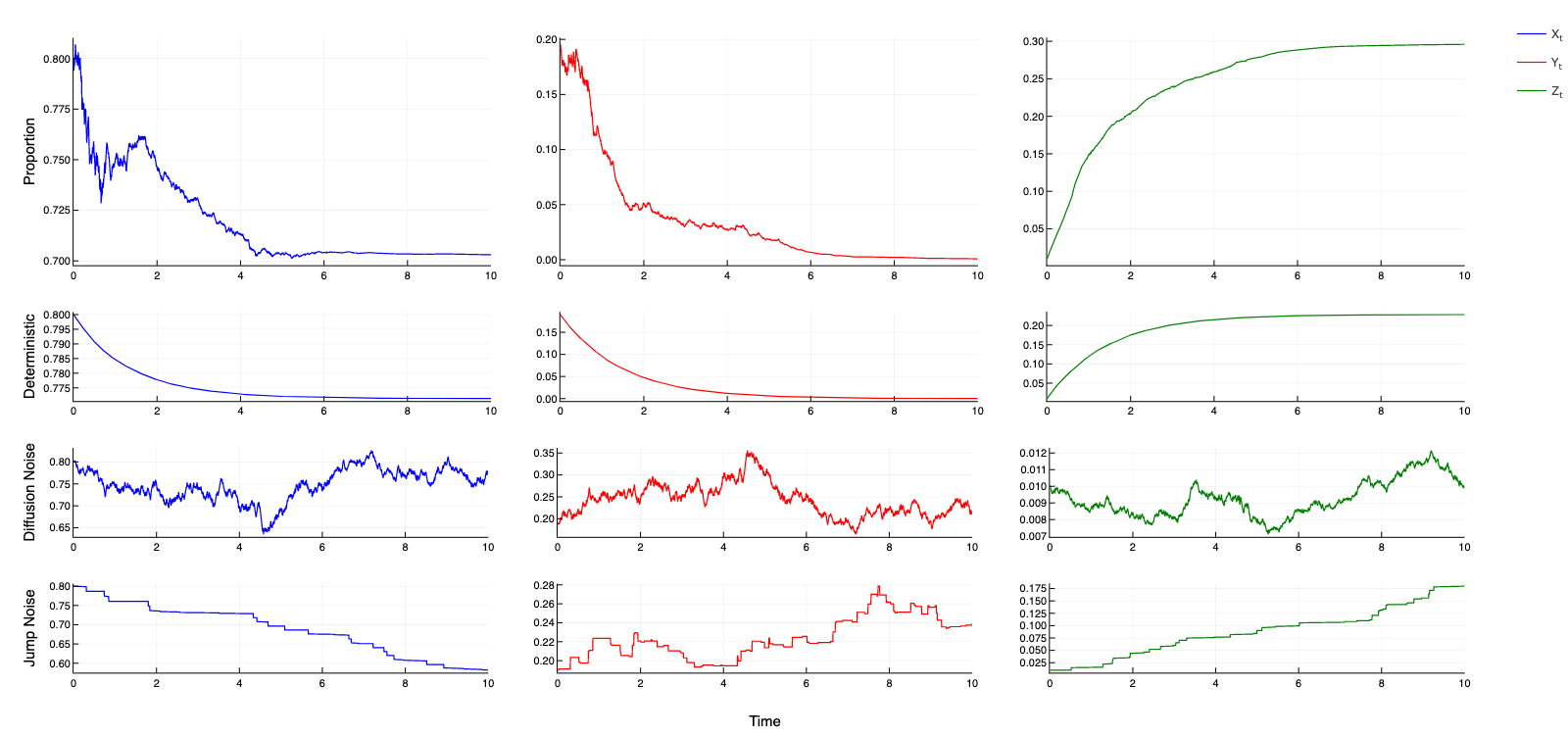
Figure 1: Row 1 gives a simulation of the stochastic simulation using E-M scheme of system (2.14), row 2 is the corresponding deterministic simulation, and rows 3 and 4 are the drift-free simulations of the diffusion and jump noise, respectively.

(ii)   We assume that the system (2.15) in Example 2.4(b) has initial values $(X_{0},Y_{0},Z_{0})=(0.85,0.1,0.05)$ and set the parameters in Table 2:

$f(t)$	$\underline{f}$	$\overline{f}$
$\beta(t)=0.17+0.01\cos(20t)$	$0.16$	$0.18$
$\gamma_{1}(t)=0.12+0.01\cos(t)$	$0.11$	$0.13$
$\gamma_{2}(t)=0.56+0.01\sin(t)$	$0.55$	$0.57$
$\sigma(t)=0.141+0.02(\sin(t)+\cos(t))$	$0.141-0.02\sqrt{2}$	$0.141+0.02\sqrt{2}$
$h_{1}(u)=0.019$	—	—
$h_{2}(u)=0.018$	—	—
$g_{1}(u)=0.11$	—	—
$g_{2}(u)=0.1$	—	—

Table 2: Parameters for simulation of system (2.15).

We achieve results which illustrate persistence of the disease, as is displayed in Figure 2 below. Furthermore, we have $\lambda_{0}=0.55$, $\lambda=0.0776367$ and

$$\liminf_{t\to\infty}\frac{1}{t}\int_{0}^{t}Y_{s}ds\geq\frac{0.0776367}{0.55}\geq 0.14115.$$

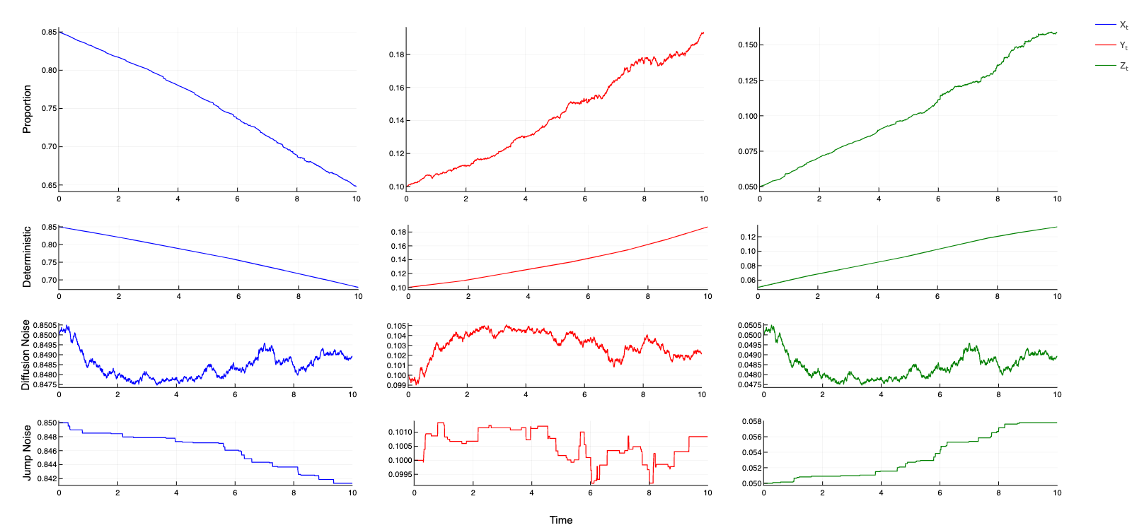
Figure 2: Row 1 gives a simulation of the stochastic simulation using E-M scheme of system (2.15), row 2 is the corresponding deterministic simulation, and rows 3 and 4 are the drift-free simulations of the diffusion and jump noise, respectively.

(iii)  The simulations are concerned with Example 3.3, system (3.3). The initial condition is set to $(X_{0},Y_{0},Z_{0})=\left(2.0,0.8,1\right)$, where the starting population is $3.8$ million. In the following simulations, the parameters will change to demonstrate their effects on a system with unchanging initial condition. The first two simulations illustrate extinction of the disease and the final simulation will illustrate persistence of the disease. We initially set the parameters in Table 3:

$f(t)$	$\underline{f}$	$\overline{f}$
$\beta(t)=0.13+0.01\sin(t)$	$0.12$	$0.14$
$\gamma(t)=0.9+0.02\sin(t)$	$0.88$	$0.92$
$\varepsilon(t)=0.15+0.07\sin(t)$	$0.08$	$0.22$
$\sigma(t)=0.12+0.01(\sin(t)+\cos(t))$	$0.12-0.01\sqrt{2}$	$0.12+0.01\sqrt{2}$
$\Lambda(t)=0.5+0.06\sin(t)$	$0.44$	$0.56$
$\mu(t)=0.07+0.004\cos(t)$	$0.066$	$0.074$

Table 3: Parameters for simulation 1 of system (3.3).

It is important to note that since the initial condition is unchanging this forces two parameters, namely $\Lambda(t)$ and $\mu(t)$, to remain unchanged for these simulation purposes. Moreover, we have that

$$\Gamma=\left\{(x,y,z)\in\mathbb{R}_{+}^{3}:x+y+z\leq\frac{\overline{\Lambda}}{\underline{\mu}}=8.484848\right\}$$

as the invariant set for the system (3.3). That is, this system has a unique strong solution taking values in $\Gamma$ per Theorem 3.1. Given these parameters and following Example 3.3, we have

$$\tilde{R}_{0}=\frac{\overline{\beta}\,\overline{\Lambda}}{\underline{\mu}(\underline{\mu}+\underline{\gamma}+\underline{\varepsilon})}-\frac{\underline{\sigma}^{2}\overline{\Lambda}^{2}}{2\underline{\mu}^{2}(\underline{\mu}+\underline{\gamma}+\underline{\varepsilon})}\ \leq 0.7646<1,\ \ \ \ \underline{\sigma}^{2}<0.0121<0.0165=\frac{\underline{\mu}\overline{\beta}}{\overline{\Lambda}}.$$

As demonstrated below in Figure 3, the disease will go extinct with exponential rate

$$-\alpha\geq(\underline{\mu}+\underline{\gamma}+\underline{\varepsilon})\left(1-\tilde{R}_{0}\right)\geq 0.241.$$

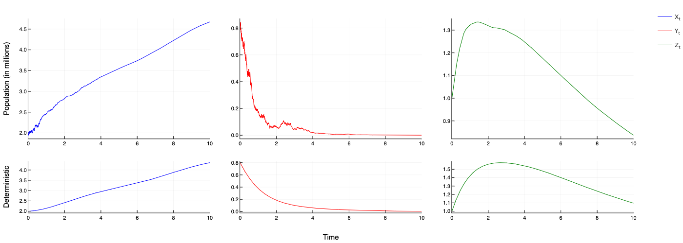
Figure 3: Row 1 is the E-M scheme simulation 1 of system (3.3) illustrating disease extinction and row 2 is the corresponding deterministic system.

We now make only the alteration of a single parameter in the system (3.3). Assume that $\sigma(t)$ has the form given in Table 4:

$f(t)$	$\underline{f}$	$\overline{f}$
$\sigma(t)=0.55+0.003(\sin(t)+\cos(t))$	$0.55-0.003\sqrt{2}$	$0.55+0.003\sqrt{2}$

Table 4: Parameters for simulation 2 of system (3.3).

This alteration yields

$$\underline{\sigma}^{2}\geq 0.29>0.0165\geq\max\left\{\frac{\underline{\mu}\overline{\beta}}{\overline{\Lambda}},\ \frac{\overline{\beta}^{2}}{2(\underline{\mu}+\underline{\gamma}+\underline{\varepsilon})}\right\}.$$

Thus, we have the scenario in which the disease goes extinct with exponential rate

$$-\alpha\geq(\underline{\mu}+\underline{\gamma}+\underline{\varepsilon})-\frac{\overline{\beta}^{2}}{2\underline{\sigma}^{2}}\geq 0.993.$$

Moreover, if we compare Figure 4 to the above Figure 3 we notice the disease appears to go extinct at a faster rate which is as expected given the above results.

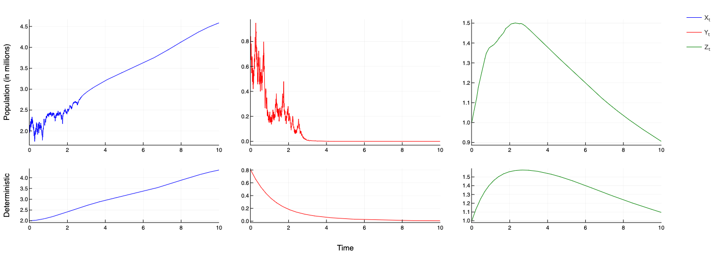
Figure 4: Row 1 is the E-M scheme simulation 2 of system (3.3) illustrating disease extinction and row 2 is the corresponding deterministic system.

Now assume that the parameters for the system (3.3) are given in Table 5:

$f(t)$	$\underline{f}$	$\overline{f}$
$\beta(t)=0.56+0.01\sin(4t)$	$0.55$	$0.57$
$\gamma(t)=0.25+0.1\cos(5t)$	$0.15$	$0.35$
$\sigma(t)=0.24+0.01(\sin(t)+\cos(t))$	$0.24-0.01\sqrt{2}$	$0.24+0.01\sqrt{2}$

Table 5: Parameters for simulation 3 of system (3.3).

This modification yields

$$\tilde{R}_{0}=\frac{\underline{\beta}\underline{\Lambda}}{\overline{\mu}(\overline{\mu}+\overline{\gamma}+\overline{\varepsilon})}-\frac{\overline{\sigma}^{2}\overline{\Lambda}^{2}}{2\underline{\mu}^{2}(\overline{\mu}+\overline{\gamma}+\overline{\varepsilon})}\geq 1.7>1.$$

In Figure 5 below, we see such a modification yields disease persistence as opposed to disease extinction achieved in the previous two simulations for the system (3.3).

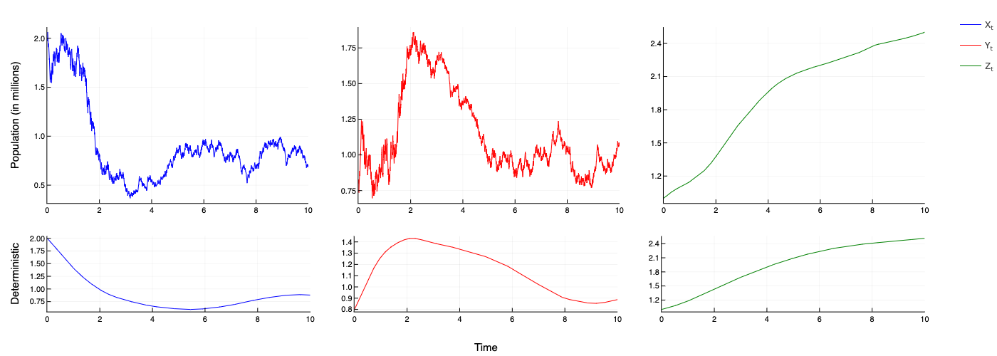
Figure 5: Row 1 is the E-M scheme simulation 3 of system (3.3) illustrating disease persistence and row 2 is the corresponding deterministic system.

(iv)   We assume the system (3.7) has initial conditions $(3.75,1.15,1.1)$, where the values are taken to be in millions. Set the parameters in Table $6$:

$f(t)$	$\underline{f}$	$\overline{f}$
$M=2$	—	—
$\Lambda(t)=0.15+0.006\sin(t)$	$0.144$	$0.156$
$\mu(t)=0.002+0.0001\cos(t)$	$0.0019$	$0.0021$
$\beta(t)=0.18+0.01\sin(2t)$	$0.17$	$0.19$
$\gamma_{1}(t)=0.15+0.004\cos(t)$	$0.146$	$0.154$
$\gamma_{2}(t)=0.12+0.02\cos(t)$	$0.1$	$0.14$
$\gamma_{3}(t)=0.12+0.04\cos(2t)$	$0.08$	$0.16$
$\gamma_{4}(t)=0.1+0.04\sin(4t)$	$0.06$	$0.14$
$\xi(t)=1+\ln(1+|\sin(t)|)$	$1$	$1+\ln 2$
$\varphi_{i}(t)=0.01+0.005\cos(t),i=1,2$	$0.005$	$0.015$
$\varphi_{3}(t)=1+0.25\sin(15t)$	$0.75$	$1.25$
$\sigma_{1}(t)=0.15+0.01\cos(t)$	$0.14$	$0.16$
$\sigma_{2}(t)=0.12+0.01\sin(t)$	$0.11$	$0.13$
$h_{1}(u)=0.0001$	—	—
$h_{2}(u)=0.00025$	—	—
$h_{3}(u)=0.0009$	—	—
$g_{1}(u)=0.001$	—	—
$g_{2}(u)=0.0012$	—	—

Table 6: Parameters for simulation of system (3.7).

We have $\lambda_{0}=1.16$ and $\lambda\geq 0.075$ and

$$\liminf_{t\to\infty}\frac{1}{t}\int_{0}^{t}Y_{s}ds\geq\frac{0.075}{1.16}\geq 0.064.$$

The resulting persistence of disease is illustrated below in Figure $6$.

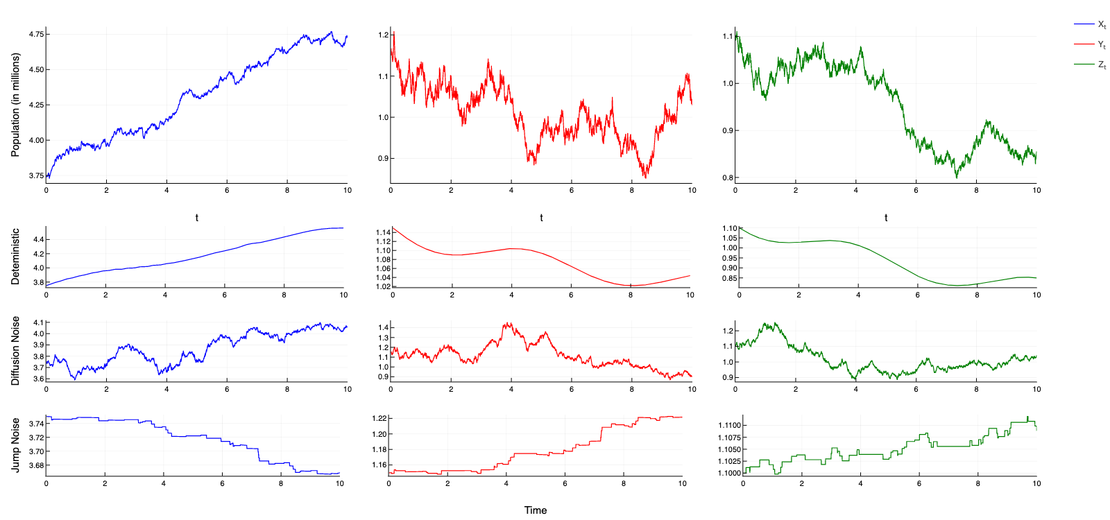
Figure 6: Row 1 gives E-M scheme simulation of system (3.7) illustrating disease persistence and subsequent rows give corresponding deterministic, diffusion noise and jump noise simulations, respectively.

(v)   We assume the system (3.8) has initial conditions $(7.27,1.5,1.11)$, where the values are taken to be in millions. Set the parameters in Table $7$:

$f(t)$	$\underline{f}$	$\overline{f}$
$M=1.5$	—	—
$\Lambda(t)=0.09+0.01\cos(t)$	$0.08$	$0.1$
$\mu(t)=0.003+0.001\sin(t)$	$0.002$	$0.004$
$\beta(t)=0.14+0.005\cos(10t)$	$0.135$	$0.145$
$\gamma_{1}(t)=0.002+0.002\cos(25t)$	$0$	$0.004$
$\gamma_{2}(t)=0.35+0.04\cos(15t)$	$0.31$	$0.39$
$\sigma(t)=0.3125+0.002(\sin(t)+\cos(t))$	$0.3125-0.002\sqrt{2}$	$0.3125+0.002\sqrt{2}$
$h_{1}(u)=0.0001$	—	—
$h_{2}(u)=0.0004$	—	—
$h_{3}(u)=0.0009$	—	—
$g_{1}(u)=0.001$	—	—
$g_{2}(u)=0.007$	—	—
$g_{3}(u)=0.005$	—	—

Table 7: Parameters for simulation of system (3.8).

The extinction of the disease is illustrated below in Figure $7$. Moreover, as in Example (3.4)(b), the disease will go extinct with rate $-\alpha\geq\underline{\gamma_{2}}+\underline{\mu}-\overline{\beta}-2\overline{g_{1}}\geq 0.165$.

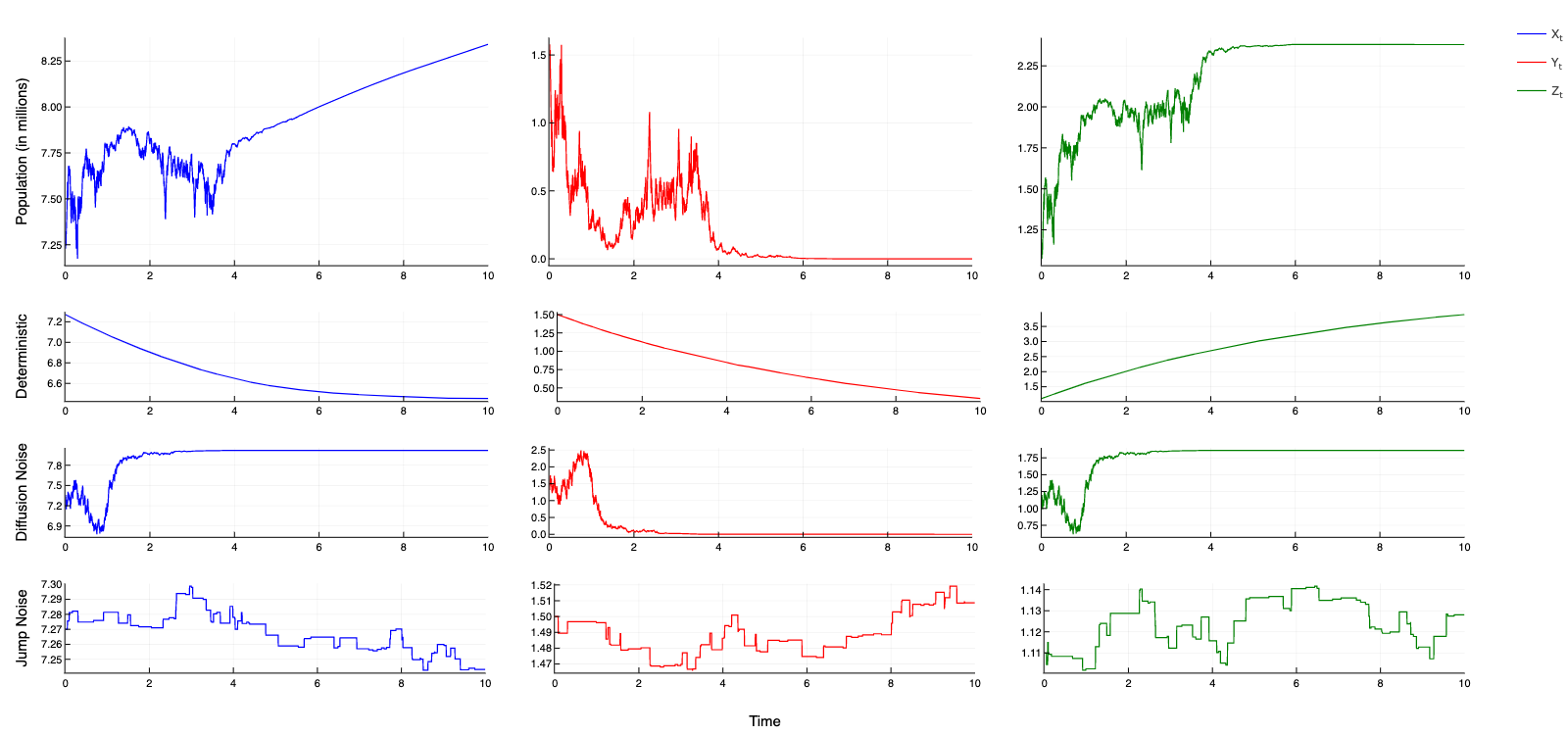
Figure 7: Row 1 gives E-M scheme simulation of system (3.8) illustrating disease extinction and subsequent rows give corresponding deterministic, diffusion noise and jump noise simulations, respectively.

5 Conclusion

In this paper, we propose and investigate the USSIR model given by the system (1.3). We have presented two forms of the novel model – one for population proportions and the other for population numbers. For both forms of the model, we have given results on the extinction and persistence of diseases; moreover, we have shown that these results still hold with time-dependent, nonlinear parameters and multiple Lévy noise sources. Notably, we give examples and simulations that agree with the theoretical results and illustrate the impact that noise has on a given SIR model system. Moreover, the ability to allow time-dependency and multiple noises coincides with real world occurrences of infectious disease spread due to environmental noises or time-dependent events such as temperature, climates, seasons, and so forth. The more general nature of the USSIR model allows for many tailored use cases which will be further explored in upcoming work.

References

- [1] D. Applebaum. Lévy Processes and Stochastic Calculus, Second Edition. Cambridge University Press (2009).
- [2] N. Bailey. The Mathematical Theory of Infectious Diseases and Its Applications, Second Edition. London: Griffin (1975).
- [3] J. Bao and C. Yuan. Stochastic population dynamics driven by Lévy noise. J. Math. Anal. Appl. 391, 363-375 (2012).
- [4] F. Brauer, C. Castillo-Chavez and Z. Feng. Mathematical Models in Epidemiology. Springer (2019).
- [5] T. Caraballo, M. El Fatini, M. El Khalifi and A. Rathinasamy. Analysis of a stochastic coronavirus (COVID-19) Lévy jump model with protective measures. Stoch. Anal. Appl. (2021).
- [6] G. Chen, T. Li and C. Liu. Lyapunov exponent of a stochastic SIRS model. Comp. Rend. Math. 351, 33-35 (2013).
- [7] N. Dalal, D. Greenhalgh and X. Mao. A stochastic model of AIDS and condom use. J. Math. Anal. Appl. 325, 36-63 (2007).
- [8] A. El Koufi, J. Adnani, A. Bennar and N. Yousfi. Analysis of a stochastic SIR model with vaccination and nonlinear incidence rate. Int. J. Diff. Equ. 9275051 (2019).
- [9] A. El Koufi, J. Adnani, A. Bennar and N. Yousfi. Dynamics of a stochastic SIR epidemic model driven by Lévy jumps with saturated incidence rate and saturated treatment function. Stoch. Anal. Appl. (2021).
- [10] C. Gourieroux and Y. Lu. SIR model with stochastic transmission. arXiv:2011.07816 (2020).
- [11] A. Gray, D. Greenhalgh, L. Hu, X. Mao and J. Pan. A stochastic differential equation SIS epidemic model. SIAM J. Appl. Math. 71, 876-902 (2011).
- [12] X-X. Guo and W. Sun. Periodic solutions of stochastic differential equations driven by Lévy noises. J. Nonl. Sci. 31:32 (2021).
- [13] C. Ji and D. Jiang. Threshold behaviour of a stochastic SIR model. Appl. Math. Modell. 38, 5067-5079 (2014).
- [14] C. Ji, D. Jiang and N. Shi. Multigroup SIR epidemic model with stochastic permutation. Physica A. 390, 1747-1762 (2011).
- [15] W. Kermack and A. McKendrick. Contributions to the mathematical theory of epidemics. Proc. R. Soc. Lond. Ser. A. 115, 700-721 (1927).
- [16] R. S. Liptser and A.N. Shiryayev. Theory of Martingales. Kluwer Academic Publishers (1986)
- [17] Y. Liu, Y. Zhang and Q-Y. Wang. A stochastic SIR epidemic model with Lévy jump and media coverage. Adv. Diff. Equ. 70 (2020).
- [18] N. Privault and L. Wang. Stochastic SIR Lévy jump model with heavy-tailed increments. J. Nonlin Sci. 31:15 (2021).
- [19] R. Schlickeiser and M. Kröger. Analytical modeling of the temporal evolution of epidemics outbreaks accounting for vaccinations. Physics 3, 386-426 (2021).
- [20] E. Tornatore, S. Buccellato and P. Vetro. Stability of a stochastic SIR system. Physica A. 354, 111-126 (2005).
- [21] X. Zhang and K. Wang. Stochastic SIR model with jumps. Appl. Math. Lett. 26, 867-874 (2013).
- [22] Y. Zhou, S. Yuan and D. Zhao. Threshold behavior of a stochastic SIS model with Lévy jumps. Appl. Math. Comp. 275, 255-267 (2016).
- [23] Y. Zhou and W. Zhang. Threshold of a stochastic SIR epidemic model with Lévy jumps. Physica A. 446, 204-216 (2016).