BeyondPlanck X. Bandpass and beam leakage corrections

We discuss the treatment of bandpass and beam leakage corrections in the Bayesian BeyondPlanck CMB analysis pipeline as applied to the Planck LFI measurements. As a preparatory step, we first apply three corrections to the nominal LFI bandpass profiles including removal of a known systematic effect in the ground measuring equipment at 61 GHz; smoothing of standing wave ripples; and edge regularization. The main net impact of these modifications is an overall shift in the 70 GHz bandpass of +0.6 GHz; we argue that any analysis of LFI data products, either from Planck or BeyondPlanck, should use these new bandpasses. In addition, we fit a single free bandpass parameter for each radiometer of the form $\Delta_{i}=\Delta_{0}+\delta_{i}$, where $\Delta_{0}$ represents an absolute frequency shift per frequency band and $\delta_{i}$ is a relative shift per detector. The absolute correction is only fitted at 30 GHz with a full $\chi^{2}$-based likelihood, resulting in a correction of $\Delta_{30}=0.24\pm 0.03\thinspace$GHz. The relative corrections are fitted using a spurious map approach, fundamentally similar to the method pioneered by the WMAP team, but without introducing many additional degrees of freedom. All bandpass parameters are sampled using a standard Metropolis sampler within the main BeyondPlanck Gibbs chain, and bandpass uncertainties are thus propagated to all other data products in the analysis. In total, we find that our bandpass model significantly reduces leakage effects. For beam leakage corrections, we adopt the official Planck LFI beam estimates without additional degrees of freedom, and only marginalize over the underlying sky model. We note that this is the first time leakage from beam mismatch has been included for Planck LFI maps.

1 Introduction

The cosmic microwave background (CMB), first discovered by Penzias & Wilson (1965) is one of the most important sources of information in cosmology. The most recent full-sky measurements of this signal were made by the Planck satellite (Planck Collaboration I 2020) from an orbit around the second Sun-Earth Lagrange point between 2009 and 2013, using two complementary instruments to observe the sky in nine frequency bands between 30 and 857 GHz. These measurements have put strong constraints on a wide range of both cosmological parameters and physical phenomena, and form one of the cornerstones of contemporary cosmology.

Although the official Planck data processing ended in 2020 (Planck Collaboration I 2020; Planck Collaboration Int. LVII 2020), several open questions regarding low-level instrumental effects in Planck remained unanswered at that time. Addressing these for the Low Frequency Instrument (LFI; Planck Collaboration II 2020) is a main motivation for the BeyondPlanck project (BeyondPlanck 2022). The BeyondPlanck machinery is unique in that it processes raw time ordered data (TOD) into final cosmological and astrophysical results within one single integrated end-to-end Bayesian analysis framework. Its computational engine is Commander (Eriksen et al. 2004, 2008; Galloway et al. 2022), which was originally developed for Planck component separation purposes (Planck Collaboration XII 2014; Planck Collaboration X 2016; Planck Collaboration IV 2018), and uses Gibbs sampling (Geman & Geman 1984) to draw samples from a large global posterior distribution. The BeyondPlanck project has generalized this code to also account for low-level data processing and mapmaking, and thereby integrated the full analysis pipeline into a self-consistent Bayesian framework. For a full description of the BeyondPlanck project, we refer the interested reader to BeyondPlanck (2022).

A defining theme for the BeyondPlanck approach is a detailed statistical exploration of the interplay between instrumental effects and astrophysical foregrounds. Particularly relevant in this respect are spectral responses. LFI comprised 22 radiometer chain assemblies (RCAs) grouped in three bands with nominal frequencies of 30, 44 and 70 GHz. Within a band, each RCA has a slightly different spectral response (or bandpass profile) and center frequency compared to the others. The Planck LFI spectral responses used in the official analysis were provided as part of the 2018 data release. These response functions were measured on the ground prior to launch, as described by Zonca et al. (2009). However, laboratory measurements of bandpass profiles are in general a highly non-trivial task, as even small environmental variations and interferences may affect the results. Several systematic issues were identified during the LFI testing campaign, and some of these were left uncorrected in the final LFI products, even though approaches for possible improvements were discussed. In this paper, we finally implement these corrections, and make the resulting bandpass profiles publicly available. We also recommend that any future analysis of the Planck LFI data should use the new bandpasses, as the effects are non-negligible and lead to improved internal consistency.

Even with perfect knowledge of the instrument, there will be artefacts in the final frequency and component maps when using a multi-detector mapmaking algorithm (which includes those employed by Planck; Planck Collaboration II 2020; Planck Collaboration III 2020) if the detectors have different sensitivities, unless these differences are properly accounted for (e.g., Page et al. 2007; Planck Collaboration Int. LVII 2020; Delouis et al. 2019). This applies both to differences in bandpass and beam profiles. In this paper, we discuss how such corrections are applied within the BeyondPlanck framework, both in terms of how to correct deterministically for an assumed known response functions, and how to account for uncertainties in the response functions themselves.

We note that for the white noise levels typical of WMAP and Planck, previous static leakage corrections suppress residual effects well below the levels relevant for cosmological interpretation. However, future CMB experiments will target primordial gravitational waves (e.g., (Kamionkowski & Kovetz 2016) and references therein) and more specifically the tensor-to-scalar ratio, $r$. Current measurements from BICEP2/Keck and Planck constrain this parameter to $r<0.036$ (Ade et al. 2021) and $r<0.032$ (Tristram et al. 2021), respectively, and these low levels correspond to signals that are only a few hundreds of nanokelvin on the sky. To reach levels of $r\lesssim 10^{-3}-10^{-4}$, highly accurate modelling of bandpass and beam leakage effects will be critically important, and we believe that an integrated method of the kind shown in this paper will be required.

The rest of this paper is organized as follows. We start by discussing the LFI bandpass pre-processing in Sect. 2. We then present our own algorithms in Sect. 3, and show how these directly build on and generalize previous efforts. Results from the main Markov chain analysis are reported in Sect. 4, and we finally conclude in Sect. 5.

2 Bandpass pre-processing

We start our discussion by reviewing the bandpass profiles provided by the official Planck LFI data processing center (DPC) (Planck Collaboration II 2014), as shown in Fig. 1 for each radiometer. As summarized by Zonca et al. (2009), these functions were characterized through two complementary approaches. The first was to model and characterize each optical element individually, and then combine these into a complete model. The second approach was through integrated cryogenic system tests, which for LFI were carried out by Thales Alenia Space in Vimodrone for the 30 and 44 GHz channels, and by DA-Design Ylinen in Finland for the 70 GHz channel.

While the results from the two approaches generally agreed, there were also notable differences, some of which may be identified by eye in Fig. 1. Perhaps the most striking feature is standing waves, which result in high-frequency ripples across the bandpass. While some of these may be due to real features in RCA itself, others may be caused by standing waves excited by the testing equipment. One particularly notable example of this is the 70 GHz channel, for which the input load was placed directly in front of the feed horn during the test, resulting in strong standing waves between the two components. At the same time, the precise phase of the ripples is sensitive to environmental properties, and can for instance change depending on the ambient temperature. As such, it is non-trivial to assign a physical reality to these ripples as far as the real measurements are concerned. Zonca et al. (2009) therefore suggested that these should be removed through low-pass filtering before cosmological data analysis. This step was, however, never actually implemented during the official Planck analysis, and we therefore do this in this paper. Technically speaking, we implement this filter in logarithmic space using a 3-pole low pass filter at 0.2 times the Nyquist frequency. We note, however, that the specific details regarding the filter are not critically important.

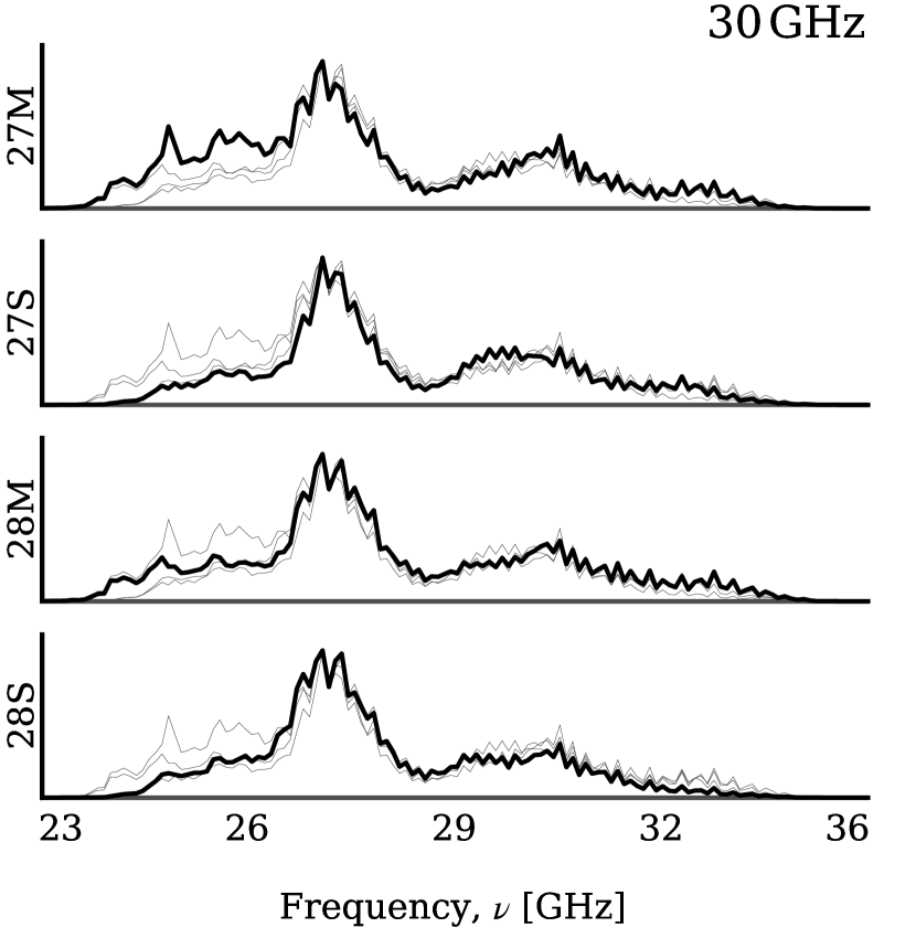
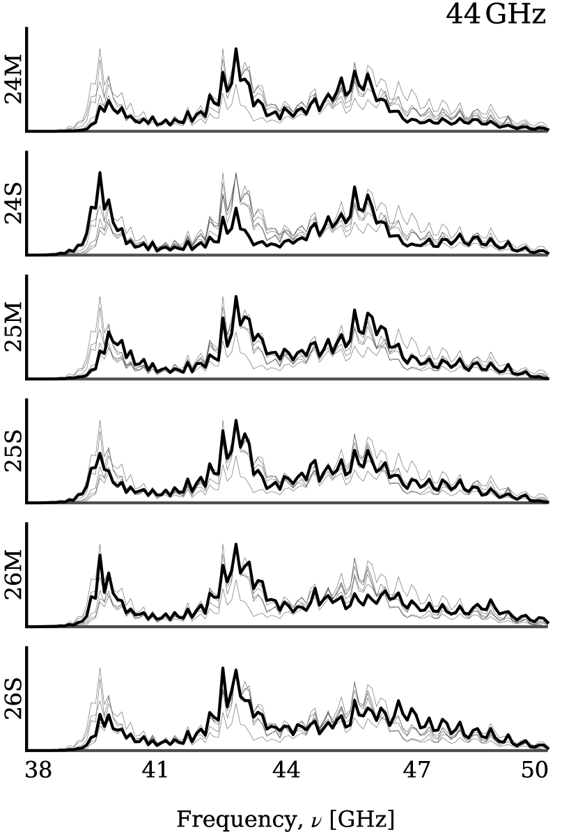
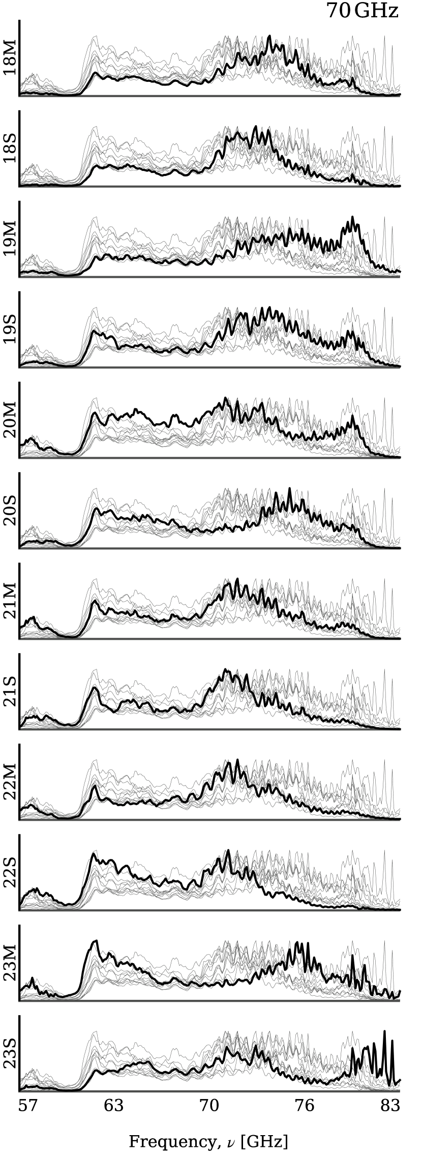
Figure 1: Normalized radiometer bandpass profiles for LFI 30 GHz (top left), 44 GHz (bottom left), and 70 GHz (right). Individual bandpasses are highlighted in bold and the remaining are plotted behind for ease of comparison.

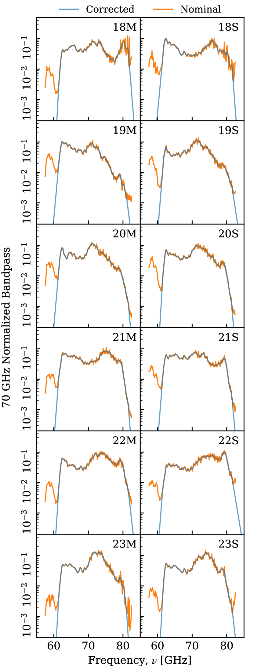
Figure 2: Nominal and corrected bandpass profiles for LFI 30 GHz (top left), 44 GHz (bottom left), and 70 GHz (right) radiometers. Orange curves show raw bandpass profiles as provided by the Planck LFI DPC, and blue curves show the corrected profiles discussed in Sect. 2.

A second known artefact induced by the testing equipment is the excess seen in the 70 GHz bandpasses below 61 GHz, which is due to a known systematic effect in all gain measurements of the backend module (BEM); it is thus caused by the test equipment, and not the radiometers themselves (Zonca et al. 2009). This feature should simply be removed, and the 70 GHz bandpass should be limited to 61–80 GHz.

Table 1: Effective center frequencies, $\nu_{\rm eff}$, and unit conversion factors, $U_{c}$, for nominal and corrected bandpass profiles.

Quantity $$\rm Unit$$ %

.

.

.

More generally, the edges of the bandpasses are not well characterized, and standing wave effects also tend to be relatively larger near the edges. The bandpass cut-offs should therefore be regularized through smooth apodization. In this paper, we implement this by calculating the derivative of the low-pass filtered profiles near the edges, and extrapolate smoothly to zero. For the 70 GHz channel, the derivative is evaluated at 61 GHz to remove the BEM artefact discussed above.

Figure 2 shows a comparison of the raw and corrected bandpasses for each radiometer. Here we see that the main change applied to the 30 GHz radiometers is the low-pass filter, as the edges were already quite well characterized in the original measurements. For the 44 GHz band, the most prominent correction is the high frequency cutoff. In particular, extrapolating the behavior for horn 24 is not trivial, as the profiles do not show a convincing downward trend before truncation. However, the profiles for both horn 25 and 26 suggest that the power drop-off is most likely just outside the measured range.

Edge trimming is also the dominant effect for the 70 GHz channels, both at low and high frequencies. The substantial amplitude and width of the 61 GHz spike feature implies that even the center frequency of the 70 GHz channel will change notably for this channel. This is quantified in Table 1; see next section for exact definitions of each quantity. Here we see that the 70 GHz center frequency increases by 0.44 GHz or, equivalently, by 0.6 %, which translates into a difference in the conversion factor between flux density and thermodynamic temperature units, $U_{c}$, of 2.5 %. The impact of these corrections in terms of data quality and astrophysical products is considered in Sect. 4. The Python script that applies the various corrections is available online.

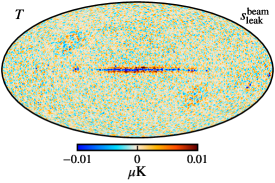
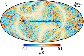
Figure 3: Comparison of the raw (top row) and leakage corrected (second row) Planck 30 GHz channel. The third and fourth rows show the individual bandpass and beam leakage corrections, respectively. Columns shows Stokes $T$, $Q$, and $U$ parameters. All maps have been smoothed to an angular resolution of 1^∘ FWHM, except for the bottom row, which has been smoothed to 2^∘ FWHM.

Figure 4: (Top left:) Gnomonic projection of a $30^{\circ}\times 30^{\circ}$ area centered on $(l,b)=(0^{\circ},-70^{\circ})$ in the BeyondPlanck posterior mean CMB temperature map (Colombo et al. 2022). (Top right:) BeyondPlanck 44 GHz $Q$-leakage map in the same area. (Bottom:) Angular polarization power spectra of the masked 44 GHz leakage map, compared with the Planck best-fit $\Lambda$CDM $TT$ (scaled by $10^{-3}$) and $EE$ spectra.

3 Methodology

The main goal of the BeyondPlanck project is to perform an end-to-end Bayesian analysis of the Planck LFI data. To do so, we start by writing down a physically motivated parametric model which can be fitted to our calibrated time-ordered data, $\@vec{d}$ for radiometer $j$,

$$\@vec{d}_{j}=\@tens{P}_{j}\@tens{B}_{j}\int\@vec{s}(\nu)\tau_{j}(\nu)\thinspace\mathrm{d}\nu+\@vec{n}_{j}.$$ (1)

Here $\@tens{P}$ is a pointing matrix that maps the sky signal $\@vec{s}$ into time domain; $\@tens{B}$ is the beam profile; and $\tau(\nu)$ is the bandpass. The sky signal as observed by radiometer $j$ may be written in the following form,

$$\@vec{s}^{j}=\sum_{c=1}^{N_{\mathrm{comp}}}\@vec{a}_{c}\thinspace\left[\thinspace U_{j}\int f_{c}(\nu;\beta)\thinspace\tau_{j}(\nu)\thinspace\mathrm{d}\nu\right]\equiv\sum_{c=1}^{N_{\mathrm{comp}}}\@tens{M}^{j}_{c}\thinspace\@vec{a}_{c}=\@tens{M}^{j}\thinspace\@vec{a},$$ (2)

where the sum runs over all relevant astrophysical sky components, $c$, each with its own unit conversion factor $U_{j}$ that converts from its own intrinsic unit to the common brightness temperature unit adopted for $\@vec{s}$. As shown by (Planck Collaboration IX 2014), this may be written as

$$U_{ij}=\frac{\int\tau(\nu)\frac{dI_{\nu}}{dX_{i}}\thinspace\mathrm{d}\nu}{\int\tau(\nu)\frac{dI_{\nu}}{dX_{j}}\thinspace\mathrm{d}\nu},$$ (3)

where $dI_{\nu}/dX_{i}$ is the intensity derivative expressed in the given unit convention.

As defined by Eq. (2), $\@tens{M}_{c}^{j}$ is called the mixing matrix, and this matrix scales the set of component amplitudes $\@vec{a}$ to arbitrary frequencies using the spectral energy distribution $f$ of each component, which may be described by some set of spectral parameters $\beta$. Using this notation, Eq. (1) be written in the following slightly more compact form,

$$\@vec{d}_{j}=\@tens{P}_{j}\@tens{B}_{j}\@tens{M}_{j}\@vec{a}+\@vec{n}_{j}.$$ (4)

For a full discussion of the BeyondPlanck data model and notation, we refer the interested reader to BeyondPlanck (2022) and references therein.

In this paper, we are particularly interested in how beam and bandpass differences between detectors create leakage effects, and how to correct for these. The first complication in that respect is related to binning the time-ordered data, $\@vec{d}$, into Stokes parameter maps, $\@vec{m}_{\nu}$, using the mapmaking equation,

$$\left(\sum_{j\in\nu}\@tens{P}_{j}^{t}\@tens{N}_{j}^{-1}\@tens{P}_{j}\right)\@vec{m}_{\nu}=\sum_{j}\@tens{P}_{j}^{t}\@tens{N}_{j}^{-1}\@vec{d}_{j},$$ (5)

where we now have defined $\@tens{N}_{j}=\left<\@vec{n}\@vec{n}^{t}\right>$ to be the (time-domain) noise covariance matrix for detector $j$.

This equation implicitly assumes that all radiometers, $j$, observe the same sky, $\@vec{s}$. However, although the various detectors actually do observe the same sky, their response to the spectral distribution of the different foreground components varies, because the bandpass and beam profiles differ, as described by Eq. (1). When co-adding these different measurements into a sky map, any difference from the mean will be interpreted as noise by the mapmaker, and accordingly be distributed between the various Stokes parameters according to the local scanning and noise levels at any given time. Furthermore, since these discrepancies are not stochastic, but deterministically predictable by the bandpass and beam profiles, they do not average down in time. They therefore induce systematic errors in the final maps that are directly correlated with the sky signal itself. These effects are particularly significant for polarization analysis, where different bands must be combined to extract the very low Q and U signals. These errors are therefore particularly worrisome for cosmological and astrophysical analyses.

We define three different effects caused by bandpass and beam errors. The first effect is called bandpass mismatch, and this describes the deterministic effect discussed above, namely that different bandpass profiles create spurious leakage during multi-detector mapmaking, creating what is often referred to as “temperature-to-polarization leakage”. However, this name is somewhat of misnomer, since all Stokes parameters are formally coupled (see, e.g., Planck Collaboration Int. LVII 2020). Still, the effect is relatively much more important for polarization than for temperature because of its far lower signal-to-noise ratio. Indeed, this effect is the single strongest instrumental polarization contaminant for the LFI 30 GHz channel (see, e.g., Fig. 16 in BeyondPlanck 2022), but, fortunately, it is also entirely predictable, and could in principle be removed to machine accuracy if both the astrophysical sky and the detector bandpasses were perfectly known.

However, as discussed above, the bandpasses are by no means perfectly known, and those uncertainties create additional leakage that is not deterministically correctable. Furthermore, since all radiometer bandpasses within a band are uncertain, the combined co-added frequency bandpass is also uncertain. And this uncertainty produces an artefact when incorrectly translating the foreground sky model to the observed signal through the mixing matrix in Eq. (2). We refer to the effect caused by bandpass uncertainties as bandpass errors, and we attempt to minimize and marginalize over these by parameterizing the bandpasses, and fit the associated free parameters as part of the main Gibbs sampling process.

The third and final leakage effect considered here is beam mismatch, which is a deterministic leakage effect arising from differences between the main beams of the radiometers in a given frequency channel. These are in principle similar to the bandpass mismatch effect, but typically only affect small angular scales. In this paper we will only account for static FWHM differences between radiometers, but not asymmetric beams—that will be discussed in future publications, as will beam errors, i.e., uncertainties in the actual beam profiles.

3.1 Leakage corrections

As discussed above, bandpass mismatch artefacts arise because Eq. (5) assumes that all radiometers measure the same signal in any given pixel of the sky, while, they do not, because their different bandpass and beam profiles couple differently with the SED of foreground emissions. To account for these differences, we define the following leakage correction term for each radiometer,

$$\delta s^{\mathrm{leak}}_{j,t}=\@tens{P}^{j}_{tp}\@tens{B}_{pp^{\prime}}^{j}\left(s^{\mathrm{sky}}_{jp^{\prime}}-\left<s^{\mathrm{sky}}_{jp^{\prime}}\right>\right).$$ (6)

Here, $s^{\mathrm{sky}}_{j}$ is a model of the sky as actually seen by radiometer $j$ at pixel $p$, taking into account its specific bandpass and beam profile, and angled brackets denote an average over all radiometers evaluated pixel-by-pixel. Note that this leakage term explicitly accounts for both bandpass and beam differences through $s^{\mathrm{sky}}_{j}$ and $\@tens{B}_{pp^{\prime}}^{j}$.

In order to create a leakage-cleaned frequency map, we simply subtract this leakage term from the calibrated data prior to mapmaking,

$$\left(\sum_{j\in\nu}\@tens{P}_{j}^{t}\@tens{N}_{j}^{-1}\@tens{P}_{j}\right)\@vec{m}_{\nu}=\sum_{j\in\nu}\@tens{P}_{j}^{t}\@tens{N}_{j}^{-1}(\@vec{d}_{j}-\delta\@vec{s}^{\mathrm{leak}}_{j}).$$ (7)

In this equation, the right-hand side corresponds to a stationary sky signal in which all radiometers see the same effective sky signal, defined by the mean over all detectors, while the mean itself is not affected by the leakage correction, since $\delta\@vec{s}^{\mathrm{leak}}_{j}$ sums to zero by construction.

These corrections are conceptually similar to those applied by the Planck LFI DPC (Planck Collaboration II 2016, 2020) and Planck DR4 (Planck Collaboration Int. LVII 2020) pipelines, although implementation-wise they differ significantly from both. Firstly, neither of the two previous pipelines apply any beam leakage correction, while in the current work we account for the different beam FWHMs for each radiometer (Planck Collaboration III 2016) when evaluating Eq. (6). Secondly, while both of the previous pipelines use a linear approximation to the component SEDs to evaluate bandpass effects, we evaluate the full integral in Eq. (2) for each case, as described in Galloway et al. (2022). Thirdly, while the DPC pipelines makes separate maps for the raw TOD and the leakage correction, and subtract the latter as a post-processing step, we apply the corrections directly in time-domain prior to mapmaking, as does Planck DR4. Fourthly, while the DPC approach does not make any direct adjustments to the bandpass profiles themselves, we fit a parametric function for each of these, as described in the next section as part of the larger sampling framework, and thereby achieve a better overall fit. The Planck DR4 achieves a similar goal by fitting separate sky signal template terms for the mean and derivative of the foreground SED evaluated at the center frequency as part of their generalized mapmaker (Planck Collaboration Int. LVII 2020). Finally, neither of the previous pipelines allow for uncertainties in the astrophysical sky model itself, but rather adopts a Commander sky model as a static conditional input.

Figure 3 shows as comparison between the uncorrected (top row) and leakage corrected (second row) LFI 30 GHz map, as well as the individual contributions from bandpass leakage corrections (third row) and beam leakage corrections (bottom row). Comparing these maps, we immediately see that the bandpass leakage corrections are highly significant along the Galactic plane, with order unity corrections. Indeed, the corrections are sufficiently large that the central Galactic plane switches sign in both Stokes $Q$ and $U$. This makes any estimates of spectral parameters highly dependent on the leakage corrections, and joint estimation of both leakage corrections and spectral parameters is essential; for a specific discussion of Bayesian estimates of the spectral index of polarized synchrotron emission, see Svalheim et al. (2022). Likewise, the bandpass leakage corrections at high Galactic latitudes are dominated by the foreground monopoles, most notably those of synchrotron, AME and free-free emission, and consistent and joint estimation of monopoles and leakage corrections is therefore essential for large-scale CMB extraction. A novel feature of the BeyondPlanck processing is component-based monopole determination, which allows more easily self-consistent zero-level estimation across frequencies; for a discussion of this approach, see Andersen et al. (2022).

Comparing the bottom two rows of Fig. 3, it is visually obvious that the bandpass corrections are generally much more important than the beam errors on large angular scales. However, the beam corrections can also be important for CMB power spectrum analysis on smaller angular scales. This is illustrated in Fig. 4, which shows a $30^{\circ}\times 30^{\circ}$ zoom-in of the 44 GHz leakage correction map (top right panel) near the Galactic South Pole. This effect is particularly strong for the 44 GHz channel, because one of its three feeds (horn 24) has a significantly smaller beam width ($24{{}^{\scriptstyle\prime}}$ FWHM) than the other two (horns 25 and 26; $30{{}^{\scriptstyle\prime}}$ FWHM), as reported by Planck Collaboration IV (2016).

In this plot, we see that the spurious beam-induced small-scale polarization fluctuations are typically at a level of 1–2 $\mu$K. In addition, these fluctuations are primarily seeded by CMB temperature fluctuations, as seen by comparing the top two panels. The in-set circle provides a visual guide that makes it easy to identify correlations by eye. These spurious temperature-to-polarization leakage fluctuations induce spurious small-scale polarization modes. The bottom panel in Fig. 4 compares the angular power spectrum of the 44 GHz channel with the Planck 2018 best-fit $\Lambda$CDM $EE$ spectrum, as well as a scaled version of the $TT$ spectrum. Not only can uncorrected beam leakage correction confuse $EE$ and $BB$ measurements, but they can also obviously be a significant contaminant for $TE$, $TB$ and $EB$ correlations, and thereby contaminate constraints on both standard and non-standard physics, for instance gravitational lensing (e.g., Planck Collaboration Int. XLI 2016) or birefringence (e.g., Minami & Komatsu 2020).

3.2 Monte Carlo sampling of parametric bandpass models

Since each radiometer bandpass is measured with non-negligible uncertainties, our leakage correction model as defined by Eq. (6) is not perfect. For instance, as discussed in Sect. 2 the modifications made to the 70 GHz bandpasses in this paper changes its overall center frequency by 0.6 %, and this is likely to have a non-trivial impact on foreground estimates derived from these data, whereas relative measurement errors between individual detectors will create bandpass leakage as discussed above.

It is therefore important to parameterize the bandpasses themselves, fit the free parameters to the data, and marginalize over the corresponding uncertainties. Obviously, bandpasses have an indefinite number of degrees of freedom, being essentially free functions of frequency, and flight data are far from sufficient to constrain these frequency-by-frequency. It is therefore customary to base parametric models on the laboratory measurements, $\tau_{0}$, and only apply relatively mild corrections to these. For instance, Planck Collaboration X (2016) introduced a simple linear shift model,

$$\tau(\nu)=\tau_{0}(\nu+\Delta_{\mathrm{bp}}),$$ (8)

where $\Delta_{\mathrm{bp}}$ denotes a linear shift in frequency space. Another possible model is a power-law tilt model,

$$\tau(\nu)=\tau_{0}(\nu)\thinspace\left(\frac{\nu}{\nu_{\mathrm{c}}}\right)^{n},$$ (9)

where $\nu_{\mathrm{c}}$ is the center frequency, and $n$ is a spectral index. We have implemented support for both models in our codes, but we will focus only on the linear shift model in the following, as we generally find that the impact of the tilt model is too small for physically reasonable values of $n$ to have a relevant impact in terms of total map-level corrections.

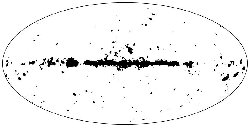
Figure 5: Mask used for bandpass correction sampling. The accepted sky fraction is $f_{\mathrm{sky}}=0.953$.

For the linear shift model, we split the total shift for radiometer $j$ into two components,

$$\Delta_{\mathrm{bp}}^{j}=\bar{\Delta}_{\mathrm{bp}}+\delta_{\mathrm{bp}}^{j}.$$ (10)

Here, $\bar{\Delta}_{\mathrm{bp}}$ corresponds to an absolute frequency shift for the overall co-added frequency band, while $\delta_{\mathrm{bp}}^{j}$ is a relative frequency shift for radiometer $j$ only, with the constraint that $\sum_{j}\delta_{\mathrm{bp}}^{j}=0$.

Absolute and relative bandpass corrections generally have very different impacts on the final sky maps. Intuitively, an absolute frequency shift can be interpreted as a “foreground-only calibration change”, in the sense that each foreground component becomes either weaker or brighter in the given frequency channel. The archetypal signature of an absolute bandpass error is that the residual map ($\@vec{d}_{\nu}-\@vec{s}_{\nu}$) shows an imprint of the Galactic plane, but there is no corresponding imprint of a residual CMB dipole; if there are both a CMB dipole and a Galactic plane imprint, then the problem is an absolute gain error. In contrast, relative bandpass errors primarily lead to temperature-to-polarization leakage, as visualized in Fig. 3, with a pattern defined by the Galactic intensity foregrounds modulated by the scanning strategy and polarization angle of the experiment in question.

Based on these observations, we employ different sampling techniques for $\bar{\Delta}_{\mathrm{bp}}$ and $\delta_{\mathrm{bp}}^{j}$, each with its own likelihood and proposal density. In both cases, however, we employ a standard Metropolis MCMC sampler with a tuned covariance matrix (see Appendix A in BeyondPlanck 2022), and we sample the absolute and relative corrections separately and alternately in each main Gibbs step; this interleaved sampling is exclusively for convenience of implementation, as the code becomes simpler by considering one type of corrections at any given time.

3.3 Absolute bandpass sampling

To derive a likelihood for the $\bar{\Delta}_{\mathrm{bp}}$ parameter, we note that this parameter conditionally only affects the sky signal model through the mixing matrix in Eq. (2), and we may therefore form the following data-minus-signal residual,

$$\@vec{r}_{\nu}=\@vec{d}_{\nu}-s_{\nu}(\bar{\Delta}_{\mathrm{bp}}),$$ (11)

where

$$\@vec{s}_{\nu}=\sum_{c}\@tens{M}_{cj}(\beta,\Delta_{\mathrm{bp}}^{j})\@vec{a}^{c}.$$ (12)

Under the assumption that $\@vec{r}_{\nu}$ may be modelled as Gaussian noise, as per Eq. (1), this results in a log-likelihood of the following form,

$$-2\ln\mathcal{L}(\bar{\Delta}_{\mathrm{bp}})=(\@vec{d}_{\nu}-s_{\nu}(\bar{\Delta}_{\mathrm{bp}}))^{T}\@tens{N}_{\nu}^{-1}(\@vec{d}_{\nu}-s_{\nu}(\bar{\Delta}_{\mathrm{bp}}))=\chi^{2}(\bar{\Delta}_{\mathrm{bp}}),$$ (13)

up to an irrelevant constant. Absolute bandpass sampling is thus equivalent to a standard $\chi^{2}$ fit, and one may sample from the corresponding conditional distribution through standard Metropolis MCMC with an accept rate of

$$a=\mathrm{min}(1,e^{-\frac{1}{2}(\chi^{2}_{i+1}-\chi^{2}_{i})}).$$ (14)

In practice, we apply a Galactic mask in these evaluations by setting $N_{p}^{-1}=0$ for masked pixels. However, since the calibration signal in question is precisely the Galactic plane, it is desirable to include as much of the sky as possible, and we only exclude the central parts of the Milky Way (within which foreground modelling is very complicated), as well as particularly bright points sources, such as Tau-A. The actual mask used is shown as a black region in Fig. 5, and excludes 4.7 % of the sky.

Finally, following Planck Collaboration X (2016), we will only estimate an absolute correction for the LFI 30 GHz channel. Allowing all channel corrections to be fitted freely is impossible, as this would result in perfect degeneracies between the bandpass parameters and the foreground SED parameters. The motivation for fitting the 30 GHz channel is simply that this parameter turns out to be sufficiently non-degenerate to allow a robust fit, while at the same time non-negligible residuals occur when it is not fitted. The 30 GHz bandpass parameter is in practice constrained by its nearest WMAP channel, namely the Ka-band at 33 GHz.

3.4 Relative bandpass sampling

For the relative bandpass corrections, $\delta_{\mathrm{bp}}^{j}$, we adopt an alternative likelihood that is inspired by the spurious map approach pioneered by Page et al. (2007) for CMB polarization purposes. The motivation for this is that relative bandpass corrections primarily have a real-world impact for polarization, while a full and formally statistically correct $\chi^{2}$ fit, as defined by Eq. (13), is vastly dominated by the high signal-to-noise ratio of the intensity signal. In practice, a global fit would therefore tend to use the extra degrees of freedom to fit intensity foreground SED errors, rather than large-scale polarization artefacts.

As noted by Page et al. (2007), relative bandpass errors cause intensity-to-polarization leakage with a very specific observational signature, namely that the spurious polarization signal does not depend on the polarization angle orientation of a given detector, but only on its bandpass properties. They use this to define an additional correction map for each radiometer, $S_{j}$, that corresponds to the difference between the intensity signal seen by detector $j$ and the mean over all radiometers. Thus, the time-domain signal measured by detector $j$ may be written in the form

$$s_{j}=T+Q\cos 2\psi_{j}+U\sin 2\psi_{j}+\sum_{i=1}^{N_{\mathrm{det}}-1}S_{i}\delta_{ij},$$ (15)

and the pointing matrix $\@tens{P}$ in Eq. (1) may be modified accordingly.

Figure 6: Markov chain trace plots for bandpass and spectral index parameters. The two chains are indicated with different opacities.

In general, one can only solve for $N-1$ spurious sky signals, where $N$ is the number of radiometers in a band, to avoid a perfect degeneracy with the mean intensity signal. For simplicity, let us therefore consider a minimal case with $N=2$. In this case, the single-pixel mapmaking equation reads

$$\left[\begin{array}[]{cccc}1&\cos 2\psi&\sin 2\psi&\thinspace\delta_{1j}\\ \cos 2\psi&\cos^{2}2\psi&\cos 2\psi\sin 2\psi&\cos 2\psi\thinspace\thinspace\delta_{1j}\\ \sin 2\psi&\sin 2\psi\cos 2\psi&\sin^{2}2\psi&\sin 2\psi\thinspace\thinspace\delta_{1j}\\ \thinspace\delta_{1j}&\cos 2\psi\thinspace\delta_{1i}&\sin 2\psi\thinspace\delta_{1j}&\thinspace\delta_{1j}\\ \end{array}\right]\left[\begin{array}[]{c}T\\ Q\\ U\\ S_{1}\end{array}\right]=\left[\begin{array}[]{c}d\\ d\cos 2\psi\\ d\sin 2\psi\\ d\thinspace\delta_{1j}\end{array}\right].$$ (16)

For the tightly interconnected WMAP scanning strategy, this equation may be solved pixel-by-pixel without inducing a prohibitive noise penalty, and, as a result, Page et al. (2007) simply chose to deliver polarization sky maps that are explicitly marginalized over $S$. However, this is not possible for the Planck scanning strategy, for which the polarization angle of a given detector only varies by a few tens of degrees over large areas of the sky (Planck Collaboration I 2014). For these, the condition number of the matrix in Eq. (16) leads to a massive noise increase, to the point that the map becomes unusable for astrophysical and cosmological analysis.

However, even though the noise per pixel is excessive, the aggregated signal-to-noise ratio in $S_{j}$ across the full sky is still high. In this paper, we therefore instead propose to use the spurious map approach to fit the small number of relative bandpass shifts through the following goodness-of-fit quantity,

$$\chi^{2}=\sum_{j=1}^{N_{\mathrm{det}}-1}\sum_{p}\left(\frac{S_{j}(p)}{\sigma_{j}(p)}\right)^{2}.$$ (17)

Here, $\sigma_{j}(p)$, is the uncertainty arising from the $IQUS$ solution above, which is defined as the diagonal element of the inverse coupling matrix in Eq. (16). The rest of the algorithm is identical to that described in the previous section, just with a different $\chi^{2}$ expression in Eq. (14).

Intuitively, this approach combines the Planck idea of using a parametric foreground model to perform relative bandpass corrections with the spurious map approach from WMAP, to optimize the free parameters using only polarization information. As such, the algorithm significantly reduces temperature-to-polarization leakage through a very small number of additional degrees of freedom and a negligible noise boost.

4 Results

Figure 7: Pearson’s correlations between bandpass correction and other parameters in the global BeyondPlanck model as evaluated directly from Markov chain.

Table 2: Bandpass correction posterior means and standard deviations for all Planck LFI frequency bands and individual radiometers. Note that the absolute bandpass corrections at 44 and 70 GHz are fixed to zero.

Radiometer $$\Delta_{\mathrm{bp}}\thinspace[$$ GHz

LFI 30 GHz

     27M .

     27S .

     28M .

     28S .

LFI 44 GHz

     24M .

     24S .

     25M .

     25S .

     26M .

     26S .

LFI 70 GHz

     18M .

     18S .

     19M .

     19S .

     20M .

     20S .

     21M .

     21S .

     22M .

     22S .

     23M .

     23S .

Figure 8: Estimated bandpass corrections for each LFI radiometer. Error bars indicate $\pm 3\sigma$ uncertainties. These parameters are constrained to have vanishing mean within each frequency (except for 30 GHz, which has an equal absolute shift to all radiometers as well), and are as such strongly correlated.

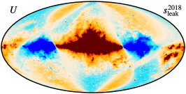
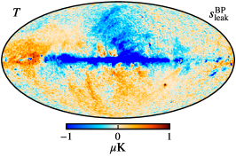
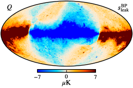
(a) 30 GHz

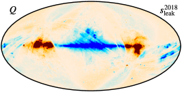
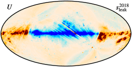
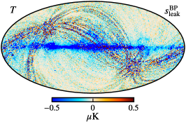
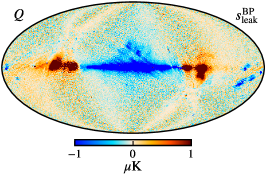
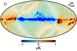
(b) 44 GHz

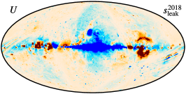
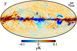
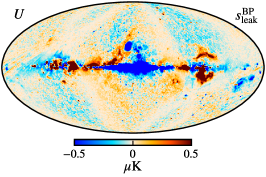
(c) 70 GHz

Figure 9: Full leakage correction maps for the 30 GHz (a), 44 GHz (b) and 70 GHz (c) bands in Stokes $T$, $Q$, and $U$ from the official Planck 2018 processing (top) and BeyondPlanck (bottom). All maps have been smoothed to an angular resolution of 1^∘ FWHM.

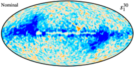
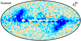
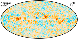
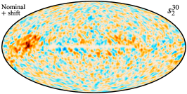
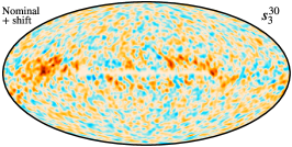
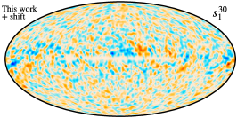
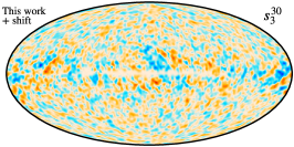
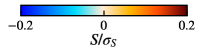
Figure 10: Spurious maps for the 30 GHz band with nominal profiles without corrections (top), nominal profiles with corrections (middle) and new profiles with corrections (bottom) using the processing mask showed in Fig. 5 ($f_{\mathrm{sky}}=0.953$), and smoothed with a gaussian beam of 3^∘ FWHM. This quantity is unitless, as it is defined as $S/\sigma_{S}$.

4.1 Posterior summary

We are now finally ready to present the results from the above algorithms as applied within the BeyondPlanck analysis framework, and we start by inspecting the resulting Markov chains and their internal correlations. As described by BeyondPlanck (2022), two independent Monte Carlo chains are produced in the main BeyondPlanck processing, each resulting in 750 samples. Figure 6 shows a representative subset of these, where in addition to the individual detector bandpass shifts, we also include the AME $\nu_{p}$ parameter in temperature, as well as the spectral index in polarization for both thermal dust and synchrotron, $\beta_{d}$ and $\beta_{s}$, respectively. We note that only the two sampled sky-regions of the synchrotron index are included and not those that are drawn from a prior distribution, see Svalheim et al. (2022) for a full overview.

Overall, we see that the correlation length is substantial in these chains, and it is clear that several of the Metropolis step lengths would benefit from further optimization in a future run. Indeed, using the current chains to tune a Metropolis proposal matrix for a future iteration of the analysis appears to be promising. However, there is in general no doubt that bandpass corrections are among the most difficult parameters to sample in the entire BeyondPlanck data model, because bandpass corrections are global, and do not only affect leakage corrections, but also unit conversions, and thereby the entire foreground model. This global impact leads to a long Markov chain correlation length.

In Fig. 7, we plot Pearson’s correlation coefficient, $p$, for various parameter pairs. Overall, we see that the bandpass parameters are most strongly correlated with the AME peak frequency, $\nu_{\mathrm{p}}$ in intensity, and the synchrotron and thermal dust spectral indices, $\beta_{\mathrm{s}}$ and $\beta_{\mathrm{d}}$, in polarization, for which correlations around $|p|\approx 0.5$ are observed. An in-depth discussion on temperature foreground degeneracies can be found in Andersen et al. (2022). We also note that this plot serves as a powerful reminder of the usefulness of global cross-experiment analysis, as improved constraints on either $\nu_{\mathrm{p}}$, $\beta_{\mathrm{s}}$ or $\beta_{\mathrm{d}}$ from for instance Planck HFI (Planck Collaboration III 2020), C-BASS (King et al. 2010) or QUIJOTE (Génova-Santos et al. 2015) will translate directly into improved constraints on the Planck LFI bandpasses, and therefore better maps overall. Generally speaking, older data sets may almost always be improved when new experiments become available.

The average properties of the Markov chains are listed in Table 4, with the posterior mean and standard deviation for each bandpass correction parameter, both for co-added frequency channels and individual radiometers, and the same information is visualized in Fig. 8.

Figure 9 compares the BeyondPlanck posterior mean leakage maps with the corresponding Planck 2018 LFI leakage maps for all three LFI channels. As discussed in Sect. 3.1, there are several algorithmic differences between these two pipelines. Firstly, the Planck 2018 approach does not account for beam mismatch leakage, and, thus, we see much less small-scale fluctuations in these maps compared to BeyondPlanck; this is particularly striking in the 44 GHz channel. Secondly, we note that the Planck 2018 correction maps exhibit significantly weaker large-scale corrections at high Galactic latitudes compared to BeyondPlanck. We have traced this effect down to a difference in the net foreground monopole in the two approaches, and, in particular, we have found that the BeyondPlanck 30 GHz leakage map takes a very similar shape if we add an artificial negative monopole of $-200\thinspace\mu$K to the AME amplitude map. In this respect, we note that the Planck 2018 pipeline uses the Madam map-making code (Keihänen et al. 2005), which explicitly removes all monopole terms from the co-added map (Planck Collaboration II 2020). At the same time, the Commander-based foreground maps used to generate the correction templates do include a physical estimate of the monopoles. To account for this issue, the DPC processing generated a new set of correction maps using the Planck levelS simulation package (Reinecke et al. 2006), creating TODs from the Commander leakage map and correction factors, and binned these into maps using the same Madam map-making code, resulting in correction maps without the monopole term, from which the final correction templates were generated. In retrospect, it appears that this rather involved pipeline did underestimate the monopole contribution in the final maps, and this serves as a useful reminder of an important benefit of an integrated end-to-end pipeline: Passing data objects from one operation to the next in a self-consistent manner becomes much more transparent when all parts of the code use the same data model.

4.2 Comparison of nominal and corrected LFI bandpasses

Figure 11: Estimated bandpass corrections for the 70 GHz radiometer. Estimated bandpass corrections for each LFI radiometer. These parameters are constrained to have vanishing mean, and are as such strongly correlated.

As discussed in Sect. 2, we have applied a number of pre-processing steps to the Planck LFI bandpasses before performing the main BeyondPlanck end-to-end analysis. In this section, we consider the impact of these changes in terms of some key data products that highlight their effects.

The first quantity we consider is the spurious map, $S_{j}$, as defined by Eq. (16). These are shown for the 30 GHz channel in Fig. 10 for three different analysis configurations, all in the form of $S_{j}/\sigma_{j}$, masked by the bandpass processing mask, and smoothed to $3^{\circ}$ FWHM. The top row shows the three 30 GHz spurious maps that result if one attempts to produce maps with no bandpass corrections at all, and simply takes the publicly available profiles at face value. Here we see coherent structures that are clearly inconsistent with noise, and morphologically associated with the Galactic plane and the so-called “Planck Deep Fields” (centered on the Ecliptic poles). In these regions, the $S$ signal-to-noise ratio is vastly higher than in the Ecliptic plane, because of the dense polarization angle sampling of the Planck scanning strategy. The second row shows a similar case, using the nominal LFI bandpasses, but this time allowing a frequency shift per radiometer, as described in Sect. 3. The residuals are clearly reduced, indicating that the fitting algorithm does work as expected. Finally, the bottom row shows the same, but now using the corrected LFI bandpasses from Sect. 2 as input. At this point, the residuals are significantly closer to randomly distributed, with only small residuals appearing near the Galactic center.

Figure 11 shows a comparison of posterior mean and standard deviations for the 70 GHz bandpass corrections when using the nominal (orange points) and corrected (blue points) profiles. Here, we see that the nominal profiles generally require much larger correction factors than the corrected profiles. In particular, 18M sees $\Delta_{\mathrm{bp}}\sim 1.3$ GHz using the nominal profiles as opposed to $\sim 0.8\thinspace$GHz for the new. This is not surprising, considering that this profile exhibits some of the strongest systematic artefacts in Fig. 1.

5 Conclusions

In this paper, we have discussed how bandpass and beam leakage effects may be mitigated in a Bayesian CMB analysis pipeline, and summarized the results from the BeyondPlanck pipeline. As a preparatory step, we have also provided a set of corrected LFI bandpass profiles that correct for known systematic features dating back to the ground calibration phase and previously reported in the literature. The most notable result from these corrections is that the overall 70 GHz center frequency is shifted up by 0.6 %, and simple map-based comparisons show that differences in the resulting frequency maps are on the order of a couple of microkelvins.

We argue that the proposed algorithms are substantially simpler to implement compared to previous methods, due to the tight integration between astrophysical component separation and low-level mapmaking; all the required components are already available from different parts of the BeyondPlanck framework. As a result, the leakage correction may actually be defined in terms of two or three very simple equations, and the practical code implementation amounts to a few hundred lines of code. We also note that beam leakage corrections are trivial to implement, simply by accounting for the different detector beam responses when scanning the model sky with the pointing operator.

We believe that the importance of these methods will become increasingly critical for next-generation experiments. While the current Planck LFI polarization observations are intrinsically noise dominated, and the various corrections discussed in this paper are relatively minor compared to the overall noise level, the same will not hold true for future $B$-mode experiments such as LiteBIRD or CMB-S4; for these, establishing highly accurate bandpass and beam leakage corrections will be absolutely essential in order to reach the required nanokelvin accuracy.