Equivalence Between Four Models of Associahedra

Abstract.

We present a combinatorial isomorphism between Stasheff associahedra and an inductive cone construction of those complexes given by Loday. We give an alternate description of certain polytopes, known as multiplihedra, which arise in the study of $A_{\infty}$ maps. We also provide new combinatorial isomorphisms between Stasheff associahedra, collapsed multiplihedra, and graph cubeahedra for path graphs.

1. Introduction

Dov Tamari, in his 1951 thesis [32], first described associahedra (with notation $\mathscr{M}_{n-1}$) as the realization of his poset lattice of bracketings (parenthesizations) of a word with $n$ letters. He had also pictured the $1$, $2$ and $3$ dimensional cases (cf. figure 1(a)). Later these were rediscovered by Jim Stasheff [29] in his 1960 thesis on homotopy associativity and based loop spaces. Stasheff had defined these (with notation $K_{n}$) as a convex, curvilinear subset of the $(n-2)$ dimensional unit cube (cf. figure 1(b)) such that it is homeomorphic to the cube. Convex polytope realization of associahedra were subsequently done by many people [16, 15, 19, 20]. These polytopes are commonly known as associahedra or Stasheff polytopes.
     Ever since Stasheff’s work, associahedra (and their face complexes) have continued to appear in various mathematical fields apart from its crucial role in homotopy associative algebras and its important role in discrete geometry. Indeed, the associahedron $K_{n-1}$ appears as a fundamental tile of $\overline{\mathcal{M}}_{0,n}(\mathbb{R})$, the compactification of the real moduli space of punctured Riemann sphere [7]. It also appears in the analysis of the compactified moduli space of nodal disks with markings, as described by Fukaya and Oh [14]. An important connection between associahedra (and its generalizations) and finite root systems was established in 2003 by the work of Fomin and Zelevinsky [10]. In 2006 Carr and Devadoss [5] generalized associahedra to graph associahedra $\mathcal{K}G$ for a given graph $G$. These appear as the tiling of minimal blow-ups of certain Coxeter complexes [5]. In particular, if $G$ is a path graph, then $\mathcal{K}G$ is an associahedron. Bowlin and Brin [4], in 2013, gave a precise conjecture about existence of coloured paths in associahedra. They showed that this conjecture is equivalent to the four colour theorem (4CT). Earlier, in 1988, there was a celebrated work [27] of Sleator, Tarjan and Thurston on the diameter of associahedra. While working on dynamic optimality conjecture, they had used hyperbolic geometry techniques to show that the diameter of $K_{d}$ is at most $2d-8$ when $d\geq 11$, and this bound is sharp when $d$ is large enough. Pournin [25], almost twenty five years later, showed that this bound is sharp for $d\geq 11$. Moreover, his proof was combinatorial. Even in theoretical physics, recent works [24, 2, 9] indicate that associahedron plays a key role in the theory of scattering amplitudes.

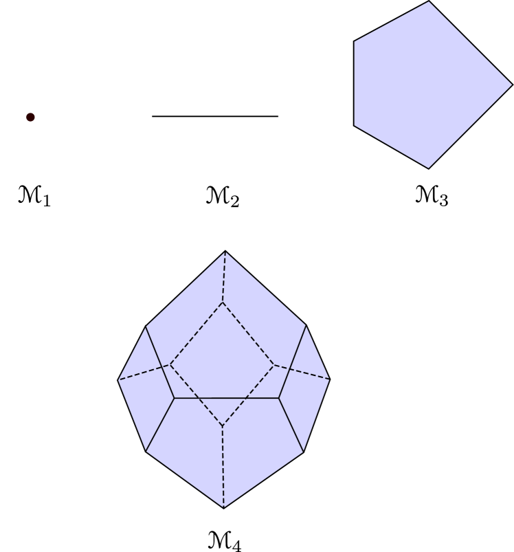
(a) Tamari’s associahedra

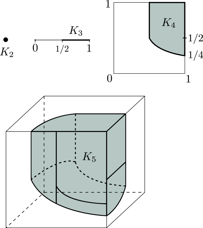
(b) Stasheff’s associahedra

Figure 1. Earliest realizations of associahedra

Let us briefly recall the construction in [29]. Stasheff, respecting Tamari’s description, had sub-divided the boundary of $K_{n}$ in such a way that the number of faces of codimension $1$ and the adjacencies in his model matched with that in [32]. The boundary of $K_{n}$, denoted by $L_{n}$, is the union of homeomorphic images of $K_{p}\times_{r}K_{q}$ ($p+q=n+1$, $r=1,2,...,p$), where $K_{p}\times_{r}K_{q}$ corresponds to the bracketing $x_{1}\ldots(x_{r}\ldots x_{r+q-1})\ldots x_{n}$. Stasheff started with $K_{2}$ as a point and defined $K_{n}$, inductively, as a cone over $L_{n}$. This definition of $K_{n}$ involves $K_{2}$ through $K_{n-1}$ all together.
     As associahedra are contractible, these are of less interest as spaces in isolation. However, as combinatorial objects, the key properties of it are inherent in its description as a convex polytope. Much later, in 2005, J. L. Loday [21] gave a different inductive construction of $K_{n}$ starting from $K_{n-1}$, leaving it to the reader to verify the details. Being a predominantly topological construction, it is not apparent why the cone construction of Loday gives rise to the known combinatorial structure on the associahedra. It is, therefore, natural to search for an explicit combinatorial isomorphism between these two constructions, leading to our first result (Theorem 3.2).

Theorem A.

Stasheff polytopes are combinatorially isomorphic to Loday’s cone construction of associahedra.

There is another set of complexes $\mathcal{J}(n)$, known as multiplihedra, which were first introduced and pictured by Stasheff [28] in order to define $A_{\infty}$ maps between $A_{\infty}$ spaces, for $n\leq 4$. Mau and Woodward [22] have shown $\mathcal{J}(n)$’s to be compactification of the moduli space of quilted disks. Boardman and Vogt [3] provided a definition of $\mathcal{J}(n)$ in terms of painted trees (refer to Definition 2.8). The first detailed definition of $\mathcal{J}(n)$ and its combinatorial properties were described by Iwase and Mimura [17], while its realization as convex polytopes was achieved by Forcey [11], combining the description of Boardman-Vogt and Iwase-Mimura. Later, Devadoss and Forcey [6] generalized multiplihedra to graph multiplihedra $\mathcal{J}G$ for a given graph $G$.

In the study of $A_{\infty}$ maps from an $A_{\infty}$ space to a strictly associative $H$ space (i.e., a topological monoid), multiplihedra degenerate to what we call collapsed multiplihedra. Stasheff [28] had pointed out that these polytopes resemble associahedra. It has been observed that collapsed multiplihedra can be viewed as degeneration of graph multiplihedra for path graphs. It was long assumed that for $A_{\infty}$ maps from a strictly associative $H$ space to a $A_{\infty}$ space, multiplihedra would likewise degenerate to yield associahedra. But it was Forcey [12] who realized that new polytopes were needed. These were constructed by him and named composihedra.
     In this paper, we will give an equivalent definition (Definition 2.12) of multiplihedra, which induces a definition for collapsed multiplihedra (Definition 2.14). Using this definition, we will give a proof of the following (Proposition 3.4) by providing a new bijection of underlying posets.

Observation b.

Stasheff polytopes and collapsed multiplihedra are combinatorially isomorphic.

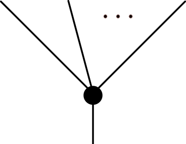
(a)

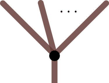
(b)

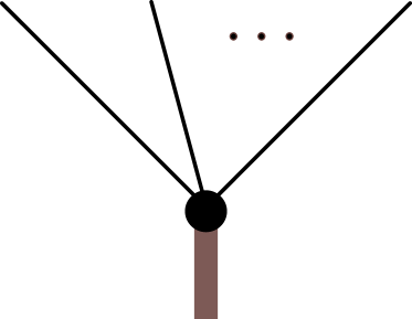
(c)

Figure 7. Admissible nodes

There is a well-known bijection $bij_{3}$ (cf. Forcey’s paper [13, p. 195]; prior to Remark 2.6 and Figure 7) which is different from ours.

In 2010, Devadoss, Heath, and Vipismakul [8] defined a polytope called graph cubeahedron (denoted by $\mathcal{C}G$) associated to a graph $G$. These are obtained by truncating certain faces of a cube. They gave a convex realization of these polytopes as simple convex polytopes whose face poset is isomorphic to the poset of design tubings for graphs. Graph cubeahedra for cycle graphs $G$ (called halohedra) appear as the moduli space of annulus with marked points on one boundary circle. In this paper, we are mainly interested in $\mathcal{C}G$ for path graphs $G$ and will prove the following (Proposition 3.5) by providing a new bijection of underlying posets.

Observation c.

The collapsed multiplihedra and graph cubeahedra for path graphs are combinatorially isomorphic.

It turns out that bijection obtained between the posets governing Stasheff polytopes and graph cubeahedra (for path graphs), by combining our bijections from Observations b and c, is the bijection of posets defined in [8, Proposition 14]. Form our perspective, the bijection in Observation c is natural. Combining Theorem A, Observations b and c, we obtain the following result (Theorem 3.1).

Theorem B.

The four models of associahedra - Stasheff polytopes, complexes obtained by Loday’s cone construction, collapsed multiplihedra, graph cubeahedra for path graphs - are all combinatorially isomorphic.

Organization of the paper. The paper is organized as follows. In §2.1, we will review some of the definitions and results related to Stasheff’s description of associahedra. In §2.2, the description of Loday’s cone construction and some related theorems are presented while in §2.3 an equivalent definition of multiplihedra and collapsed multiplihedra are given. In §2.4 the definition of tubings, design tubings, graph cubeahedra, and related results are presented. The next section §3 contains the proof of the main result (Theorem B), which is a combination of three results. In §3.1 we prove Theorem A while §3.2 and §3.3 are devoted to the proofs of Observations b and c respectively.

Acknowledgments. The authors would like to thank Stefan Forcey for an initial discussion on this topic as well as several useful comments on the first draft. The first author acknowledges the support of SERB MATRICS grant MTR/2017/000807 for the funding opportunity. The second author is supported by a PMRF fellowship.

2. Description of Four Models of Associahedra

An $H$-space is a topological space $X$ equipped with a binary operation $m:X^{2}\to X$ having a unit $e$. It is a natural generalization of the notion of topological groups. We can rewrite $m$ as a map $m_{2}:K_{2}\times X^{2}\to X$, where $K_{2}$ is a point. If $m$ is not associative but homotopy associative (called weakly associative), then we have a map $m_{3}:K_{3}\times X^{3}\to X$ defined through the homotopy between $m\mathbin{\mathchoice{\vbox{\hbox{$\scriptstyle\circ$}}}{\vbox{\hbox{$\scriptstyle\circ$}}}{\vbox{\hbox{$\scriptscriptstyle\circ$}}}{\vbox{\hbox{$\scriptscriptstyle\circ$}}}}(m\times 1)$ and $m\mathbin{\mathchoice{\vbox{\hbox{$\scriptstyle\circ$}}}{\vbox{\hbox{$\scriptstyle\circ$}}}{\vbox{\hbox{$\scriptscriptstyle\circ$}}}{\vbox{\hbox{$\scriptscriptstyle\circ$}}}}(1\times m)$, where $K_{3}$ is an interval. Similarly, we can define five different maps from $X^{4}\to X$ using $m$, and between any two such maps, there are two different homotopies (using the chosen homotopy associativity). If those two homotopies are homotopic themselves, then this defines a map $m_{4}:K_{4}\times X^{4}\to X$, where $K_{4}$ is a filled pentagon. If we continue this process, we obtain a map $m_{n}:K_{n}\times X^{n}\to X$ for $n\geq 2$. These complexes $K_{n}$, called associahedra, are our main objects of interest.

We will briefly describe the four models of associahedra, one in each subsection, we are concerned with: Stasheff polytopes, Loday’s cone construction, collapsed multiplihedra, and graph cubeahedra for path graphs.

2.1. Stasheff Polytopes

Stasheff defined for each $i\geq 2$, a special cell complex $K_{i}$ as a subset of $I^{i-2}$. It is a simplicial complex and has $i$ degeneracy operators $s_{1},...,s_{i}$. Moreover, $K_{i}$ has $\binom{i}{2}-1$ faces of codimension $1$. The complexes $K_{i}$, as combinatorial objects, are more complicated than the standard simplices $\Delta^{i-2}$. According to Stasheff [29], it is defined through following intuitive content:
Consider a word with $i$ letters and all meaningful ways of inserting one set of parentheses. To each such insertion except for $(x_{1},x_{2},...,x_{i})$, there corresponds a cell of $L_{i}$, the boundary of $K_{i}$. If the parentheses enclose $x_{k}$ through $x_{k+s-1}$, we regard this cell as $K_{r}\times_{k}K_{s}$, the homeomorphic image of $K_{r}\times K_{s}$ under a map which we call $\partial_{k}(r,s)$, where $r+s=i+1$. Two such cells intersect only on their boundaries and the ‘edges’ so formed correspond to inserting two sets of parentheses in the word. Thus we have the relations:

• $\partial_{j}(r,s+t-1)\left(1\times\partial_{k}(s,t)\right)=\partial_{j+k-1}(r+s-1,t)\left(\partial_{j}(r,s)\times 1\right)$

• $\partial_{j+s-1}(r+s-1,t)\left(\partial_{k}(r,s)\times 1\right)=\partial_{k}(r+t-1,s)\left(\partial_{j}(r,t)\times 1\right)(1\times T)$

where $T:K_{s}\times K_{t}\rightarrow K_{t}\times K_{s}$ permutes the factors. Observe that, in terms of homeomorphic images of $K_{r}\times K_{s}\times K_{t}$, the two relations above are equivalent respectively to the identifications

$$K_{r}\times_{j}(K_{s}\times_{k}K_{t})=(K_{r}\times_{j}K_{s})\times_{j+k-1}K_{t}$$ (1)

$$(K_{r}\times_{k}K_{s})\times_{j+s-1}K_{t}=(K_{r}\times_{j}K_{t})\times_{k}K_{s}$$ (2)

This is enough to obtain $K_{i}$ by induction. Start with $K_{2}=\{\ast\}$ as a point. Given $K_{2}$ through $K_{i-1}$, construct $L_{i}$ by fitting together copies of $K_{r}\times_{k}K_{s}$ as indicated by the above conditions. Take $K_{i}$ to be the cone on $L_{i}$. Stasheff proved that these polytopes are homeomorphic to cubes.

Proposition 2.1.

[29, Proposition 3] $K_{i}$ is homeomorphic to $I^{i-2}$ and degeneracy maps $s_{j}:K_{i}\rightarrow K_{i-1}$ for $1\leq j\leq i$ can be defined so that the following relations hold:

1. $s_{j}s_{k}=s_{k}s_{j+1}$ for $k\leq j$.

2. $s_{j}\partial_{k}(r,s)=\partial_{k-1}(r-1,s)\left(s_{j}\times 1\right)$ for $j<k$ and $r>2$.

3. $s_{j}\partial_{k}(r,s)=\partial_{k}(r,s-1)\left(1\times s_{j-k+1}\right)$ for $s>2,k\leq j<k+s,\\ s_{j}\partial_{k}(i-1,2)=\pi_{1}$ for $1<j=k<i$ and $1<j=k+1\leq i,$
   $s_{1}\partial_{2}(2,i-1)=\pi_{2}$ and $s_{i}\partial_{1}(2,i-1)=\pi_{2}$,
   where $\pi_{m}$ for $m=1,2$ is projection onto the $m$th factor.

4. $s_{j}\partial_{k}(r,s)=\partial_{k}(r-1,s)\left(s_{j-s+1}\times 1\right)$ for $k+s\leq j$.

Using boundary maps $\partial_{k}(r,s)$ and degeneracy maps $s_{j}$, Stasheff defined the following.

Definition 2.2 ($A_{n}$ form and $A_{n}$ space).

An $A_{n}$ form on a space $X$ consists of a family of maps $m_{i}:K_{i}\times X^{i}\to X$ for $2\leq i\leq n$ such that

1. there exists $e\in X$ with $m_{2}(*,e,x)=m_{2}(*,x,e)=x$ for $x\in X,*=K_{2}$.

2. For $\rho\in K_{r},\sigma\in K_{s},r+s=i+1$, we have

   $$m_{i}\left(\partial_{k}(r,s)(\rho,\sigma),x_{1},\cdots,x_{i}\right)=m_{r}\left(\rho,x_{1},\cdots,x_{k-1},m_{s}\left(\sigma,x_{k},\cdots,x_{k+s-1}\right),x_{k+s},\cdots,x_{i}\right).$$

3. For $\tau\in K_{i}$ and $i>2$, we have

   $$m_{i}\left(\tau,x_{1},\cdots,x_{j-1},e,x_{j+1},\cdots,x_{i}\right)=m_{i-1}\left(s_{j}(\tau),x_{1},\cdots,x_{j-1},x_{j+1},\cdots,x_{i}\right).$$

The pair $(X,\{m_{i}\}_{2\leq i\leq n})$ is called an $A_{n}$ space.
If the maps $m_{i}$ exist for all $i$, then it is called an $A_{\infty}$ form and the corresponding pair is called an $A_{\infty}$ space.

Homotopy associative algebras (or $A_{\infty}$ algebras), $A_{\infty}$ spaces and operads have been extensively studied. The interested reader is directed to the excellent books [23, 3, 1] and introductory notes [18]. Related to the notion of $A_{n}$ space, Stasheff [29] also defined the notion of $A_{n}$ structure.

Definition 2.3 ($A_{n}$ structure).

An $A_{n}$ structure on a space $X$ consists of an $n$-tuple of maps $p_{i}:E_{i}\to B_{i}$ for $1\leq i\leq n$ with $X=E_{1}\subset E_{2}\subset\cdots\subset E_{n}$ and $*=B_{1}\subset B_{2}\subset\cdots B_{n}$ such that $p_{i*}:\pi_{q}(E_{i},X)\to\pi_{q}(B_{i})$ is an isomorphism for all $q$, together with a contracting homotopy $h:CE_{n-1}\to E_{n}$ such that $h(CE_{i-1})\subset E_{i}$.

One of the key results in Stasheff [29, Theorem 5] states that a space admits $A_{n}$ structure if and only if it has an $A_{n}$ form. Topological groups and more generally based loop spaces admit $A_{n}$ structures for all values of $n$. The landmark result in [29, Remarks before §6 in page 283 of HAH-I], essentially motivated by earlier works of Sugawara [31, Theorem 4.2], [30, Lemma 10], is a recognition principle for based loop spaces.

Theorem 2.4 (Stasheff).

A space $Y$, having the homotopy type of a CW complex, is an $A_{\infty}$ space if and only if $Y$ is homotopy equivalent to a based loop space.

In this paper, however, we are exclusively interested in the combinatorial description of the complexes $K_{i}$. The correspondence between faces of Stasheff polytopes (associahedra) and the bracketings indicate that these polytopes can also be defined as follows.

Definition 2.5 (Associahedron).

Let $\mathfrak{P}(n)$ be the poset of bracketings of a word with $n$ letters, ordered such that $p<p^{\prime}$ if $p$ is obtained from $p^{\prime}$ by adding new brackets. The associahedron $K_{n}$ is a convex polytope of dimension $n-2$ whose face poset is isomorphic to $\mathfrak{P}(n)$.

This construction of the polytope $K_{n}$ was first given in 1984 by Haiman in his (unpublished) manuscript [15]. In 1989, C. Lee [19, Theorem 1] proved this by considering the collection of all sets of mutually non-crossing diagonals of a polygon. Observe that the sets of mutually non-crossing diagonals of an $(n+1)$-gon are in bijective correspondence with the bracketings of a word with $n$ letters. We will use this description later in §3.2.

2.2. Loday’s Cone Construction

From the combinatorial description given by Stasheff, the associahedron $K_{n}$ is a polytope of dimension $n-2$ whose vertices are in bijective correspondence with the $(n-2)$-bracketing of the word $x_{1}x_{2}\ldots x_{n}$. But each $(n-2)$-bracketing of the word $x_{1}x_{2}\ldots x_{n}$ corresponds to a rooted planar binary tree with $n+1$ leaves, one of them being the root. For example, the planar rooted trees associated to $x_{1}(x_{2}(x_{3}x_{4}))$ and $(x_{1}x_{2})(x_{3}x_{4})$ are depicted below (cf. figure 2(a), 2(b)), the root being represented by the vertical leaf in each case.

for tree=minimum width = 4em, delay = where content=shape=coordinate, calign=fixed edge angles, calign angle=45, grow=north, , text centered, [[[[[][,tier=L]][,tier=L]][,tier=L]]]

(a) $x_{1}(x_{2}(x_{3}x_{4}))$

for tree=minimum width = 4em, delay = where content=shape=coordinate, calign=fixed edge angles, calign angle=45, grow=north, , text centered, [[[[][,tier=L]][ ,phantom,fit=band][[][,tier=L]]]]

(b) $(x_{1}x_{2})(x_{3}x_{4})$

Figure 2. Correspondence between bracketing and rooted binary tree

Thus $K_{n}$ can also be thought of as a polytope of dimension $n-2$ whose vertices are in bijective correspondence with planar rooted binary trees with $n$ leaves and $1$ root. Let $Y_{n}$ be the set of such trees. The trees are depicted below for $2\leq n\leq 4$.

$$Y_{2}=\left\{\begin{matrix}\scalebox{0.3}{ \forest for tree={minimum width = 4em, delay = {where content={}{shape=coordinate}{}, calign=fixed edge angles, calign angle=45, grow=north, }, text centered, } [[[][]]] }\end{matrix}\right\},\ Y_{3}=\left\{\begin{matrix}\scalebox{0.2}{ \forest for tree={minimum width = 4em, delay = {where content={}{shape=coordinate}{}, calign=fixed edge angles, calign angle=45, grow=north, }, text centered, } [[[[][,tier=L]][,tier=L]]] },\scalebox{0.2}{ \forest for tree={minimum width = 4em, delay = {where content={}{shape=coordinate}{}, calign=fixed edge angles, calign angle=45, grow=north, }, text centered, } [[[,tier=L][[,tier=L][]]]] }\end{matrix}\right\},\ Y_{4}=\left\{\begin{matrix}\scalebox{0.15}{ \forest for tree={minimum width = 4em, delay = {where content={}{shape=coordinate}{}, calign=fixed edge angles, calign angle=45, grow=north, }, text centered, } [[[,tier=L][[,tier=L][[,tier=L][]]]]] },\scalebox{0.2}{ \forest for tree={minimum width = 4em, delay = {where content={}{shape=coordinate}{}, calign=fixed edge angles, calign angle=45, grow=north, }, text centered, } [[[[][]][[][]]]] },\scalebox{0.15}{ \forest for tree={minimum width = 4em, delay = {where content={}{shape=coordinate}{}, calign=fixed edge angles, calign angle=45, grow=north, }, text centered, } [[[,tier=L][[[][,tier=L]][,tier=L]]]] },\scalebox{0.15}{ \forest for tree={minimum width = 4em, delay = {where content={}{shape=coordinate}{}, calign=fixed edge angles, calign angle=45, grow=north, }, text centered, } [[[[,tier=L][[,tier=L][,tier=L]]][,tier=L]]] },\scalebox{0.15}{ \forest for tree={minimum width = 4em, delay = {where content={}{shape=coordinate}{}, calign=fixed edge angles, calign angle=45, grow=north, }, text centered, } [[[[[][,tier=L]][,tier=L]][,tier=L]]] }\end{matrix}\right\}$$

Any $t\in Y_{n}$ is defined to have degree $n$. We label the leaves (not the root) of $t$ from left to right by $0,1,\cdots,n-1$. Then we label the internal vertices by $1,2,\cdots,n-1$. The $i$th internal vertex is the one which falls in between the leaves $i-1$ and $i$. We denote by $a_{i}$, respectively $b_{i}$, the number of leaves on the left side, respectively right side, of the $i$th vertex. The product $a_{i}b_{i}$ is called the weight of the $i$th internal vertex. To each tree $t\in Y_{n}$, we associate the point $M(t)\in\mathbb{R}^{n-1}$, whose $i$th coordinate is the weight of the $i$th vertex:

$$M(t)=\left(a_{1}b_{1},\cdots,a_{i}b_{i},\cdots,a_{n-1}b_{n-1}\right)\in\mathbb{R}^{n-1}$$

For instance,

$$M\left(\begin{matrix}\scalebox{0.2}{ \forest for tree={minimum width = 4em, delay = {where content={}{shape=coordinate}{}, calign=fixed edge angles, calign angle=45, grow=north, }, text centered, } [[[][]]] }\end{matrix}\right)=(1),\ M\left(\begin{matrix}\scalebox{0.18}{ \forest for tree={minimum width = 4em, delay = {where content={}{shape=coordinate}{}, calign=fixed edge angles, calign angle=45, grow=north, }, text centered, } [[[[][,tier=L]][,tier=L]]] }\end{matrix}\right)=(2,1),\ M\left(\begin{matrix}\scalebox{0.18}{ \forest for tree={minimum width = 4em, delay = {where content={}{shape=coordinate}{}, calign=fixed edge angles, calign angle=45, grow=north, }, text centered, } [[[,tier=L][[,tier=L][]]]] }\end{matrix}\right)=(1,2),$$

$$M\left(\begin{matrix}\scalebox{0.13}{ \forest for tree={minimum width = 4em, delay = {where content={}{shape=coordinate}{}, calign=fixed edge angles, calign angle=45, grow=north, }, text centered, } [[[,tier=L][[,tier=L][[,tier=L][]]]]] }\end{matrix}\right)=(1,2,3),\ M\left(\begin{matrix}\scalebox{0.18}{ \forest for tree={minimum width = 4em, delay = {where content={}{shape=coordinate}{}, calign=fixed edge angles, calign angle=45, grow=north, }, text centered, } [[[[][]][[][]]]] }\end{matrix}\right)=(1,4,1)$$

Observe that the weight of a vertex depends only on the sub-tree that it determines. Using these integral coordinates, Loday [20] gave a convex realization of $K_{n+1}$ in $\mathbb{R}^{n}$.

Lemma 2.6.

[20, Lemma 2.5] For any tree $t\in Y_{n+1}$ the coordinates of the point $M(t)=\left(x_{1},\cdots,x_{n}\right)\in\mathbb{R}^{n}$ satisfy the relation

$$\sum_{k=1}^{n}x_{k}=\textstyle{\frac{1}{2}n(n+1)}.$$

Thus, it follows that

$$M(t)\in H_{n}=\left\{(x_{1},...,x_{n})\in\mathbb{R}^{n}:x_{1}+x_{2}+...+x_{n}=\textstyle{\frac{n(n+1)}{2}}\right\}.$$

Theorem 2.7.

[20, Theorem 1.1] The convex hull of the points $M(t)\in\mathbb{R}^{n}$, for $t\in Y_{n+1}$, is a realization of the Stasheff polytope $K_{n+1}$ of dimension $n-1$.

For example, the polytope $K_{5}$ lies in the hyperplane $H_{4}$ in $\mathbb{R}^{4}$. Under an isometric transformation of $H_{4}$ to $\mathbb{R}^{3}$ (i.e., $x_{4}=0$ hyperplane), the embedded picture of $K_{5}$ is shown in figure 3.

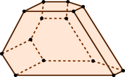
Figure 3. Loday’s embedded $K_{5}$ in $\mathbb{R}^{3}$

Now starting with $K_{2}$ as point, Loday [21, §2.4] gave a different inductive construction of the polytopes $K_{n+1}$. The steps are as follows:

1. Start with the associahedron $K_{n}$, which is a ball and whose boundary is a cellular sphere. The cells of the boundary are of the form $K_{p}\times_{r}K_{q}$ where $p+q=n+1$ and $r=1,2,...,p$.

2. Enlarge each cell $K_{p}\times_{r}K_{q}$ into a cell of dimension $n$ by replacing it by $K_{p+1}\times_{r}K_{q}$. We denote the total enlarged complex by $\widehat{K}_{n}$.

3. Take the cone over the above enlargement and declare that to be $K_{n+1}$, i.e. $K_{n+1}:=C(\widehat{K}_{n})$.

The following examples in low dimensions illustrate how this process works.

• To construct $K_{3}$ from $K_{2}$, form the enlarged complex $\widehat{K}_{2}$, which is a point (as $K_{2}$ has no boundary). Then $K_{3}$ is cone over the point $\widehat{K}_{2}$, i.e., an interval.
  

  

  Figure 4. $K_{3}$ from $K_{2}$

• To construct $K_{4}$ from $K_{3}$, note that $K_{3}$ has two boundary points namely $K_{2}\times_{1}K_{2}$ and $K_{2}\times_{2}K_{2}$. Thus $\widehat{K}_{3}$ consist of the original $K_{3}$ together with $K_{3}\times_{1}K_{2}$ and $K_{3}\times_{2}K_{2}$, which looks like an angular ‘C’ shape. Finally $K_{4}$ is the cone over $\widehat{K}_{3}$, resulting in a filled pentagon.
  

  

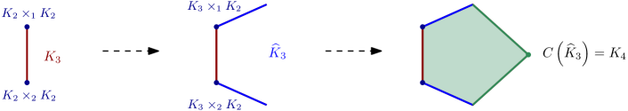
  Figure 5. $K_{4}$ from $K_{3}$

2.3. Collapsed Multiplihedra

Suppose $(X\{m_{i}\}),(Y,\{m_{i}^{\prime}\})$ are two $A_{\infty}$ spaces and $f:X\to Y$ is a weak homomorphism i.e., there is a homotopy between the maps $f\mathbin{\mathchoice{\vbox{\hbox{$\scriptstyle\circ$}}}{\vbox{\hbox{$\scriptstyle\circ$}}}{\vbox{\hbox{$\scriptscriptstyle\circ$}}}{\vbox{\hbox{$\scriptscriptstyle\circ$}}}}m_{2}$ and $m_{2}^{\prime}\mathbin{\mathchoice{\vbox{\hbox{$\scriptstyle\circ$}}}{\vbox{\hbox{$\scriptstyle\circ$}}}{\vbox{\hbox{$\scriptscriptstyle\circ$}}}{\vbox{\hbox{$\scriptscriptstyle\circ$}}}}(f\times f)$. Such maps called $H$-maps. In general, there is a notion of $A_{n}$ maps in Stasheff [29, II, Def. 4.1], which satisfy $f\mathbin{\mathchoice{\vbox{\hbox{$\scriptstyle\circ$}}}{\vbox{\hbox{$\scriptstyle\circ$}}}{\vbox{\hbox{$\scriptscriptstyle\circ$}}}{\vbox{\hbox{$\scriptscriptstyle\circ$}}}}m_{i}=m_{i}^{\prime}\mathbin{\mathchoice{\vbox{\hbox{$\scriptstyle\circ$}}}{\vbox{\hbox{$\scriptstyle\circ$}}}{\vbox{\hbox{$\scriptscriptstyle\circ$}}}{\vbox{\hbox{$\scriptscriptstyle\circ$}}}}(1\times f^{i})$ for $i\leq n$. Thus we have a map $f_{2}:\mathcal{J}(2)\times X^{2}\to Y$, where $\mathcal{J}(2)$ is an interval. To match things up, rewrite $f$ as $f_{1}:\mathcal{J}(1)\times X\to Y$, where $\mathcal{J}(1)$ is a single point. Now using $m_{2},m_{2}^{\prime},f$, there are six different ways (cf. figure 8) to define a map from $X^{3}$ to $Y$, namely $f\mathbin{\mathchoice{\vbox{\hbox{$\scriptstyle\circ$}}}{\vbox{\hbox{$\scriptstyle\circ$}}}{\vbox{\hbox{$\scriptscriptstyle\circ$}}}{\vbox{\hbox{$\scriptscriptstyle\circ$}}}}(m_{2}\mathbin{\mathchoice{\vbox{\hbox{$\scriptstyle\circ$}}}{\vbox{\hbox{$\scriptstyle\circ$}}}{\vbox{\hbox{$\scriptscriptstyle\circ$}}}{\vbox{\hbox{$\scriptscriptstyle\circ$}}}}(m_{2}\times 1)),$ $f\mathbin{\mathchoice{\vbox{\hbox{$\scriptstyle\circ$}}}{\vbox{\hbox{$\scriptstyle\circ$}}}{\vbox{\hbox{$\scriptscriptstyle\circ$}}}{\vbox{\hbox{$\scriptscriptstyle\circ$}}}}(m_{2}\mathbin{\mathchoice{\vbox{\hbox{$\scriptstyle\circ$}}}{\vbox{\hbox{$\scriptstyle\circ$}}}{\vbox{\hbox{$\scriptscriptstyle\circ$}}}{\vbox{\hbox{$\scriptscriptstyle\circ$}}}}(1\times m_{2})),$ $m_{2}^{\prime}\mathbin{\mathchoice{\vbox{\hbox{$\scriptstyle\circ$}}}{\vbox{\hbox{$\scriptstyle\circ$}}}{\vbox{\hbox{$\scriptscriptstyle\circ$}}}{\vbox{\hbox{$\scriptscriptstyle\circ$}}}}(f\times m_{2}),$ $m_{2}^{\prime}\mathbin{\mathchoice{\vbox{\hbox{$\scriptstyle\circ$}}}{\vbox{\hbox{$\scriptstyle\circ$}}}{\vbox{\hbox{$\scriptscriptstyle\circ$}}}{\vbox{\hbox{$\scriptscriptstyle\circ$}}}}(m_{2}\times f),$ $m_{2}^{\prime}\mathbin{\mathchoice{\vbox{\hbox{$\scriptstyle\circ$}}}{\vbox{\hbox{$\scriptstyle\circ$}}}{\vbox{\hbox{$\scriptscriptstyle\circ$}}}{\vbox{\hbox{$\scriptscriptstyle\circ$}}}}(1\times m_{2}^{\prime})\mathbin{\mathchoice{\vbox{\hbox{$\scriptstyle\circ$}}}{\vbox{\hbox{$\scriptstyle\circ$}}}{\vbox{\hbox{$\scriptscriptstyle\circ$}}}{\vbox{\hbox{$\scriptscriptstyle\circ$}}}}(f\times f\times f),$ $m_{2}^{\prime}\mathbin{\mathchoice{\vbox{\hbox{$\scriptstyle\circ$}}}{\vbox{\hbox{$\scriptstyle\circ$}}}{\vbox{\hbox{$\scriptscriptstyle\circ$}}}{\vbox{\hbox{$\scriptscriptstyle\circ$}}}}(m_{2}^{\prime}\times 1)\mathbin{\mathchoice{\vbox{\hbox{$\scriptstyle\circ$}}}{\vbox{\hbox{$\scriptstyle\circ$}}}{\vbox{\hbox{$\scriptscriptstyle\circ$}}}{\vbox{\hbox{$\scriptscriptstyle\circ$}}}}(f\times f\times f)$. Using the weak homomorphism of $f$ and weak associativity in $X,Y$ (due to the existence of $m_{3}$, $m_{3}^{\prime}$), one realizes that there are two different homotopies between any two of the six maps. If those two homotopies are homotopic themselves, then we have a map $f_{3}:\mathcal{J}(3)\times X^{3}\to Y$, where $\mathcal{J}(3)$ is a filled hexagon.

If we continue this process, we will get a map $f_{n}:\mathcal{J}(n)\times X^{n}\to Y$ for each $n\geq 1$. These complexes $\mathcal{J}(n)$ are called multiplihedra. In the figure 6(b) below, the blue edges collapses to a point so that the rectangular faces degenerate to brown edges and the pentagonal face degenerates to a single point, giving rise to Loday’s realization of $K_{5}$. There is a different degeneration from $\mathcal{J}(n)$ to $K_{n+1}$, as shown in [26, §5]; figure 6(c) exhibits this for $\mathcal{J}(4)$.

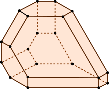
(a) Embedded $\mathcal{J}(4)$ in $\mathbb{R}^{3}$

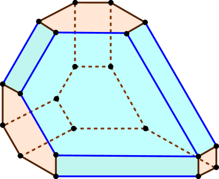
(b) Blue faces collapsed to get $K_{5}$

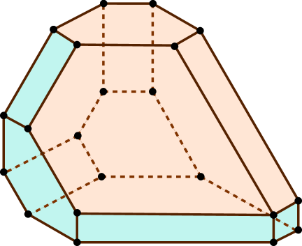
(c) Another degeneration

Figure 6. $\mathcal{J}(4)$ and its degeneration to $K_{5}$

Multiplihedra first appeared in the work of Stasheff [28]. However, in 1986, Norio Iwase and Mamoru Mimura [17, Section 2] gave the first detailed construction of $\mathcal{J}(n)$ with face operators, and described their combinatorial properties. It was also shown that $\mathcal{J}(n)$ is homeomorphic to the unit cube of dimension $n-1$. Using this description of $\mathcal{J}(n)$, they defined $A_{n}$ maps. But even before them, Boardman and Vogt [3] (around 1973) had developed several homotopy equivalent versions of a space of painted binary trees with interior edges of length in $[0,1]$ to define maps between $A_{\infty}$ spaces which preserve the multiplicative structure up to homotopy. In 2008, Forcey [11, Theorem 4.1] proved that the space of painted trees with $n$ leaves, as convex polytopes, are combinatorially equivalent to the CW-complexes described by Iwase and Mimura. Indeed, Forcey associated a co-ordinate to each painted binary trees, which generalized the Loday’s integer coordinates associated to binary trees corresponding to the vertices of associahedra. Figure 6(a) of $\mathcal{J}(4)$ is drawn with such coordinates for the vertices. We shall use the definition of $\mathcal{J}(n)$, as defined in [11], in terms of painted trees.

Definition 2.8.

A painted tree is painted beginning at the root edge (the leaf edges are unpainted), and always painted in such a way that there are only following three types of nodes:

This limitation on nodes implies that painted regions must be connected, that painting must never end precisely at a node of valency three or more, and that painting must proceed up every branches of such nodes.

Let $J(n)$ consist of all painted trees with $n$ leaves. There is a refinement ordering defined as follows.

Definition 2.9.

[11, Definition 1] For $t,t^{\prime}\in J(n)$, we say $t$ refines $t^{\prime}$ and denote by $t\preccurlyeq t^{\prime}$ if $t^{\prime}$ obtained from $t$ by collapsing some of its internal edges.
We say $t$ minimally refines $t^{\prime}$ if $t$ refines $t^{\prime}$ and there is no $s\in J(n)$ such that both $t$ refines $s$ and $s$ refines $t^{\prime}$.

Now $(J(n),\preccurlyeq)$ is a poset with painted binary trees as smallest elements (in the sense that nothing refine them) and the painted corolla as the greatest element (in the sense that everything refines it). The $n$th multiplihedra is defined as follows.

Definition 2.10.

The $n$th multiplihedra $\mathcal{J}(n)$ is a convex polytope whose face poset is isomorphic to the poset $(J(n),\preccurlyeq)$ of painted trees with $n$ leaves.

The explicit inductive construction of these polytopes and the correspondence between the facets of $\mathcal{J}(n)$ and the painted trees follows from [11, Definition 4]. For instance, the vertices of $\mathcal{J}(n)$ are in bijection with the painted binary trees with $n$ leaves; the edges are in bijection with those painted trees with $n$ leaves which are obtained by the minimal refinement of painted binary trees with $n$ leaves and they are glued together along the end points with matching associated to painted binary trees. In this way, the $(n-2)$-dimensional cells of $\mathcal{J}(n)$ are in bijection with those painted trees which refine to corolla with $n$ leaves. They are glued together along $(n-3)$-dimensional cells with matching to associated painted trees to form the complex $\partial\mathcal{J}(n)$. Finally the $(n-1)$ dimensional complex $\mathcal{J}(n)$ is defined as the cone over $\partial\mathcal{J}(n)$ and it corresponds to the painted corolla with $n$ leaves in the poset $J(n)$.

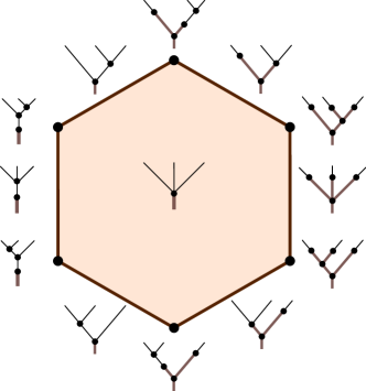
Figure 8. $\mathcal{J}(3)$ labelled by painted trees

We shall give an equivalent description of $\mathcal{J}(n)$ which reflects the promised representation of it stated at the beginning of this subsection. It is given as follows. Let $f:A\to B$ be a weak homomorphism (i.e., respects the multiplication in $A$ and $B$ up to homotopy) from an $A_{\infty}$ space to another $A_{\infty}$ space. For a given ordered collection $a_{1},a_{2},...,a_{n}\in A$, there are three types of elements.

1. The $f$-image of the elements, obtained using different association of the elements $a_{1},a_{2},...,a_{n}$ in $A$. For example, $f(X),$ where $X$ is some rule of association of the elements $a_{1},a_{2},...,a_{n}$.

2. The elements obtained using $f$ being homomorphism up to homotopy on the elements of type I and following the same association rule in $B$. For example, if $X=(X_{1})((X_{2})(X_{3}))$ is some rule of association of $a_{1},a_{2},...,a_{n}$, then elements of the form $f((X_{1})\cdot((X_{2})(X_{3})))$ is of this type. Here $f((X_{1})\cdot((X_{2})(X_{3})))$ denotes the homotopy equivalence between $f((X_{1})((X_{2})(X_{3})))$ and $f(X_{1})f((X_{2})(X_{3}))$. Similarly, $f((X_{1})\cdot((X_{2})\cdot(X_{3})))$, representing the homotopy equivalence between $f((X_{1})(X_{2}\cdot X_{3}))$ and $f(X_{1})f((X_{2})\cdot(X_{3}))$, is also of this type.

3. The elements obtained using different association of the elements of type II in $B$. For example, if $X=(X_{1})((X_{2})((X_{3})(X_{4})))$ is some rule of association of $a_{1},a_{2},...,a_{n}$, then the elements obtained using the different association of $f(X_{1}),f(X_{2}),f(X_{3}),f(X_{4})$ in $B$, namely

   $$(f(X_{1})f(X_{2}))(f(X_{3})f(X_{4})),\ f(X_{1})f(X_{2}) (f(X_{3})f(X_{4})),\ f(X_{1})(f(X_{2})f(X_{3}))f(X_{4}),$$

   $$(f(X_{1})(f(X_{2})f(X_{3})))f(X_{4}), \ f(X_{1})f(X_{2})f(X_{3})f(X_{4})$$

   are of this type.

Definition 2.11.

Let $\mathfrak{J}_{n}$ be the poset of all of the above three types of elements in $B$, ordered such that $P\prec P^{\prime}$ if $P$ is obtained from $P^{\prime}$ by at least one of the following operations:

1. adding brackets in domain or co-domain elements.

2. replacing $\cdot$ by $)f($ without changing the association rule in $P^{\prime}$.

3. removing one or more consecutive $\cdot$ by adding a pair of brackets that encloses all the adjacent elements to all those $\cdot$ which are removed. In this process, ignore redundant bracketing (if obtained). The requirement of consecutive $\cdot$ is to ensure allowable bracketing.

The above operations are to be understood in the following ways:

• For two type I (or III) elements $P,P^{\prime}$, we say $P\prec P^{\prime}$ if $P,P^{\prime}$ follow above operation (1) in domain (or co-domain). For example, $f(a_{1}(a_{2}(a_{3}a_{4})))\prec f(a_{1}(a_{2}a_{3}a_{4})),$ $f(a_{1})(f(a_{2})f(a_{3}a_{4}))\prec f(a_{1})f(a_{2})f(a_{3}a_{4})$.

• For two type II elements $Q,Q^{\prime}$, we say $Q\prec Q^{\prime}$ if $Q,Q^{\prime}$ follow above operation (2) or (3). For example, $f(a_{1})f(a_{2}\cdot(a_{3}a_{4}))\prec f(a_{1}\cdot a_{2}\cdot(a_{3}a_{4})),$ $f(a_{1}\cdot(a_{2}(a_{3}a_{4})))\prec f(a_{1}\cdot(a_{2}\cdot(a_{3}a_{4}))).$

• For type I element $P$ and type II element $Q$, we say $P\prec Q$ if $P,Q$ follow above operation (3).

  For example, $f((a_{1}a_{2})(a_{3}a_{4}))\prec f((a_{1}a_{2})\cdot(a_{3}a_{4})),$ $f(a_{1}a_{2}a_{3}a_{4})\prec f(a_{1}\cdot a_{2}\cdot a_{3}\cdot a_{4})$.

• For type II element $Q$ and type III element $P$, we say $P\prec Q$ if $P,Q$ follow above operation (2) or (3). For example, $(f(a_{1})f(a_{2}a_{3}))f(a_{4})\prec f(a_{1}\cdot(a_{2}a_{3}))f(a_{4}),$ $f(a_{1})(f(a_{2}a_{3})f(a_{4}))\prec f(a_{1})(f(a_{2}\cdot a_{3})f(a_{4}))$.

Now, depending on the poset $(\mathfrak{J}_{n},\prec)$, we define another set of complexes $J_{n}$ for $n\geq 1$.

Definition 2.12.

Define $J_{n}$ to be the convex polytope of dimension $n-1$, whose face poset is isomorphic to $(\mathfrak{J}_{n},\prec)$ for $n\geq 1$.

The existence and the equivalence of these complexes with the multiplihedra follows from the following lemma.

Lemma 2.13.

$J_{n}$ is isomorphic to the multiplihedron $\mathcal{J}(n)$ for any $n\geq 1$.

Proof.

It follows from the definitions of $\mathcal{J}(n)$ and $J_{n}$ that to exhibit an isomorphism between the mentioned complexes, it is enough to provide an isomorphism at the poset level. Define a map $\Phi:J(n)\to\mathfrak{J}_{n}$ as follows.

• Put $a_{1}$ through $a_{n}$ from left to right above the leaves of a painted tree.

• If the leaves corresponding to $a_{k}$ through $a_{l}$ for $1\leq k<l\leq n$ are joined to a node of type 7(a) or of type 7(c), then associate $(a_{k}a_{k+1}\ldots a_{l})$ (cf. figure 9(a)) or $f(a_{k}\cdot a_{k+1}\cdot\ldots\cdot a_{l})$ (cf. figure 9(c)) respectively to that node. In case $1\leq k=l\leq n$, then associate $f(a_{k})$ to the corresponding node.

• Then proceed to the nodes just below the above ones. If a node is of type 7(a) or 7(c) joining $X_{1}$ through $X_{m}$ as associated nodes just above, then associate $(X_{1}X_{2}\ldots X_{m})$ or $f(X_{1}\cdot X_{2}\cdot\ldots\cdot X_{m})$ respectively to that node. If a node is of type 7(b) joining $f(Y_{1})$ through $f(Y_{m})$ as associated nodes just above, then associate $(f(Y_{1})f(Y_{2})\ldots f(Y_{m}))$ to that node (cf. figure 9(b)).

• Continue the above step iii) till the root node of a painted tree.

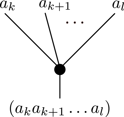
(a)

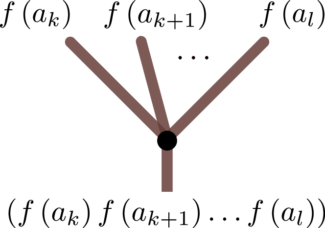
(b)

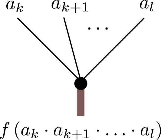
(c)

Figure 9. Bijection between the nodes of painted tree and the elements of defined poset

The element (ignoring redundant brackets, if exists) associated to the root node of a painted tree $t\in J(n)$, is defined to be $\Phi(t)\in\mathfrak{J}_{n}$. For example, the $\Phi$-image of the painted tree $t\in J(5)$ in figure 10 is $f(a_{1}a_{2})(f(a_{3})f(a_{4}\cdot a_{5}))\in\mathfrak{J}_{5}$.
Note that each painted tree is uniquely determined by its nodes and each position of those nodes associates a unique element. Also, the image of $t\in J(n)$ under $\Phi$ is determined by the associated elements to the nodes of $t$. Thus $\Phi$ maps each element of $J(n)$ to a unique element of $\mathfrak{J}_{n}$ and hence $\Phi$ is a bijection.

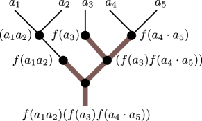
Figure 10. Elements associated to the nodes

It remains to check that $\Phi$ preserves the partial order. By the definition of $\preccurlyeq$, it is enough to show that $\Phi(t)\prec\Phi(t^{\prime})$ when $t\preccurlyeq t^{\prime}$ minimally. If $t\preccurlyeq t^{\prime}$ minimally, then $t^{\prime}$ is obtained from $t$ by collapsing an unpainted internal edge or a painted internal edge or a bunch of painted edges. Note that collapsing an unpainted internal edge results in either removal of brackets in the domain (operation (1) in $\mathfrak{J}_{n}$) or addition of one or more $\cdot$ by removing brackets (operation (3) in $\mathfrak{J}_{n}$). Collapsing a painted internal edge results in removal of brackets in the co-domain (operation (1) in $\mathfrak{J}_{n}$) while collapsing a bunch of painted edges result in replacing $)f($ by $\cdot$ (operation (2) in $\mathfrak{J}_{n}$). In all the cases $\Phi(t)\prec\Phi(t^{\prime})$, completing the proof. ∎

Using this lemma, we consider $J_{n}$ (Definition 2.12) as the $n$th multiplihedron. The pictures of $J_{1},$ $J_{2},$ $J_{3}$ are depicted later in figure 11, with labelling of the faces in terms of elements of $\mathfrak{J}(1)$, $\mathfrak{J}(2)$, $\mathfrak{J}(3)$ respectively.

(a) $J_{1}$

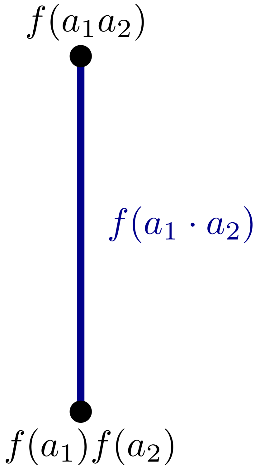
(b) $J_{2}$

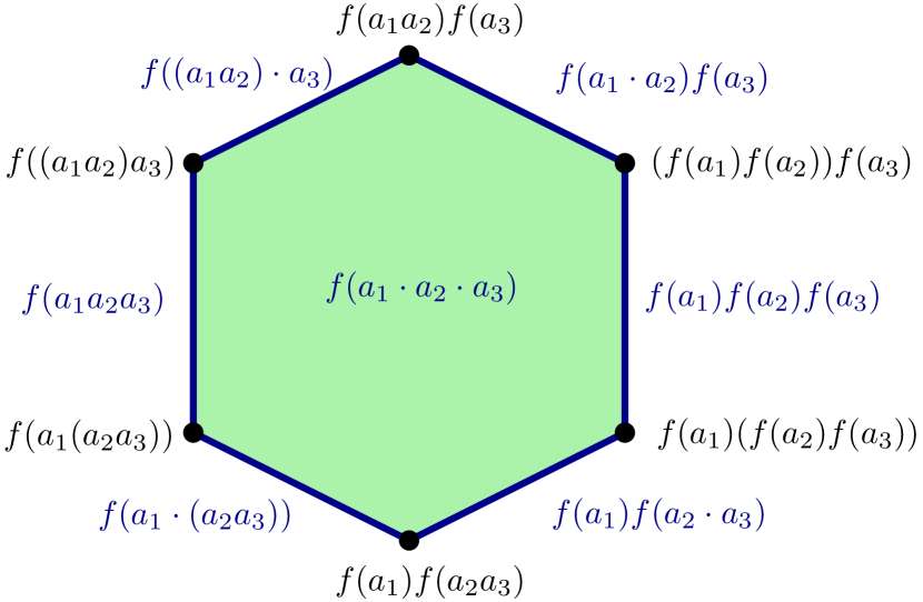
(c) $J_{3}$

Figure 11. Multiplihedra

Now suppose $B$ is an associative space. Due to the associativity in $B$, there will be only one element of type III (as defined before) for each association rule of $a_{1},a_{2},...,a_{n}.$ For example, if $X=((X_{1}X_{2})(X_{3}X_{4}))$ is some association rule of $a_{1},a_{2},...,a_{n}$, then there is only one element $f(X_{1})f(X_{2})$ $f(X_{3})f(X_{4})$ in $B$ using the fact that $f$ is a homomorphism up to homotopy. We will call them degenerate type III elements.

Definition 2.14.

Let $\mathfrak{J}^{\prime}_{n}$ be the poset of all type I, type II, and degenerate type III elements in $B$ with the ordering induced from $(\mathfrak{J}^{\prime}_{n},\prec)$. We define the collapsed multiplihedron $J^{\prime}_{n}$ to be the convex polytope of dimension $n-1$, whose face poset is isomorphic to $\mathfrak{J}^{\prime}_{n}.$

As the posets $\mathfrak{J}^{\prime}_{n}$ are obtained by degeneracy of certain elements in $\mathfrak{J}_{n}$, the polytopes $J^{\prime}_{n}$ are obtained by collapsing certain faces of $J_{n}$. Thus the existence of the polytopes $J^{\prime}_{n}$ guaranteed by the existence of multiplihedron $J_{n}$. We will use this definition to show that $J^{\prime}_{n}$ is combinatorially isomorphic to the associahedron $K_{n+1}$ in §3.2.

2.4. Graph Cubeahedra and Design Tubings

Devadoss [8] gave an alternate definition of $K_{n}$ with respect to tubings on a path graph.

Definition 2.15 (Tube).

Let $\Gamma$ be a graph. A tube is a proper nonempty set of nodes of $\Gamma$ whose induced graph is a proper, connected subgraph of $\Gamma$.

There are three ways that two tubes $t_{1}$ and $t_{2}$ may interact on the graph.

• $t_{1}$ and $t_{2}$ are nested if $t_{1}\subset t_{2}$ or $t_{2}\subset t_{1}$.

  

  Figure 12. Nested tubes

• $t_{1}$ and $t_{2}$ intersect if $t_{1}\cap t_{2}\neq\phi$ and $t_{1}\nsubseteq t_{2}$ and $t_{2}\nsubseteq t_{1}$.

  

  

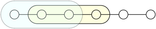
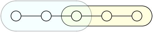
  Figure 13. Intersection of tubes

• $t_{1}$ and $t_{2}$ are adjacent if $t_{1}\cap t_{2}=\phi$ and $t_{1}\cup t_{2}$ is a tube.

  

  

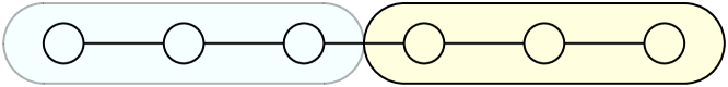
  Figure 14. Adjacent tubes

Two tubes are compatible if they are neither adjacent nor they intersect i.e., $t_{1}$ and $t_{2}$ are compatible if they are nested or $t_{1}\cap t_{2}=\phi$ with $t_{1}\cup t_{2}$ is not a tube.

Definition 2.16.

A tubing $T$ of $\Gamma$ is a set of tubes of $\Gamma$ such that every pair of tubes in $T$ is compatible. A $k$-tubing is a tubing with $k$ tubes.

A few examples of tubings are given below.

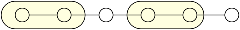
2-tubing

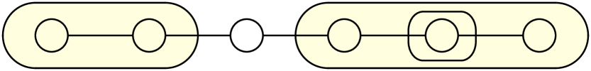
3-tubing

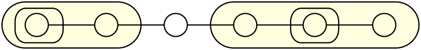
4-tubing

Figure 15. Tubings

If we think of the $n-1$ nodes of a path graph $\Gamma$ as dividers between the $n$ letters of a word and the tube as a pair of parentheses enclosing the letters, then the compatibility condition of the tubes corresponds to the permissible bracketing of word. Now using the combinatorial description (cf. Definition 2.5) of $K_{n}$, one has the following result.

Lemma 2.17.

[5, Lemma 2.3]  Let $\Gamma$ be a path graph with $n-1$ nodes. The face poset of $K_{n}$ is isomorphic to the poset of all valid tubings of $\Gamma$, ordered such that tubings $T\prec T^{\prime}$ if $T$ is obtained from $T^{\prime}$ by adding tubes.

On a graph, Devadoss [8] defines another set of tubes called design tubes.

Definition 2.18 (Design Tube).

Let $G$ be a connected graph. A round tube is a set of nodes of $G$ whose induced graph is a connected (and not necessarily proper) subgraph of $G$. A square tube is a single node of $G$. Then round tubes and square tubes together called design tubes of $G$.

Two design tubes are compatible if

1. they are both round, they are not adjacent and do not intersect;

2. otherwise, they are not nested.

Definition 2.19 (Design Tubing).

A design tubing $U$ of $G$ is a collection of design tubes of $G$ such that every pair of tubes in $U$ is compatible.

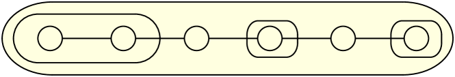
4-design tubing

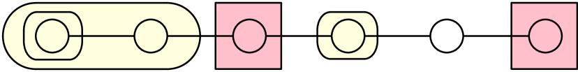
5-design tubing

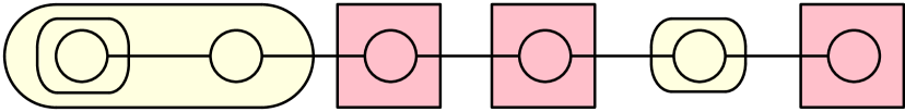
6-design tubing

Figure 16. Design tubings

Note that, unlike ordinary tubes, round tubes do not have to be proper subgraphs of $G$.
     Based on design tubings, Devadoss [8] constructed a set of polytopes called graph cubeahedra. For a graph $G$ with $n$ nodes, define $\boxdot_{G}$ to be the $n$-cube where each pair of opposite facets correspond to a particular node of $G$. Specifically, one facet in the pair represents that node as a round tube and the other represents it as a square tube. Each subset of nodes of $G$, chosen to be either round or square, corresponds to a unique face of $\boxdot_{G}$ defined by the intersection of the faces associated to those nodes. The empty set corresponds to the face which is the entire polytope $\boxdot_{G}$.

Definition 2.20 (Graph Cubeahedron).

For a graph $G$, truncate faces of $\boxdot_{G}$ which correspond to round tubes in increasing order of dimension. The resulting polytope $\mathcal{C}G$ is the graph cubeahedron.

The graph cubeahedron $\mathcal{C}G$ can also be described as a convex polytope whose face poset formed through the design tubings.

Theorem 2.21.

[8, Theorem 12] For a graph $G$ with $n$ nodes, the graph cubeahedron $\mathcal{C}G$ is a simple convex polytope of dimension $n$ whose face poset is isomorphic to the set of design tubings of $G$, ordered such that $U\prec U^{\prime}$ if $U$ is obtained from $U^{\prime}$ by adding tubes.

In this article, we are interested in the case when $G$ is a path graph. We will make use of the above theorem to show a combinatorial isomorphism between $\mathcal{C}G$ for $G$ is a path graph with $n$ nodes and multiplihedra $J_{n+1}$ in §3.3.

3. Isomorphisms Between The Four Models

We prove the main result of this paper in this section.

Theorem 3.1.

The four models of associahedra: Stasheff polytopes, polytopes obtained by Loday’s cone construction, collapsed multiplihedra, graph cubeahedra for path graphs are all combinatorially isomorphic.

Proof.

We prove the isomorphisms in the next three subsections. In §3.1 we prove that the polytopes obtained via the cone construction of Loday are combinatorially isomorphic to the Stasheff polytopes (Theorem 3.2). In §3.2 we prove that the Stasheff polytopes and collapsed multiplihedra are isomorphic (Proposition 3.4). Finally, in §3.3, the isomorphism between the collapsed multiplihedra and graph cubeahedra is shown (Proposition 3.5). Combining all three, we have our required result. ∎

3.1. Loday’s construction vs Stasheff polytopes

By Stasheff’s description, $K_{n+1}$ is the cone over its boundary elements $K_{p}\times_{r}K_{q}$ for $p+q=n+2$, $2\leq p\leq n$ and $r=1,2,\ldots,p.$ On the other hand, consider $C(\widehat{K}_{n})$, where $\widehat{K}_{n}$ consists of the initial $K_{n}$ together with $K_{p+1}\times_{r}K_{q}$ such that $p+q=n+1$, $2\leq p\leq n-1$ and $r=1,2,\ldots,p$. This enlargement $\widehat{K}_{n}$ can be described in terms of bracketing as follows.

• $K_{n}$ corresponds to $0$-bracketing of the word $x_{1}x_{2}\ldots x_{n}$ i.e., the word itself or the trivial bracketing $(x_{1}x_{2}\ldots x_{n})$. The immediate faces i.e., the boundary consists of $K_{p}\times_{r}K_{q}$ with $p+q=n+1$, $2\leq p\leq n-1$ and $r=1,2,\ldots,p$. Now $K_{p}\times_{r}K_{q}$ corresponds to the $1$-bracketing $x_{1}\ldots x_{r-1}(x_{r}\ldots x_{r+q-1})x_{r+q}\ldots x_{n}$.

• The enlargement $\widehat{K}_{n}$ corresponds to the adding of a letter $x_{n+1}$ to the right of the bracketing corresponding to $K_{n}$. Then the bracketing $x_{1}\ldots x_{r-1}(x_{r}\ldots x_{r+q-1})x_{r+q}\ldots x_{n}$ extends to $x_{1}\ldots x_{r-1}(x_{r}\ldots x_{r+q-1})x_{r+q}\ldots x_{n}x_{n+1}$ for each $p,q,r$ such that $p+q=n+1$, $2\leq p\leq n-1$, and $r=1,2,\ldots,p$. Also the initial $K_{n}$ i.e., $(x_{1}x_{2}\ldots x_{n})$ extends to $(x_{1}x_{2}\ldots x_{n})x_{n+1}$, which corresponds to $K_{2}\times_{1}K_{n}$ in $K_{n+1}$.

• Finally one takes cone over the enlarged complex to obtain $K_{n+1}.$

From the above description, $\widehat{K}_{n}$ can be thought of as union of $K_{p}\times_{r}K_{q}$ with $p+q=(n+1)+1$ for $2\leq p\leq n$ and $r=1,2,\ldots,p-1$. Thus $\widehat{K}_{n}$ is a part of the boundary of $K_{n+1}$ (following Stasheff’s description).

Theorem 3.2.

Stasheff polytopes are combinatorially isomorphic to Loday’s cone construction of associahedra.

To prove combinatorial isomorphism between the two mentioned models, we must show bijective correspondence between vertices, edges and faces of each codimension for the both models respecting the adjacencies. But the faces of codimension more than $1$ are contained in the faces of codimension $1$. Thus if we have appropriate bijection between the faces of codimension $1$ respecting the adjacencies for both models, then the resulting models being cone over combinatorially isomorphic codimension $1$ faces, they are combinatorially isomorphic.

Proof of Theorem 3.2.

It is enough to show that the boundary of $K_{n+1}$ in Loday’s construction can be subdivided to match them with the boundary elements $K_{p}\times_{r}K_{q}$ of $K_{n+1}$ in Stasheff model for $p+q=n+2$, $2\leq p\leq n$ and $r=1,\ldots,p$. As observed in the initial discussion, the only missing boundary part of $K_{n+1}$ in Loday’s construction is the union of $K_{p}\times_{p}K_{q}$ for $p+q=n+2$ with $2\leq p\leq n$. Note that all these missing faces are adjacent to a common vertex, which corresponds to the right to left $(n-1)$-bracketing $x_{1}(x_{2}(\ldots(x_{n-1}(x_{n}x_{n+1}))...))$. As there are $\binom{n-1}{n-2}=n-1$ many choices for removing $(n-2)$ brackets from a $(n-1)$-bracketing (that corresponds to the vertices of $K_{n+1}$), each vertex of $K_{n+1}$ is adjacent to exactly $n-1$ faces codimension $1$ of $K_{n+1}$ (by poset description of Stasheff’s $K_{n+1}$). So the vertex corresponding to $x_{1}(x_{2}(\ldots(x_{n-1}(x_{n}x_{n+1}))...))$ is not obtained in $\widehat{K}_{n}$. Now if we consider any other $(n-1)$-bracketing, then there can at most $n-2$ parentheses after $x_{n+1}$. So removing those parentheses along with some others, we can get a $1$-bracketing that do not enclose $x_{n+1}$ i.e., those vertices are adjacent to some $K_{p}\times_{r}K_{q}$ for $p+q=n+2$ and $r=1,2,\ldots,p-1$. Thus any vertex of $K_{n+1}$ except that corresponding to $x_{1}(x_{2}(\ldots(x_{n-1}(x_{n}x_{n+1}))...))$ is present in $\widehat{K}_{n}$. We identify this missing vertex with the coning vertex of Loday’s construction.
     We shall prove that the missing faces of $K_{n+1}$ in $C(\widehat{K}_{n})$ can be realized as a cone over some portion of the boundary of $\widehat{K}_{n}$. Then we will divide the part $C(\partial\widehat{K}_{n})$ accordingly to identify those with the missing faces. We will prove this together with final result by induction on the following statements:

• $Q_{n-3}:$ $K_{p}\times_{r}K_{q}=C\left((\widehat{K}_{p-1}\times_{r}K_{q})\cup(K_{p}\times_{r}\widehat{K}_{q-1})\right)\text{ if }p+q=n+1\text{ and }p,q\geq 3$.

• $P_{n-2}:$ $K_{n}=C\left(\widehat{K}_{n-1}\right)$, $n\geq 3.$

Here the equalities in the statements represent a combinatorial isomorphism. Note that $Q_{n-3}$ is a collection of statements and the index $r$ is actually superfluous. We will use the convention that $\widehat{K}_{1}=\varnothing$, $C(\varnothing)=\{\ast\}$ and allow $p,q\geq 2$. Then $Q_{n-3}$ contains the statement for $K_{n-1}\times_{r}K_{2}$ as well as $K_{2}\times_{r}K_{n-1}$. Moreover, these are equivalent to the statement $P_{n-3}$ since $K_{2}$ is a point and $K_{n-1}\times K_{2}$ is $K_{n-1}$.
     The steps of induction are as follows.

Step 0: Show that $P_{1}$ holds.
Note $K_{2}$ is the convex polytope that parametrizes the binary operation, i.e., it is a point. As a point has no boundary, so $\widehat{K}_{2}$ is also a point and $C(\widehat{K}_{2})$ is an interval. Now $K_{3}$ is the convex polytope that parametrizes the family of $\mathrm{3}$-ary operations that relate the two ways of forming a $\mathrm{3}$-ary operation via a given binary operation. Thus, $K_{3}$ also represents an interval. Here the boundary of $K_{3}$ consist of two points $K_{2}\times_{1}K_{2}$ and $K_{2}\times_{2}K_{2}$. Let us map $K_{2}\times_{1}K_{2}$ and $K_{2}\times_{2}K_{2}$ to $\widehat{K}_{2}$ and the coning point in $C(\widehat{K}_{2})$ respectively. Then we can map the other points of $K_{3}$ linearly to $C(\widehat{K}_{2})$. Thus we get $K_{3}$ and $C(\widehat{K}_{2})$ are combinatorially isomorphic. So $P_{1}$ is true.

Step 1: Assuming that $P_{1}$ through $P_{n-4}$ hold, show that $Q_{n-3}$ holds.
To prove it we will use the following lemma, the proof of which given at the end of this subsection.

Lemma 3.3.

There is a natural homeomorphism

$$C(X)\times C(Y)\equiv C\left((X\times C(Y))\cup(C(X)\times Y)\right),$$

where $x_{0},y_{0}$ are cone points for $C(X),C(Y)$ respectively and $(x_{0},y_{0})$ is the cone point for $C(Z)$, where $Z=(C(X)\times Y)\cup(X\times C(Y))$.

Now assuming $P_{1}$ through $P_{n-4}$, we have $K_{l}=C(\widehat{K}_{l-1})$ for $l=3,4,...,n-2$. Take any $p,q\geq 3$ with $p+q=n+1$ i.e., $p,q$ both ranges through $3$ to $n-2$. So

$$K_{p}\times_{r}K_{q}= \ C(\widehat{K}_{p-1})\times_{r}C(\widehat{K}_{q-1})\ \ (\text{by the assumption})$$

$$= \ C\left((\widehat{K}_{p-1}\times_{r}C(\widehat{K}_{q-1}))\cup(C(\widehat{K}_{p-1})\times_{r}\widehat{K}_{q-1})\right)\ \ (\text{by the Lemma \ref{lemma:CrossCone}})$$

$$= \ C((\widehat{K}_{p-1}\times_{r}K_{q})\cup(K_{p}\times_{r}\widehat{K}_{q-1}))\ \ (\text{by the assumption})$$

This shows that $Q_{n-3}$ is true.

Step 2: Assuming $P_{1}$ through $P_{n-3}$, show that $P_{n-2}$ hold.

As discussed earlier, to prove that $P_{n-2}$ is true, it is enough to show $K_{s}\times_{s}K_{t}$ with $s+t=n+1$ for $s,t\geq 2$ can be obtained from $C(\widehat{K}_{n-1})$. Consider $s,t\geq 2$ with $s+t=n+1$. Then using the conventions $\widehat{K}_{1}=\varnothing$ and $C(\varnothing)=\{*\}$, we can write

$$\ K_{s}\times_{s}K_{t}$$

$$= \ C(\widehat{K}_{s-1})\times_{s}C(\widehat{K}_{t-1})\ (\text{by $P_{1}$ through $P_{n-3}$})$$

$$= \ C\left((\widehat{K}_{s-1}\times_{s}K_{t})\cup(K_{s}\times_{s}\widehat{K}_{t-1})\right)\ (\text{by the Lemma \ref{lemma:CrossCone}})$$

$$= \ C\left(\left\{\bigcup_{(p,q,r)\in V_{s}}\left((K_{p}\times_{r}K_{q})\times_{s}K_{t}\right)\right\}\bigcup\left\{\bigcup_{(p,q,r)\in V_{t}}\left(K_{s}\times_{s}(K_{p}\times_{r}K_{q})\right)\right\}\right)(\text{by definition of }\widehat{K}_{i-1}),$$

$$\text{ where }V_{i}=\{(a,b,c)\in\mathbb{N}^{3}:2\leq a\leq i-1,\ a+b=i+1,\ 1\leq c\leq a-1\},\ i=s,t.$$

Now using equation (2) (in §2.1), we can write

$$(K_{p}\times_{r}K_{q})\times_{s}K_{t}=(K_{p}\times_{s-q+1}K_{t})\times_{r}K_{q}$$

(obtained by substituting $r=p,s=q,t=t,k=r,j=s-q+1$) for the terms in the first set of unions. As $K_{p}\times_{s-q+1}K_{t}$ is a face of $K_{p+t-1}$, so $(K_{p}\times_{s-q+1}K_{t})\times_{r}K_{q}$ is a face of $K_{p+t-1}\times_{r}K_{q}$, which is again a face of $K_{n}$ because for $(p,q,r)\in V_{s}$,

$$(p+t-1)+q=p+q+t-1=s+1+t-1=s+t=n+1.$$

Thus $(K_{p}\times_{r}K_{q})\times_{s}K_{t}$ is a face of $K_{p+t-1}\times_{r}K_{q}$ of codimension $1$. But as $t\geq 2$ and $1\leq r\leq p-1$, so $r<p+t-1$, which implies that the face $K_{p+t-1}\times_{r}K_{q}$ is already present in the enlargement $\widehat{K}_{n-1}$. Thus each term in the first set of unions is already present in $\widehat{K}_{n-1}$.

Similarly, using equation (1), we have the identification

$$K_{s}\times_{s}(K_{p}\times_{r}K_{q})=(K_{s}\times_{s}K_{p})\times_{s+r-1}K_{q}$$

(obtained by substituting $r=s,s=p,t=q,k=r,j=s$) for the terms in the second set of unions. Here $(K_{s}\times_{s}K_{p})\times_{s+r-1}K_{q}$ is a face of $K_{s+p-1}\times_{s+r-1}K_{q}$, which is a face of $K_{n}$ because for $(p,q,r)\in V_{t}$,

$$(s+p-1)+q=s-1+(p+q)=s-1+t+1=s+t=n+1.$$

Thus $(K_{s}\times_{s}K_{p})\times_{s+r-1}K_{q}$ is a face of $K_{s+p-1}\times_{s+r-1}K_{q}$ of codimension $1$. But $r\leq p-1<p$ implies $s+r-1<s+p-1$, which further implies that the face $K_{s+p-1}\times_{s+r-1}K_{q}$ is already present in the enlargement $\widehat{K}_{n-1}$. Thus each term in the second set of unions is also present in $\widehat{K}_{n-1}$.

It follows that all the parts in the unions are present as a part of the boundary of $\widehat{K}_{n-1}$. Thus the cone over that particular part of the boundary of $\widehat{K}_{n-1}$, we will get $K_{s}\times_{s}K_{t}$ for all $s,t\geq 2$ (with $s+t=n+1$). Also these are present as a part of boundary of $C(\widehat{K}_{n-1})$. Therefore we get a bijection between the faces (of codimension $1$) of $K_{n}$ and $\widehat{K}_{n-1}$. Consequently, they are combinatorially isomorphic. So $P_{n-2}$ is true. This completes the induction step as well the proof of the theorem. ∎

Remark 3.1.

In the above isomorphism, we mapped the starting $K_{n}$ to $K_{2}\times_{1}K_{n}$ and the extension of the boundary element $K_{p}\times_{r}K_{q}$ to $K_{p+1}\times_{r}K_{q}$. Similarly we could map the starting $K_{n}$ to $K_{2}\times_{2}K_{n}$ and the extension of the boundary $K_{p}\times_{r}K_{q}$ to $K_{p+1}\times_{r+1}K_{q}$. But if we want to map the starting $K_{n}$ to $K_{n}\times_{r}K_{2}$ ($r=1,2,...,n$), the corresponding extension of boundary $K_{p}\times_{t}K_{q}$ should map to

$$\begin{cases}K_{p}\times_{t}K_{q+1}&\text{if }t\leq r\leq t+q-1\\ K_{p+1}\times_{t}K_{q}&\text{if }r>t+q-1\\ K_{p+1}\times_{t+1}K_{q}&\text{if }r<t.\end{cases}$$

With a slight modification in the above proof, one can similarly prove that this produces an isomorphism. This, in turn, implies that the faces $K_{n}\times_{r}K_{2}$ or $K_{2}\times_{r}K_{n}$ of $K_{n+1}$ are all equivalent from the point of view of Loday’s construction.

We end this subsection with the proof of Lemma 3.3.

Proof of Lemma 3.3.

We will prove the the equality by showing both inclusions. First suppose $(x,y)=t(x_{0},y_{0})+(1-t)(x_{1},y_{1})\in C(Z)$, where $t\in[0,1]$ and $(x_{1},y_{1})\in Z$. Without loss of generality suppose $(x_{1},y_{1})\in C(X)\times Y$ i.e., $x_{1}=t^{\prime}x_{0}+(1-t^{\prime})x^{\prime}_{1}$ for some $t^{\prime}\in[0,1]$ and $x^{\prime}_{1}\in X$. So

$$(x,y)= \ (tx_{0}+(1-t)x_{1},ty_{0}+(1-t)y_{1})$$

$$= \ (tx_{0}+(1-t)t^{\prime}x_{0}+(1-t)(1-t^{\prime})x^{\prime}_{1},ty_{0}+(1-t)y_{1})$$

$$= \ ((1-(1-t)(1-t^{\prime}))x_{0}+(1-t)(1-t^{\prime})x^{\prime}_{1},ty_{0}+(1-t)y_{1})$$

$$= \ (t_{1}x_{0}+(1-t_{1})x^{\prime}_{1},ty_{0}+(1-t)y_{1})\in C(X)\times C(Y)$$

and $t_{1}=1-(1-t)(1-t^{\prime})$. This implies that $C(Z)\subseteq C(X)\times C(Y).$

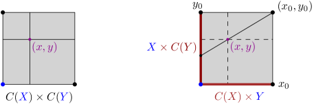
Figure 17. Visual proof when $X=Y=$ point

Conversely let $(x,y)=(t_{1}x_{0}+(1-t_{1})x_{1},t_{2}y_{0}+(1-t_{2})y_{1})\in C(X)\times C(Y)$ for some $x_{1}\in X$, $y_{1}\in Y$ and $t_{1},t_{2}\in[0,1]$. Now consider the following cases
Case I: $t_{1}=t_{2}=t$.

$$(x,y)=t(x_{0},y_{0})+(1-t)(x_{1},y_{1})\in C(Z).$$

Case II: $t_{1}>t_{2}$.

$$(x,y)= \ t_{2}(x_{0},y_{0})+(1-t_{2})\left(\textstyle{\frac{t_{1}-t_{2}}{1-t_{2}}}x_{0}+\textstyle{\frac{1-t_{1}}{1-t_{2}}}x_{1},y_{1}\right)$$

$$= \ t_{2}(x_{0},y_{0})+(1-t_{2})(t^{\prime}x_{0}+(1-t^{\prime})x_{1},y_{1})\in C(Z),$$

$$\ \text{ where }t^{\prime}=\textstyle{\frac{t_{1}-t_{2}}{1-t_{2}}}.$$

Case III: $t_{1}<t_{2}$.

$$(x,y)= \ t_{1}(x_{0},y_{0})+(1-t_{1})\left(x_{1},\textstyle{\frac{t_{2}-t_{1}}{1-t_{1}}}y_{0}+\textstyle{\frac{1-t_{2}}{1-t_{1}}}y_{1}\right)$$

$$= \ t_{1}(x_{0},y_{0})+(1-t_{1})(x_{1},t^{\prime}y_{0}+(1-t^{\prime})y_{1})\in C(Z),$$

$$\ \text{ where }t^{\prime}=\textstyle{\frac{t_{2}-t_{1}}{1-t_{1}}}.$$

Combining all three cases, we conclude that $(x,y)\in C(Z)$ and consequently $C(X)\times C(Y)\subseteq C(Z)$. ∎

3.2. Stasheff polytopes vs Collapsed Multiplihedra

We shall use the Definition 2.5 for Stasheff polytopes. Similarly, due to Lemma 2.13, we will use Definition 2.14 for collapsed multiplihedra.

Proposition 3.4.

Stasheff polytopes $K_{n+1}$ and collapsed multiplihedra $J^{\prime}_{n}$ are combinatorially isomorphic.

Proof.

Both $K_{n+1}$ and $J^{\prime}_{n}$ are convex polytopes whose face posets are isomorphic to $\mathfrak{P}(n+1)$ and $\mathfrak{J}^{\prime}_{n}$ respectively. Therefore, in order to exhibit an isomorphism between $J^{\prime}_{n}$ and $K_{n+1}$, it suffies to find a bijection between $\mathfrak{P}(n+1)$ and $\mathfrak{J}^{\prime}_{n}$ as posets.

Define $\phi:\mathfrak{J}^{\prime}_{n}\to\mathfrak{P}(n+1)$ as follows

$$f(X_{1}) \mapsto f(X_{1})a_{n+1}:=(X_{1})a_{n+1}$$

$$f((X_{1})\cdot\ldots\cdot(X_{k-1})\cdot(X_{k})) \mapsto((X_{1})\cdot\ldots\cdot(X_{k-1})\cdot(X_{k}))a_{n+1}:=(X_{1})\ldots(X_{k-1})(X_{k})a_{n+1}$$

$$\phi\left(f(X_{1})\ldots f(X_{k-1})f(X_{k})\right) =f(X_{1})\ldots f(X_{k-1})f(X_{k})a_{n+1}$$

$$=f(X_{1})\ldots f(X_{k-1})((X_{k})a_{n+1})$$

$$=f(X_{1})\ldots f(X_{k-2})((X_{k-1})((X_{k})a_{n+1}))$$

$$=\cdots$$

$$=(X_{1})(\ldots((X_{k-1})((X_{k})a_{n+1}))\ldots),$$

$$\phi\left(f((X_{1})\cdot(X_{2}))f((X_{3})\cdot(X_{4})\cdot(X_{5}))\right) =f((X_{1})\cdot(X_{2}))(((X_{3})\cdot(X_{4})\cdot(X_{5}))a_{n+1})$$

$$=((X_{1})\cdot(X_{2}))((X_{3})(X_{4})(X_{5})a_{n+1})$$

$$=(X_{1})(X_{2})((X_{3})(X_{4})(X_{5})a_{n+1}).$$

Here $X_{i}$’s are some rule of association of the elements $a_{1},a_{2},...,a_{n}$ in $A$ of some length such that the total length of all $X_{i}$’s is $n$ and $a_{n+1}$ is some different element in $A$. In the above correspondence, note that the bracketing in $X_{i}$’s are not changed. We only include some pair of brackets removing $f$’s or remove $\cdot$ and keep it as it is with an extra letter $a_{n+1}$ on the right to get a bracketing of the word $a_{1}a_{2}\ldots a_{n+1}$. Also, note that each parentheses right to the letter $a_{n+1}$ determines the number of $f$ and their position as well, where no parentheses means only single $f$ with the $\cdot$’s in between the associated words. Thus, the position of each $f$ and $\cdot$ gives a unique bracketing of the word $a_{1}a_{2}\ldots a_{n+1}$ and the process can also be reversed. So $\phi$ is bijective. Now in order to check $\phi$ preserves the poset relation, we need to show $\phi(P\prec P^{\prime})\implies\phi(P)<\phi(P^{\prime}).$ There are three possible ways (cf. operation (1), (2), (3)) by which $P$ can be related to $P^{\prime}$.

1. $P$ is obtained from $P^{\prime}$ by adding brackets in domain. Since $\phi$ do not interact with the brackets in domain, $\phi(P)$ is also obtained from $\phi(P^{\prime})$ by adding brackets i.e., $\phi(P)<\phi(P^{\prime})$.

2. $P$ is obtained from $P^{\prime}$ by replacing $\cdot$ by ‘$)f($’. Thus $P$ contains more $f$ than $P^{\prime}$. But from the correspondence, we know each $f$ corresponds to a pair of bracket, so $\phi(P)$ must be obtained from $\phi(P^{\prime})$ by adding brackets i.e., $\phi(P)<\phi(P^{\prime})$.

3. $P$ is obtained from $P^{\prime}$ by removing one or more consecutive $\cdot$ by adding pair of brackets that encloses all the adjacent elements to those $\cdot$. To obtain $P$, this process adds brackets to $P^{\prime}$ and $\phi$ does not change the parent bracketing. So so $\phi(P)$ must be obtained from $\phi(P^{\prime})$ by adding brackets i.e., $\phi(P)<\phi(P^{\prime})$.

Thus $\phi$ defines a bijection of the posets $\mathfrak{J}^{\prime}_{n}$ and $\mathfrak{P}(n+1)$. Hence $J^{\prime}_{n}$ and $K_{n+1}$ are combinatorially isomorphic. ∎

3.3. Collapsed Multiplihedra vs Graph Cubeahedra

Proposition 3.5.

Collapsed multiplihedra $J^{\prime}_{n+1}$ and graph cubeahedra $\mathcal{C}P_{n}$ for path graph $P_{n}$ with $n$ nodes are combinatorially isomorphic.

Proof.

Recall from Theorem 2.21 that the graph cubeahedron $\mathcal{C}P_{n}$ is a convex polytope of dimension $n$ whose face poset is isomorphic to the set of design tubings of $P_{n}$. Recall that the collapsed multiplihedra $J^{\prime}_{n+1}$ is a convex polytope of dimension $n$ whose face poset is isomorphic to $\mathfrak{J}^{\prime}_{n+1}$. Thus, to describe an isomorphism, it is enough to prove a bijection at the poset level.
     A bijection between the design tubings and the elements of $\mathfrak{J}^{\prime}_{n+1}$ is defined through the following correspondences:

• Put $a_{1}$ through $a_{n+1}$ starting from the left of the left-most node to the right of the right-most node of the graph:

  

  Figure 18. Initial step

• Each round tube corresponds to a pair of parentheses. If the round tube include $k$-th and $(k+r-1)$-th node of the graph, then the corresponding parentheses include $a_{k}$ through $a_{k+r}$.

  

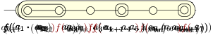
  Figure 19. Correspondence of round tube

• Each square tube corresponds to the inclusion of ‘$)f($’ in the string $f(a_{1}a_{2}\ldots a_{n+1})$. If the square tube include $k$-th node of the graph, then ‘$)f($’ will be included in between $a_{k}$ and $a_{k+1}$.

  

  Figure 20. Correspondence of square tube

• An empty node in a tubing corresponds to ‘$\cdot$’ i.e., if $k$-th node of the graph is not included by any tube of the given tubing, then put a ‘$\cdot$’ between $a_{k}$ and $a_{k+1}$.

  

  Figure 21. Correspondence of empty node

Finally as position of each tube and its appearance give a unique element of $\mathfrak{J}^{\prime}_{n+1}$, we get a bijective correspondence between design tubings and elements of $\mathfrak{J}^{\prime}_{n+1}.$ An example, assuming $n=6$, is given below.

Figure 22. Bijection between design tubings and multiplihedra

It follows from the correspondence that the removal of a round tube corresponds to removal of a pair of parentheses or adding ‘$\cdot$’ and the removal of a square tube corresponds to replacing ‘$)f($’ by ‘$\cdot$’. This shows that the poset relation between design tubings match with the poset relation in $\mathfrak{J}^{\prime}_{n+1}.$ As the two posets are isomorphic, this finishes the proof. ∎

References

- [1] J. F. Adams, Infinite loop spaces, Annals of Mathematics Studies, No. 90, Princeton University Press, Princeton, N.J.; University of Tokyo Press, Tokyo, 1978.
- [2] N. Arkani-Hamed, Y. Bai, S. He, and G. Yan, Scattering forms and the positive geometry of kinematics, color and the worldsheet, J. High Energy Phys., (2018), pp. 096, front matter+75.
- [3] J. M. Boardman and R. M. Vogt, Homotopy invariant algebraic structures on topological spaces, Lecture Notes in Mathematics, Vol. 347, Springer-Verlag, Berlin-New York, 1973.
- [4] G. Bowlin and M. G. Brin, Coloring planar graphs via colored paths in the associahedra, Internat. J. Algebra Comput., 23 (2013), pp. 1337–1418.
- [5] M. P. Carr and S. L. Devadoss, Coxeter complexes and graph-associahedra, Topology Appl., 153 (2006), pp. 2155–2168.
- [6] S. Devadoss and S. Forcey, Marked tubes and the graph multiplihedron, Algebraic and Geometric Topology, 8 (2008), p. 2081–2108.
- [7] S. L. Devadoss, Tessellations of moduli spaces and the mosaic operad, 239 (1999), pp. 91–114.
- [8] S. L. Devadoss, T. Heath, and W. Vipismakul, Deformations of bordered surfaces and convex polytopes, Notices Amer. Math. Soc., 58 (2011), pp. 530–541.
- [9] L. Ferro and T. Ł ukowski, Amplituhedra, and beyond, J. Phys. A, 54 (2021), pp. Paper No. 033001, 42.
- [10] S. Fomin and A. Zelevinsky, -systems and generalized associahedra, Ann. of Math. (2), 158 (2003), pp. 977–1018.
- [11] S. Forcey, Convex hull realizations of the multiplihedra, Topology Appl., 156 (2008), pp. 326–347.
- [12] , Quotients of the multiplihedron as categorified associahedra, Homology Homotopy Appl., 10 (2008), pp. 227–256.
- [13] , Extending the Tamari lattice to some compositions of species, in Associahedra, Tamari lattices and related structures, vol. 299 of Progr. Math., Birkhäuser/Springer, Basel, 2012, pp. 187–210.
- [14] K. Fukaya and Y.-G. Oh, Zero-loop open strings in the cotangent bundle and Morse homotopy, Asian J. Math., 1 (1997), pp. 96–180.
- [15] M. Haiman, Constructing the associahedron, 1984. available at https://math.berkeley.edu/~mhaiman/ftp/assoc/manuscript.pdf.
- [16] D. Huguet and D. Tamari, La structure polyédrale des complexes de parenthésages, J. Combin. Inform. System Sci., 3 (1978), pp. 69–81.
- [17] N. Iwase and M. Mimura, Higher homotopy associativity, in Algebraic topology (Arcata, CA, 1986), vol. 1370 of Lecture Notes in Math., Springer, Berlin, 1989, pp. 193–220.
- [18] B. Keller, Introduction to -infinity algebras and modules, Homology Homotopy Appl., 3 (2001), pp. 1–35.
- [19] C. W. Lee, The associahedron and triangulations of the -gon, European J. Combin., 10 (1989), pp. 551–560.
- [20] J.-L. Loday, Realization of the Stasheff polytope, Arch. Math. (Basel), 83 (2004), pp. 267–278.
- [21] , The multiple facets of the associahedron, 2005. available at https://citeseerx.ist.psu.edu/viewdoc/download?doi=10.1.1.297.9348&rep=rep1&type=pdf.
- [22] S. Mau and C. Woodward, Geometric realizations of the multiplihedron and its complexification, 2009.
- [23] J. P. May, The geometry of iterated loop spaces, Lecture Notes in Mathematics, Vol. 271, Springer-Verlag, Berlin-New York, 1972.
- [24] S. Mizera, Combinatorics and topology of Kawai-Lewellen-Tye relations, J. High Energy Phys., (2017), pp. 097, front matter+53.
- [25] L. Pournin, The diameter of associahedra, Adv. Math., 259 (2014), pp. 13–42.
- [26] S. Saneblidze and R. Umble, Diagonals on the permutahedra, multiplihedra and associahedra, Homology Homotopy Appl., 6 (2004), pp. 363–411.
- [27] D. D. Sleator, R. E. Tarjan, and W. P. Thurston, Rotation distance, triangulations, and hyperbolic geometry, J. Amer. Math. Soc., 1 (1988), pp. 647–681.
- [28] J. Stasheff, -spaces from a homotopy point of view, Lecture Notes in Mathematics, Vol. 161, Springer-Verlag, Berlin-New York, 1970.
- [29] J. D. Stasheff, Homotopy associativity of -spaces. I, II, Trans. Amer. Math. Soc. 108 (1963), 275-292; ibid., 108 (1963), pp. 293–312.
- [30] M. Sugawara, On a condition that a space is an -space, Math. J. Okayama Univ., 6 (1957), pp. 109–129.
- [31] , On the homotopy-commutativity of groups and loop spaces, Mem. Coll. Sci. Univ. Kyoto Ser. A. Math., 33 (1960/61), pp. 257–269.
- [32] D. Tamari, Monoïdes préordonnés et chaînes de malcev, Bulletin de la Société Mathématique de France, 82 (1954), pp. 53–96.