A novel nonperturbative renormalization scheme for local operators

Abstract

The gradient flow exponentially suppresses ultraviolet field fluctuations and removes ultraviolet divergences (up to a multiplicative fermionic wavefunction renormalization). It can be used to describe real-space Wilsonian renormalization group transformations and determine the corresponding beta function. We propose a new nonperturbative renormalization scheme for local composite fermionic operators that uses the gradient flow and is amenable to lattice QCD calculations. We present preliminary nonperturbative results for the running of quark bilinear operators in this scheme and outline the calculation of perturbative matching to the $\overline{\mathrm{MS}}$ scheme.

1 Introduction

Quantum chromodynamics (QCD), the gauge theory of the strong nuclear force, is strongly coupled at hadronic energy scales. Lattice QCD provides a numerical approach to studying the nonperturbative features of QCD by discretizing spacetime and evaluating the path integral stochastically with Markov chain Monte Carlo methods. The discretized spacetime provides a gauge-invariant ultraviolet regulator of QCD, and taking the continuum limit corresponds to removing this ultraviolet regulator. This, in turn, requires that both the lattice QCD action and all probe operators are renormalized. For QCD at hadronic energy scales, this requires a nonperturbative renormalization procedure. Ideally, a fully nonperturbative renormalization scheme for lattice QCD should preserve gauge-invariance and be amenable to numerical implementation on the lattice and calculable in perturbation theory at high energies. Moreover, a method for extracting the nonperturbative energy dependence that allows matching results in both low- and high-energy regimes is necessary. We propose a new renormalization procedure that satisfies these requirements and study its application to quark bilinear operators.

This new approach allows for the nonperturbative determination of the anomalous dimension of quark bilinear operators through the real-space renormalization group (RG), implemented using the gradient flow [1, 2, 3]. The gradient flow is not an RG transformation as it lacks the crucial step of rescaling (coarse graining). However, as Ref. [4] outlines, a coarse graining step can be implemented at the level of expectation values, transforming the gradient flow to a complete real-space RG transformation. There are three steps. First, we calculate the nonperturbative renormalization parameter $Z_{\mathcal{O}}^{\mathrm{GF}}(\mu,a)$ at a low-energy scale, through a ratio of matrix elements of gradient-flowed operator ${\mathcal{O}}$. Then, we evaluate the nonperturbative anomalous dimension, $\gamma_{\mathcal{O}}$ by computing the numerical logarithmic derivative of $Z_{\mathcal{O}}^{\mathrm{GF}}(\mu,a)$. Finally we match the nonperturbative gradient flow scheme to the $\overline{\mathrm{MS}}$-scheme (or similar) at high energy, using a short flow time expansion (SFTE) applied to our gradient flow scheme.

There are two widely-used nonperturbative renormalization schemes in lattice QCD, the Schrödinger functional [5, 6], and regularization-independent momentum subtraction (RI/MOM) schemes [7]. On the one hand, the Schrödinger functional approach is gauge-invariant and provides a natural definition of a finite volume scheme that enables the extraction of the nonperturbative running of operators, but at the cost of introducing additional analytic complications. On the other hand, RI/MOM schemes break gauge invariance, which introduces computational challenges for the gauge sector, and do not provide a natural step-scaling procedure to match low and high energy regimes. A previous proposal to use the gradient flow to define a renormalization scheme for local fermionic operators was limited to a finite volume step-scaling procedure for quenched QCD [8].

Our proposed scheme is gauge invariant and defines anomalous dimensions nonperturbatively. However, the smearing radius of the flow must be small compared to other length scales in the calculation, which may lead to a “window problem”. Moreover, the flow introduces additional diagrams in perturbative matching calculations. We note that these diagrams can be computed in continuum perturbation theory, avoiding the need for lattice perturbation theory.

Here we provide a proof-of-principle calculation of the renormalization factors and anomalous dimensions of quark bilinear operators. We anticipate that our renormalization scheme can be implemented for a wide range of local operators in lattice QCD, from flavor-changing weak currents and four-quark operators, to twist-2 operators relevant to hadron structure calculations. Calculations for further quantities are discussed in [9, 10, 11, 12, 13]. Future work will be required to identify the region of applicability, quantify the associated systematic uncertainties, and assess the viability of our scheme for different local operators.

2 Renormalization procedure

Gradient flow transformations can describe real-space Wilsonian RG transformations [4, 14, 15, 16, 17, 18], allowing the determination of the RG $\beta$ function of the running coupling constant [19, 20, 21, 22, 23] and the anomalous dimension of composite fermion operators [4].

Real space RG transformations are constructed from blocked fields, defined over a “coarse-grained" subset of the lattice and constructed from the original fields, which are then integrated out. Blocking transformations leave the partition function of the theory invariant, but both the parameters of the action and expectation values of operators change. Typically, these changes have a complicated analytical form, but in the vicinity of a fixed point or renormalized trajectory the analytic structure is well understood.

The gradient flow transformation in real space averages the field variables over a region proportional to $\sqrt{2Dt}$ in a $D$-dimensional spacetime [2, 3, 1]. The flowed fields are therefore a natural choice for blocked field variables. Moreover, flowed operators provide probes of unflowed composite operators. So it is natural to consider correlation functions between blocked and unblocked, flowed and unflowed operators. The gradient flow transformation does not change the lattice spacing, it has to be supplemented by a coarse graining step to define an RG transformation. Coarse graining can be applied to expectation values. That way the gradient flow describes an RG transformation if the gradient flow flow-time $t$ and RG scale change $b$ are related by $b\propto\sqrt{t/a^{2}}$, with $\sqrt{t/a^{2}}\gg 1$ [4].

Calculating expectation values in RG flowed systems does not require simulations with the flowed action. It is sufficient to calculate expectation values of flowed operators on ensembles generated with the original action. This observation greatly simplifies the numerical task of real space RG [24]. Nevertheless, it is worth emphasizing that the gradient flow is not an RG transformation. The RG blocked action has fixed points, while the flowed action flows to a saddle in the action parameter space. Moreover, identifying flowed fields with blocked fields does not allow the iteration of the RG transformation, because the blocked fields from a second blocking step cannot be expressed as simple flowed variables.

In the large flow-time limit the RG flow tracks the renormalized trajectory and expectation values of scaling operators describe continuum physics. In particular, the operator $t^{2}\langle E\rangle_{t}$, where $\langle E\rangle_{t}$ is the energy density of the gauge fields at flow time $t$, is dimensionless and can be used to define a renormalized coupling and the corresponding RG $\beta$ function,

$$g^{2}_{\mathrm{GF}}(t/a^{2};\beta)=\mathcal{N}t^{2}\langle E\rangle_{t;\beta}\,,\quad\quad\beta(g^{2}_{\text{GF}})=-t\frac{dg^{2}_{\text{GF}}}{d\,t}\,.$$ (1)

The expectation value $\langle E\rangle_{t}$ is calculated on ensembles with fixed bare coupling $\beta=2N_{c}/g_{0}^{2}$ and corresponding lattice spacing $a(\beta)$, so $g^{2}_{\mathrm{GF}}$ depends both on the lattice flow time $t/a^{2}$ and $\beta$. Here ${\cal N}$ is a normalization and throughout this work we use a subscript GF to indicate a gradient flow scheme. Only in the $t/a^{2}\to\infty$ limit can $g^{2}_{\mathrm{GF}}$ be interpreted as a renormalized coupling at energy $\mu\sim 1/\sqrt{8t}$.

Fermionic composite operators evolve according to their scaling dimension under RG. If the RG transformation is linear, as it is the case for the fermion gradient flow [25, 26], they also pick up a wave function renormalization factor $Z_{\chi}$ (corresponding to the $\eta$ exponent in RG language). The vector current has vanishing anomalous dimension, therefore the ratio of any meson operator and the vector current depends only on the anomalous dimension of the meson operator.

To define our renormalization scheme, we consider a local flowed operator ${\mathcal{O}}(x;t/a^{2})$ at fixed bare gauge coupling $\beta$, and its correlation function with a probe operator, $\widetilde{{\mathcal{O}}}$, chosen to ensure that the two-point function

$$G_{\mathcal{O}}(x_{4};t/a^{2},\beta)=a^{3}\sum_{{\bf x}}\left\langle{\mathcal{O}}({\bf x},x_{4};t/a^{2})\widetilde{{\mathcal{O}}}(0)\right\rangle_{\beta}\,$$ (2)

does not vanish. It is natural to chose the unflowed operator as the probe $\widetilde{{\mathcal{O}}}={\mathcal{O}}$.

We define the ratio

$$R_{\mathcal{O}}(x_{4};t/a^{2},\beta)=\frac{G_{\mathcal{O}}(x_{4};t/a^{2},\beta)}{G_{V}(x_{4};t/a^{2},\beta)}\,,$$ (3)

with

$$G_{V}(x_{4};t/a^{2},\beta)=\frac{1}{3}\sum_{k=1}^{3}a^{3}\sum_{{\bf x}}\left\langle V_{k}({\bf x},x_{4};t/a^{2})\widetilde{V}_{k}(0)\right\rangle_{\beta}\,.$$ (4)

Here $V_{k}({\bf x},x_{4};t/a^{2})$ is the vector current defined at lattice flow time $t/a^{2}$ and $\widetilde{V}$ is an appropriate probe operator. The ratio $R_{\mathcal{O}}(x_{4};t/a^{2},\beta)$ depends on the anomalous dimension of the operator ${\mathcal{O}}$ and, in the limit $t/a^{2}\to\infty$, the logarithmic derivative of $R_{\mathcal{O}}(x_{4};t/a^{2},\beta)$ predicts the anomalous dimension

$$\gamma_{\mathcal{O}}(t/a^{2},\beta)=-2t\frac{\mathrm{d}\,\text{log}R_{\mathcal{O}}(x_{4};t/a^{2},\beta)}{\mathrm{d}\,t}\,,\quad\quad x_{4}\gg\sqrt{2Dt}\,.$$ (5)

The condition $x_{4}\gg\sqrt{2Dt}$ ensures that the flowed operator and its probe are well separated, and the correlation function in Eq. (2) decays with an exponent independent of $t/a^{2}$. In this limit $\gamma_{\mathcal{O}}$ is independent of $x_{4}$.

The quantity $\gamma_{\mathcal{O}}(t/a^{2},\beta)$ could be translated to the energy-dependent running anomalous dimension $\gamma_{\mathcal{O}}(\mu)$, but it is easier and more useful to express $\gamma_{\mathcal{O}}(t/a^{2},\beta)$ in terms of the running gauge coupling. Eq. (1) gives the running gauge coupling at lattice flow time $t/a^{2}$ at bare gauge coupling $\beta$, while Eq. (5) predicts the anomalous dimension at the same parameters. Combining the two equations therefore predicts $\gamma_{\mathcal{O}}(g^{2}_{\mathrm{GF}}(t/a^{2},\beta))$. The continuum limit corresponds to $t/a^{2}\to\infty$ at fixed $g^{2}_{\mathrm{GF}}$. That is equivalent to the $\beta\to\infty$ limit, and predicts the running anomalous dimension $\gamma_{\mathcal{O}}(g^{2}_{\mathrm{GF}})$ in the continuum. Once the RG anomalous dimensions and $\beta$ function are known, the expression

$$\exp\int_{\bar{g}_{\mathrm{IR}}}^{\bar{g}_{\mathrm{UV}}}dg^{\prime}~{}\frac{\gamma_{\mathcal{O}}^{\mathrm{GF}}(g^{\prime})}{\beta^{\mathrm{GF}}(g^{\prime})}\,$$ (6)

connects the infrared renormalization factor to its ultraviolet counterpart. If we wish to connect with the $\overline{\mathrm{MS}}$ scheme, a perturbative calculation has to be carried out.

The equivalence of gradient flow and real-space RG is valid in the infinite volume limit. The definition of the renormalized coupling and RG $\beta$ function in Eq. (1) and the anomalous dimension in Eq. (5) require not only infinite volume but also vanishing fermion mass $am_{q}=0$. Thus the continuum renormalization group $\beta$ and $\gamma$ functions are obtained in the $L\to\infty$, $m_{q}\to 0$, $t/a^{2}\to\infty$ limit at fixed renormalized coupling $g^{2}_{\text{GF}}$.

3 Preliminary results

3.1 Nonperturbative calculation

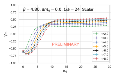
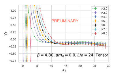
Figure 1: The logarithmic derivative of ratio $R_{\mathcal{O}}$, Eqs. (3) and (5), as a function of the separation $x_{4}$ on the $\beta=4.80$, $am_{q}=0.0$, $24^{3}\times 64$ ensemble. The left panel shows the mass (based on the pseudoscalar operator) and the right the tensor anomalous dimensions. In each case seven flow time values $t/a^{2}\in(2.0,8.0)$ are shown.

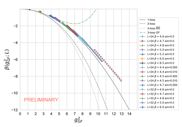
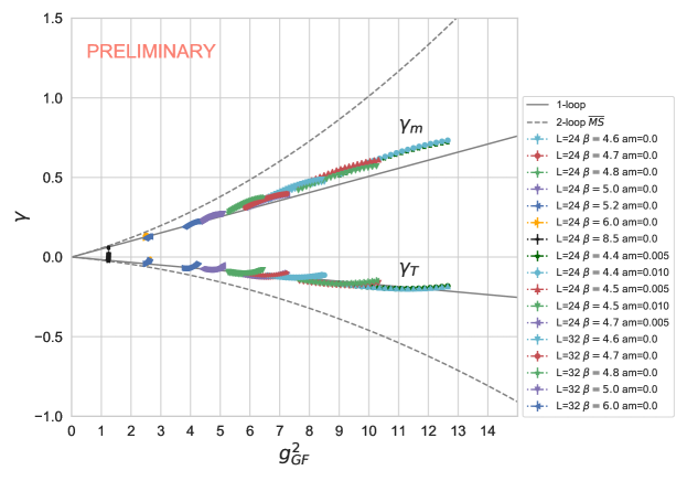
Figure 2: “Raw data” for the RG $\beta$ function (top panel) and mass and tensor anomalous dimensions (bottom panel) as a function of $g^{2}_{\text{GF}}$ at many different bare coupling $\beta$ values obtained for our $N_{f}=2$ simulations. On both panels flow times $t/a^{2}\in(2.0,4.0)$ are shown on $24^{4}\times 64$ and $32^{3}\times 64$ volumes. Simulations in the weak coupling deconfined regime are done in the chiral limit. In the confining regime we use fermion masses $am_{q}=0.005$ and 0.010. Results in the top panel are based on Wilson flow and Wilson operator. We compare our results to the universal perturbative results at one- and two-loop, as well as three-loop in the $\overline{\mathrm{MS}}$ and GF schemes [27]. (For further details see [19].) In the bottom panel we show the universal one-loop and the two-loop $\overline{\mathrm{MS}}$ predictions.

We demonstrate our new renormalization procedure by performing fermionic gradient flow measurements using a set of gauge field ensembles [19] generated with tree-level improved Symanzik (Lüscher-Weisz) $SU(3)$ gauge action [28, 29] and two dynamical flavors of stout-smeared [30] Möbius domain wall fermions [31]. In the deconfined region, we perform simulations at zero quark mass and bare gauge couplings $\beta$ in the range $8.50\geq\beta\geq 4.60$ using volumes $\left(L/a\right)^{3}\times T/a=24^{3}\times 64$ and $32^{3}\times 64$. In addition we generated new $24^{3}\times 64$ ensembles in the confined region with mass $am_{q}=0.005$ and $0.010$ at $\beta=4.40$ and 4.50, and $am_{q}=0.005$ at $\beta=4.70$. All configurations are generated using GRID [32] and we implemented our fermionic gradient flow measurements using QLUA [33]. We choose to use the Wilson kernel with step-size $\epsilon=0.01$ for our gradient flow implementation and apply the Laplace operator to evolve the fermion fields in flow time.

Domain wall fermions preserve chiral symmetry when the fifth dimension $L_{s}$ is infinite. The explicit symmetry breaking for finite $L_{s}$ is characterized by the residual mass $am_{\text{res}}$. In our simulations we keep $L_{s}$ large so $am_{\text{res}}<10^{-6}$. We find that simulations in the small volume weak coupling regime preserve chiral symmetry at the level of statistical fluctuations. This ensures, e.g., that the scalar and pseudoscalar anomalous dimensions are identical, $\gamma_{\text{S}}=\gamma_{\text{PS}}$. We have verified this expectation explicitly.

In Fig. 1 we illustrate that $\gamma_{\mathcal{O}}(t/a^{2},\beta)$ is independent of $x_{4}$, the separation between the flowed operator and the probe, if $x_{4}\gg\sqrt{2Dt}$. The left panel shows the logarithmic derivative defined in Eq. (5) for the pseudoscalar operator on the $\beta=4.80$, $am_{q}=0.0$, $24^{3}\times 64$ ensemble as the function of $x_{4}$. The various color symbols correspond to different flow times between $t/a^{2}=2.0$ and 8.0. While at short distances the flow clearly influences the prediction, all $x_{4}$ dependence vanishes once $x_{4}\gtrsim 2\sqrt{2Dt}$. We use this regime to predict $\gamma_{\mathcal{O}}(t/a^{2},\beta)$. Figure 1 also illustrates the flow time dependence of $\gamma_{\mathcal{O}}$. For the pseudoscalar operator it shows a steady decrease with $t/a^{2}$, indicating that the mass anomalous dimension $\gamma_{m}\equiv\gamma_{\text{S}}=\gamma_{\text{PS}}$ increases with decreasing energy. The right panel shows $\gamma_{\mathcal{O}}$ for the tensor operator. Here we observe a negative anomalous dimension that is decreasing with increasing $t/a^{2}$.

Figure 2 shows our preliminary results for the RG $\beta$ function and for the scalar and tensor anomalous dimensions. Each set of colored symbols correspond to different ensembles and represent the raw data in the flow time range $t/a^{2}\in(2.0,4.0)$. (Larger flow times correspond to larger $g^{2}_{\text{GF}}$ in all cases.) We observe only mild mass dependence. The data at $am_{q}=0.0$, 0.005 and 0.010, when available, are nearly identical. The same is true for the volume dependence. In the investigated flow time range, $L/a=24$ and 32 are barely distinguishable. This implies that the infinite volume and chiral limits will be very similar to the raw data. We emphasize that, more importantly, different bare couplings, covering the range of renormalized couplings $1.0\leq g^{2}_{\text{GF}}\leq 12.0$, map out (approximately) a single curve. Deviations at small $t/a^{2}$ flow time would imply cut-off effects, whereas deviations at large flow time indicate finite volume effects. At fixed $g^{2}_{\text{GF}}$ values we might have predictions from several different ensembles, i.e. different $t/a^{2}$ flow time values. The closeness/overlap of these predictions suggests that the continuum limit $t/a^{2}\to\infty$ extrapolation will also be very similar to the raw data. It is noteworthy that both the scalar and tensor anomalous dimensions lie close to the 1-loop perturbative curve even in the strong coupling range. The $\beta$-function shows similar behavior, pointed out previously in [20, 23].

Once the continuum $\beta$ function and anomalous dimensions are obtained, the ratio of the $Z$ factors can be determined according to Eq. (6). The final step is the perturbative calculation to connect our gradient flow scheme to the $\overline{\mathrm{MS}}$ scheme.

3.2 Perturbative matching at leading order

The matching factor relating our gradient flow scheme and the $\overline{\mathrm{MS}}$ scheme can be written in terms of the renormalization group invariant (RGI) operators as

$$c^{\overline{\mathrm{MS}}\leftarrow\mathrm{GF}}(\mu^{\mathrm{GF}}_{\mathrm{UV}},\mu^{\overline{\mathrm{MS}}}_{\mathrm{UV}}) =\exp\bigg{\{}-\int_{0}^{g_{\mathrm{GF}}^{\mathrm{UV}}}dg^{\prime}~{}\frac{\gamma_{\mathcal{O}}^{\mathrm{GF}}(g^{\prime})}{\beta^{\mathrm{GF}}(g^{\prime})}+\int_{0}^{g_{\overline{\mathrm{MS}}}^{UV}}dg^{\prime}~{}\frac{\gamma_{\mathcal{O}}^{\overline{\mathrm{MS}}}(g^{\prime})}{\beta^{\overline{\mathrm{MS}}}(g^{\prime})}\bigg{\}}\,.$$ (7)

Here we denote the renormalized coupling in the $\overline{\mathrm{MS}}$ scheme by $g_{\overline{\mathrm{MS}}}$ and the renormalized coupling in the $\mathrm{GF}$ scheme by $g_{\mathrm{GF}}$. In general we consider different renormalization scales, $\mu^{\mathrm{GF}}_{\mathrm{UV}},\mu^{\overline{\mathrm{MS}}}_{\mathrm{UV}}$, in the two schemes, both in the perturbative high energy region.

We demonstrate our perturbative matching procedure at leading order in perturbation theory. We determine the next-to-leading-order contributions to the quark bilinear two-point functions, $R_{\mathcal{O}}(x_{4};0)$, by calculating the relevant diagrams at nonzero external momentum transfer and then Fourier transforming the result with respect to the external three momentum. For the leading order anomalous dimension, it is sufficient to determine the flow time dependence of $R_{\mathcal{O}}(x_{4};t)$ through a short flow time expansion of renormalized two-point functions [25]

$$G_{\mathcal{O}}^{R}(x_{4};\mu^{2},t)\sim c_{\mathcal{O}}(\mu^{2}t)G_{\mathcal{O}}^{R}(x_{4};\mu^{2},t=0)+O(t)\,.$$ (8)

This approach has the advantage that the expansion coefficient $c_{\mathcal{O}}(\mu^{2}t)$ can be extracted from a more straightforward one loop calculation of, e.g., quark bilinears with external quark states.

We need only the divergent contributions to $R_{\mathcal{O}}(x_{4};t)$ to extract the leading order anomalous dimension of the quark bilinear ${\mathcal{O}}$. Up to finite terms, the two-point functions are

$$G_{\mathcal{O}}(x_{4};t)=G_{\mathcal{O}}^{(0)}(x_{4};t)\bigg{\{}1-\frac{g^{2}}{12\pi^{2}}\left[\frac{a_{\mathcal{O}}}{\epsilon}+b_{\mathcal{O}}\log(8\pi\mu^{2}t)+c_{\mathcal{O}}\log(\pi\mu^{2}x_{4}^{2})\right]+\mathcal{O}(\epsilon,m,\alpha_{S}^{2})\bigg{\}},$$ (9)

where the $a_{\mathcal{O}}$, $b_{\mathcal{O}}$, and $c_{\mathcal{O}}$ depend on the choice of quark bilinear.

From these results, we evaluate the anomalous dimensions for each quark bilinear through Eq. (5), and find $\gamma_{\mathcal{O}}=g^{2}/(12\pi^{2})\,\{6,6,0,0,-2\}+{\cal O}(g^{4})$ for the scalar, pseudoscalar, vector, axialvector, and tensor currents, respectively. These values are in agreement with [34, 35] in the cases of the scalar and pseudoscalar currents by comparison with the mass anomalous dimension. A complete next-to-leading order matching calculation will be pursued in future work.

4 Summary

We propose a new nonperturbative, gauge-invariant renormalization scheme for local operators in QCD. Our scheme is based on the properties of a real-space renormalization group transformation that we implement through the gradient flow. Here we applied this scheme to local quark bilinear operators, but we expect that the scheme can be implemented for a wide range of local operators.

We define this gradient flow scheme through a ratio of two-point functions, which eliminates the wavefunction renormalization of fermion fields at finite gradient flow time. The logarithmic derivative of this ratio predicts the anomalous dimension of the local operator at a given bare coupling $\beta$ and lattice flow time $t/a^{2}$. When combined with the gradient flow coupling $g^{2}_{\text{GF}}$ at the same lattice parameters, we obtain the running anomalous dimension $\gamma_{\mathcal{O}}(g^{2}_{\text{GF}})$. The continuum limit is obtained in the infinite volume chiral limit as $t/a^{2}\to\infty$ at fixed $g^{2}_{\text{GF}}$. Our numerical data suggest that cutoff effects are small. Curiously, we find that both the RG $\beta$ and $\gamma$ functions are close to their tree-level perturbative values even at strong gauge coupling. In principle, our procedure maps out the energy dependence of the operator from low to high energies, where the gradient flow scheme can safely be matched to the $\overline{\mathrm{MS}}$ scheme using perturbation theory.

The flow time in our scheme introduces a potential “window problem”. A clean separation of physics at different length scales requires that the flow time is much larger than the lattice spacing to avoid discretization effects (or, in renormalization group language, to ensure that the flow has reached the vicinity of the renormalized trajectory). At the same time the flow time needs to be much smaller than the volume, to avoid finite volume contributions. Our preliminary numerical results indicate only mild volume dependence, suggesting that lattice sizes $L/a\geq 24$ are sufficient to carry out the calculation. Future work will be needed to establish the regions of the strong coupling constant for which we can safely perform continuum and infinite volume limits, and to check the stability of the perturbative matching.

References

- [1] R. Narayanan and H. Neuberger, Infinite N phase transitions in continuum Wilson loop operators, JHEP 0603 (2006) 064 [hep-th/0601210].
- [2] M. Lüscher, Trivializing maps, the Wilson flow and the HMC algorithm, Commun. Math. Phys. 293 (2010) 899 [0907.5491].
- [3] Lüscher, M., Properties and uses of the Wilson flow in lattice QCD, JHEP 1008 (2010) 071 [1006.4518].
- [4] A. Carosso, A. Hasenfratz and E.T. Neil, Nonperturbative Renormalization of Operators in Near-Conformal Systems Using Gradient Flows, Phys. Rev. Lett. 121 (2018) 201601 [1806.01385].
- [5] M. Lüscher, R. Narayanan, P. Weisz and U. Wolff, The Schrödinger functional: A Renormalizable probe for nonAbelian gauge theories, Nucl. Phys. B 384 (1992) 168 [hep-lat/9207009].
- [6] S. Sint, On the Schrodinger functional in QCD, Nucl. Phys. B 421 (1994) 135 [hep-lat/9312079].
- [7] G. Martinelli, C. Pittori, C.T. Sachrajda, M. Testa and A. Vladikas, A General method for nonperturbative renormalization of lattice operators, Nucl. Phys. B 445 (1995) 81 [hep-lat/9411010].
- [8] C. Monahan and K. Orginos, Finite volume renormalization scheme for fermionic operators, PoS Lattice2013 (2014) 443 [1311.2310].
- [9] SymLat collaboration, Short flow-time coefficients of -violating operators, Phys. Rev. D 102 (2020) 034509 [2005.04199].
- [10] R.V. Harlander, F. Lange and T. Neumann, Hadronic vacuum polarization using gradient flow, JHEP 08 (2020) 109 [2007.01057].
-
[11]
SymLat collaboration, Nonperturbative renormalization of the
quark chromoelectric dipole moment
with the gradient flow: Power divergences, Phys. Rev. D 104 (2021) 074516 [2106.07633]. - [12] E. Mereghetti, C.J. Monahan, M.D. Rizik, A. Shindler and P. Stoffer, One-loop matching for quark dipole operators in a gradient-flow scheme, 2111.11449.
- [13] R. Harlander, The gradient flow at higher orders in perturbation theory, in 38th International Symposium on Lattice Field Theory, 11, 2021 [2111.14376].
- [14] H. Makino, O. Morikawa and H. Suzuki, Gradient flow and the Wilsonian renormalization group flow, PTEP 2018 (2018) 053B02 [1802.07897].
- [15] Y. Abe and M. Fukuma, Gradient flow and the renormalization group, PTEP 2018 (2018) 083B02 [1805.12094].
- [16] H. Sonoda and H. Suzuki, Derivation of a gradient flow from the exact renormalization group, PTEP 2019 (2019) 033B05 [1901.05169].
- [17] Y. Miyakawa and H. Suzuki, Gradient flow exact renormalization group – inclusion of fermion fields, 6, 2021. 10.1093/ptep/ptab100.
- [18] H. Sonoda and H. Suzuki, Gradient flow exact renormalization group, PTEP 2021 (2021) 023B05 [2012.03568].
- [19] A. Hasenfratz and O. Witzel, Continuous renormalization group function from lattice simulations, Phys. Rev. D 101 (2020) 034514 [1910.06408].
- [20] A. Hasenfratz and O. Witzel, Continuous function for the SU(3) gauge systems with two and twelve fundamental flavors, PoS LATTICE2019 (2019) 094 [1911.11531].
- [21] S. Aoki, K. Kikuchi and T. Onogi, Gradient Flow of O(N) nonlinear sigma model at large N, JHEP 04 (2015) 156 [1412.8249].
- [22] Z. Fodor, K. Holland, J. Kuti, D. Nogradi and C.H. Wong, A new method for the beta function in the chiral symmetry broken phase, EPJ Web Conf. 175 (2018) 08027 [1711.04833].
- [23] C.T. Peterson, A. Hasenfratz, J. van Sickle and O. Witzel, Determination of the continuous function of SU(3) Yang-Mills theory, in 38th International Symposium on Lattice Field Theory, 9, 2021 [2109.09720].
- [24] R.H. Swendsen, Monte Carlo Renormalization Group, Phys. Rev. Lett. 42 (1979) 859.
- [25] M. Lüscher, Future applications of the Yang-Mills gradient flow in lattice QCD, PoS LATTICE2013 (2014) 016 [1308.5598].
- [26] Lüscher, M., Chiral symmetry and the Yang–Mills gradient flow, JHEP 1304 (2013) 123 [1302.5246].
- [27] R.V. Harlander and T. Neumann, The perturbative QCD gradient flow to three loops, JHEP 06 (2016) 161 [1606.03756].
- [28] M. Lüscher and P. Weisz, On-Shell Improved Lattice Gauge Theories, Commun. Math. Phys. 97 (1985) 59.
- [29] M. Lüscher and P. Weisz, Computation of the Action for On-Shell Improved Lattice Gauge Theories at Weak Coupling, Phys. Lett. 158B (1985) 250.
- [30] C. Morningstar and M.J. Peardon, Analytic smearing of SU(3) link variables in lattice QCD, Phys. Rev. D69 (2004) 054501 [hep-lat/0311018].
- [31] R.C. Brower, H. Neff and K. Orginos, The Möbius domain wall fermion algorithm, Comput. Phys. Commun. 220 (2017) 1 [1206.5214].
- [32] P. Boyle, A. Yamaguchi, G. Cossu and A. Portelli, Grid: A next generation data parallel C++ QCD library, PoS LATTICE2015 (2015) 023 [1512.03487].
- [33] A. Pochinsky, Writing efficient QCD code made simpler: QA(0), PoS LATTICE2008 (2008) 040.
- [34] K.G. Chetyrkin, Quark mass anomalous dimension to O (alpha-s**4), Phys. Lett. B 404 (1997) 161 [hep-ph/9703278].
- [35] ALPHA collaboration, The Running quark mass in the SF scheme and its two loop anomalous dimension, Nucl. Phys. B 545 (1999) 529 [hep-lat/9808013].
- [36] J. Anderson, P.J. Burns, D. Milroy, P. Ruprecht, T. Hauser and H.J. Siegel, Deploying RMACC Summit: An HPC Resource for the Rocky Mountain Region, Proceedings of PEARC17 8 (2017) 1.
- [37] J. Towns, T. Cockerill, M. Dahan, I. Foster, K. Gaither, A. Grimshaw et al., XSEDE: Accelerating Scientific Discovery, Computing in Science & Engineering 16 (2014) 62.