Deep Reinforcement Learning with Spiking Q-learning

Abstract

With the help of special neuromorphic hardware, spiking neural networks (SNNs) are expected to realize artificial intelligence with less energy consumption. It provides a promising energy-efficient way for realistic control tasks by combing SNNs and deep reinforcement learning (RL). There are only a few existing SNN-based RL methods at present. Most of them either lack generalization ability or employ Artificial Neural Networks (ANNs) to estimate value function in training. The former needs to tune numerous hyper-parameters for each scenario, and the latter limits the application of different types of RL algorithm and ignores the large energy consumption in training. To develop a robust spike-based RL method, we draw inspiration from non-spiking interneurons found in insects and propose the deep spiking Q-network (DSQN), using the membrane voltage of non-spiking neurons as the representation of Q-value, which can directly learn robust policies from high-dimensional sensory inputs using end-to-end RL. Experiments conducted on 17 Atari games demonstrate the effectiveness of DSQN by outperforming the ANN-based deep Q-network (DQN) in most games. Moreover, the experimental results show superior learning stability and robustness to adversarial attacks of DSQN.

1 Introduction

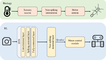
Figure 1: The correspondence diagram between our method and the sensory motor neuron pathway.

Inspired by neurobiology, Spiking Neural Networks (SNNs) use discrete events (spikes) to transmit information. Since SNNs have similar characteristics to biological neurons in the brain, they are regarded as the third generation of neural network models maass1997networks . In recent years, SNNs have attracted great research interest and have made rapid development in image classification tasks fang2021incorporating ; fang2021deep and robot control tasks mahadevuni2017navigating . Compared with Artificial Neural Networks (ANNs), SNNs have high biological plausibility and could greatly reduce the energy consumption on the special neuromorphic hardware.

An accumulating body of research studies shows that SNN can be used as energy-efficient solutions for robot control tasks with limited on-board energy resources mahadevuni2017navigating . To overcome the limitations of SNN in solving high-dimensional control problems, it would be natural to combine the energy-efficiency of SNN with the optimality of deep RL, which has been proved effective in extensive control tasks mnih2015human . Since rewards are regarded as the training guidance in RL, several works fremaux2013reinforcement employ reward-based learning using three-factor learning rules. However, these methods only apply to shallow SNNs and low-dimensional control tasks, or need to tune numerous hyper-parameters for each scenario bellec2020solution . Besides, several methods aim to apply the surrogate gradient method lee2016training to train SNN in RL. Since SNN usually uses the firing rate as the equivalent activation value rueckauer2017conversion which is a discrete value between 0 and 1, it is hard to represent the value function of RL which doesn’t have a certain range in training. Therefore, several methods patel2019improved ; tan2020strategy aim to convert the trained DQN to SNN for execution. In addition, several methods based on hybrid framework tang2020deep ; zhang2021population utilize SNN to model policy function (i.e., a probability distribution), and resort ANN to estimate value function for auxiliary training. However, these methods may lose the potential biological plausibility of SNN, and limit the application of different types of RL algorithm. In addition, RL needs a large number of trials in training, and the utilization of ANN may cause more energy consumption.

To handle these challenges, it is necessary to develop a spike-based RL method where only SNN is used in both training and execution. The key issue is to design a new neural coding method to decode the spike-train into the results of value function, realizing end-to-end spike-based RL. In nature, sensory neurons receive information from the external environment and transmit it to non-spiking interneurons through action potentials bidaye2018six , and then change the membrane voltage of motor neurons through graded signals, so as to achieve effective locomotion. As a translational unit, non-spiking interneurons could affect the motor output according to the sensory input.

Inspired by biological researches on sensorimotor neuron path, we propose a novel method to train SNN with deep Q-learning mnih2015human , where the membrane voltage of non-spiking neurons is used to represent the Q-value (i.e., the state-action value). As shown in Figure 1, SNN receives the state from the environment and encodes them as spike-train by spiking neurons. Then, the non-spiking neurons are subsequently introduced to calculate the membrane voltage from the spike-train, which is further used to predict the Q-value of each action. Finally, the agent selects the action with the maximum Q-value. To take full advantage of the membrane voltage in all simulation time and make the learning stable, we argue that the statistics of membrane voltage rather than the last membrane voltage should be used to represent Q-value. We empirically find that the maximum membrane voltage among all the simulation time can significantly enhance spike-based RL and ensure strong robustness. The main contributions of this paper is summarized as follows:

1. A novel spike-based RL method, referred to as deep spiking Q-network (DSQN), is proposed, which could represent Q-value by the membrane voltage of non-spiking neurons.

2. The method achieves end-to-end Q-learning without any additional ANN for auxiliary training, and maintains the high biological plausibility of SNN.

3. The method is evaluated on 17 Atari games, and our results outperform ANN-based DQN on most of the games. Moreover, the experimental results show superior learning stability and robustness to adversarial attacks such as FGSM goodfellow2014explaining .

2 Related Work

2.1 Reward-based Learning by Three-factor Learning Rules

To bridge the gap between the time scales of behavior and neuronal action potential, modern theories of synaptic plasticity assume that the co-activation of presynaptic and postsynaptic neurons sets a flag at the synapse, called eligibility trace sutton2018reinforcement . Only if a third factor, signaling reward, punishment, surprise or novelty, exists while the flag is set, the synaptic weight will change. Although the theoretical framework of three-factor learning rules has been developed in the past few decades, experimental evidence supporting eligibility trace has only been collected in the past few years. Through the derivation of the RL rule for continuous time, the existing approaches have been able to solve the standard control tasks fremaux2013reinforcement and robot control tasks mahadevuni2017navigating . However, these methods are only suitable for shallow SNNs and low-dimensional control tasks. To solve these problems, Bellec et al. bellec2020solution propose a learning method for recurrently connected networks of spiking neurons, which is called e-prop. Despite the agent learned by reward-based e-prop successfully wins Atari games, the need that numerous hyper-parameters should be adjusted between different tasks limits the application of this method.

2.2 ANN to SNN Conversion for RL

By matching the firing rates of spiking neurons with the graded activation of analog neurons, trained ANNs can be converted into corresponding SNNs with few accuracy loss rueckauer2017conversion . For the SNNs converted from the ANNs trained by DQN algorithm, the firing rate of spiking neurons in the output layer is proportional to the Q-value of the corresponding action, which makes it possible to select actions according to the relative size of the Q-value patel2019improved ; tan2020strategy . But there is a trade-off between the accuracy and the efficiency, which tells us that longer inference latency is needed to improve accuracy. As far as we know, for RL tasks, the converted SNNs cannot achieve better results than ANNs.

2.3 Co-learning of Hybrid Framework

Tang et al. tang2020reinforcement first propose the hybrid framework, composed of a spiking actor network (SAN) and a deep critic network. Through the co-learning of the two networks, these methods  tang2020deep ; zhang2021population avoid the problem of value estimation using SNNs. Hence, these methods only work for actor-critic structure, and the energy consumption in the training process is much higher than the pure SNN methods kim2021chip .

2.4 Non-spiking Neurons in Spike-based BP

Following the surrogate gradient method lee2016training , the spike-based backpropagation (BP) algorithm has quickly become the mainstream solution for training multi-layer SNNs fang2021incorporating ; fang2021deep . As shown in several open-source frameworks of SNNs SpikingJelly ; norse2021 , the membrane voltage of non-spiking neurons is feasible to represent a continuous value in a spike-based BP method. However, how to use it to effectively train SNN with Q-learning has not been systematically studied and remains unsolved, which is the goal of this paper.

3 Method

In this section, we present the deep spiking Q-network (DSQN) in detail. Firstly, we introduce the preliminary of RL, and the spiking neural model and its discrete dynamics are presented subsequently. Then, we propose the non-spiking neurons for DSQN and analyze the neural coding method. Finally, we present the learning algorithm of spike-based RL and derive the detailed learning rule.

3.1 Deep Q-learning

The goal of RL algorithm is to train a strategy to maximize the expected cumulative reward in a Markov decision process (MDP). In RL tasks, the agent interacts with the environment through a series of observations ($s$), actions ($a$) and rewards ($r$). The Q-value function $Q(s,a)$ is to estimate the expected cumulative rewards of performing action $a$ at $s$. We refer to a neural network function approximator with weights $\theta$ as the Q-network, which can be learned by minimizing the mean-squared error in the Bellman equation during the training process. Therefore, the loss function is defined as follows:

$$L\left(\theta\right)= \mathbb{E}_{s,a,r}\left[\left(\mathbb{E}_{s^{\prime}}\left[y\middle|s,a\right]-Q\left(s,a;\theta\right)\right)^{2}\right]$$

$$= \mathbb{E}_{s,a,r,s^{\prime}}\left[\left(y-Q\left(s,a;\theta\right)\right)^{2}\right]+\mathbb{E}_{s,a,r}\left[\mathbb{V}_{s^{\prime}}\left[y\right]\right],$$ (1)

where $y=r+\gamma\max\limits_{a^{\prime}}Q(s^{\prime},a^{\prime};\theta^{-})$. $s^{\prime}$ and $a^{\prime}$ represent the observation and the action at the next time-step, $\gamma$ is a discount factor and $\theta^{-}$ are the weights of the target network. $\mathbb{E}$ and $\mathbb{V}$ represent the expectation and the variance. More details of Eq. (3.1) refer to DQN mnih2015human . Differentiating the loss function with respect to the weights, we obtain the following gradient:

$$\nabla_{\theta}L\left(\theta\right)=\mathbb{E}_{s,a,r,s^{\prime}}\left[\left(y-Q\left(s,a;\theta\right)\right)\nabla_{\theta}Q\left(s,a;\theta\right)\right].$$ (2)

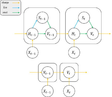
Figure 2: The general discrete neural model (Top) Spiking neural model. (Bottom) Non-spiking neural model.

3.2 Spiking Neural Model

The basic computing unit of SNN is the spiking neuron. The dynamics of all kinds of spiking neurons can be described as:

$$H_{t} =f\left(V_{t-1},X_{t}\right),$$ (3)

$$S_{t} =\mathrm{\Theta}\left(H_{t}-V_{th}\right),$$ (4)

$$V_{t} =H_{t}\left(1\ -\ S_{t}\right)+V_{reset}S_{t},$$ (5)

where $H_{t}$ and $V_{t}$ denote the membrane voltage after neural dynamics and the trigger of a spike at time-step $t$, respectively. $X_{t}$ denotes the external input, and $S_{t}$ means the output spike at time-step $t$, which equals 1 if there is a spike and 0 otherwise. $V_{th}$ denotes the threshold voltage and $V_{reset}$ denotes the membrane rest voltage. As shown in Figure 2, Eq. (3) - (5) establish a general mathematical model to describe the discrete dynamics of spiking neurons, which include charging, firing and resetting. Specifically, Eq. (3) describes the subthreshold dynamics, which vary with the type of neuron models. Here we consider the Leaky Integrate-and-Fire (LIF) model gerstner2014neuronal , which is one of the most common spiking neuron models used in SNNs. The function $f(\cdot)$ of the LIF neuron is defined as:

$$f\left(V_{t-1},X_{t}\right)=V_{t-1}+\frac{1}{\tau}\left(-\left(V_{t-1}-V_{reset}\right)+X_{t}\right),$$ (6)

where $\tau$ is the membrane time constant. The spike generative function $\Theta(x)$ is the Heaviside step function, which is defined by $\Theta(x)=1$ for $x\geq 0$ and $\Theta(x)=0$ for $x<0$. Note that $V_{0}=V_{reset}$.

3.3 Non-spiking Neural Model

Non-spiking neurons can be regarded as a special case of spiking neurons. If we set the threshold voltage $V_{th}$ of spiking neurons to infinity, the dynamics of neurons will always be under the threshold, which is so-called non-spiking neurons. Since non-spiking neurons do not have the dynamics of firing and resetting, we could simplify the neural model to the following equation (see Figure 2):

$$V_{t}=f\left(V_{t-1},X_{t}\right).$$ (7)

Here we consider the non-spiking LIF model, which can also be called Leaky Integrate (LI) model. The dynamics of LI neurons is described as the following equation:

$$V_{t}=V_{t-1}+\frac{1}{\tau}\left(-\left(V_{t-1}-V_{reset}\right)+X_{t}\right).$$ (8)

3.4 Neural Coding

According to the definition of SNN, the output is a spike-train, but the results of value estimation used in RL are continuous values. To bridge the difference between these two data forms, we need a spike decoder to complete the data conversion, that is non-spiking neurons. In the sensorimotor neuron path, the membrane voltage of non-spiking interneurons determines the input current of motor neurons. Therefore, for different non-spiking neurons, the greater the membrane voltage, the greater the probability of taking the corresponding action, which reminds us of the Q-value function in RL.

In the whole simulation time $T$, the non-spiking neurons take the spike-train as the input sequence, and then the membrane voltage $V_{t}$ at each time-step $t$ can be obtained. To represent the output of value function, we need to choose an optimal statistic according to the membrane voltage at all times.

To meet the needs of the algorithm, we finally design three statistics as candidates:

• Last membrane voltage (last-mem): It is a natural idea to use the last membrane voltage after the simulation time as the characterization of the Q-value ($Q=V_{T}$).

• Maximum membrane voltage (max-mem): By recording the membrane voltage of non-spiking neurons at each time-step in the whole simulation time, we can get the maximum membrane voltage ($Q=\max_{1\leq t\leq T}{V_{t}}$).

• Mean membrane voltage (mean-mem): Similar to the maximum membrane voltage, we can obtain the mean value by collecting the membrane voltage data, which is also a meaningful statistic ($Q=\frac{1}{T}\sum_{t=1}^{T}V_{t}$).

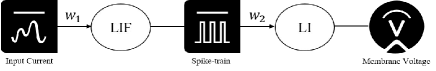
Figure 3: The architecture of the simple network for the case study on different statistics.

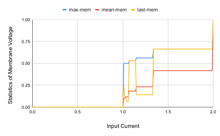
Figure 4: The functional relationship between the input current and the statistics of membrane voltage.

To have an intuitive understanding of the neuronal dynamics of non-spiking neurons decoded with different statistics, we conduct a case study to choose the decoder used in our methods. As illustrated in Figure 3, we consider a simple network as an example, which consists of a LIF neuron and a LI neuron. The LIF neuron receives the weighted input $X(t)=w_{1}I(t)$, and then transmits the weighted spike signal $w_{2}S(t)$ to the LI neuron. In this case, the input $I(t)$ is constant, and the simulation time $T$ is set to 8. Furthermore, the membrane rest voltage $V_{reset}$ is set to 0, and the membrane time constant $\tau$ is set to 2.0. For simplification, the weights $w_{1}$ and $w_{2}$ are set to 1.0. In Figure 4, we plot the functional relationship between the input current and different statistics of membrane voltage.

As we can see, due to the slight increase of input current, sometimes the firing time of LIF neurons will be advanced without generating more spikes, which leads to further attenuation of the membrane voltage caused by the spikes from the previous layer. So the membrane voltage of LI neurons at the last moment may be much lower, although the input current increases, which is not in line with our expectations. For max-mem and mean-mem, we empirically evaluate them in experiments respectively in Section 4.2.1, and the results are shown in Table. 1. We find both of them are effective and the max-mem performs better. Hence, we choose max-mem as the decoding method in the following sections.

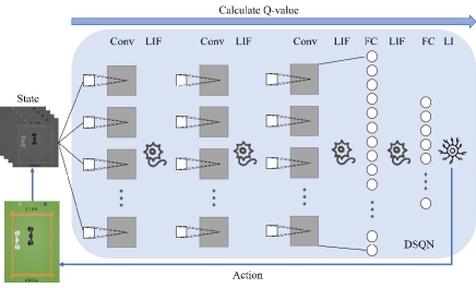
Figure 5: The architecture of deep spiking Q-network.

3.5 Deep Spiking Q-network

The typical architecture of DSQN is shown in Figure 5, which consists of synaptic layers and neuronal layers. The synaptic layers include convolutional layers and fully-connected (FC) layers, each of which is followed by a neuronal layer. Except that the LI layer is used after the last FC layer, the other synaptic layers are followed by LIF layers. In DSQN, all bias parameters are omitted and all weight parameters are shared at all simulation time-steps.

Note that we treat the synaptic layer and its subsequent neuronal layer as one layer in formula derivation. The former plays a similar role to dendrites in neuronal cells, and the latter works like the bodies and axons. Therefore, the first layer acts as a learnable spike encoder to convert the static state into the corresponding spike-train. During the task, the agent selects the action according to the Q-value calculated by the network in the simulation time, and then obtains the new environmental state to make the next decision.

3.6 Training Framework

Here we derive the detailed backpropagation training algorithm for DSQN. According to Eq. (2), we just need to derive the gradient of Q-value with respect to the weights using the network formula. Suppose that $\theta^{i}$ represents the weight parameter of the i-th layer in the network ($1\leq i\leq l$). For i-th layer, $I_{t}^{i}$ and $S_{t}^{i}$ represent the input and output signal at time-step $t$, which ensure that $I_{t}^{i}=S_{t}^{i-1}$ if $i>1$. The external input of neuronal model is $X_{t}^{i}=\theta^{i}I_{t}^{i}$. $\Theta^{\prime}(x)$ is defined by the surrogate function $\Theta^{\prime}(x)=\sigma^{\prime}(x)$. Taking the DSQN algorithm (max-mem) as an example, we can calculate the gradients recursively:

$$t^{\prime}=\mathop{\arg\max}\limits_{1\leq t\leq T}{V_{t}^{l}},$$ (9)

$$\frac{\delta V_{t}^{l}}{\delta\theta^{l}}=\left\{\begin{matrix}\frac{\delta V_{t}^{l}}{\delta V_{t-1}^{l}}\frac{\delta V_{t-1}^{l}}{\delta\theta^{l}}+\frac{\delta V_{t}^{l}}{\delta X_{t}^{l}}\frac{\delta X_{t}^{l}}{\delta\theta^{l}}&if\ t>1\\ \frac{\delta V_{t}^{l}}{\delta X_{t}^{l}}\frac{\delta X_{t}^{l}}{\delta\theta^{l}}&if\ t=1\\ \end{matrix}\right..$$ (10)

According to Eq. (3) - (5), we can get:

$$\frac{\delta Q}{\delta H_{t}^{i}}=\left\{\begin{matrix}\frac{\delta Q}{\delta H_{t+1}^{i}}\frac{\delta H_{t+1}^{i}}{\delta H_{t}^{i}}+\frac{\delta V_{t^{\prime}}^{l}}{\delta S_{t}^{l-1}}\frac{\delta S_{t}^{l-1}}{\delta H_{t}^{i}}&if\ t<t^{\prime}\\ \frac{\delta V_{t}^{l}}{\delta S_{t}^{l-1}}\frac{\delta S_{t}^{l-1}}{\delta H_{t}^{i}}&if\ t=t^{\prime}\\ 0&if\ t>t^{\prime}\\ \end{matrix}\right.,$$ (11)

$$\frac{\delta H_{t+1}^{i}}{\delta H_{t}^{i}}=\frac{\delta H_{t+1}^{i}}{\delta V_{t}^{i}}\frac{\delta V_{t}^{i}}{\delta H_{t}^{i}}=\left(1-\frac{1}{\tau}\right)\frac{\delta V_{t}^{i}}{\delta H_{t}^{i}},$$ (12)

$$\frac{\delta V_{t^{\prime}}^{l}}{\delta S_{t}^{l-1}}=\frac{\delta V_{t^{\prime}}^{l}}{\delta V_{t}^{l}}\frac{\delta V_{t}^{l}}{\delta X_{t}^{l}}\frac{\delta X_{t}^{l}}{\delta S_{t}^{l-1}}=\left(1-\frac{1}{\tau}\right)^{t^{\prime}-t}\frac{\theta^{l}}{\tau},$$ (13)

$$\frac{\delta S_{t}^{j}}{\delta H_{t}^{i}}=\left\{\begin{matrix}\frac{\delta S_{t}^{j}}{\delta H_{t}^{j}}\frac{\delta H_{t}^{j}}{\delta X_{t}^{j}}\frac{\delta X_{t}^{j}}{\delta S_{t}^{j-1}}\frac{\delta S_{t}^{j-1}}{\delta H_{t}^{i}}&if\ j>i\\ \sigma^{\prime}(H_{t}^{j}-V_{th})&if\ j=i\\ \end{matrix}\right.,$$ (14)

$$\frac{\delta V_{t}^{i}}{\delta H_{t}^{i}}=1-S_{t}^{i}+\left(V_{reset}-H_{t}^{i}\right)\frac{\delta S_{t}^{i}}{\delta H_{t}^{i}},$$ (15)

$$\frac{\delta H_{t}^{i}}{\delta\theta^{i}}=\left\{\begin{matrix}\frac{\delta H_{t}^{i}}{\delta V_{t-1}^{i}}\frac{\delta V_{t-1}^{i}}{\delta H_{t-1}^{i}}\frac{\delta H_{t-1}^{i}}{\delta\theta^{i}}+\frac{\delta H_{t}^{i}}{\delta X_{t}^{i}}\frac{\delta X_{t}^{i}}{\delta\theta^{i}}&if\ t>1\\ \frac{\delta H_{t}^{i}}{\delta X_{t}^{i}}\frac{\delta X_{t}^{i}}{\delta\theta^{i}}&if\ t=1\\ \end{matrix}\right..$$ (16)

Finally, we can get the gradients of the weight parameters:

$$\frac{\delta Q}{\delta\theta^{i}}=\left\{\begin{matrix}\sum_{t=1}^{T}{\frac{\delta Q}{\delta H_{t}^{i}}\frac{\delta H_{t}^{i}}{\delta\theta^{i}}}&i<l\\ \frac{\delta V_{t^{\prime}}^{i}}{\delta\theta^{i}}&i=l\\ \end{matrix}\right..$$ (17)

The gradient of mean-mem based DSQN could be derived in a similar way.

4 Experiments

In this section, we firstly compare the different decoders to choose, and evaluate the performance of DSQN on 17 Atari 2600 games from the arcade learning environment (ALE) bellemare2013arcade . Furthermore, we experimentally evaluate the robustness of DSQN when dealing with adversarial attacks. Our implementation of DSQN is based on the open-source framework of SNN SpikingJelly .

4.1 Experimental Settings

For Atari games, the ANN used in DQN mnih2015human contains 3 convolutional layers and 2 FC layers (i.e., Input-32C8S4-ReLU-64C4S2-ReLU-64C3S1-ReLU-Flatten-512-ReLU-$N_{A}$, where $N_{A}$ is the number of actions used in the task). For a fair comparison, DSQN employs a similar network structure for fair comparison (i.e., Input-32C8S4-LIF-64C4S2-LIF-64C3S1-LIF-Flatten-512-LIF-$N_{A}$-LI). The arctangent function is used as the surrogate function. The gradient is defined by

$$\sigma^{\prime}(x)=\frac{1}{1+(\pi x)^{2}},$$ (18)

where the primitive function is

$$\sigma(x)=\frac{1}{\pi}\arctan{\pi x}+\frac{1}{2}.$$ (19)

Due to the limitation of resources, we choose 17 top-performing Atari games selected by tan2020strategy to test the method. The network architecture and hyper-parameters keep identical across all 17 games. The hyper-parameters are same with mnih2015human , except that we use the Adam optimizer with the learning rate 0.00025 and train for a total of 20 million frames. This change is to improve the training efficiency of the tasks on the premise of ensuring high performance. Detailed tables of hyper-parameters are listed in the supplementary.

4.2 Performance

To obtain the optimal performance of each method, we evaluate the model every 100,000 frames during the training process, with a total of 30 episodes of each test. During the evaluation, the agent starts with a random number (up to 30 times) of no-op actions in each episode, and the behavior policy is $\epsilon$-greedy with $\epsilon$ fixed at 0.05. Due to space constraints, here we only report the optimal performance of different models and several typical learning curves. The complete learning curves are shown in the supplementary as well as the raw and normalized scores.

Game	max-mem	mean-mem
Atlantis	2481620.0	2394466.7
Beam Rider	5188.9	4917.3
Boxing	84.4	57.4
Breakout	360.8	340.3

Table 1: The mean scores of Atari games obtained by DSQN with different decoders. The simulation time $T$ is set to 8.

Game	DQN	ANN-SNN	DSQN
Atlantis	2945880.0	1880009.1	2481620.0
Beam Rider	5211.5	3938.8	5188.9
Boxing	28.3	22.4	84.4
Breakout	249.9	179.6	360.8
Crazy Climber	85396.7	71370.0	93753.3
Gopher	2788.7	1509.3	4154.0
Jamesbond	406.7	228.3	463.3
Kangaroo	6493.3	6013.3	6140.0
Krull	24042.9	16501.8	6899.0
Name This Game	4647.0	4359.3	7082.7
Pong	-20.5	-20.7	19.1
Road Runner	2530.0	620.0	23206.7
Space Invaders	1059.7	994.0	1132.3
Star Gunner	1116.7	1046.7	1716.7
Tennis	-1.0	-1.0	-1.0
Tutankham	98.4	75.4	276.0
Video Pinball	276040.2	28940.2	441615.2

Table 2: The mean scores of Atari games obtained by DQN , Converted SNN (ANN-SNN) and DSQN. The simulation time $T$ is set to 500 (ANN-SNN) and 8 (DSQN), respectively.

4.2.1 Analysis of Decoders

We compare the performance of DSQN with different decoders on four games selected in alphabetical order (Table 1). In all of these games, the DSQN with the maximum membrane voltage achieves better performance. Hence we use the maximum membrane voltage in the subsequent experiments.

	DQN			DSQN
Game	before	after	decay rate	before	after	decay rate
Atlantis	2945880.0	22543.3	99.23%	2481620.0	34666.7	98.60%
Beam Rider	5211.5	2055.0	60.57%	5188.9	4198.0	19.10%
Boxing	28.3	15.4	45.70%	84.4	77.5	8.14%
Breakout	249.9	1.2	99.53%	360.8	19.3	94.65%
Crazy Climber	85396.7	19390.0	77.29%	93753.3	82933.3	11.54%
Gopher	2788.7	580.7	79.18%	4154.0	1780.5	57.14%
Jamesbond	406.7	201.7	50.41%	463.3	350.0	24.46%
Kangaroo	6493.3	1293.3	80.08%	6140.0	1754.5	71.43%
Krull	24042.9	21204.0	11.81%	6899.0	6528.3	5.37%
Name This Game	4647.0	1796.3	61.34%	7082.7	6367.7	10.10%
Pong	-20.5	-20.7	-	19.1	4.8	74.87%
Road Runner	2530.0	2023.3	20.03%	23206.7	20666.7	10.94%
Space Invaders	1059.7	540.2	49.02%	1132.3	915.0	19.19%
Star Gunner	1116.7	1013.3	9.25%	1716.7	1713.9	0.16%
Tennis	-1.0	-2.7	-	-1.0	-1.2	-
Tutankham	98.4	15.6	84.17%	276.0	116.0	57.97%
Video Pinball	276040.2	43437.2	84.26%	441615.2	441592.7	0.01%

Table 3: The mean scores of DQN and DSQN when dealing with adversarial attacks. Since the decay rate cannot be used for comparison when the reward is negative, some values are omitted.

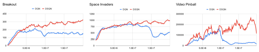
Figure 6: Learning curves of DQN and DSQN. Each curve is smoothed with a moving average of 10 to improve readability.

4.2.2 The Performance of DSQNs on Atari Games

The DSQN is compared with DQN and Converted SNN (ANN-SNN) tan2020strategy , where DQN and ANN-SNN are re-run under the same experimental setting for a fair comparison. As shown in Table 2, DSQN achieves better or comparable performance with DQN on most games. In addition, the learning of DSQN is more stable and could handle over-estimation well on most games, as shown in Figure 6 (see the supplementary for the learning curves of all Atari games). It indicates DSQN could control an agent effectively, and provides a promising way to the energy-efficient control tasks. In addition, DSQN also outperforms ANN-SNN on most games using fewer simulation time-steps $T$. The reason is that ANN-SNN is limited by the trained ANN, while DSQN is trained directly from the environment.

4.3 Robustness to White-box Attacks

Previous study patel2019improved shows that SNN could improve robustness to occlusion in the input image. To verify the robustness of DSQN, DSQN and DQN are evaluated under the white-box attacks respectively. Due to the large number of frames used in RL tasks, the Fast Gradient Sign Method (FGSM) goodfellow2014explaining is used to generate adversarial examples efficiently. Given a Q-network with parameters $\theta$ and loss $L(\theta,x,y)$, where $x$ is the input state and $y$ is a softmax of the computed Q-values, using FGSM results in a perturbation of

$$\eta=\epsilon\,sign\left(\nabla_{x}L(\theta,x,y)\right).$$ (20)

We change the strategy of the Q-network to deterministic, and the goal of the white-box attack is to make agents change the action selection by generating adversarial perturbations iteratively. The iteration is set to 50 at most.

Table 3 shows the performances of DQN and DSQN when dealing with adversarial attacks, where the decay rate represents the percentage of decline in the score of an agent after encountering adversarial attacks. Experimental results demonstrate the superior robustness of the proposed DSQN.

5 Conclusion

This paper presents a novel deep spiking Q-network to train SNN in RL task, by directly representing the Q-value with the maximum membrane voltage of non-spiking neurons. The method is evaluated on 17 Atari games, and outperforms ANN-based DQN in most scenarios. In addition, the experimental results indicate the robustness of the method under white-box attacks. The biological plausibility and theoretical proof will be explored in the future. We hope that this work can pave the way for the SNN-based RL.

References

- [1] Guillaume Bellec, Franz Scherr, Anand Subramoney, Elias Hajek, Darjan Salaj, Robert Legenstein, and Wolfgang Maass. A solution to the learning dilemma for recurrent networks of spiking neurons. Nature communications, 11(1):1–15, 2020.
- [2] Marc G Bellemare, Yavar Naddaf, Joel Veness, and Michael Bowling. The arcade learning environment: An evaluation platform for general agents. Journal of Artificial Intelligence Research, 47:253–279, 2013.
- [3] Salil S Bidaye, Till Bockemühl, and Ansgar Büschges. Six-legged walking in insects: how cpgs, peripheral feedback, and descending signals generate coordinated and adaptive motor rhythms. Journal of neurophysiology, 119(2):459–475, 2018.
- [4] Wei Fang, Yanqi Chen, Jianhao Ding, Ding Chen, Zhaofei Yu, Huihui Zhou, Yonghong Tian, and other contributors. Spikingjelly. https://github.com/fangwei123456/spikingjelly, 2020. Accessed: 2021-12-01.
- [5] Wei Fang, Zhaofei Yu, Yanqi Chen, Tiejun Huang, Timothée Masquelier, and Yonghong Tian. Deep residual learning in spiking neural networks. In Thirty-Fifth Conference on Neural Information Processing Systems, 2021.
- [6] Wei Fang, Zhaofei Yu, Yanqi Chen, Timothee Masquelier, Tiejun Huang, and Yonghong Tian. Incorporating learnable membrane time constant to enhance learning of spiking neural networks. In Proceedings of the IEEE/CVF International Conference on Computer Vision, pages 2661–2671, 2021.
- [7] Nicolas Frémaux, Henning Sprekeler, and Wulfram Gerstner. Reinforcement learning using a continuous time actor-critic framework with spiking neurons. PLoS computational biology, 9(4):e1003024, 2013.
- [8] Wulfram Gerstner, Werner M Kistler, Richard Naud, and Liam Paninski. Neuronal dynamics: From single neurons to networks and models of cognition. Cambridge University Press, 2014.
- [9] Ian J Goodfellow, Jonathon Shlens, and Christian Szegedy. Explaining and harnessing adversarial examples. arXiv preprint arXiv:1412.6572, 2014.
- [10] Jangsaeng Kim, Dongseok Kwon, Sung Yun Woo, Won-Mook Kang, Soochang Lee, Seongbin Oh, Chul-Heung Kim, Jong-Ho Bae, Byung-Gook Park, and Jong-Ho Lee. On-chip trainable hardware-based deep q-networks approximating a backpropagation algorithm. Neural Computing and Applications, pages 1–12, 2021.
- [11] Jun Haeng Lee, Tobi Delbruck, and Michael Pfeiffer. Training deep spiking neural networks using backpropagation. Frontiers in neuroscience, 10:508, 2016.
- [12] Wolfgang Maass. Networks of spiking neurons: the third generation of neural network models. Neural networks, 10(9):1659–1671, 1997.
- [13] Amarnath Mahadevuni and Peng Li. Navigating mobile robots to target in near shortest time using reinforcement learning with spiking neural networks. In 2017 International Joint Conference on Neural Networks (IJCNN), pages 2243–2250. IEEE, 2017.
- [14] Volodymyr Mnih, Koray Kavukcuoglu, David Silver, Andrei A Rusu, Joel Veness, Marc G Bellemare, Alex Graves, Martin Riedmiller, Andreas K Fidjeland, Georg Ostrovski, et al. Human-level control through deep reinforcement learning. nature, 518(7540):529–533, 2015.
- [15] Devdhar Patel, Hananel Hazan, Daniel J Saunders, Hava T Siegelmann, and Robert Kozma. Improved robustness of reinforcement learning policies upon conversion to spiking neuronal network platforms applied to atari breakout game. Neural Networks, 120:108–115, 2019.
- [16] Christian Pehle and Jens Egholm Pedersen. Norse - a deep learning library for spiking neural networks, January 2021. Documentation: https://norse.ai/docs/.
- [17] Bodo Rueckauer, Iulia-Alexandra Lungu, Yuhuang Hu, Michael Pfeiffer, and Shih-Chii Liu. Conversion of continuous-valued deep networks to efficient event-driven networks for image classification. Frontiers in neuroscience, 11:682, 2017.
- [18] Richard S Sutton and Andrew G Barto. Reinforcement learning: An introduction. MIT press, 2018.
- [19] Weihao Tan, Devdhar Patel, and Robert Kozma. Strategy and benchmark for converting deep q-networks to event-driven spiking neural networks. arXiv preprint arXiv:2009.14456, 2020.
- [20] Guangzhi Tang, Neelesh Kumar, and Konstantinos P Michmizos. Reinforcement co-learning of deep and spiking neural networks for energy-efficient mapless navigation with neuromorphic hardware. In 2020 IEEE/RSJ International Conference on Intelligent Robots and Systems (IROS), pages 6090–6097. IEEE, 2020.
- [21] Guangzhi Tang, Neelesh Kumar, Raymond Yoo, and Konstantinos P Michmizos. Deep reinforcement learning with population-coded spiking neural network for continuous control. arXiv preprint arXiv:2010.09635, 2020.
- [22] Duzhen Zhang, Tielin Zhang, Shuncheng Jia, Xiang Cheng, and Bo Xu. Population-coding and dynamic-neurons improved spiking actor network for reinforcement learning. arXiv preprint arXiv:2106.07854, 2021.