Disorder-induced dynamical Griffiths singularities after certain quantum quenches

Abstract

We demonstrate that in a class of disordered quantum systems the dynamical partition function is not an analytical function in a time window after certain quantum quenches. We related this behavior to rare and large regions with atypical inhomogeneity configurations. We also quantify the strength of the associated singularities and their signatures in experiments and numerical studies.

Published in Phys. Rev. B 106, L140201 (2022); DOI: 10.1103/PhysRevB.106.L140201

Phase transitions (PTs) are among the most intriguing phenomena in nature. When crossed, the macroscopic properties of matter change fundamentally, often requiring new concepts for a proper description (Fisher, 1965). In thermodynamic equilibrium, PTs are on firm theoretical grounds as they occur whenever a zero of the partition function touches the real-temperature (or field) axis (Yang and Lee, 1952; Fisher, 1965). Consequently, thermodynamic observables become non-analytic functions of temperature/field at the transition point. Notably, these Yang-Lee-Fisher (YLF) zeros were recently measured experimentally (Peng et al., 2015; Brandner et al., 2017).

Inhomogeneities, which are nearly ubiquitous in experiments, play an important role in equilibrium PTs. For instance, even the smallest amount of them can change the singularities of a critical system (Harris, 1974), smear the PT (Vojta, 2003; Hoyos and Vojta, 2008), or even destroy it (Imry and Ma, 1975). Another remarkable inhomogeneity-induced phenomenon is the stabilization of a Griffiths phase (GP): an extended region in the phase diagram surrounding a phase-transition manifold where the free energy is non-analytic (Griffiths, 1969; McCoy, 1969). Counterintuitively, the non-analyticity is due to so-called rare regions (RRs)—large and rare regions in space with atypical configurations of inhomogeneities—which provide YLF zeros arbitrarily close to the real-temperature axis (Griffiths, 1969; Wortis, 1974; Harris, 1975).

Over the past decades, the influence of the RRs on many observables has been quantified in a multitude of strongly interacting systems ranging from classical and quantum models in equilibrium to non-equilibrium reaction-diffusion models (for reviews, see Refs. Iglói and Monthus, 2005; Vojta, 2006; Iglói and Monthus, 2018). In the associated GPs, the RRs endow many observables with singular behavior in the long-time/low-frequency regime. This common feature is due to the RRs’ long relaxation times (Randeria et al., 1985; Bray, 1987, 1988; Thill and Huse, 1995; Vojta and Hoyos, 2014).

With the growing capacity of experimentally accessing the time evolution of closed quantum many-body systems (Bloch et al., 2008; Georgescu et al., 2014), it then became natural to inquire whether the RRs play any important role in their time evolution. Clearly, the notion of slow RRs at equilibrium does not apply and thus their importance cannot be anticipated. Evidently, obtaining a result on the RR effects in a general out-of-equilibrium situation is desirable but very unlikely to exist. We thus restrict ourselves to the simpler case of quantum quenches which already allows the study of fundamental phenomena such as entanglement spreading and thermalization (Calabrese and Cardy, 2006; Polkovnikov et al., 2011; Mitra, 2018). Here, the system’s initial state is $\left|\psi_{0}\right\rangle$, the ground state of $H_{0}\equiv H\left(h_{0}\right)$, and time evolved according to the postquench Hamiltonian $H\equiv H\left(h\right)$, with $h$ being a tuning parameter. In this context, the concept of dynamical quantum phase transitions (QPTs) is quite useful (Heyl et al., 2013) because an analogy with equilibrium PTs can be made. The linking quantity is the dynamical free energy

$$f(t)=-V^{-1}\ln\left|Z(t)\right|^{2},\mbox{ where }Z(z)=\left\langle\psi_{0}\left|e^{-iHz}\right|\psi_{0}\right\rangle$$ (1)

is the return probability amplitude after the quench, $z=t+i\tau$ is the complex time, and $V$ is the system volume. $Z$ is the dynamical analog of the equilibrium partition function. As in equilibrium PTs, its zeros accumulate in lines or areas on the complex-time plane and, in the thermodynamic limit, may touch the real-time axis. When this happens, a dynamical QPT occurs (Heyl et al., 2013; Andraschko and Sirker, 2014; Vajna and Dóra, 2014; Schmitt and Kehrein, 2015; Halimeh and Zauner-Stauber, 2017; Žunkovič et al., 2018; Jafari, 2019) and has been experimentally verified in different quantum simulator platforms (Jurcevic et al., 2017; Zhang et al., 2017; Bernie et al., 2017; Fläschner et al., 2018; Guo et al., 2019) (for a review, see Ref. Heyl, 2018).

In this Letter, we use the unifying concept of YLF zeros to show that the RRs dominate the system’s early-time dynamics for all quenches which do not cross the bulk equilibrium QPT but do cross the RR local QPT, i.e., the quantum quenches are from a conventional phase to the nearby GP [see Fig. 1(a)]. For those quenches, the RRs endow $Z(z)$ with YLF zeros arbitrarily close to the real-time axis. As in equilibrium GPs, these YLF zeros are spread over an area on the complex-time plane with the associated density of zeros depending on the details of the disorder variables in $H$ [see Fig. 1(b)]. We thus propose the term dynamical quantum Griffiths phase to designate the real-time axis interval intersected by the YLF zeros [see Fig. 1(c)].

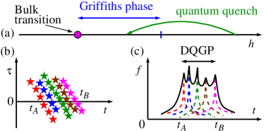
Figure 1: Schematics of (a) the equilibrium phase diagram and the class of quantum quenches studied: from a point far from the quantum phase transition to a point in the nearby Griffiths phase. (b) The rare-region-induced zeros of the dynamical partition function $Z$, and (c) the associated dynamical free energy $f$ (solid line). Each set of zeros (stars of a given color) and the corresponding dynamical free energy $f_{\text{RR}}$ (dashed line) are due to a single rare region. The singular part of $f$ is a simple superposition of all $f_{\text{RR}}$. The time window $t_{A}<t<t_{B}$ is the dynamical quantum Griffiths phase.

The reasoning behind our result is as follows. After the quench, the bulk remains nearly in its ground state since its QPT was not crossed. The RRs, however, are highly excited. Because the RRs and the bulk are in different phases, these excitations do not rapidly decay. Thus, meanwhile, the RRs’ dynamics is decoupled from the bulk’s in a sense that will become precise later. Consequently, two sets of YLF zeros appear, one provided by the bulk and the other by the RRs. Those from the bulk are far from the real-time axis and thus only provide analytical contributions to $f(t)$. Those from the RRs, however, are arbitrarily close to the real-time axis and therefore are responsible for the non-analyticities of $f(t)$. In addition, we show that this singular behavior can be well approximated by that of completely decoupled RRs with open boundary conditions undergoing the same quantum quench.

We remark that, differently from the known cases in the literature, the RRs in dynamical QPTs dominate the short-time dynamics. This is exciting because it allows for an easier identification of the RRs’ effects in numerical studies and in experiments.

Finally, we notice that quenched disorder effects on dynamical QPTs were studied in a variety of models (Obuchi and Takahashi, 2012; Yang et al., 2017; Yin et al., 2018; Gurarie, 2019; Cao et al., 2020; Mishra et al., 2020). These studies, however, did not focus on the RR-induced effects.

In the remainder of this Letter, we derive our results from an explicit model Hamiltonian, discuss their generality and extensions, and provide concluding remarks.

Consider the transverse-field Ising chain

$$H=-\sum_{i=1}^{L}J_{i}\sigma_{i}^{z}\sigma_{i+1}^{z}-h\sum_{i=1}^{L}\sigma_{i}^{x},$$ (2)

where $\boldsymbol{\sigma}_{i}$ are Pauli matrices, $J_{i}>0$ are the ferromagnetic coupling constants (which, due to inhomogeneities, are site dependent), and $h>0$ is the transverse field and plays the role of the tuning parameter of $H\left(h\right)$. We consider chains of $L$ sites long with periodic boundary conditions $\boldsymbol{\sigma}_{L+i}=\boldsymbol{\sigma}_{i}$. The model has two zero-temperature phases: the ferromagnet ($h<h_{c}$) and the paramagnet ($h>h_{c}$) separated by a quantum critical point at $h_{c}=J_{\text{typ}}$, where $J_{\text{typ}}=e^{\overline{\ln J}}$ is the geometric mean of the coupling constants (Pfeuty, 1979).

The clean system ($J_{i}=J$) can be solved analytically using standard methods (sup, ). The return probability amplitude (1) after the quantum quench $h_{0}\rightarrow h$ (with $h_{0}>h_{c})$ is

$$Z(z)=e^{-iE_{0}z}\prod_{0<k_{n}<\pi}\left(1-\frac{\left(1-\varepsilon_{k_{n}}\right)\left(1-e^{-4i\omega_{k_{n}}\left(h\right)z}\right)}{2}\right),$$ (3)

where $E_{0}=-\sum_{n=1}^{L}\omega_{k_{n}}\left(h\right)$ is the ground-state energy of the post-quench Hamiltonian, the momenta $k_{n}=\left(2n-1\right)\frac{\pi}{L},$ $n=1,\dots,L,$ $\omega_{k}\left(h\right)=\sqrt{h^{2}-2hJ\cos k+J^{2}}$ is the dispersion relation, and $\varepsilon_{k}=\varepsilon_{k}(h,h_{0})\equiv\left[hh_{0}-J\left(h_{0}+h\right)\cos k+J^{2}\right]/\left[\omega_{k}\left(h\right)\omega_{k}\left(h_{0}\right)\right]$. The YLF zeros of (3), $z^{*}=t^{*}+i\tau^{*}$, are

$$t_{m,n}^{*}=\frac{\left(2m+1\right)\pi}{4\omega_{k_{n}}\left(h\right)}\text{ and }\tau_{n}^{*}=\frac{\ln\left(\frac{1+\varepsilon_{k_{n}}(h,h_{0})}{1-\varepsilon_{k_{n}}(h,h_{0})}\right)}{4\omega_{k_{n}}\left(h\right)},$$ (4)

where $m\in\mathbb{N}$ defines different accumulation lines of zeros (for a graphical illustration, see (sup, )). These lines pierce the real-time axis if and only if the equilibrium QPT is crossed by the quantum quench, i.e., iff $\left(h-h_{c}\right)\left(h_{0}-h_{c}\right)<0$ in the model (2). In the following, we numerically demonstrate that even a single RR dramatically change this scenario.

Unfortunately, there is no analytical solution for the non-homogeneous case. We then compute $Z(z)$ in (1) via exact numerical diagonalization and find its YLF zeros $z^{*}$ using the standard secant method (sup, ). For definiteness, we set the couplings in the Hamiltonian (2) to $J_{i}=J_{\text{B}}$ (the bulk couplings) everywhere except inside a RR where $J_{i}=J_{\text{RR}}$ for $1\leq i\leq L_{\text{RR}}-1$. The fact that we are considering a compact RR is of no consequence for our purposes. Later, we discuss more general profiles. For simplicity, we consider quantum quenches from $h_{0}=\infty$ to a finite $h$. Thus, $\left|\psi_{0}\right\rangle=\otimes_{i=1}^{L}\left|\rightarrow\right\rangle$, with $\sigma^{x}\left|\rightarrow\right\rangle=\left|\rightarrow\right\rangle$, is a simple product state. We want to study quenches that do not cross the bulk QPT, and thus $h>J_{\text{B}}$. In the following numerical study, we set $h=5J_{\text{B}}$. Other values only produce quantitative changes and will be shown elsewhere.

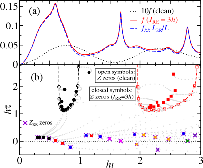
Figure 2: (a) The dynamical free energy $f$ as a function of the real time $t$ for three different chains after the quantum quench from $h_{0}=\infty$ to finite $h$. The first chain (black dotted line) is homogeneous, $L=30$ sites long with periodic boundary conditions, and has couplings $J_{\text{B}}=h/5$. The second chain (red solid line) is identical to the first one except that it contains a RR of size $L_{\text{RR}}=8$ inside which the couplings are $J_{\text{RR}}=3h$. The third chain (blue dashed line) is homogeneous, $L_{\text{RR}}$ sites long with open boundary conditions, and has couplings $J_{\text{RR}}$. (b) The corresponding Yang-Lee-Fisher zeros of $Z(z)$ for these three chains: open symbols, solid symbols, and $\times$ symbols, respectively. The zeros’ trajectories of the second chain (when changing $J_{\text{RR}}$ from $h/5$ to $3h$) are given by the gray dots (see text).

We show in Fig. 2(a) the dynamical free energy for the homogeneous case $J_{\text{RR}}=J_{\text{B}}$ for a chain of only $L=30$ sites long (for the sake of clarity) with periodic boundary conditions. The resulting curve (dotted line; notice it is multiplied by a factor of $10$) is completely smooth and analytic as expected. The corresponding YLF zeros Eq. (4) are shown in Fig. 2(b) as open symbols. As is well known (Heyl et al., 2013), they accumulate in lines far from the real-time axis. For the time window considered, only the first two accumulation (dashed) lines appear. Increasing $J_{\text{RR}}$ gradually (in steps of $0.1h$ up to $3h$ and considering, for the sake of clarity, a rare region of only $L_{\text{RR}}=8$ sites long), the zeros move on the complex-time plane [see gray dots in Fig. 2(b)]. Analyzing their trajectories, we verify two distinct sets of zeros: one that remains in the upper half of the complex-time plane and the other which migrates to the vicinity of the real-time axis. The latter set of zeros accumulate in lines which pierce the real-time axis for $J_{\text{RR}}>h$. For the case $J_{\text{RR}}=3h$, we plot the corresponding $f(t)$ in Fig. 2(a) (red solid line). The corresponding zeros are shown in Fig. 2(b) as solid symbols. The developing singularities in $f(t)$ are in one-to-one correspondence with the zeros close to the real-time axis.

Our interpretation of the latter set of zeros is that the unitary dynamics of the RR is essentially decoupled from the bulk. The reasoning is as follows. The bulk is gapful and is locally in a different phase from the RR. The RR excitations (kinks) have a different nature from the bulk’s (spin flips). Therefore, the quench-induced excitations of the RR do not immediately decay into the bulk.

To give support to this interpretation, we compute the dynamical free energy $f_{\text{RR}}$ and the corresponding YLF zeros of a decoupled RR with open boundary conditions undergoing the same quantum quench: the blue dashed line and violet $\times$ symbols in Figs. 2(a) and 2(b), respectively. We verify that $f_{\text{RR}}(t)$ accurately reproduces the singular part of $f(t)$, the difference being due to the analytical bulk’s contribution. Interestingly, we verify a one-to-one correspondence between the set of zeros of $Z(z)$ near the real-time axis and the zeros of $Z_{\text{RR}}(z)$. The differences between them vanish exponentially as $J_{\text{RR}}$ increases (sup, ).

We now further explore the consequences of our interpretation: (i) Different RRs are independent (if sufficiently far from each other) and (ii) the post-quench excitations are localized inside the RRs (for sufficiently short times). The reasoning behind (i) is because the bulk is practically in its ground state and thus its ground-state correlation length $\xi$ is still a well-defined quantity.

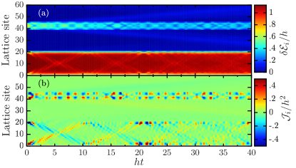
Figure 3: (a) The mean energy density above the ground state $\delta{\cal E}_{i}$ and (b) the corresponding density current ${\cal J}_{i}$ as a function of the real time $t$ for each lattice site $i$ (see text).

To give evidence of the above statements, we study the time evolution of the mean energy density above the ground state $\delta{\cal E}_{i}=\left\langle\psi\left(t\right)\left|E_{i}\right|\psi\left(t\right)\right\rangle-\left\langle\phi_{\text{GS}}\left|E_{i}\right|\phi_{\text{GS}}\right\rangle$ (where $E_{i}=-\frac{1}{2}J_{i-1}\sigma_{i-1}^{z}\sigma_{i}^{z}-h\sigma_{i}^{x}-\frac{1}{2}J_{i}\sigma_{i}^{z}\sigma_{i+1}^{z}$ and $\left|\phi_{\text{GS}}\right\rangle$ is the ground state of the post-quench $H$) and the associated density current ${\cal J}_{i}=hJ_{i-1}\left\langle\psi\left(t\right)\left|-\sigma_{i-1}^{z}\sigma_{i}^{y}+\sigma_{i-1}^{y}\sigma_{i}^{z}\right|\psi\left(t\right)\right\rangle$ (sup, ). We consider the same quench (from $h_{0}=\infty$ to $h$) in a chain of $L=60$ sites long with periodic boundary conditions where the bulk coupling is $J_{\text{B}}=0.2h$. The chain has two RRs. One is $20$ sites long with coupling constant $J_{\text{RR},1}=2h$, and the other is only $5$ sites long with couplings $J_{\text{RR},2}=1.5h$. In Fig. 3, we plot the $\delta{\cal E}_{i}$ and ${\cal J}_{i}$ as a function of time.

Clearly, for the time window studied, the excitations are well localized inside the RRs and the bulk remains in its ground state carrying no energy current. We have also verified (sup, ) that the singular part of $f(t)$ and the corresponding YLF zeros are well described by those of the same RRs undergoing the same quantum quench but decoupled from the bulk.

Having demonstrated that (i) the RR dynamics is effectively decoupled from the bulk and (ii) that the dynamics of sufficiently far apart RRs are essentially independent from each other, we can readily understand the origin and quantify the non-analyticities of $f(t)$ for any quantum quench which does not cross the bulk QPT. All the singularities come from sufficiently large RRs which, independently, provide YLF zeros accumulating in lines piercing the real-time axis. Since the time instant in which these lines pierce the real-time axis depends on the microscopic details of the RRs, the YLF zeros will be generically distributed over an area of the complex-time plane. The intersection of this area with the real-time axis defines the dynamical quantum Griffiths phase (see Fig. 1).

Evidently, besides identifying the physical mechanism behind the non-analyticities in $Z(t)$, it is also desirable to quantify it. From the Weierstrass factorization theorem, the singular part of $f(t)$ is (Yang and Lee, 1952; Fisher, 1965; Heyl, 2018)

$$f_{\text{sing}}(t)\propto\sum_{m,\alpha}\ln\left|t-t_{m,\alpha}^{*}\right|\rightarrow\int\text{d}t^{*}g(t^{*})\ln\left|t-t^{*}\right|.$$ (5)

Here, $t_{m,\alpha}^{*}$ is the $m$th real-time YLF zero due to the $\alpha$th RR. In the thermodynamic limit, the sum in Eq. (5) is replaced by an integral weighted by the distribution of zeros $g(t^{*})$. As noticed by Fisher (Fisher, 1965), $f_{\text{sing}}$ is as a two-dimensional electrostatic potential due to point charges at $t^{*}$. The non-analyticity of $f(t)$ is thus encoded in the distribution $g(t)$, whose non-analyticities are inherited from the distribution of the random variables in $H$. Naturally, an example that can be worked out analytically is desirable. This is provided by the percolating case in which the couplings are vanishing with probability $p$ and equal to $J_{\alpha}>0$ with probability $1-p$. Here, $J_{\alpha}$ is a random variable distributed according to $P(J)$. For the quantum quench $h_{0}=\infty\rightarrow h=0_{+}$, the dynamical free energy is (sup, )

$$f=-L^{-1}\sum_{k=1}^{L}\ln\cos^{2}\left(J_{k}t\right)\rightarrow-\left(1-p\right)\overline{\ln\cos^{2}\left(Jt\right)},$$ (6)

where the thermodynamic limit was taken in the last passage and $\overline{(\cdots)}=\int\text{d}JP(J)(\cdots)$. The real-time YLF zeros are $t_{m,\alpha}^{*}=\left(2m_{\alpha}+1\right)\pi/J_{\alpha}$. If $J_{\alpha}$ is uniformly distributed between $J_{1}$ and $J_{2}$, the non-analyticities of $P(J)$ at $J=J_{1(2)}$ become non-analyticities of $f(t)$ at the time instants $t_{m,1(2)}^{c}=\left(2m_{1(2)}+1\right)\pi/J_{1(2)}$. Notice that these are the only time instants in which $f(t)$ is non-analytic, even though there is a continuum of YLF zeros in the time window $t_{m,2}^{c}<t<t_{m,1}^{c}$. This is in close correspondence with the non-analyticities of the electrostatic potential due to a continuous distribution of charges. The associated singularities are only log-infinite derivatives of $f$ at the instants $t_{m,2}^{c}$ and $t_{m,1}^{c}$. At all other time instants, $f$ is locally analytic. At first glance, this seems to imply a nearly undetectable non-analytical behavior (just as classical Griffiths singularities). However, in numerical studies, the lack of a dense accumulation of real-time zeros yields a highly fluctuating free energy in that time window, as illustrated in Fig. 1(b). Different convergence schemes or precisions will produce highly different numerical results in the dynamical quantum Griffiths phase. We expect an analogous behavior in the current experiments (Heyl et al., 2013; Jurcevic et al., 2017; Zhang et al., 2017; Bernie et al., 2017; Fläschner et al., 2018; Guo et al., 2019) of ultracold atoms and other quantum simulators where the total number of degrees of freedom is far from the thermodynamic limit. In electrostatics, the same effect occurs if the probe of the electric field is able to distinguish between neighboring point charges. Mathematically, this is quantified by the Euler-Maclaurin formula of the difference between the sum and integral in Eq. (5), or, equivalently, by the difference between the sample average (sum) and the distribution average (integral) in Eq. (6).

In summary, we have shown that RRs play a fundamental role in the early-time dynamics of strongly interacting quantum systems after quantum quenches which cross the RR QPT but not the bulk QPT. In that case, the quench-induced excitations are confined in the RRs while the bulk remains nearly in its ground state. As a result, observables such as the dynamical free energy (1) become non-analytic functions of time in the thermodynamic limit. The non-analyticities are due to RR-induced YLF zeros accumulating in lines piercing the real-time axis. Evidently, it is desirable to know whether this situation applies to other model systems. For short times, we expect it to be quite general when the bulk is gapped since there will be infrequent resonances between the RRs and the bulk and thus the excitations remain confined. For a gapless bulk, the RR relaxation time may still be comparatively long since the nature of its excitations is fundamentally different from the bulk’s. In other words, the quench-induced excitations in the RRs may not decay rapidly into the bulk due to the conservation of emergent quantum numbers. We stress that, counterintuitively, the RR-induced singular behavior of the dynamical free energy appears at short timescales. This fact makes the RR-induced singularities easier to be identified in numerical studies (such as time-dependent density matrix renormalization group) and in quantum simulator experiments (before the interactions with the environment spoil the unitary dynamics).

Notice that the non-equilibrium phenomenon here studied is of short-time scales. Studying (the long-time physics of) thermalization after the quantum quenches here considered (when integrability-breaking terms are present) by quantifying how the excitations decay into the bulk and relating this to the position of the YLF zeros is an interesting task left for the future.

Finally, we remark that our results also apply to quantum annealing (Gardas et al., 2018) from $h_{0}$ to $h$ when the RR QPT is crossed. If the RR is sufficiently large or the annealing is sufficiently fast, excitations are generated and confined inside the RR. Thus, RRs play an important role for adiabatic quantum computing.

José A. Hoyos,^1,2 R. F. P. Costa,³ and J. C. Xavier³

I The zero-temperature phase diagram

The effects of random disorder on the zero-temperature phase diagram of the transverse-field Ising chain, Eq. (2) of the main text or, more generally, Eq. (S1), is well understood. The critical point (of infinite-randomness type (Fisher, 1995)) takes place when the typical values of the odd and even couplings are equal (Pfeuty, 1979), i.e., when

$$h_{\text{typ}}\equiv\exp\left(\overline{\ln h_{i}}\right)=h_{c}=J_{\text{typ}}\equiv\exp\left(\overline{\ln J_{i}}\right),$$

where $\overline{\cdots}$ denotes the disorder average. Surrounding the critical point, there are the paramagnetic and the ferromagnetic Griffiths phases. These phases have the same nature of their clean counterparts in the sense that the order parameter $m=\overline{\left\langle\sigma_{i}^{z}\right\rangle}$ is finite (vanishing) in the ferromagnetic (paramagnetic) phase, and the spin-spin correlation length $\xi$ is finite. However, the gap $\Delta$ in the energy spectrum vanishes throughout these Griffiths phases (Fisher, 1995). Schematically, the phase diagram, the order parameter $m$, the excitation gap $\Delta$ are shown in Fig. S1.

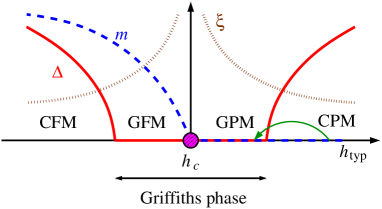
Figure S1: Schematics of the zero-temperature phase diagram of the model Hamiltonian (2) of the main text or, more generically, Eq. (S3), the corresponding spectral gap $\Delta$ (red), the order parameter $m$ (dahsed blue), and the spin-spin correlation length $\xi$ (dotted brown). The critical point at $h_{\text{typ}}=h_{c}=J_{\text{typ}}$ is surrounded by the ferromagnetic and paramagnetic Griffiths phases (GFM and GPM, respectively) where $\Delta$ vanishes. Here, CFM and CPM stand for conventional ferromagnetic and paramagnetic phases, respectively. The quantum quenches we study in this work are depicted by the (green) arrow connecting the CPM to the GPM phases.

The extent of the Griffiths phase is proportional to the disorder strength of the coupling constants. For concreteness, let $\{J_{i}\}$ be independent random variables distributed between $J_{\text{min}}<J_{i}<J_{\text{max}}$. The Griffiths paramagnetic phase covers the interval $h_{c}<h_{\text{typ}}<J_{\text{max}}$ and the Griffiths ferromagnetic phase covers the interval $J_{\text{min}}<h_{\text{typ}}<h_{c}$.

Deep in the conventional phases, the ground state is very similar to the clean one, and the system properties (like the spectral gap) are well approximated by that of the clean system with the value of the clean $J$ and $h$ being replaced by its typical values.

In this work, we show the relevance of the rare regions on the unitary dynamics after a quantum quench from the conventional paramagnetic phase to the nearby Griffiths paramagnetic phase (see green arrow in Fig. S1). In this quench, the bulk experiences a “mild” quench and, thus, remains nearly in its ground state. On the other hand, this quantum quench brings the rare regions from one phase to the other, and, thus, are highly excited.

II Mapping to free fermions, diagonalization, and observables

II.1 The mapping

Following Refs. Lieb et al., 1961; Young and Rieger, 1996, the random transverse-field Ising chain Hamiltonian with periodic boundary conditions is

$$H=-\sum_{i=1}^{L}J_{i}\sigma_{i}^{z}\sigma_{i+1}^{z}-\sum_{i=1}^{L}h_{i}\sigma_{i}^{x},$$ (S1)

which generalizes the Hamiltonian (2) of the main text, can be mapped to a free femionic one via the Jordan-Wigner transformation

$$\sigma_{j}^{x}=1-2n_{j}=c_{j}^{\phantom{\dagger}}c_{j}^{\dagger}-c_{j}^{\dagger}c_{j}^{\phantom{\dagger}},\quad\sigma_{j}^{y}=ie^{i\pi\sum_{k=1}^{j-1}n_{k}}\left(c_{j}^{\dagger}-c_{j}^{\phantom{\dagger}}\right),\quad\sigma_{j}^{z}=e^{i\pi\sum_{k=1}^{j-1}n_{k}}\left(c_{j}^{\dagger}+c_{j}^{\phantom{\dagger}}\right),$$ (S2)

with $\left\{c_{i}\right\}$ being fermionic operators of spinless fermions, i.e., $\left\{c_{i}^{\dagger},c_{j}^{\dagger}\right\}=\left\{c_{i}^{\phantom{\dagger}},c_{j}^{\phantom{\dagger}}\right\}=0$ and $\left\{c_{i}^{\phantom{\dagger}},c_{j}^{\dagger}\right\}=\delta_{i,j}$. The corresponding fermionic Hamiltonian is

$$H=\left(\mathbf{c}^{\dagger}\right)^{T}\mathbb{A}\mathbf{c}-\left(\mathbf{c}\right)^{T}\mathbb{A}\mathbf{c}^{\dagger}+\left(\mathbf{c}^{\dagger}\right)^{T}\mathbb{B}\mathbf{c}^{\dagger}-\left(\mathbf{c}\right)^{T}\mathbb{B}\mathbf{c},$$ (S3)

where $\mathbf{c}^{T}=\left(c_{1}^{\phantom{\dagger}},c_{L}^{\phantom{\dagger}},\dots,c_{L}^{\phantom{\dagger}}\right)$ is a row vector operator and the matrices $\mathbb{A}$ and $\mathbb{B}$ are

$$\mathbb{A}=\frac{1}{2}\left(\begin{array}[]{ccccc}2h_{1}&-J_{1}&0&\cdots&\left(-1\right)^{N}J_{L}\\ -J_{1}&2h_{2}&-J_{2}&\cdots&0\\ 0&-J_{2}&2h_{3}&\cdots&\vdots\\ \vdots&\vdots&\vdots&\ddots&-J_{L-1}\\ \left(-1\right)^{N}J_{L}&0&\cdots&-J_{L-1}&2h_{L}\end{array}\right),\ \mathbb{B}=\frac{1}{2}\left(\begin{array}[]{ccccc}0&-J_{1}&0&\cdots&-\left(-1\right)^{N}J_{L}\\ J_{1}&0&-J_{2}&\cdots&0\\ 0&J_{2}&0&\cdots&\vdots\\ \vdots&\vdots&\vdots&\ddots&-J_{L-1}\\ \left(-1\right)^{N}J_{L}&0&\cdots&J_{L-1}&0\end{array}\right).$$ (S4)

Here, $N=\sum_{j=1}^{2L}n_{j}$ is the total number of fermions. Although $N$ it is not a conserved quantity, its parity is. Thus, $e^{i\pi N}=\left(-1\right)^{N}$ is a conserved quantity. The value of the parity is determined by that one giving the lowest ground-state energy.

II.2 Diagonalization

The diagonalization is via the Bogoliubov-Valatin transformation (Young and Rieger, 1996). Thus, defining the matrix $\mathbb{M}$ such that

$$H=\left(\begin{array}[]{cc}\mathbf{c}^{\dagger T}&\mathbf{c}^{T}\end{array}\right)\mathbb{M}\left(\begin{array}[]{c}\mathbf{c}\\ \mathbf{c}^{\dagger}\end{array}\right),\mbox{ then }\mathbb{M}=\left(\begin{array}[]{cc}\mathbb{A}&\mathbb{B}\\ -\mathbb{B}&-\mathbb{A}\end{array}\right),$$ (S5)

is a $2L\times 2L$ symmetric matrix. The matrix $\mathbb{M}$ is brought to a diagonal form $\mathbb{D}=\mathbb{V^{T}MV}$, with $\mathbb{V}$ being a matrix whose the $k$th column is the $k$th eigenvectors of $\mathbb{M}$ and $\mathbb{D}=\text{diag}\left\{\lambda_{k}\right\}$ is a diagonal matrix whose elements are the corresponding eigenenergies. It is possible to show that the eigenenergies appears in positive-negative pairs, i.e., if $\lambda>0$ is an eigenenergy of $\mathbb{M}$, so is $-\lambda$. In addition, it is possible to show that $\mathbb{V}$ can be written as

$$\mathbb{V}=\left(\begin{array}[]{cc}\mathbb{R}&\mathbb{L}\\ \mathbb{L}&\mathbb{R}\end{array}\right),$$ (S6)

where $\mathbb{R}^{T}\mathbb{R}+\mathbb{L}^{T}\mathbb{L}=\mathbb{R}\mathbb{R}^{T}+\mathbb{L}\mathbb{L}^{T}=\mathds{1}$ and $\mathbb{R}^{T}\mathbb{L}+\mathbb{L}^{T}\mathbb{R}=\mathbb{L}\mathbb{R}^{T}+\mathbb{R}\mathbb{L}^{T}=\mathbf{0}$. In addition, the first $L$ eigenenergies are $\lambda_{k}\geq 0$ while the remaining ones are negative with $\lambda_{k+L}=-\lambda_{k}$.

With these properties, the Hamiltonian can be brought to a diagonal form

$$H=\sum_{k=1}^{L}\lambda_{k}\left(\gamma_{k}^{\dagger}\gamma_{k}^{\phantom{\dagger}}-\gamma_{k}^{\phantom{\dagger}}\gamma_{k}^{\dagger}\right),$$ (S7)

where all eigenenergies $\left\{\lambda_{k}\right\}$, $k=1,\dots,L$ are non-negative, and $\left\{\gamma_{k}\right\}$ are fermionic operators which are related to the original fermions via

$$\mathbf{c}=\mathbb{R}\boldsymbol{\gamma}+\mathbb{L}\boldsymbol{\gamma}^{\dagger},\mbox{ and }\boldsymbol{\gamma}=\mathbb{R}^{T}\mathbf{c}+\mathbb{L}^{T}\mathbf{c}^{\dagger}.$$ (S8)

In order to determine the parity $\left(-1\right)^{N}$ of the ground state, we need, in general, to diagonalize $\mathbb{M}$ with both parities and pick up the one yielding the lowest ground state energy

$$E_{\text{GS}}=-\sum_{k=1}^{L}\lambda_{k}.$$ (S9)

Once the parity is determined for the pre-quench Hamiltonian, it is conserved by the post-quench Hamiltonian.

II.3 The dynamical partition function

We now want to compute the return probability amplitude [Eq. (1) of the main text]

$$Z\left(z\right)=\left\langle\psi_{0}\left|e^{-iHz}\right|\psi_{0}\right\rangle\equiv\left\langle e^{-iHz}\right\rangle_{0},$$ (S10)

where $\left|\psi_{0}\right\rangle$ is the ground state of the pre-quench Hamiltonian $H_{0}$, $H$ is the post-quench Hamiltonian, and $z=t+i\tau$ is the complex time. Evidently, we are assuming that $H_{0}$ and $H$ can be written as free-fermionic Hamiltonians (S3).

Following (Lieb et al., 1961), we recast

$$e^{-iHz} = \prod_{k=1}^{L}e^{-i\lambda_{k}z\left(\gamma_{k}^{\dagger}\gamma_{k}^{\phantom{\dagger}}-\gamma_{k}^{\phantom{\dagger}}\gamma_{k}^{\dagger}\right)}=e^{-iE_{\text{GS}}z}\prod_{k=1}^{L}e^{-i2\lambda_{k}z\left(\gamma_{k}^{\dagger}\gamma_{k}^{\phantom{\dagger}}\right)}$$ (S11)

$$= e^{-iE_{\text{GS}}z}\prod_{k=1}^{L}\left(e^{-2i\lambda_{k}z}\gamma_{k}^{\dagger}+\gamma_{k}^{\phantom{\dagger}}\right)\left(\gamma_{k}^{\dagger}+\gamma_{k}^{\phantom{\dagger}}\right)=e^{-iE_{\text{GS}}z}\prod_{k=1}^{L}A_{k}B_{k},$$

where the vector operators

$$\mathbf{A} = e^{-2i\boldsymbol{\lambda}z}\boldsymbol{\gamma}^{\dagger}+\boldsymbol{\gamma}=\left(\mathbb{L}^{T}+e^{-2i\boldsymbol{\lambda}z}\mathbb{R}^{T}\right)\mathbf{c}^{\dagger}+\left(e^{-2i\boldsymbol{\lambda}z}\mathbb{L}^{T}+\mathbb{R}^{T}\right)\mathbf{c}$$ (S12)

$$= \left(\mathbb{L}^{T}+e^{-2i\boldsymbol{\lambda}z}\mathbb{R}^{T}\right)\left(\mathbb{R}_{0}\boldsymbol{\gamma}_{0}^{\dagger}+\mathbb{L}_{0}\boldsymbol{\gamma}_{0}^{\phantom{\dagger}}\right)+\left(e^{-2i\boldsymbol{\lambda}z}\mathbb{L}^{T}+\mathbb{R}^{T}\right)\left(\mathbb{R}_{0}\boldsymbol{\gamma}_{0}^{\phantom{\dagger}}+\mathbb{L}_{0}\boldsymbol{\gamma}_{0}^{\dagger}\right),$$

$$\mathbf{B} = \boldsymbol{\gamma}^{\dagger}+\boldsymbol{\gamma}=\left(\mathbb{L}^{T}+\mathbb{R}^{T}\right)\left(\mathbb{L}_{0}+\mathbb{R}_{0}\right)\left(\boldsymbol{\gamma}_{0}^{\dagger}+\boldsymbol{\gamma}_{0}^{\phantom{\dagger}}\right).$$ (S13)

Here, $e^{-2i\boldsymbol{\lambda}z}$ is a $L\times L$ diagonal matrix with the $k$th diagonal element $e^{-2i\lambda_{k}z}$, and $\boldsymbol{\gamma}^{T}=\left(\gamma_{1},\dots,\gamma_{L}\right)$ with $\left\{\lambda_{k}\right\}$ being the eigenfermions of the post-quench Hamiltonian. Likewise, $\boldsymbol{\gamma}_{0}^{T}$ is the analog for $H_{0}$.

The mean value $\left\langle e^{-iHz}\right\rangle_{0}$ is obtained by the use of the Wick’s theorem. We then need all non-vanishing contractions of $\prod_{k=1}^{L}A_{k}B_{k}$. The contractions of type $\left\langle A_{j}A_{k}\right\rangle$ do not give a diagonal matrix, but the contraction of the $B$’s does:

$$\left\langle\mathbf{B}\mathbf{B}^{T}\right\rangle=\left(\mathbb{L}^{T}+\mathbb{R}^{T}\right)\left(\mathbb{L}_{0}+\mathbb{R}_{0}\right)\left\langle\left(\boldsymbol{\gamma}_{0}^{\dagger}+\boldsymbol{\gamma}_{0}^{\phantom{\dagger}}\right)\left(\boldsymbol{\gamma}_{0}^{\dagger T}+\boldsymbol{\gamma}_{0}^{T}\right)\right\rangle_{0}\left(\mathbb{L}_{0}^{T}+\mathbb{R}_{0}^{T}\right)\left(\mathbb{L}+\mathbb{R}\right)=\mathds{1},$$

since $\left\langle\boldsymbol{\gamma}_{0}^{\dagger}\boldsymbol{\gamma}_{0}^{\dagger T}\right\rangle_{0}=\left\langle\boldsymbol{\gamma}_{0}^{\dagger}\boldsymbol{\gamma}_{0}^{T}\right\rangle_{0}=\left\langle\boldsymbol{\gamma}_{0}^{\phantom{\dagger}}\boldsymbol{\gamma}_{0}^{T}\right\rangle_{0}=\mathbf{0}$ and $\left\langle\boldsymbol{\gamma}_{0}^{\phantom{\dagger}}\boldsymbol{\gamma}_{0}^{\dagger T}\right\rangle_{0}=\mathds{1}$, as there is no eigenfermion in the ground state of $H_{0}$. Therefore, all contractions must be of type $\left\langle A_{i}B_{j}\right\rangle$. A contraction of type $\left\langle A_{i}A_{j}\right\rangle$ is not necessarily vanishing, however, it must be multiplied by a contraction of type $\left\langle B_{m}B_{n}\right\rangle$ which vanishes since $m\neq n$. Finally, we have that

$$\left\langle e^{-iHz}\right\rangle_{0}=e^{-iE_{\text{GS}}z}\left\langle\prod_{k=1}^{L}A_{k}B_{k}\right\rangle_{0}=e^{-iE_{\text{GS}}z}\det\left(\begin{array}[]{cccc}\left\langle A_{1}B_{1}\right\rangle_{0}&\left\langle A_{1}B_{2}\right\rangle_{0}&\cdots&\left\langle A_{1}B_{L}\right\rangle_{0}\\ \left\langle A_{2}B_{1}\right\rangle_{0}&\left\langle A_{2}B_{2}\right\rangle_{0}&\cdots&\left\langle A_{2}B_{L}\right\rangle_{0}\\ \vdots&\vdots&\ddots&\vdots\\ \left\langle A_{L}B_{1}\right\rangle_{0}&\left\langle A_{L}B_{2}\right\rangle_{0}&\cdots&\left\langle A_{L}B_{L}\right\rangle_{0}\end{array}\right)=e^{-iE_{\text{GS}}z}\det\left\langle\mathbf{A}\mathbf{B}^{T}\right\rangle_{0}.$$ (S14)

The mean value

$$\left\langle\mathbf{A}\mathbf{B}^{T}\right\rangle_{0} = \left[\left(\mathbb{L}^{T}+e^{-2i\boldsymbol{\lambda}z}\mathbb{R}^{T}\right)\mathbb{L}_{0}+\left(e^{-2i\boldsymbol{\lambda}z}\mathbb{L}^{T}+\mathbb{R}^{T}\right)\mathbb{R}_{0}\right]\left\langle\boldsymbol{\gamma}_{0}^{\phantom{\dagger}}\boldsymbol{\gamma}_{0}^{\dagger}\right\rangle_{0}\left(\mathbb{L}_{0}^{T}+\mathbb{R}_{0}^{T}\right)\left(\mathbb{L}+\mathbb{R}\right)$$

$$= \left[e^{-2i\boldsymbol{\lambda}z}\left(\mathbb{R}^{T}\mathbb{L}_{0}+\mathbb{L}^{T}\mathbb{R}_{0}\right)+\mathbb{L}^{T}\mathbb{L}_{0}+\mathbb{R}^{T}\mathbb{R}_{0}\right]\left(\mathbb{L}_{0}^{T}+\mathbb{R}_{0}^{T}\right)\left(\mathbb{L}+\mathbb{R}\right).$$

Summarizing,

$$Z\left(z\right)=e^{-iE_{\text{GS}}z}\det\left[\left(e^{-2i\boldsymbol{\lambda}z}-\mathds{1}\right)\left(\mathbb{R}^{T}\mathbb{L}_{0}+\mathbb{L}^{T}\mathbb{R}_{0}\right)\left(\mathbb{L}_{0}^{T}+\mathbb{R}_{0}^{T}\right)\left(\mathbb{L}+\mathbb{R}\right)+\mathds{1}\right].$$ (S15)

We checked this result against exact diagonalization of (S1) in the spin basis for various quantum quenches, complex time instants $z$, coupling configurations $\left\{J_{i}\right\}$, and chain sizes from $L=4$ to $8$. The difference is within machine precision.

II.4 Energy density and current

The energy current operator is obtained in the following manner. Define the energy density operator as

$$E_{i}=-\frac{1}{2}J_{i-1}\sigma_{i-1}^{z}\sigma_{i}^{z}-h_{i}\sigma_{i}^{x}-\frac{1}{2}J_{i}\sigma_{i}^{z}\sigma_{i+1}^{z}.$$ (S16)

The Hamiltonian is $H=\sum_{i}E_{i}$ and is a conserved quantity. Thus, there is a continuity equation

$$\frac{\partial{\cal E}_{i}}{\partial t}+\nabla\cdot{\cal J}=\frac{\partial{\cal E}_{i}}{\partial t}+\left({\cal J}_{i+1}-{\cal J}_{i}\right)=0,$$

where ${\cal E}_{i}=\left\langle\psi\left(t\right)\left|E_{i}\right|\psi\left(t\right)\right\rangle$, ${\cal J}_{i}=\left\langle\psi\left(t\right)\left|I_{i}\right|\psi\left(t\right)\right\rangle$ is the mean value of the associated local energy current operator, and we have taken the discrete divergent considering the lattice spacing as 1. The energy current operator is obtained from the continuity equation

$$\frac{\partial{\cal E}_{i}}{\partial t}=i\left\langle\left[H,E_{i}\right]\right\rangle.$$

The commutator is simply

$$\left[H,E_{i}\right] = i\left[J_{i}\left(-h_{i+1}\sigma_{i}^{z}\sigma_{i+1}^{y}+h_{i}\sigma_{i}^{y}\sigma_{i+1}^{z}\right)-J_{i-1}\left(-h_{i}\sigma_{i-1}^{z}\sigma_{i}^{y}+h_{i-1}\sigma_{i-1}^{y}\sigma_{i}^{z}\right)\right]=i\left(I_{i+1}-I_{i}\right),$$

i.e., the current operator is

$$I_{j}=J_{j-1}\left(-h_{j}\sigma_{j-1}^{z}\sigma_{j}^{y}+h_{j-1}\sigma_{j-1}^{y}\sigma_{j}^{z}\right).$$ (S17)

This recovers the current operator quoted in the main text. In the free-fermionic language (S2),

$$E_{j} = -\frac{1}{2}J_{j-1}\left(c_{j-1}^{\dagger}-c_{j-1}^{\phantom{\dagger}}\right)\left(c_{j}^{\dagger}+c_{j}^{\phantom{\dagger}}\right)+h_{j}\left(c_{j}^{\dagger}-c_{j}^{\phantom{\dagger}}\right)\left(c_{j}^{\dagger}+c_{j}^{\phantom{\dagger}}\right)-\frac{1}{2}J_{j}\left(c_{j}^{\dagger}-c_{j}^{\phantom{\dagger}}\right)\left(c_{j+1}^{\dagger}+c_{j+1}^{\phantom{\dagger}}\right),$$ (S18)

$$I_{j} = iJ_{j-1}\left[-h_{j}\left(c_{j-1}^{\dagger}-c_{j-1}^{\phantom{\dagger}}\right)\left(c_{j}^{\dagger}-c_{j}^{\phantom{\dagger}}\right)+h_{j-1}\left(c_{j-1}^{\dagger}+c_{j-1}^{\phantom{\dagger}}\right)\left(c_{j}^{\dagger}+c_{j}^{\phantom{\dagger}}\right)\right].$$ (S19)

For the boundary terms, one simply replaces $j-1=0\rightarrow L$, $j+1=L+1\rightarrow 1$, and multiplies the resulting term by $\left(-1\right)^{N+1}$.

The average values of $\left(c_{j-1}^{\dagger}-c_{j-1}^{\phantom{\dagger}}\right)\left(c_{j}^{\dagger}+c_{j}^{\phantom{\dagger}}\right)$, $\left(c_{j-1}^{\dagger}-c_{j-1}^{\phantom{\dagger}}\right)\left(c_{j}^{\dagger}-c_{j}^{\phantom{\dagger}}\right)$ and $\left(c_{j-1}^{\dagger}+c_{j-1}^{\phantom{\dagger}}\right)\left(c_{j}^{\dagger}+c_{j}^{\phantom{\dagger}}\right)$ (and the corresponding boundary terms) are needed. They all can be obtained in the following unified way. Let $x=\pm 1$ and $y=\pm 1$, then

$$\left\langle\left(\mathbf{c}^{\dagger}+x\mathbf{c}\right)\left(\mathbf{c}^{\dagger T}+y\mathbf{c}^{T}\right)\right\rangle = \mathbb{P}_{x}\left(ye^{2i\boldsymbol{\lambda}t}\left\langle\boldsymbol{\gamma}^{\dagger}\boldsymbol{\gamma}^{T}\right\rangle_{0}e^{-2i\boldsymbol{\lambda}t}+e^{2i\boldsymbol{\lambda}t}\left\langle\boldsymbol{\gamma}^{\dagger}\boldsymbol{\gamma}^{\dagger T}\right\rangle_{0}e^{2i\boldsymbol{\lambda}t}\right.$$ (S20)

$$\left.+xye^{-2i\boldsymbol{\lambda}t}\left\langle\boldsymbol{\gamma}\boldsymbol{\gamma}^{T}\right\rangle_{0}e^{-2i\boldsymbol{\lambda}t}+xe^{-2i\boldsymbol{\lambda}t}\left\langle\boldsymbol{\gamma}\boldsymbol{\gamma}^{\dagger T}\right\rangle_{0}e^{2i\boldsymbol{\lambda}t}\right)\mathbb{P}_{y}^{T},$$

where $\mathbb{P}_{x}=\mathbb{R}+x\mathbb{L}$ and we have used Eq. (S8). It is a tedious algebra to show that

$$\left\langle\boldsymbol{\gamma}^{\dagger}\boldsymbol{\gamma}^{\dagger T}\right\rangle_{0} = \mathbb{R}^{T}\mathbb{L}_{0}\mathbb{R}_{0}^{T}\mathbb{R}+\mathbb{R}^{T}\mathbb{L}_{0}\mathbb{L}_{0}^{T}\mathbb{L}+\mathbb{L}^{T}\mathbb{R}_{0}\mathbb{R}_{0}^{T}\mathbb{R}+\mathbb{L}^{T}\mathbb{R}_{0}\mathbb{L}_{0}\mathbb{L},$$ (S21)

$$\left\langle\boldsymbol{\gamma}^{\dagger}\boldsymbol{\gamma}^{T}\right\rangle_{0} = \mathbb{R}^{T}\mathbb{L}_{0}\mathbb{L}_{0}^{T}\mathbb{R}+\mathbb{R}^{T}\mathbb{L}_{0}\mathbb{R}_{0}^{T}\mathbb{L}+\mathbb{L}^{T}\mathbb{R}_{0}\mathbb{L}_{0}^{T}\mathbb{R}+\mathbb{L}^{T}\mathbb{R}_{0}\mathbb{R}_{0}^{T}\mathbb{L},$$ (S22)

$$\left\langle\boldsymbol{\gamma}\boldsymbol{\gamma}^{\dagger T}\right\rangle_{0} = \mathbb{R}^{T}\mathbb{R}_{0}\mathbb{R}_{0}^{T}\mathbb{R}+\mathbb{R}^{T}\mathbb{R}_{0}\mathbb{L}_{0}^{T}\mathbb{L}+\mathbb{L}^{T}\mathbb{L}_{0}\mathbb{R}_{0}^{T}\mathbb{R}+\mathbb{L}^{T}\mathbb{L}_{0}\mathbb{L}_{0}^{T}\mathbb{L},$$ (S23)

$$\left\langle\boldsymbol{\gamma}\boldsymbol{\gamma}^{T}\right\rangle_{0} = \mathbb{R}^{T}\mathbb{R}_{0}\mathbb{L}_{0}^{T}\mathbb{R}+\mathbb{R}^{T}\mathbb{R}_{0}\mathbb{R}_{0}^{T}\mathbb{L}+\mathbb{L}^{T}\mathbb{L}_{0}\mathbb{L}_{0}^{T}\mathbb{R}+\mathbb{L}^{T}\mathbb{L}_{0}\mathbb{R}_{0}^{T}\mathbb{L}.$$ (S24)

It is curious to notice that $\left\langle\boldsymbol{\gamma}\boldsymbol{\gamma}^{T}\right\rangle_{0}^{T}=\left\langle\boldsymbol{\gamma}^{\dagger}\boldsymbol{\gamma}^{\dagger T}\right\rangle_{0},\mbox{ and that }\left\langle\boldsymbol{\gamma}\boldsymbol{\gamma}^{\dagger T}\right\rangle_{0}^{T}+\left\langle\boldsymbol{\gamma}^{\dagger}\boldsymbol{\gamma}^{T}\right\rangle_{0}=\mathds{1}.$

Plugging (S21)–(S24) into (S20), we then find that

$$\left\langle\left(c_{j-1}^{\dagger}+c_{j-1}^{\phantom{\dagger}}\right)\left(c_{j}^{\dagger}+c_{j}^{\phantom{\dagger}}\right)\right\rangle$$

$$=i\sum_{k,l=1}^{L}\mathbb{P}_{j-1,k} \left(\cos\left(2\lambda_{k}t\right)\left(\mathbb{P}^{T}\mathbb{P}_{0}\mathbb{Q}_{0}^{T}\mathbb{Q}\right)_{k,l}\sin\left(2\lambda_{l}t\right)-\sin\left(2\lambda_{k}t\right)\left(\mathbb{P}^{T}\mathbb{P}_{0}\mathbb{Q}_{0}^{T}\mathbb{Q}\right)_{l,k}\cos\left(2\lambda_{l}t\right)\right)\mathbb{P}_{l,j}^{T},$$ (S25)

$$\left\langle\left(c_{j-1}^{\dagger}-c_{j-1}^{\phantom{\dagger}}\right)\left(c_{j}^{\dagger}-c_{j}^{\phantom{\dagger}}\right)\right\rangle$$

$$=i\sum_{k,l=1}^{L}\mathbb{Q}_{j-1,k} \left(\sin\left(2\lambda_{k}t\right)\left(\mathbb{P}^{T}\mathbb{P}_{0}\mathbb{Q}_{0}^{T}\mathbb{Q}\right)_{k,l}\cos\left(2\lambda_{l}t\right)-\cos\left(2\lambda_{k}t\right)\left(\mathbb{P}^{T}\mathbb{P}_{0}\mathbb{Q}_{0}^{T}\mathbb{Q}\right)_{k,l}\sin\left(2\lambda_{l}t\right)\right)\mathbb{Q}_{l,j}^{T},$$ (S26)

$$\left\langle\left(c_{j-1}^{\dagger}-c_{j-1}^{\phantom{\dagger}}\right)\left(c_{j}^{\dagger}+c_{j}^{\phantom{\dagger}}\right)\right\rangle$$

$$=-\sum_{k,l=1}^{L}\mathbb{Q}_{j-1,k} \left(\sin\left(2\lambda_{k}t\right)\left(\mathbb{P}^{T}\mathbb{P}_{0}\mathbb{Q}_{0}^{T}\mathbb{Q}\right)_{k,l}\sin\left(2\lambda_{l}t\right)+\cos\left(2\lambda_{k}t\right)\left(\mathbb{P}^{T}\mathbb{P}_{0}\mathbb{Q}_{0}^{T}\mathbb{Q}\right)_{k,l}\cos\left(2\lambda_{l}t\right)\right)\mathbb{P}_{l,j}^{T},$$ (S27)

$$\left\langle\left(c_{j}^{\dagger}-c_{j}^{\phantom{\dagger}}\right)\left(c_{j}^{\dagger}+c_{j}^{\phantom{\dagger}}\right)\right\rangle$$

$$=-\sum_{k,l=1}^{L}\tilde{\mathbb{Q}}_{j,k} \left(\sin\left(2\lambda_{k}t\right)\left(\mathbb{P}^{T}\mathbb{P}_{0}\mathbb{Q}_{0}^{T}\mathbb{Q}\right)_{k,l}\sin\left(2\lambda_{l}t\right)+\cos\left(2\lambda_{k}t\right)\left(\mathbb{P}^{T}\mathbb{P}_{0}\mathbb{Q}_{0}^{T}\mathbb{Q}\right)_{k,l}\cos\left(2\lambda_{l}t\right)\right)\mathbb{P}_{l,j}^{T}.$$ (S28)

Finally,

$${\cal E}_{j} = \frac{1}{2}J_{j-1}\sum_{k,l}\mathbb{Q}_{j-1,k}\left(\sin\left(2\lambda_{k}t\right)\left(\mathbb{P}^{T}\mathbb{P}_{0}\mathbb{Q}_{0}^{T}\mathbb{Q}\right)_{k,l}\sin\left(2\lambda_{l}t\right)+\cos\left(2\lambda_{k}t\right)\left(\mathbb{P}^{T}\mathbb{P}_{0}\mathbb{Q}_{0}^{T}\mathbb{Q}\right)_{k,l}\cos\left(2\lambda_{l}t\right)\right)\mathbb{P}_{l,j}^{T}$$ (S29)

$$-h_{j}\sum_{k,l}\mathbb{Q}_{j,k}\left(\sin\left(2\lambda_{k}t\right)\left(\mathbb{P}^{T}\mathbb{P}_{0}\mathbb{Q}_{0}^{T}\mathbb{Q}\right)_{k,l}\sin\left(2\lambda_{l}t\right)+\cos\left(2\lambda_{k}t\right)\left(\mathbb{P}^{T}\mathbb{P}_{0}\mathbb{Q}_{0}^{T}\mathbb{Q}\right)_{k,l}\cos\left(2\lambda_{l}t\right)\right)\mathbb{P}_{l,j}^{T}$$

$$+\frac{1}{2}J_{j}\sum_{k,l}\mathbb{Q}_{j,k}\left(\sin\left(2\lambda_{k}t\right)\left(\mathbb{P}^{T}\mathbb{P}_{0}\mathbb{Q}_{0}^{T}\mathbb{Q}\right)_{k,l}\sin\left(2\lambda_{l}t\right)+\cos\left(2\lambda_{k}t\right)\left(\mathbb{P}^{T}\mathbb{P}_{0}\mathbb{Q}_{0}^{T}\mathbb{Q}\right)_{k,l}\cos\left(2\lambda_{l}t\right)\right)\mathbb{P}_{l,j+1}^{T},$$

$${\cal J}_{j} = J_{j-1}\left[h_{j}\sum_{k,l}\mathbb{Q}_{j-1,k}\left(\sin\left(2\lambda_{k}t\right)\left(\mathbb{P}^{T}\mathbb{P}_{0}\mathbb{Q}_{0}^{T}\mathbb{Q}\right)_{k,l}\cos\left(2\lambda_{l}t\right)-\cos\left(2\lambda_{k}t\right)\left(\mathbb{P}^{T}\mathbb{P}_{0}\mathbb{Q}_{0}^{T}\mathbb{Q}\right)_{k,l}\sin\left(2\lambda_{l}t\right)\right)\mathbb{Q}_{l,j}^{T}\right.$$ (S30)

$$\left.-h_{j-1}\sum_{k,l}\mathbb{P}_{j-1,k}\left(\cos\left(2\lambda_{k}t\right)\left(\mathbb{P}^{T}\mathbb{P}_{0}\mathbb{Q}_{0}^{T}\mathbb{Q}\right)_{k,l}\sin\left(2\lambda_{l}t\right)-\sin\left(2\lambda_{k}t\right)\left(\mathbb{P}^{T}\mathbb{P}_{0}\mathbb{Q}_{0}^{T}\mathbb{Q}\right)_{k,l}\cos\left(2\lambda_{l}t\right)\right)\mathbb{P}_{l,j}^{T}\right].$$

For completeness, the boundary terms are

$${\cal E}_{1} = \frac{\left(-1\right)^{N+1}}{2}J_{L}\sum_{k,l}\mathbb{Q}_{L,k}\left(\sin\left(2\lambda_{k}t\right)\left(\mathbb{P}^{T}\mathbb{P}_{0}\mathbb{Q}_{0}^{T}\mathbb{Q}\right)_{k,l}\sin\left(2\lambda_{l}t\right)+\cos\left(2\lambda_{k}t\right)\left(\mathbb{P}^{T}\mathbb{P}_{0}\mathbb{Q}_{0}^{T}\mathbb{Q}\right)_{k,l}\cos\left(2\lambda_{l}t\right)\right)\mathbb{P}_{l,1}^{T}$$ (S31)

$$-h_{1}\sum_{k,l}\mathbb{Q}_{1,k}\left(\sin\left(2\lambda_{k}t\right)\left(\mathbb{P}^{T}\mathbb{P}_{0}\mathbb{Q}_{0}^{T}\mathbb{Q}\right)_{k,l}\sin\left(2\lambda_{l}t\right)+\cos\left(2\lambda_{k}t\right)\left(\mathbb{P}^{T}\mathbb{P}_{0}\mathbb{Q}_{0}^{T}\mathbb{Q}\right)_{k,l}\cos\left(2\lambda_{l}t\right)\right)\mathbb{P}_{l,1}^{T}$$

$$+\frac{1}{2}J_{1}\sum_{k,l}\mathbb{Q}_{1,k}\left(\sin\left(2\lambda_{k}t\right)\left(\mathbb{P}^{T}\mathbb{P}_{0}\mathbb{Q}_{0}^{T}\mathbb{Q}\right)_{k,l}\sin\left(2\lambda_{l}t\right)+\cos\left(2\lambda_{k}t\right)\left(\mathbb{P}^{T}\mathbb{P}_{0}\mathbb{Q}_{0}^{T}\mathbb{Q}\right)_{k,l}\cos\left(2\lambda_{l}t\right)\right)\mathbb{P}_{l,2}^{T},$$

$${\cal E}_{L} = \frac{1}{2}J_{L-1}\sum_{k,l}\mathbb{Q}_{L-1,k}\left(\sin\left(2\lambda_{k}t\right)\left(\mathbb{P}^{T}\mathbb{P}_{0}\mathbb{Q}_{0}^{T}\mathbb{Q}\right)_{k,l}\sin\left(2\lambda_{l}t\right)+\cos\left(2\lambda_{k}t\right)\left(\mathbb{P}^{T}\mathbb{P}_{0}\mathbb{Q}_{0}^{T}\mathbb{Q}\right)_{k,l}\cos\left(2\lambda_{l}t\right)\right)\mathbb{P}_{l,L}^{T}$$ (S32)

$$-h_{L}\sum_{k,l}\mathbb{Q}_{L,k}\left(\sin\left(2\lambda_{k}t\right)\left(\mathbb{P}^{T}\mathbb{P}_{0}\mathbb{Q}_{0}^{T}\mathbb{Q}\right)_{k,l}\sin\left(2\lambda_{l}t\right)+\cos\left(2\lambda_{k}t\right)\left(\mathbb{P}^{T}\mathbb{P}_{0}\mathbb{Q}_{0}^{T}\mathbb{Q}\right)_{k,l}\cos\left(2\lambda_{l}t\right)\right)\mathbb{P}_{l,L}^{T}$$

$$+\frac{\left(-1\right)^{N+1}}{2}J_{L}\sum_{k,l}\mathbb{Q}_{L,k}\left(\sin\left(2\lambda_{k}t\right)\left(\mathbb{P}^{T}\mathbb{P}_{0}\mathbb{Q}_{0}^{T}\mathbb{Q}\right)_{k,l}\sin\left(2\lambda_{l}t\right)+\cos\left(2\lambda_{k}t\right)\left(\mathbb{P}^{T}\mathbb{P}_{0}\mathbb{Q}_{0}^{T}\mathbb{Q}\right)_{k,l}\cos\left(2\lambda_{l}t\right)\right)\mathbb{P}_{l,1}^{T},$$

$${\cal J}_{1} = \left(-1\right)^{N+1}J_{L}\left[h_{1}\sum_{k,l}\mathbb{Q}_{L,k}\left(\sin\left(2\lambda_{k}t\right)\left(\mathbb{P}^{T}\mathbb{P}_{0}\mathbb{Q}_{0}^{T}\mathbb{Q}\right)_{k,l}\cos\left(2\lambda_{l}t\right)-\cos\left(2\lambda_{k}t\right)\left(\mathbb{P}^{T}\mathbb{P}_{0}\mathbb{Q}_{0}^{T}\mathbb{Q}\right)_{k,l}\sin\left(2\lambda_{l}t\right)\right)\mathbb{Q}_{l,1}^{T}\right.$$ (S33)

$$\left.-h_{L}\sum_{k,l}\mathbb{P}_{L,k}\left(\cos\left(2\lambda_{k}t\right)\left(\mathbb{P}^{T}\mathbb{P}_{0}\mathbb{Q}_{0}^{T}\mathbb{Q}\right)_{k,l}\sin\left(2\lambda_{l}t\right)-\sin\left(2\lambda_{k}t\right)\left(\mathbb{P}^{T}\mathbb{P}_{0}\mathbb{Q}_{0}^{T}\mathbb{Q}\right)_{k,l}\cos\left(2\lambda_{l}t\right)\right)\mathbb{P}_{l,1}^{T}\right].$$

In the main text, we are interested in the mean energy density above the ground state of the post-quench Hamiltonian

$$\delta{\cal E}_{j}(t)={\cal E}_{j}(t)-{\cal E}_{j}^{(\text{GS})},$$ (S34)

where ${\cal E}_{j}^{(\text{GS})}=\left\langle\phi_{\text{GS}}\left|E_{j}\right|\phi_{\text{GS}}\right\rangle$ and $\left|\phi_{\text{GS}}\right\rangle$ is the ground state of the post-quench Hamiltonian $H$. This is easily computed. Coming back to (S18), we then need the analogous of (S20) which is $\left\langle\left(\mathbf{c}^{\dagger}+x\mathbf{c}\right)\left(\mathbf{c}^{\dagger T}+y\mathbf{c}^{T}\right)\right\rangle_{\text{GS}}=x\mathbb{P}_{x}\mathbb{P}_{y}^{T}.$ Then,

$${\cal E}_{j}^{(\text{GS})} = \frac{1}{2}J_{j-1}\sum_{k}\mathbb{Q}_{j-1,k}\mathbb{P}_{j,k}-h_{j}\sum_{k}\mathbb{Q}_{j,k}\mathbb{P}_{j,k}+\frac{1}{2}J_{j}\sum_{k}\mathbb{Q}_{j,k}\mathbb{P}_{j+1,k}$$ (S35)

$$= \frac{1}{2}J_{j-1}\left(\mathbb{Q}\mathbb{P}^{T}\right)_{j-1,j}-h_{j}\left(\mathbb{Q}\mathbb{P}^{T}\right)_{j,j}+\frac{1}{2}J_{j}\left(\mathbb{Q}\mathbb{P}^{T}\right)_{j,j+1},$$

$${\cal E}_{1}^{(\text{GS})} = \frac{\left(-1\right)^{N+1}}{2}J_{L}\left(\mathbb{Q}\mathbb{P}^{T}\right)_{L,1}-h_{1}\left(\mathbb{Q}\mathbb{P}^{T}\right)_{1,1}+\frac{1}{2}J_{1}\left(\mathbb{Q}\mathbb{P}^{T}\right)_{1,2},$$ (S36)

$${\cal E}_{L}^{(\text{GS})} = \frac{1}{2}J_{L-1}\left(\mathbb{Q}\mathbb{P}^{T}\right)_{L-1,L}-h_{L}\left(\mathbb{Q}\mathbb{P}^{T}\right)_{L,L}+\frac{\left(-1\right)^{N+1}}{2}J_{L}\left(\mathbb{Q}\mathbb{P}^{T}\right)_{L,1}.$$ (S37)

III The clean transverse-field Ising chain

III.1 Diagonalization

The model Hamiltonian is

$$H=-J\sum_{i=1}^{L}\sigma_{j}^{z}\sigma_{j+1}^{z}-h\sum_{j=1}^{L}\sigma_{j}^{x},$$ (S38)

where we are using periodic boundary conditions $\sigma_{L}^{x}\sigma_{L+1}^{x}=\sigma_{L}^{x}\sigma_{1}^{x}$. From the mapping (S2), then

$$H=-J\sum_{j=1}^{L-1}\left(c_{j}^{\dagger}-c_{j}^{\phantom{\dagger}}\right)\left(c_{j+1}^{\dagger}+c_{j+1}^{\phantom{\dagger}}\right)+Je^{i\pi N}\left(c_{L}^{\dagger}-c_{L}^{\phantom{\dagger}}\right)\left(c_{1}^{\dagger}+c_{1}^{\phantom{\dagger}}\right)+h\sum_{j=1}^{L}\left(c_{j}^{\dagger}c_{j}^{\phantom{\dagger}}-c_{j}^{\phantom{\dagger}}c_{j}^{\dagger}\right).$$ (S39)

Thus, the fermionic problem has periodic boundary conditions if the total number of fermions is odd, and anti-periodic boundary conditions otherwise.

Now, we use the Fourier transformation

$$c_{j}=\sqrt{\frac{1}{L}}\sum_{n=1}^{L}e^{ik_{n}j}\gamma_{k_{n}}=\sqrt{\frac{1}{L}}\sum_{k}e^{ikj}\gamma_{k},\mbox{ where }k=k_{n}=\frac{\pi}{L}\left(2n-\frac{1+\left(-1\right)^{N+L}}{2}\right)-\pi,\ n=1,\dots,L.$$ (S40)

Then,

$$H = 2\sum_{0<k<\pi}\left(\begin{array}[]{cc}\gamma_{k}^{\dagger}&\gamma_{-k}^{\phantom{\dagger}}\end{array}\right)\left(\begin{array}[]{cc}h-J\cos k&-iJ\sin k\\ iJ\sin k&J\cos k-h\end{array}\right)\left(\begin{array}[]{c}\gamma_{k}^{\phantom{\dagger}}\\ \gamma_{-k}^{\dagger}\end{array}\right)$$ (S47)

$$+\left(h+J\right)\delta_{\left(N+L+1\right)\text{mod}2,0}\left(\gamma_{\pi}^{\dagger}\gamma_{\pi}^{\phantom{\dagger}}-\gamma_{\pi}^{\phantom{\dagger}}\gamma_{\pi}^{\dagger}\right)+\left(h-J\right)\delta_{\left(N+1\right)\text{mod}2,0}\left(\gamma_{0}^{\dagger}\gamma_{0}^{\phantom{\dagger}}-\gamma_{0}^{\phantom{\dagger}}\gamma_{0}^{\dagger}\right).$$

The modes $0$ and $\pi$ (when existing) are already diagonal. We then diagonalize the remaining ones. This can be done by finding the eigenvectors of the corresponding matrix (which is the Bogoliubov transformation). Then,

$$\mathbb{D}_{k}=\mathbb{V}_{k}^{*T}\left(\begin{array}[]{cc}h-J\cos k&-iJ\sin k\\ iJ\sin k&J\cos k-h\end{array}\right)\mathbb{V}_{k}=\left(\begin{array}[]{cc}\epsilon_{k}&0\\ 0&-\epsilon_{k}\end{array}\right),$$ (S48)

where $\mathbb{V}_{k}=\left(\begin{array}[]{cc}\cos\theta&i\sin\theta\\ i\sin\theta&\cos\theta\end{array}\right)$ is the eigenvector matrix and the dispersion relation is

$$\omega_{k}=\sqrt{h^{2}-2hJ\cos k+J^{2}}.$$ (S49)

The angle $\theta$ is such that

$$\mathbb{D}_{k}=\left(\begin{array}[]{cc}h\cos\left(2\theta\right)-J\cos\left(k+2\theta\right)&i\left(h\sin\left(2\theta\right)-J\sin\left(k+2\theta\right)\right)\\ -i\left(h\sin\left(2\theta\right)-J\sin\left(k+2\theta\right)\right)&J\cos\left(k+2\theta\right)-h\cos\left(2\theta\right)\end{array}\right)=\left(\begin{array}[]{cc}\omega_{k}&0\\ 0&-\omega_{k}\end{array}\right),$$ (S50)

and thus,

$$\tan\left(2\theta\right)=\frac{J\sin k}{h-J\cos k},\ \cos\left(2\theta\right)=\frac{h-J\cos k}{\omega_{k}},\ \sin\left(2\theta\right)=\frac{J\sin k}{\omega_{k}}.$$ (S51)

Thus, the eigenfermions are

$$\left(\begin{array}[]{c}\eta_{k}^{\phantom{\dagger}}\\ \eta_{-k}^{\dagger}\end{array}\right)=\mathbb{V}_{k}^{*T}\left(\begin{array}[]{c}\gamma_{k}^{\phantom{\dagger}}\\ \gamma_{-k}^{\dagger}\end{array}\right)=\left(\begin{array}[]{cc}\cos\theta&-i\sin\theta\\ -i\sin\theta&\cos\theta\end{array}\right)\left(\begin{array}[]{c}\gamma_{k}^{\phantom{\dagger}}\\ \gamma_{-k}^{\dagger}\end{array}\right)=\left(\begin{array}[]{c}\cos\theta\gamma_{k}^{\phantom{\dagger}}-i\sin\theta\gamma_{-k}^{\dagger}\\ \cos\theta\gamma_{-k}^{\dagger}-i\sin\theta\gamma_{k}^{\phantom{\dagger}}\end{array}\right).$$ (S52)

The inverse transformation is

$$\left(\begin{array}[]{c}\gamma_{k}^{\phantom{\dagger}}\\ \gamma_{-k}^{\dagger}\end{array}\right)=\mathbb{V}_{k}\left(\begin{array}[]{c}\eta_{k}^{\phantom{\dagger}}\\ \eta_{-k}^{\dagger}\end{array}\right)=\left(\begin{array}[]{c}\cos\theta\eta_{k}^{\phantom{\dagger}}+i\sin\theta\eta_{-k}^{\dagger}\\ \cos\theta\eta_{-k}^{\dagger}+i\sin\theta\eta_{k}^{\phantom{\dagger}}\end{array}\right).$$ (S53)

Finally, the Hamiltonian is

$$H = \sum_{k}2\omega_{k}\left(\eta_{k}^{\dagger}\eta_{k}^{\phantom{\dagger}}-\frac{1}{2}\right).$$ (S54)

Notice that the modes $k=0$ and $\pi$ are trivial $\eta_{0}=\gamma_{0}$ and $\eta_{\pi}=\gamma_{\pi}$ and we are assuming, for simplicity, that $h>J$. The ground-state energy is $E_{\text{GS}}=-\sum_{k}\omega_{k}$.

III.2 The return probability amplitude

We now want to compute the dynamical partition function

$$Z\left(z\right)=\left\langle\text{GS}\left|e^{-iHz}\right|\text{GS}\right\rangle,$$ (S55)

where the post-quench Hamiltonian is $H=2\sum_{0<k<\pi}\omega_{k}\left(\eta_{k}^{\dagger}\eta_{k}^{\phantom{\dagger}}-\eta_{-k}^{\phantom{\dagger}}\eta_{-k}^{\dagger}\right)+H_{k=0}+H_{k=\pi}$, with $H_{0,\pi}$ being the terms of the Hamiltonian concerning the trivial modes ($\eta_{0,\pi}=\eta_{0,\pi}^{(0)}$) and, therefore, contribute to $Z(z)$ with only a trivial dynamical phase. Notice that the Fourier moments $k$ are not changed by the quench. Thus, the problem simplifies in computing the $Z(z)$ for each $\pm k$ pair of modes:

$$Z\left(z\right) = \prod_{0<k<\pi}\left\langle\text{GS}_{-k}^{(0)},\text{GS}_{k}^{(0)}\left|e^{-i2\omega_{k}z\left(\eta_{k}^{\dagger}\eta_{k}^{\phantom{\dagger}}-\eta_{-k}^{\phantom{\dagger}}\eta_{-k}^{\dagger}\right)}\right|\text{GS}_{-k}^{(0)},\text{GS}_{k}^{(0)}\right\rangle$$ (S56)

$$= \prod_{0<k<\pi}\left\langle\left[1+\left(x^{-1}-1\right)\eta_{k}^{\dagger}\eta_{k}^{\phantom{\dagger}}\right]\left[1+\left(x-1\right)\eta_{-k}^{\phantom{\dagger}}\eta_{-k}^{\dagger}\right]\right\rangle_{0},$$

where $x=e^{2i\omega_{k}z}$. We need the relation between the new and old eigen-fermions.

$$\left(\begin{array}[]{c}\eta_{k}^{\phantom{\dagger}}\\ \eta_{-k}^{\dagger}\end{array}\right)=\mathbb{V}_{k}^{*T}\left(\begin{array}[]{c}\gamma_{k}^{\phantom{\dagger}}\\ \gamma_{-k}^{\dagger}\end{array}\right)=\mathbb{V}_{k}^{*T}\mathbb{V}_{k}^{(0)}\left(\begin{array}[]{c}\eta_{k}^{(0)}\\ \eta_{-k}^{(0)\dagger}\end{array}\right)=\left(\begin{array}[]{cc}\cos\left(\Delta\theta\right)&-i\sin\left(\Delta\theta\right)\\ -i\sin\left(\Delta\theta\right)&\cos\left(\Delta\theta\right)\end{array}\right)\left(\begin{array}[]{c}\eta_{k}^{(0)}\\ \eta_{-k}^{(0)\dagger}\end{array}\right),$$ (S57)

where $\Delta\theta=\theta-\theta^{(0)}$. The ground-state mean value of

$$1+\left(x^{-1}-1\right)\eta_{k}^{\dagger}\eta_{k}^{\phantom{\dagger}}+\left(x-1\right)\eta_{-k}^{\phantom{\dagger}}\eta_{-k}^{\dagger}+\left(x^{-1}-1\right)\left(x-1\right)\eta_{k}^{\dagger}\eta_{k}^{\phantom{\dagger}}\eta_{-k}^{\phantom{\dagger}}\eta_{-k}^{\dagger},$$ (S58)

is

$$1+\left(x^{-1}-1\right)\sin^{2}\Delta\theta+\left(x-1\right)\cos^{2}\Delta\theta=x^{-1}\sin^{2}\Delta\theta+x\cos^{2}\Delta\theta.$$ (S59)

Inserting the trivial dynamical phases from the trivial $0$ and $\pi$ modes, then

$$Z(z) = e^{-iE_{\text{GS}}z}\prod_{0<k<\pi}\left(1-\frac{1}{2}\left(1-e^{-4i\omega_{k}z}\right)\left(1-\frac{hh_{0}-\left(Jh_{0}+hJ_{0}\right)\cos k+JJ_{0}}{\omega_{k}\omega_{k}^{(0)}}\right)\right).$$ (S60)

The zeros of $Z(z)$, $z^{*}$, are given by

$$2\omega_{k}z^{*}=\left(m+\frac{1}{2}\right)\pi-\frac{i}{2}\ln\tan^{2}\Delta\theta,$$ (S61)

with $m\in\mathbb{N}$. The zeros pierce the real-time axis if $\tan^{2}\Delta\theta$ crosses the value $1$ for $0<k<\pi$. This is only possible if

$$\left(h-J\right)\left(h_{0}-J_{0}\right)<0.$$ (S62)

In other words, the zeros of $Z\left(z\right)$ crosses the real-time axis only if the quench crosses the equilibrium quantum phase transition.

Further manipulations allows us to rewrite the zeros as

$$2\omega_{k}z^{*}=\left(m+\frac{1}{2}\right)\pi+\frac{i}{2}\ln\left(\frac{\omega_{k}\omega_{k}^{(0)}+\left(hh_{0}-\left(Jh_{0}+hJ_{0}\right)\cos k+JJ_{0}\right)}{\omega_{k}\omega_{k}^{(0)}-\left(hh_{0}-\left(Jh_{0}+hJ_{0}\right)\cos k+JJ_{0}\right)}\right),$$ (S63)

which recovers Eq. (4) of the main text. How many zeros are there in a single accumulation line? From (S63), it is just the total number of $k$’s between $0$ and $\pi$ (excluding $0$ and $\pi$). From (S40), it is simply the largest integer less than $\frac{L+(1+\left(-1\right)^{N})/2}{2}$ (recall $k=\pi$ is excluded). Thus,

$$n_{\text{zeros}}=\frac{1}{2}\left(L-1+\left(-1\right)^{N}\left(1-L\text{mod}2\right)\right)=\frac{1}{2}\left(L-1+\left(-1\right)^{N}\left(\frac{1+\left(-1\right)^{L}}{2}\right)\right).$$ (S64)

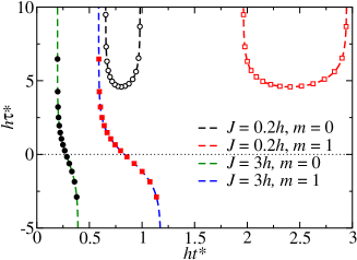
Figure S2: Zeros of the dynamical partition function for a clean chain of $30$ sites long with periodic boundary conditions (symbols) and the corresponding accumulation lines in the thermodynamic limit (dashed lines). The zeros are those given by Eq. (4) of the main text [equivalent to Eq. (S63)]. The lines are simply the zeros of the same equation with $L\rightarrow\infty$. All quantum quenches are from $h_{0}=\infty$ to finite $h$. We also show two accumulation lines $m=0$ (black and dark green) and $m=1$ (red and blue). In one chain, the coupling constants are equal to $J=0.2h$ (accumulation lines in the upper imaginary plane, black and red; open symbols), and equal to $J=3h$ in the other (accumulation lines piercing the real-time axis, dark green and blue; closed symbols).

As discussed in the main text, the zeros of $Z$ accumulate in lines which can only pierce the real-time axis if the equilibrium quantum phase transition is crossed by the quench. This is illustrated in Fig. S2. In the thermodynamic limit, the imaginary part of $z^{*}$ vanishes when $hh_{0}-\left(Jh_{0}+hJ_{0}\right)\cos k+JJ_{0}=0$. Thus, the associated momentum $q$ is given by

$$\cos q=\frac{hh_{0}+JJ_{0}}{Jh_{0}+hJ_{0}}.$$ (S65)

The corresponding zero is a real number and equals

$$t^{*}=\frac{\left(2n+1\right)\pi}{4\omega_{q}}=\frac{\left(2n+1\right)\pi}{4}\sqrt{\frac{hJ_{0}+Jh_{0}}{\left(h^{2}-J^{2}\right)\left(hJ_{0}-Jh_{0}\right)}}.$$ (S66)

For finite $L$, none of the momenta $k_{n}$ in (S40) matches $q$ in general. However, in the worst case, the closest $k_{n}$ to $q$ is far by $\delta k=\frac{2\pi}{L}$. Thus, in the large-$L$ regime, the imaginary part of the closest zero to the real-time axis vanishes as $\tau^{*}\propto\delta k\propto L^{-1}$. Although we have explicitly derived this result for a chain with periodic boundary conditions, we expect it to be valid for chains with open boundary conditions, as well. A detailed analysis will be reported elsewhere.

IV A single Rare Region

In the main text, we showed that the Yang-Lee-Fisher (YLF) zeros of the dynamical partition function $Z(z)$, Eq. (1) of the main text, perform nontrivial paths in the complex-time plane when a Rare Region (RR) appears in the system. One set of the zeros remains in the upper complex plane and the other migrates close to the real time axis. In addition, we showed that this second set of zeros $\left\{z^{*}\right\}$ and the singular part of the dynamical free-energy $f(t)$ are well described by those same quantities of a decoupled RR undergoing the same quantum quench, $\left\{z_{\text{RR}}^{*}\right\}$ and $f_{\text{RR}}$, respectively. In this section, we quantify this result. We compute the difference between $z^{*}$ and $z_{\text{RR}}^{*}$ as a function of $J_{\text{RR}}$ (the coupling constant inside the RR). This is shown in Fig. S3. As can be seen, the difference vanishes exponentially (with possible algebraic and nontrivial oscillatory corrections) with $J_{\text{RR}}$. Evidently, this behavior becomes evident when $J_{\text{RR}}$ becomes greater than $h$, as expected.

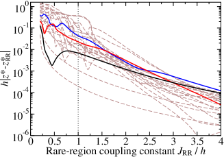
Figure S3: The absolute difference between the rare-region-induced set of zeros near the real-time axis $z^{*}$ and those of a decoupled rare region $z_{\text{RR}}^{*}$ shown in Fig. 2(b) of the main text. In total, we have compared $21$ zeros. The difference is plotted as a function of the rare-region coupling constant $J_{\text{RR}}$. The three solid lines correspond to the $3$ closest zeros to the real axis, time instants $ht\approx 0.6$ (black), $1.7$ (red), and $2.8$ (blue).

V Two Rare Regions

In the main text, we have shown that the quantum-quench-induced excitations are localized in each RR if they are sufficiently far apart from each other (see Fig. 3 of the main text). In this section, we give further evidence of this result.

In Fig. S4, we plot the dynamical free energy $f(t)$ [panel (a), continuous black line] and the corresponding zeros of $Z(z)$ [panel (b), open black circles] for a chain of $L=70$ sites long with periodic boundary conditions. The quench is from $h_{0}=\infty$ to a finite $h$. The bulk coupling constant is $J_{\text{B}}=0.2h$. The chains has two RRs. The first one is $L_{\text{RR}1}=8$ sites long and its coupling is $J_{\text{RR}1}=3h$, and the second one is $L_{\text{RR}2}=11$ sites long and its coupling is $J_{\text{RR}2}=2.5h$.

As for a single RR (see Fig. 2 of the main text), the zeros group themselves in two sets: one up in the positive complex plane and the other near the real-time axis. This second set of zeros is well approximated by decoupled RRs. We plot the dynamical free energy $f_{\text{RR}1}$ and the associated YLF zeros of the first decoupled RR as a purple dash-dotted line and purple $\times$ symbols in panel (a) and (b) of Fig. S4, respectively. Likewise for the second RR.

Interestingly, the zeros of the decoupled RRs reproduce accurately the set of zeros which accumulate in lines piercing the real-time axis. In addition, the superposition (simple sum) of the free energies of the decoupled RRs (appropriately reweighted by $L_{\text{RR}}/L$) accurately reproduce the singular part of the free energy $f$ [see red dashed line of S4(a)].

On the other hand, the set of zeros in the upper complex-time plane, which are, presumably, due to the bulk, is not well approximate by a decoupled bulk. The magenta stars in Fig. S4(b) are the YLF zeros of the decoupled bulk, i.e., the zeros corresponding to two open boundary chains of sizes $31$ and $20$ undergoing the same quantum quench from $h_{0}\rightarrow\infty$ to $h$ where the coupling constant of these chains is $J_{\text{B}}=0.2h$. This means that that analytic part of $f$ cannot be well described by decoupled bulk and rare regions.

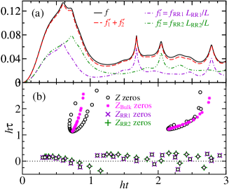
Figure S4: (a) The dynamical free energy $f$ as a function of the real time $t$ and (b) the associated Yang-Lee-Fisher zeros of the return probability amplitude $Z(z)$ with $z=t+i\tau$. The quantum quench of the Hamiltonian (2) (of the main text) is from $h_{0}=\infty$ to $h$. The chain is $70$ sites long with periodic boundary conditions. The bulk coupling constant is $J_{\text{B}}=0.2h$. The chain has two rare regions. The first (second) one comprises sites $1$ to $8$ (40 to 50). Thus, $L_{\text{RR1}}=8$ ($L_{\text{RR2}}=11$). The corresponding coupling constant is $J_{\text{RR}1}=3h$ ($J_{\text{RR}2}=2.5h$). The free energy and the corresponding zeros of the decoupled rare regions are plotted as well (see text).

VI The case of extreme quenches

Consider the simple quantum quench from

$$H_{0}=-h_{0}\sum_{i=1}^{L}\sigma_{i}^{x}\mbox{ to }H=-\sum_{i=1}^{L}J_{i}\sigma_{i}^{z}\sigma_{i+1}^{z}.$$ (S67)

The initial state is $\left|\psi_{0}\right\rangle=2^{-\frac{L}{2}}\left|\left\{s_{i}\right\}\right\rangle$, with $s_{i}=\pm 1$ and the set $\left\{s_{i}\right\}$ covers all the $2^{L}$ possible spin configurations. Thus,

$$Z=2^{-L}\sum_{\left\{s_{i}\right\}}\sum_{\left\{t_{i}\right\}}\left\langle\left\{t_{i}\right\}\left|e^{-iHz}\right|\left\{s_{i}\right\}\right\rangle=2^{-L}\sum_{\left\{s_{i}\right\}}e^{-i\left(-\sum_{k}J_{k}s_{k}s_{k+1}\right)z},$$ (S68)

which is the partition function of the classical Ising chain in zero longitudinal field. This can be computed via transfer matrix:

$$Z = 2^{-L}\text{Tr}\left[\left(\begin{array}[]{cc}e^{iJ_{1}z}&e^{-iJ_{1}z}\\ e^{-iJ_{1}z}&e^{iJ_{1}z}\end{array}\right)\left(\begin{array}[]{cc}e^{iJ_{2}z}&e^{-iJ_{2}z}\\ e^{-iJ_{2}z}&e^{iJ_{2}z}\end{array}\right)\dots\left(\begin{array}[]{cc}e^{iJ_{L}z}&e^{-iJ_{L}z}\\ e^{-iJ_{L}z}&e^{iJ_{L}z}\end{array}\right)\right]$$ (S75)

$$= \prod_{k=1}^{L}\cos\left(J_{k}z\right)+i^{L}\prod_{k=1}^{L}\sin\left(J_{k}z\right).$$ (S76)

When at least one coupling is vanishing (as for open boundary condition or as for the percolation problem), the imaginary part vanishes identically and (S76) recovers Eq. (6) of the main text.

References

Fisher (1965)M. E. Fisher, “The Nature of
Critical Points,” in Lectures in Theoretical Physics, Vol. VII C, edited by W. E. Brittin (University of Colorado
Press, Boulder, 1965).
Yang and Lee (1952)C. N. Yang and T. D. Lee, “Statistical theory of
equations of state and phase transitions. I. Theory of condensation,” Phys. Rev. 87, 404 (1952).
Peng et al. (2015)X. Peng, H. Zhou,
B.-B. Wei, J. Cui, J. Du, and R.-B. Liu, “Experimental observation of Lee-Yang zeros,” Phys. Rev. Lett. 114, 010601 (2015).
Brandner et al. (2017)K. Brandner, V. F. Maisi, J. P. Pekola, J. P. Garrahan, and C. Flindt, “Experimental determination of dynamical Lee-Yang zeros,” Phys. Rev. Lett. 118, 180601 (2017).
Imry and Ma (1975)Y. Imry and S.-k. Ma, “Random-field
instability of the ordered state of continuous symmetry,” Phys. Rev. Lett. 35, 1399 (1975).
Griffiths (1969)R. B. Griffiths, “Nonanalytic behavior above the critical point in a random Ising
ferromagnet,” Phys. Rev. Lett. 23, 17 (1969).
McCoy (1969)B. M. McCoy, “Incompleteness of the critical exponent description for ferromagnetic
systems containing random impurities,” Phys.
Rev. Lett. 23, 383
(1969).
Wortis (1974)M. Wortis, “Griffiths
singularities in the randomly dilute one-dimensional Ising model,” Phys. Rev. B 10, 4665 (1974).
Harris (1975)A. B. Harris, “Nature of the “Griffiths” singularity in dilute magnets,” Phys. Rev. B 12, 203 (1975).
Iglói and Monthus (2005)F. Iglói and C. Monthus, “Strong disorder
RG approach of random systems,” Phys. Rep. 412, 277 (2005).
Thill and Huse (1995)M. J. Thill and D. A. Huse, “Equilibrium
behaviour of quantum Ising spin glass,” Physica A 214, 321
(1995).
Vojta and Hoyos (2014)T. Vojta and J. A. Hoyos, “Criticality and
quenched disorder: Harris criterion versus rare regions,” Phys. Rev. Lett. 112, 075702 (2014).
Bloch et al. (2008)I. Bloch, J. Dalibard, and W. Zwerger, “Many-body
physics with ultracold gases,” Rev. Mod. Phys. 80, 885 (2008).
Calabrese and Cardy (2006)P. Calabrese and J. Cardy, “Time dependence
of correlation functions following a quantum quench,” Phys. Rev. Lett. 96, 136801 (2006).
Polkovnikov et al. (2011)A. Polkovnikov, K. Sengupta, A. Silva, and M. Vengalattore, “Colloquium: Nonequilibrium
dynamics of closed interacting quantum systems,” Rev.
Mod. Phys. 83, 863
(2011).
Heyl et al. (2013)M. Heyl, A. Polkovnikov, and S. Kehrein, “Dynamical quantum phase
transitions in the transverse-field Ising model,” Phys. Rev. Lett. 110, 135704 (2013).
Andraschko and Sirker (2014)F. Andraschko and J. Sirker, “Dynamical
quantum phase transitions and the loschmidt echo: A transfer matrix
approach,” Phys. Rev. B 89, 125120 (2014).
Vajna and Dóra (2014)S. Vajna and B. Dóra, “Disentangling dynamical
phase transitions from equilibrium phase transitions,” Phys.
Rev. B 89, 161105(R)
(2014).
Schmitt and Kehrein (2015)M. Schmitt and S. Kehrein, “Dynamical
quantum phase transitions in the Kitaev honeycomb model,” Phys.
Rev. B 92, 075114
(2015).
Halimeh and Zauner-Stauber (2017)J. C. Halimeh and V. Zauner-Stauber, “Dynamical phase diagram of quantum spin chains with long-range
interactions,” Phys. Rev. B 96, 134427 (2017).
Žunkovič et al. (2018)B. Žunkovič, M. Heyl,
M. Knap, and A. Silva, “Dynamical quantum phase transitions in spin
chains with long-range interactions: Merging different concepts of
nonequilibrium criticality,” Phys. Rev. Lett. 120, 130601 (2018).
Jafari (2019)R. Jafari, “Dynamical
quantum phase transition and quasi particle excitation,” Sci.
Rep. 9, 2871 (2019).
Jurcevic et al. (2017)P. Jurcevic, H. Shen,
P. Hauke, C. Maier, T. Brydges, C. Hempel, B. P. Lanyon, M. Heyl, R. Blatt, and C. F. Roos, “Direct observation of dynamical quantum
phase transitions in an interacting many-body system,” Phys. Rev. Lett. 119, 080501 (2017).
Zhang et al. (2017)J. Zhang, G. Pagano,
P. W. Hess, A. Kyprianidis, P. Becker, H. Kaplan, A. V. Gorshkov, Z.-X. Gong, and C. Monroe, “Observation of a many-body dynamical phase transition with a 53-qubit
quantum simulator,” Nature 551, 601 (2017).
Bernie et al. (2017)H. Bernie, S. Schwartz,
A. Keesling, H. Levine, A. Omran, H. Pichler, S. Choi, A. S. Zibrov, M. Endres, M. Greiner,
V. Vuletić, and M. D. Lukin, “Probing many-body dynamics on a 51-atom
quantum simulator,” Nature 551, 579 (2017).
Fläschner et al. (2018)N. Fläschner, D. Vogel,
M. Tarnowski, B. S. Rem, D.-S. Lühmann, M. Heyl, J. C. Budich, L. Mathey, K. Sengstock, and C. Weitenberg, “Observation of dynamical vortices after quenches in a system with
topology,” Nature Physics 14, 265 (2018).
Guo et al. (2019)X.-Y. Guo, C. Yang,
Y. Zeng, Y. Peng, H.-K. Li, H. Deng, Y.-R. Jin, S. Chen, D. Zheng,
and H. Fan, “Observation of a dynamical
quantum phase transition by a superconducting qubit simulation,” Phys. Rev. Applied 11, 044080 (2019).
Obuchi and Takahashi (2012)T. Obuchi and K. Takahashi, “Dynamical singularities of glassy systems in a quantum quench,” Phys. Rev. E 86, 051125 (2012).
Yang et al. (2017)C. Yang, Y. Wang,
P. Wang, X. Gao, and S. Chen, “Dynamical signature of
localization-delocalization transition in a one-dimensional incommensurate
lattice,” Phys. Rev. B 95, 184201 (2017).
Yin et al. (2018)H. Yin, S. Chen,
X. Gao, and P. Wang, “Zeros of Loschmidt echo in the presence
of Anderson localization,” Phys. Rev. A 97, 033624 (2018).
Cao et al. (2020)K. Cao, W. Li,
M. Zhong, and P. Tong, “Influence of weak disorder on the
dynamical quantum phase transitions in the anisotropic XY chain,” Phys. Rev. B 102, 014207 (2020).
Pfeuty (1979)P. Pfeuty, “An exact result
for the 1D random Ising model in a transverse field,” Phys. Lett. A 72, 245 (1979).
(46)See the Supplemental
Material, which includes Refs. Fisher, 1995; Lieb et al., 1961; Young and Rieger, 1996, for technical details and a description of our numerical approach.
Gardas et al. (2018)B. Gardas, J. Dziarmaga,
W. H. Zurek, and M. Zwolak, “Defects in quantum computers,” Sci. Rep. 8, 4539 (2018).
Fisher (1995)D. S. Fisher, “Critical behavior of random transverse-field Ising spin chains,” Phys. Rev. B 51, 6411 (1995).
Lieb et al. (1961)E. Lieb, T. Schultz, and D. Mattis, “Two soluble models of an
antiferromagnetic chain,” Ann. Phys. 16, 407 (1961).
Young and Rieger (1996)A. P. Young and H. Rieger, “Numerical study of the
random transverse-field Ising spin chain,” Phys.
Rev. B 53, 8486
(1996).
Supplementary Material for “Disorder-induced dynamical
Griffiths singularities after certain quantum quenches”