Appendix to STOPS: Short-term Volatility-controlled Policy Search and its Global Convergence

1 Notation Systems

• $(\mathcal{S},\mathcal{A},\mathcal{P},r,\gamma)$ with state space $\mathcal{S}$, action space $\mathcal{A}$, the transition kernel $\mathcal{P}$, the reward function $r$, the initial state $S_{0}$ and its distribution $\mu_{0}$, and the discounted factor $\gamma$.

• $r_{\max}>0$ is a constant as the upper bound of the reward.

• State value function $V_{\pi}(s)$ and state-action value function $Q_{\pi}(s,a)$.

• The normalized state and state action occupancy measure of policy $\pi$ is denoted by $\nu_{\pi}(s)$ and $\sigma_{\pi}(s,a)$

• $T$ is the length of a trajectory.

• The return is defined as $G$. $J(\pi)$ is the expectation of $G$.

• Policy $\pi_{\theta}$ is parameterized by the parameter $\theta$.

• $\tau$ is the temperature parameter in the softmax parameterization of the policy.

• $F(\theta)$ is the Fisher information matrix.

• $\eta_{T}D$ is the learning rate of TD update. Similarly, $\eta_{N}PG$ is the learning rate of NPG update. $\eta_{P}PO$ is the learning rate of PPO update.

• $\beta$ is the penalty factor of KL difference in PPO update.

• $f\big{(}(s,a);\theta\big{)}$ is the two-layer over-parameterized neural network, with $m$ as its width.

• $\phi_{\theta}$ is the feature mapping of the neural network.

• $\mathcal{D}$ is the parameter space for $\theta$, with $\Upsilon$ as its radius.

• $M>0$ is a constant as the initialization upper bound on $\theta$.

• $J^{G}_{\lambda}(\pi)$ is the mean-variance objective function.

• $J_{\lambda}(\pi)$ is the reward-volatility objective function, with $\lambda$ as the penalty factor.

• $J_{\lambda}^{y}(\pi)$ is the transformed reward-volatility objective function, with $y$ as the auxiliary variable.

• $\tilde{r}$ is the reward for the augmented MDP. Similarly, $\tilde{V}_{\pi}(s)$ and $\tilde{Q}_{\pi}(s,a)$ are state value function and state-action value function of the augmented MDP, respectively. $\tilde{J}(\pi)$ is the risk-neural objective of the augmented MDP.

• $\hat{y}_{k}$ is an estimator of $y$ at $k$-th iteration.

• $\omega$ is the parameter of critic network.

• $\delta_{k}=\text{argmin}_{\delta\in\mathcal{D}}\|\hat{F}(\theta_{k})\delta-\tau_{k}\hat{\nabla}_{\theta}J(\pi_{\theta_{k}})\|_{2}$.

• $\xi_{k}(\delta)=\hat{F}(\theta_{k})\delta-\tau_{k}\hat{\nabla}_{\theta}\tilde{J}(\pi_{\theta_{k}})-\mathbb{E}[\hat{F}(\theta_{k})\delta-\tau_{k}\hat{\nabla}_{\theta}\tilde{J}(\pi_{\theta_{k}})]$.

• $\sigma_{\xi}$ is a constant associated with the upper bound of the gradient variance.

• $\varphi_{k},\psi_{k},\varphi^{\prime}_{k},\psi^{\prime}_{k}$ are the concentability coefficients, upper bounded by a constant $c_{0}>0$.

• $\varphi^{*}_{k}=\mathbb{E}_{(s,a)\sim\sigma_{\pi}}\bigg{[}\big{(}\frac{d\pi^{*}}{d\pi_{0}}-\frac{d\pi_{\theta_{k}}}{d\pi_{0}}\big{)}^{2}\bigg{]}^{1/2}$.

• $\psi^{*}_{k}=\mathbb{E}_{(s,a)\sim\sigma_{\pi}}\bigg{[}\big{(}\frac{d\sigma_{\pi^{*}}}{d\sigma_{\pi}}-\frac{d\nu_{\pi^{*}}}{d\nu_{\pi}}\big{)}^{2}\bigg{]}^{1/2}$.

• $K$ is the total number of iterations. Similarly, $K_{\rm TD}$ is the total number of TD iterations.

• $c_{3}>0$ is a constant as to quantify the difference in risk-neutral objective between optimal policy and any policy.

2 Algorithm Details

We provide a comparison between MVPI and STOPS.

1 for $k=1,\dots,K$ do

2       Step 1: $y_{k}:=(1-\gamma)J(\pi_{k})$;

3       Step 2: $\tilde{J}(\pi_{\theta_{k}}):=\mathbb{E}_{(s,a)\sim\sigma_{\pi_{\theta}}}(r_{s,a}-\lambda r^{2}_{s,a}+2\lambda r_{s,a}y_{k})$;

4           if MVPI: then

5                  $\theta_{k}:=\arg\max_{\theta}(\tilde{J}(\pi_{\theta_{k}}))$;

                  // This is achieved by line 2 to 2 in Algorithm 2

6                 

7           else if STOPS: then

8                 if select NPG update then

9                        update $\theta_{k}$ according to Eq. (LABEL:eq:neural_npg_update) ;

10                       

11                 else if select PPO update then

12                        update $\theta_{k}$ according to Eq. (LABEL:eq:neural_ppo_update) ;

13                       

14                 

15           

16           

17           

18       end for

19      Output: $\pi_{\theta_{K}}$;

Algorithm 1 A comparison between STOPS and MVPI

Note that neither NPG nor PPO solve $\theta_{k}:=\arg\max_{\theta}(\tilde{J}(\pi_{\theta_{k}}))$ directly, but instead solve an approximation optimization problem at each iteration. We provide pseudo-code for the implementation of MVPI and VARAC in Algorithm 2 and 3.

1 Input: number of iteration $K$, learning rate for natural policy gradient (resp. PPO) TD $\eta_{\rm NPG}$ (resp. $\eta_{\rm PPO}$), temperature parameters $\{\tau_{k}\}^{K}_{k=1}$;

2 Initialization: Initialize policy network $f((s,a);\theta,b)$ as defined in Eq. (LABEL:eq:Theta). Set $\tau_{1}=1$. Initialize Q-network with $(b,\omega_{1})$ similarly;

3 for $k=1,\cdots,K$ do

4       Sample a batch of transitions $\{s_{t},a_{t},r_{t},s^{\prime}_{t}\}^{T}_{t=1}$ following current policy with size of $T$;

5       $y=\frac{1}{T}\sum_{t=1}^{T}r_{t}$ ;

6       for $t=1,\cdots,T$ do

7             $\tilde{r}_{t}=r_{t}-\lambda r_{t}^{2}+2\lambda r_{t}y$, $a^{\prime}_{t}\sim\pi(a|s^{\prime}_{t})$;

8            

9       end for

10      

11      repeat

12             Q-value update: update $\omega_{k}$ according to Eq. (LABEL:eq:aug_TD);

13             if select NPG update then

14                   update $\theta_{k}$ according to Eq. (LABEL:eq:neural_npg_update);

15                  

16            else if select PPO update then

17                   update $\theta_{k}$ according to Eq. (LABEL:eq:neural_ppo_update);

18                  

19      until CONVERGE;

20      

21 end for

22Output: $\pi_{\theta_{K}}$;

Algorithm 2 MVPI with over-parameterized networks

1 Input: number of iteration $K$, learning rate for natural policy gradient (resp. PPO) TD $\eta_{\rm NPG}$ (resp. $\eta_{\rm PPO}$), temperature parameters $\{\tau_{k}\}^{K}_{k=1}$;

2 Initialization: Initialize policy network $f((s,a);\theta,b)$ as defined in Eq. (LABEL:eq:Theta). Set $\tau_{1}=1$. Initialize Q-network with $(b,\omega_{1})$ similarly;

3 for $k=1,\cdots,K$ do

4       Sample a batch of transitions $\{s_{t},a_{t},r_{t},s^{\prime}_{t}\}^{T}_{t=1}$ following current policy with size of $T$;

5       $y=\frac{1}{T}\sum_{t=1}^{T}r_{t}$;

6       Q-value update: update both networks’ $\omega_{k}$ according to Eq. (LABEL:eq:aug_TD);

7       Output $Q_{k}$ and $W_{k}$;

8       update $\theta_{k}$ with NPG or PPO;

9      

10 end for

11Output: $\pi_{\theta_{K}}$;

Algorithm 3 VARAC

3 Theoretical Analysis Details

In this section, we discuss the theoretical analysis in detail. We first present the overview in Section 3.1. Then we provide additional assumptions in Section 3.2. In the rest of the section, we present all the supporting lemmas and the proof for Theorem LABEL:th:major_result_PPO and LABEL:th:major_result.

3.1 Overview

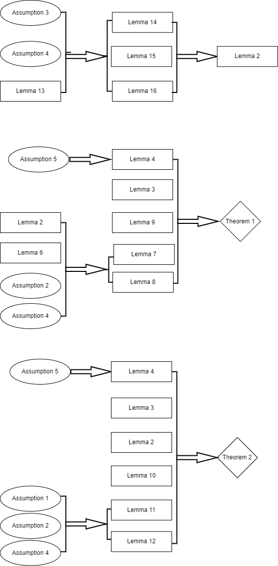
Figure 1: A flow chart of the theoretical analysis

We provide Figure 1 to illustrate the structure of the theoretical analysis. First, under Assumption 1 and 2, as well as Lemma 12. we can obtain Lemma 13, 14 and 15. These are the building blocks of lemma 1, which is a shared component in the analysis of both NPG and PPO. The shared components also include Lemma 2, as well as Lemma 3 obtained under Assumption 3. For PPO analysis, under Assumption LABEL:assu:_concentrability_regularity and 2, we obtain Lemma 6 and 7 from Lemma 1 and  5, Then combined with Lemma 2,  3 and 8, we obtain Theorem LABEL:th:major_result_PPO, the major result of PPO anaysis. Likely for NPG analysis, we first obtain Lemma 10 and 11 under Assumption LABEL:assu:_variance_regularity,  LABEL:assu:_concentrability_regularity and 2. Then together with Lemma 1, 2,  3 and 9, we obtain Theorem LABEL:th:major_result, the major result of NPG anaysis.

3.2 Additional Assumptions

Assumption 1.

(Action-value function class) We define

$$\mathcal{F}_{\Upsilon,\infty}:=\Bigg{\{}f(s,a;\theta)=f_{0}(s,a))+$$

$$\int\mathbbm{1}\{\theta^{\top}(s,a)>0\}(s,a)^{\top}\iota(\theta)d\mu(w):\|\iota(\theta)\|_{\infty}\leq\Upsilon/\sqrt{d}\Bigg{\}}$$ (1)

Where $\mu:\mathbb{R}^{d}\rightarrow[0,1]$ is a probability density function of $\mathcal{N}(0,I_{d}/d)$. $f_{0}(s,a)$ is the two-layer neural network corresponding to the initial parameter $\Theta_{{\rm init}}$, and $\iota:\mathbb{R}^{d}\rightarrow\mathbb{R}^{d}$ is a weighted function. We assume that $\tilde{Q}_{\pi}\in\mathcal{F}_{\Upsilon,\infty}$ for all $\pi$.

Assumption 2.

(Regularity of stationary distribution) For any policy $\pi$, and $\forall x\in\mathbb{R}^{d},\forall\|x\|_{2}=1$, and $\forall u>0$, we assume that there exists a constant $c>0$ such that $\mathbb{E}_{(s,a)\sim\sigma_{\pi}}\big{[}\mathbbm{1}\{|x^{\top}(s,a)|\leq u\}\big{]}\leq cu.$

Assumption 1 is a mild regularity condition on $Q_{\pi}$, as $\mathcal{F}_{\Upsilon,\infty}$ is a sufficiently rich function class and approximates a subset of the reproducing kernel Hilbert space (RKHS) [71]. Similar assumptions are widely imposed [44, 45, 46, 47, 21]. Assumption 2 is a regularity condition on the transition kernel $\mathcal{P}$. Such regularity holds so long as $\sigma_{\pi}$ has an upper bound density, satisfying most Markov chains.

In [22] Lemma 4.15, they make a mistake in the proof. They accidentally flip a sign in $y^{*}-\bar{y}$ when transitioning from the first equation in the proof to Eq.(4.15). This invalidates the conclusion in Eq.(4.17), an essential part of the proof. We tackle this issue by proposing the next assumption.

Assumption 3.

(Convergence Rate of $J(\pi)$) We assume $\pi^{*}$ (the optimal policy to the risk-averse objective function $J_{\lambda}(\pi)$) converges to the risk-neutral objective $J(\pi)$ for both NPG and PPO with the over-parameterized neural network to be $\mathcal{O}(1/\sqrt{k})$. Specifically, there exists a constant $c_{3}>0$ such that,

$$J(\pi^{*})-J(\pi_{k})\leq\frac{c_{3}}{\sqrt{k}}$$ (2)

It was proved [21, 20] that the optimal policy w.r.t the risk-neutral objective $J(\pi)$ obtained by NPG and PPO method with the over-parameterized two-layer neural network converges to the globally optimal policy at a rate of $\mathcal{O}(1/\sqrt{K})$, where $K$ is the number of iteration. Since our method uses similar settings, we assume the convergence rates of risk-neutral objective $J(\pi)$ in our paper follow their results.

In the following subsections, we study STOPS’s convergence of global optimality and provide a proof sketch.

3.3 Proof of Theorem LABEL:th:major_result_PPO

We first present the analysis of policy evaluation error, which is induced by TD update in Line LABEL:line:critic_update of Algorithm LABEL:alg:TOPS. We characterize the policy evaluation error in the following lemma:

Lemma 1.

(Policy Evaluation Error) We set learning rate of TD $\eta_{\text{TD}}=\min\{(1-\gamma)/3(1+\gamma)^{2},1/\sqrt{K_{{\rm TD}}}\}$. Under Assumption 1 and 2, it holds that, with probability of $1-\delta$,

$$\|\tilde{Q}_{\omega_{k}}-\tilde{Q}_{\pi_{k}}\|^{2}_{\nu_{\pi_{k}}}$$

$$= \mathcal{O}(\Upsilon^{3}m^{-1/2}\log(1/\delta)+\Upsilon^{5/2}m^{-1/4}\sqrt{\log(1/\delta)}$$

$$+\Upsilon r_{\max}^{2}m^{-1/4}+\Upsilon^{2}K_{{\rm TD}}^{-1/2}+\Upsilon),$$ (3)

where $\tilde{Q}_{\pi_{k}}$ is the Q-value function of the augmented MDP, and $\tilde{Q}_{\omega_{k}}$ is its estimator at the $k$-th iteration. We provide the proof and its supporting lemmas in Appendix 3.6. In the following, we establish the error induced by the policy update. Eq. (LABEL:eq:volatility_new_MDP_reward) can be re-expressed as

$$J_{\lambda}^{y}(\pi) =\sum_{s,a}\sigma_{\pi}\big{(}r_{s,a}-\lambda r_{s,a}^{2}+2\lambda r_{s,a}{y_{k+1}}\big{)}-\lambda y_{k+1}^{2}$$ (4)

It can be shown that $\forall\pi,\max_{y}J_{\lambda}^{y}(\pi)=J_{\lambda}(\pi)$ [32, 23]. We denote the optimal policy to the augmented MDP associated with $y^{*}$ by $\pi^{*}(y^{*})$. By definition, it is obvious that $\pi^{*}$ and $\pi^{*}(y^{*})$ are equivalent. For simplicity, we will use the unified term $\pi^{*}$ in the rest of the paper. We present Lemma 2 and  3.

Lemma 2.

(Policy’s Performance Difference) For reward-volatility objective w.r.t. auxiliary variable $y$ as $J^{y}_{\lambda}(\pi)$ defined in Eq. (4). For any policy $\pi$ and $\pi^{\prime}$, we have the following,

$$J^{y}_{\lambda}(\pi^{\prime})-J^{y}_{\lambda}(\pi)= (1-\gamma)^{-1}\mathbb{E}_{s\sim\nu_{\pi^{\prime}}}\big{[}\mathbb{E}_{a\sim\pi^{\prime}}[\tilde{Q}_{\pi,y}]$$ (5)

$$-\mathbb{E}_{a\sim\pi}[\tilde{Q}_{\pi,y}]\big{]},$$ (6)

where $\tilde{Q}_{\pi,y}$ is the state-action value function of the augmented MDP, and its rewards are associated with $y$.

Proof.

When $y$ is fixed,

$$J^{y}_{\lambda}(\pi^{\prime})-J^{y}_{\lambda}(\pi)$$

$$= \sum_{s,a}\sigma_{\pi^{\prime}}\tilde{r}_{s,a}-\sum_{s,a}\sigma_{\pi}\tilde{r}_{s,a}=\tilde{J}(\pi^{\prime}))-\tilde{J}(\pi)$$ (7)

We then follow Lemma 6.1 in [72]:

$$\tilde{J}(\pi^{\prime})-\tilde{J}(\pi)=(1-\gamma)^{-1}\mathbb{E}_{(s,a)\sim\sigma_{\pi^{\prime}}}\left[\tilde{A}_{\pi}\right]$$ (9)

where $\tilde{A}_{\pi}=\tilde{Q}_{\pi}-\tilde{V}_{\pi}$ is the advantage function of policy $\pi$. Meanwhile,

$$\mathbb{E}_{a\sim\pi^{\prime}}[\tilde{A}_{\pi}] =\mathbb{E}_{a\sim\pi^{\prime}}[\tilde{Q}_{\pi}]-\tilde{V}_{\pi}=\mathbb{E}_{a\sim\pi^{\prime}}[\tilde{Q}_{\pi}]-\mathbb{E}_{a\sim\pi}[\tilde{Q}_{\pi}]$$ (10)

From Eq. (LABEL:eq:lemma1a), Eq. (9) and Eq. (10), we complete the proof. ∎

Lemma 2 is inspired by [72] and adopted by most work on global convergence [17, 20, 25]. Next, we derive an upper bound for the error of the critic update in Line LABEL:line:y_update of Algorithm LABEL:alg:TOPS:

Lemma 3.

($y$ Update Error) We characterize the error induced by the estimation of auxiliary variable y w.r.t the optimal value $y^{*}$ at $k$-th iteration as, $J^{y^{*}}_{\lambda}(\pi^{*})-J^{\hat{y}_{k}}_{\lambda}(\pi^{*})=\frac{2c_{3}r_{\max}(1-\gamma)\lambda}{\sqrt{k}},$ where $r_{\max}$ is the bound of the original reward, and $c_{3}$ is a constant error term.

Proof.

We start from the subproblem objective defined in Eq. (4) with $y^{*}$ and $\hat{y}_{k}$:

$$J^{y^{*}}_{\lambda}(\pi^{*})-J^{\hat{y}_{k}}_{\lambda}(\pi^{*})$$

$$= \bigg{(}\sum_{s,a}\sigma_{\pi^{*}}\big{(}r_{s,a}-\lambda r^{2}_{s,a}+2\lambda r_{s,a}{y^{*}}\big{)}-\lambda y^{*}{}^{2}\bigg{)}-$$

$$\bigg{(}\sum_{s,a}\sigma_{\pi^{*}}\big{(}r_{s,a}-\lambda r^{2}_{s,a}+2\lambda r_{s,a}{\hat{y}_{k}}\big{)}-\lambda\hat{y}_{k}^{2}\bigg{)}$$

$$= 2\lambda\big{(}\sum_{s,a}\sigma_{\pi^{*}}r_{s,a}\big{)}(y^{*}-\hat{y}_{k})-\lambda(y^{*}{}^{2}-\hat{y}_{k}^{2})$$

$$= \lambda\langle y^{*}-\hat{y}_{k},2(1-\gamma)J(\pi^{*})-y^{*}-\hat{y}_{k}\rangle$$ (11)

$$= (1-\gamma)\lambda\langle y^{*}-\hat{y}_{k},J(\pi^{*})-\hat{J}(\pi_{k})\rangle$$ (12)

where we obtain the final two equalities by the definition of $J_{\pi}$ and $y$. Because $r_{s,a}$ is upper-bounded by a constant $r_{\max}$, we have $|y^{*}-\hat{y}_{k}|\leq 2r_{\max}$. Under Assumption 3 we have,

$$J^{y^{*}}_{\lambda}(\pi^{*})-J^{\hat{y}_{k}}_{\lambda}(\pi^{*})=\frac{2c_{3}r_{\max}(1-\gamma)\lambda}{\sqrt{k}}$$ (13)

Thus we finish the proof. ∎

From Lemma 2 and 3, we can also obtain the following Lemma.

Lemma 4.

(Performance Difference on $\pi$ and $y$) For reward-volatility objective w.r.t. auxiliary variable $y$ as $J^{y}_{\lambda}(\pi)$ defined in Eq. (4). For any $\pi,y$ and the optimal $\pi*,y*$, we have the following,

$$J^{y^{*}}_{\lambda}(\pi^{*})-J^{y}_{\lambda}(\pi)= (1-\gamma)^{-1}\mathbb{E}_{s\sim\nu_{\pi^{*}}}\big{[}\mathbb{E}_{a\sim\pi^{*}}[\tilde{Q}_{\pi,y}]$$ (14)

$$-\mathbb{E}_{a\sim\pi}[\tilde{Q}_{\pi,y}]\big{]}+\frac{2c_{3}r_{\max}(1-\gamma)\lambda}{\sqrt{k}}.$$ (15)

where $\tilde{Q}_{\pi,y}$ is the state-action value function of the augmented MDP, and its rewards are associated with $y$.

Proof.

It is easy to see that $J^{y^{*}}_{\lambda}(\pi^{*})-J^{y}_{\lambda}(\pi)=J^{y^{*}}_{\lambda}(\pi^{*})-J^{y}_{\lambda}(\pi^{*})+J^{y}_{\lambda}(\pi^{*})-J^{y}_{\lambda}(\pi)$. Then replace $J^{y}_{\lambda}(\pi^{*})-J^{y}_{\lambda}(\pi)$ with Lemma 2 and $J^{y^{*}}_{\lambda}(\pi^{*})-J^{y}_{\lambda}(\pi^{*})$ with Lemma 3, we finish the proof. ∎

Lemma 4 quantifies the performance difference of $J^{y}_{\lambda}(\pi)$ between any pair $\pi,y$ and the optimal $\pi*,y*$, while Lemma 2 only quantifies the performance difference of $J^{y}_{\lambda}(\pi)$ between $\pi$ and $\pi^{\prime}$ when $y$ is fixed.

We now study the global convergence of STOPS with neural PPO as the policy update component. First, we define the neural PPO update rule.

Lemma 5.

[20].Let $\pi_{\theta_{k}}\varpropto\exp\{\tau^{-1}_{k}f_{\theta_{k}}\}$ be an energy-based policy. We define the update

$$\hat{\pi}_{k+1}=\arg{\max_{\pi}}\mathbb{E}_{s\sim\nu_{k}}[\mathbb{E}_{\pi}[Q_{\omega_{k}}]-\beta_{k}\textrm{KL}(\pi_{\theta}\|\pi_{\theta_{k}})]$$

, where $Q_{\omega_{k}}$ is the estimator of the exact action-value function $Q^{\pi_{\theta_{k}}}$. We have

$$\hat{\pi}_{k+1}\varpropto\exp\{\beta^{-1}_{k}Q_{\omega_{k}}+\tau^{-1}_{k}f_{\theta_{k}}\}$$ (16)

And to represent $\hat{\pi}_{k+1}$ with $\pi_{\theta_{k+1}}\varpropto\exp\{\tau^{-1}_{k+1}f_{\theta_{k+1}}\}$, we solve the following subproblem,

$$\theta_{k+1}= \arg{\min_{\theta\in\mathbb{D}}}\mathbb{E}_{(s,a)\sim\sigma_{k}}[(f_{\theta}(s,a)-\tau_{k+1}(\beta^{-1}_{k}Q_{\omega_{k}}(s,a)$$

$$+\tau^{-1}_{k}f_{\theta_{k}}(s,a)))^{2}]$$ (17)

We analyze the policy improvement error in Line LABEL:line:ppo_update of Algorithm LABEL:alg:TOPS. [20] proves that the policy improvement error can be characterized similarly to the policy evaluation error as in Eq. (3). Recall $\tilde{Q}_{\omega_{k}}$ is the estimator of Q-value, $f_{\theta_{k}}$ the energy function for policy, and $f_{\hat{\theta}}$ its estimator. We characterize the policy improvement error as follows: Under Assumptions 1 and 2, we set the learning rate of PPO $\eta_{{\rm PPO}}=\min\{(1-\gamma)/3(1+\gamma)^{2}1/\sqrt{K_{{\rm TD}}}\}$, and with a probability of $1-\delta$:

$$\|(f_{\hat{\theta}}-\tau_{k+1}(\beta^{-1}\tilde{Q}_{\omega_{k}}+\tau^{-1}_{k}f_{\theta_{k}})\|^{2}$$

$$= \mathcal{O}(\Upsilon^{3}m^{-1/2}\log(1/\delta)+\Upsilon^{5/2}m^{-1/4}\sqrt{\log(1/\delta)}$$

$$+\Upsilon r_{\max}^{2}m^{-1/4}+\Upsilon^{2}K_{{\rm TD}}^{-1/2}+\Upsilon).$$ (18)

We quantify how the errors propagate in neural PPO [20] in the following.

Lemma 6.

[20].(Error Propagation) We have,

$$\big{|}\mathbb{E}_{s\sim\nu_{\pi^{*}}}\big{[}\mathbb{E}_{a\sim\pi^{*}}[\log(\pi_{\theta_{k+1}}/\pi_{k+1}]-\mathbb{E}_{a\sim\pi_{\theta_{k}}}$$

$$[\log(\pi_{\theta_{k+1}}/\pi_{k+1}]\big{]}\big{|}\leq\tau^{-1}_{k+1}\varepsilon^{\prime\prime}_{k}\varphi^{*}_{k+1}+\beta^{-1}\varepsilon^{\prime\prime}_{k}\psi^{*}_{k}$$ (19)

$\varepsilon^{\prime\prime}_{k}$ are defined in Eq.(3) as well as Eq.(18). $\varphi^{*}_{k}=\mathbb{E}_{(s,a)\sim\sigma_{\pi}}\bigg{[}\big{(}\frac{d\pi^{*}}{d\pi_{0}}-\frac{d\pi_{\theta_{k}}}{d\pi_{0}}\big{)}^{2}\bigg{]}^{1/2},\psi^{*}_{k}=\mathbb{E}_{(s,a)\sim\sigma_{\pi}}\bigg{[}\big{(}\frac{d\sigma_{\pi^{*}}}{d\sigma_{\pi}}-\frac{d\nu_{\pi^{*}}}{d\nu_{\pi}}\big{)}^{2}\bigg{]}^{1/2}$. $\frac{d\pi^{*}}{d\pi_{0}},\frac{d\pi_{\theta_{k}}}{d\pi_{0}},\frac{d\sigma_{\pi^{*}}}{d\sigma_{\pi}},\frac{d\nu_{\pi^{*}}}{d\nu_{\pi}}$ are the Radon-Nikodym derivatives [73]. We denote RHS in Eq. (LABEL:eq:error_propagation) by $\varepsilon_{k}=\tau^{-1}_{k+1}\varepsilon^{\prime\prime}_{k}\varphi^{*}_{k+1}+\beta^{-1}\varepsilon^{\prime\prime}_{k}\psi^{*}_{k}$. Lemma 6 essentially quantifies the error from which we use the two-layer neural network to approximate the action-value function and policy instead of having access to the exact ones. Please refer to [20] for complete proofs of Lemma 5 and  6.

$$\big{|}\mathbb{E}_{s\sim\nu_{\pi^{*}}}\big{[}\mathbb{E}_{a\sim\pi^{*}}[\log(\pi_{\theta_{k+1}}/\pi_{k+1}]-$$

$$\mathbb{E}_{a\sim\pi_{\theta_{k}}}[\log(\pi_{\theta_{k+1}}/\pi_{k+1}]\big{]}\big{|}\leq\tau^{-1}_{k+1}\varepsilon^{\prime\prime}_{k}\varphi^{*}_{k+1}+\beta^{-1}\varepsilon^{\prime\prime}_{k}\psi^{*}_{k}$$ (21)

We then characterize the difference between energy functions in each step [20]. Under the optimal policy $\pi*$,

Lemma 7.

[20].(Stepwise Energy Function difference) Under the same condition of Lemma 6, we have

$$\mathbb{E}_{s\sim\nu_{\pi^{*}}}[\|\tau^{-1}_{k+1}f_{\theta_{k+1}}-\tau^{-1}_{k}f_{\theta_{k}}\|^{2}_{\infty}]\leq 2\varepsilon^{\prime}_{k}+2\beta^{-2}_{k}U,$$ (22)

where $\varepsilon^{\prime}_{k}=|\mathcal{A}|\tau^{-2}_{k+1}\epsilon^{2}_{k+1}$
and $U=2\mathbb{E}_{s\sim\nu_{\pi^{*}}}[\max_{a\in\mathcal{A}}(\tilde{Q}_{\omega_{0}})^{2}]+2\Upsilon^{2}$.

Proof.

By the triangle inequality, we get the following,

$$\|\tau^{-1}_{k+1}f_{\theta_{k+1}}-\tau^{-1}_{k}f_{\theta_{k}}\|^{2}_{\infty}$$ (24)

$$\leq 2\big{(}\|\tau^{-1}_{k+1}f_{\theta_{k+1}}-\tau^{-1}_{k}f_{\theta_{k}}-\beta^{-1}\tilde{Q}_{\omega_{k}}\|^{2}_{\infty}+\|\beta^{-1}\tilde{Q}_{\omega_{k}}\|^{2}_{\infty}\big{)}$$ (25)

We take the expectation of both sides of Eq. (25) with respect to $s\sim\nu_{\pi^{*}}$. With the 1-Lipshitz continuity of $\tilde{Q}_{\omega_{k}}$ in $\omega$ and $\|\omega_{k}-\Theta_{\rm init}\|_{2}\leq\Upsilon$, we have,

$$\mathbb{E}_{\nu_{\pi^{*}}}\big{[}\|\tau^{-1}_{k+1}f_{\theta_{k+1}}-\tau^{-1}_{k}f_{\theta_{k}}\|^{2}_{\infty}\big{]}$$ (26)

$$\leq 2(|\mathcal{A}|\tau^{-2}_{k+1}\epsilon^{2}_{k+1}+\mathbb{E}_{s\sim\nu_{\pi^{*}}}[\max_{a\in\mathcal{A}}(\tilde{Q}_{\omega_{0}})^{2}]+\Upsilon^{2})$$ (27)

Thus complete the proof. ∎

We then derive a difference term associated with $\pi_{k+1}$ and $\pi_{\theta_{k}}$, where at the $k$-th iteration $\pi_{k+1}$ is the solution for the following subproblem,

$$\pi_{k+1}=\arg{\max_{\pi}}\Big{(}\mathbb{E}_{s\sim\nu_{\pi_{k}}}\big{[}\mathbb{E}_{a\sim\pi}[\tilde{Q}_{\pi_{k},\hat{y}_{k}}]-\beta\text{KL}(\pi\|\pi_{\theta_{k}})\big{]}\Big{)}$$ (28)

and $\pi_{\theta_{k}}$ is the policy parameterized by the two-layered over-parameterized neural network. The following lemma establishes the one-step descent of the KL-divergence in the policy space:

Lemma 8.

(One-step difference of $\pi$) For $\pi_{k+1}$ and $\pi_{\theta_{k}}$, we have

$$\text{KL}(\pi^{*}\|\pi_{\theta_{k}})-\text{KL}(\pi^{*}\|\pi_{\theta_{k+1}})$$

$$\geq \big{(}\mathbb{E}_{a\sim\pi^{*}}[\log(\frac{\pi_{\theta_{k+1}}}{\pi_{k+1}})]-\mathbb{E}_{a\sim\pi_{\theta_{k}}}[\log(\frac{\pi_{\theta_{k+1}}}{\pi_{k+1}})]\big{)}$$

$$+\beta^{-1}\big{(}\mathbb{E}_{a\sim\pi^{*}}[\tilde{Q}_{\pi_{k},\hat{y}_{k}}]-\mathbb{E}_{a\sim\pi_{\theta_{k}}}[\tilde{Q}_{\pi_{k},\hat{y}_{k}}]\big{)}$$

$$+\frac{1}{2}\|\pi_{\theta_{k+1}}-\pi_{\theta_{k}}\|^{2}_{1}+\big{(}\mathbb{E}_{a\sim\pi_{\theta_{k}}}[\tau^{-1}_{k+1}f_{\theta_{k+1}}-\tau^{-1}_{k}f_{\theta_{k}}]$$

$$-\mathbb{E}_{a\sim\pi_{\theta_{k+1}}}[\tau^{-1}_{k+1}f_{\theta_{k+1}}-\tau^{-1}_{k}f_{\theta_{k}}]\big{)}$$ (29)

Proof.

We start from

$$\text{KL}(\pi^{*}\|\pi_{\theta_{k}})-\text{KL}(\pi^{*}\|\pi_{\theta_{k+1}})=\mathbb{E}_{a\sim\pi^{*}}[\log(\frac{\pi_{\theta_{k+1}}}{\pi_{\theta_{k}}})]$$

(B $$\text{y definition, }\text{KL}(\pi_{\theta_{k+1}}\|\pi_{\theta_{k}})=\mathbb{E}_{a\sim\pi_{\theta_{k+1}}}[\log(\frac{\pi_{\theta_{k+1}}}{\pi_{\theta_{k}}})]\big{)})$$

$$= \big{(}\mathbb{E}_{a\sim\pi^{*}}[\log(\frac{\pi_{\theta_{k+1}}}{\pi_{\theta_{k}}})]-\mathbb{E}_{a\sim\pi_{\theta_{k+1}}}[\log(\frac{\pi_{\theta_{k+1}}}{\pi_{\theta_{k}}})]\big{)}+$$

$$\text{KL}(\pi_{\theta_{k+1}}\|\pi_{\theta_{k}})$$

W e then add and subtract terms,

$$= \mathbb{E}_{a\sim\pi^{*}}[\log(\frac{\pi_{\theta_{k+1}}}{\pi_{\theta_{k}}})]-\mathbb{E}_{a\sim\pi_{\theta_{k+1}}}[\log(\frac{\pi_{\theta_{k+1}}}{\pi_{\theta_{k}}})]+\text{KL}$$

$$(\pi_{\theta_{k+1}}\|\pi_{\theta_{k}})+\beta^{-1}\big{(}\mathbb{E}_{a\sim\pi^{*}}[\tilde{Q}_{\pi_{k},\hat{y}_{k}}]-\mathbb{E}_{a\sim\pi_{\theta_{k}}}[\tilde{Q}_{\pi_{k},\hat{y}_{k}}]\big{)}$$

$$-\beta^{-1}\big{(}\mathbb{E}_{a\sim\pi^{*}}[\tilde{Q}_{\pi_{k},\hat{y}_{k}}]-\mathbb{E}_{a\sim\pi_{\theta_{k}}}[\tilde{Q}_{\pi_{k},\hat{y}_{k}}]\big{)}$$

$$+\mathbb{E}_{a\sim\pi_{\theta_{k}}}[\log(\frac{\pi_{\theta_{k+1}}}{\pi_{\theta_{k}}})]-\mathbb{E}_{a\sim\pi_{\theta_{k}}}[\log({\pi_{\theta_{k+1}}}{\pi_{\theta_{k}}})]$$ (30)

Rearrange the terms and we get,

$$= \big{(}\mathbb{E}_{a\sim\pi^{*}}[\log(\pi_{\theta_{k+1}})-\log(\pi_{\theta_{k}})-\beta^{-1}\tilde{Q}_{\pi_{k},\hat{y}_{k}}]$$

$$-\mathbb{E}_{a\sim\pi_{\theta_{k}}}[\log(\pi_{\theta_{k+1}})-\log(\pi_{\theta_{k}})-\beta^{-1}\tilde{Q}_{\pi_{k},\hat{y}_{k}}]\big{)}$$

$$+\beta^{-1}\big{(}\mathbb{E}_{a\sim\pi^{*}}[\tilde{Q}_{\pi_{k},\hat{y}_{k}}]-\mathbb{E}_{a\sim\pi_{\theta_{k}}}[\tilde{Q}_{\pi_{k},\hat{y}_{k}}]\big{)}+\text{KL}$$

$$(\pi_{\theta_{k+1}}\|\pi_{\theta_{k}})+\big{(}\mathbb{E}_{a\sim\pi_{\theta_{k}}}[\log(\frac{\pi_{\theta_{k+1}}}{\pi_{\theta_{k}}})]-\mathbb{E}_{a\sim\pi_{\theta_{k+1}}}$$

$$[\log({\pi_{\theta_{k+1}}}{\pi_{\theta_{k}}})]\big{)}$$ (31)

Recall that $\pi_{k+1}\varpropto\exp\{\tau^{-1}_{k}f_{\theta_{k}}+\beta^{-1}\tilde{Q}^{y}_{\pi_{k}}\}$. We define the two normalization factors associated with ideal improved policy $\pi_{k+1}$ and the current parameterized policy $\pi_{\theta_{k}}$ as,

$$Z_{k+1}(s):=\sum_{a^{\prime}\in\mathcal{A}}\exp\{\tau^{-1}_{k}f_{\theta_{k}}(s,a^{\prime})+\beta^{-1}\tilde{Q}^{y}_{\pi_{k}}(s,a^{\prime})\}$$ (32)

$$Z_{\theta_{k+1}}(s):=\sum_{a^{\prime}\in\mathcal{A}}\exp\{\tau^{-1}_{k+1}f_{\theta_{k+1}}(s,a^{\prime})\}$$ (33)

We then have,

$$\pi_{k+1}(a|s)=\frac{\exp\{\tau^{-1}_{k}f_{\theta_{k}}(s,a)+\beta^{-1}\tilde{Q}^{y}_{\pi_{k}}(s,a)\}}{Z_{k+1}(s)},$$ (34)

$$\pi_{\theta_{k+1}}(a|s)=\frac{\exp\{\tau^{-1}_{k+1}f_{\theta_{k+1}}(s,a)\}}{Z_{\theta_{k+1}}(s)}$$ (35)

For any $\pi,\pi^{\prime}$ and $k$, we have,

$$\mathbb{E}_{a\sim\pi}[\log Z_{\theta_{k+1}}]-\mathbb{E}_{a\sim\pi^{\prime}}[\log Z_{\theta_{k+1}}]=0$$ (36)

$$\mathbb{E}_{a\sim\pi}[\log Z_{k+1}]-\mathbb{E}_{a\sim\pi^{\prime}}[\log Z_{k+1}]=0$$ (37)

Now we look back at a few terms on RHS from Eq.(31):

$$\mathbb{E}_{a\sim\pi^{*}}\big{[}\log(\pi_{\theta_{k}})+\beta^{-1}\tilde{Q}_{\pi_{k},\hat{y}_{k}}\big{]}$$ (38)

$$-\mathbb{E}_{a\sim\pi_{\theta_{k}}}\big{[}\log(\pi_{\theta_{k}})+\beta^{-1}\tilde{Q}_{\pi_{k},\hat{y}_{k}}\big{]}$$ (39)

$$= \big{(}\mathbb{E}_{a\sim\pi^{*}}[\tau^{-1}_{k}f_{\theta_{k}}+\beta^{-1}\tilde{Q}_{\pi_{k},\hat{y}_{k}}-\log Z_{\theta_{k+1}}]$$

$$-\mathbb{E}_{a\sim\pi_{\theta_{k}}}[\tau^{-1}_{k}f_{\theta_{k}}+\beta^{-1}\tilde{Q}_{\pi_{k},\hat{y}_{k}}-\log Z_{\theta_{k+1}}]\big{)}$$

$$= \mathbb{E}_{a\sim\pi^{*}}\Big{[}\log\frac{\exp\{\tau^{-1}_{k}f_{\theta_{k}}+\beta^{-1}\tilde{Q}_{\pi_{k},\hat{y}_{k}}\}}{Z_{k+1}}\Big{]}$$

$$-\mathbb{E}_{a\sim\pi_{\theta_{k}}}\Big{[}\log\frac{\exp\{\tau^{-1}_{k}f_{\theta_{k}}+\beta^{-1}\tilde{Q}_{\pi_{k},\hat{y}_{k}}\}}{Z_{k+1}}\Big{]}$$

$$= \mathbb{E}_{a\sim\pi^{*}}[\log\pi_{k+1}]-\mathbb{E}_{a\sim\pi_{\theta_{k}}}[\log\pi_{k+1}]$$ (40)

For Eq. (40), we obtain the first equality by Eq. (35). Then, by swapping Eq. (36) with Eq. (37), we obtain the second equality. We achieve the concluding step with the definition in Eq. (34). Following a similar logic, we have,

$$\mathbb{E}_{a\sim\pi_{\theta_{k}}}[\log(\frac{\pi_{\theta_{k+1}}}{\pi_{\theta_{k}}})-\mathbb{E}_{a\sim\pi_{\theta_{k+1}}}[\log(\frac{\pi_{\theta_{k+1}}}{\pi_{\theta_{k}}})]$$

$$= \mathbb{E}_{a\sim\pi_{\theta_{k}}}[\tau^{-1}_{k+1}f_{\theta_{k+1}}-\log Z_{\theta_{k+1}}-\tau^{-1}_{k}f_{\theta_{k}}+\log Z_{\theta_{k}}]-$$

$$\mathbb{E}_{a\sim\pi_{\theta_{k+1}}}[\tau^{-1}_{k+1}f_{\theta_{k+1}}-\log Z_{\theta_{k+1}}-\tau^{-1}_{k}f_{\theta_{k}}+\log Z_{\theta_{k}}]$$

$$= \mathbb{E}_{a\sim\pi_{\theta_{k}}}[\tau^{-1}_{k+1}f_{\theta_{k+1}}-\tau^{-1}_{k}f_{\theta_{k}}]-\mathbb{E}_{a\sim\pi_{\theta_{k+1}}}[\tau^{-1}_{k+1}f_{\theta_{k+1}}-$$ (41)

$$\tau^{-1}_{k}f_{\theta_{k}}]$$ (42)

Finally, by using the Pinsker’s inequality [74], we have,

$$\text{KL}(\pi_{\theta_{k+1}}\|\pi_{\theta_{k}})\geq 1/2\|\pi_{\theta_{k+1}}-\pi_{\theta_{k}}\|^{2}_{1}$$ (43)

Plugging Eqs. (40), (42), and  (43) into Eq. (31), we have

$$\text{KL}(\pi^{*}\|\pi_{\theta_{k}})-\text{KL}(\pi^{*}\|\pi_{\theta_{k+1}})$$

$$\geq \big{(}\mathbb{E}_{a\sim\pi^{*}}[\log(\pi_{\theta_{k+1}})-\log(\pi_{k+1})]-\mathbb{E}_{a\sim\pi_{\theta_{k}}}[\log(\pi_{\theta_{k+1}})$$

$$-\log(\pi_{k+1})]\big{)}+\beta^{-1}\big{(}\mathbb{E}_{a\sim\pi^{*}}[\tilde{Q}_{\pi_{k},\hat{y}_{k}}]-\mathbb{E}_{a\sim\pi_{\theta_{k}}}[\tilde{Q}_{\pi_{k},\hat{y}_{k}}]\big{)}$$

$$+\frac{1}{2}\|\pi_{\theta_{k+1}}-\pi_{\theta_{k}}\|^{2}_{1}+\big{(}\mathbb{E}_{a\sim\pi_{\theta_{k}}}[\tau^{-1}_{k+1}f_{\theta_{k+1}}-\tau^{-1}_{k}f_{\theta_{k}}]$$

$$-\mathbb{E}_{a\sim\pi_{\theta_{k+1}}}[\tau^{-1}_{k+1}f_{\theta_{k+1}}-\tau^{-1}_{k}f_{\theta_{k}}]\big{)}$$ (44)

Rearranging the terms, we obtain Lemma 8. ∎

Lemma 8 serves as an intermediate-term for the major result’s proof. We obtain upper bounds by telescoping this term in Theorem LABEL:th:major_result_PPO. Now we are ready to present the proof for Theorem LABEL:th:major_result_PPO.

Proof.

First we take expectation of both sides of Eq. (29) with respect to $s\sim\nu_{\pi^{*}}$ from Lemma 8 and insert Eq (LABEL:eq:error_propagation) to obtain,

$$\mathbb{E}_{s\sim\nu_{\pi^{*}}}[\text{KL}(\pi^{*}\|\pi_{\theta_{k+1}})]-\mathbb{E}_{s\sim\nu_{\pi^{*}}}[\text{KL}(\pi^{*}\|\pi_{\theta_{k}})]$$

$$\leq \varepsilon_{k}-\beta^{-1}\mathbb{E}_{s\sim\nu_{\pi^{*}}}\big{[}\mathbb{E}_{a\sim\pi^{*}}[\tilde{Q}_{\pi_{k},\hat{y}_{k}}]-\mathbb{E}_{a\sim\pi_{\theta_{k}}}[\tilde{Q}_{\pi_{k},\hat{y}_{k}}]\big{]}$$

$$- 1/2\mathbb{E}_{s\sim\nu_{\pi^{*}}}\big{[}\|\pi_{\theta_{k+1}}-\pi_{\theta_{k}}\|^{2}_{1}\big{]}-\mathbb{E}_{s\sim\nu_{\pi^{*}}}\big{[}\mathbb{E}_{a\sim\pi_{\theta_{k}}}$$ (45)

$$[ \tau^{-1}_{k+1}f_{\theta_{k+1}}-\tau^{-1}_{k}f_{\theta_{k}}]-\mathbb{E}_{a\sim\pi_{\theta_{k+1}}}[\tau^{-1}_{k+1}f_{\theta_{k+1}}-\tau^{-1}_{k}f_{\theta_{k}}]\big{]}$$ (46)

Then, by Lemma 2, we have,

$$\beta^{-1}\mathbb{E}_{s\sim\nu_{\pi^{*}}}\big{[}\mathbb{E}_{a\sim\pi^{*}}[\tilde{Q}_{\pi_{k},\hat{y}_{k}}]-\mathbb{E}_{a\sim\pi_{\theta_{k}}}[\tilde{Q}_{\pi_{k},\hat{y}_{k}}]\big{]}$$ (47)

$$= \beta^{-1}(1-\gamma)\big{(}J^{\hat{y}_{k}}_{\lambda}(\pi^{*})-J^{\hat{y}_{k}}_{\lambda}(\pi)\big{)}$$ (48)

And with Hölder’s inequality, we have,

$$\mathbb{E}_{s\sim\nu_{\pi^{*}}}\big{[}\mathbb{E}_{a\sim\pi_{\theta_{k}}}[\tau^{-1}_{k+1}f_{\theta_{k+1}}-\tau^{-1}_{k}f_{\theta_{k}}]-\mathbb{E}_{a\sim\pi_{\theta_{k+1}}}$$ (49)

$$[ \tau^{-1}_{k+1}f_{\theta_{k+1}}-\tau^{-1}_{k}f_{\theta_{k}}]\big{]}$$ (50)

$$= \mathbb{E}_{s\sim\nu_{\pi^{*}}}\big{[}\big{\langle}\tau^{-1}_{k+1}f_{\theta_{k+1}}-\tau^{-1}_{k}f_{\theta_{k}},\pi_{\theta_{k}}-\pi_{\theta_{k+1}}\big{\rangle}\big{]}$$ (51)

$$\leq \mathbb{E}_{s\sim\nu_{\pi^{*}}}\big{[}\|\tau^{-1}_{k+1}f_{\theta_{k+1}}-\tau^{-1}_{k}f_{\theta_{k}}\|_{\infty}\|\pi_{\theta_{k}}-\pi_{\theta_{k+1}}\|_{1}\big{]}$$ (52)

Insert Eqs. (48) and (51) into Eq. (45), we have,

$$\mathbb{E}_{s\sim\nu_{\pi^{*}}}[\text{KL}(\pi^{*}\|\pi_{\theta_{k+1}})]-\mathbb{E}_{s\sim\nu_{\pi^{*}}}[\text{KL}(\pi^{*}\|\pi_{\theta_{k}})]$$

$$\leq \varepsilon_{k}-(1-\gamma)\beta^{-1}\big{(}J^{\hat{y}_{k}}_{\lambda}(\pi^{*})-J^{\hat{y}_{k}}_{\lambda}(\pi)\big{)}-1/2\mathbb{E}_{s\sim\nu_{\pi^{*}}}$$

$$\big{[}\|\pi_{\theta_{k+1}}-\pi_{\theta_{k}}\|^{2}_{1}\big{]}+\mathbb{E}_{s\sim\nu_{\pi^{*}}}\big{[}\|\tau^{-1}_{k+1}f_{\theta_{k+1}}-\tau^{-1}_{k}f_{\theta_{k}}\|_{\infty}$$

$$\|\pi_{\theta_{k}}-\pi_{\theta_{k+1}}\|_{1}\big{]}$$

$$\leq \varepsilon_{k}-(1-\gamma)\beta^{-1}\big{(}J^{y^{*}}_{\lambda}(\pi^{*})-J^{\hat{y}_{k}}_{\lambda}(\pi)-J^{y^{*}}_{\lambda}(\pi^{*})$$

$$+J^{\hat{y}_{k}}_{\lambda}(\pi^{*})\big{)}+1/2\mathbb{E}_{s\sim\nu_{\pi^{*}}}\big{[}\|\tau^{-1}_{k+1}f_{\theta_{k+1}}-\tau^{-1}_{k}f_{\theta_{k}}\|^{2}_{\infty}\big{]}$$

$$\leq \varepsilon_{k}-(1-\gamma)\beta^{-1}\big{(}J^{y^{*}}_{\lambda}(\pi^{*})-J^{\hat{y}_{k}}_{\lambda}(\pi)\big{)}$$

$$+(1-\gamma)\beta^{-1}\big{(}J^{y^{*}}_{\lambda}(\pi^{*})-J^{\hat{y}_{k}}_{\lambda}(\pi^{*})\big{)}$$

$$+1/2\mathbb{E}_{s\sim\nu_{\pi^{*}}}\big{[}\|\tau^{-1}_{k+1}f_{\theta_{k+1}}-\tau^{-1}_{k}f_{\theta_{k}}\|^{2}_{\infty}\big{]}.$$ (53)

The second inequality holds by using the inequality $2AB-B^{2}\leq A^{2}$, with a minor abuse of notations. Here, $A:=\|\tau^{-1}_{k+1}f_{\theta_{k+1}}-\tau^{-1}_{k}f_{\theta_{k}}\|_{\infty}$ and $B:=\|\pi_{\theta_{k}}-\pi_{\theta_{k+1}}\|_{1}$. Then, by plugging in Lemma 3 and Eq. (LABEL:eq:stepwise_energy_difference) we end up with,

$$\mathbb{E}_{s\sim\nu_{\pi^{*}}}[\text{KL}(\pi^{*}\|\pi_{\theta_{k+1}})]-\mathbb{E}_{s\sim\nu_{\pi^{*}}}[\text{KL}(\pi^{*}\|\pi_{\theta_{k}})]$$

$$\leq \varepsilon_{k}-(1-\gamma)\beta^{-1}\big{(}J^{y^{*}}_{\lambda}(\pi^{*})-J^{\hat{y}_{k}}_{\lambda}(\pi_{k})\big{)}$$ (54)

$$+(1-\gamma)\beta^{-1}\big{(}\frac{2c_{3}M(1-\gamma)\lambda}{\sqrt{k}}\big{)}+(\varepsilon^{\prime}_{k}+\beta^{-2}_{k}U)$$ (55)

Rearrange Eq. (54), we have

$$(1-\gamma)\beta^{-1}\big{(}J^{y^{*}}_{\lambda}(\pi^{*})-J^{\hat{y}_{k}}_{\lambda}(\pi_{k})\big{)}$$

$$\leq \mathbb{E}_{s\sim\nu_{\pi^{*}}}[\text{KL}(\pi^{*}\|\pi_{\theta_{k}})]-\mathbb{E}_{s\sim\nu_{\pi^{*}}}[\text{KL}(\pi^{*}\|\pi_{\theta_{k+1}})]$$

$$+\big{(}\frac{2c_{3}M(1-\gamma)^{2}\lambda}{\beta\sqrt{k}}\big{)}+\varepsilon_{k}+\varepsilon^{\prime}_{k}+\beta^{-2}_{k}U$$ (56)

And then telescoping Eq. (56) results in,

$$(1-\gamma)\sum^{K}_{k=1}\beta^{-1}\min_{k\in[K]}\big{(}J^{y^{*}}_{\lambda}(\pi^{*})-J^{\hat{y}_{k}}_{\lambda}(\pi_{k})\big{)}$$

$$\leq (1-\gamma)\sum^{K}_{k=1}\beta^{-1}\big{(}J^{y^{*}}_{\lambda}(\pi^{*})-J^{\hat{y}_{k}}_{\lambda}(\pi_{k})\big{)}$$

$$\leq \mathbb{E}_{s\sim\nu_{\pi^{*}}}[\text{KL}(\pi^{*}\|\pi_{0})]-\mathbb{E}_{s\sim\nu_{\pi^{*}}}[\text{KL}(\pi^{*}\|\pi_{K})]$$

$$+\lambda r_{\max}(1-\gamma)^{2}\sum^{K}_{k=1}\beta^{-1}\big{(}\frac{2c_{3}}{\sqrt{k}}\big{)}+U\sum^{K}_{k=1}\beta^{-2}_{k}$$

$$+\sum^{K}_{k=1}(\varepsilon_{k}+\varepsilon^{\prime}_{k})$$ (57)

We complete the final step in Eq.(57) by plugging in Lemma 3 and Eq. (LABEL:eq:error_propagation). Per the observation we make in the proof of Theorem LABEL:th:major_result,

1. $\mathbb{E}_{s\sim\nu_{\pi^{*}}}[\text{KL}(\pi^{*}\|\pi_{0})]\leq\log\mathcal{A}$ due to the uniform initialization of policy.

2. $\text{KL}(\pi^{*}\|\pi_{K})$ is a non-negative term.

We now have,

$$\min_{k\in[K]}J^{y^{*}}_{\lambda}(\pi^{*})-J^{\hat{y}_{k}}_{\lambda}(\pi_{k})$$

$$\leq \frac{\log|\mathcal{A}|+UK\beta^{-2}+\sum^{K}_{k=1}(\varepsilon_{k}+\varepsilon^{\prime}_{k}}{(1-\gamma)K\beta^{-1}})$$

$$+\lambda r_{\max}(1-\gamma)\big{(}\frac{2c_{3}}{\sqrt{k}}\big{)}$$ (58)

Replacing $\beta$ with $\beta_{0}\sqrt{K}$ finishes the proof. ∎

3.4 Proof of Theorem LABEL:th:major_result

In the following part, we focus the convergence of neural NPG. We first define the following terms under neural NPG update rule.

Lemma 9.

[21] For energy-based policy $\pi_{\theta}$, we have policy gradient and Fisher information matrix,

$$\nabla_{\theta}J(\pi_{\theta}) =\tau\mathbb{E}_{d_{\pi_{\theta}}(s,a)}[Q_{\pi_{\theta}}(s,a)(\phi_{\theta}(s,a)-\mathbb{E}_{\pi_{\theta}}[\phi_{\theta}(s,a^{\prime})])]$$ (59)

$$F(\theta) =\tau^{2}\mathbb{E}_{d_{\pi_{\theta}}(s,a)}[(\phi_{\theta}(s,a)-\mathbb{E}_{\pi_{\theta}}[\phi_{\theta}(s,a^{\prime})])$$

$$(\phi_{\theta}(s,a)-\mathbb{E}_{\pi_{\theta}}[\phi_{\theta}(s,a^{\prime})])^{\top}]$$ (60)

We then derive an upper bound for $J^{y^{*}}_{\lambda}(\pi^{*})-J^{y^{*}}_{\lambda}(\pi_{k})$ for the neural NPG method in the following lemma:

Lemma 10.

(One-step difference of $\pi$) It holds that, with probability of $1-\delta$,

$$(1-\gamma)\big{(}J^{\hat{y}_{k}}_{\lambda}(\pi^{*})-J^{\hat{y}_{k}}_{\lambda}(\pi_{k})\big{)}$$

$$\leq \eta_{{\rm NPG}}^{-1}\mathbb{E}_{s\sim\nu_{\pi^{*}}}\big{[}\text{KL}(\pi^{*}\|\pi_{k})-\text{KL}(\pi^{*}\|\pi_{k+1})\big{]}+$$

$$\eta_{{\rm NPG}}(9\Upsilon^{2}+r_{\max}^{2})+2c_{0}\epsilon^{\prime}_{k}+\eta_{{\rm NPG}}^{-1}\epsilon^{\prime\prime}_{k},$$ (61)

where (62)

$$\epsilon^{\prime}_{k}= \mathcal{O}(\Upsilon^{3}m^{-1/2}\log(1/\delta)+\Upsilon^{5/2}m^{-1/4}\sqrt{\log(1/\delta)}$$

$$+\Upsilon r_{\max}^{2}m^{-1/4}+\Upsilon^{2}K_{{\rm TD}}^{-1/2}+\Upsilon),$$ (63)

$$\epsilon^{\prime\prime}_{k}= 8\eta_{{\rm NPG}}\Upsilon^{1/2}c_{0}\sigma_{\xi}^{1/2}T^{-1/4}$$

$$+\mathcal{O}((\tau_{k+1}+\eta_{{\rm NPG}})\Upsilon^{3/2}m^{-1/4}$$

$$+\eta_{{\rm NPG}}\Upsilon^{5/4}m^{-1/8}),$$

$c_{0}$ is defined in Assumption LABEL:assu:_concentrability_regularity and $\sigma_{\xi}$ is defined in Assumption LABEL:assu:_variance_regularity. Meanwhile, $\Upsilon$ is the radius of the parameter space, $m$ is the width of the neural network, and $T$ is the sample batch size.

Proof.

We start from the following,

$$\text{KL}(\pi^{*}\|\pi_{k})-\text{KL}(\pi^{*}\|\pi_{k+1})-\text{KL}(\pi_{k+1}\|\pi_{k})$$ (65)

$$= \mathbb{E}_{a\sim\pi^{*}}\big{[}\log(\frac{\pi_{k+1}}{\pi_{k}})\big{]}-\mathbb{E}_{a\sim\pi_{k+1}}\big{[}\log(\frac{\pi_{k+1}}{\pi_{k}})\big{]}$$ (66)

$$\text{(by KL's definition)}.$$ (67)

We now show the building blocks of the proof. First, we add and subtract a few terms to RHS of Eq. (66) then take the expectation of both sides with respect to $s\sim\nu_{\pi^{*}}$. Rearrange these terms, we get,

$$\mathbb{E}_{s\sim\nu_{\pi^{*}}}\big{[}\text{KL}(\pi^{*}\|\pi_{k})-\text{KL}(\pi^{*}\|\pi_{k+1})-\text{KL}(\pi_{k+1}\|\pi_{k})\big{]}$$ (68)

$$= \eta_{{\rm NPG}}\mathbb{E}_{s\sim\nu_{\pi^{*}}}\big{[}\mathbb{E}_{a\sim\pi^{*}}[\tilde{Q}_{\pi_{k},\hat{y}_{k}}]-\mathbb{E}_{a\sim\pi_{k}}[\tilde{Q}_{\pi_{k},\hat{y}_{k}}]\big{]}$$ (69)

$$+H_{k}$$ (70)

where $H_{k}$ is denoted by,

$$H_{k}:= \mathbb{E}_{s\sim\nu_{\pi^{*}}}\big{[}\mathbb{E}_{a\sim\pi^{*}}[\log(\frac{\pi_{k+1}}{\pi_{k}})-\eta_{{\rm NPG}}\tilde{Q}_{\omega_{k}}\big{]}$$

$$-\mathbb{E}_{a\sim\pi_{k}}\big{[}\log(\frac{\pi_{k+1}}{\pi_{k}})-\eta_{{\rm NPG}}\tilde{Q}_{\omega_{k}}]\big{]}$$ (71)

$$+\eta_{{\rm NPG}}\mathbb{E}_{s\sim\nu_{\pi^{*}}}\big{[}\mathbb{E}_{a\sim\pi^{*}}[\tilde{Q}_{\omega_{k}}-\tilde{Q}_{\pi_{k},\hat{y}_{k}}]$$ (72)

$$-\mathbb{E}_{a\sim\pi_{k}}[\tilde{Q}_{\omega_{k}}-\tilde{Q}_{\pi_{k},\hat{y}_{k}}]\big{]}$$ (73)

$$+\mathbb{E}_{s\sim\nu_{\pi^{*}}}\big{[}\mathbb{E}_{a\sim\pi_{k}}[\log(\frac{\pi_{k+1}}{\pi_{k}})]$$ (74)

$$-\mathbb{E}_{a\sim\pi_{k+1}}[\log(\frac{\pi_{k+1}}{\pi_{k}})]\big{]}$$ (75)

By Lemma 2, we have

$$\eta_{{\rm NPG}}\mathbb{E}_{s\sim\nu_{\pi^{*}}}\big{[}\mathbb{E}_{a\sim\pi^{*}}[\tilde{Q}_{\pi_{k},\hat{y}_{k}}]-\mathbb{E}_{a\sim\pi_{k}}[\tilde{Q}_{\pi_{k},\hat{y}_{k}}]\big{]}$$ (76)

$$= \eta_{{\rm NPG}}(1-\gamma)\big{(}J^{\hat{y}_{k}}_{\lambda}(\pi^{*})-J^{\hat{y}_{k}}_{\lambda}(\pi_{k})\big{)}$$ (77)

Insert Eqs. (77) back to Eq. (70), we have,

$$\eta_{{\rm NPG}}(1-\gamma)\big{(}J^{\hat{y}_{k}}_{\lambda}(\pi^{*})-J^{\hat{y}_{k}}_{\lambda}(\pi_{k})\big{)}$$

$$= \mathbb{E}_{s\sim\nu_{\pi^{*}}}\big{[}\text{KL}(\pi^{*}\|\pi_{k})-\text{KL}(\pi^{*}\|\pi_{k+1})-\text{KL}(\pi_{k+1}\|\pi_{k})\big{]}$$

$$-H_{k}$$

$$\leq \mathbb{E}_{s\sim\nu_{\pi^{*}}}\big{[}\text{KL}(\pi^{*}\|\pi_{k})-\text{KL}(\pi^{*}\|\pi_{k+1})-\text{KL}(\pi_{k+1}\|\pi_{k})\big{]}$$

$$+|H_{k}|$$ (78)

We reach the final inequality of Eq. (78) by algebraic manipulation. Second, we follow Lemma 5.5 of [21] and obtain an upper bound for Eq. (75). Specifically, with probability of $1-\delta$,

$$\mathbb{E}_{a\sim{\rm init}}\Big{[}|H_{k}|-\mathbb{E}_{s\sim\nu_{\pi^{*}}}[\text{KL}(\pi_{k+1}\|\pi_{k})]\Big{]}$$

$$\leq \eta_{{\rm NPG}}^{2}(9\Upsilon^{2}+r_{\max}^{2})+2\eta_{{\rm NPG}}c_{0}\epsilon^{\prime}_{k}+\epsilon^{\prime\prime}_{k}$$ (79)

The expectation is taken over randomness. With these building blocks of Eqs. (78) and (79), we are now ready to reach the concluding inequality. Plugging Eqs. (79) back into Eq. (78), we end up with, with probability of $1-\delta$,

$$\eta_{{\rm NPG}}(1-\gamma)\big{(}J^{\hat{y}_{k}}_{\lambda}(\pi^{*})-J^{\hat{y}_{k}}_{\lambda}(\pi_{k})\big{)}$$

$$\leq \mathbb{E}_{s\sim\nu_{\pi^{*}}}\big{[}\text{KL}(\pi^{*}\|\pi_{k})-\text{KL}(\pi^{*}\|\pi_{k+1})\big{]}$$ (80)

$$+\eta_{{\rm NPG}}^{2}(9\Upsilon^{2}+r_{\max}^{2})+2\eta_{{\rm NPG}}c_{0}\epsilon^{\prime}_{k}+\epsilon^{\prime\prime}_{k}$$ (81)

Dividing both sides of Eq. (81) by $\eta_{{\rm NPG}}$ completes the proof. The details are included in the Appendix. ∎

We have the following Lemma to bound the error terms $H_{k}$ defined in Eq. (75) of Lemma 10.

Lemma 11.

[21]. Under Assumptions 2, we have

$$\mathbb{E}_{a\sim{\rm init}}\Big{[}|H_{k}|-\mathbb{E}_{s\sim\nu_{\pi^{*}}}[\text{KL}(\pi_{k+1}\|\pi_{k})]\Big{]}$$

$$\leq \eta_{{\rm NPG}}^{2}(9\Upsilon^{2}+r_{\max}^{2})+\eta_{{\rm NPG}}(\varphi^{\prime}_{k}+\psi^{\prime}_{k})\epsilon^{\prime}_{k}+\epsilon^{\prime\prime}_{k}$$ (82)

Here the expectation is taken over all the randomness. We have $\epsilon^{\prime}_{k}:=\|Q_{\omega_{k}}-Q_{\pi_{k}}\|^{2}_{\nu_{\pi_{k}}}$ and

$$\epsilon^{\prime\prime}_{k}= \sqrt{2}\Upsilon^{1/2}\eta_{{\rm NPG}}(\varphi_{k}+\psi_{k})\tau_{k}^{-1}\big{\{}\mathbb{E}_{(s,a)\sim\sigma_{\pi_{\theta_{k}}}}[\|\xi_{k}(\delta_{k})\|_{2}^{2}]$$

$$+\mathbb{E}_{(s,a)\sim\sigma_{\pi_{\omega_{k}}}}[\|\xi_{k}(\omega_{k})\|_{2}^{2}]\big{\}}^{1/2}$$ (84)

$$+\mathcal{O}((\tau_{k+1}+\eta_{{\rm NPG}})\Upsilon^{3/2}m^{-1/4}+\eta_{{\rm NPG}}\Upsilon^{5/4}m^{-1/8}).$$ (85)

Recall $\xi_{k}(\omega_{k})$ and $\xi_{k}(\omega_{k})$ are defined in Assumption LABEL:assu:_variance_regularity, while $\varphi_{k}$,$\psi_{k}$, $\varphi^{\prime}_{k}$, and $\psi_{k}$ are defined in Assumption LABEL:assu:_concentrability_regularity.

Please refer to [21] for complete proof. Finally, we are ready to show the proof for Theorem LABEL:th:major_result.

Proof.

First, we combine Lemma 3 and 10 to get the following:

$$(1-\gamma)\big{(}J^{y^{*}}_{\lambda}(\pi^{*})-J^{\hat{y}_{k}}_{\lambda}(\pi^{*})+J^{\hat{y}_{k}}_{\lambda}(\pi^{*})-J^{\hat{y}_{k}}_{\lambda}(\pi_{k})\big{)}$$

$$\leq \eta_{{\rm NPG}}^{-1}\mathbb{E}_{s\sim\nu_{\pi^{*}}}\left[\text{KL}(\pi^{*}\|\pi_{k})-\text{KL}(\pi^{*}\|\pi_{k+1})\right]$$

$$+\eta_{{\rm NPG}}(9\Upsilon^{2}+r_{\max}^{2})+2c_{0}\epsilon^{\prime}_{k}+\eta_{{\rm NPG}}^{-1}\epsilon^{\prime\prime}_{k}$$

$$+\frac{2c_{3}M(1-\gamma)^{2}\lambda}{\sqrt{k}}$$ (86)

We can then see this:

1. $\mathbb{E}_{s\sim\nu_{\pi^{*}}}[\text{KL}(\pi^{*}\|\pi_{1})]\leq\log|\mathcal{A}|$ due to the uniform initialization of policy.

2. $\text{KL}(\pi^{*}\|\pi_{K+1})$ is a non-negative term.

And by setting $\eta_{{\rm NPG}}=1/\sqrt{K}$ and telescoping Eq. (86), we obtain,

$$(1-\gamma)\min_{k\in[K]}\big{(}J^{y^{*}}_{\lambda}(\pi^{*})-J^{\hat{y}_{k}}_{\lambda}(\pi_{k})\big{)}$$

$$\leq (1-\gamma)\frac{1}{K}\sum_{k=1}^{K}\mathbb{E}(J^{y^{*}}_{\lambda}(\pi^{*})-J^{\hat{y}_{k}}_{\lambda}(\pi_{k}))$$

$$\leq \frac{1}{\sqrt{K}}(\mathbb{E}_{s\sim\nu_{\pi^{*}}}[\text{KL}(\pi^{*}\|\pi_{1})]+9\Upsilon^{2}+r_{\max}^{2})+\frac{1}{K}\sum_{k=1}^{K}$$

$$(2\sqrt{K}c_{0}\epsilon^{\prime}_{k}+\eta_{{\rm NPG}}^{-1}\epsilon^{\prime\prime}_{k}+\frac{2c_{3}M(1-\gamma)^{2}\lambda}{\sqrt{k}})$$ (87)

plug $\epsilon^{\prime}_{k}$ and $\epsilon^{\prime\prime}_{k}$ defined in Lemma 10 into Eq.(87),and set $\epsilon_{k}$ as,

$$\epsilon_{k}= \sqrt{8}c_{0}\Upsilon^{1/2}\sigma_{\xi}^{1/2}T^{-1/4}$$

$$+\mathcal{O}\big{(}(\tau_{k+1}K^{1/2}+1)\Upsilon^{3/2}m^{-1/4}+\Upsilon^{5/4}m^{-1/8}\big{)}$$

$$+c_{0}\mathcal{O}(\Upsilon^{3}m^{-1/2}\log(1/\delta)+\Upsilon^{5/2}m^{-1/4}\sqrt{\log(1/\delta)}$$

$$+\Upsilon r_{\max}^{2}m^{-1/4}+\Upsilon^{2}K_{{\rm TD}}^{-1/2}+\Upsilon)$$ (88)

we complete the proof. ∎

3.5 Proof of Lemma LABEL:lem:volatility_objective

Proof.

First, we have $\mathbb{E}[G]=\frac{1}{1-\gamma}\mathbb{E}[R]$, i.e., the per-step reward $R$ is an unbiased estimator of the cumulative reward $G$. Second, it is proved that $\mathbb{V}(G)\leq\frac{\mathbb{V}(R)}{(1-\gamma)^{2}}$ [11]. Given $\lambda\geq 0$, summing up the above equality and inequality, we have

$$\frac{1}{(1-\gamma)}J_{\frac{\lambda}{(1-\gamma)}}(\pi) =\frac{1}{(1-\gamma)}\Big{(}\mathbb{E}[R]-\frac{\lambda}{(1-\gamma)}\mathbb{V}(R)\Big{)}$$ (89)

$$\leq\mathbb{E}[G]-\lambda\mathbb{V}(G)=J^{G}_{\lambda}(\pi).$$ (90)

It completes the proof. ∎

3.6 Proof of Lemma 1

We first provide the supporting lemmas for Lemma 1. We define the local linearization of $f((s,a);\theta)$ defined in Eq. (LABEL:eq:PNN_def) at the initial point $\Theta_{{\rm init}}$ as,

$$\hat{f}((s,a);\theta)=\frac{1}{\sqrt{m}}\sum_{v=1}^{m}b_{v}\mathbbm{1}\{[\Theta_{{\rm init}}]_{v}^{\top}(s,a)>0\}[\theta]_{v}^{\top}(s,a)$$ (91)

We then define the following function spaces,

$$\mathcal{F}_{\Upsilon,m}:=\Bigg{\{}\frac{1}{\sqrt{m}}\sum_{v=1}^{m}b_{v}\mathbbm{1}\big{\{}[\Theta_{{\rm init}}]_{v}^{\top}(s,a)>0\big{\}}[\theta]_{v}^{\top}(s,a):$$

$$\|\theta-\Theta_{{\rm init}}\|_{2}\leq\Upsilon\Bigg{\}},$$ (93)

and

$$\bar{\mathcal{F}}_{\Upsilon,m}:=\Bigg{\{}\frac{1}{\sqrt{m}}\sum_{v=1}^{m}b_{v}\mathbbm{1}\big{\{}[\Theta_{{\rm init}}]_{v}^{\top}(s,a)>0\big{\}}[\theta]_{v}^{\top}(s,a):$$

$$\|[\theta]_{v}-[\Theta_{{\rm init}}]_{v}\|_{\infty}\leq\Upsilon/\sqrt{md}\Bigg{\}}.$$ (94)

$[\Theta_{{\rm init}}]_{r}\sim\mathcal{N}(0,I_{d}/d)$ and $b_{r}\sim\text{Unif}(\{-1,1\})$ are the initial parameters. By the definition, $\bar{\mathcal{F}}_{\Upsilon,m}$ is a subset of $\mathcal{F}_{\Upsilon,m}$. The following lemma characterizes the deviation of $\bar{\mathcal{F}}_{\Upsilon,m}$ from $\mathcal{F}_{\Upsilon,\infty}$.

Lemma 12.

(Projection Error)[71]. Let $f\in\mathcal{F}_{\Upsilon,\infty}$, where $\mathcal{F}_{\Upsilon,\infty}$ is defined in Assumption 1. For any $\delta>0$, it holds with probability at least $1-\delta$ that

$$\|\Pi_{\bar{\mathcal{F}}_{\Upsilon,m}}f-f\|_{\varsigma}\leq\Upsilon m^{-1/2}[1+\sqrt{2\log(1/\delta)}]$$ (95)

where $\varsigma$ is any distribution over $S\times A$.

Please refer to [71] for a detail proof.

Lemma 13.

(Linearization Error) Under Assumption. 2, for all $\theta\in\mathcal{D}$, where $\mathcal{D}=\{\xi\in\mathbb{R}^{md}:\|\xi-\Theta_{\text{init}}\|_{2}\leq\Upsilon\}$, it holds that,

$$\mathbb{E}_{\nu_{\pi}}\Big{[}\Big{(}f\big{(}(s,a);\theta\big{)}-\hat{f}\big{(}(s,a);\theta\big{)}\Big{)}^{2}\Big{]}\leq\frac{4c_{1}\Upsilon^{3}}{\sqrt{m}}$$ (96)

where $c_{1}=c\sqrt{\mathbb{E}_{\mathcal{N}(0,I_{d}/d)}[1/\|(s,a)\|_{2}^{2}]}$, and $c$ is defined in Assumption. 2.

Proof.

We start from the definitions in Eq. (LABEL:eq:PNN_def) and Eq. (LABEL:eq:nnl_def),

$$\mathbb{E}_{\nu_{\pi}}\Big{[}\Big{(}f\big{(}(s,a);\theta\big{)}-\hat{f}\big{(}(s,a);\theta\big{)}\Big{)}^{2}\Big{]}$$

$$= \mathbb{E}_{\nu_{\pi}}\Big{[}\Big{(}\frac{1}{\sqrt{m}}\Big{|}\sum^{m}_{v=1}\Big{(}\big{(}\mathbbm{1}\{[\theta]_{v}^{\top}(s,a)>0\}-\mathbbm{1}\{[\Theta_{{\rm init}}]_{v}^{\top}(s,a)$$

$$>0\}\big{)}b_{v}[\theta]_{v}^{\top}(s,a)\Big{)}\Big{|}\Big{)}^{2}\Big{]}$$

$$\leq \frac{1}{m}\mathbb{E}_{\nu_{\pi}}\Big{[}\Big{(}\sum^{m}_{v=1}\Big{(}\Big{|}\mathbbm{1}\{[\theta]_{v}^{\top}(s,a)>0\}-\mathbbm{1}\{[\Theta_{{\rm init}}]_{v}^{\top}(s,a)$$

$$>0\}\Big{|}\Big{|}b_{v}\Big{|}\Big{|}[\theta]_{v}^{\top}(s,a)\Big{|}\Big{)}\Big{)}^{2}\Big{]}$$ (97)

The above inequality holds because the fact that $|\sum W|\leq\sum|W|$, where $W=\big{(}(\mathbbm{1}\{[\theta]_{v}^{\top}(s,a)>0\}-\mathbbm{1}\{[\Theta_{{\rm init}}]_{v}^{\top}(s,a)>0\})b_{v}[\theta]_{v}^{\top}(s,a)\big{)}$. $\Theta_{{\rm init}}$ is defined in Eq. (LABEL:eq:Theta). Next, since $\mathbbm{1}\{[\Theta_{{\rm init}}]_{v}^{\top}(s,a)>0\}\neq\mathbbm{1}\{[\theta]_{v}^{\top}(s,a)>0\}$, we have,

$$|[\Theta_{{\rm init}}]_{v}^{\top}(s,a)| \leq|[[\theta]_{v}^{\top}(s,a)-\Theta_{{\rm init}}]_{v}^{\top}(s,a)|$$

$$\leq\|[\theta]_{v}-[\Theta_{{\rm init}}]_{v}\|_{2},$$ (98)

where we obtain the last inequality from the Cauchy-Schwartz inequality. We also assume that $\|(s,a)\|_{2}\leq 1$ without loss of generality [20, 21]. Eq. (98) further implies that,

$$|\mathbbm{1}\{[\theta]_{v}^{\top}(s,a)>0\}-\mathbbm{1}\{[\Theta_{{\rm init}}]_{v}^{\top}(s,a)>0\}|$$

$$\leq \mathbbm{1}\{|[\Theta_{{\rm init}}]_{v}^{\top}(s,a)|\leq\|[\theta]_{v}-[\Theta_{{\rm init}}]_{v}\|_{2}\}$$ (99)

Then plug Eq. (99) and the fact that $|b_{v}|\leq 1$ back to Eq. (97), we have the following,

$$\mathbb{E}_{\nu_{\pi}}\Big{[}\Big{(}f\big{(}(s,a);\theta\big{)}-\hat{f}\big{(}(s,a);\theta\big{)}\Big{)}^{2}\Big{]}$$

$$\leq \frac{1}{m}\mathbb{E}_{\nu_{\pi}}\bigg{[}\bigg{(}\sum^{m}_{v=1}\mathbbm{1}\Big{\{}\Big{|}[\Theta_{{\rm init}}]_{v}^{\top}(s,a)\Big{|}\leq\Big{\|}[\theta]_{v}-[\Theta_{{\rm init}}]_{v}\Big{\|}_{2}\Big{\}}$$

$$\Big{|}[\theta]_{v}^{\top}(s,a)\Big{|}\bigg{)}^{2}\bigg{]}$$

$$\leq \frac{1}{m}\mathbb{E}_{\nu_{\pi}}\bigg{[}\bigg{(}\sum^{m}_{v=1}\mathbbm{1}\Big{\{}\Big{|}[\Theta_{{\rm init}}]_{v}^{\top}(s,a)\Big{|}\leq\Big{\|}[\theta]_{v}-[\Theta_{{\rm init}}]_{v}\Big{\|}_{2}\Big{\}}$$

$$\Big{(}\Big{|}\big{(}[\theta]_{v}-[\Theta_{{\rm init}}]_{v}\big{)}^{\top}(s,a)\Big{|}+\Big{|}[\Theta_{{\rm init}}]_{v}^{\top}(s,a)\Big{|}\Big{)}\bigg{)}^{2}\bigg{]}$$

$$\leq \frac{1}{m}\mathbb{E}_{\nu_{\pi}}\bigg{[}\bigg{(}\sum^{m}_{v=1}\mathbbm{1}\Big{\{}\Big{|}[\Theta_{{\rm init}}]_{v}^{\top}(s,a)\Big{|}\leq\Big{\|}[\theta]_{v}-[\Theta_{{\rm init}}]_{v}\Big{\|}_{2}\Big{\}}$$

$$\Big{(}\Big{\|}[\theta]_{v}-[\Theta_{{\rm init}}]_{v}\Big{\|}_{2}+\Big{|}[\Theta_{{\rm init}}]_{v}^{\top}(s,a)\Big{|}\Big{)}\bigg{)}^{2}\bigg{]}$$

$$\leq \frac{1}{m}\mathbb{E}_{\nu_{\pi}}\bigg{[}\bigg{(}\sum^{m}_{v=1}\mathbbm{1}\Big{\{}\Big{|}[\Theta_{{\rm init}}]_{v}^{\top}(s,a)\Big{|}\leq\Big{\|}[\theta]_{v}-[\Theta_{{\rm init}}]_{v}\Big{\|}_{2}\Big{\}}$$

$$2\Big{\|}[\theta]_{v}-[\Theta_{{\rm init}}]_{v}\Big{\|}_{2}\bigg{)}^{2}\bigg{]}$$ (100)

We obtain the second inequality by the fact that $|A|\leq|A-B|+|B|$. Then follow the Cauchy-Schwartz inequality and $\|(s,a)\|_{2}\leq 1$ we have the third equality. By inserting Eq. (98) we achieve the fourth inequality. We continue Eq. (100) by following the Cauchy-Schwartz inequality and plugging $\big{\|}[\theta]-[\Theta_{{\rm init}}]\big{\|}_{2}\leq\Upsilon$,

$$\mathbb{E}_{\nu_{\pi}}\Big{[}\Big{(}f\big{(}(s,a);\theta\big{)}-\hat{f}\big{(}(s,a);\theta\big{)}\Big{)}^{2}\Big{]}$$

$$\leq \frac{4\Upsilon^{2}}{m}\mathbb{E}_{\nu_{\pi}}\Big{[}\sum^{m}_{v=1}\mathbbm{1}\{|[\Theta_{{\rm init}}]_{v}^{\top}(s,a)|\leq\|[\theta]_{v}-[\Theta_{{\rm init}}]_{v}\|_{2}\}\Big{]}$$

$$= \frac{4\Upsilon^{2}}{m}\sum^{m}_{v=1}P_{\nu_{\pi}}|[\Theta_{{\rm init}}]_{v}^{\top}(s,a)|\leq\|[\theta]_{v}-[\Theta_{{\rm init}}]_{v}\|_{2})$$

$$\leq \frac{4c\Upsilon^{2}}{m}\sum^{m}_{v=1}\frac{\|[\theta]_{v}-[\Theta_{{\rm init}}]_{v}\|_{2}}{\|\Theta_{{\rm init}}]_{v}\|_{2}}$$

$$\leq \frac{4c\Upsilon^{2}}{m}\Big{(}\sum^{m}_{v=1}\|[\theta]_{v}-[\Theta_{{\rm init}}]_{v}\|_{2}^{2}\Big{)}^{-1/2}\Big{(}\sum^{m}_{v=1}\frac{1}{\|\Theta_{{\rm init}}]_{v}\|_{2}^{2}}\Big{)}^{-1/2}$$

$$\leq \frac{4c_{1}\Upsilon^{3}}{\sqrt{m}}$$ (101)

We obtain the second inequality by imposing Assumption 2 and the third by following the Cauchy-Schwartz inequality. Finally, we set $c_{1}:=c\sqrt{\mathbb{E}_{\mathcal{N}(0,I_{d}/d)}[1/\|(s,a)\|_{2}^{2}]}$. Thus, we complete the proof. ∎

In the $t$-th iterations of TD iteration, we denote the temporal difference terms w.r.t $\hat{f}((s,a);\theta_{t})$ and $f((s,a);\theta_{t})$ as

$$\delta_{t}^{0}((s,a),(s,a)^{\prime};\theta_{t}) =\hat{f}((s,a)^{\prime};\theta_{t})-\gamma\hat{f}((s,a);\theta_{t})$$ (102)

$$-r_{s,a},$$ (103)

$$\delta_{t}^{\theta}((s,a),(s,a)^{\prime};\theta_{t}) =f((s,a)^{\prime};\theta_{t})-\gamma f((s,a);\theta_{t})$$ (104)

$$-r_{s,a}.$$ (105)

For notation simplicity. in the sequel we write $\delta_{t}^{0}((s,a),(s,a)^{\prime};\theta_{t})$ and $\delta_{t}^{\theta}((s,a),(s,a)^{\prime};\theta_{t})$ as $\delta_{t}^{0}$ and $\delta_{t}^{\theta}$. We further define the stochastic semi-gradient $g_{t}(\theta_{t}):=\delta_{t}^{\theta}\nabla_{\theta}f((s,a);\theta_{t})$, its population mean $\bar{g}_{t}(\theta_{t}):=\mathbb{E}_{\nu_{\pi}}[g_{t}(\theta_{t})]$. The local linearization of $\bar{g}_{t}(\theta_{t})$ is $\hat{g}_{t}(\theta_{t}):=\mathbb{E}_{\nu_{\pi}}[\delta_{t}^{0}\nabla_{\theta}\hat{f}((s,a);\theta_{t})]$. We denote them as $g_{t},\bar{g}_{t},\hat{g}_{t}$ respectively for simplicity.

Lemma 14.

Under Assumption. 2, for all $\theta_{t}\in\mathcal{D}$, where $\mathcal{D}=\{\xi\in\mathbb{R}^{md}:\|\xi-\Theta_{\text{init}}\|_{2}\leq\Upsilon\}$, it holds with probability of $1-\delta$ that,

$$\|\bar{g}_{t}-\hat{g}_{t}\|_{2}$$

$$= \mathcal{O}\Big{(}\Upsilon^{3/2}m^{-1/4}\big{(}1+(m\log\frac{1}{\delta})^{-1/2}\big{)}+\Upsilon^{1/2}r_{\max}m^{-1/4}\Big{)}$$ (106)

Proof.

By the definition of $\bar{g}_{t}$ and $\hat{g}_{t}$, we have

$$\big{\|}\bar{g}_{t}-\hat{g}_{t}\big{\|}_{2}^{2}$$

$$= \big{\|}\mathbb{E}_{\nu_{\pi}}[\delta_{t}^{\theta}\nabla_{\theta}f((s,a);\theta_{t})-\delta_{t}^{0}\nabla_{\theta}\hat{f}((s,a);\theta_{t})]\big{\|}_{2}^{2}$$

$$= \big{\|}\mathbb{E}_{\nu_{\pi}}[(\delta_{t}^{\theta}-\delta_{t}^{0})\nabla_{\theta}f((s,a);\theta_{t})+\delta_{t}^{0}(\nabla_{\theta}f((s,a);\theta_{t})-$$

$$\nabla_{\theta}\hat{f}((s,a);\theta_{t}))]\big{\|}_{2}^{2}$$

$$\leq 2\mathbb{E}_{\nu_{\pi}}\big{[}(\delta_{t}^{\theta}-\delta_{t}^{0})^{2}\|\nabla_{\theta}f((s,a);\theta_{t})\|_{2}^{2}\big{]}+$$

$$2\mathbb{E}_{\nu_{\pi}}\big{[}\big{(}|\delta_{t}^{0}|\|\nabla_{\theta}f((s,a);\theta_{t})-\nabla_{\theta}\hat{f}((s,a);\theta_{t}))\|_{2}\big{)}^{2}\big{]}$$ (107)

We obtain the inequality because $(A+B)^{2}\leq 2A^{2}+2B^{2}$. We first upper bound $\mathbb{E}_{\nu_{\pi}}\big{[}(\delta_{t}^{\theta}-\delta_{t}^{0})^{2}\|\nabla_{\theta}f((s,a);\theta_{t})\|_{2}^{2}\big{]}$ in Eq. (LABEL:eq:ge_main_1). Since $\|(s,a)\|_{2}\leq 1$, we have $\|\nabla_{\theta}f((s,a);\theta_{t})\|_{2}\leq 1$. Then by definition, we have the following first inequality,

$$\mathbb{E}_{\nu_{\pi}}\Big{[}\Big{(}\delta_{t}^{\theta}-\delta_{t}^{0}\Big{)}^{2}\Big{\|}\nabla_{\theta}f((s,a);\theta_{t})\Big{\|}_{2}^{2}\Big{]}$$

$$\leq \mathbb{E}_{\nu_{\pi}}\Big{[}\Big{(}f\big{(}(s,a);\theta_{t}\big{)}-\hat{f}\big{(}(s,a);\theta_{t}\big{)}-\gamma\Big{(}f\big{(}(s^{\prime},a^{\prime});\theta_{t}\big{)}$$

$$-\hat{f}\big{(}(s^{\prime},a^{\prime});\theta_{t})\big{)}\Big{)}\Big{)}^{2}\Big{]}$$

$$\leq \mathbb{E}_{\nu_{\pi}}\Big{[}\Big{(}\Big{|}f\big{(}(s,a);\theta_{t}\big{)}-\hat{f}\big{(}(s,a);\theta_{t}\big{)}\Big{|}+\Big{|}f\big{(}(s^{\prime},a^{\prime});\theta_{t}\big{)}$$ (109)

$$-\hat{f}\big{(}(s^{\prime},a^{\prime});\theta_{t}\big{)}\Big{|}\Big{)}^{2}\Big{]}$$

$$\leq 2\mathbb{E}_{\nu_{\pi}}\Big{[}\Big{(}f\big{(}(s,a);\theta_{t}\big{)}-\hat{f}\big{(}(s,a);\theta_{t}\big{)}\Big{)}^{2}\Big{]}+2\mathbb{E}_{\nu_{\pi}}$$

$$\Big{[}\Big{(}f\big{(}(s^{\prime},a^{\prime});\theta_{t}\big{)}-\hat{f}\big{(}(s^{\prime},a^{\prime});\theta_{t}\big{)}\Big{)}^{2}\Big{]}$$

$$\leq 4\mathbb{E}_{\nu_{\pi}}\Big{[}\Big{(}f\big{(}(s,a);\theta_{t}\big{)}-\hat{f}\big{(}(s,a);\theta_{t}\big{)}\Big{)}^{2}\Big{]}\leq\frac{16c_{1}\Upsilon^{3}}{\sqrt{m}}$$ (110)

We obtain the second inequality by $|\gamma|\leq 1$, then obtain the third inequality by the fact that $(A+B)^{2}\leq 2A^{2}+2B^{2}$. We reach the final step by inserting Lemma 13. We then proceed to upper bound $\mathbb{E}_{\nu_{\pi}}\big{[}|\delta_{t}^{0}|\|\nabla_{\theta}f((s,a);\theta_{t})-\nabla_{\theta}\hat{f}((s,a);\theta_{t}))\|_{2}\big{]}$. From Hölder’s inequality, we have,

$$\mathbb{E}_{\nu_{\pi}}\big{[}\big{(}|\delta_{t}^{0}|\|\nabla_{\theta}f((s,a);\theta_{t})-\nabla_{\theta}\hat{f}((s,a);\theta_{t}))\|_{2}\big{)}^{2}\big{]}$$

$$\leq \mathbb{E}_{\nu_{\pi}}\big{[}(\delta_{t}^{0})^{2}\big{]}\mathbb{E}_{\nu_{\pi}}\big{[}\|\nabla_{\theta}f((s,a);\theta_{t})-\nabla_{\theta}\hat{f}((s,a);\theta_{t}))\|_{2}^{2}\big{]}$$

We first derive an upper bound for first term in Eq.(LABEL:eq:ge_aux_2), starting from its definition,

$$\mathbb{E}_{\nu_{\pi}}\big{[}(\delta_{t}^{0})^{2}\big{]}$$

$$= \mathbb{E}_{\nu_{\pi}}\Big{[}\big{[}\hat{f}\big{(}(s^{\prime},a^{\prime});\theta_{t}\big{)}-\gamma\hat{f}\big{(}(s,a);\theta_{t}\big{)}-r_{s,a}\big{]}^{2}\Big{]}$$

$$\leq 3\mathbb{E}_{\nu_{\pi}}\Big{[}\big{(}\hat{f}\big{(}(s^{\prime},a^{\prime});\theta_{t}\big{)}\big{)}^{2}\Big{]}+3\mathbb{E}_{\nu_{\pi}}\Big{[}\big{(}\gamma\hat{f}\big{(}(s,a);\theta_{t}\big{)}\big{)}^{2}\Big{]}$$ (112)

$$+3\mathbb{E}_{\nu_{\pi}}\Big{[}r^{2}_{s,a}\Big{]}$$

$$\leq 6\mathbb{E}_{\nu_{\pi}}\Big{[}\big{(}\hat{f}\big{(}(s,a);\theta_{t}\big{)}\big{)}^{2}\Big{]}+3r_{\max}^{2}$$

$$= 6\mathbb{E}_{\nu_{\pi}}\Big{[}\big{(}\hat{f}\big{(}(s,a);\theta_{t}\big{)}-\hat{f}\big{(}(s,a);\theta_{\pi^{*}}\big{)}+\hat{f}\big{(}(s,a);\theta_{\pi^{*}}\big{)}$$

$$-Q_{\pi}+Q_{\pi}\big{)}^{2}\Big{]}+3r_{\max}^{2}$$

$$\leq 18\mathbb{E}_{\nu_{\pi}}\Big{[}\big{(}\hat{f}\big{(}(s,a);\theta_{t}\big{)}-\hat{f}\big{(}(s,a);\theta_{\pi^{*}}\big{)}\big{)}^{2}\Big{]}+18\mathbb{E}_{\nu_{\pi}}$$

$$\Big{[}\big{(}\hat{f}\big{(}(s,a);\theta_{\pi^{*}}\big{)}-Q_{\pi}\big{)}^{2}\Big{]}+18\mathbb{E}_{\nu_{\pi}}\Big{[}\big{(}Q_{\pi}\big{)}^{2}\Big{]}+3r_{\max}^{2}$$

$$\leq 72\Upsilon^{2}+18\mathbb{E}_{\nu_{\pi}}\Big{[}\big{(}\hat{f}\big{(}(s,a);\theta_{\pi^{*}}\big{)}-Q_{\pi}\big{)}^{2}\Big{]}$$

$$+21(1-\gamma)^{-2}r_{\max}^{2}$$ (113)

We obtain the first and the third inequality by the fact that $(A+B+C)^{2}\leq 3A^{2}+3B^{2}+3C^{2}$. Recall $r_{\max}$ is the boundary for reward function $r$, which leads to the second inequality. We obtain the last inequality in Eq. (113) following the fact that $|\hat{f}((s,a);\theta_{t})-\hat{f}((s,a);\theta_{\pi^{*}})|\leq\|\theta_{t}-\theta_{\pi^{*}}\|\leq 2\Upsilon$ and $Q_{\pi}\leq(1-\gamma)^{-1}r_{\max}$. Since $\bar{\mathcal{F}}_{\Upsilon,m}\subset\mathcal{F}_{\Upsilon,m}$, by Lemma 12, we have,

$${E}_{\nu_{\pi}}\Big{[}\Big{(}\hat{f}\big{(}(s,a);\theta_{\pi^{*}}\big{)}-Q_{\pi}\Big{)}^{2}\Big{]}\leq\frac{\Upsilon^{2}\big{(}1+\sqrt{2\log(1/\delta)}\big{)}^{2}}{m}$$ (114)

Combine Eq. (113) and Eq. (LABEL:eq:ge_aux_4), we have with probability of $1-\delta$,

$$\mathbb{E}_{\nu_{\pi}}\big{[}(\delta_{t}^{0})^{2}\big{]}$$

$$\leq 72\Upsilon^{2}(1+\frac{\log(1/\delta)}{m})+21(1-\gamma)^{-2}r_{\max}^{2}$$ (116)

Lastly we have

$$\mathbb{E}_{\nu_{\pi}}\big{[}\|\nabla_{\theta}f((s,a);\theta_{t})-\nabla_{\theta}\hat{f}((s,a);\theta_{t}))\|_{2}^{2}\big{]}$$

$$= \mathbb{E}_{\nu_{\pi}}\Big{[}\Big{(}\frac{1}{m}\sum^{m}_{v=1}\big{(}\mathbbm{1}\{[\theta]_{v}^{\top}(s,a)>0\}-\mathbbm{1}\{[\Theta_{{\rm init}}]_{v}^{\top}(s,a)$$

$$>0\})^{2}(b_{v})^{2}\|(s,a)\|_{2}^{2}\Big{)}\Big{]}$$

$$\leq \mathbb{E}_{\nu_{\pi}}\Big{[}\frac{1}{m}\sum^{m}_{v=1}\big{(}\mathbbm{1}\{|[\Theta_{{\rm init}}]_{v}^{\top}(s,a)|\leq\|[\theta]_{v}-[\Theta_{{\rm init}}]_{v}\|_{2}\}\big{)}\Big{]}$$

$$\leq \frac{c_{1}\Upsilon}{\sqrt{m}}$$ (117)

We obtain the first inequality by following Eq. (99) and the fact that $|b_{v}|\leq 1$ and $\|(s,a)\|_{2}\leq 1$. Then for the rest, we follow the similar argument in Eq. (101). To finish the proof, we plug Eq. (110), Eq. (116) and Eq. (117) back to Eq. (LABEL:eq:ge_main_1),

$$\|\bar{g}_{t}-\hat{g}_{t}\|_{2}^{2}$$

$$\leq 2\Big{(}\frac{16c_{1}\Upsilon^{3}}{\sqrt{m}}+\Big{(}72\Upsilon^{2}(1+\frac{\log(1/\delta)}{m})+21(1-\gamma)^{-2}r_{\max}^{2}\Big{)}$$

$$\frac{c_{1}\Upsilon}{\sqrt{m}}\Big{)}$$

$$= \frac{176c_{1}\Upsilon^{3}}{\sqrt{m}}+\frac{144c_{1}\Upsilon^{3}\log(1/\delta)}{m^{3/2}}+\frac{42c_{1}\Upsilon r_{\max}^{2}}{(1-\gamma)^{-2}\sqrt{m}}$$ (118)

Then we have,

$$\|\bar{g}_{t}-\hat{g}_{t}\|_{2}$$

$$\leq \sqrt{\frac{176c_{1}\Upsilon^{3}}{\sqrt{m}}+\frac{144c_{1}\Upsilon^{3}\log(1/\delta)}{m^{3/2}}+\frac{42c_{1}\Upsilon r_{\max}^{2}}{(1-\gamma)^{-2}\sqrt{m}}}$$

$$\leq \sqrt{\frac{176c_{1}\Upsilon^{3}}{\sqrt{m}}}+\sqrt{\frac{144c_{1}\Upsilon^{3}\log(1/\delta)}{m^{3/2}}}+\sqrt{\frac{42c_{1}\Upsilon r_{\max}^{2}}{(1-\gamma)^{-2}\sqrt{m}}}$$

$$= \mathcal{O}\Big{(}\Upsilon^{3/2}m^{-1/4}\big{(}1+(m\log\frac{1}{\delta})^{-1/2}\big{)}+\Upsilon^{1/2}r_{\max}m^{-1/4}\Big{)}$$ (119)

∎

Next, we provide the following lemma to characterize the variance of $g_{t}$.

Lemma 15.

(Variance of the Stochastic Update Vector)[20].There exists a constant $\xi_{g}^{2}=\mathcal{O}(\Upsilon^{2})$ independent of $t$. such that for any $t\leq T$, it holds that

$$\mathbb{E}_{\nu_{\pi}}[\|g_{t}(\theta_{t})-\bar{g}_{t}(\theta_{t})\|_{2}^{2}]\leq\xi_{g}^{2}$$ (120)

A detailed proof can be found in [20]. Now we provide the proof for Lemma 1.

Proof.

$$\big{\|}\theta_{t+1}-\theta_{\pi^{*}}\big{\|}_{2}^{2}$$

$$= \big{\|}\Pi_{\mathcal{D}}(\theta_{t}-\eta g_{t}(\theta_{t}))-\Pi_{\mathcal{D}}(\theta_{\pi^{*}}-\eta\hat{g}_{t}(\theta_{\pi^{*}}))\big{\|}_{2}^{2}$$

$$\leq \big{\|}(\theta_{t}-\theta_{\pi^{*}})-\eta\big{(}g_{t}(\theta_{t})-\hat{g}_{t}(\theta_{\pi^{*}})\big{)}\big{\|}_{2}^{2}$$

$$= \big{\|}\theta_{t}-\theta_{\pi^{*}}\big{\|}_{2}^{2}-2\eta\big{(}g_{t}(\theta_{t})-\hat{g}_{t}(\theta_{\pi^{*}})\big{)}^{\top}\big{(}\theta_{t}-\theta_{\pi^{*}}\big{)}$$

$$+\eta^{2}\big{\|}g_{t}(\theta_{t})-\hat{g}_{t}(\theta_{\pi^{*}})\big{\|}_{2}^{2}$$ (121)

The inequality holds due to the definition of $\Pi_{\mathcal{D}}$. We first upper bound $\big{\|}g_{t}(\theta_{t})-\hat{g}_{t}(\theta_{\pi^{*}})\big{\|}_{2}^{2}$ in Eq. (121),

$$\big{\|}g_{t}(\theta_{t})-\hat{g}_{t}(\theta_{\pi^{*}})\big{\|}_{2}^{2}$$

$$= \big{\|}g_{t}(\theta_{t})-\bar{g}_{t}(\theta_{t})+\bar{g}_{t}(\theta_{t})-\hat{g}_{t}(\theta_{t})+\hat{g}_{t}(\theta_{t})-\hat{g}_{t}(\theta_{\pi^{*}})\big{\|}_{2}^{2}$$

$$\leq 3\Big{(}\big{\|}g_{t}(\theta_{t})-\bar{g}_{t}(\theta_{t})\big{\|}_{2}^{2}+\big{\|}\bar{g}_{t}(\theta_{t})-\hat{g}_{t}(\theta_{t})\big{\|}_{2}^{2}+$$

$$\big{\|}\hat{g}_{t}(\theta_{t})-\hat{g}_{t}(\theta_{\pi^{*}})\big{\|}_{2}^{2}\Big{)}$$ (122)

The inequality holds due to fact that $(A+B+C)^{2}\leq 3A^{2}+3B^{2}+3C^{2}$. Two of the terms on the right hand side of Eq. (122) are characterized in Lemma 14 and Lemma 15. We therefore characterize the remaining term,

$$\big{\|}\hat{g}_{t}(\theta_{t})-\hat{g}_{t}(\theta_{\pi^{*}})\big{\|}_{2}^{2}$$

$$= \mathbb{E}_{\nu_{\pi}}\Big{[}\big{(}\delta_{t}^{0}(\theta_{t})-\delta_{t}^{0}(\theta_{\pi^{*}})\big{)}^{2}\big{\|}\nabla_{\theta}\hat{f}\big{(}(s,a);\theta_{t}\big{)}\big{\|}_{2}^{2}\Big{]}$$

$$\leq \mathbb{E}_{\nu_{\pi}}\bigg{[}\bigg{(}\Big{(}\hat{f}\big{(}(s,a);\theta_{t}\big{)}-\hat{f}\big{(}(s,a);\theta_{\pi^{*}}\big{)}\Big{)}-\gamma\Big{(}\hat{f}\big{(}(s^{\prime},a^{\prime});$$

$$\theta_{t}\big{)}-\hat{f}\big{(}(s^{\prime},a^{\prime});\theta_{\pi^{*}}\big{)}\Big{)}\bigg{)}^{2}\bigg{]}$$

$$\leq \mathbb{E}_{\nu_{\pi}}\Big{[}\Big{(}\hat{f}\big{(}(s,a);\theta_{t}\big{)}-\hat{f}\big{(}(s,a);\theta_{\pi^{*}}\big{)}\Big{)}^{2}\Big{]}+2\gamma\mathbb{E}_{\nu_{\pi}}$$

$$\Big{[}\Big{(}\hat{f}\big{(}(s^{\prime},a^{\prime});\theta_{t}\big{)}-\hat{f}\big{(}(s^{\prime},a^{\prime});\theta_{\pi^{*}}\big{)}\Big{)}\Big{(}\hat{f}\big{(}(s,a);\theta_{t}\big{)}$$

$$-\hat{f}\big{(}(s,a);\theta_{\pi^{*}}\big{)}\Big{)}\Big{]}$$

$$+\gamma^{2}\mathbb{E}_{\nu_{\pi}}\Big{[}\Big{(}\hat{f}\big{(}(s^{\prime},a^{\prime});\theta_{t}\big{)}-\hat{f}\big{(}(s^{\prime},a^{\prime});\theta_{\pi^{*}}\big{)}\Big{)}^{2}\Big{]}$$ (123)

We obtain the first inequality by the fact that $\|\nabla_{\theta}\hat{f}((s,a);\theta_{t})\|_{2}\leq 1$. Then we use the fact that $(s,a)$ and $(s^{\prime},a^{\prime})$ have the same marginal distribution as well as $\gamma<1$ for the second inequality. Follow the Cauchy-Schwarz inequality and the fact that $(s,a)$ and $(s^{\prime},a^{\prime})$ have the same marginal distribution, we have

$$\mathbb{E}_{\nu_{\pi}}\Big{[}\Big{(}\hat{f}\big{(}(s^{\prime},a^{\prime});\theta_{t}\big{)}-\hat{f}\big{(}(s^{\prime},a^{\prime});\theta_{\pi^{*}}\big{)}\Big{)}\Big{(}\hat{f}\big{(}(s,a);\theta_{t}\big{)}-$$

$$\hat{f}\big{(}(s,a);\theta_{\pi^{*}}\big{)}\Big{)}\Big{]}$$

$$\leq \mathbb{E}_{\nu_{\pi}}\Big{[}\Big{(}\hat{f}\big{(}(s^{\prime},a^{\prime});\theta_{t}\big{)}-\hat{f}\big{(}(s^{\prime},a^{\prime});\theta_{\pi^{*}}\big{)}\Big{)}\Big{]}\mathbb{E}_{\nu_{\pi}}$$

$$\Big{[}\Big{(}\hat{f}\big{(}(s,a);\theta_{t}\big{)}-\hat{f}\big{(}(s,a);\theta_{\pi^{*}}\big{)}\Big{)}\Big{]}$$

$$= \mathbb{E}_{\nu_{\pi}}\Big{[}\Big{(}\hat{f}\big{(}(s^{\prime},a^{\prime});\theta_{t}\big{)}-\hat{f}\big{(}(s^{\prime},a^{\prime});\theta_{\pi^{*}}\big{)}\Big{)}^{2}\Big{]}$$ (124)

We plug Eq. (124) back to Eq. (123),

$$\big{\|}\hat{g}_{t}(\theta_{t})-\hat{g}_{t}(\theta_{\pi^{*}})\big{\|}_{2}^{2}$$

$$\leq (1+\gamma)^{2}\mathbb{E}_{\nu_{\pi}}\Big{[}\Big{(}\hat{f}\big{(}(s,a);\theta_{t}\big{)}-\hat{f}\big{(}(s,a);\theta_{\pi^{*}}\big{)}\Big{)}^{2}\Big{]}.$$ (125)

Next, we upper bound $\big{(}g_{t}(\theta_{t})-\hat{g}_{t}(\theta_{\pi^{*}})\big{)}^{\top}\big{(}\theta_{t}-\theta_{\pi^{*}}\big{)}$. We have,

$$\big{(}g_{t}(\theta_{t})-\hat{g}_{t}(\theta_{\pi^{*}})\big{)}^{\top}\big{(}\theta_{t}-\theta_{\pi^{*}}\big{)}$$

$$= \big{(}g_{t}(\theta_{t})-\bar{g}_{t}(\theta_{t}))\big{)}^{\top}\big{(}\theta_{t}-\theta_{\pi^{*}}\big{)}+\big{(}\bar{g}_{t}(\theta_{t})-\hat{g}_{t}(\theta_{t})\big{)}^{\top}$$

$$\big{(}\theta_{t}-\theta_{\pi^{*}}\big{)}+\big{(}\hat{g}_{t}(\theta_{t})-\hat{g}_{t}(\theta_{\pi^{*}})\big{)}^{\top}\big{(}\theta_{t}-\theta_{\pi^{*}}\big{)}$$ (126)

One term on the right hand side of Eq. (126) are characterized by Lemma 15. We continue to characterize the remaining terms. First, by Hölder’s inequality, we have

$$\big{(}\bar{g}_{t}(\theta_{t})-\hat{g}_{t}(\theta_{t})\big{)}^{\top}\big{(}\theta_{t}-\theta_{\pi^{*}}\big{)}$$

$$\geq -\big{\|}\bar{g}_{t}(\theta_{t})-\hat{g}_{t}(\theta_{t})\big{\|}_{2}\big{\|}\theta_{t}-\theta_{\pi^{*}}\big{\|}_{2}$$

$$\geq -2\Upsilon\|\bar{g}_{t}(\theta_{t})-\hat{g}_{t}(\theta_{t})\big{\|}_{2}$$ (127)

We obtain the second inequality since $\big{\|}\theta_{t}-\theta_{\pi^{*}}\big{\|}_{2}\leq 2\Upsilon$ by definition. For the last term,

$$\big{(}\hat{g}_{t}(\theta_{t})-\hat{g}_{t}(\theta_{\pi^{*}})\big{)}^{\top}\big{(}\theta_{t}-\theta_{\pi^{*}}\big{)}$$

$$= \mathbb{E}_{\nu_{\pi}}\bigg{[}\bigg{(}\Big{(}\hat{f}\big{(}(s,a);\theta_{t}\big{)}-\hat{f}\big{(}(s,a);\theta_{\pi^{*}}\big{)}\Big{)}-\gamma\Big{(}\hat{f}\big{(}(s^{\prime},a^{\prime});\theta_{t}\big{)}$$

$$-\hat{f}\big{(}(s^{\prime},a^{\prime});\theta_{\pi^{*}}\big{)}\Big{)}\bigg{)}\Big{(}\nabla_{\theta}\hat{f}\big{(}(s,a);\theta_{t}\big{)}\Big{)}^{\top}\Big{(}\theta_{t}-\theta_{\pi^{*}}\Big{)}\bigg{]}$$

$$= \mathbb{E}_{\nu_{\pi}}\bigg{[}\bigg{(}\Big{(}\hat{f}\big{(}(s,a);\theta_{t}\big{)}-\hat{f}\big{(}(s,a);\theta_{\pi^{*}}\big{)}\Big{)}-\gamma\Big{(}\hat{f}\big{(}(s^{\prime},a^{\prime});\theta_{t}\big{)}$$

$$-\hat{f}\big{(}(s^{\prime},a^{\prime});\theta_{\pi^{*}}\big{)}\Big{)}\bigg{)}\Big{(}\hat{f}\big{(}(s,a);\theta_{t}\big{)}-\hat{f}\big{(}(s,a);\theta_{\pi^{*}}\big{)}\Big{)}\bigg{]}$$

$$\geq \mathbb{E}_{\nu_{\pi}}\bigg{[}\bigg{(}\Big{(}\hat{f}\big{(}(s,a);\theta_{t}\big{)}-\hat{f}\big{(}(s,a);\theta_{\pi^{*}}\big{)}\Big{)}\bigg{)}^{2}\bigg{]}-$$

$$\gamma\mathbb{E}_{\nu_{\pi}}\bigg{[}\bigg{(}\Big{(}\hat{f}\big{(}(s,a);\theta_{t}\big{)}-\hat{f}\big{(}(s,a);\theta_{\pi^{*}}\big{)}\Big{)}\bigg{)}^{2}\bigg{]}$$

$$= (1-\gamma)\mathbb{E}_{\nu_{\pi}}\Big{[}\Big{(}\hat{f}\big{(}(s,a);\theta_{t}\big{)}-\hat{f}\big{(}(s,a);\theta_{\pi^{*}}\big{)}\Big{)}^{2}\Big{]},$$ (128)

where the inequality follows from Eq. (124). Combine Eqs. (121), (122), (125), (126), (127) and  (128), we have,

$$\big{\|}\theta_{t+1}-\theta_{\pi^{*}}\big{\|}_{2}^{2}$$

$$\leq \big{\|}\theta_{t}-\theta_{\pi^{*}}\big{\|}_{2}^{2}-\big{(}2\eta(1-\gamma)-3\eta^{2}(1+\gamma)^{2}\big{)}$$

$$\mathbb{E}_{\nu_{\pi}}\Big{[}\Big{(}\hat{f}\big{(}(s,a);\theta_{t}\big{)}-\hat{f}\big{(}(s,a);\theta_{\pi^{*}}\big{)}\Big{)}^{2}\Big{]}$$

$$+3\eta^{2}\|\bar{g}_{t}-\hat{g}_{t}\|_{2}^{2}+4\eta\Upsilon\|\bar{g}_{t}-\hat{g}_{t}\|_{2}+4\Upsilon\eta|\xi_{g}|$$

$$+3\eta^{2}\xi_{g}^{2}$$ (129)

We then bound the error terms by rearrange Eq. (129). First, we have, with probability of $1-\delta$,

$$\mathbb{E}_{\nu_{\pi}}\Big{[}\Big{(}f\big{(}(s,a);\theta_{t}\big{)}-\hat{f}\big{(}(s,a);\theta_{\pi^{*}}\big{)}\Big{)}^{2}\Big{]}$$

$$= \mathbb{E}_{\nu_{\pi}}\Big{[}\Big{(}f\big{(}(s,a);\theta_{t}\big{)}-\hat{f}\big{(}(s,a);\theta_{t}\big{)}+\hat{f}\big{(}(s,a);\theta_{t}\big{)}$$

$$-\hat{f}\big{(}(s,a);\theta_{\pi^{*}}\big{)}\Big{)}^{2}\Big{]}$$

$$\leq 2\mathbb{E}_{\nu_{\pi}}\Big{[}\Big{(}f\big{(}(s,a);\theta_{t}\big{)}-\hat{f}\big{(}(s,a);\theta_{t}\big{)}\Big{)}^{2}+\Big{(}\hat{f}\big{(}(s,a);\theta_{t}\big{)}$$

$$-\hat{f}\big{(}(s,a);\theta_{\pi^{*}}\big{)}\Big{)}^{2}\Big{]}$$

$$\leq \big{(}\eta(1-\gamma)-1.5\eta^{2}(1+\gamma)^{2}\big{)}^{-1}\Big{(}\big{\|}\theta_{t}-\theta_{\pi^{*}}\big{\|}_{2}^{2}$$

$$-\|\theta_{t+1}-\theta_{\pi^{*}}\big{\|}_{2}^{2}+4\Upsilon\eta|\xi_{g}|+3\eta^{2}\xi_{g}^{2}\Big{)}+\epsilon_{g}$$ (130)

where

$$\epsilon_{g} =\mathcal{O}(\Upsilon^{3}m^{-1/2}\log(1/\delta)+\Upsilon^{5/2}m^{-1/4}\sqrt{\log(1/\delta)}$$

$$+\Upsilon r_{\max}^{2}m^{-1/4})$$ (131)

We obtain the first inequality by the fact that $(A+B)^{2}\leq 2A^{2}+2B^{2}$. Then by Eq. (129), Lemma 13 and Lemma 14, we reach the final inequality. By telescoping Eq. (130) for $t=$ to $T$, we have, with probability of $1-\delta$,

$$\big{\|}f\big{(}(s,a);\theta_{T}\big{)}-\hat{f}\big{(}(s,a);\theta_{\pi^{*}}\big{)}\big{\|}^{2}$$

$$\leq \frac{1}{T}\sum_{t=1}^{T}\mathbb{E}_{\nu_{\pi}}\Big{[}\Big{(}f\big{(}(s,a);\theta_{t}\big{)}-\hat{f}\big{(}(s,a);\theta_{\pi^{*}}\big{)}\Big{)}^{2}\Big{]}$$

$$\leq T^{-1}\big{(}2\eta(1-\gamma)-3\eta^{2}(1+\gamma)^{2}\big{)}^{-1}(\|\Theta_{{\rm init}}-\theta_{\pi^{*}}\|+$$

$$4\Upsilon T\eta|\xi_{g}|+3T\eta^{2}\xi_{g}^{2})+\epsilon_{g}$$ (132)

Set $\eta=\min\{1/\sqrt{T},(1-\gamma)/3(1+\gamma)^{2}\}$, which implies that $T^{-1/2}(2\eta(1-\gamma)-3\eta^{2}(1+\gamma)^{2})^{-1}\leq 1/(1-\gamma)^{2}$, then we have, with probability of $1-\delta$,

$$\big{\|}f\big{(}(s,a);\theta_{T}\big{)}-\hat{f}\big{(}(s,a);\theta_{\pi^{*}}\big{)}\big{\|}$$

$$\leq \frac{1}{(1-\gamma)^{2}\sqrt{T}}\big{(}\|\Theta_{{\rm init}}-\theta_{\pi^{*}}\|_{2}^{2}+4\Upsilon\sqrt{T}|\xi_{g}|$$

$$+3\xi_{g}^{2}\big{)}+\epsilon_{g}$$

$$\leq \frac{\Upsilon^{2}+4\Upsilon\sqrt{T}|\xi_{g}|+3\xi_{g}^{2}}{(1-\gamma)^{2}\sqrt{T}}+\epsilon_{g}$$

$$= \mathcal{O}(\Upsilon^{3}m^{-1/2}\log(1/\delta)+\Upsilon^{5/2}m^{-1/4}\sqrt{\log(1/\delta)}$$

$$+\Upsilon r_{\max}^{2}m^{-1/4}+\Upsilon^{2}T^{-1/2}+\Upsilon)$$ (133)

We obtain the second inequality by the fact that $\|\Theta_{{\rm init}}-\theta_{\pi^{*}}\|_{2}\leq\Upsilon$. Then by definition we replace $\tilde{Q}_{\omega_{k}}$ and $\tilde{Q}_{\pi_{k}}$ ∎

References

- [1] R. Sutton and A. Barto. Reinforcement Learning: An Introduction. A Bradford Book, Cambridge, MA, USA, 2018.
- [2] V. Mnih, K. Kavukcuoglu, D. Silver, A. Rusu, J. Veness, M. Bellemare, A. Graves, M. Riedmiller, A. Fidjeland, G. Ostrovski, S. Petersen, C. Beattie, A. Sadik, I. Antonoglou, H. King, D. Kumaran, D. Wierstra, S. Legg, and D. Hassabis. Human-level control through deep reinforcement learning. Nature, 518(7540):529–533, February 2015.
- [3] W. Dabney, Z. Kurth-Nelson, N. Uchida, C. Starkweather, D. Hassabis, R. Munos, and M. Botvinick. A distributional code for value in dopamine-based reinforcement learning. Nature, 577(7792):671–675, 2020.
- [4] O. Vinyals, I. Babuschkin, W. Czarnecki, M. Mathieu, A. Dudzik, J. Chung, D. Choi, R. Powell, T. Ewalds, P. Georgiev, et al. Grandmaster level in starcraft ii using multi-agent reinforcement learning. Nature, 575(7782):350–354, 2019.
- [5] W. Wang, J. Li, and X. He. Deep reinforcement learning for nlp. In Proceedings of the 56th Annual Meeting of the Association for Computational Linguistics: Tutorial Abstracts, pages 19–21, 2018.
- [6] T. Lai, H. Xing, and Z. Chen. Mean–variance portfolio optimization when means and covariances are unknown. The Annals of Applied Statistics, 5(2A), Jun 2011.
- [7] D. Parker. Managing risk in healthcare: understanding your safety culture using the manchester patient safety framework (mapsaf). Journal of nursing management, 17(2):218–222, 2009.
- [8] A. Majumdar and M. Pavone. How should a robot assess risk? towards an axiomatic theory of risk in robotics. In Robotics Research, pages 75–84. Springer, 2020.
- [9] J. Garcıa and F. Fernández. A comprehensive survey on safe reinforcement learning. Journal of Machine Learning Research, 16(1):1437–1480, 2015.
- [10] A. Hans, D. Schneegaß, A. Schäfer, and S. Udluft. Safe exploration for reinforcement learning. In ESANN, pages 143–148. Citeseer, 2008.
- [11] L. Bisi, L. Sabbioni, E. Vittori, M. Papini, and M. Restelli. Risk-averse trust region optimization for reward-volatility reduction. In Proceedings of the Twenty-Ninth IJCAI, pages 4583–4589, 7 2020. Special Track on AI in FinTech.
- [12] B. Kovács. Safe reinforcement learning in long-horizon partially observable environments. 2020.
- [13] G. Thomas, Y. Luo, and T. Ma. Safe reinforcement learning by imagining the near future. Advances in Neural Information Processing Systems, 34, 2021.
- [14] S. Cen, C. Cheng, Y. Chen, Y. Wei, and Y. Chi. Fast global convergence of natural policy gradient methods with entropy regularization. Operations Research, 2021.
- [15] L. Shani, Y. Efroni, and S. Mannor. Adaptive trust region policy optimization: Global convergence and faster rates for regularized mdps. In Proceedings of the AAAI Conference on Artificial Intelligence, volume 34, pages 5668–5675, 2020.
- [16] Jincheng Mei, Chenjun Xiao, Csaba Szepesvari, and Dale Schuurmans. On the global convergence rates of softmax policy gradient methods. In International Conference on Machine Learning, pages 6820–6829. PMLR, 2020.
- [17] A. Agarwal, S. Kakade, J. Lee, and G. Mahajan. On the theory of policy gradient methods: Optimality, approximation, and distribution shift. Journal of Machine Learning Research, 22(98):1–76, 2021.
- [18] R. Laroche and R. Tachet des Combes. Dr jekyll & mr hyde: the strange case of off-policy policy updates. Advances in Neural Information Processing Systems, 34, 2021.
- [19] S. Zhang, R. Tachet, and R. Laroche. Global optimality and finite sample analysis of softmax off-policy actor critic under state distribution mismatch. arXiv preprint arXiv:2111.02997, 2021.
- [20] B. Liu, Q. Cai, Z. Yang, and Z. Wang. Neural trust region/proximal policy optimization attains globally optimal policy. Advances in Neural Information Processing Systems, 32, 2019.
- [21] L. Wang, Q. Cai, Z. Yang, and Zhaoran Wang. Neural policy gradient methods: Global optimality and rates of convergence, 2019.
- [22] H. Zhong, E. Fang, Z. Yang, and Z. Wang. Risk-sensitive deep rl: Variance-constrained actor-critic provably finds globally optimal policy, 2020.
- [23] S. Zhang, B. Liu, and W. Whiteson. Mean-variance policy iteration for risk-averse reinforcement learning, 2020.
- [24] Zhuoran Yang, Chi Jin, Zhaoran Wang, Mengdi Wang, and Michael Jordan. Provably efficient reinforcement learning with kernel and neural function approximations. Advances in Neural Information Processing Systems, 33:13903–13916, 2020.
- [25] T. Xu, Y. Liang, and G. Lan. Crpo: A new approach for safe reinforcement learning with convergence guarantee. In International Conference on Machine Learning, pages 11480–11491. PMLR, 2021.
- [26] S. Kakade. A natural policy gradient. In Advances in neural information processing systems, NIPS’01, page 1531–1538, Cambridge, MA, USA, 2001. MIT Press.
- [27] J. Schulman, F. Wolski, P. Dhariwal, A. Radford, and O. Klimov. Proximal policy optimization algorithms. arXiv preprint arXiv:1707.06347, 2017.
- [28] Z. Allen-Zhu, Y. Li, and Z. Song. A convergence theory for deep learning via over-parameterization, 2019.
- [29] M. Sobel. The variance of discounted markov decision processes. Journal of Applied Probability, 19(4):794–802, 1982.
- [30] D. Di Castro, A. Tamar, and S. Mannor. Policy gradients with variance related risk criteria. arXiv preprint arXiv:1206.6404, 2012.
- [31] P. L.A. and M. Ghavamzadeh. Actor-critic algorithms for risk-sensitive mdps. In C. J. C. Burges, L. Bottou, M. Welling, Z. Ghahramani, and K. Q. Weinberger, editors, Advances in Neural Information Processing Systems, volume 26. Curran Associates, Inc., 2013.
- [32] T. Xie, B. Liu, Y. Xu, M. Ghavamzadeh, Y. Chow, D. Lyu, and D. Yoon. A block coordinate ascent algorithm for mean-variance optimization. In Advances in Neural Information Processing Systems, 2018.
- [33] Y. Cao and Q. Gu. Generalization error bounds of gradient descent for learning over-parameterized deep relu networks. In Proceedings of the AAAI Conference on Artificial Intelligence, volume 34, pages 3349–3356, 2020.
- [34] M. Wang, E. X Fang, and H Liu. Stochastic compositional gradient descent: algorithms for minimizing compositions of expected-value functions. Mathematical Programming, 161(1-2):419–449, 2017.
- [35] B. Liu, J. Liu, M. Ghavamzadeh, S. Mahadevan, and M. Petrik. Finite-sample analysis of proximal gradient td algorithms. In Proceedings of the Conference on Uncertainty in AI (UAI), pages 504–513, 2015.
- [36] S. Zhang, B. Liu, and S. Whiteson. Mean-variance policy iteration for risk-averse reinforcement learning. In AAAI Conference on Artificial Intelligence (AAAI), 2021.
- [37] Q. Cai, Z. Yang, J. Lee, and Z. Wang. Neural temporal-difference and q-learning provably converge to global optima. arXiv preprint arXiv:1905.10027, 2019.
- [38] J. Weng, A. Duburcq, K. You, and H. Chen. Mujoco benchmark, 2020.
- [39] Z. Fu, Z. Yang, and Z. Wang. Single-timescale actor-critic provably finds globally optimal policy. arXiv preprint arXiv:2008.00483, 2020.
- [40] R. Sutton, H. Maei, D. Precup, S. Bhatnagar, D. Silver, C. Szepesvári, and E. Wiewiora. Fast gradient-descent methods for temporal-difference learning with linear function approximation. In International Conference on Machine Learning, pages 993–1000, 2009.
- [41] S. Wright. Coordinate descent algorithms. Mathematical Programming, 151(1):3–34, 2015.
- [42] A. Saha and A. Tewari. On the nonasymptotic convergence of cyclic coordinate descent methods. SIAM Journal on Optimization, 23(1):576–601, 2013.
- [43] R. Munos. Performance bounds in l_p-norm for approximate value iteration. SIAM journal on control and optimization, 46(2):541–561, 2007.
- [44] R. Munos and C. Szepesvári. Finite-time bounds for fitted value iteration. Journal of Machine Learning Research, 9(5), 2008.
- [45] A. Antos, C. Szepesvári, and R. Munos. Fitted q-iteration in continuous action-space mdps. Advances in Neural Information Processing Systems, 20, 2007.
- [46] A. Farahmand, M. Ghavamzadeh, C. Szepesvári, and S. Mannor. Regularized policy iteration with nonparametric function spaces. The Journal of Machine Learning Research, 17(1):4809–4874, 2016.
- [47] L. Yang and M. Wang. Reinforcement learning in feature space: Matrix bandit, kernels, and regret bound. In International Conference on Machine Learning, pages 10746–10756. PMLR, 2020.
- [48] G. Brockman, V. Cheung, L. Pettersson, J. Schneider, J. Schulman, J. Tang, and W. Zaremba. Openai gym. arXiv preprint arXiv:1606.01540, 2016.
- [49] Emanuel Todorov, Tom Erez, and Yuval Tassa. Mujoco: A physics engine for model-based control. In 2012 IEEE/RSJ international conference on intelligent robots and systems, pages 5026–5033. IEEE, 2012.
- [50] William F Sharpe. Mutual fund performance. The Journal of business, 39(1):119–138, 1966.
- [51] S. Mannor and J. Tsitsiklis. Mean-variance optimization in markov decision processes. arXiv preprint arXiv:1104.5601, 2011.
- [52] P. La and M. Ghavamzadeh. Actor-critic algorithms for risk-sensitive mdps. Advances in Neural Information Processing Systems, 26, 2013.
- [53] H. Markowitz and P. Todd. Mean-variance analysis in portfolio choice and capital markets, volume 66. John Wiley & Sons, 2000.
- [54] D. Li and W. Ng. Optimal dynamic portfolio selection: Multiperiod mean-variance formulation. Mathematical finance, 10(3):387–406, 2000.
- [55] D. Zou, Y. Cao, D. Zhou, and Q. Gu. Gradient descent optimizes over-parameterized deep relu networks. Machine Learning, 109(3):467–492, 2020.
- [56] P. Xu, J. Chen, D. Zou, and Q. Gu. Global convergence of langevin dynamics based algorithms for nonconvex optimization. In Advances in Neural Information Processing Systems, 2018.
- [57] J. Bhandari and D. Russo. Global optimality guarantees for policy gradient methods. arXiv preprint arXiv:1906.01786, 2019.
- [58] Y. Wang, W. Chen, Y. Liu, Z. Ma, and T. Liu. Finite sample analysis of the gtd policy evaluation algorithms in markov setting. Advances in Neural Information Processing Systems, 30, 2017.
- [59] T. Xu, S. Zou, and Y. Liang. Two time-scale off-policy td learning: Non-asymptotic analysis over markovian samples. Advances in Neural Information Processing Systems, 32, 2019.
- [60] Y. Wang and S. Zou. Finite-sample analysis of greedy-gq with linear function approximation under markovian noise. In Conference on Uncertainty in Artificial Intelligence, pages 11–20. PMLR, 2020.
- [61] A. Ramaswamy and S. Bhatnagar. Stability of stochastic approximations with “controlled markov” noise and temporal difference learning. IEEE Transactions on Automatic Control, 64(6):2614–2620, 2018.
- [62] R. Srikant and L. Ying. Finite-time error bounds for linear stochastic approximation and td learning. In Conference on Learning Theory, pages 2803–2830. PMLR, 2019.
- [63] J. Schulman, S. Levine, P. Abbeel, M. Jordan, and P. Moritz. Trust region policy optimization. In International Conference on Machine Learning, pages 1889–1897. PMLR, 2015.
- [64] C. Zhang, S. Bengio, M. Hardt, B. Recht, and O. Vinyals. Understanding deep learning (still) requires rethinking generalization. Communications of the ACM, 64(3):107–115, 2021.
- [65] S. Du, X. Zhai, B. Poczos, and A. Singh. Gradient descent provably optimizes over-parameterized neural networks. arXiv preprint arXiv:1810.02054, 2018.
- [66] Z. Allen-Zhu, Y. Li, and Y. Liang. Learning and generalization in overparameterized neural networks, going beyond two layers. Advances in Neural Information Processing Systems, 32, 2019.
- [67] S. Arora, S. Du, W. Hu, Z. Li, and R. Wang. Fine-grained analysis of optimization and generalization for overparameterized two-layer neural networks. In International Conference on Machine Learning, pages 322–332. PMLR, 2019.
- [68] H. Gu, X. Guo, X. Wei, and R. Xu. Mean-field multi-agent reinforcement learning: A decentralized network approach. arXiv preprint arXiv:2108.02731, 2021.
- [69] M. Kubo, R. Banno, H. Manabe, and M. Minoji. Implicit regularization in over-parameterized neural networks. arXiv preprint arXiv:1903.01997, 2019.
- [70] S. Satpathi, H. Gupta, S. Liang, and R. Srikant. The role of regularization in overparameterized neural networks. In 2020 59th IEEE Conference on Decision and Control (CDC), pages 4683–4688. IEEE, 2020.
- [71] A. Rahimi and B. Recht. Weighted sums of random kitchen sinks: Replacing minimization with randomization in learning. Advances in Neural Information Processing Systems, 21, 2008.
- [72] S. Kakade and J. Langford. Approximately optimal approximate reinforcement learning. In International Conference on Machine Learning, International Conference on Machine Learning ’02, page 267–274, San Francisco, CA, USA, 2002. Morgan Kaufmann Publishers Inc.
- [73] T. Konstantopoulos, Z. Zerakidze, and G. Sokhadze. Radon–nikodým theorem. In International Encyclopedia of Statistical Science, pages 1161–1164. Springer Berlin Heidelberg, Berlin, Heidelberg, 2011.
- [74] I. Csiszár and J. Körner. Information theory: coding theorems for discrete memoryless systems. Cambridge University Press, 2011.