LIBAMI: Implementation of Algorithmic Matsubara Integration

Abstract

We present libami, a lightweight implementation of algorithmic Matsubara integration (AMI) written in C++. AMI is a tool for analytically resolving the sequence of nested Matsubara integrals that arise in virtually all Feynman perturbative expansions.

PROGRAM SUMMARY

Program Title: libami
CPC Library link to program files:
Developer’s repository link: https://github.com/jpfleblanc/libami
Code Ocean capsule: (to be added by Technical Editor)
Licensing provisions: GPLv3
Programming language: C++
Nature of problem:
Perturbative expansions in condensed matter systems are formulated on the imaginary frequency/time axis and are often represented as a series of Feynman diagrams, which involve a sequence of nested integrals/summations over internal Matsubara indices as well as other internal variables.
Solution method:
libami provides a minimal framework to symbolically generate and store the analytic solution to the temporal Matsubara sums through repeated application of multipole residue theorems. The solution can be applied to any frequency-independent interaction expansion. The analytic solution once generated is valid in any dimensionality, with any dispersion at arbitrary temperature.
Additional comments including restrictions and unusual features:
Requires C++11 standard.

1 Introduction

The Feynman diagram approach to many-body perturbation theory is widely used within the fields of high-energy and condensed matter physics.[1] Within condensed matter physics, many-body perturbative expansions form the foundation for understanding model Hamiltonians and experimentally realizable observables. Beyond model systems, Feynman diagrams are useful in extensions of ab-initio methods based on various $GW$ approximation schemes that find wide applicability within the fields of both physics and quantum chemistry.[2] While chemistry methods tend to focus on ground state properties of molecules and materials, the central interest for physicists are the details of finite-temperature phase transitions and dynamical properties of correlated electron systems.[3]

With these targets in mind, most numerical approaches to finite temperature diagrammatics employ the so-called imaginary-time or Matsubara formalism.[1] The results of such calculations (Green’s functions, self energies, and two-particle correlation functions) are obtained only in imaginary time or frequency and the data must then be numerically inverted to obtain real frequency results, a process that is fundamentally ill-posed.[4, 5] As a result, computational methods like $GW$ truncate the expansion at the lowest order (zeroth order) where analytic results are easily available, allowing one access to quantities on the real-frequency axis.[6, 7] Accessing the perturbative expansion to higher order for the real-frequency axis is central to improving upon those methods. Methods do exist that can sum the perturbation expansion such as Diagrammatic Monte Carlo [8] or its extensions such as connected-determinant Monte Carlo,[9, 10] that provide access to higher expansion order. However, these methods again operate on the Matsubara axis and cannot resolve the analytic continuation issue.

Recent work[11] provides a way around analytic continuation known as algorithmic Matsubara integration (AMI). The key realization leading to the advent of AMI is that in principle, the procedure for evaluating the internal Matsubara sums is known, but doing so for all but the simplest diagrams produces analytic expressions with numbers of terms growing sub-factorially with expansion order. One can in principle obtain analytic representations for certain expansions but the resulting expressions are so complicated that the utility of such results is compromised since there is a larger barrier for a user to apply the result.[12]

AMI follows the mindset of tools such as automatic differentiation[13] where the user is intentionally never exposed to the resulting mathematical expressions, and where those expressions are never themselves hardcoded. Instead, the user need only provide the structure of the integrand of interest, and AMI provides the tools to first construct the symbolic analytic representation of the temporal Matsubara integrals, and then provide the tools to evaluate the resulting expressions for choices of internal/external variables. In this work, we describe the fundamentals of AMI and present the compact, virtually dependence-free library libami.

2 Algorithm and Implementation

In this section, we paraphrase the AMI methodology first presented in Ref.[11] and its supplementary materials as well as its extensions presented in Ref.[14].

2.1 Explanation of the problem

The problem we wish to solve is the integration over internal variables of a Feynman diagram. Making no assumptions about the topology of the diagram, the general form of a Feynman integrand can be written as

$$\frac{1}{\beta^{n}}\prod\limits_{i}^{n_{v}}V(q_{i})\sum\limits_{\{k_{n}\}}\sum\limits_{\{\nu_{n}\}}\prod\limits_{j=1}^{N}G^{j}(\epsilon^{j},X^{j})=\prod\limits_{i}^{n_{v}}V(q_{i})\sum\limits_{\{k_{n}\}}I^{(n)},$$ (1)

$$I^{(n)}=\frac{1}{\beta^{n}}\sum\limits_{\{\nu_{n}\}}\prod\limits_{j=1}^{N}G^{j}(\epsilon^{j},X^{j}),$$ (2)

where $n_{v}$ is the order or the number of interaction lines with amplitude $V(q_{i})$ of the diagram. $n$ is the number of summations over Matsubara frequencies $\{\nu_{n}\}$ and internal momenta $\{k_{n}\}$, and $N$ is the number of internal lines representing bare Green’s functions $G(\epsilon,X)$. We choose a sign convention such that the bare Green’s function of the $j$th internal line is

$$G^{j}(\epsilon^{j},X^{j})=\frac{1}{X^{j}+\epsilon^{j}},$$ (3)

where $X^{j}$ is the frequency and $\epsilon^{j}=-\epsilon(k_{j})$ is the negative of the free particle dispersion where $k_{j}$ is the momentum of the $j$th Green’s function. Constraints derived from energy and momentum conservation at each vertex allow us to express the parameters of each free-propagator line as linear combinations of internal $\{\nu_{n},{k}_{n}\}$ and external $\{\nu_{\gamma},k_{\gamma}\}$ frequencies and momenta, where $k_{j}=\sum_{\ell=1}^{m}\alpha_{\ell}^{j}k_{\ell}$, $X^{j}=\sum_{\ell=1}^{m}i\alpha_{\ell}^{j}\nu_{\ell}$.

While it is not obvious, the coefficients $\alpha_{\ell}^{j}$ are integers which for most problems need only have three possible values: zero, plus one, or minus one. This allows us to represent $G^{j}$ symbolically in a combined structure

$$G^{j}(X^{j})\to[\epsilon^{j},\vec{\alpha}^{j}],$$ (4)

where $\vec{\alpha}^{j}=(\alpha_{1}^{j},...,\alpha_{m}^{j})$. We emphasize that $\epsilon^{j}$ has absorbed a minus sign that normally appears in the denominator for Fermionic Green’s functions. In the simplest incarnation of AMI, each $\epsilon^{j}$ energy is a single complex number. In this implementation however, we redefine each $\epsilon^{j}$ to be a linear combination of all initial energies, $\epsilon_{0}$, that appear in the starting integrand as $\epsilon^{j}=\sum\limits_{j^{\prime}}a_{j^{\prime}}\epsilon_{0}^{j^{\prime}}$, with $a_{j^{\prime}}$ again typically adopting values of $\pm 1$ or 0. This will be discussed in detail in the implementation section and examples will be provided.

Eqn. (4) is the key symbolic object we will need to manipulate. Given the array representation of each individual $G^{j}$, we can construct a nested array of such objects to represent the product of $G^{j}$ which appears in Eq. (2),

$$\prod_{j=1}^{N}G^{j}(\epsilon^{j},X^{j})\to\bigg{[}[\epsilon^{1},\vec{\alpha}^{1}];[\epsilon^{2},\vec{\alpha}^{2}];...;[\epsilon^{N},\vec{\alpha}^{N}]\bigg{]}.$$ (5)

This representation carries all the information we need to compute the summations in Eq. (2).

To begin the algorithm, we subdivide the original problem to the summation over a single frequency $\nu_{p}$, and the remaining frequencies $\nu_{n}\neq\nu_{p}$,

$$I^{(n)}=\sum_{\{\nu_{n}\},\nu_{n}\neq\nu_{p}}I_{p},$$ (6)

$$I_{p}=\sum_{\nu_{p}}\prod_{j=1}^{N}G^{j}(\epsilon^{j},X^{j}_{m}).$$ (7)

The result of each Matsubara summation over the fermionic frequency $\nu_{p}$ is given by the residue theorem,

$$\sum_{\nu_{p}}h(i\nu_{p})=\beta\sum_{z_{p}}f(z_{p}){\rm Res}[h(z)]_{z_{p}},$$ (8)

where $f(z)$ is the Fermi-distribution function and $z_{p}$ are the poles of $h(z)$. Central to computing Eq. (7) is the identification of the set of poles of the Green’s functions. The pole itself therefore contains the same information as the initial Green’s function, but with respect to a specific internal frequency index. It can therefore be stored in a structure that is nearly identical to the Green’s functions themselves.

The pole of the $j$th Green’s function with respect to the frequency $\nu_{p}$ exists so long as the coefficient $\alpha_{p}^{j}$ is non-zero, and is given by

$$z_{p}^{(j)}=-\alpha_{p}^{j}(-\epsilon^{j}+\sum_{\ell=1,\ell\neq p}^{m}i\alpha_{\ell}^{j}\nu_{\ell})\ \ \ \ \text{for}\ \ \ \alpha_{p}^{j}\neq 0.$$ (9)

The number of simple poles for $\nu_{p}$ is $r_{p}=\sum_{j=i}^{N}|\alpha_{p}^{i}|$, which appear in a number, $r_{p}$, of $N$ total Green’s functions in the product of Eq. (7). If the exact pole appears more than once, the pole has a multiplicity, $M>1$, which gives rise to additional complications and therefore the general case for poles with multiplicity $M$ must be used. If $h(z)$ has a pole of order $M$ at $z=z_{0}$, then the residue is given by

$$Res[h(z_{0})]=\frac{1}{(M-1)!}\lim_{z\to z_{0}}\frac{d^{M-1}}{dz^{M-1}}\bigg{\{}(z-z_{0})^{M}h(z)\bigg{\}}.$$

In the case of simple poles, the Fermi function is evaluated as

$$f(z_{p}^{(i_{\ell})})=\frac{1}{\sigma\exp(-\beta\alpha_{p}^{i_{\ell}}\epsilon^{i_{\ell}})+1},$$ (11)

where the additional negative in the exponential argument is due to the sign convention of the dispersion appearing in the Green’s function and $\sigma$ is a sign given by

$$\sigma(z_{p}^{i_{\ell}})=\exp(i\beta\sum_{\ell\neq p}\alpha_{\ell}^{i_{\ell}}\nu_{\ell}),$$ (12)

that is, $\sigma=-1$ if there are an odd number of fermionic frequencies in the sum over $\ell$, otherwise $\sigma=1$. Therefore, $f(z_{p}^{(i_{\ell})})$ is independent of Matsubara frequencies and only depends on the real energy dispersion, though its character might switch from fermionic to bosonic. In the case of multipoles, derivatives of Fermi/Bose functions will arise (see B ).

We make use of this result to calculate all of the summations in Eq. (2) using a recursive procedure, since the problem after each integration step has the same analytic form in our array notation.

Since multipole cases incur derivatives, we employ the method of automatic (or algorithmic) differentiation to analytically evaluate arbitrary order derivatives, as this procedure requires only knowledge of the first derivative and repeated application of chain rules.[13] The first derivative with respect to $i\nu_{p}$ of the multiplication of $N$ Green’s function is given via the chain rule as

$$\frac{d}{d(i\nu_{p})}(\prod_{j=1}^{N}G^{j}(\epsilon^{j},X^{j}_{m}))=\sum_{i=1}^{N}\frac{dG^{i}}{d(i\nu_{p})}\prod_{j\neq i}G^{j}(\epsilon^{j},X^{j}_{m}).$$

The first derivative of one of the Green’s functions with respect to $i\nu_{p}$ in the array representation can then be performed by returning two Green’s functions,

$$\frac{dG^{i}(\epsilon^{i},X_{m}^{i})}{d(i\nu_{p})}\to\bigg{[}[\epsilon^{i},X_{m}^{i}];[-\alpha_{p}^{i}\epsilon^{i},\alpha_{p}^{i}X_{m}^{i}]\bigg{]}.$$ (14)

The $(M-1)$th order derivative can be computed by iterating Eq. (2.1). We therefore are able to express the residue for poles of $i\nu_{p}$ with any multiplicity using our symbolic representation. There are two significant differences from the simple-pole case. Firstly, the presence of multiple poles results in factors of $\pm\frac{1}{(M-1)!}$ that must be stored. Secondly, the chain rule results in additional terms that themselves result in higher order poles leading to factorial growth in number of analytic terms. The derivative also contains Fermi functions that add an additional step to the chain rules via

$$\frac{d}{dz}\left(f(z)\prod_{j=1}^{N}G^{j}\right)=\frac{df(z)}{dz}\prod_{j=1}^{N}G^{j}+f(z)\frac{d}{dz}\left(\prod_{j=1}^{N}G^{j}\right).$$

We see that one must therefore track the Fermi derivative order. This can be stored with each individual pole and applied upon evaluation of the result.

2.2 Implementation

Figure 1: Schematic describing the workflow of the AMI routine.

To solve the integrals in Eq. (2), the AMI routine is broken into two main components depicted in Fig 1. These are: 1) the construction of a symbolic integrand 2) the evaluation of the integrand for a set of external/internal parameters.

2.2.1 Construction

The user must first generate a representation of the integrand of interest via Eq. (5). Each Green’s function has a structure of type g_struct and these are then stored in the object R0 that is defined as a g_prod_t. The g_prod_t is simply a vector of g_struct objects that is interpreted as a product upon evaluation. The analytic solution to the Matsubara sums can then be determined by two independent methods. We note that both methods of handling R0 produce the same analytic solution, but differ in overall complexity of evaluation both in computational and memory resources. We first introduce the fastest method of producing the analytic solution using what we call the $S$, $P$, and $R$ arrays. This is the construction defined in the initial AMI publication[11] and we elaborate in A. These arrays, stored as std::vector containers, track the sign $(S)$ of each residue at the $p^{th}$ pole, the $p^{th}$ pole itself $(P)$, and the $p^{th}$ Green’s function configuration $(R)$. Subsequently, at evaluation time the S, P and R are manipulated to produce the final integrand. The downside of the $S$,$P$,$R$ approach is that one cannot look at the numerator of the analytic solution on a term-by-term basis. Rather, one obtains all the term numerators in a highly factorized manner. In order to extract specific analytic terms, one must use the terms object to do so. While it is slower in comparison, it also allows for much more intuitive manipulation, making it more user friendly for one who is not familiar with the formal AMI procedure of Ref. [11]. The latter approach is essential if the numerator of each individual term is required as is often the case for variance reduction integration techniques.

In the term-by-term construction approach, each term of the resulting expression is defined by three pieces: 1) an overall prefactor, 2) a set of poles (std::vector<pole_struct>) representing a product of Fermi/Bose functions in the numerator, and 3) a product of Green’s functions (g_prod_t) representing the denominator. Each term is defined as a structure containing these objects and an entire AMI integrand is then just a vector of such terms. In comparison to the SPR construction/evaluation, the terms representation is always slower since at evaluation time one would see many duplicate poles that are then repeatedly evaluated. This is avoided in the SPR construction since each pole and prefactor will only appear once and be appropriately distributed to all terms.

As shown in Fig. 1, the two construction methods share the same construct function name and differ in the number and types of arguments. There is currently no mechanism to convert from $S,P,R$ arrays to an terms object. Doing so is not only complicated but also nearly identical to simply reconstructing the term-by-term result. Since the computational expense of construction is low, this is not problematic.

2.2.2 Evaluation

With the analytic solution constructed, evaluating the expressions now requires the external variables specified by the user to produce the numeric solution. For most problems, the required external variables include the inverse temperature ($\beta$), the complex chemical potential and external frequency, as well as the specific k-space coordinates ($k_{i}$) and the integrand’s dimensionality. However, from the perspective of AMI most of these external parameters are problem specific. The AMI routine only needs a set of energies appearing in $R0$ as well as in the external frequencies. It is therefore left to the user to define their dispersion and populate the energies accordingly. Thus, the only inputs to the AMI evaluation are:

• frequency_t - std::vector< std::complex<double>> that represents the vector $(\nu_{1},\nu_{2},...,\nu_{n+m})$, the list of $n$ internal frequencies and $m$ external frequencies.

• energy_t - std::vector< std::complex<double>> that represents the vector containing the negatives of energies appearing in Eq. 2 and 3, $(-\epsilon_{1},-\epsilon_{2},...,-\epsilon_{N})$. Note the storage of the negative of the energy is a convention.

2.3 Current Limitations

We mention here some limitations that will be addressed in a future release with priority dependent on user feedback.

2.3.1 Fundamental

1. All independent internal frequencies for summation are Fermionic.

2. Only providing control of single external frequency statistics (Fermi/Bose).

3. Multi-leg diagrams are largely untested.

4. No catch for spurious multi-poles.

Items (1) and (2) above limit functionality to diagrammatic expansions of Fermionic operators. With this restriction, libami can be applied to any correlated electron system. It cannot be applied, in its current form, to mixtures of Fermionic and Bosonic particles (electron-phonon interactions) nor purely Bosonic systems. Resolving this limitation results in somewhat less performant evaluation and we have therefore removed it from this release.

The exception to the above is the case where the external lines depend on a single Bosonic Matsubara frequency, as is the case for two-particle susceptibilities that are commonly of interest, see the Examples section below.

Spurious poles, mentioned in item (4) above, are poles that occur when denominators of multiple Green’s functions with distinct arguments to their energies (momenta) happen to return the same value. This is a very common occurrence and is exacerbated when performing the internal momentum summations if the momenta are evaluated on a fixed grid. It is recommended that the momenta be evaluated at random to avoid the coincidental overlap of two symbolically distinct poles. Alternatively, if one needs to evaluate these spurious points, it can be accomplished by reconstructing the integrand to symbolically reflect the equivalence of those energies (see the fourth-order multi-pole example).

2.3.2 Extensions

1. No graph framework to generate diagrams, labels and libami input.

Automating the generation of the AMI input starting from operators or from a particular diagrammatic expansion can be accomplished,[14, 15, 16] but is not intended to become a part of libami. Instead, the necessary components for full automation will be developed using libami as the backend.

2.4 Optional Optimizations

Once constructed, either in $S,P,R$ or terms form, the integrand can be preprocessed to reduce computational expense of the evaluation stage. Even for very complicated diagrams with hundreds or thousands of terms, one will find that after evaluating the internal Matsubara sums, there are only a handful of unique Green’s functions. It is therefore preferable to identify the unique components and evaluate each only once.

The factorized form can be found via

in the case of the terms form, and via

for the $S,P,R$ form. Regardless of which is used, the final three arguments can then be passed to the evaluate functions by simply appending them to the argument list of evaluate. Explicit examples are provided.

3 Installation, Documentation and Tests

3.1 Required Libraries

libami uses only standard libraries within the c++11 standard. This requires GCC>=4.8.1 or INTELC++ >= 15.0 or clang >= 3.3. It is recommended however to use more up-to-date compilers due to small but noticeable performance improvements.

3.2 Compilation, Documentation and Tests

Once obtained, the library can be compiled via cmake from the libami directory via

⬇

$ cd build

$ cmake -DCMAKE_INSTALL_PREFIX=/where/to/install/libami ..

$ make install

Tests are disabled by default but are enabled when compiled in release mode and can be enabled manually via

⬇

$ make test

The testing framework utilizes built in cmake testing functionality that requires cmake version $>=$3.18. The code can be compiled with older versions of cmake but the test compilation will fail.

The code also has some additional documentation that can be compiled. Doing so requires doxygen as well as the Sphinx package in python3. With these dependencies met the command:

should compile and build documentation. Typically this is not necessary as HTML versions of the documentation will be made available through the git repository.

4 Examples

Often it is the case that explicit examples have more utility for users than documentation. This is the case for libami since it is intended that users should not have to delve into the library, but instead primarily interact with the code through just a few functions. We provide a handful of specific examples, where each case the procedure is the same:

1. Define integrand $R0$.

2. Construct AMI solution.

3. Define internal parameters and evaluate.

For each example, we sequentially evaluate with the $S,P,R$ formulation, the terms formulation, as well as the factorized forms.

4.1 Example 1: Second Order Self-energy

This example is defined by the example2() function in the examples directory src files.

4.1.1 Define Integrand

The starting integrand for the second order self energy is given by

$$\Sigma(\nu_{3},k_{ext})=\frac{1}{\nu_{1}-\epsilon_{k_{1}}}\frac{1}{\nu_{2}-\epsilon_{k_{2}}}\frac{1}{-\nu_{1}+\nu_{2}+\nu_{3}-\epsilon_{k_{3}}},$$ (16)

where for momentum conservation $k_{3}=k_{ext}-k_{1}+k_{2}$. The conversion to a symbolic code requires of course, assigning labels $i$ to the various frequencies $\nu_{i}$. It does not matter how the internal labels are assigned, but it is essential that the final index ($\nu_{3}$) be the external line. The AMI construct function performs NINT nested integrals from $i=1\to$NINT.

To begin, we store the frequencies in each denominator in a set of alpha_t vectors,

⬇

AmiBase::alpha_t alpha_2={0,1,0};

AmiBase::alpha_t alpha_3={-1,1,1};

and the energy denominators as,

⬇

AmiBase::epsilon_t epsilon_2={0,1,0};

AmiBase::epsilon_t epsilon_3={0,0,1};

Here, each epsilon_i is a placeholder for the negative of $\epsilon_{i}$. While in this case the geometry of the alpha_t and epsilon_t are the same, this typically will not be true for arbitrary diagram choices. Specifically, the length of each alpha_t is related to the order of the diagram, which in this case has length $\ell=M+1$ for an $M$th order diagram. The length of each epsilon_t is the number of Green’s functions given by $2M-1$. One may note immediately the epsilon_t when listed form an $N\times N$ identity matrix, which is always the starting point for virtually any problem. If it is known in advance that two of the energies are equivalent, then they can subsequently be set equal. We then define the starting integrand via:

⬇

AmiBase::g_struct g2(epsilon_2,alpha_2);

AmiBase::g_struct g3(epsilon_3,alpha_3);

AmiBase::g_prod_t R0={g1,g2,g3};

Each g_struct has an alpha_t and epsilon_t that can be assigned/accessed via g_struct.alpha_ and g_struct.eps_, or, alternatively assigned via the constructor as in lines $1\to 3$ above. The resulting integrand is stored as a g_prod_t which is a vector of Green’s functions. The ordering of the three Green’s functions in R0 will not impact the result.

4.1.2 Construct Solution

Once the integrand is defined, the construction requires three steps. i) Instantiate the class and define containers to store the solutions. ii) Define the integration parameters AmiBase::ami_parms. iii) construct the solution.

These can be accomplished with the following lines

⬇

AmiBase::S_t S_array;

AmiBase::P_t P_array;

AmiBase::R_t R_array;

double E_REG=0;

int N_INT=2;

AmiBase::ami_parms test_amiparms(N_INT, E_REG);

ami.construct(test_amiparms, R0, R_array, P_array, S_array);

Part (i) is accomplished in lines $1\to 4$, (ii) in lines $6\to 8$ and (iii) in line $10$. The ami_parms structure requires an energy regulator E_REG to be used at the evaluation stage (typically not needed and set to zero in this case), and the number of Matsubara sums to perform, N_INT. Line $10$ above contains the call to the construct function which combines these elements and populates the S,P,R objects, S_t, P_t, and R_t, respectively.

The alternate term-by-term construction can be obtained by replacing lines $2\to 4$ with:

and line $10$ with:

4.1.3 Evaluate

While the construction phase works with integer arrays that represent symbols in the starting integrand, in order to evaluate the result, one would need to specify values for each $\epsilon_{i}$ and $\nu_{i}$ symbol in Eq. 16 and these are stored in types energy_t and frequency_t respectively. While the energy_t and frequency_t have the same geometry as epsilon_t and alpha_t, they contain the actual values that are of type std::complex<double>.

For this example, we choose a particular set of values:

⬇

AmiBase::frequency_t frequency;

for(int i=0;i<2;i++){ frequency.push_back(std::complex<double>(0,0));}

frequency.push_back(std::complex<double>(0,M_PI));

Being careful of the energy sign convention, the energy_t has absorbed the negative signs in the denominators of Eq. 16. This is therefore equivalent to the integrand

$$\Sigma(\nu_{3},k_{ext})=\frac{1}{\nu_{1}-4}\frac{1}{\nu_{2}+0.1}\frac{1}{-\nu_{1}+\nu_{2}+\nu_{3}-1}.$$ (17)

The values in the energy_t and frequency_t are considered ‘external’ to AMI in the sense that they are constant with respect to the Matsubara summation. The exception is of course the first entries of frequency_t. We see that there are empty placeholders of zero for $\nu_{1}$ and $\nu_{2}$. After integration $\nu_{1}$ and $\nu_{2}$ will not appear in the AMI result, and so these values do not matter. However, the evaluate function allows that one might perform only some (or even none) of the Matsubara sums, in which case specific values can be applied. Here the only frequency that is relevant is the final one, $\nu_{3}=i\pi$. This is the evaluation of the self energy for a Matsubara frequency $i\pi/\beta(2n+1)$. We will set $\beta=1$ so that this represents the zeroth Matsubara frequency. Alternatively, we are free to assign $\nu_{3}$ any value, real or imaginary, such as the usual analytic continuation $\nu_{3}\to\omega+i\Gamma$ where $\omega$ is a real frequency and $\Gamma\to 0^{+}$ is a small positive scattering rate.

These external objects are combined into a single structure of evaluation variables AmiBase::ami_vars via:

Finally the actual numerical evaluation is done via:

which returns an std::complex<double> result.

Similar to the construction phase, one can evaluate the term-by-term solution via a similar exchange of the {R_array, P_array, S_array} arguments with the AMI terms struct:

4.2 Example 2: Bosonic External Frequencies

As a second example, defined in the example1_bose() function, we outline the procedure for generating the solution to the standard particle-hole bubble. This problem involves only a single Matsubara sum, but requires that the external frequency be Bosonic. The setup of this example is identical to the setup to the previous example. The key change being the constructor call for AmiBase::ami_parms. Specifically, an additional parameter should be given:

which is equivalent to setting test_amiparms.graph_type=1. This flag tells the evaluate function to handle the external frequency as Bosonic while the default value is Fermionic (test_amiparms.graph_type=0).

Furthermore, a noteworthy point is our current AMI implementation requires that all internal $\nu_{i}$ are Fermionic Matsubara frequencies. Therefore, the diagram must be labelled such that independent internal labels are assigned to Green’s functions and not to interaction lines. Although this is a limitation, it is a massive simplification at run-time that avoids repeated checks of statistics flavor.

4.3 Further Examples

We include two additional examples, example4() and example9(), for a fourth order and ninth order problem, respectively. The fourth order problem illustrates a multipole problem, while the ninth order case demonstrates an extreme example that pushes the limitations of the current implementation. By ninth order, the result of the AMI procedure is on the order of $1\times 10^{5}$ terms, and a single evaluation is on the order of 1 second. While this is a perfectly reasonable timescale for a single evaluation, the integration over the remaining internal variables typically would require millions of such samples.

5 Benchmarks

It is straightforward to use libami to evaluate quantities for both real and Matsubara frequencies. In the latter case, the problem is then identical to canonical Diagrammatic Monte Carlo methods[8, 17]. However, in those methods, the integration space is substantially larger, whether evaluated in imaginary time, $\tau$, or in frequency space. While in principle Monte Carlo methods converge regardless of the problems dimensionality, it is extremely costly to sample large integration spaces if the integrand itself is sharply peaked, as is especially the case in the real frequency domain.

In order to provide a scale associated with the application and evaluation of libami, the examples contain timing information for the construction and evaluation stages. Similar to automatic differentiation, the number of operations required to construct the AMI solution is nearly equivalent to the time required to evaluate the resulting solution a single time. In Fig. 2, we present the computational time in micro-seconds required, on average, to evaluate solutions to a single diagram of a given order. To provide a fair representation we select specifically the diagrams involved in the self-energy expansion for a Hubbard interaction[14, 16], and present the average time for evaluation per diagram across all diagrams at each order. We see that even on a log scale there is a massive increase in computational expense with order which represents both a growth in the complexity of the integrand as well as the number of integration steps. Again, the time required to construct the integrand has similar scaling, and is comparable to the timescale of a single evaluation of the internal variables. Despite the large computational expense for higher order diagrams one should recognize that this is a small price to pay for the exact evaluation of a large fraction of the integration space (the temporal integrals) that for a problem in $d$ spatial dimensions represents a fraction $1/(d+1)$ of the integrals. In addition, the computational expense of evaluation is not substantially larger than the evaluation of a hard-coded integrand, making the AMI construction extremely advantageous for high-order diagrams.

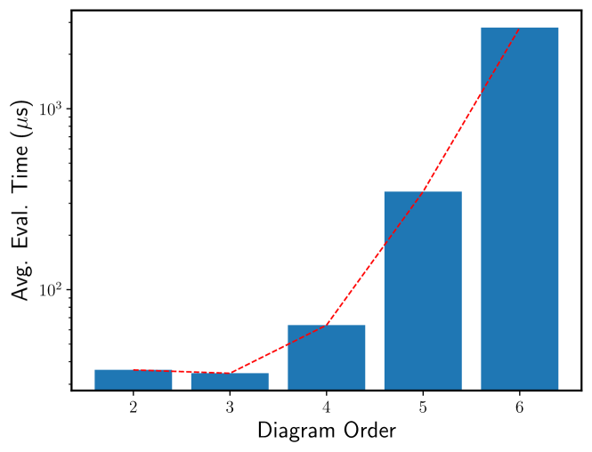
Figure 2: Average time for evaluation (in $\mu$s) per diagram for evaluation in S,P,R format for self-energy diagrams for a random choice of internal parameters on a single modern 3.5 GHz CPU.

6 License and citation policy

The GitHub version of libami is licensed under the GNU General Public License version 3 (GPL v. 3)[18]. We kindly request that the present paper be cited, along with the original algorithmic paper [11], in any published work utilizing an application or code that uses this library.

7 Summary

We have presented a minimal framework for performing symbolic evaluation of Matsubara sums for arbitrary Feynman diagrams. The core of libami is equivalent to a highly optimized symbolic math tool. By avoiding use of generalized symbolic math packages, this AMI library can obtain solutions virtually instantaneously (on the scale of micro-seconds), as demonstrated in Section 5. We have provided example content that should allow users to quickly integrate libami into existing Monte Carlo workflows.

8 Acknowledgments

We acknowledge funding from the Natural Sciences and Engineering Research Council of Canada grant RGPIN-2017-04253.

Appendix A The SPR Evaluation

To implement this procedure we define the following objects:

• The arrays $R_{p}$ representing the configurations of Green’s functions after the $p$th summation (described above).

• The sets of poles $P_{p}$ for $\nu_{p}$ in the configuration of Green’s functions represented by $R_{p-1}$.

• The set of signs $S_{p}$ of the residues for each pole.

The array of poles corresponding to $\nu_{p}$ has entries

$$P_{p}=[P_{p}^{(1)},P_{p}^{(2)},...,P_{p}^{(r_{(p-1)})}],$$ (18)

with each $P_{p}^{(\ell)}$ defined by a set (std::vector) of pole_struct

$$P_{p}^{(\ell)}=[z_{p,\ell}^{(i_{1})},z_{p,\ell}^{(i_{2})},...,z_{p,\ell}^{(i_{r_{\ell}})}].$$ (19)

We note that $P_{p}^{(\ell)}$ is the array of poles for $\nu_{p}$ in the residue of the $\ell$th pole for $\nu_{p-1}$ stored in the previous configuration of Green’s functions, $R_{p-1}$. Similarly, we have an array of signs with the same dimensions as $P_{p}$,

$$S_{p}=[S_{p}^{(1)},S_{p}^{(2)},...,S_{p}^{(r_{(p-1)})}],$$ (20)

with

$$S_{p}^{(\ell)}=[\alpha_{p,\ell}^{(i_{1})},\alpha_{p,\ell}^{(i_{2})},...,\alpha_{p,\ell}^{(i_{r_{\ell}})}],$$ (21)

where $\alpha_{p,\ell}$ are the nonzero coefficients of $\nu_{p}$ from the previous configuration of the Green’s functions, $R_{p-1}$.

Using these arrays, the full analytic result for Eq. (2) is given by

$$I^{(n)}=\frac{1}{\beta^{n}}\sum_{\{\nu_{n}\}}\prod_{j=1}^{N}G^{j}(\epsilon^{j},X^{j}_{m})=K\cdot R_{n},$$ (22)

where

$$K=(S_{1}*f(P_{1}))\times...\times(S_{n}*f(P_{n})).$$

In this expression, $f(P_{p})$ is the Fermi function of an array with elements given by

$$[f(P_{p})]_{\ell}^{i}=f(z_{p,\ell}^{(i)}),$$ (24)

and the operations ‘$*$’, ‘$\times$’, and ‘$\cdot$’ are defined by

$$(C*D)_{i}^{j} = C_{i}^{j}D_{i}^{j}\equiv G_{i}^{j},$$

$$(G\times H)_{i}^{j} = G_{i}H_{i}^{j},$$

$$H\cdot C = \sum_{i}H_{i}C_{i}.$$

Equations (22) and (A) are primary objects of the evaluation stage of AMI.

Appendix B Derivatives of Fermi Functions

We provide a single function fermi_bose($M$,$\sigma$,$\beta$,$E$) to generate the $M$’th derivative of Fermi or Bose functions ($\sigma=+1$ or $-1$, respectively) at inverse temperature $\beta$ and energy $E$. This is generated by a recursive procedure

$$\frac{d^{M}f(E)}{dE^{M}}=(-1)\beta^{M}\sum\limits_{k=0}^{M}F(M,k)\sigma^{k}(-1)^{k+1}$$

$$\times\frac{1}{(\sigma\exp(\beta E)+1)}\frac{1}{(\sigma+\exp(-\beta E))^{k}},$$

where the $F$ function is a combinatorial prefactor. We define the function

$$F(r,k)=\sum\limits_{m=0}^{k}C(k,m)m^{r}(-1)^{k-m},$$ (25)

where C(k,m) is the binomial coefficient.

References

- [1] Amir Taheridehkordi, S. H. Curnoe, and J. P. F. LeBlanc, Algorithmic Matsubara integration for Hubbard-like models, Phys. Rev. B 99 035120 (2019).

References

- [1] G. D. Mahan, Many-particle Physics, 3rd Ed., Springer-Boston MA, 2000.
-
[2]
F. Aryasetiawan, O. Gunnarsson,
TheGWmethod, Reports on
Progress in Physics 61 (3) (1998) 237–312.
doi:10.1088/0034-4885/61/3/002.
URL https://doi.org/10.1088/0034-4885/61/3/002 -
[3]
T. Schäfer, N. Wentzell, F. Šimkovic, Y.-Y.
He, C. Hille, M. Klett, C. J. Eckhardt, B. Arzhang, V. Harkov, F. m. c.-M.
Le Régent, A. Kirsch, Y. Wang, A. J. Kim, E. Kozik, E. A. Stepanov,
A. Kauch, S. Andergassen, P. Hansmann, D. Rohe, Y. M. Vilk, J. P. F. LeBlanc,
S. Zhang, A.-M. S. Tremblay, M. Ferrero, O. Parcollet, A. Georges,
Tracking the
footprints of spin fluctuations: A multimethod, multimessenger study of the
two-dimensional hubbard model, Phys. Rev. X 11 (2021) 011058.
doi:10.1103/PhysRevX.11.011058.
URL https://link.aps.org/doi/10.1103/PhysRevX.11.011058 - [4] M. Jarrell, J. Gubernatis, Bayesian inference and the analytic continuation of imaginary-time quantum monte carlo data, Physics Reports 269 (3) (1996) 133 – 195. doi:https://doi.org/10.1016/0370-1573(95)00074-7.
- [5] R. Levy, J. P. F. LeBlanc, E. Gull, Implementation of the maximum entropy method for analytic continuation, Comp. Phys. Comm. 215 (2017) 149. doi:10.1016/j.cpc.2017.01.018.
-
[6]
M. Shishkin, G. Kresse,
Self-consistent
calculations for semiconductors and insulators, Phys. Rev. B 75 (2007)
235102.
doi:10.1103/PhysRevB.75.235102.
URL https://link.aps.org/doi/10.1103/PhysRevB.75.235102 -
[7]
M. Grumet, P. Liu, M. Kaltak, J. c. v. Klimeš,
G. Kresse, Beyond
the quasiparticle approximation: Fully self-consistent calculations,
Phys. Rev. B 98 (2018) 155143.
doi:10.1103/PhysRevB.98.155143.
URL https://link.aps.org/doi/10.1103/PhysRevB.98.155143 - [8] K. V. Houcke, E. Kozik, N. Prokof’ev, B. Svistunov, Diagrammatic monte carlo, Physics Procedia 6 (2010) 95 – 105. doi:https://doi.org/10.1016/j.phpro.2010.09.034.
-
[9]
R. Rossi,
Determinant
diagrammatic monte carlo algorithm in the thermodynamic limit, Phys. Rev.
Lett. 119 (2017) 045701.
doi:10.1103/PhysRevLett.119.045701.
URL https://link.aps.org/doi/10.1103/PhysRevLett.119.045701 -
[10]
F. Šimkovic, J. P. F. LeBlanc, A. J. Kim,
Y. Deng, N. V. Prokof’ev, B. V. Svistunov, E. Kozik,
Extended
crossover from a fermi liquid to a quasiantiferromagnet in the half-filled 2d
hubbard model, Phys. Rev. Lett. 124 (2020) 017003.
doi:10.1103/PhysRevLett.124.017003.
URL https://link.aps.org/doi/10.1103/PhysRevLett.124.017003 -
[11]
A. Taheridehkordi, S. H. Curnoe, J. P. F. LeBlanc,
Algorithmic
matsubara integration for hubbard-like models, Phys. Rev. B 99 (2019)
035120.
doi:10.1103/PhysRevB.99.035120.
URL https://link.aps.org/doi/10.1103/PhysRevB.99.035120 -
[12]
J. Vučičević,
P. Stipsić, M. Ferrero,
Analytical
solution for time integrals in diagrammatic expansions: Application to
real-frequency diagrammatic monte carlo, Phys. Rev. Research 3 (2021)
023082.
doi:10.1103/PhysRevResearch.3.023082.
URL https://link.aps.org/doi/10.1103/PhysRevResearch.3.023082 -
[13]
R. E. Wengert, A
simple automatic derivative evaluation program, Commun. ACM 7 (8) (1964)
463–464.
doi:10.1145/355586.364791.
URL https://doi-org.qe2a-proxy.mun.ca/10.1145/355586.364791 -
[14]
A. Taheridehkordi, S. H. Curnoe, J. P. F. LeBlanc,
Optimal grouping
of arbitrary diagrammatic expansions via analytic pole structure, Phys. Rev.
B 101 (2020) 125109.
doi:10.1103/PhysRevB.101.125109.
URL https://link.aps.org/doi/10.1103/PhysRevB.101.125109 -
[15]
A. Taheridehkordi, S. H. Curnoe, J. P. F. LeBlanc,
Algorithmic
approach to diagrammatic expansions for real-frequency evaluation of
susceptibility functions, Phys. Rev. B 102 (2020) 045115.
doi:10.1103/PhysRevB.102.045115.
URL https://link.aps.org/doi/10.1103/PhysRevB.102.045115 -
[16]
B. D. E. McNiven, G. T. Andrews, J. P. F. LeBlanc,
Single particle
properties of the two-dimensional hubbard model for real frequencies at weak
coupling: Breakdown of the dyson series for partial self-energy expansions,
Phys. Rev. B 104 (2021) 125114.
doi:10.1103/PhysRevB.104.125114.
URL https://link.aps.org/doi/10.1103/PhysRevB.104.125114 -
[17]
N. Prokof’ev, B. Svistunov,
Bold
diagrammatic monte carlo technique: When the sign problem is welcome, Phys.
Rev. Lett. 99 (2007) 250201.
doi:10.1103/PhysRevLett.99.250201.
URL https://link.aps.org/doi/10.1103/PhysRevLett.99.250201 - [18] Gnu general public license, version 3, http://www.gnu.org/licenses/gpl.html, last retrieved 2020-01-01 (June 2007).