Attosecond dispersion as a diagnostics tool for solid-density laser-generated plasmas

Abstract

Extreme-ultraviolet pulses can propagate through ionised solid-density targets, unlike optical pulses and, thus, have the potential to probe the interior of such plasmas on sub-femtosecond timescales. We present a synthetic diagnostic method for solid-density laser-generated plasmas based on the dispersion of an extreme-ultraviolet attosecond probe pulse, in a pump–probe scheme. We demonstrate the theoretical feasibility of this approach through calculating the dispersion of an extreme-ultraviolet probe pulse propagating through a laser-generated plasma. The plasma dynamics is calculated using a particle-in-cell simulation, whereas the dispersion of the probe is calculated with an external pseudo-spectral wave solver, allowing for high accuracy when calculating the dispersion. The application of this method is illustrated on thin-film plastic and aluminium targets irradiated by a high-intensity pump pulse. By comparing the dispersion of the probe pulse at different delays relative to the pump pulse, it is possible to follow the evolution of the plasma as it disintegrates. The high-frequency end of the dispersion provides information on the line-integrated electron density, whereas lower frequencies are more affected by the highest density encountered along the path of the probe. In addition, the presence of thin-film interference could be used to study the evolution of the plasma surface.

1 Introduction

The interaction between high-intensity lasers and solids has many promising potential applications, such as ion acceleration (Romagnani et al., 2005; Zhang et al., 2017; Higginson et al., 2018), warm-dense-matter generation (Remington et al., 1999; Renaudin et al., 2003; Pérez et al., 2010; Brown et al., 2011), and inertial fusion (Drake, 2018; Le Pape et al., 2018). It is therefore of great importance to further our understanding of these interactions. Insight may be gained through both experiments and numerical simulations, but in order to maximise the utility of the two tools, we must also be able to combine them through experimental diagnostics and comparisons with simulations.

In experiments using solid-density laser-generated plasmas, we have a limited number of experimental diagnostics methods, such as x-ray radiation (Chen et al., 2009; Renner & Rosmej, 2019) or ejected particles (Neely et al., 2006; Nürnberg et al., 2009). In addition to experimental diagnostics, numerical simulations – in particular using the particle-in-cell (PIC) method – are widely used to gain understanding of the evolution of the laser-generated plasma. However, for PIC codes the particle noise is an inherent source of error, and practical limitations on the resolution can lead to unphysical behaviour in certain cases (Juno et al., 2020). In addition, at solid density, especially when the Coulomb logarithm is order unity, the classical two-body treatment of collisions breaks down (Starrett, 2018), thus collision models rely on ad hoc choices and, especially because different choices may lead to significantly different predictions (Sundström et al., 2020b), they need to be validated experimentally. Thus, in order to validate numerical simulations of such high-density laser-generated plasmas, there is a need for additional experimental diagnostics methods that can be used for validation in this density regime.

On the experimental side, there are, for instance, optical probing methods, e.g. shadowgraphy, which have been successful in diagnosing laser-generated plasmas in high detail (Sävert et al., 2015; Siminos et al., 2016). However, optical probing methods are limited to low-density plasmas, typically gas-jet targets, due to the plasma transparency limit. To probe the interior of plasmas at solid density, Kluge et al. (2018) employed the scattering of x-rays from a free-electron laser to study the density evolution in solid density plasma gratings. With the advent of high-harmonic generation (Ferray et al., 1988), attosecond extreme-ultraviolet (XUV) pulses are more readily available to small-scale labs. Furthermore, with reliable methods of generating and measuring XUV pulses (Calegari et al., 2016; Koliyadu et al., 2017), employing XUV frequencies in optical probing methods is now becoming a possibility, for instance, spectral interference methods on the spectral fringes of an attosecond pulse train (Salières et al., 1999; Descamps et al., 2000; Merdji et al., 2000; Hergott et al., 2003), high-harmonic transmission spectroscopy to measure electron density (Hergott et al., 2001; Dobosz et al., 2005), and measurement of XUV refractive index in solid-density plasmas (Williams et al., 2013).

In this paper, we present a method based on the dispersion of an attosecond XUV pulse (or a pulse-train) to diagnose plasmas that are over-dense at optical frequencies. We employ a linearised pseudo-spectral (PS) wave solver to compute the dispersion of the probe pulse for any given plasma profile. In particular, we extract the spatiotemporal plasma profile information along the optical axis from a PIC simulation, through which the probe pulse is propagated separately using the PS solver. The effect of the probe pulse on the plasma evolution is thus neglected. This limitation may be possible to relax if necessary, through a PS fluid modelling of the plasma (Siminos et al., 2014), but because experimentally available XUV intensities are quite low (normalised relativistic amplitudes $a_{1}\lesssim 10^{-3}$), our linearised treatment of the probe pulse is justified. The computed pulse dispersion – our synthetic diagnostic – is most sensitive to the electron density variation across the target, whereas corrections related to the energy distribution of electrons might provide additional constraints at high electron temperatures.

Utilising such modelling in comparison with experimental measurements of the dispersion of the high-frequency pulse across the target, e.g. with the RABBIT (Paul et al., 2001) or attosecond streak-camera (Itatani et al., 2002) methods, could provide an experimental diagnostic. Indeed, this type of experiment have already been performed with (non-ionised) aluminium foil by López-Martens et al. (2005), but not yet in comparison with simulations of the plasma evolution. In addition, the use of isolated attosecond probe pulses in our study provides unprecedented temporal resolution. We note, however, that the use of an isolated pulse is not strictly necessary – although it simplifies the numerical analysis. The main challenge of employing a pulse train, instead of a single pulse, stems from the spectral fringes that it produces, as discussed in § 5.

The structure of this paper is as follows. In § 2 we derive the plasma dispersion for a low-amplitude wave in the presence of relativistic electrons with arbitrary momentum distribution. This is followed in § 3 by a description of a linearised PS wave solver, which allows computation of the group delay of the frequency components in a probe pulse, with minimal numerical dispersion. This tool set is then applied to an output from a PIC simulation in § 4. The results are presented and discussed in § 5 and the conclusions summarised in § 6.

2 Dispersion of the probe pulse

Our goal is to model the propagation of a high-frequency pulse in a laser-generated plasma. Although a PIC code is suitable to model the dynamics of the plasma and the laser pulse used to generate it, there are reasons to model the evolution of the high-frequency probe pulse in an external numerical tool, which is the approach we adopt. Resolving the spatiotemporal scales of the probe within the PIC code would already require excessive numerical resources, while maintaining the accuracy of the phase evolution, such that it is suitable for experimental comparison, in a finite-difference time-domain framework affected by numerical dispersion (Nuter et al., 2014), is simply not feasible (note that even in a non-standard, spectral PIC code with lower numerical dispersion, the extremely high resolution requirement would still persist; there may also be potential issues with the level of discretisation noise compared with the probe pulse amplitude.)

In the following, we derive the plasma response to a spatial harmonic of the probe pulse, in the presence of electrons with arbitrary momentum distribution $f({\bf\it p})$. The resulting expression is then used in the numerical framework, external to the PIC code, to evolve the probe pulse based on the plasma information obtained from the PIC simulation, described in § 3.

We treat the probe pulse as a ray propagating along a line in the plasma, assuming negligible plasma variations over the transverse extent of the probe pulse, thereby keeping the formalism one-dimensional (1D). Consider a transverse electromagnetic wave, described by its vector potential ${\bf\it A}_{\perp}$. In a 1D geometry, conservation of transverse canonical momentum dictates that the momentum response of the electrons is ${\bf\it p}_{\perp}=e{\bf\it A}_{\perp}$, where $-e$ is the electron charge. In a cold-fluid plasma, assuming stationary ions, the corresponding current response is

$${\bf\it j}_{\perp}=-en_{\mathrm{e}}{\bf\it v}_{\mathrm{e},\perp}=-\frac{e^{2}n_{\mathrm{e}}{\bf\it A}_{\perp}}{\gamma_{\mathrm{e}}m_{\mathrm{e}}},$$ (1)

where $n_{\mathrm{e}}$ is the electron density, ${\bf\it v}_{\perp}={\bf\it p}_{\perp}/m_{\mathrm{e}}\gamma_{\mathrm{e}}$ is the fluid velocity of the electrons, $m_{\mathrm{e}}$ is the electron mass, and $\gamma_{\mathrm{e}}$ is the Lorentz factor of the electron fluid motion. We can now write down the 1D wave equation for a cold-fluid plasma as

$$\partialderivative[2]{{\bf\it A}_{\perp}}{t}-c^{2}\partialderivative[2]{{\bf\it A}_{\perp}}{x}=c^{2}\mu_{0}{\bf\it j}_{\perp}=-\frac{\omega_{\mathrm{p}}^{2}}{\gamma_{\mathrm{e}}}{\bf\it A}_{\perp},$$ (2)

where the wave is propagating along the $x$ direction, $c$ is the speed of light in vacuum, and

$$\omega_{\mathrm{p}}^{2}\equiv\frac{e^{2}n_{\mathrm{e}}}{\epsilon_{0}m_{\mathrm{e}}}$$ (3)

defines the non-relativistic plasma frequency $\omega_{\mathrm{p}}$.

For a low-amplitude wave, such as the high-harmonic generated pulses available today, $a_{1}=eA_{1}/(m_{\mathrm{e}}c)\ll 1$ where $A_{1}$ is the amplitude of the wave vector potential, we may neglect the contribution from the wave-induced oscillation to the Lorentz factor $\gamma_{\mathrm{e}}$. For the moment, we also assume that the longitudinal fluid momentum of the electrons is small, $p_{x}\ll m_{\mathrm{e}}c$, such that $\gamma_{\mathrm{e}}\simeq 1$. Thus, the prefactor on the-right hand side of (2) is independent of ${\bf\it A}_{\perp}$, and we recover the cold-plasma dispersion relation $c^{2}k^{2}=\omega^{2}-\omega_{\mathrm{p}}^{2}$.

Note that in this derivation we have neglected effects of particle collisions, which, if sufficiently strong, could affect both the phase shifts and damping of the wave. In the cases considered in this paper, however, we estimate the electron–ion collision frequencies $\nu_{\mathrm{e}\mathrm{i}}$ to be one to two orders of magnitude lower than the XUV probe frequencies – owing to the approximately kiloelectronvolt electron temperatures reached – and can therefore be neglected (note that collisional corrections to phase delays are quadratic in $\nu_{\mathrm{e}\mathrm{i}}/\omega\ll 1$). In cases where collisions play a larger role, e.g. in colder plasmas, the wave equation (2) could be modified to accommodate collisional effects via a damping term $\tilde{\nu}\partialderivative*{{\bf\it A}_{\perp}}{t}$ (added to the left-hand side), where $\tilde{\nu}$ is an effective damping rate due to collisions. Finding an appropriate expression for $\tilde{\nu}$ is non-trivial, but once that is done, the PS solver outlined in § 3 is easily modified to include this damping term.

2.1 Relativistic birefringence: a kinetic correction to the plasma frequency

In the above presentation, we used a cold-fluid description of the plasma response to the electromagnetic wave. In reality, the electrons are not cold, and relativistic effects will require a modification to the current response of an individual electron based on its initial momentum, as was pointed out by Stark et al. (2015) and further developed by Arefiev et al. (2020). In general, the Lorentz factor contributes to increasing the inertia of the electrons, which lowers the effective plasma frequency. This effect is akin to relativistic transparency (Kaw & Dawson, 1970; Siminos et al., 2012), but here it is the general effect of relativistic plasmas – not just the relativistic electron motion induced by the laser. In this subsection, we present the relativistic, kinetic correction to the plasma frequency for a low-amplitude wave.

For an electron subject to a field with vector potential ${\bf\it A}_{\perp}=A_{y}\hat{{\bf\it y}}$, its corresponding change in momentum would be $\delta{p_{y}}=eA_{y}$ due to conservation of transverse canonical momentum. Importantly, this change in momentum is independent of the initial momentum of the electron. However, the velocity response – and thus also the current response – does depend on the initial momentum. Therefore, when calculating the velocity response, we must consider the initial Lorentz factor of the electron, $\gamma=(1+p_{x}^{2}+p_{y}^{2}+p_{z}^{2})^{1/2}$. Here, and in the rest of this subsection, we use the normalisation $m_{\mathrm{e}}=1=c$, unless stated otherwise.

Small wave amplitudes allow linearisation of the change in velocity ${\bf\it v}={\bf\it p}/\gamma$ due to the small momentum perturbation $\delta{p_{y}}$ in the $y$ direction (polarisation direction). The corresponding change in velocity can be expressed as

$$\delta{v_{y}}\approx\delta{p_{y}}\derivative{v_{y}}{p_{y}}=\delta{p_{y}}\quantity(\partialderivative{v_{y}}{p_{y}}+\partialderivative{v_{y}}{\gamma}\partialderivative{\gamma}{p_{y}})=\frac{\delta{p_{y}}}{\gamma}\quantity(1-\frac{p_{y}^{2}}{\gamma^{2}}).$$ (4)

From this expression, we can note that the corresponding change in velocity depends on the initial momentum and the respective direction of the momentum perturbation.

Next, we obtain the full current response of the plasma by integrating the individual velocity response $\delta{v_{y}}$ over the electron distribution function $f$,

$$\delta{j}_{y}=-e\int\!\differential[3]{p}\,\delta{v_{y}}f({\bf\it p})=-e\,\delta{p_{y}}\int\!\differential[3]{p}\frac{f({\bf\it p})}{\gamma}\quantity(1-\frac{p_{y}^{2}}{\gamma^{2}}).$$ (5)

In particular, we may lift the momentum perturbation $\delta{p}_{y}=eA_{y}$ outside the integral because the conservation of canonical momentum applies to each electron, regardless of its initial momentum. In the previous calculations, we have used $\hat{{\bf\it y}}$ as the direction of polarisation ${\bf\it A}_{\perp}=A_{y}\hat{{\bf\it y}}$, but the same calculations can easily be extended to an arbitrary polarisation direction $\hat{{\bf\it e}}$, by replacing all instances of $p_{y}$ with ${\bf\it p}\dotproduct\hat{{\bf\it e}}$.

Finally, we note that we can obtain the kinetically corrected dispersion relation by replacing the non-relativistic plasma frequency (3) with a relativistic plasma frequency

$$\tilde{\omega}_{\mathrm{p},\hat{{\bf\it e}}}^{2}=\frac{e^{2}}{\epsilon_{0}m_{\mathrm{e}}}\int\!\differential[3]{p}\frac{f({\bf\it p})}{\gamma}\quantity(1-\frac{({\bf\it p}\dotproduct\hat{{\bf\it e}})^{2}}{\gamma^{2}})=\frac{e^{2}n_{\mathrm{e}}}{\epsilon_{0}\tilde{\gamma}_{\hat{{\bf\it e}}}m_{\mathrm{e}}},$$ (6)

where $m_{\mathrm{e}}$ has been added back to the prefactor for clarity. The relativistic plasma frequency can then simply be used in the plasma-response term in the wave equation (2). In the last step, we also introduced an effective gamma factor, defined by

$$\tilde{\gamma}^{-1}_{\hat{{\bf\it e}}}\equiv\frac{1}{n_{\mathrm{e}}}\int\!\differential[3]{p}\frac{f({\bf\it p})}{\gamma}\quantity(1-\frac{({\bf\it p}\dotproduct\hat{{\bf\it e}})^{2}}{\gamma^{2}}).$$ (7)

The effective gamma factor corresponds to the relative difference between the relativistic and non-relativistic plasma frequencies, $\tilde{\gamma}^{-1}_{\hat{{\bf\it e}}}=\tilde{\omega}_{\mathrm{p},\hat{{\bf\it e}}}^{2}/\omega_{\mathrm{p}}^{2}$. If the distribution is not isotropic, then $\tilde{\gamma}_{\hat{{\bf\it e}}}$ – and thereby $\tilde{\omega}_{\mathrm{p},\hat{{\bf\it e}}}^{2}$ – are polarisation dependent, hence we can talk about this effect as a “relativistic birefringence”.

For thermal distributions at temperatures below approximately $10{\rm\,keV}$, we show in Appendix A, that the relative reduction of the plasma frequency due to the effective gamma factor is only of the order of a few per cent. Therefore, in most experimentally relevant cases, the attosecond dispersion can be said to probe the electron density.

3 Linearized pseudo-spectral wave solver

A spectral solver is based on discretising and evolving the wave spectrum rather than the real-space wave. The main benefit of a spectral solver is that numerical dispersion can be reduced drastically compared with spatial discretisations, such as the commonly used Yee mesh. Although numerical dispersion in the context of PIC codes (Nuter et al., 2014) is often discussed with respect to numerical Cherenkov radiation (Godfrey, 1974), it can also greatly affect the accuracy of the evolution of the electromagnetic wave, which is the main problem addressed here.

In a periodic domain of length $L$, we may Fourier decompose the wave vector potential in space into spectral modes,

$${\bf\it A}_{\perp}(x;t)=\sum_{k}{\bf\it\hat{A}}_{\perp,k}(t)\,\mathrm{e}^{\mathrm{i}kx},$$ (8)

where the sum is over all integer multiples of $\rmDelta{k}=2\upi/L$; once the domain has been discretised into $N$ equally spaced points, the upper and lower limit to the sum are $\pm N\rmDelta{k}/2=\pm N\upi/L$. We may also transform $\tilde{\omega}_{\mathrm{p}}^{2}(x;t)\mapsto\hat{\omega}_{\mathrm{p},k}^{2}(t)$ analogously. Through this Fourier decomposition, we can replace the spatial derivatives $\partialderivative*{x}\mapsto\mathrm{i}{k}$, and the wave equation (2) now becomes

$$\partialderivative[2]{{\bf\it\hat{A}}_{\perp,k}}{t}+c^{2}k^{2}{\bf\it\hat{A}}_{\perp,k}=-\sum_{k^{\prime}}\hat{\omega}_{\mathrm{p},k^{\prime}}^{2}{\bf\it\hat{A}}_{\perp,(k-k^{\prime})}.$$ (9)

It has been reduced to a set of coupled ordinary differential equations, which can be solved using standard methods, e.g. Runge–Kutta. The right-hand side of (9) is a convolution in $k$ space (according to the Convolution theorem of Fourier analysis) which can be evaluated efficiently using a PS approach, i.e. it is transformed back to real space in each time step, where this convolution is reduced to a multiplication. This is particularly convenient as $\tilde{\omega}_{\mathrm{p}}^{2}(x;t)$ is provided in real space from the simulations.

In this method, we have implicitly assumed a periodic domain. For the purposes of this paper – to study the dispersion of an XUV pulse through a foil-target laser-generated plasma – the simulation can be accommodated in such a periodic domain by allowing for sufficiently large vacuum regions on both sides of the laser-generated plasma. In such a simulation, there is no need for the XUV pulse to cross the periodic boundary. Other types of simulations, where the plasma extends the full length of the simulation box and where the XUV pulse propagates though the periodic boundary can also be accommodated, as long as the XUV pulse does not cross the boundary of the plasma simulation – e.g. by projecting a moving window plasma-simulation domain onto the PS periodic domain.

Finally, we note that the numerical methods for solving the second-order differential equation usually involves decomposing the time derivative into two first-order derivatives. By doing so, we obtain the electric field ${\bf\it{\bf\it E}}=-\partialderivative*{{\bf\it A}}{t}$ – which is the quantity that can be measured in experiments – essentially ‘for free’.

3.1 Calculating phase shifts

The main result that we seek from the PS computation is the dispersion or relative phase shifts of the frequency components of the XUV pulse, which can be measured experimentally. Although the phase $\phi_{k}(t)$ is encoded in the Fourier spectrum as the complex phase of

$$\hat{E}_{k}(t)=\absolutevalue*{\hat{E}_{k}(t)}\mathrm{e}^{\mathrm{i}\phi_{k}(t)}\equiv\absolutevalue*{\hat{E}_{k}(t)}P_{k}(t),$$ (10)

it is not trivial to recover $\phi_{k}(t)$ from $P_{k}(t)$, because $P_{k}(t)$ only contains phase information modulo $2\pi$. Practically, this makes it nearly impossible to reconstruct the relative phases of two frequency components separated by more than a few steps in the discretised $k$ space.

Instead of analysing $P_{k}$ directly, we may use $\bar{P}_{k}(t)\equiv P_{k}(t)\mathrm{e}^{\mathrm{i}{}\omega_{k}t}=\mathrm{e}^{\mathrm{i}[\phi_{k}(t)+ckt]}=\mathrm{e}^{\mathrm{i}\bar{\phi}_{k}(t)}$, which will make the phase-shift analysis clearer. This view removes the relative phase shifts due to vacuum propagation, and is equivalent to studying the pulse in a comoving window that moves with the speed of light. Any phase shifts observed in this frame is therefore due to the plasma dispersing the pulse.

As the full information of the relative phase shifts is difficult to extract directly from the complex spectral phase $\bar{P}_{k}$, some other method is necessary. Fortunately, because we are interested in the relative phases, we can study the change of $\bar{P}_{k}$,

$$\rmDelta\bar{P}_{k}={} \bar{P}_{k+1}-\bar{P}_{k}=\mathrm{e}^{\mathrm{i}\bar{\phi}_{k+\rmDelta{k}}}-\mathrm{e}^{\mathrm{i}\bar{\phi}_{k}}=\mathrm{e}^{\mathrm{i}\bar{\phi}_{k}}\big{[}\mathrm{e}^{\mathrm{i}\rmDelta\bar{\phi}_{k}}-1\big{]}$$ (11)

$$={} \bar{P}_{k}\;\quantity[\mathrm{i}\sin(\rmDelta\bar{\phi}_{k})+\cos(\rmDelta\bar{\phi}_{k})-1],$$

where the phase variation is $\rmDelta\bar{\phi}_{k}=\bar{\phi}_{k+\rmDelta{k}}-\bar{\phi}_{k}$. From (11), we can define a related phase-rate variable

$$\bar{\psi}_{k}\equiv-\frac{\mathrm{i}\rmDelta\bar{P}_{k}}{\bar{P}_{k}}=\sin(\rmDelta\bar{\phi}_{k})+\mathrm{i}\quantity[1-\cos(\rmDelta\bar{\phi}_{k})].$$ (12)

This variable is still $2\pi$ periodic, but now the periodicity is in $\rmDelta{\bar{\phi}_{k}}$, which is smaller than the $\pm\pi$ window of retrievable information – provided that the spectral resolution $N$ is sufficiently large. We can, therefore, retrieve $\rmDelta\bar{\phi}_{k}$, with which the properly unwrapped phase $\phi_{k}$ can be reconstructed, up to a constant phase shift.

In an experiment, however, it is the relative group delay of the different frequency components that is measured. The group delay $\tau$ is defined as the rate of phase change, which, in the discrete case, we approximate as

$$\tau\equiv\partialderivative{\phi}{\omega}\approx\frac{\rmDelta\phi_{k}}{\rmDelta\omega}=\frac{\rmDelta\phi_{k}}{c\rmDelta{k}}\equiv\tau_{k}.$$ (13)

With this, we now have a full tool set for computing the relative group delay of a low-amplitude probe pulse in any given 1D plasma profile $\tilde{\omega}_{\mathrm{p}}^{2}(x;t)$, with minimal numerical dispersion. This tool set can be applied on the output form a PIC simulation to create a synthetic diagnostic for a laser-generated plasma experiment.

4 PIC and PS simulations

The workflow for generating the synthetic dispersion diagnostic consists of two main components: first the PIC simulation to simulate the plasma evolution due to the pump laser pulse, then the PS method is used to calculate the dispersion of the probe pulse as it propagates through the plasma profile generated by the PIC simulation. This two-step process works for sufficiently low-amplitude probe pulses, where the effects of the probe pulse on the plasma are negligible.

4.1 PIC simulation parameters

We used the PIC code Smilei (Derouillat et al., 2018), to generate on-axis profiles of the relativistic plasma frequency $\tilde{\omega}_{\mathrm{p}}^{2}(x;t)$ from (6), which could then be used in the linearised PS wave solver. To this end, we performed two-dimensional (2D), fully collisional (Pérez et al., 2012), PIC simulations of a thin plastic foil target irradiated by a circularly polarised pump pulse with wavelength $\lambda_{0}=800{\rm\,nm}$, peak intensity $1.9{\times}10^{19}{\rm\,W\,cm^{-2}}$ (normalised amplitude $a_{0}=3.0$). The pulse temporal and spatial profiles were both Gaussian with intensity full-width-at-half-maximum (FWHM) duration of $30{\rm\,fs}$ and spot size (waist diameter) of $6{\rm\,\text{\textmu}{m}}$.

The thin-foil plasma studied here has a trapezoidal density profile with a $0.25{\rm\,\text{\textmu}{m}}$ plateau and $25{\rm\,nm}$ linear density ramps on both sides, fully ionised, solid-density polyethylene ($\rm CH_{2}$), corresponding to an initial electron density of $n_{0,\mathrm{e}}=177.7\,n_{\rm c,0}=3.1{\times}10^{23}{\rm\,cm^{-3}}$, where $n_{\rm c,0}=\epsilon_{0}m_{\mathrm{e}}\omega_{0}^{2}/e^{2}$ is the critical density associated with the pump laser frequency $\omega_{0}$. The plasma was modelled with 120, 30 and 15 macro-particles per cell for the electrons, protons and carbon ions, respectively.

The simulation box was $10{\rm\,\text{\textmu}{m}}$ and $20{\rm\,\text{\textmu}{m}}$ in the $x$ and $y$ directions, respectively, with $4096$ cells in each direction, giving a spatial resolution of $\rmDelta{x}_{\rm PIC}=2.44{\rm\,nm}$ and $\rmDelta{y}_{\rm PIC}=4.88{\rm\,nm}$. The target front edge lies at $x=4.5{\rm\,\text{\textmu}{m}}$ from the left edge of the box. Peak on-target intensity occurs at simulation time $t=78.6{\rm\,fs}$. The simulations output a binned quantity corresponding to the relativistic plasma frequency squared $\tilde{\omega}^{2}_{\mathrm{p},\hat{{\bf\it y}}}$ (6). In these simulations, $\tilde{\omega}^{2}_{\mathrm{p},\hat{{\bf\it y}}}$ is around $1\,\%$ lower than the non-relativistic plasma frequency squared (3). Particles within $\pm 0.5{\rm\,\text{\textmu}{m}}$ from the optical axis were used in the binning, to create the plasma profile used by the PS solver. The longitudinal resolution of the binning was the same as the cell length.

We have chosen the target and laser parameters to illustrate one possible application of the XUV dispersion diagnostics: time-resolving the disintegration of a thin foil when irradiated by the pump pulse. As the electrons are energised by the pump laser, they escape from both the front and back end of the target, which decreases the density on axis. Therefore, by varying a delay between the probe and the pump pulse, the different densities can be inferred from the decrease in dispersion.

As a comparison with the plastic target, we also performed a similar simulation of a $0.1{\rm\,\text{\textmu}{m}}$ thin aluminium foil, with $10{\rm\,nm}$ linear density ramps on each side. The aluminium is taken to be fully ionised at solid density, corresponding to an initial electron density of $n_{0,\mathrm{e}}=449.4\,n_{\rm c,0}=7.8{\times}10^{23}{\rm\,cm^{-3}}$, which is very close to $2.5$ times that of the plastic target. The plasma was modelled with 120 and 40 particles per cell for the electrons and aluminium ions, respectively. The other parameters were kept the same as for the plastic target. The comparison with the thicker plastic target is interesting because the initial integrated density, along the optical axis, is the same between the two targets.

4.2 PS simulation parameters

The plasma profiles generated in the PIC simulations are used in the PS solver to accurately and efficiently calculate the dispersion of the probe pulse. Note that the solver takes both spatial and temporal variation into account. In order to get the desired resolution, the PIC output is interpolated in both time and space.

Because of the good numerical accuracy of a spectral solver, the resolution does not have to be much greater than what was used in the PIC simulation. The whole length $L_{x}=10{\rm\,\text{\textmu}{m}}$ of the PIC-simulation box was discretised with $N=8196$ points (twice that of the PIC simulation), corresponding to a resolution of $\rmDelta{x}_{\rm PS}=1.22{\rm\,nm}$. This discretisation allows for a maximum wavenumber of $k_{\max}=\pi N/L_{x}=2.57{\rm\,nm^{-1}}$ (corresponding to a minimum resolved wavelength of $2\rmDelta{x}_{\rm PS}=2.44{\rm\,nm}$) with a wavenumber resolution of $\rmDelta{k}=2\pi/L_{x}=6.28\times 10^{-4}{\rm\,nm^{-1}}$. The time resolution was automatically handled in the Runge–Kutta method implemented in the function solve_ivp from SciPy version 1.6.3 (Jones et al., 2001–). In Appendix B, we present some benchmarks of the PS code.

The probe pulse electric field is initialised in real space in the vacuum region near the front of the target. The initial pulse shape has a four-cycle-duration $\cos^{2}$ envelope on a centred sinusoidal carrier wave. The central wavelength is $\lambda_{1}=30{\rm\,nm}$ corresponding to a wavenumber of $k_{1}=0.21{\rm\,nm^{-1}}$. Note, however, that the shape of the initial pulse is not very important to the dispersion measurement. The pump–probe delay is set by a temporal shift of the $\tilde{\omega}_{\mathrm{p}}^{2}(x;t)$ profiles from the PIC simulation. When analysing a spectrum from the simulation, it is important that the whole pulse is in vacuum, so that the wavenumber and the frequency spectra are the same. Otherwise, distortions of the spectrum due to the plasma dispersion makes comparisons of spectral data difficult.

With the carrier wavelengths above, the initial target electron densities correspond to $n_{0,\mathrm{e}}\approx 0.25\,n_{\rm c,1}$ and $\approx 0.6\,n_{\rm c,1}$ for the plastic and aluminium targets, respectively, where $n_{\rm c,1}$ is the critical density for the central frequency $\omega_{1}=ck_{1}$ of the probe pulse. As these values are close to unity, there will be a significant portion of the pulse that is reflected. Because the reflected part propagates in the opposite direction, it has a very strong influence on the phase information of the spectrum. It is, therefore, important to filter out the reflected pulse, and only study the spectrum of the transmitted part of the pulse. This filtering is most readily done in real space.

As the PS solver evolves each wavenumber component independently, the group delay incurred for each $k$ component is, in principle, not affected by the initial pulse shape. (There may be some minor effects due to the timing of each component in relation to the plasma evolution, but they would be in order of the ratio of plasma-evolution rate to pulse duration.) However, the initial pulse shape has one important effect on the dispersion analysis. That is the initial relative group delays. With the choice of a symmetric envelope and symmetric carrier phase, each wavenumber component will have the same vacuum-propagation-corrected spectral phase $\bar{P}_{k}=0$, i.e. there are no relative group delays in such a pulse. Conversely, if some other probe-pulse shape is used, the observed group delays will be affected by the initial spectral phases of the pulse. For the purposes of a synthetic diagnostic to an experiment, however, one could use the same pulse shape as used in the experiment; the resulting group delay information can then be compared directly with observations.

5 Results and discussion

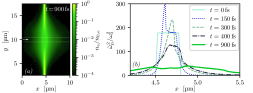
Figure 1: (a) Electron density in the polyethylene plasma at $t=900{\rm\,fs}$; peak on-target pump intensity occurs at $t\approx 80{\rm\,fs}$. (b) Profiles of the squared relativistic plasma frequency $\tilde{\omega}_{\mathrm{p}}^{2}$, relative to the squared pump-laser central frequency $\omega_{0}^{2}$, along the optical axis (white arrow in panel a), for $t=0{\rm\,fs}$ (solid line), $t=150{\rm\,fs}$ (dotted line), $t=300{\rm\,fs}$ (dashed line), $t=400{\rm\,fs}$ (dash-dotted line), and $t=900{\rm\,fs}$ (thick solid line). The profiles are created by averaging (in $y$) across a band $\pm 0.5{\rm\,\text{\textmu}{m}}$ from the optical axis (thin dotted lines in panel a).

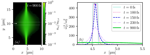
Figure 2: (a) Electron density in the aluminium plasma at $t=900{\rm\,fs}$; peak on-target pump intensity occurs at $t\approx 80{\rm\,fs}$. (b) Profiles of the squared relativistic plasma frequency $\tilde{\omega}_{\mathrm{p}}^{2}$, relative to the squared pump-laser central frequency $\omega_{0}^{2}$, along the optical axis (white arrow in panel a), for $t=0{\rm\,fs}$ (solid line), $t=100{\rm\,fs}$ (dotted line), $t=150{\rm\,fs}$ (dashed line), $t=230{\rm\,fs}$ (dash-dotted line), and $t=900{\rm\,fs}$ (thick solid line). The profiles are created by averaging (in $y$) across a band $\pm 0.5{\rm\,\text{\textmu}{m}}$ from the optical axis (thin dotted lines in panel a).

With such thin foils, the targets rapidly disintegrate due to hydrodynamical expansion after irradiation by the pump pulse. Figure 1(a) shows an electron-density map, from the plastic target, at the simulation time $t=900{\rm\,fs}$, approximately $820{\rm\,fs}$ after peak on-target pump intensity. In the figure, we see how the electrons have expanded out in plumes, both in front of and behind the target. Figure 1(b) shows the on-axis squared relativistic plasma frequency $\tilde{\omega}_{\mathrm{p}}^{2}$, given by (6), for four different time steps of the simulation. Note that $\tilde{\omega}_{\mathrm{p}}^{2}$ is approximately proportional to $n_{\mathrm{e}}$. It is these profiles that are being probed by the XUV pulse, which passes through the plasma along the optical axis $y=10{\rm\,\text{\textmu}{m}}$ (white arrow in fig. 1a); the $\tilde{\omega}_{\mathrm{p}}^{2}$ values are averaged across $\pm 0.5{\rm\,\text{\textmu}{m}}$ in $y$ on each side of the axis (thin dotted lines in fig. 1a).

In the evolution of the plasma, it is initially compressed ($t=150{\rm\,fs}$, dotted line) by the pump pulse, creating a density spike at the front. As the electrons are rapidly heated to kiloelectronvolt temperatures, the plasma starts to expand and expansion fronts (the interface between the perturbed and unperturbed plasma) propagate inwards from both ends of the target and meet in the middle. As the expansion fronts collide, at first a narrow density peak is created ($t=300{\rm\,fs}$, dashed line), but that peak is rapidly flattened as material is continuously escaping on both sides ($t=400{\rm\,fs}$, dash-dotted line). Finally, the plasma continues to expand, which results in a lower but elongated plasma profile ($t=900{\rm\,fs}$, thick green solid line, corresponding to the density map in fig. 1a).

A similar evolution is observed in the simulation with the aluminium foil target. Figure 2(a) shows an electron-density map at $t=900{\rm\,fs}$ (same as the corresponding density map in fig. 1a). The plasma profiles in fig. 2(b) (averaged across $\pm 0.5{\rm\,\text{\textmu}{m}}$ on each side of the optical axis, white dotted lines in fig. 2a) show the same general steps in the evolution of the aluminium plasma as in the plastic-target plasma. Although the initial laser compression in the aluminium plasma is essentially non-existent ($t=100{\rm\,fs}$, dotted line), there is still the interaction of the two expansion fronts. At $t=150{\rm\,fs}$, the expansion fronts meet in the middle, which creates at sharp peak (dashed line). Then, as the electrons continue to escape, the peak is flattened ($t=230{\rm\,fs}$, dash-dotted line).

From both fig. 1(a) and 2(a), we see that the transverse variations occur on length scales on the order of micrometres. Therefore, the transverse beam profile of the probe pulse should be smaller than that for the 1D assumption in the PS computation of the probe-pulse dispersion to hold. Coudert-Alteirac et al. (2017) demonstrated an XUV spot size of ${\simeq}4{\rm\,\text{\textmu}{m}}$, which is slightly larger than what would be ideal for the cases studied here. More recently, Major et al. (2021) demonstrated a tightly focused waist (diameter) of $\simeq 0.7{\rm\,\text{\textmu}{m}}$. However, the probe beam cannot be too tightly focused for the 1D assumption to hold either. Thus, to avoid the 1D treatment from breaking down, the best option would be to study plasmas generated by a wider pump pulse, so that the transverse variations can accommodate a several-micrometer-wide XUV probe pulse.

Another possibility to handle transverse plasma variations is to extend the numerical treatment in the PS solver to two or three dimensions. Although, the conceptual steps to extend the algorithm to higher dimensions are simple, some additional complexity arises. The periodic boundary conditions in the transverse directions – caused by the spectral treatment – would have to be handled carefully. In addition, as the pulse would be dispersed differently in the transverse plane, the analysis of the arising range of group delays need to involve a more accurate model of the experimental setup and detection in the RABBIT or streak-camera methods. We have, therefore, limited the scope of this study to a 1D dispersion analysis.

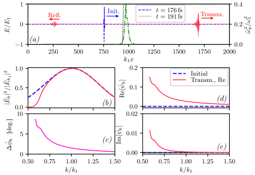
Figure 3: Overview of the PS output for the baseline 2D PIC simulation, where the XUV probe pulse is $100\rm\,fs$ delayed after the pump. (a) Real-space representation of the probe pulse (blue and red lines) and the plasma profile at the final time (green dotted line; right axis). The dotted line represents a spatial filter used on the reflected part of the pulse when computing the transmitted spectra. (b) Initial (dashed line) and transmitted (solid line) spectral intensity $|\hat{E}_{k}|^{2}/|\hat{E}_{k_{1}}|^{2}$ of the probe pulse normalised to the maximum value at the central wavenumber $k_{1}$. (c) Phase variation $\rmDelta\bar{\phi}_{k}$ of the transmitted pulse. (d) Real and (e) imaginary part of the phase-rate variable $\bar{\psi}_{k}$ for the transmitted (solid line) and the initial (dashed line) probe pulse.

With plasma profiles from a PIC simulation, the attosecond probe pulse dispersion can now be calculated using the PS wave solver. Figure 3 shows an overview of the information obtained by such a PS computation, in this case with the plastic target. In fig. 3(a), the normalised real-space waveforms of the initial probe pulse at $k_{1}x=750$ (dashed blue line) and the final waveform of the transmitted and reflected parts of the pulse (solid red line), at $k_{1}x\approx 1700$ and $k_{1}x\approx 250$, respectively. We clearly see that the transmitted part of the pulse is significantly wider than the initial pulse, showing that the pulse has been dispersed. The reflected pulse is discarded from the later spectral analysis, via a spatial filter on the real-space waveforms (represented as the black dashed line in fig. 3a). The plasma profile ($t=191{\rm\,fs}$) which the pulse passes through is shown on the right axis relative to the probe central frequency $\tilde{\omega}_{\mathrm{p}}^{2}/\omega_{1}^{2}$ (dash-dotted green line).

Figure 3(b) shows the normalised energy spectral density $|\hat{E}_{k}|^{2}/|\hat{E}_{k_{1}}|^{2}$ of the initial (dashed blue line) and transmitted (solid red line) probe pulse. There is a clear cutoff in the transmitted spectrum at slightly above the initial plasma frequency of $\tilde{\omega}_{\mathrm{p},0}=0.50\,\omega_{1}$. This is expected, since bulk of the plasma is still at its initial density, making it over-dense for frequencies less than $\tilde{\omega}_{\mathrm{p},0}=0.50\,\omega_{1}$.

The dispersion of the probe pulse is encoded in the spectral phase information, which can be retrieved using the methods discussed in § 3.1. Figures 3(d & e) show the real and imaginary parts, respectively, of the phase-rate variable $\bar{\psi}_{k}$ for the transmitted pulse as well as the initial pulse. We see that $\real(\bar{\psi}_{k})=\sin(\rmDelta\bar{\phi}_{k})$ increases as $k$ approaches the cutoff near $k\simeq 0.6\,k_{1}$, which is expected as the group velocity decreases for frequencies closer to the plasma frequency. Note that the flat initial value of $\bar{\psi}_{k}=0$ is due to the choice of initial pulse shape; see § 4.2 for a short discussion on the effects of the initial pulse shape. From $\bar{\psi}_{k}$, we reconstruct the phase variation $\rmDelta\bar{\phi}_{k}$ (fig. 3d) that is proportional to the group delay, which is what would be measured with the attosecond streak-camera (Itatani et al., 2002) method in an experiment.

We have employed an isolated attosecond pulse for the dispersion analysis in this paper, which somewhat simplifies the computation and analysis of the group delays. However, it is experimentally more challenging to generate such isolated attosecond pulses compared to trains of attosecond pulses. The PS solver and the methods used for computing the group delays are general and, thus, capable of handling any waveform – including pulse train. However, handling the fringes in the spectra caused by pulse trains requires some care when analysing the group-delay data. Only the group delays at each spectral maxima should be considered; this corresponds to the information gathered using the RABBIT (Paul et al., 2001) method. Furthermore, the plasma processes considered in this paper occur on approximately $1{-}10{\rm\,fs}$ time scales, which means that the sub-femtosecond temporal resolution provided by an isolated attosecond pulse is not strictly necessary.

5.1 Diagnosing plasma evolution

Using the group delay as a tool, we can now diagnose the plasma evolution in the PIC simulations by comparing the group delay for different pump–probe delays. Figure 4(a) shows the relative group delay curves $\tau_{k}$ obtained from the plastic plasma, at four different pump–probe delays $t_{1}$, where $t_{1}$ is measured between the peak intensities of the pump and probe pulses. The $\tau_{k}$ curves are plotted in the wavenumber range where the spectral intensity $|\hat{E}_{k}|^{2}/|\hat{E}_{k_{1}}|^{2}>0.05$ is greater than 5% of that of the central frequency, to remove the experimentally not measurable regions. We see that the slope of the $\tau_{k}$ curves decreases as the pump–probe delay is increased, which means that the dispersion of the probe pulse decreases. The lowered dispersion is a sign that the bulk $\tilde{\omega}_{\mathrm{p}}^{2}$ decreases with time, as one would expect from a disintegrating plasma and indeed is observed in fig. 1(b). We also note that even if the plasma were to expand one-dimensionally, i.e. having a constant line-integrated density, the $\tau_{k}$ curves would still be different as changes in the maximum density would translate to shifts in the cutoff frequency.

Another interesting feature seen in fig. 4(a) is the oscillation in $\tau_{k}$ for $t_{1}=0{\rm\,fs}$ (and a few very weak oscillations for $t_{1}=100{\rm\,fs}$). These oscillations occur due to internal reflections inside the intact target. The XUV pulse is reflected against the sharp plasma–vacuum boundaries several times, thus generating a train of very low-intensity pulses following the main transmitted pulse, which generates interference – much like thin-film interference. The interference pattern can also be seen as spectral fringes in the intensity spectrum, shown in fig. 4(c). The reason why the interference patterns do not appear at longer pump–probe delays $t_{1}\gtrsim 100{\rm\,fs}$ is due to the destruction of the sharp plasma–vacuum boundaries as the plasma expands. This is interesting, because the presence of thin-film interference in an XUV probe could be used to study the evolution of the plasma surface, given that a sufficiently high-contrast pump pulse is used. Furthermore, the spacing of the fringes can give some information about the plasma thickness. Note, however, that the fringe separation depends both on the plasma thickness and the group velocity in the plasma, the latter being frequency dependent – resulting in a non-constant fringe spacing in fig. 4(c).

The time evolution of the plasma can also be studied by examining the group delay at a specific frequency. In fig. 4(b), $\tau_{k_{2}}$ at $k_{2}=0.625\,k_{1}$ (vertical dashed line in fig. 4a) is shown for a range of different pump–probe delays from $t_{1}=0{\rm\,fs}$ to $900{\rm\,fs}$. Interestingly, the group delay initially increases and reaches a maximum at $t_{1}\approx 70{\rm\,fs}$. This increase can be attributed to that the maximum electron density initially increases due to a compression by the laser pressure, as seen in fig. 1(b), and so does the corresponding cutoff frequency $\omega_{\mathrm{p},\max}$. After that, $\tau_{k_{2}}$ starts to drop, which is consistent with the decreasing maximum density as the plasma starts to expand hydrodynamically.

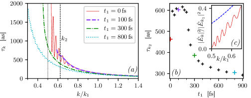
Figure 4: (a) Spectral relative group delay $\tau_{k}$ for the plastic target as a function of wavenumber $k$ of an XUV probe pulse with pump–probe delays $t_{1}=0$, $100$, $300$ and $800\rm\,fs$ between peak intensities of the two pulses. The vertical dotted line corresponds to the plasma frequency at the original target density. (b) Relative group delay $\tau_{k_{2}}$ at the wavenumber $k_{2}=0.625\,k_{1}$ (vertical dashed line in panel a) as a function of pump–probe delay $t_{1}$. Coloured markers correspond to the same-coloured curves plotted in panel (a). (c) Spectral intensity $|\hat{E}_{k}|^{2}/|\hat{E}_{k_{1}}|^{2}$ of the initial (dashed blue line) and transmitted (solid red line) probe pulse for the $t_{1}=0{\rm\,fs}$ case.

Figure 5(a) shows the corresponding relative group delays in the aluminium plasma. As with the plastic target the $\tau_{k}$ curves are only plotted in the wavenumber range where $|\hat{E}_{k}|^{2}/|\hat{E}_{k_{1}}|^{2}>0.05$. With the aluminium target, this cutoff moves down in $k$ much faster and farther than in fig. 4(a), which indicates that the maximum density of the thinner aluminium drops faster than in the plastic target. In addition . as in fig. 4(a), the $\tau_{k}$ curve oscillates for $t_{1}=0{\rm\,fs}$ due to the same type of thin-film interference. The energy spectrum, shown in fig. 5(c), has stronger, albeit fewer, interference fringes than with the plastic target.

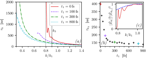
Figure 5: (a) Spectral relative group delay $\tau_{k}$ for the aluminium target as a function of wavenumber $k$ of an XUV probe pulse with pump–probe delays $t_{1}=0$, $100$, $300$ and $800\rm\,fs$ between peak intensities of the two pulses. The vertical dotted line corresponds to the plasma frequency at the original target density. (b) Relative group delay $\tau_{k_{3}}$ at the wavenumber $k_{3}=0.90\,k_{1}$ (vertical dashed line in panel a) as a function of pump–probe delay $t_{1}$. Coloured markers correspond to the same-coloured curves plotted in panel (a). (c) Spectral intensity $|\hat{E}_{k}|^{2}/|\hat{E}_{k_{1}}|^{2}$ of the initial (dashed blue line) and transmitted (solid red line) probe pulse for the $t_{1}=0{\rm\,fs}$ case.

Unlike with the plastic target, there is no initial compression of the electrons, which results in a monotonically decreasing $\tau_{k_{3}}$ in fig. 5(b), for $k_{3}=0.9k_{1}$. This observation is consistent with the direct findings from the PIC simulations shown in fig. 1(b) and 2(b): that the aluminium target lacks a defined compression wave, and that the inside expansion fronts propagating from both sides of the plasma meet more rapidly in the thinner target.

Another feature seen in fig. 5(b) is that $\tau_{k_{3}}$ has an initially steep decay which then changes slope quite abruptly in a knee at $t_{1}\simeq 150{\rm\,fs}$ (corresponding to a simulation time of $t\simeq 230{\rm\,fs}$, cf. fig. 2b). This is an interesting observation because the knee coincides with the meeting of the expansion fronts and broadening of the density peaks, which can be observed directly from the PIC simulation: see the $\tilde{\omega}_{\mathrm{p}}^{2}$ profiles at $t=150{\rm\,fs}$ and $230{\rm\,fs}$ in fig. 2(b). A similar, but less-pronounced, knee can also be seen with the dispersion in the plastic target for $t_{1}\simeq 250{\rm\,fs}$ (simulation time $t\simeq 330{\rm\,fs}$). The reason why the knee is less pronounced in the plastic target is probably that the thicker plastic target has a wider base density, so that the dispersion is less dominated by the narrow density peak.

Furthermore, the initial slope of the decay of $\tau_{k_{3}}$ is correlated with the rate of decrease of the peak density. This relationship can be understood via the group velocity of the plasma dispersion $v_{\rm gr}=c\,(1-\tilde{\omega}_{\mathrm{p}}^{2}/\omega^{2})^{1/2}$, which goes to zero if $\tilde{\omega}_{\mathrm{p}}$ reaches $\omega$; if we have a density peak close to the critical density, then the group delays $\tau_{k}\sim 1/v_{\rm gr}$ near the peak plasma frequency will be dominated by that peak. In the aluminium case shown in fig. 5(b), with $k_{3}$ quite close to the initial plasma frequency, $\tau_{k_{3}}$ is first dominated by the peak density, which is in the form of a narrow peak that decays rapidly. Later, when the plasma expansion also starts to flatten the density peak ($t=230{\rm\,fs}$ in fig. 2b), other contributions to the dispersion – such as the width of the plasma, which evolves more slowly – also become important. Note, however, that it is more difficult to infer the absolute value of the peak density, since the absolute value of the group delay will also be affected by the rest of the plasma – by a more slowly varying additive shift – as well as phase shifts when entering/exiting the plasma. However, it appears feasible to use XUV dispersion as a direct diagnostic to infer the evolution of the plasma experimentally.

In the high-wavenumber end of the spectrum, we find another remarkable feature of the $\tau_{k}$ curves in figs. 4(a) and 5(a): they all converge in the high-wavenumber limit. Furthermore, they converge toward the same values for both the plastic and aluminium targets, e.g. $\tau_{k}\approx 40{\rm\,as}$ at $k=1.8\,k_{1}$ (outside the ranges displayed in figs. 4a and 5a). This observation can again be understood by analysing the group velocity in the plasma. The group delay, after propagation a distance $\ell$, at a frequency $\omega^{\prime}$ can be approximated via a Wentzel–Kramers–Brillouin (WKB) approximation (for slowly varying spatial features and ignoring time variation) as

$$\tau(\omega^{\prime})+\frac{\ell}{c}\simeq\int_{0}^{\ell}\frac{\differential{x}}{v_{\rm gr}(x;\omega^{\prime})}=\int_{0}^{\ell}\frac{\differential{x}}{c\sqrt{1-\tilde{\omega}^{2}_{\mathrm{p}}(x)/{\omega^{\prime}}^{2}}}.$$ (14)

As the group delay, as defined in (13), does not take vacuum propagation into account, a term $\ell/c$ has to be added to the left-hand side in order to agree with the integral. Note that with the vacuum propagation accounted for separately in this way, the integration limits can be chosen arbitrarily large, as long as they are outside the plasma. Next, in the high-frequency limit, the square root can be expanded and we obtain

$$\tau(\omega^{\prime}\gg\tilde{\omega}^{2}_{\mathrm{p}})\approx\frac{1}{2c}\int_{0}^{\ell}\frac{\tilde{\omega}^{2}_{\mathrm{p}}(x)}{{\omega^{\prime}}^{2}}\differential{x}\simeq\frac{1}{2c}\,\quantity(\frac{\omega_{1}}{\omega^{\prime}})^{2}\!\int_{0}^{\ell}\frac{n_{\mathrm{e}}(x)}{n_{\rm c,1}}\differential{x};$$ (15)

we remind the reader that $\omega_{1}$ and $n_{\rm c,1}$ are the central frequency and associated critical density of the probe pulse, respectively. In the last step we also used the approximation $\tilde{\gamma}\simeq 1$, which holds for temperatures $T_{\mathrm{e}}\lesssim 10{\rm\,keV}$. The group delay at high frequencies is therefore a measure of the line-integrated density, which can be used to follow the transverse electron transport away from the optical axis during the plasma expansion.

The fact that all the curves in figs. 4(a) and 5(a) converge toward the same value in the high-wavenumber limit means that the line-integrated density of the two plasma on the optical axis, has not changed significantly during the course of the PIC simulation: recall that the initial line-integrated densities of the two targets were chosen to be approximately equal. We may also compare the observed $\tau_{k^{\prime}}\approx 40{\rm\,as}$ at $k^{\prime}=1.8\,k_{1}$ ($\omega^{\prime}=1.8\,\omega_{1}$) against the known line integrated densities from the PIC simulations. For the plastic target, the initial density profile is trapezoidal and can easily be integrated in (15) to give a WKB-approximated group delay of $39{\rm\,as}$. The remarkable agreement between the WKB and PS methods is a useful sanity check for the PS computation.

In the dispersion analysis of this paper, we have assumed the amplitude of the XUV probe pulse to be small, which allows for the linearised treatment of the wave evolution. Although theoretically convenient, in an experiment, the amplitude of the probe pulse must be significantly higher than the radiation generated – in the relevant spectral band – by the plasma itself, e.g. through bremsstrahlung (BS) and recombination. Regarding the emission due to recombination, it will be in a limited number of well-defined wavelengths, which will affect the dispersion measurements for those specific wavelengths. It should, however, still be possible to obtain a clean measurements of group delays for the other XUV wavelengths in the probe-pulse spectrum.

The BS, however, presents a broad-spectrum background noise to the measurement, thus the XUV probe should have a higher energy than the detected BS in order to reach a high signal-to-noise ratio. We estimate the emitted BS power, in the spectral range down to $5{\rm\,nm}$ wavelength, to be in the order of $10^{6}{-}10^{7}{\rm\,W}$ for the plasmas considered in this paper. However, the BS is emitted isotropically, whereas the probe pulse is highly directional. The focused XUV pulse reported by Coudert-Alteirac et al. (2017) had an angular divergence of less than approximately $1{\rm\,mrad}$, corresponding to a solid angle of $3\times 10^{-6}{\rm\,sr}$. Therefore, if the XUV detection is made with a comparable angular discrimination, the detected power from the BS would only be in the order of $3{-}30{\rm\,W}$. Recently, Morris, Robinson & Ridgers (2021) have shown significantly longer durations of BS emissions than previous literature, up to $10{-}100{\rm\,ps}$, however that is for much larger target volumes than considered here. Even with this very conservative estimate of the duration, the detected BS energy would only be in the $0.3{-}3{\rm\,nJ}$ range. In comparison, Manschwetus et al. (2016) reports an on-target XUV pulse energy of $40{\rm\,nJ}$, which is sufficiently greater than the (discriminated) BS power, making group-delay measurements with the RABBIT or attosecond streak camera methods feasible. In addition, the signal in these measurements is encoded as a temporal oscillation with the delay between the XUV pulses and the external infrared measurement pulse (employed in the RABBIT or streaking measurement mechanisms), which would further aid to discriminate the sought signal information from the BS background noise.

6 Conclusions

In this paper, we have presented a synthetic XUV dispersion diagnostic method, which can be used with the output of a PIC simulation. The use of XUV frequencies allow for probing of some solid-density plasmas, which are otherwise over-critical for optical wavelengths. The synthetic dispersion generated could then be used in comparisons with experiments, which would aid experimental validation efforts and the understanding of the evolution of the laser-generated plasma. The propagation of the XUV probe pulse is accurately calculated using a 1D PS solver along the optical axis. Then the group delays of the frequency components of the pulse are computed from the complex phases of the spectral components. As a part of the dispersion calculation, we present a linearised kinetic correction to the plasma frequency, relevant for plasmas that have a significant fraction of relativistic electrons. However, for experimentally relevant pump-pulse parameters, this correction only entails a decrease in effective plasma frequency in the order of a few per cent. The main quantity being probed is, therefore, the electron density profile. To some extent, both the maximum and the line-integrated value of the density can be inferred from the group delays in the XUV pulse caused by the dispersion.

We have illustrated this synthetic diagnostic technique on thin foil targets, where we show that the change in group delays of the XUV pulse varies significantly for different probe delay times. Indeed, the group delays reported here are well within currently available experimental resolution (López-Martens et al., 2005). Furthermore, this technique allows for an unprecedented time resolution of the plasma evolution, which is of great use in experimental validation of PIC simulations. This technique might also be used as a direct diagnostic for the evolution of the peak density in the plasma profile, as well as the line-integrated density. Furthermore, the presence of thin-film interference could be used to study the early evolution of the plasma surface.

Acknowledgements

The authors are grateful for fruitful discussions with E. Siminos, L. Gremillet, P. Tassin, C. Riconda, M. Hoppe, as well as F. Pérez for support with Smilei. J. Hellsvik at PDC Center for High Performance Computing is acknowledged for assistance in making Smilei run on the PDC resources.

Funding

This project has received funding from the Knut and Alice Wallenberg Foundation (Dnr. KAW 2020.0111). The computations were enabled by resources provided by the Swedish National Infrastructure for Computing (SNIC), partially funded by the Swedish Research Council through grant agreement no. 2018-05973.

Declaration of interests

The authors report no conflict of interest.

Appendix A Relativistic plasma frequency in thermal plasmas

For an isotropic distribution, i.e. $4\pi{}p^{2}f({\bf\it p})=f(p)$, we can write (7) as

$$\tilde{\gamma}^{-1}_{\hat{{\bf\it e}}}=\int\!\differential[3]{p}\frac{\bar{f}({\bf\it p})}{\gamma}\quantity(1-\frac{({\bf\it p}\dotproduct\hat{{\bf\it e}})^{2}}{\gamma^{2}})=\int\!\differential{p}\differential{\theta}\differential{\varphi}\,\sin\theta\,\frac{\bar{f}(p)}{4\pi\gamma}\quantity(1-\frac{p^{2}\cos^{2}\theta}{\gamma^{2}}),$$ (16)

where $\bar{f}=f/n_{\mathrm{e}}$ denote the density-normalised distribution such that $\int\differential[3]{p}\,\bar{f}({\bf\it p})=1$, and where we have aligned the $\theta=0$ axis along $\hat{{\bf\it e}}$ direction. Performing the angular integrals yields the effective gamma factor for an isotropic distribution as

$$\tilde{\gamma}^{-1}=\frac{1}{3}\int_{0}^{\infty}\!\differential{p}\frac{\bar{f}(p)}{\gamma}\quantity(2+\frac{1}{\gamma^{2}})=\frac{1}{3}\int_{1}^{\infty}\!\differential{\gamma}\frac{\bar{f}(\gamma)}{\gamma}\,\quantity(2+\frac{1}{\gamma^{2}}),$$ (17)

where in the last integral, we have changed variables to $\gamma=(1+p^{2})^{1/2}$, and we have absorbed the Jacobian into the distribution function, i.e. $\bar{f}(p)\differential{p}=\bar{f}(\gamma)\differential{\gamma}$. This expression for $\tilde{\gamma}^{-1}$ naturally does not have a polarisation dependence.

With (17), we can calculate $\tilde{\gamma}^{-1}$ from a thermal plasma, using the Maxwell–Jüttner distribution

$$\bar{f}_{\rm MJ}(\gamma)=\frac{\varTheta}{K_{2}(\varTheta)}\,\gamma\sqrt{\gamma^{2}-1}\mathrm{e}^{-\varTheta\gamma}.$$ (18)

where $\varTheta=m_{\mathrm{e}}c^{2}/T_{\mathrm{e}}$ is the dimensionless inverse electron temperature, and $K_{2}$ is the modified Bessel function of the second kind (of order two). If we take this distribution in (17), we obtain

$$\tilde{\gamma}^{-1}_{\rm MJ}={} \frac{\varTheta}{3K_{2}(\varTheta)}\int_{1}^{\infty}\differential{\gamma}\sqrt{\gamma^{2}-1}\mathrm{e}^{-\varTheta\gamma}\,\quantity(2+\frac{1}{\gamma^{2}})$$ (19a)

$$={} \frac{2K_{1}(\varTheta)}{3K_{2}(\varTheta)}+\frac{\varTheta}{3K_{2}(\varTheta)}\int_{1}^{\infty}\differential{\gamma}\frac{\sqrt{\gamma^{2}-1}}{\gamma^{2}}\mathrm{e}^{-\varTheta\gamma}.$$ (19b)

The last integral can be solved numerically, the result of which is shown in fig. 6.

In order to obtain an explicit analytic result, we can perform the same calculation for non-relativistic temperatures, $\varTheta\gg 1$. Using the Maxwell–Boltzmann distribution,

$$\bar{f}_{\rm MB}(p)=\frac{4\pi}{(2\pi/\varTheta)^{3/2}}\mathrm{e}^{-\varTheta\,p^{2}/2},$$ (20)

in (17) yields

$$\tilde{\gamma}^{-1}_{\rm MB}=\frac{\varTheta^{3/2}\mathrm{e}^{\varTheta/4}}{6\sqrt{2\pi}}\quantity[\varTheta K_{0}(\varTheta/4)+(2-\varTheta)K_{1}(\varTheta/4)].$$ (21)

By asymptotically expanding the Bessel functions in (21) for $\varTheta\to\infty$, we find the low-temperature asymptotic behaviour

$$1-\tilde{\gamma}^{-1}\simeq\frac{5}{2\varTheta}=\frac{5T_{\mathrm{e}}}{2m_{\mathrm{e}}c^{2}}\mbox{\quad as\quad}\varTheta\to\infty\quad(T_{\mathrm{e}}\to 0),$$ (22)

where we have expressed the asymptotic behaviour in terms of the relative reduction of the squared plasma frequency, $1-\tilde{\gamma}=1-\tilde{\omega}_{\mathrm{p}}^{2}/\omega_{\mathrm{p}}^{2}$. Naturally, (22) is also an asymptote to (19) as the Maxwell–Jüttner distribution approaches the Maxwell–Boltzmann distribution for low temperatures.

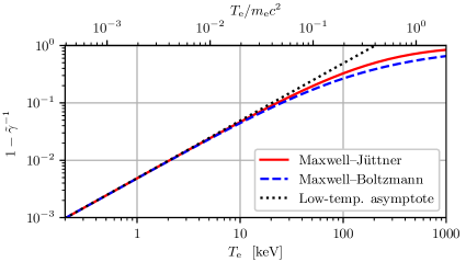
Figure 6: Relative reduction of the squared plasma frequency due to the effective gamma factor, $1-\tilde{\gamma}^{-1}$, for both Maxwell–Jüttner (solid red line) and Maxwell–Boltzmann (blue dashed line) distributed electrons with temperature $T_{\mathrm{e}}$. The curves for both distributions display an asymptotic behaviour $1-\tilde{\gamma}^{-1}\simeq 5T_{\mathrm{e}}/(2m_{\mathrm{e}}c^{2})$ as $T_{\mathrm{e}}\to 0$ (black dotted line).

As can be seen in fig. 6, when we numerically compare the relativistic (19) and the non-relativistic (21) effective gamma factors, we find that the two expressions agree well with each other (to within 5%) up to temperatures of $T_{\mathrm{e}}\sim 10{\rm\,keV}$. In either case, the relative reduction of the squared plasma frequency, $1-\tilde{\gamma}=1-\tilde{\omega}_{\mathrm{p}}^{2}/\omega_{\mathrm{p}}^{2}$, remains below 5% for temperatures less than $10{\rm\,keV}$. We also see that the low-temperature asymptote is a good approximation of the full solutions, up to temperatures of several kiloelectronvolts.

Appendix B Benchmarking of the PS solver

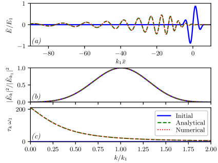
Figure 7: Benchmark test of the PS solver: propagation for $1{\rm\,\text{\textmu}{m}}$ through a homogeneous plasma with $\omega_{\mathrm{p}}=0.5\,\omega_{1}$. A comparison is shown of the initial (solid line), analytically (dashed line) and numerically propagated (dotted line) probe pulses. (a) Real-space waveforms of the corresponding pulses. The positional coordinate $\bar{x}$ is relative to the vacuum propagation position of the pulse centre. (b) Energy spectra of the corresponding pulses. (c) relative group delay $\tau_{k}$ of the numerically and analytically propagated pulses.

In order to evaluate the numerical accuracy of the PS solver, we have benchmarked it by propagating a test pulse through a homogeneous plasma. The analytical dispersion of a pulse in a homogeneous plasma with plasma frequency $\omega_{\mathrm{p}}$ is given by $\hat{E}_{k}(t)=\hat{E}_{k}(t{=}0)\,\exp(-\mathrm{i}\omega_{k}t),$ where $\omega_{k}={\rm sgn}(k)\,(c^{2}k^{2}+\omega_{\mathrm{p}}^{2})^{1/2}$ according to the plasma dispersion. Note that, unlike in the main body of the paper, the pulse is initialised with the waveform shown in fig. 7(a) already inside the plasma, which means that the wavenumber spectrum, shown in fig. 7(b), still goes all the way down to $k=0$ (corresponding to $\omega=\omega_{\mathrm{p}}$); this is unlike in the main body of the paper, where the pulse is initialised – and then later measured – in vacuum and, therefore, the transmitted part of the pulse gets cut off below $k_{\text{cutoff}}=\omega_{\mathrm{p}}/c$. The benchmark tests were performed with the same numerical settings as used in the main body of the paper, described in § 4.2.

Figure 7 shows the results from one such benchmark, where the pulse has been propagated for $1{\rm\,\text{\textmu}{m}}$ through a plasma with plasma frequency $\omega_{\mathrm{p}}=0.5\,\omega_{1}$ (i.e. $n_{\mathrm{e}}=0.25n_{\rm c}$), where $\omega_{1}$ is the central frequency of the test pulse. This plasma frequency is close to that of the plastic target used in this paper. Figure 7(a) shows the initial (solid blue line) pulse real-space waveform as well as the analytically (dashed green line) and numerically (dotted red line) propagated pulses. There is no discernible difference between the analytical and numerical cases. Figure 7(b) shows the energy spectrum, for the three cases as above, and fig. 7(c) shows the relative group delay $\tau_{k}=\rmDelta\bar{\phi}_{k}/\rmDelta\omega$ from § 3.1. Again, there is no discernible difference between the numerical and analytical curves; the relative error between the PS numerical and analytical dispersion, as represented by $\tau_{k}$, is less than $10^{-5}$ in the wavenumber range $0\leq{}k\leq 2\,k_{1}$. Similar performances are seen when the plasma density is varied between $\omega_{\mathrm{p}}=0$ (vacuum) and $\omega_{\mathrm{p}}=0.8\,\omega_{1}$ (aluminium), and with varying propagation lengths up to $10{\rm\,\text{\textmu}{m}}$. These benchmark tests demonstrate the extremely low numerical dispersion of the PS solver.

References

- Arefiev et al. (2020) Arefiev, A., Stark, D. J., Toncian, T. & Murakami, M. 2020 “Birefringence in thermally anisotropic relativistic plasmas and its impact on laser–plasma interactions”. Physics of Plasmas 27 (6), 063 106, doi: 10.1063/5.0008018
- Brown et al. (2011) Brown, C. R. D., Hoarty, D. J., James, S. F., Swatton, D., Hughes, S. J., Morton, J. W., Guymer, T. M., Hill, M. P., Chapman, D. A., Andrew, J. E., Comley, A. J., Shepherd, R., Dunn, J., Chen, H., Schneider, M., Brown, G., Beiersdorfer, P. & Emig, J. 2011 “Measurements of electron transport in foils irradiated with a picosecond time scale laser pulse”. Phys. Rev. Lett. 106, 185 003, doi: 10.1103/PhysRevLett.106.185003
- Calegari et al. (2016) Calegari, F., Sansone, G., Stagira, S., Vozzi, C. & Nisoli, M. 2016 “Advances in attosecond science”. Journal of Physics B: Atomic, Molecular and Optical Physics 49 (6), 062 001, doi: 10.1088/0953-4075/49/6/062001
- Chen et al. (2009) Chen, S. N., Patel, P. K., Chung, H.-K., Kemp, A. J., Le Pape, S., Maddox, B. R., Wilks, S. C., Stephens, R. B. & Beg, F. N. 2009 “X-ray spectroscopy of buried layer foils irradiated at laser intensities in excess of 1020 W/cm2”. Phys. Plasmas 16 (6), 062 701, doi: 10.1063/1.3143715
- Coudert-Alteirac et al. (2017) Coudert-Alteirac, H., Dacasa, H., Campi, F., Kueny, E., Farkas, B., Brunner, F., Maclot, S., Manschwetus, B., Wikmark, H., Lahl, J., Rading, L., Peschel, J., Major, B., Varjú, K., Dovillaire, G., Zeitoun, P., Johnsson, P., L’Huillier, A. & Rudawski, P. 2017 “Micro-focusing of broadband high-order harmonic radiation by a double toroidal mirror”. Applied Sciences 7 (11), 1159, doi: 10.3390/app7111159
- Derouillat et al. (2018) Derouillat, J., Beck, A., Pérez, F., Vinci, T., Chiaramello, M., Grassi, A., Flé, M., Bouchard, G., Plotnikov, I., Aunai, N., Dargent, J., Riconda, C. & Grech, M. 2018 “Smilei: A collaborative, open-source, multi-purpose particle-in-cell code for plasma simulation”. Comput. Phys. Commun. 222, 351, doi: 10.1016/j.cpc.2017.09.024
- Descamps et al. (2000) Descamps, D., Lyngå, C., Norin, J., L’Huillier, A., Wahlström, C.-G., Hergott, J.-F., Merdji, H., Salières, P., Bellini, M. & Hänsch, T. 2000 “Extreme ultraviolet interferometry measurements with high-order harmonics”. Optics letters 25 (2), 135–137, doi: 10.1364/OL.25.000135
- Dobosz et al. (2005) Dobosz, S., Doumy, G., Stabile, H., D’Oliveira, P., Monot, P., Réau, F., Hüller, S. & Martin, P. 2005 “Probing hot and dense laser-induced plasmas with ultrafast xuv pulses”. Phys. Rev. Lett. 95, 025 001, doi: 10.1103/PhysRevLett.95.025001
- Drake (2018) Drake, R. P. 2018 “A journey through high-energy-density physics”. Nuclear Fusion 59 (3), 035 001, doi: 10.1088/1741-4326/aaf0e3
- Ferray et al. (1988) Ferray, M., L’Huillier, A., Li, X. F., Lompre, L. A., Mainfray, G. & Manus, C. 1988 “Multiple-harmonic conversion of 1064 nm radiation in rare gases”. Journal of Physics B: Atomic, Molecular and Optical Physics 21 (3), L31–L35, doi: 10.1088/0953-4075/21/3/001
- Godfrey (1974) Godfrey, B. B. 1974 “Numerical Cherenkov instabilities in electromagnetic particle codes”. Journal of Computational Physics 15 (4), 504–521, doi: 10.1016/0021-9991(74)90076-X
- Hergott et al. (2001) Hergott, J.-F., Salières, P., Merdji, H., le Déroff, L., Carré, B., Auguste, T., Monot, P., d’Oliveira, P., Descamps, D., Norin, J., Lyngå, C., L’Huillier, A., Wahlström, C.-G., Bellini, M. & Huller, S. 2001 “XUV interferometry using high-order harmonics: Application to plasma diagnostics”. Laser and Particle Beams 19 (1), 35–40, doi: 10.1017/S0263034601191056
- Hergott et al. (2003) Hergott, J.-F., Auguste, T., Salières, P., Le Déroff, L., Monot, P., d’Oliveira, P., Campo, D., Merdji, H. & Carré, B. 2003 “Application of frequency-domain interferometry in the extreme-ultraviolet range by use of high-order harmonics”. JOSA B 20 (1), 171–181, doi: 10.1364/JOSAB.20.000171
- Higginson et al. (2018) Higginson, A., Gray, R. J., King, M., Dance, R. J., Williamson, S. D. R., Butler, N. M. H., Wilson, R., Capdessus, R., Armstrong, C., Green, J. S., Hawkes, J., Martin, P., Wei, W. Q., Mirfayzi, S. R., Yuan, X. H., Kar, S., Borghesi, M., Clarke, R. J., Neely, D. & McKenna, P. 2018 “Near-100 MeV protons via a laser-driven transparency-enhanced hybrid acceleration scheme”. Nat. Commun. 9 (1), 724, doi: 10.1038/s41467-018-03063-9
- Itatani et al. (2002) Itatani, J., Quéré, F., Yudin, G. L., Ivanov, M. Y., Krausz, F. & Corkum, P. B. 2002 “Attosecond streak camera”. Phys. Rev. Lett. 88, 173 903, doi: 10.1103/PhysRevLett.88.173903
- Jones et al. (2001–) Jones, E., Oliphant, T., Peterson, P. et al. 2001– “SciPy: Open source scientific tools for Python”. URL http://www.scipy.org/
- Juno et al. (2020) Juno, J., Swisdak, M. M., Tenbarge, J. M., Skoutnev, V. & Hakim, A. 2020 “Noise-induced magnetic field saturation in kinetic simulations”. Journal of Plasma Physics 86 (4), 175860 401, doi: 10.1017/S0022377820000707
- Kaw & Dawson (1970) Kaw, P. & Dawson, J. 1970 “Relativistic nonlinear propagation of laser beams in cold overdense plasmas”. The Physics of Fluids 13 (2), 472–481, doi: 10.1063/1.1692942
- Kluge et al. (2018) Kluge, T., Rödel, M., Metzkes-Ng, J., Pelka, A., Garcia, A. L., Prencipe, I., Rehwald, M., Nakatsutsumi, M., McBride, E. E., Schönherr, T., Garten, M., Hartley, N. J., Zacharias, M., Grenzer, J., Erbe, A., Georgiev, Y. M., Galtier, E., Nam, I., Lee, H. J., Glenzer, S., Bussmann, M., Gutt, C., Zeil, K., Rödel, C., Hübner, U., Schramm, U. & Cowan, T. E. 2018 “Observation of ultrafast solid-density plasma dynamics using femtosecond x-ray pulses from a free-electron laser”. Phys. Rev. X 8, 031 068, doi: 10.1103/PhysRevX.8.031068
- Koliyadu et al. (2017) Koliyadu, J. C. P., Künzel, S., Wodzinski, T., Keitel, B., Duarte, J., Williams, G. O., João, C. P., Pires, H., Hariton, V., Galletti, M., Gomes, N., Figueira, G., Dias, J. M., Lopes, N., Zeitoun, P., Plönjes, E. & Fajardo, M. 2017 “Optimization and characterization of high-harmonic generation for probing solid density plasmas”. Photonics 4 (2), 25, doi: 10.3390/photonics4020025
- Le Pape et al. (2018) Le Pape, S., Berzak Hopkins, L. F., Divol, L., Pak, A., Dewald, E. L., Bhandarkar, S., Bennedetti, L. R., Bunn, T., Biener, J., Crippen, J., Casey, D., Edgell, D., Fittinghoff, D. N., Gatu-Johnson, M., Goyon, C., Haan, S., Hatarik, R., Havre, M., Ho, D. D.-M., Izumi, N., Jaquez, J., Khan, S. F., Kyrala, G. A., Ma, T., Mackinnon, A. J., MacPhee, A. G., MacGowan, B. J., Meezan, N. B., Milovich, J., Millot, M., Michel, P., Nagel, S. R., Nikroo, A., Patel, P., Ralph, J., Ross, J. S., Rice, N. G., Strozzi, D., Stadermann, M., Volegov, P., Yeamans, C., Weber, C., Wild, C., Callahan, D. & Hurricane, O. A. 2018 “Fusion energy output greater than the kinetic energy of an imploding shell at the national ignition facility”. Phys. Rev. Lett. 120, 245 003, doi: 10.1103/PhysRevLett.120.245003
- López-Martens et al. (2005) López-Martens, R., Varjú, K., Johnsson, P., Mauritsson, J., Mairesse, Y., Salières, P., Gaarde, M. B., Schafer, K. J., Persson, A., Svanberg, S., Wahlström, C.-G. & L’Huillier, A. 2005 “Amplitude and phase control of attosecond light pulses”. Phys. Rev. Lett. 94, 033 001, doi: 10.1103/PhysRevLett.94.033001
- Major et al. (2021) Major, B., Ghafur, O., Kovács, K., Varjú, K., Tosa, V., Vrakking, M. J. J. & Schütte, B. 2021 “Compact intense extreme-ultraviolet source”. Optica 8 (7), 960–965, doi: 10.1364/OPTICA.421564
- Manschwetus et al. (2016) Manschwetus, B., Rading, L., Campi, F., Maclot, S., Coudert-Alteirac, H., Lahl, J., Wikmark, H., Rudawski, P., Heyl, C. M., Farkas, B., Mohamed, T., L’Huillier, A. & Johnsson, P. 2016 “Two-photon double ionization of neon using an intense attosecond pulse train”. Phys. Rev. A 93, 061 402, doi: 10.1103/PhysRevA.93.061402
- Merdji et al. (2000) Merdji, H., Salières, P., le Déroff, L., Hergott, J.-F., Carré, B., Joyeux, D., Descamps, D., Norin, J., Lyngå, C., L’Huillier, A., Wahlström, C.-G., Bellini, M. & Huller, S. 2000 “Coherence properties of high-order harmonics: Application to high-density laser–plasma diagnostic”. Laser and Particle Beams 18 (3), 495–502, doi: 10.1017/S026303460018320X
- Morris, Robinson & Ridgers (2021) Morris, S., Robinson, A. & Ridgers, C. 2021 “Highly efficient conversion of laser energy to hard x-rays in high-intensity laser–solid simulations”. Physics of Plasmas 28 (10), 103 304, doi: 10.1063/5.0055398
- Neely et al. (2006) Neely, D., Foster, P., Robinson, A., Lindau, F., Lundh, O., Persson, A., Wahlström, C.-G. & McKenna, P. 2006 “Enhanced proton beams from ultrathin targets driven by high contrast laser pulses”. Applied Physics Letters 89 (2), 021 502, doi: 10.1063/1.2220011
- Nürnberg et al. (2009) Nürnberg, F., Schollmeier, M., Brambrink, E., Blažević, A., Carroll, D. C., Flippo, K., Gautier, D. C., GeiSSel, M., Harres, K., Hegelich, B. M., Lundh, O., Markey, K., McKenna, P., Neely, D., Schreiber, J. & Roth, M. 2009 “Radiochromic film imaging spectroscopy of laser-accelerated proton beams”. Review of Scientific Instruments 80 (3), 033 301, doi: 10.1063/1.3086424
- Nuter et al. (2014) Nuter, R., Grech, M., de Alaiza Martinez, P. G., Bonnaud, G. & d’Humieres, E. 2014 “Maxwell solvers for the simulations of the laser-matter interaction”. The European Physical Journal D 68 (6), 1–9, doi: 10.1140/epjd/e2014-50162-y
- Paul et al. (2001) Paul, P. M., Toma, E. S., Breger, P., Mullot, G., Augé, F., Balcou, Ph., Muller, H. G. & Agostini, P. 2001 “Observation of a train of attosecond pulses from high harmonic generation”. Science 292 (5522), 1689–1692, doi: 10.1126/science.1059413
- Pérez et al. (2010) Pérez, F., Gremillet, L., Koenig, M., Baton, S. D., Audebert, P., Chahid, M., Rousseaux, C., Drouin, M., Lefebvre, E., Vinci, T., Rassuchine, J., Cowan, T., Gaillard, S. A., Flippo, K. A. & Shepherd, R. 2010 “Enhanced isochoric heating from fast electrons produced by high-contrast, relativistic-intensity laser pulses”. Phys. Rev. Lett. 104, 085 001, doi: 10.1103/PhysRevLett.104.085001
- Pérez et al. (2012) Pérez, F., Gremillet, L., Decoster, A., Drouin, M. & Lefebvre, E. 2012 “Improved modeling of relativistic collisions and collisional ionization in particle-in-cell codes”. Phys. of Plasmas 19, 083 104, doi: 10.1063/1.4742167
- Remington et al. (1999) Remington, B. A., Arnett, D., Paul, R., Takabe, H. et al. 1999 “Modeling astrophysical phenomena in the laboratory with intense lasers”. Science 284 (5419), 1488–1493, doi: 10.1126/science.284.5419.1488
- Renaudin et al. (2003) Renaudin, P., Blancard, C., Clérouin, J., Faussurier, G., Noiret, P. & Recoules, V. 2003 “Aluminum equation-of-state data in the warm dense matter regime”. Phys. Rev. Lett. 91, 075 002, doi: 10.1103/PhysRevLett.91.075002
- Renner & Rosmej (2019) Renner, O. & Rosmej, F. B. 2019 “Challenges of x-ray spectroscopy in investigations of matter under extreme conditions”. Matter and Radiation at Extremes 4 (2), 024 201, doi: 10.1063/1.5086344
- Romagnani et al. (2005) Romagnani, L., Fuchs, J., Borghesi, M., Antici, P., Audebert, P., Ceccherini, F., Cowan, T., Grismayer, T., Kar, S., Macchi, A., Mora, P., Pretzler, G., Schiavi, A., Toncian, T. & Willi, O. 2005 “Dynamics of electric fields driving the laser acceleration of multi-MeV protons”. Phys. Rev. Lett. 95, 195 001, doi: 10.1103/PhysRevLett.95.195001
- Salières et al. (1999) Salières, P., Le Déroff, L., Auguste, T., Monot, P., d’Oliveira, P., Campo, D., Hergott, J.-F., Merdji, H. & Carré, B. 1999 “Frequency-domain interferometry in the XUV with high-order harmonics”. Phys. Rev. Lett. 83, 5483–5486, doi: 10.1103/PhysRevLett.83.5483
- Sävert et al. (2015) Sävert, A., Mangles, S. P. D., Schnell, M., Siminos, E., Cole, J. M., Leier, M., Reuter, M., Schwab, M. B., Möller, M., Poder, K., Jäckel, O., Paulus, G. G., Spielmann, C., Skupin, S., Najmudin, Z. & Kaluza, M. C. 2015 “Direct observation of the injection dynamics of a laser wakefield accelerator using few-femtosecond shadowgraphy”. Phys. Rev. Lett. 115, 055 002, doi: 10.1103/PhysRevLett.115.055002
- Schwab et al. (2020) Schwab, M. B., Siminos, E., Heinemann, T., Ullmann, D., Karbstein, F., Kuschel, S., Sävert, A., Yeung, M., Hollatz, D., Seidel, A., Cole, J., Mangles, S. P. D., Hidding, B., Zepf, M., Skupin, S. & Kaluza, M. C. 2020 “Visualization of relativistic laser pulses in underdense plasma”. Phys. Rev. Accel. Beams 23, 032 801, doi: 10.1103/PhysRevAccelBeams.23.032801
- Siminos et al. (2012) Siminos, E., Grech, M., Skupin, S., Schlegel, T. & Tikhonchuk, V. T. 2012 “Effect of electron heating on self-induced transparency in relativistic-intensity laser-plasma interactions”. Phys. Rev. E 86, 056 404, doi: 10.1103/PhysRevE.86.056404
- Siminos et al. (2014) Siminos, E., Sánchez-Arriaga, G., Saxena, V. & Kourakis, I. 2014 “Modeling relativistic soliton interactions in overdense plasmas: A perturbed nonlinear Schrödinger equation framework”. Phys. Rev. E 90, 063 104, doi: 10.1103/PhysRevE.90.063104
- Siminos et al. (2016) Siminos, E., Skupin, S., Sävert, A., Cole, J. M., Mangles, S. P. D. & Kaluza, M. C. 2016 “Modeling ultrafast shadowgraphy in laser-plasma interaction experiments”. Plasma Physics and Controlled Fusion 58 (6), 065 004, doi: 10.1088/0741-3335/58/6/065004
- Stark et al. (2015) Stark, D. J., Bhattacharjee, C., Arefiev, A. V., Toncian, T., Hazeltine, R. D. & Mahajan, S. M. 2015 “Relativistic plasma polarizer: Impact of temperature anisotropy on relativistic transparency”. Phys. Rev. Lett. 115, 025 002, doi: 10.1103/PhysRevLett.115.025002
- Starrett (2018) Starrett, C. E. 2018 “Coulomb log for conductivity of dense plasmas”. Physics of Plasmas 25 (9), 092 707, doi: 10.1063/1.5053124
- Sundström et al. (2020a) Sundström, A., Gremillet, L., Siminos, E. & Pusztai, I. 2020a “Fast collisional electron heating and relaxation with circularly polarized ultraintense short-pulse laser”. Journal of Plasma Physics 86 (2), 755860 201, doi: 10.1017/S0022377820000264
- Sundström et al. (2020b) Sundström, A., Gremillet, L., Siminos, E. & Pusztai, I. 2020b “Collisional effects on the ion dynamics in thin-foil targets driven by an ultraintense short pulse laser”. Plasma Physics and Controlled Fusion 62 (8), 085 015, doi: 10.1088/1361-6587/ab9a62
- Williams et al. (2013) Williams, G. O., Chung, H.-K., Vinko, S. M., Künzel, S., Sardinha, A. B., Zeitoun, Ph. & Fajardo, M. 2013 “Method of time resolved refractive index measurements of x-ray laser heated solids”. Physics of Plasmas 20 (4), 042 701, doi: 10.1063/1.4794964
- Zhang et al. (2017) Zhang, H., Shen, B. F., Wang, W. P., Zhai, S. H., Li, S. S., Lu, X. M., Li, J. F., Xu, R. J., Wang, X. L., Liang, X. Y., Leng, Y. X., Li, R. X. & Xu, Z. Z. 2017 “Collisionless shock acceleration of high-flux quasimonoenergetic proton beams driven by circularly polarized laser pulses”. Phys. Rev. Lett. 119, 164 801, doi: 10.1103/PhysRevLett.119.164801