Intent Contrastive Learning for Sequential Recommendation

Abstract.

Users’ interactions with items are driven by various intents (e.g., preparing for holiday gifts, shopping for fishing equipment, etc.). However, users’ underlying intents are often unobserved/latent, making it challenging to leverage such latent intents for Sequential recommendation (SR). To investigate the benefits of latent intents and leverage them effectively for recommendation, we propose Intent Contrastive Learning (ICL), a general learning paradigm that leverages a latent intent variable into SR. The core idea is to learn users’ intent distribution functions from unlabeled user behavior sequences and optimize SR models with contrastive self-supervised learning (SSL) by considering the learnt intents to improve recommendation. Specifically, we introduce a latent variable to represent users’ intents and learn the distribution function of the latent variable via clustering. We propose to leverage the learnt intents into SR models via contrastive SSL, which maximizes the agreement between a view of sequence and its corresponding intent. The training is alternated between intent representation learning and the SR model optimization steps within the generalized expectation-maximization (EM) framework. Fusing user intent information into SR also improves model robustness. Experiments conducted on four real-world datasets demonstrate the superiority of the proposed learning paradigm, which improves performance, and robustness against data sparsity and noisy interaction issues .

1. Introduction

Recommender systems have been widely used in many scenarios to provide personalized items to users over massive vocabularies of items. The core of an effective recommender system is to accurately predict users’ interests toward items based on their historical interactions. With the success of deep learning, deep Sequential Recommendation (SR) (Kang and McAuley, 2018; Sun et al., 2019) models, which aims at dynamically characterizing the behaviors of users with different deep neural networks (Yan et al., 2019; Wu et al., 2017), arguably represents the current state-of-the-art (Kang and McAuley, 2018; Sun et al., 2019; Ma et al., 2020; Zhou et al., 2020; Xie et al., 2020; Li et al., 2020a; Fan et al., 2021).

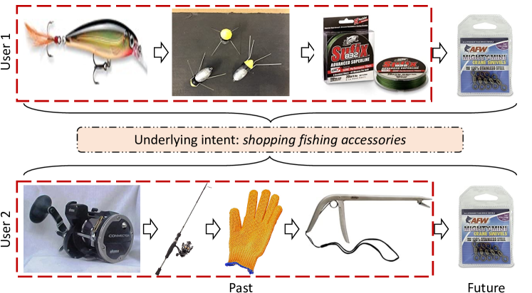
Figure 1. Users’ purchasing behaviors can be driven by underlying intents that are not observed.

In general, a deep SR model is trained based on users’ interaction behaviors via a deep neural network, assuming users’ interests depending on historical behaviors. However, consuming behaviour of users can be affected by other latent factors, i.e., driven by their underlying intents. Consider the example illustrated in Figure 1. Two users purchased a series of different items on Amazon in the past. Given such distinct interaction behaviors, the system will recommend different items to them. However, both of them are fishing enthusiasts and are shopping for fishing activities. As a result, they both purchase ‘fishing swivels’ in the future. If the system is aware that these two users are shopping for fishing activities, then commonly purchased items for fishing, such as ‘fishing swivels’ can be suggested. This motivates us to mine underlying intents that are shared across users and use the learnt intents to guide system providing recommendations.

Precisely discovering the intents of users, however, is under-explored. Most existing works (Tanjim et al., 2020; Cai et al., 2021) of user intent modeling require side information. ASLI (Tanjim et al., 2020) leverages user action types (e.g., click, add-to-favorite, etc.) to capture users’ intentions, whereas such information is not always available in system. CoCoRec (Cai et al., 2021) utilizes item category information. But we argue that categorical feature is unable to accurately represents users’ intents. For example, intents like ‘shopping for holiday gifts’ may involve items from multiple different categories. DSSRec (Ma et al., 2020) proposes a seq2seq training strategy, which optimizes the intents in latent spaces. However, those intents in DSSRec are inferred solely based on individual sequence representation, while ignoring the underlying correlations of the intents from different users.

Effectively modeling latent intents from user behaviors poses two challenges. First, it is extremely difficult to learn latent intents accurately because we have no labelling data for intents. The only available supervision signals for intents are the user behavior data. Nevertheless, as aforementioned example indicates, distinct behaviors may reflect the same intent. Besides, effectively fusing intent information into a SR model is non-trivial. The target in SR is to predict next items in sequences, which is solved by encoding sequences. Leveraging latent intents of sequences into the model requires the intent factors to be orthogonal to the sequence embeddings, which otherwise would induce redundant information.

To discover the benefits of latent intents and address challenges, we propose the Intent Contrastive Learning (ICL), a general learning paradigm that leverages the latent intent factor into SR. It learns users’ intent distributions from all user behavior sequences via clustering. And it leverages the learnt intents into the SR model via a new contrastive SSL, which maximizes the agreement between a view of sequence and its corresponding intent. The intent representation learning module and the contrastive SSL module are mutually reinforced to train a more expressive sequence encoder. We tackle the challenge of intent mining problem by introducing a latent variable to represent users’ intents and learn them alternately along with the SR model optimization through an expectation-maximization (EM) framework to ensure convergence. We suggest fusing learnt intent information into SR via the proposed contrastive SSL, as it can improve model’s performance as well as robustness. Extensive experiments conducted on four real-world datasets further verify the effectiveness of the proposed learning paradigm, which improves performance and robustness, even when recommender systems face heavy data sparsity issues.

2. Related Work

2.1. Sequential Recommendation

Sequential recommendation aims to accurately characterize users’ dynamic interests by modeling their past behavior sequences (Rendle, 2010; Rendle et al., 2010; Kang and McAuley, 2018; Chen et al., 2021; Li et al., 2021a; Liu et al., 2021a). Early works on SR usually model an item-to-item transaction pattern based on Markov Chains (Rendle, 2010; He and McAuley, 2016). FPMC (Rendle et al., 2010) combines the advantages of Markov Chains and matrix factorization to fuse both sequential patterns and users’ general interest. With the recent advances of deep learning, many deep sequential recommendation models are also developed (Tang and Wang, 2018; Hidasi et al., 2015; Kang and McAuley, 2018; Sun et al., 2019). Such as Convolutional Neural Networks (CNN)-based (Tang and Wang, 2018) and RNN-based (Hidasi et al., 2015) models. The recent success of Transformer (Vaswani et al., 2017) also motivates the developments of pure Transformer-based SR models. SASRec (Kang and McAuley, 2018) utilizes unidirectional Transformer to assign weights to each interacted item adaptively. BERT4Rec (Sun et al., 2019) improves that by utilizing a bidirectional Transformer with a Cloze task (Taylor, 1953) to fuse user behaviors information from left and right directions into each item. LSAN (Li et al., 2021a) improves SASRec on reducing model size perspective. It proposes a temporal context-aware embedding and twin-attention network, which are light weighted. ASReP (Liu et al., 2021b) further alleviates the data-sparsity issue by leveraging a pre-trained Transformer on the revised user behavior sequences to augment short sequences. In this paper, we study the potential of addressing data sparsity issues and improving SR via self-supervised learning.

2.2. User Intent for Recommendation

Recently, many approaches have been proposed to study users’ intents for improving recommendations (Wang et al., 2019b; Cen et al., 2020; Li et al., 2019; Li et al., 2021b). MCPRN (Wang et al., 2019b) designs mixture-channel purpose routing networks to adaptively learn users’ different purchase purposes of each item under different channels (sub-sequences) for session-based recommendation. MITGNN(Liu et al., 2020a) proposes a multi-intent translation graph neural network to mine users’ multiple intents by considering the correlations of the intents. ICM-SR (Pan et al., 2020) designs an intent-guided neighbor detector to retrieve correct neighbor sessions for neighbor representation. Different from session-based recommendation, another line of works focus on modeling the sequential dynamics of users’ interaction behaviors in a longer time span. DSSRec (Ma et al., 2020) proposes a seq2seq training strategy using multiple future interactions as supervision and introducing an intent variable from her historical and future behavior sequences. The intent variable is used to capture mutual information between an individual user’s historical and future behavior sequences. Two users of similar intents might be far away in representation space. Unlike this work, our intent variable is learned over all users’ sequences and is used to maximize mutual information across different users with similar learned intents. ASLI (Tanjim et al., 2020) captures intent via a temporal convolutional network with side information (e.g., user action types such as click, add-to-favorite, etc.), and then use the learned intents to guide SR model to predict the next item. Instead, our method can learn users’ intents based on user interaction data only.

2.3. Contrastive Self-Supervised Learning

Contrastive Self-Supervised Learning (SSL) has brought much attentions by different research communities including CV (Chen et al., 2020; Li et al., 2020b; He et al., 2020b; Caron et al., 2020; Khosla et al., 2020) and NLP (Gao et al., 2021; Gunel et al., 2020; Mnih and Kavukcuoglu, 2013; Zhang et al., 2020), as well as recommendation (Yao et al., 2020; Zhou et al., 2020; Wu et al., 2021; Xie et al., 2020). The fundamental goal of contrastive SSL is to maximize mutual information among the positive transformations of the data itself while improving discrimination ability to the negatives. In reccommendation, A two-tower DNN-based contrastive SSL model is proposed in (Yao et al., 2020). It aims to improving collaborative filtering based recommendation leveraging item attributes. SGL (Wu et al., 2021) adopts a multi-task framework with contrastive SSL to improve the graph neural networks (GCN)-based collaborative filtering methods (He et al., 2020a; Wang et al., 2019a; Liu et al., 2020b; Zhang and McAuley, 2020) with only item IDs as features. Specific to SR, S${}^{3}\text{-Rec}$ (Zhou et al., 2020) adopts a pre-training and fine-tuning strategy, and utilizes contrastive SSL during pre-training to incorporate correlations among items, sub-sequences, and attributes of a given user behavior sequence. However, the two-stage training strategy prevents the information sharing between next-item prediction and SSL tasks and restricts the performance improvement. CL4SRec (Xie et al., 2020) and CoSeRec (Liu et al., 2021a) instead utilize a multi-task training framework with a contrastive objective to enhance user representations. Different from them, our work is aware of users’ latent intent factor when leveraging contrastive SSL, which we show to be beneficial for improving recommendation performance and robustness.

3. Preliminaries

3.1. Problem definition

Assume that a recommender system has a set of users and items denoted by $\mathcal{U}$ and $\mathcal{V}$ respectively. Each user $u\in\mathcal{U}$ has a sequence of interacted items sorted in chronological order $S^{u}=[s^{u}_{1},\dots,s^{u}_{t},\dots,s^{u}_{|S^{u}|}]$ where $|S^{u}|$ is the number of interacted items and $s^{u}_{t}$ is the item $u$ interacted at step $t$. We denote $\mathbf{S}^{u}$ as embedded representation of $S^{u}$, where $\mathbf{s}^{u}_{t}$ is the d-dimensional embedding of item $s^{u}_{t}$. In practice, sequences are truncated with maximum length $T$. If the sequence length is greater than $T$, the most recent $T$ actions are considered. If the sequence length is less than $T$, ‘padding’ items will be added to the left until the length is $T$ (Tang and Wang, 2018; Hidasi et al., 2015; Kang and McAuley, 2018). For each user $u$, the goal of next item prediction task is to predict the next item that the user $u$ is most likely to interact with at the $|S_{u}|+1$ step among the item set $\mathcal{V}$, given sequence $\mathbf{S}^{u}$.  

3.2. Deep SR Models for Next Item Prediction

Modern sequential recommendation models commonly encode user behavior sequences with a deep neural network to model sequential patterns from (truncated) user historical behavior sequences. Without losing generality, we define a sequence encoder $f_{\theta}(\cdot)$ that encodes a sequence $\mathbf{S}^{u}$ and outputs user interest representations over all position steps $\mathbf{H}^{u}=f_{\theta}(\mathbf{S}^{u})$. Specially, $\mathbf{h}^{u}_{t}$ represents user’s interest at position $t$. The goal can be formulated as finding the optimal encoder parameter $\theta$ that maximizes the log-likelihood function of the expected next items of given $N$ sequences on all positional steps:

(1) $$\theta^{*}=\underset{\theta}{\mathrm{arg\,max}}~{}\sum_{u=1}^{N}\sum_{t=2}^{T}\ln P_{\theta}(s^{u}_{t}).$$

which is equivalent to minimizing the adapted binary cross-entropy loss as follows:

(2) $$\mathcal{L}_{\mathrm{NextItem}}=\sum_{u=1}^{N}\sum_{t=2}^{T}\mathcal{L}_{\mathrm{NextItem}}(u,t),$$

(3) $$\mathcal{L}_{\mathrm{NextItem}}(u,t)=-\log(\sigma(\mathbf{h}^{u}_{t-1}\cdot\mathbf{s}^{u}_{t}))-\sum_{neg}\log(1-\sigma(\mathbf{h}^{u}_{t-1}\cdot\mathbf{s}^{u}_{neg})),$$

where $\mathbf{s}^{u}_{t}$ and $\mathbf{s}^{u}_{neg}$ denote the embeddings of the target item $s_{t}$ and all items not interacted by $u$. The sum operator in Eq. 3 is computationally expensive because $|V|$ is large. Thus we follow (Kang and McAuley, 2018; Zhou et al., 2020; Cen et al., 2020) to use a sampled softmax technique to randomly sample a negative item for each time step in each sequence. $\sigma$ is the sigmoid function. And $N$ is refers to the mini-batch size as the SR model.

3.3. Contrastive SSL in SR

Figure 2. Overview of ICL. (a) An individual sequence level SSL for SR. (b) The proposed ICL for SR. It alternately performs intent representation learning and intent contrastive SSL with FNM within the generalized EM framework to maximizes mutual information (MIM) between a behavior sequence and its corresponding intent prototype.

Recent advances in contrastive SSL have inspired the recommendation community to leverage contrastive SSL to fuse correlations among different views of one sequence (Chen et al., 2020; Yao et al., 2020; Wu et al., 2021), following the mutual information maximization (MIM) principle. Existing approaches in SR can be seen as instance discrimination tasks that optimize a lower bound of MIM, such as InfoNCE (Oord et al., 2018; He et al., 2020b; Chen et al., 2020; Li et al., 2020b). It aims to optimize the proportion of gap of positive pairs and negative pairs (Liu et al., 2021c). In such an instance discrimination task, sequence augmentations such as ‘mask’, ‘crop’, or ‘reorder’ are required to create different views of the unlabeled data in SR (Sun et al., 2019; Zhou et al., 2020; Xie et al., 2020; Zhou et al., 2021). Formally, given a sequence $S^{u}$, and a pre-defined data transformation function set $\mathcal{G}$, we can create two positive views of $S^{u}$ as follows:

(4) $$\tilde{S}^{u}_{1}=g_{1}^{u}(S^{u}),\tilde{S}^{u}_{2}=g_{2}^{u}(S^{u}),\text{ s.t. }g_{1}^{u},g_{2}^{u}\sim\mathcal{G},$$

where $g_{1}^{u}$ and $g_{2}^{u}$ are transformation functions sampled from $\mathcal{G}$ to create a different view of sequence $s_{u}$. Commonly, views created from the same sequence are treated as positive pairs, and the views of any different sequences are considered as negative pairs. The augmented views are first encoded with the sequence encoder $f_{\theta}(\cdot)$ to $\mathbf{\tilde{H}}^{u}_{1}$ and $\mathbf{\tilde{H}}^{u}_{2}$, and then be fed into an ‘Aggregation’ layer to get vector representations of sequences, denoted as $\mathbf{\tilde{h}}^{u}_{1}$ and $\mathbf{\tilde{h}}^{u}_{2}$. In this paper, we ‘concatenate’ users’ interest representations over time steps for simplicity. Note that sequences are prepossessed to have the same length (See Sec. 3.1), thus their vector representations after concatenation have the same length too. After that, we can optimize $\theta$ via InfoNCE loss:

(5) $$\mathcal{L}_{\mathrm{SeqCL}}=\mathcal{L}_{\mathrm{SeqCL}}(\mathbf{\tilde{h}}^{u}_{1},\mathbf{\tilde{h}}^{u}_{2})+\mathcal{L}_{\mathrm{SeqCL}}(\mathbf{\tilde{h}}^{u}_{2},\mathbf{\tilde{h}}^{u}_{1}),$$

and

(6) $$\mathcal{L}_{\mathrm{SeqCL}}(\mathbf{\tilde{h}}^{u}_{1},\mathbf{\tilde{h}}^{u}_{2})=-\log\frac{\exp(\text{sim}(\mathbf{\tilde{h}}^{u}_{1},\mathbf{\tilde{h}}^{u}_{2}))}{\sum_{neg}\exp(\text{sim}(\mathbf{\tilde{h}}^{u}_{1},\mathbf{\tilde{h}}_{neg}))},$$

where $sim(\cdot)$ is dot product and $\mathbf{\tilde{h}}_{neg}$ are negative views’ representations of sequence $S^{u}$. Figure 2 (a) illustrates how SeqCL works.

3.4. Latent Factor Modeling in SR

The main goal of next item prediction task is to optimize Eq. (1). Assume that there are also $K$ different user intents (e.g., purchasing holiday gifts, preparing for fishing activity, etc.) in a recommender system that forms the intent variable $c=\left\{c_{i}\right\}_{i=1}^{K}$, then the probability of a user interacting with a certain item can be rewritten as follows:

(7) $$\begin{split}P_{\theta}(s^{u})=\mathbb{E}_{(c)}\left[P_{\theta}(s^{u},c)\right].\end{split}$$

However, users intents are latent by definition. Because of the missing observation of variable $c$, we are in a ‘chicken-and-eggs’ situation that without $c$, we cannot estimate parameter $\theta$, and without $\theta$ we cannot infer what the value of $c$ might be.

Later, we will show that a generalized Expectation-Maximization framework provides a direction to address above problem with a convergence guarantee. The basic idea of optimizing Eq. (7) via EM is to start with an initial guess of the model parameter $\theta$ and estimate the expected values of the missing variable $c$, i.e., the E-step. And once we have the values of $c$, we can maximize the Eq. (7) w.r.t the parameter $\theta$, i.e., the M step. We can repeat this iterative process until the likelihood cannot increase anymore.

4. Method

The overview of the proposed ICL within EM framework is presented in Figure 2 (b). It performs E-step and M-step alternately to estimate the distribution function $Q(c)$ over the intent variable $c$ and optimize the model parameters $\theta$. In E-step, it estimates $Q(c)$ via clustering. In M-step, it optimizes $\theta$ with considering the estimated $Q(c)$ via mini-batch gradient descent. In each iteration, $Q(c)$ and $\theta$ are updated.

In the following sections, we first derive the objective function in order to model the latent intent variable $c$ into an SR model, and how to alternately optimize the objective function w.r.t. $\theta$ and estimate the distribution of $c$ under a generalized EM framework in Section 4.1. Then we describe the overall training strategy in Section 4.2. We provide detailed analyses in Section 4.3 followed by experimental studies in Section 5.

4.1. Intent Contrastive Learning

4.1.1. Modeling Latent Intent for SR

Assuming that there are $K$ latent intent prototypes $\left\{c_{i}\right\}_{i=1}^{K}$ that affect users’ decisions to interact with items, then based on Eq. (1) and (7), we can rewrite objective as follows:

(8) $$\begin{split}\theta^{*}=\underset{\theta}{\mathrm{arg\,max}}\sum_{u=1}^{N}\sum_{t=1}^{T}\ln\mathbb{E}_{(c)}\left[P_{\theta}(s^{u}_{t},c_{i})\right],\end{split}$$

which is however hard to optimize. Instead, we construct a lower-bound function of Eq. (8) and maximize the lower-bound. Formally, assume intent $c$ follows distribution $Q(c)$, where $\sum_{c}Q(c_{i})=1$ and $Q(c_{i})\geq 0$. Then we have

(9) $$\begin{split}\sum_{u=1}^{N}\sum_{t=1}^{T}\ln\mathbb{E}_{(c)}\left[P_{\theta}(s^{u}_{t},c_{i})\right]=\sum_{u=1}^{N}\sum_{t=1}^{T}\ln\sum_{i=1}^{K}P_{\theta}(s^{u}_{t},c_{i})\\ =\sum_{u=1}^{N}\sum_{t=1}^{T}\ln\sum_{i=1}^{K}Q(c_{i})\frac{P_{\theta}(s^{u}_{t},c_{i})}{Q(c_{i})}.\end{split}$$

Based on the Jensen’s inequality, the term in Eq. (9) is

(10) $$\begin{split}\geq\sum_{u=1}^{N}\sum_{t=1}^{T}\sum_{i=1}^{K}Q(c_{i})\ln\frac{P_{\theta}(s^{u}_{t},c_{i})}{Q(c_{i})}\\ \propto\sum_{u=1}^{N}\sum_{t=1}^{T}\sum_{i=1}^{K}Q(c_{i})\cdot\ln P_{\theta}(s^{u}_{t},c_{i}),\end{split}$$

where the $\propto$ stands for ‘proportional to’ (i.e. up to a multiplicative constant). The inequality will hold with equality when $Q(c_{i})=P_{\theta}(c_{i}|s^{u}_{t})$. For simplicity, we only focus on last positional step when optimize the lower-bound, which is defined as:

(11) $$\begin{split}\sum_{u=1}^{N}\sum_{i=1}^{K}Q(c_{i})\cdot\ln P_{\theta}(S^{u},c_{i}),\end{split}$$

where $Q(c_{i})=P_{\theta}(c_{i}|S^{u})$.

So far, we have found a lower-bound of Eq. (8). However, we cannot directly optimize Eq. (11) because $Q(c)$ is unknown. Instead, we alternately optimize the model between the Intent Representation Learning (E-step) and the Intent Contrastive SSL with FNM (M-step), which follows a generalized EM framework. We term the whole processes Intent Contrastive Learning (ICL). In each iteration, $Q(c)$ and the model parameter $\theta$ are updated.

4.1.2. Intent Representation Learning

To learn the intent distribution function $Q(c)$, we encode all the sequences $\left\{S^{u}\right\}_{u=1}^{|\mathcal{U}|}$ with the encoder ${\theta}$ followed by an ‘aggregation layer’, and then we perform $K$-means clustering over all sequence representations $\left\{\mathbf{h}^{u}\right\}^{|\mathcal{U}|}_{u=1}$ to obtain $K$ clusters. After that, we can define the distribution function $Q(c_{i})$ as follows:

(12) $$Q(c_{i})=P_{\theta}(c_{i}|S^{u})=\left\{\begin{matrix}1&\text{if $S^{u}$ in cluster $i$}\\ 0&\text{else}.\end{matrix}\right.$$

We denote $\mathbf{c_{i}}$ as the vector representation of intent $c_{i}$, which is the centroid representation of the $i^{th}$ cluster. In this paper, we use ‘aggregation layer’ to denote the the mean pooling operation over all position steps for simplicity. We leave other advanced aggregation methods such as attention-based methods for future work studies. Figure 2 (b) illustrates how the E-step works.

4.1.3. Intent Contrastive SSL with FNM

We have estimated the distribution function $Q(c)$. To maximize Eq. (11), we also need to define $P_{\theta}(S^{u},c_{i})$. Assuming that the prior over intents follow the uniform distribution and the conditional distribution of $S^{u}$ given $c$ is isotropic Gaussian with $L2$ normalization, then we can rewrite $P_{\theta}(S^{u},c_{i})$ as follows:

(13) $$\begin{split}P_{\theta}(S^{u},c_{i})&=P_{\theta}(c_{i})P_{\theta}(S^{u}|c_{i})=\frac{1}{K}\cdot P_{\theta}(S^{u}|c_{i})\\ &\propto\frac{1}{K}\cdot\frac{\exp(-(\mathbf{h}^{u}-\mathbf{c}_{i})^{2})}{\sum_{j=1}^{K}\exp(-(\mathbf{h}^{u}_{i}-\mathbf{c}_{j})^{2})}\\ &\propto\frac{1}{K}\cdot\frac{\exp(\mathbf{h}^{u}\cdot\mathbf{c}_{i})}{\sum_{j=1}^{K}\exp(\mathbf{h}^{u}\cdot\mathbf{c}_{j})},\\ \end{split}$$

where $\mathbf{h}^{u}$ and $\mathbf{c}_{u}$ are vector representations of $S^{u}$ and $c_{i}$, respectively. Based on Eq. (11), (12), (13), maximizing Eq. (11) is equivalent to minimize the following loss function:

(14) $$-\sum_{v=1}^{N}\log\frac{\exp(\text{sim}(\mathbf{h}^{u},\mathbf{c}_{i}))}{\sum_{j=1}^{K}\exp(\text{sim}(\mathbf{h}^{u},\mathbf{c}_{j}))},$$

where $\text{sim}(\cdot)$ is a dot product. We can see that Eq. (14) has a similar form as Eq. (6), where Eq. (6) tries to maximize mutual information between two individual sequences. While Eq. (14) maximizes mutual information between one individual sequence and its corresponding intent. Note that, sequence augmentations are required in SeqCL to create positive views for Eq. (6). While in ICL, sequence augmentations are optional, as the view of a given sequence is its corresponding intent that learnt from original dataset. In this paper, we apply sequence augmentations for enlarging training set purpose and optimize model w.r.t $\theta$ based on Eq. (14). Formally, given a batch of training sequences $\left\{s_{u}\right\}_{u=1}^{N}$, we first create two positive views of a sequence via Eq. (4), and then optimize the following loss function:

(15) $$\mathcal{L}_{\mathrm{\textsf{ICL}}}=\mathcal{L}_{\mathrm{\textsf{ICL}}}(\mathbf{\tilde{h}}^{u}_{1},\mathbf{c}_{u})+\mathcal{L}_{\mathrm{\textsf{ICL}}}(\mathbf{\tilde{h}}^{u}_{2},\mathbf{c}_{u}),$$

and

(16) $$\mathcal{L}_{\mathrm{\textsf{ICL}}}(\mathbf{\tilde{h}}^{u}_{1},\mathbf{c}_{u})=-\log\frac{\exp(\text{sim}(\mathbf{\tilde{h}}^{u}_{1},\mathbf{c}_{u}))}{\sum_{neg}\exp(\text{sim}(\mathbf{\tilde{h}}^{u}_{1},\mathbf{c}_{neg}))},$$

where $c_{neg}$ are all the intents in the given batch. However, directly optimizing Eq. (16) can introduce false-negative samples since users in a batch can have same intent. To mitigate the effects of false-negatives, we propose a simple strategy to mitigate the effects by not contrasting against them:

(17) $$\mathcal{L}_{\mathrm{\textsf{ICL}}}(\mathbf{\tilde{h}}^{u}_{1},\mathbf{c}_{u})=-\log\frac{\exp(\text{sim}(\mathbf{\tilde{h}}^{u}_{1},\mathbf{c}_{u}))}{\sum_{v=1}^{N}\mathbbm{1}_{v\notin\mathcal{F}}\exp(\text{sim}(\mathbf{\tilde{h}}_{1},\mathbf{c}_{v}))},$$

where $\mathcal{F}$ is a set of users that have same intent as $u$ in the mini-batch. We term this False-Negative Mitigation (FNM). Figure 2 (b) illustrates how the M-step works.

4.2. Multi-Task Learning

We train the SR model with a multi-task training strategy to jointly optimize ICL via Eq. (17), the main next-item prediction task via Eq. (2) and a sequence level SSL task via Eq. (5). Formally, we jointly train the SR model $f_{\theta}$ as follows:

(18) $$\mathcal{L}=\mathcal{L}_{\text{NextItem}}+\lambda\cdot\mathcal{L}_{\text{{ICL}}}+\beta\cdot\mathcal{L}_{\text{SeqCL}},$$

where $\lambda$ and $\beta$ control the strengths of the ICL task and sequence level SSL tasks, respectively. Appendix A provides the pseudo-code of the entire learning pipeline. Specially, we build the learning paradigm on Transformer (Vaswani et al., 2017; Kang and McAuley, 2018) encoder to form the model ICLRec.

ICL is a model-agnostic objective, so we also apply it to S${}^{3}\text{-Rec}$ (Zhou et al., 2020) model, which is pre-trained with several $\mathcal{L}_{\text{SeqCL}}$ objectives to capture correlations among items, associated attributes, and subsequences in a sequence and fine-tuned with the $\mathcal{L}_{\text{NextItem}}$ objective, to further verify its effectiveness (see 5.4 for details).

4.3. Discussion

4.3.1. Connections with Contrastive SSL in SR

Recent methods (Zhou et al., 2020; Xie et al., 2020) in SR follow standard contrastive SSL to maximize mutual information between two positive views of sequences. For example, CL4SRec encodes sequences with Transformer and maximizes mutual information between two sequences that are augmented (cropping, masking, or reordering) from the original sequence. However, if the item relationships of a sequence are vulnerable to random perturbation, two views of this sequence may not reveal the original sequence correlations. ICLRec maximizes mutual information between a sequence and its corresponding intent prototype. Since the intent prototype can be considered as a positive view of a given sequence that learnt by considering the semantic structures of all sequences, which reflects true sequence correlations, the ICLRec can outperform CL4SRec consistently.

4.3.2. Time Complexity and Convergence Analysis

In every iteration of the training phase, the computation costs of our proposed method are mainly from the E-step estimation of $Q(\cdot)$ and M-step optimization of $\theta$ with multi-tasks training. For the E-step, the time complexity is $O(|U|mKd)$ from clustering, where $d$ is the dimensionality of the embedding and $m$ is the maximum iteration number in clustering ($m=20$ in this paper). For the M-step, since we have three objectives to optimize the network $f_{\theta}(\cdot)$, the time complexity is $O(3\cdot(|U|^{2}d+|U|d^{2})$. The overall complexity is dominated by the term $O(3\cdot(|U|^{2}d))$, which is 3 times of Transformer-based SR with only next item prediction objective, e.g., SASRec. Fortunately, the model can be effectively parallelized because $f_{\theta}$ is Transformer and we leave it in future work. In the testing phase, the proposed ICL as well as the SeqCL objectives are no longer needed, which yields the model to have the same time complexity as SASRec ($O(d|V|)$). The empirical time spending comparisons are reported in Sec. 5.2. The convergence of ICL is guaranteed under the generalized EM framework. Proof is provided in Appendix B.

5. Experiments

Table 1. Performance comparisons of different methods. The best score is bolded in each row, and the second best is underlined. The last two columns are the relative improvements compared with the best baseline results.

Dataset	Metric	BPR	GRU4Rec	Caser	SASRec	DSSRec	BERT4Rec	S${}^{3}\text{-Rec}_{ISP}$	CL4SRec	ICLRec	Improv.
Sports	HR@5	0.0141	0.0162	0.0154	0.0206	0.0214	0.0217	0.0121	0.0217$\pm$0.0021	0.0283$\pm$0.0006	30.48%
	HR@20	0.0323	0.0421	0.0399	0.0497	0.0495	0.0604	0.0344	0.0540$\pm$0.0024	0.0638$\pm$0.0023	18.15%
	NDCG@5	0.0091	0.0103	0.0114	0.0135	0.0142	0.0143	0.0084	0.0137$\pm$0.0013	0.0182$\pm$0.0001	33.33%
	NDCG@20	0.0142	0.0186	0.0178	0.0216	0.0220	0.0251	0.0146	0.0227$\pm$0.0016	0.0284$\pm$0.0008	24.89%
Beauty	HR@5	0.0212	0.0111	0.0251	0.0374	0.0410	0.0360	0.0189	0.0423$\pm$0.0031	0.0493$\pm$0.0013	16.43%
	HR@20	0.0589	0.0478	0.0643	0.0901	0.0914	0.0984	0.0487	0.0994$\pm$0.0028	0.1076$\pm$0.0001	8.30%
	NDCG@5	0.0130	0.0058	0.0145	0.0241	0.0261	0.0216	0.0115	0.0281$\pm$0.0018	0.0324$\pm$0.0017	15.51%
	NDCG@20	0.0236	0.0104	0.0298	0.0387	0.0403	0.0391	0.0198	0.0441$\pm$0.0018	0.0489$\pm$0.0013	10.90%
Toys	HR@5	0.0120	0.0097	0.0166	0.0463	0.0502	0.0274	0.0143	0.0526$\pm$0.0034	0.0590$\pm$0.0012	12.07%
	HR@20	0.0312	0.0301	0.0420	0.0941	0.0975	0.0688	0.0235	0.1038$\pm$0.0041	0.1150$\pm$0.0016	10.74%
	NDCG@5	0.0082	0.0059	0.0107	0.0306	0.0337	0.0174	0.0123	0.0362$\pm$0.0025	0.0403$\pm$0.0002	11.34%
	NDCG@20	0.0136	0.0116	0.0179	0.0441	0.0471	0.0291	0.0162	0.0506$\pm$0.0025	0.0560$\pm$0.0004	10.57%
Yelp	HR@5	0.0127	0.0152	0.0142	0.0160	0.0171	0.0196	0.0101	0.0229$\pm$0.0003	0.0257$\pm$0.0007	12.23%
	HR@20	0.0346	0.0371	0.0406	0.0443	0.0464	0.0564	0.0314	0.0630$\pm$0.0009	0.0677$\pm$0.0016	7.47%
	NDCG@5	0.0082	0.0091	0.008	0.0101	0.0112	0.0121	0.0068	0.0144$\pm$0.0001	0.0162$\pm$0.0003	12.50%
	NDCG@20	0.0143	0.0145	0.0156	0.0179	0.0193	0.0223	0.0127	0.0256$\pm$0.0003	0.0279$\pm$0.0006	8.98%

5.1. Experimental Setting

5.1.1. Datasets

We conduct experiments on four public datasets. Sports, Beauty and Toys are three subcategories of Amazon review data introduced in (McAuley et al., 2015). Yelp is a dataset for business recommendation.

We follow (Zhou et al., 2020; Xie et al., 2020) to prepare the datasets. In detail, we only keep the ‘5-core’ datasets, in which all users and items have at least 5 interactions. The statistics of the prepared datasets are summarized in Appendix C.

5.1.2. Evaluation Metrics

We follow (Wang et al., 2019a; Krichene and Rendle, 2020) to rank the prediction on the whole item set without negative sampling. Performance is evaluated on a variety of evaluation metrics, including Hit Ratio$@k$ ($\mathrm{HR}@k$), and Normalized Discounted Cumulative Gain$@k$ ($\mathrm{NDCG}@k$) where $k\in\{5,20\}$.

5.1.3. Baseline Methods

Four groups of baseline methods are included for comparison.

• Non-sequential models: BPR-MF (Rendle et al., 2012) characterizes the pairwise interactions via a matrix factorization model and optimizes through a pair-wise Bayesian Personalized Ranking loss.

• Standard sequential models. We include solutions that train the models with a next-item prediction objective. Caser (Tang and Wang, 2018) is a CNN-based approach, GRU4Rec (Hidasi et al., 2015) is an RNN-based method, and SASRec (Kang and McAuley, 2018) is one of the state-of-the-art Transformer-based baselines for SR.

• Sequential models with additional SSL: BERT4Rec (Sun et al., 2019) replaces the next-item prediction with a Cloze task (Taylor, 1953) to fuse information between an item (a view) in a user behavior sequence and its contextual information. S${}^{3}\text{-Rec}$ (Zhou et al., 2020) uses SSL to capture correlation-ship among item, sub-sequence, and associated attributes from the given user behavior sequence. Its modules for mining on attributes are removed because we don’t have attributes for items, namely S${}^{3}\text{-Rec}_{ISP}$. CL4SRec (Xie et al., 2020) fuses contrastive SSL with a Transformer-based SR model.

• Sequential models considering latent factors: We include DSSRec(Ma et al., 2020), which utilizes seq2seq training and performs optimization in latent space. We do not directly compare ASLI (Tanjim et al., 2020), as it requires user action type information (e.g., click, add-to-favorite, etc). Instead, we provide a case study in Sec. 5.6 to evaluate the benefits of the learnt intent factor with additional item category information.

5.1.4. Implementation Details

Caser, BERT4Rec, and S3-Rec are provided by the authors. BPRMF, GRU4Rec, and DSSRec  are implemented based on public resources. We implement SASRec and CL4SRec in PyTorch. The mask ratio in BERT4Rec is tuned from $\{0.2,0.4,0.6,0.8\}$. The number of attention heads and number of self-attention layers for all self-attention based methods (SASRec, S${}^{3}\text{-Rec}$, CL4SRec, DSSRec) are tuned from $\{1,2,4\}$, and $\{1,2,3\}$, respectively. The number of latent factors introduced in DSSRec is tuned from $\{1,2,\dots,8\}$.

Our method is implemented in PyTorch. Faiss  is used for $K$-means clustering to speed up the training and query stages. For the encoder architecture, we set self-attention blocks and attention heads as 2, the dimension of the embedding as 64, and the maximum sequence length as 50. The model is optimized by an Adam optimizer (Kingma and Ba, 2014) with a learning rate of 0.001, $\beta_{1}=0.9$, $\beta_{2}=0.999$, and batch size of 256. For hyper-parameters of ICLRec, we tune $K$, $\lambda$ and $\beta$ within $\{8,64,128,256,512,1024,2048\}$, $\{0.1,0.2,\cdots,0.8\}$, and $\{0.1,0.2,\cdots,0.8\}$ respectively. All experiments are run on a single Tesla V100 GPU.

5.2. Performance Comparison

Table 1 shows the results of different methods on all datasets. We have the following observations. First, BPR performs worse than sequential models in general, which indicates the importance of mining the sequential patterns under user behavior sequences. As for standard sequential models, SASRec utilizes a Transformer-based encoder and achieves better performance than Caser and GRU4Rec. This demonstrates the effectiveness of Transformer for capturing sequential patterns. DSSRec further improves SASRec’s performance by using a seq2seq training strategy and reconstructs the representation of the future sequence in latent space for alleviating non-convergence problems.

Moreover, though BERT4Rec and S${}^{3}\text{-Rec}$ and adopt SSL to provide additional training signals to enhance representations , we observe that both of them exhibit worse performance than SASRec in some datasets (e.g., in the Toys dataset). The reason might be that both BERT4Rec and S${}^{3}\text{-Rec}$ aim to incorporate context information of given user behavior sequences via masked item prediction. Such a goal may not align well with the next item prediction target, and it requires that each user behavior sequence is long enough to provide comprehensive ‘context’ information. Thus their performances are degenerated when most sequences are short. Besides, S${}^{3}\text{-Rec}$ is proposed to fuse additional contextual information. Without such features, its two-stage training strategy prevents information sharing between the next-item prediction and SSL tasks, thus leading to poor results. CL4SRec consistently performs better than other baselines, demonstrating the effectiveness of enhancing sequence representations via contrastive SSL on an individual user level.

Finally, ICLRec consistently outperforms existing methods on all datasets. The average improvements compared with the best baseline ranges from 7.47% to 33.33% in $\mathrm{HR}$ and $\mathrm{NDCG}$. The proposed ICL estimates a good distribution of intents and fuses them into SR model by a new contrastive SSL, which helps the encoder discover a good semantic structure across different user behavior sequences.

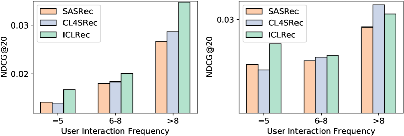
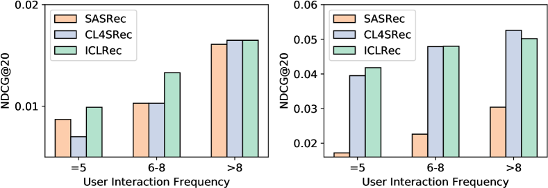
Figure 3. Performance comparison on different user groups among SASRec, CL4SRec and ICLRec (Upper left: Beauty, Upper right: Yelp, Lower left: Sports, Lower right: Toys).)

We also report the model efficiency on Sports. SASRec is the most efficient solution. It spends 3.59 s/epoch on model updates. CL4SRec and the proposed ICLRec spend 6.52 and 11.75 s/epoch, respectively. In detail, ICLRec spends 3.21 seconds to perform intent representation learning, and rest of 8.54 seconds on multi-task learning. The evaluation times of SASRec, CL4SRec, and ICLRec are about the same($\sim$12.72s over testset) since the introduced ICL task is only used during the training stage.

5.3. Robustness Analysis

Robustness w.r.t. user interaction frequency. The user ‘cold-start’ problem (Cai et al., 2021; Yin et al., 2020) is one of the typical data-sparsity issues that recommender systems often face, i.e., most users have limited historical behaviors. To check whether ICL improves the robustness under such a scenario, we split user behavior sequences into three groups based on their behavior sequences’ length, and keep the total number of behavior sequences the same. Models are trained and evaluated on each group of users independently. Figure 3 shows the comparison results on four datasets. We observe that: (1) The proposed ICLRec can consistently performs better than SASRec among all user groups while CL4SRec fails to outperform SASRec in Beauty and Yelp when user behavior sequences are short. This demonstrates that CL4SRec requires individual user behavior sequences long enough to provide ‘complete’ information for auxiliary supervision while ICLRec reduces the need by leveraging user intent information, thus consistently benefiting user representation learning even when users have limited historical interactions. (2) Compared with CL4SRec, we observe that the improvement of ICLRec is mainly because it provides better recommendations to users with low interaction frequency. This verifies that user intent information is beneficial, especially when the recommender system faces data-sparsity issues where information in each individual user sequence is limited.

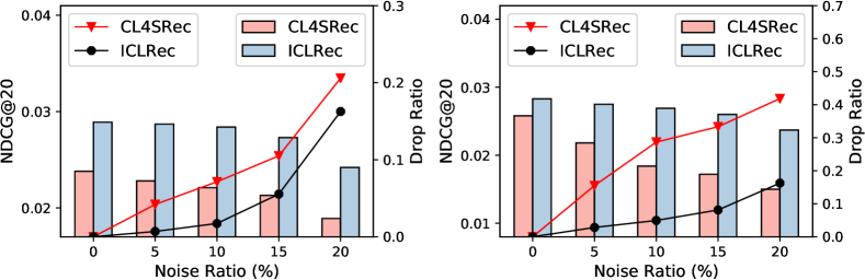
Figure 4. Performance comparison w.r.t. noise ratio on Sports and Yelp. The bar chart shows the performance in NDCG@5 and the line chart shows the corresponding drop rate.

Robustness to Noisy Data. We also conduct experiments on the Sports and Yelp datasets to verify the robustness of ICLRec against noisy interactions in the test phase. Specifically, we randomly add a certain proportion (i.e., 5%, 10%, 15%, 20%) of negative items to text sequences. From Figure 4 we can see that adding noisy data deteriorates the performance of CL4SRec and ICLRec. However, the performance drop ratio of ICLRec is consistently lower than CL4SRec, and its performance with 15% noise proportion can still outperforms CL4SRec without noisy dataset on Sports. The reason might be the leveraged intent information is collaborative information that distilled from all the users. ICL helps the SR model capture semantic structures from user behavior sequences, which increases the robustness of ICLRec to noisy perturbations on individual sequences.

Table 2. Ablation study of ICLRec (NDCG@20).

Model	Dataset
	Sports	Beauty	Toys	Yelp
(A) ICLRec	0.0287	0.0480	0.0554	0.0283
(B) w/o FNM	0.0283	0.0465	0.0524	0.0266
(C) only ICL	0.0263	0.0429	0.0488	0.0267
(D) w/o ICL	0.0238	0.0428	0.0505	0.0258
(E), is (C) w/o seq. aug	0.0242	0.0414	0.0488	0.0213
(F) SASRec	0.0216	0.0387	0.0441	0.0179
(G) ICL + S${}^{3}\text{-Rec}_{ISP}$	0.0157	0.0264	0.0266	0.0205
(H) S${}^{3}\text{-Rec}_{ISP}$	0.0146	0.0198	0.0162	0.0127

5.4. Ablation Study

Our proposed ICLRec contains a novel ICL objective, a false-negative noise mitigation (FNM) strategy, a SeqCL objective, and sequence augmentations. To verify the effectiveness of each component, we conduct an ablation study on four datasets and report results in Table 2. (A) is our final model, and (B) to (F) are ICLRec removed certain components. From (A)-(B) we can see that the FNM leverages the learned intent information to avoid users with similar intents pushing away in their representation space which helps the model to learn better user representations. Compared with (A)-(D), we find that without the proposed ICL, the performance drops significantly, which demonstrates the effectiveness of ICL. Compared with (A)-(C), we find that individual user level mutual information also helps to enhance user representations. As we analyze in Sec. 5.3, it contributes more to long user sequences. Compared with (E)-(F), we find that ICL can perform contrastive SSL without sequence augmentations and outperforms SASRec. While CL4SRec requires the sequence augmentation module to perform contrastive SSL. Comparison between (C) and (E) indicates sequence augmentation enlarges training set, which benefits improving performance.

Since ICL is a model-agostic learning paradigm, we also add ICL to the S${}^{3}\text{-Rec}_{ISP}$ (Zhou et al., 2020) model in the fine-tuning stage to further verify its effectiveness. Results are shown in Table. 2 (G)-(H). We find that the S${}^{3}\text{-Rec}_{ISP}$ model also benefits from the ICL objective. The average improvement over the four datasets is 41.11% in NDCG@20, which further validate the effectiveness and practicality of ICLRec.

5.5. Hyper-parameter Sensitivity

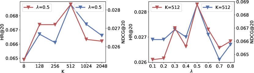
Figure 5. Impact of intent class numbers $K$ and the intent contrastive learning strength $\lambda$ on Yelp.

The larger of the intent class number $K$ means users can have more diverse intentions. The larger value of the strength of SeqCL objective $\beta$ means the ICL task contributes more to the final model. The results on Yelp is shown in Figure 5. We find that: (1) ICLRec reaches its best performance when increasing $K$ to 512, and then it starts to deteriorate as $K$ become larger. When $K$ is very small, the number of users under each intent prototype can potentially be large. As a result, false-positive samples (i.e., users that actually have different intents are considered as having the same intent erroneously) are introduced to the contrastive SSL, thus affecting learning. On the other hand, when $K$ is too large, the number of users under each intent prototype is small, the introduced false-negative samples will also impair contrastive SSL. In Yelp, 512 user intents summarize users’ distinct behaviors best. (2) A ‘sweet-spot’ of $\lambda=0.5$ can also be found. It indicates that the ICL task can benefit the recommendation prediction as an auxiliary task. The impact of the batch size and $\beta$ are provided in Appendix D.

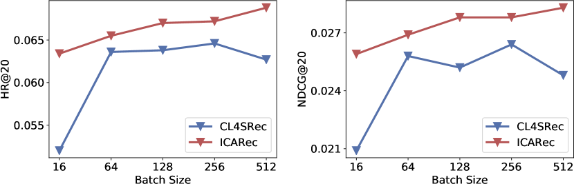
Figure 6. Performance comparison w.r.t. Batch Size.

5.6. Case Study

The Sports dataset (McAuley et al., 2015) contains 2,277 fine-grained item categories, and the Yelp dataset provides 1,001 business categories. We utilize these attributes to study the effectiveness of the proposed ICLRec both quantitatively and qualitatively. Note that we did not use this information during the training phrase. The detailed analysis results are in Appendix E.

6. Conclusion

In this work, we propose a new learning paradigm ICL that can model latent intent factors from user interactions and fuse them into a sequential recommendation model via a new contrastive SSL objective. ICL is formulated within an EM framework, which guarantees convergence. Detailed analyses show the superiority of ICL and experiments conducted on four datasets further demonstrate the effectiveness of the proposed method.

Appendix A Pseudo-code of ICL for SR

Input: training dataset $\left\{s_{u}\right\}_{u=1}^{|\mathcal{U}|}$, sequence encoder $f_{\theta}$, batch size $N$ , hyper-parameters $K$, $\lambda$, $\beta$.

Output: $\theta$.

1 while  $epoch\leq MaxTrainEpoch$ do

       // E-step: Intent Representation Learning

2       $c=Clustering(\left\{f_{\theta}(S^{u})\right\}_{u=1}^{|\mathcal{U}|},K)$

3       Update distribution function $Q(c_{i})=P_{\theta}(c_{i}|S^{u})$

      // M-step: Multi-Task Learning

4       for a minibatch $\{s_{u}\}_{u=1}^{N}$ do

5             for $u\in\{1,2,\cdots,N\}$ do

                   // Construct $2$ views.

6                   $\tilde{S}^{u}_{1}=g_{1}^{u}(S^{u}),\tilde{S}^{u}_{2}=g_{2}^{u}(S^{u}),~{}where~{}g_{1}^{u},g_{2}^{u}\sim\mathcal{G}$

                  // Encoding via $f_{\theta}(\cdot)$

7                  

8                  $\mathbf{h}^{u}=f_{\theta}(S^{u})$

9                   $\mathbf{\tilde{h}}^{u}_{1}=f_{\theta}(\tilde{S}^{u}_{1}),~{}\mathbf{\tilde{h}}^{u}_{2}=f_{\theta}(\tilde{S}^{u}_{2})$

10            

            // Optimization

11             $\mathcal{L}=\mathcal{L}_{\text{NextItem}}+\lambda\cdot\mathcal{L}_{\text{{ICL}}}+\beta\cdot\mathcal{L}_{\text{SeqCL}}$

12             Update network $f_{\theta}(\cdot)$ to minimize $\mathcal{L}$

13      

14

Algorithm 1 ICL for SR

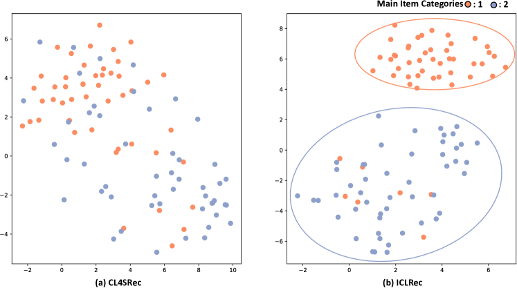
Figure 7. Visualization of the learned users’ representations by CL4SRec and ICLRec on Sports.

Appendix B Proof of Convergence

To proof the convergence of ICL under the generalized EM framework, we just need to proof $P_{\theta^{(m+1)}}(S)\geq P_{\theta^{(m)}}(S)$, where $m$ indicates the number of training iterations. Based on Eq. (7), we have

(19) $$\begin{split}\ln P_{\theta^{(m)}}(S)=\ln\frac{P_{\theta^{(m)}}(S,c_{i})}{P_{\theta^{(m)}}(c_{i}|S)}=\ln P_{\theta^{(m)}}(S,c_{i})-\ln P_{\theta^{(m)}}(c_{i}|S).\end{split}$$

Take the expectation in term of $c$ condition over $S$ on both sides, then we have:

(20) $$\begin{split}\mathbb{E}_{(c|S,\theta^{(m)})}\left[\ln P_{\theta}(S)\right]&=\mathbb{E}_{(c|S,\theta^{(m)})}\left[\ln P_{\theta^{(m)}}(S,c)\right]\\ &-\mathbb{E}_{(c|S,\theta^{(m)})}\left[\ln P_{\theta_{(m)}}(c|S)\right].\end{split}$$

Based on Eq. (12), and 20, the term on left side equal to:

(21) $$\begin{split}\mathbb{E}_{(c|S,\theta^{(m)})}\left[\ln P_{\theta^{(m)}}(S)\right]&=\sum_{i=1}^{K}Q(c_{i})\cdot\ln P_{\theta^{(m)}}(S)=\ln P_{\theta^{(m)}}(S).\end{split}$$

Thus, proof $P_{\theta^{(m+1)}}(S)\geq P_{\theta^{(m)}}(S)$ is equivalent to proof

(22) $$\begin{split}\ln P_{\theta^{(m+1)}}(S)\geq\ln P_{\theta^{(m)}}(S),\end{split}$$

which is equivalent to:

(23) $$\begin{split}\mathbb{E}_{(c|S,\theta^{(m+1)})}\left[\ln P_{\theta^{(m+1)}}(S,c)\right]-\mathbb{E}_{(c|S,\theta^{(m+1)})}\left[\ln P_{\theta_{(m+1)}}(c|S)\right]\\ \geq\mathbb{E}_{(c|S,\theta^{(m)})}\left[\ln P_{\theta^{(m)}}(S,c)\right]-\mathbb{E}_{(c|S,\theta^{(m)})}\left[\ln P_{\theta_{(m)}}(c|S)\right].\end{split}$$

Because we try to optimize $\theta$ at M-step, thus we have

(24) $$\begin{split}\mathbb{E}_{(c|S,\theta^{(m+1)})}\left[\ln P_{\theta^{(m+1)}}(S,c)\right]\geq\mathbb{E}_{(c|S,\theta^{(m)})}\left[\ln P_{\theta^{(m)}}(S,c)\right].\end{split}$$

And based on Jsnson’s inequality, we have

(25) $$\begin{split}\mathbb{E}_{(c|S,\theta^{(m+1)})}\left[\ln P_{\theta_{(m+1)}}(c|S)\right]\leq\mathbb{E}_{(c|S,\theta^{(m)})}\left[\ln P_{\theta_{(m)}}(c|S)\right].\end{split}$$

Combining Eq. (23), (24),and (25), we show that $P_{\theta^{(m+1)}}(S)\geq P_{\theta^{(m)}}(S)$. Thus, the algorithm will converge.

Appendix C Dataset Information

Table 3. Dataset information.

Dataset	Sports	Beauty	Toys	Yelp
$|\mathcal{U}|$	35,598	22,363	19,412	30,431
$|\mathcal{V}|$	18,357	12,101	11,924	20,033
# Actions	0.3m	0.2m	0.17m	0.3m
Avg. length	8.3	8.9	8.6	8.3
Sparsity	99.95%	99.95%	99.93%	99.95%

Appendix D Impact of Batch Size and the strength of SeqCL task $\beta$

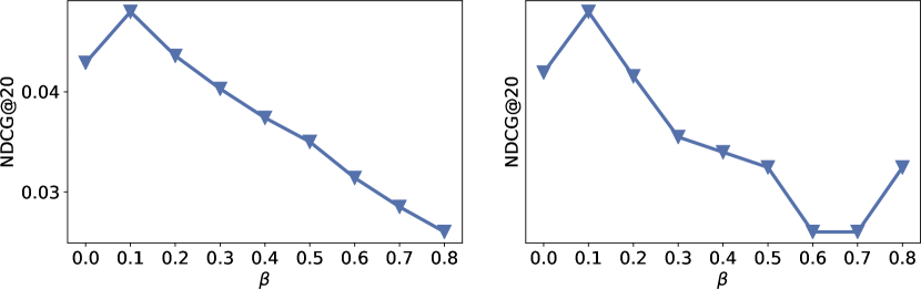
Figure 8. Impact of SeqCL task strength $\beta$ on Beauty (left) and Yelp (right).

Performance w.r.t. batch size on Yelp between CL4SRec and the proposed ICLRec are shown in Figure. 6. We observe that with the batch size increases, CL4SRec’s performance does not continually improve. The reason might because of larger batch sizes introduce false-negative samples, which harms learning. While ICLRec is relatively stable with different batch sizes, and out performs CL4SRec in all circumstances. Because the intent learnt can be seen as a pseudo label of sequences, which helps identify the true positive samples via the proposed contrastive SSL with FNM.

The impact of $\beta$ is shown in Figure 8. We can see that, $\beta$ does help ICLRec improve the performance when it is small (e.g., $\beta\leq 0.1$). However, when $\beta$ continually increase, the model performance drop significantly. This phenomenon also indicates the limitation of SeqCL, since focusing on maximize mutual information between individual sequence pairs may break the global relationships among users.

Table 4. Quantitative Analysis Results. (NDCG@20)

Datasets	SASRec	CL4SRec	ICLRec-A	ICLRec
Sports	0.0216	0.0238	0.0272	0.0275 ($K=2048$)
				0.0287 ($K=1024$)
Yelp	0.0179	0.0258	0.0264	0.0271 ($K=1024$)
				0.0283 ($K=512$)

Appendix E Case Study

Quantitative analysis. We study how ICLRec will perform by considering the item categories of users interacted items as their intents. Specifically, given a user behavior sequence $S^{u}$, we consider the mean of its corresponding trainable item category embeddings as the intent prototype $\mathbf{c}$, aiming to replace the intent representation learning described in Sec. 4.1.2. We run the corresponding model named ICLRec-A and show the comparison results in Table 4. We observe that on Sports (1) ICLRec-A performs better than CL4SRec, which shows the potential benefits of leveraging item category information. (2) ICLRec achieves similar performance as ICLRec-A’s when $K=2048$. Joint analysis with the above qualitative results indicates that ICL can capture meaningful user intents via SSL. (3) ICLRec can outperform ICLRec-A when $K=1024$. We hypothesize that users’ intents can be better described by the latent variables when $K=1024$ thus improving performance. (e.g., parents of the existing item categories.) Similar observations in Yelp.

Qualitative analysis We also compare the proposed ICLRec with CL4SRec by visualizing the learned users’ representations via t-SNE (Van der Maaten and Hinton, 2008). Specifically, we sampled 100 users for whom used to interact with one category of items or the other category. These 100 users also interacted with other categories of items in the past. We visualize the learned users’ representations via t-SNE (Van der Maaten and Hinton, 2008) in Figure 7. From Figure 7 we can see, users’ representations learned by ICLRec intent to pull users that interacted with the same category of items closer to each other while pushing others further away in the representation space than CL4SRec. It reflects that representations learned by ICL can capture more semantic structures, therefore, improves the performance.

References

- (1)
- Cai et al. (2021) Renqin Cai, Jibang Wu, Aidan San, Chong Wang, and Hongning Wang. 2021. Category-aware Collaborative Sequential Recommendation. In Proceedings of the 44th International ACM SIGIR Conference on Research and Development in Information Retrieval. 388–397.
- Caron et al. (2020) Mathilde Caron, Ishan Misra, Julien Mairal, Priya Goyal, Piotr Bojanowski, and Armand Joulin. 2020. Unsupervised learning of visual features by contrasting cluster assignments. arXiv preprint arXiv:2006.09882 (2020).
- Cen et al. (2020) Yukuo Cen, Jianwei Zhang, Xu Zou, Chang Zhou, Hongxia Yang, and Jie Tang. 2020. Controllable multi-interest framework for recommendation. In Proceedings of the 26th ACM SIGKDD International Conference on Knowledge Discovery & Data Mining. 2942–2951.
- Chen et al. (2020) Ting Chen, Simon Kornblith, Mohammad Norouzi, and Geoffrey Hinton. 2020. A simple framework for contrastive learning of visual representations. In International conference on machine learning. PMLR, 1597–1607.
- Chen et al. (2021) Yongjun Chen, Jia Li, Chenghao Liu, Chenxi Li, Markus Anderle, Julian McAuley, and Caiming Xiong. 2021. Modeling Dynamic Attributes for Next Basket Recommendation. arXiv preprint arXiv:2109.11654 (2021).
- Fan et al. (2021) Ziwei Fan, Zhiwei Liu, Jiawei Zhang, Yun Xiong, Lei Zheng, and Philip S. Yu. 2021. Continuous-Time Sequential Recommendation with Temporal Graph Collaborative Transformer. In Proceedings of the 30th ACM International Conference on Information and Knowledge Management. ACM.
- Gao et al. (2021) Tianyu Gao, Xingcheng Yao, and Danqi Chen. 2021. SimCSE: Simple Contrastive Learning of Sentence Embeddings. arXiv preprint arXiv:2104.08821 (2021).
- Gunel et al. (2020) Beliz Gunel, Jingfei Du, Alexis Conneau, and Ves Stoyanov. 2020. Supervised contrastive learning for pre-trained language model fine-tuning. arXiv preprint arXiv:2011.01403 (2020).
- He et al. (2020b) Kaiming He, Haoqi Fan, Yuxin Wu, Saining Xie, and Ross Girshick. 2020b. Momentum contrast for unsupervised visual representation learning. In Proceedings of the IEEE/CVF Conference on Computer Vision and Pattern Recognition. 9729–9738.
- He and McAuley (2016) Ruining He and Julian McAuley. 2016. Fusing similarity models with markov chains for sparse sequential recommendation. In 2016 IEEE 16th International Conference on Data Mining (ICDM). IEEE, 191–200.
- He et al. (2020a) Xiangnan He, Kuan Deng, Xiang Wang, Yan Li, Yongdong Zhang, and Meng Wang. 2020a. Lightgcn: Simplifying and powering graph convolution network for recommendation. In Proceedings of the 43rd International ACM SIGIR conference on research and development in Information Retrieval. 639–648.
- Hidasi et al. (2015) Balázs Hidasi, Alexandros Karatzoglou, Linas Baltrunas, and Domonkos Tikk. 2015. Session-based recommendations with recurrent neural networks. arXiv preprint arXiv:1511.06939 (2015).
- Kang and McAuley (2018) Wang-Cheng Kang and Julian McAuley. 2018. Self-attentive sequential recommendation. In ICDM. IEEE, 197–206.
- Khosla et al. (2020) Prannay Khosla, Piotr Teterwak, Chen Wang, Aaron Sarna, Yonglong Tian, Phillip Isola, Aaron Maschinot, Ce Liu, and Dilip Krishnan. 2020. Supervised contrastive learning. arXiv preprint arXiv:2004.11362 (2020).
- Kingma and Ba (2014) Diederik P Kingma and Jimmy Ba. 2014. Adam: A method for stochastic optimization. arXiv preprint arXiv:1412.6980 (2014).
- Krichene and Rendle (2020) Walid Krichene and Steffen Rendle. 2020. On Sampled Metrics for Item Recommendation. In SIGKDD. 1748–1757.
- Li et al. (2019) Chao Li, Zhiyuan Liu, Mengmeng Wu, Yuchi Xu, Huan Zhao, Pipei Huang, Guoliang Kang, Qiwei Chen, Wei Li, and Dik Lun Lee. 2019. Multi-interest network with dynamic routing for recommendation at Tmall. In Proceedings of the 28th ACM International Conference on Information and Knowledge Management. 2615–2623.
- Li et al. (2021b) Haoyang Li, Xin Wang, Ziwei Zhang, Jianxin Ma, Peng Cui, and Wenwu Zhu. 2021b. Intention-aware Sequential Recommendation with Structured Intent Transition. IEEE Transactions on Knowledge and Data Engineering (2021).
- Li et al. (2020a) Jiacheng Li, Yujie Wang, and Julian McAuley. 2020a. Time Interval Aware Self-Attention for Sequential Recommendation. In WSDM. 322–330.
- Li et al. (2020b) Junnan Li, Pan Zhou, Caiming Xiong, and Steven CH Hoi. 2020b. Prototypical contrastive learning of unsupervised representations. arXiv preprint arXiv:2005.04966 (2020).
- Li et al. (2021a) Yang Li, Tong Chen, Peng-Fei Zhang, and Hongzhi Yin. 2021a. Lightweight Self-Attentive Sequential Recommendation. In Proceedings of the 30th ACM International Conference on Information & Knowledge Management. 967–977.
- Liu et al. (2021c) Xiao Liu, Fanjin Zhang, Zhenyu Hou, Li Mian, Zhaoyu Wang, Jing Zhang, and Jie Tang. 2021c. Self-supervised learning: Generative or contrastive. IEEE Transactions on Knowledge and Data Engineering (2021).
- Liu et al. (2021a) Zhiwei Liu, Yongjun Chen, Jia Li, Philip S Yu, Julian McAuley, and Caiming Xiong. 2021a. Contrastive self-supervised sequential recommendation with robust augmentation. arXiv preprint arXiv:2108.06479 (2021).
- Liu et al. (2021b) Zhiwei Liu, Ziwei Fan, Yu Wang, and Philip S Yu. 2021b. Augmenting Sequential Recommendation with Pseudo-Prior Items via Reversely Pre-training Transformer. arXiv preprint arXiv:2105.00522 (2021).
- Liu et al. (2020a) Zhiwei Liu, Xiaohan Li, Ziwei Fan, Stephen Guo, Kannan Achan, and S Yu Philip. 2020a. Basket recommendation with multi-intent translation graph neural network. In 2020 IEEE International Conference on Big Data (Big Data). IEEE, 728–737.
- Liu et al. (2020b) Zhiwei Liu, Lin Meng, Jiawei Zhang, and Philip S Yu. 2020b. Deoscillated Graph Collaborative Filtering. arXiv preprint arXiv:2011.02100 (2020).
- Ma et al. (2020) Jianxin Ma, Chang Zhou, Hongxia Yang, Peng Cui, Xin Wang, and Wenwu Zhu. 2020. Disentangled self-supervision in sequential recommenders. In Proceedings of the 26th ACM SIGKDD International Conference on Knowledge Discovery & Data Mining. 483–491.
- McAuley et al. (2015) Julian McAuley, Christopher Targett, Qinfeng Shi, and Anton Van Den Hengel. 2015. Image-based recommendations on styles and substitutes. In SIGIR. 43–52.
- Mnih and Kavukcuoglu (2013) Andriy Mnih and Koray Kavukcuoglu. 2013. Learning word embeddings efficiently with noise-contrastive estimation. In Advances in neural information processing systems. 2265–2273.
- Oord et al. (2018) Aaron van den Oord, Yazhe Li, and Oriol Vinyals. 2018. Representation learning with contrastive predictive coding. arXiv preprint arXiv:1807.03748 (2018).
- Pan et al. (2020) Zhiqiang Pan, Fei Cai, Yanxiang Ling, and Maarten de Rijke. 2020. An intent-guided collaborative machine for session-based recommendation. In Proceedings of the 43rd International ACM SIGIR Conference on Research and Development in Information Retrieval. 1833–1836.
- Rendle (2010) Steffen Rendle. 2010. Factorization machines. In 2010 IEEE International conference on data mining. IEEE, 995–1000.
- Rendle et al. (2012) Steffen Rendle, Christoph Freudenthaler, Zeno Gantner, and Lars Schmidt-Thieme. 2012. BPR: Bayesian personalized ranking from implicit feedback. arXiv preprint arXiv:1205.2618 (2012).
- Rendle et al. (2010) Steffen Rendle, Christoph Freudenthaler, and Lars Schmidt-Thieme. 2010. Factorizing personalized markov chains for next-basket recommendation. In Proceedings of the 19th international conference on World wide web. 811–820.
- Sun et al. (2019) Fei Sun, Jun Liu, Jian Wu, Changhua Pei, Xiao Lin, Wenwu Ou, and Peng Jiang. 2019. BERT4Rec: Sequential recommendation with bidirectional encoder representations from transformer. In CIKM. 1441–1450.
- Tang and Wang (2018) Jiaxi Tang and Ke Wang. 2018. Personalized top-n sequential recommendation via convolutional sequence embedding. In WSDM. 565–573.
- Tanjim et al. (2020) Md Mehrab Tanjim, Congzhe Su, Ethan Benjamin, Diane Hu, Liangjie Hong, and Julian McAuley. 2020. Attentive sequential models of latent intent for next item recommendation. In Proceedings of The Web Conference 2020. 2528–2534.
- Taylor (1953) Wilson L Taylor. 1953. “Cloze procedure”: A new tool for measuring readability. Journalism quarterly 30, 4 (1953), 415–433.
- Van der Maaten and Hinton (2008) Laurens Van der Maaten and Geoffrey Hinton. 2008. Visualizing data using t-SNE. Journal of machine learning research 9, 11 (2008).
- Vaswani et al. (2017) Ashish Vaswani, Noam Shazeer, Niki Parmar, Jakob Uszkoreit, Llion Jones, Aidan N Gomez, Łukasz Kaiser, and Illia Polosukhin. 2017. Attention is all you need. In Advances in neural information processing systems. 5998–6008.
- Wang et al. (2019b) Shoujin Wang, Liang Hu, Yan Wang, Quan Z Sheng, Mehmet Orgun, and Longbing Cao. 2019b. Modeling multi-purpose sessions for next-item recommendations via mixture-channel purpose routing networks. In International Joint Conference on Artificial Intelligence. International Joint Conferences on Artificial Intelligence.
- Wang et al. (2019a) Xiang Wang, Xiangnan He, Meng Wang, Fuli Feng, and Tat-Seng Chua. 2019a. Neural graph collaborative filtering. In Proceedings of the 42nd international ACM SIGIR conference on Research and development in Information Retrieval. 165–174.
- Wu et al. (2017) Chao-Yuan Wu, Amr Ahmed, Alex Beutel, Alexander J Smola, and How Jing. 2017. Recurrent recommender networks. In Proceedings of the tenth ACM international conference on web search and data mining. 495–503.
- Wu et al. (2021) Jiancan Wu, Xiang Wang, Fuli Feng, Xiangnan He, Liang Chen, Jianxun Lian, and Xing Xie. 2021. Self-supervised graph learning for recommendation. In Proceedings of the 44th International ACM SIGIR Conference on Research and Development in Information Retrieval. 726–735.
- Xie et al. (2020) Xu Xie, Fei Sun, Zhaoyang Liu, Shiwen Wu, Jinyang Gao, Bolin Ding, and Bin Cui. 2020. Contrastive Learning for Sequential Recommendation. arXiv preprint arXiv:2010.14395 (2020).
- Yan et al. (2019) An Yan, Shuo Cheng, Wang-Cheng Kang, Mengting Wan, and Julian McAuley. 2019. CosRec: 2D convolutional neural networks for sequential recommendation. In Proceedings of the 28th ACM International Conference on Information and Knowledge Management. 2173–2176.
- Yao et al. (2020) Tiansheng Yao, Xinyang Yi, Derek Zhiyuan Cheng, Felix Yu, Ting Chen, Aditya Menon, Lichan Hong, Ed H Chi, Steve Tjoa, Jieqi Kang, et al. 2020. Self-supervised Learning for Large-scale Item Recommendations. arXiv preprint arXiv:2007.12865 (2020).
- Yin et al. (2020) Jianwen Yin, Chenghao Liu, Weiqing Wang, Jianling Sun, and Steven CH Hoi. 2020. Learning transferrable parameters for long-tailed sequential user behavior modeling. In Proceedings of the 26th ACM SIGKDD International Conference on Knowledge Discovery & Data Mining. 359–367.
- Zhang and McAuley (2020) Hengrui Zhang and Julian McAuley. 2020. Stacked Mixed-Order Graph Convolutional Networks for Collaborative Filtering. In Proceedings of the 2020 SIAM International Conference on Data Mining. SIAM, 73–81.
- Zhang et al. (2020) Yan Zhang, Ruidan He, Zuozhu Liu, Kwan Hui Lim, and Lidong Bing. 2020. An unsupervised sentence embedding method by mutual information maximization. arXiv preprint arXiv:2009.12061 (2020).
- Zhou et al. (2020) Kun Zhou, Hui Wang, Wayne Xin Zhao, Yutao Zhu, Sirui Wang, Fuzheng Zhang, Zhongyuan Wang, and Ji-Rong Wen. 2020. S3-rec: Self-supervised learning for sequential recommendation with mutual information maximization. In Proceedings of the 29th ACM International Conference on Information & Knowledge Management. 1893–1902.
- Zhou et al. (2021) Yao Zhou, Jianpeng Xu, Jun Wu, Zeinab Taghavi, Evren Korpeoglu, Kannan Achan, and Jingrui He. 2021. PURE: Positive-Unlabeled Recommendation with Generative Adversarial Network. In Proceedings of the 27th ACM SIGKDD Conference on Knowledge Discovery & Data Mining. 2409–2419.