The LVS Parametric Tadpole Constraint

Abstract

The large volume scenario (LVS) for de Sitter compactifications of the type IIB string is, at least in principle, well protected from various unknown corrections. The reason is that, by construction, the Calabi-Yau volume is exponentially large. However, as has recently been emphasised, in practice the most explicit models are rather on the border of parametric control. We identify and quantify parametrically what we believe to be the main issue behind this difficulty. Namely, a large volume implies a shallow AdS minimum and hence a small uplift. The latter, if it relies on an anti-D3 in a throat, requires a large negative tadpole. As our main result, we provide a simple and explicit formula for what this tadpole has to be in order to control the most dangerous corrections. The fundamental ingredients are parameters specifying the desired quality of control. We comment on the interplay between our constraint and the tadpole conjecture. We also discuss directions for future work which could lead to LVS constructions satisfying the tadpole constraint with better control, as well as further challenges that may exist for the LVS. Our formula then represents a very concrete challenge for future searches for and the understanding of relevant geometries.

1 Introduction

The construction of metastable de Sitter vacua in string theory is challenging and, in spite of many years of work, the focus has remained on two close cousins: the KKLT Kachru:2003aw and the LVS Balasubramanian:2005zx proposals. Recently, fundamental doubts about the very existence of de Sitter space in quantum gravity (see e.g. Danielsson:2018ztv ; Obied:2018sgi ; Garg:2018reu ; Ooguri:2018wrx ) have triggered intense scrutiny of these models. KKLT has arguably survived attacks related to the stability question of the anti-D3 uplift Bena:2009xk ; Bena:2011wh ; Michel:2014lva ; Blaback:2019ucp and the gaugino condensate Moritz:2017xto ; Carta:2019rhx ; Gautason:2019jwq ; Hamada:2019ack ; Kachru:2019dvo ; Hamada:2021ryq . It is too early to judge how it will fare in view of the singular-bulk problem Gao:2020xqh , which arises since one is forced to glue a large throat into a fairly small Calabi-Yau Carta:2019rhx . In view of this uncertainty (see Carta:2021lqg ; Demirtas:2021nlu for some the recent discussion), it is maybe natural to shift the focus on the LVS, where the singular-bulk problem does, at first sight, not arise Gao:2020xqh because the volume can be made exponentially large.

However, as recently emphasised in Junghans:2022exo , the problem does not entirely disappear either. The reason is that at large volume the AdS minimum of the LVS becomes shallow, requiring a small uplift and hence a strongly warped throat. The latter comes with a large positive D3 charge and hence requires a large negative D3 charge of the embedding Calabi-Yau orientifold. This requirement has been emphasised as a potential problem in Bena:2020xrh and argued to be a solvable issue in Crino:2020qwk , where the focus was on a concrete model. Most recently, this model has in turn been challenged in Junghans:2022exo on the basis that all the different corrections can not be made sufficiently small at the same time.

Our purpose in this short note is to derive a simple formula quantifying what we believe to be the most serious obstacle to defending the LVS against such skepticism. We call our result the ‘LVS parametric tadpole constraint’, as it quantifies the amount of negative tadpole which the geometry must possess to be in perturbative control. The desired quality of control is an input to this formula.

Our result will follow from two different corrections to the LVS potential, both with the same parametric behaviour. One is related to warping and hence similar in spirit to the singular-bulk problem, the other to higher $F$-terms deAlwis:2005tg ; Cicoli:2013swa ; Ciupke:2015msa . As we will see, this leads to a simple, strong and conceptually clear bound on controlled LVS models with de Sitter uplift, deriving from the requirement to keep warping and higher $F$-term effects small at the same time. By comparison, the recent analysis of Junghans:2022exo used these conditions together with a number of conditions related to further corrections (see e.g. Conlon:2010ji ; Antoniadis:2019rkh ; Conlon:2009kt ; Weissenbacher:2019mef ; Grimm:2013bha ; Grimm:2015mua ; Junghans:2014zla ; vonGersdorff:2005bf ; Berg:2005ja ; Berg:2007wt ; Cicoli:2007xp ; Cicoli:2008va ; Burgess:2020qsc ; Cicoli:2021rub ; Minasian:2015bxa ) to collectively constrain the LVS. These analytical constraints were then applied to a specific Calabi-Yau orientifold. The most important of those further corrections are probably certain logarithmic contributions to the Kahler potential, which are not yet unambiguously established. We will comment on this in slightly more detail below. Many of the remaining corrections are interesting but probably not as dangerous. We will discuss them only briefly in what follows.

We note that in Gao:2022uop we provide a general discussion of loop corrections to the Kahler moduli Kahler potential in type-IIB compactifications vonGersdorff:2005bf ; Berg:2005ja ; Berg:2007wt ; Cicoli:2007xp ; Cicoli:2008va . We will in particular discuss at which order in $\alpha^{\prime}$, $g_{s}$, and cycle volumes loop corrections can appear and what their potential impact on proposed compactifications, such as the LVS, is.

The rest of the present paper is organized as follows: We list the most important LVS relations in Sect. 2, we derive the proposed key equation for the required minimal tadpole in Sect. 3. Then, in Sect. 4, we discuss how one may try to strengthen the LVS proposal in the future in spite of the presented constraint. We also discuss further challenges and comment on the interplay of our constraint with the tadpole conjecture Bena:2020xrh ; Bena:2021wyr ; Plauschinn:2021hkp ; Lust:2021xds ; Bena:2021qty .

2 Summary of basic equations

To set the scene, we recall the LVS set-up. One compactifies IIB string theory to 4D on a Calabi-Yau orientifold $X$ with flux and warping. The geometry has at least a big 4-cycle $\tau_{b}$ and a small 4-cycle $\tau_{s}$. The corresponding Kahler potential reads Balasubramanian:2005zx ; Becker:2002nn

$$K=-2\ln\left(\mathcal{V}+\frac{\xi}{2g_{s}^{3/2}}\right)=-2\ln\left(\tau_{b}^{3/2}-\kappa_{s}\tau_{s}^{3/2}-\frac{\chi\,\zeta(3)}{4(2\pi)^{3}g_{s}^{3/2}}\right)\,.$$ (2.1)

Here ${\cal V}=\tau_{b}^{3/2}-\kappa_{s}\tau_{s}^{3/2}$ is the Calabi-Yau volume in units of $l_{s}=2\pi\sqrt{\alpha^{\prime}}$ and after a rescaling to the 10d Einstein frame. The constant $\kappa_{s}$ is related to the triple intersection number of $\tau_{s}$ and an analogous constant in front of $\tau_{b}$ has been absorbed by rescaling $\tau_{b}$. The string coupling is $g_{s}$ and $\chi$ is the Euler number of the Calabi-Yau. The superpotential is given by

$$W=W_{0}+A_{s}\text{e}^{-a_{s}T_{s}}\,,$$ (2.2)

with $W_{0}$ due to flux and the nonperturbative correction coming from either ED3-branes ($a_{s}=2\pi$) or gaugino condensation on D7-branes ($a_{s}$ depends on the gauge group, e.g. $a_{s}=\pi/3$ for $SO(8)$). The prefactor $A_{s}$ is model-dependent. We have absorbed the complex structure Kahler potential in a multiplicative rescaling of $W_{0}$ and $A_{s}$.

This yields the pure LVS scalar potential (in 4d Planck units)

$$V=\frac{4a_{s}^{2}|A_{s}|^{2}g_{s}\sqrt{\tau_{s}}\text{e}^{-2a_{s}\tau_{s}}}{3\kappa_{s}\mathcal{V}}-\frac{2a_{s}|A_{s}|g_{s}\tau_{s}|W_{0}|\text{e}^{-a_{s}\tau_{s}}}{\mathcal{V}^{2}}+\frac{3\xi|W_{0}|^{2}}{8\sqrt{g_{s}}\mathcal{V}^{3}}\,,$$ (2.3)

which is minimized by

$$\mathcal{V}=\frac{3\kappa_{s}|W_{0}|\sqrt{\tau_{s}}}{4a_{s}|A_{s}|}\text{e}^{a_{s}\tau_{s}}\,\,\,,\qquad\qquad\tau_{s}=\frac{\xi^{2/3}}{(2\kappa_{s})^{2/3}g_{s}}+\mathcal{O}(1)\,,$$ (2.4)

leading to an AdS vacuum at

$$V_{\text{AdS}}=-\frac{3\kappa_{s}g_{s}\sqrt{\tau_{s}}|W_{0}|^{2}}{8a_{s}\mathcal{V}^{3}}\,.$$ (2.5)

As noted in the Appendix of Hebecker:2012aw this value is parametrically suppressed with respect to the individual terms in $V$ by a factor of $1/\tau_{s}$ or $g_{s}$. This has been emphasised and studied in detail in Junghans:2022exo under the name ‘non-perturbative no-scale structure’.

One now assumes that a Klebanov-Strassler throat is present and places an anti-D3 brane at its tip. This adds a metastable uplift Kachru:2003aw

$$V_{\text{uplift}}=V_{\overline{D3}}=2T_{D3}e^{4A(0)}$$ (2.6)

to the scalar potential. Here $T_{D3}$ is the D3-brane tension in 4D Einstein frame and $e^{A(0)}$ is the warp factor at the tip of the throat. To determine this warp factor, we neglect the difficult issue of backreaction Bena:2018fqc ; Blumenhagen:2019qcg since it is expected to make the uplift smaller. Hence we are being conservative by disregarding it. We rather use the standard Klebanov-Strassler geometry, glued into the conical region of a compact Calabi-Yau. We are careful to keep all ${\cal O}(1)$ factors except for those which are unknown since they are related to the specific Calabi-Yau (cf. App. A for details). Including in particular the corrected volume scaling of Kachru:2003sx , we find

$$e^{4A(0)}=\left(\frac{g_{s}^{3/2}\mathcal{V}}{\mathcal{V}_{0}}\right)^{2/3}\frac{3\,2^{2/3}\pi}{a_{0}}\,\frac{N}{g_{s}M^{2}}e^{-\frac{8\pi K}{3g_{s}M}}\,.$$ (2.7)

Here $a_{0}\approx 0.71805$ is a numerical constant related to the explicit Klebanov-Strassler geometry Klebanov:2000hb , $\mathcal{V}_{0}$ is the volume of the $T^{1,1}$ where the conifold is glued into the Calabi-Yau, and $M$ is the $F_{3}$ and $K$ the $H_{3}$ flux on the throat 3-cycles. The contribution of the flux in the throat to the D3-tadpole is $N=KM$. The final form of the uplift potential is then

$$V_{\text{uplift}}=\frac{\left(3^{2}\,\pi^{3}\,2^{22/3}\right)^{1/5}}{a_{0}}\frac{\text{e}^{-\frac{8\pi K}{3g_{s}M}}}{g_{s}M^{2}\mathcal{V}^{4/3}}\,.$$ (2.8)

Jumping slightly ahead we note that the weaker volume suppression of the uplift as compared to the depth of the AdS potential in (2.5) does not represent a problem. The matching of the two effects will be ensured by the non-trivial volume scaling of $|W_{0}|^{2}$ and of the exponential warping suppression in (2.8).

Before moving on to the derivation of the tadpole constraint, we have to discuss one of the so-called higher $F$-term corrections. It is important since it bounds the size of $W_{0}$ in terms of the Calabi-Yau volume. Concretely, this correction comes from eight derivative terms involving the field strength $G_{3}$ and takes the form Ciupke:2015msa ; Junghans:2022exo

$$\delta V_{F}\sim\frac{W_{0}^{4}g_{s}^{1/2}}{\mathcal{V}^{11/3}}\,.$$ (2.9)

Its ratio to the value of the AdS potential at the minimum (2.5) is required to be small. To quantify this, we multiply this ratio by our control parameter $c_{W_{0}}$ and set the result equal to unity:

$$1=c_{W_{0}}\frac{16a_{s}}{3(2\kappa_{s})^{2/3}\xi^{1/3}}\,\frac{W_{0}^{2}}{\mathcal{V}^{2/3}}\,.$$ (2.10)

For $c_{W_{0}}\gg 1$, higher terms in the superspace derivative expansion are suppressed deAlwis:2005tg ; Cicoli:2013swa ; Ciupke:2015msa .

Let us briefly comment on the actual prefactor in (2.9). In Ciupke:2015msa the correction is determined to be $V_{F}=\hat{\lambda}W_{0}^{4}g_{s}^{1/2}\,\Pi_{i}\,t^{i}/\mathcal{V}^{4}$ where $t^{i}$ is some 2-cycle volume, $|\hat{\lambda}|$ can roughly be estimated to be of order $|\xi/\chi|\sim 10^{-3}$, and $\Pi_{i}$ are topological numbers estimated to be of $\mathcal{O}(10-100)$. The topological numbers can be computed in explicit examples Ciupke:2015msa ; Cicoli:2016xae ; Cicoli:2017axo . Note that in (2.9) we focused on the contribution of the largest 2-cycle $t_{\ast}\sim\mathcal{V}^{1/3}$.

3 The LVS Parametric Tadpole Constraint

The LVS tadpole constraint is derived in two steps: First, we require the uplift potential (2.8) to be of the size of the potential in the AdS minimum (2.5). This leads to

$$\mathcal{V}=\frac{a_{0}}{(3^{2}\pi^{3}2^{22/3})^{1/5}}\left(\frac{3(2\kappa_{s})^{2/3}\xi^{1/3}}{16a_{s}}\right)^{2}\frac{g_{s}^{1/2}}{c_{W_{0}}}g_{s}M^{2}\,\text{e}^{\frac{8\pi}{3g_{s}M^{2}}N}\,,$$ (3.1)

where we replaced $|W_{0}|$ by (2.10). Setting $\mathcal{V}$ in (2.4) equal to (3.1) gives an implicit equation for $\tau_{s}=\tau_{s}(N)$ which can be solved to leading order by comparing the exponentials:

$$a_{s}\tau_{s}=\frac{16\pi N}{9g_{s}M^{2}}+\ln(\mathcal{O}(1))\,.$$ (3.2)

In the second step, we bound the volume from below by demanding that we have a well-controlled solution. One argument is to require that the singular-bulk problem is avoided. This imposes Gao:2020xqh ; Carta:2019rhx

$$1\gg\frac{N}{\mathcal{V}^{2/3}}\,.$$ (3.3)

However, as recently argued in Junghans:2022exo , a related and more quantitative bound can be given by studying 10d higher-curvature terms. Indeed, before strong warping leads to the formation of singular regions, it drives curvature corrections large. Specifically, consider a correction to the 4d Einstein-Hilbert term, analogous to BBHL Becker:2002nn , arising from the interplay between the 10d $R_{10}^{4}$ term and a varying warp factor Junghans:2022exo :

One uses the warped metric ansatz

$$\mathrm{d}s^{2}=\text{e}^{2A(y)}g_{\mu\nu}\mathrm{d}x^{\mu}\mathrm{d}x^{\nu}+\text{e}^{-2A(y)}\tilde{g}_{mn}\mathrm{d}y^{m}\mathrm{d}y^{n}$$ (3.4)

together with the term

$$\frac{1}{g_{s}^{3/2}}\int\mathrm{d}^{10}x\sqrt{-G}\varepsilon^{ABM_{1}\dots M_{8}}\varepsilon_{ABN_{1}\dots N_{8}}R^{N_{1}N_{2}}_{~{}~{}~{}~{}~{}M_{1}M_{2}}\cdots R^{N_{7}N_{8}}_{~{}~{}~{}~{}~{}M_{7}M_{8}}$$ (3.5)

from the $R^{4}_{10}$ correction to the type-IIB action Becker:2002nn ; Antoniadis:1997eg in 10d Einstein frame. To derive the contribution to the 4d Einstein-Hilbert term, we focus on fluctuations of the type $g_{\mu\nu}=g_{\mu\nu}(x)$. We also disregard terms with derivatives of $A(y)$. This turns (3.5) into

$$\frac{1}{g_{s}^{3/2}}\int_{\mathcal{M}_{10}}e^{2A(y)}R\wedge R\wedge R\wedge R\wedge e\wedge e\,,$$ (3.6)

where $R$ is the Riemann tensor of the unwarped Calabi-Yau compactification with metric $(g_{\mu\nu},\tilde{g}_{mn})$ and $e$ denotes the vielbein 1-form. Since we are now working with a product geometry, the contribution to the 4d Einstein-Hilbert term can be made explicit as

$$\frac{1}{g_{s}^{3/2}}\int\mathrm{d}^{4}xR_{4}\int_{X}R_{6}\wedge R_{6}\wedge R_{6}\,\Big{(}1+(\text{e}^{2A(y)}-1)\Big{)}$$

$$\approx \frac{1}{g_{s}^{3/2}}\int d^{4}xR_{4}\left(\chi(X)+\frac{\chi(X)N}{\mathcal{V}^{2/3}}\right).$$ (3.7)

Here we assumed that the bulk of the Calabi-Yau is at weak warping, $e^{2A}\simeq 1$. We may then use the fact that, in the 10d string frame, $(e^{-4A}-1)$ is the solution of a Poisson equation with the sources being the throat-localised flux $\sim g_{s}N$ and the compensating negative tadpole elsewhere in the compact space. The 6d Greens function behaviour $\sim 1/r^{4}$ then implies that the typical variations of $(e^{-4A}-1)$ and hence of $(e^{2A}-1)$ on the scale of the Calabi-Yau are $\sim g_{s}N/r^{4}\sim N/\mathcal{V}^{2/3}$.

We deviate from Junghans:2022exo in that we expect a scaling of the warping correction term with the Euler number $\chi(X)$. The reason is that we assume a slowly varying warp factor Gao:2020xqh and hence do not expect a parametrically strong cancellation between the contributions from different regions.

The correction to the Einstein-Hilbert term then translates into a Kahler potential correction and, analogously to the $\alpha^{\prime}$ effect in the last term of (2.3), to a correction to the scalar potential:

$$\delta V=\frac{15\,\xi\,N\,|W_{0}|^{2}}{8\sqrt{g_{s}}\,\mathcal{V}^{11/3}}\,\mathcal{O}(1)\,.$$ (3.8)

This correction in turn corrects the value of the (A)dS minimum and the stability condition of the dS minimum Junghans:2022exo . We focus on the effect on the value of the potential at the minimum since the stability of the minimum depends crucially on the unknown sign of the correction (3.8). A measure for parametric control is given by comparing the size of the correction to the scalar potential (3.8) and its value at the minimum (2.5). Hence, we are prompted to consider the following improved version of (3.3):

$$1=c_{N}\frac{10\,a_{s}\,\xi^{2/3}}{(2\kappa_{s})^{2/3}g_{s}}\frac{N}{\mathcal{V}^{2/3}}\,.$$ (3.9)

A large control parameter $c_{N}\gg 1$ again ensures a parametric suppression of the correction compared to the leading term.

Now, we require the volume in (3.9) to be equal to (3.1) and replace subsequently $g_{s}$ by $\tau_{s}$ using (2.4). In doing so, we leave the combination $g_{s}M^{2}$ untouched since it represents an important parameter characterising the metastability of the throat. This leads to an equation for $N$ which is of the form $w\text{e}^{w}=x$, where

$$w=-\frac{16\pi}{21g_{s}M^{2}}N\,,\quad\quad x=-\frac{3^{3/5}\pi^{9/35}\,a_{0}^{2/7}}{14\,\,2^{2/15}\,5^{3/7}}\frac{\kappa_{s}^{2/7}\,\xi^{2/7}}{a_{s}^{3/7}\,c_{W_{0}}^{2/7}\,c_{N}^{3/7}}\frac{1}{(g_{s}M^{2})^{1/7}}\,.$$ (3.10)

An equation of the above type is solved by $w=\mathcal{W}_{-1}(x)$, where $\mathcal{W}_{-1}(x)$ is a branch of the Lambert $\mathcal{W}$ function. We find the exact result

$$N=-\frac{21g_{s}M^{2}}{16\pi}\mathcal{W}_{-1}(x)=-\frac{21g_{s}M^{2}}{16\pi}\biggl{(}\ln(-x)+\ln(-\ln(-x))+\mathcal{O}(1)\biggr{)}\,,$$ (3.11)

where we expanded $\mathcal{W}_{-1}(x)$ around $x=0$. In order for the D3-tadpole in our compactification to cancel, we must at least have sufficient negative tadpole $Q_{3}$ from O3/O7-planes and D7-branes to cancel the flux in the throat

$$-Q_{3}>N\,.$$ (3.12)

In addition to (3.12), there is another lower bound on $-Q_{3}$ given by Denef:2004ze

$$-Q_{3}\geq 4\pi\frac{g_{s}W_{0}^{2}}{2}\,,$$ (3.13)

where the $4\pi$ arises since our superpotential $W$ is normalized differently compared to Denef:2004ze . Expressing $W_{0}$ by (2.10) and subsequently $\mathcal{V}$ by (3.9) we find

$$-Q_{3}\geq\frac{c_{N}}{c_{W_{0}}}\frac{15\pi\xi}{4}N\equiv c_{Q}N\,.$$ (3.14)

Our main result is then that by filling in (3.11) for $N$ in (3.12) and (3.14), we obtain two lower bounds on the D3-tadpole. For any given model and two prescribed values $c_{N}$ and $c_{W_{0}}$, we should check that the strongest of these bounds is satisfied.

This result allows for a more compact formulation if we do not fix $c_{N}$ and $c_{W_{0}}$ but merely restrict them such that some minimal quality of control is ensured. Specifically, we demand $c_{N}\geq c_{N,{\rm min}}$ and $c_{W_{0}}\geq c_{W_{0},{\rm min}}$, assuming also that the two values $c_{N,{\rm min}}$ and $c_{W_{0},{\rm min}}$ are comparable. This is illustrated in Fig. 1, where the grey area represents the forbidden regime. The blue line in the plot separates the regimes where one or the other of the two bounds is stronger. It is described by $c_{W_{0}}/c_{N}=15\pi\xi/4$ or, equivalently, $c_{Q}=1$. Since $15\pi\xi/4$ is in general significantly larger than unity, the blue line cuts the horizontal rather than the vertical part of the boundary between the grey and white area.

Over the white part of the plot in Fig. 1, we have a function $-Q_{3}^{*}(c_{N},c_{W_{0}})$ given by the r.h. side of (3.12) or (3.14), whichever is largest. For a conservative constraint, we want to know the minimal value of that function. To determine this value, we first consider the area to the right of the blue line, where $c_{Q}<1$. It is immediately clear from eqs. (3.10)-(3.12) that, as indicated by the arrows, our function $-Q_{3}^{*}(c_{N},c_{W_{0}})$ falls as we move to smaller $c_{W_{0}}$ at fixed $c_{N}$. Hence the minimum is attained on the blue line or to its left. On the contrary, in the region left of the blue line, i.e. for $c_{Q}>1$, the value of $-Q_{3}^{*}(c_{N},c_{W_{0}})$ generically falls if one moves to larger $c_{W_{0}}$. This requires a moment of thought: One first convinces oneself that, in this regime and with fixed $c_{N}$, the variation of the minimal tadpole reads $\delta[-Q_{3}^{*}(c_{N},c_{W_{0}})]\sim\delta[(a+\ln(c_{W_{0}}))/c_{W_{0}}]$, with $a>0$. This follows from eqs. (3.10), (3.11) and (3.14), using also the leading logarithmic approximation in (3.11). It is now easy to see that, for sufficiently large $c_{W_{0}}$, the function $-Q_{3}^{*}$ always falls if $c_{W_{0}}$ grows. The requirement that $c_{W_{0}}$ is sufficiently large is always satisfied since we are outside the grey band. Thus, the arrows left of the blue line must indeed point to the right, and the minimum is hence on top of the blue line. Finally, restricting attention to points on the blue line, the value of $-Q_{3}^{*}$ falls as one moves towards the origin.

As a result, the minimum is at the point where the blue line crosses into the grey area. This is specified by $c_{N}=c_{N,{\rm min}}$ and

$$c_{W_{0}}^{\ast}=c_{N,{\rm min}}\frac{15\pi\xi}{4}\,.$$ (3.15)

For simplicity, we drop the index ‘min’ on $c_{N}$ in what follows. Then, inserting (3.15) together with $x$ into (3.11), we obtain the leading order result:

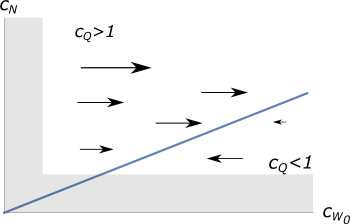
Figure 1: The parameter space of possible values of $c_{N}$ and $c_{W_{0}}$. In the grey area, one of these two control parameters is too small such that corrections are dangerously large. The blue line separates the regimes of validity of the two bounds in (3.12) and (3.14). The arrows specify how $c_{W_{0}}$ must change to decrease the lower bound $-Q_{3}^{*}(c_{N},c_{W_{0}})$ at fixed $c_{N}$.

Note that the subleading terms in (3.16) have a significant impact on the final bound one obtains. We only display the leading term to give the reader an intuition of how the bound scales with the parameters. However, to actually compute $N$ we always make use of the exact expression (3.11).

Thus, we require $Q_{3}$ to be negative and its absolute value to exceed the throat-flux $N$ since additional 3-form flux is needed to stabilize the complex-structure moduli. Let us discuss the implications of (3.16). The constraint specifies the minimal tadpole needed in LVS constructions to avoid the singular-bulk problem, and to make sure that the corrections induced by a varying warp factor and higher F-terms are parametrically suppressed. The degree of parametric suppression can be chosen at will by specifying $c_{N}$. The parameter $c_{N}$ determines to which extent warping effects are suppressed and fixes, through (3.15), the optimal value of $W_{0}$. The approximation of $x$ being close to zero improves with increasing $g_{s}M^{2}$ and increasing control parameters. Interestingly, the main expansion parameter $N_{\ast}$ coincides with the size of the small cycle $\tau_{s}$.

An optimistic bound on $N$ is obtained by using the metastability constraint $g_{s}M^{2}\gtrsim 12$ by KPV Kachru:2002gs (to be precise, $M>12$ combined with $g_{s}M\gtrsim 1$). Setting $\kappa_{s}=1$ and $a_{s}=\pi/3$ for the moment, as well as using (3.11) together with (3.15), we obtain for the minimal tadpole

$$N\simeq 33.6\qquad\text{for}\quad c_{N}=5\,\qquad\text{and}\,\qquad N\simeq 45.8\qquad\text{for}\quad c_{N}=100\,.$$ (3.17)

This is, however, probably too weak since it ignores backreaction. Indeed, the constraint comes from the process in which the $\overline{D3}$ polarises into a fluxed NS5, which slips over the equator of the $S^{3}$ at the tip of the throat. One expects that, as part of this decay process, the volume of the $S^{3}$ is driven to a smaller value, lowering the potential barrier for the decay.

An improvement has been suggested in Bena:2018fqc ; Blumenhagen:2019qcg (see also Douglas:2007tu ; Douglas:2008jx ), where the conifold modulus is treated as a dynamical variable. In Scalisi:2020jal this analysis was combined with the polarization of the $\overline{D3}$ into an NS5-brane. As already discussed in Gao:2020xqh ; Junghans:2022exo , the reliability of these analyses is limited by the assumption that the warp factor behaves as $\exp(4A(0))\sim|Z|^{4/3}$, also off-shell. This is not obvious because $\exp(4A(0))\sim\exp(-8\pi K/3g_{s}M)$ is a priori a fixed number, determined by the flux choice. Put differently, it is not clear why the warp factor should go to zero as the $S^{3}$ at the tip of the throat is dynamically driven to zero radius. After all, the fluxes $K$ and $M$ determining $\exp(4A(0))$ à la Klebanov-Strassler are discrete.

Nevertheless, we may take for the moment the value $g_{s}M^{2}\approx 46$ obtained in Bena:2018fqc ; Blumenhagen:2019qcg as a (probably rather conservative) lower bound and insert it together with (3.15) in (3.11). Choosing again $\kappa_{s}=1$ and $a_{s}=\pi/3$, we find

$$N\simeq 132.9\qquad\text{for}\quad c_{N}=5\qquad\text{and}\qquad N\simeq 179.9\qquad\text{for}\quad c_{N}=100\,.$$ (3.18)

Combined with the fact that, in the explicit LVS models considered to date the maximal tadpole is $\sim 150$ Crino:2020qwk , we see that the tadpole constraint is neither harmless nor deadly.

The natural way to ensure the constraint (3.16) is satisfied is to search for LVS compactifications with a large D3-tadpole. We will discuss the prospects for finding such examples and stabilizing all moduli in Sect. 4. In addition, one may try to study the LVS in more detail in the regime where the control parameters $c_{N}$ and $c_{W_{0}}$ are only moderately large. To convince oneself that the construction remains reliable, one would need to make sure that even higher order corrections of the same type do not blow up. Interestingly, (3.16) increases for small $\kappa_{s}$ and is independent of the Euler number. This appears to partly differ from the trend observed in example studies in Crino:2020qwk .

4 Discussion of the LVS Tadpole Constraint

4.1 Interplay with the Tadpole Problem

Our central result (3.16) provides a quantitative lower bound on the flux-induced D3 tadpole. The tadpole conjecture Bena:2020xrh ; Bena:2021wyr ; Plauschinn:2021hkp ; Lust:2021xds ; Bena:2021qty on the other hand states that, for a large number $h^{2,1}$ of complex structure (CS) moduli, the tadpole of the 3-form flux required to stabilize all of them in a non-singular regime grows faster than the negative tadpole of the corresponding orientifold geometry. If the conjecture were true, it would be logical to focus on LVS models with a large tadpole and a small number of moduli, escaping the allegedly dangerous asymptotic regime. But this may not be possible since, according to known examples, a large negative tadpole comes with a complicated topology (as discussed in more detail in Sect. 5 of Gao:2020xqh ) and hence many moduli. Indeed, one would expect that a single involution of a certain geometry has many O3 fixed points precisely because the topology is complicated. Similarly, while even a single O7 plane with its D7 branes can produce a large tadpole, this tadpole is tied to its topology. It grows if the 7-brane topology becomes complicated, which is in general associated with the presence of many brane-deformation moduli. These, in turn, require more flux to be stabilized.

It then seems that the allowed LVS vacua are constrained to an interval of permitted $Q_{3}$, with (3.16) providing a lower bound and the parametrics of the tadpole conjecture providing an upper bound above which it becomes hard to stabilize all the CS moduli. One might worry that further analyses will demonstrate that this interval shrinks to zero size, casting all LVS de Sitter vacua into the swampland. Indeed, this concern was already raised in Bena:2020xrh , though without deriving a quantitative LVS tadpole constraint. However, things need not be all doom and gloom:

We recall an important but perhaps underappreciated condition for the tadpole conjecture to apply, namely that the stabilized geometry is required to be smooth. For example, in the simple $K3\times K3$ example it is possible to stabilize all CS moduli (including D7 brane moduli in the language of F-theory) if singular geometries are permitted Dasgupta:1999ss ; Aspinwall:2005ad ; Braun:2008pz ; Braun:2014ola . According to the detailed study of Bena:2020xrh , developing the method of Braun:2008pz , this fails if one attempts to avoid the gauge enhancement through singularities. Nevertheless, this failure allows for the following more optimistic view on the possible string landscape of de Sitter vacua: The tadpole conjecture says that all vacua in the landscape at large number of CS moduli have singular internal geometries. One may embrace this statement together with the fact that the singularities will in general produce enhanced nonabelian gauge symmetries. The dynamics of those gauge theories together with SUSY breaking might stabilize the new moduli associated to the singularity. If this happens only at low energies, the nonabelian gauge theories make our compactification more interesting phenomenologically. The tadpole conjecture then tells us that the de Sitter vacua that do exist in the landscape are on average much more interesting phenomenologically then one a priori expects.

4.2 Overcoming the LVS Tadpole Constraint and further challenges

With these considerations in mind, let us look at which D3-tadpole has been achieved in IIB string theory and what the prospects for realizing higher tadpoles might be.

In IIB string theory, the $D3$ tadpole is generally given by

$$N_{D3}+\frac{N_{\text{flux}}}{2}+N_{\text{gauge}}=\frac{N_{O3}}{4}+\frac{\chi(D_{O7})}{12}+\sum_{a}N_{a}\,\frac{\chi(D_{a})+\chi(D^{\prime}_{a})}{48}\equiv-Q_{3}\,,$$ (4.1)

with $N_{\text{flux}}=\frac{1}{(2\pi)^{4}\alpha^{{}^{\prime}2}}\int H_{3}\wedge F_{3}$, $N_{\text{gauge}}=-\sum_{a}\frac{1}{8\pi^{2}}\int_{D_{a}}\text{tr}{\cal F}_{a}^{2}$, where ${\cal F}_{a}$ is the gauge flux turned on on each of the divisors $D_{a}$, and $N_{a}$ the number of D7 branes (their orientifold images) wrapping the divisor $D_{a}$ ($D^{\prime}_{a}$). Note that a throat with fluxes $K$ and $M$ contributes an amount of $2N=2KM$ to the quantity $N_{\rm flux}$ in (4.1). The reason is that a throat in the orientifold corresponds to two throats in the Calabi-Yau. If the D7 brane tadpole is cancelled locally by placing eight $D7$ branes on top of the $O7$ plane, (4.1) simplifies to

$$N_{D3}+\frac{N_{\text{flux}}}{2}+N_{\rm gauge}=\frac{N_{O3}}{4}+\frac{\chi(D_{O7})}{4}\,.$$ (4.2)

Most concrete type-IIB orientifolds considered in the literature are based on Calabi-Yaus with a small number of Kahler moduli $h^{1,1}(X)$. The highest negative tadpole values of explicitly considered models we are aware of are $Q_{3}=-149$ Crino:2020qwk and $-104$ Louis:2012nb , both in models with $h^{1,1}(X)=2$ and based on reflection involutions. More generally in type-IIB orientifolds with locally cancelled D7 tadpole, the negative contribution to the D3 tadpole can be bounded from above by the Lefschetz fixed point theorem Collinucci:2008pf ; Carta:2020ohw ; Bena:2020xrh :

$$-Q_{3}\leq 1+\frac{1}{2}\left(h^{1,1}+h^{2,1}\right)\,.$$ (4.3)

Using the largest Hodge numbers from the Kreuzer-Skarke dataset Kreuzer:2000xy , this gives, $-Q_{3}\leq 252$.

• Exploiting non-local D7-tadpole cancellation: In the models of Louis:2012nb ; Crino:2020qwk , the D7 tadpole is cancelled locally, i.e. eight D7 branes sit on top of each O7. This restricts the possibilities of getting a large tadpole: Indeed, according to Carta:2020ohw , canceling the D7 tadpole locally in smooth and favorable Complete Intersection Calabi-Yau three-folds (CICYs) with both reflections and simple divisor exchange involutions gives even tadpole values in the range $[-36,4]$. By contrast, non-local D7-tadpole cancellation produced values in the larger range $[-132,-12]$. Moreover, the study of toric orientifold Calabi-Yaus with $h^{1,1}\leq 6$ in Altman:2021pyc gave $Q_{3}\in[-30,0]$. This was based only on the divisor exchange involution and local D7-tadpole cancellation. Models with reflection involution in toric Calabi-Yaus are still under study but we expect that in this class the tadpole will increase significantly. The reason is that, in the examples of Louis:2012nb ; Crino:2020qwk with reflection involution the tadpole is already as large as $104$ and $149$ even for $h^{1,1}(X)=2$. Thus, one may hope that extending this to the range $h^{1,1}(X)\leq 6$ much larger tadpoles can arise.

• Using divisors $D_{a}$ with large Euler number : (a) From (4.1) one can see another reason for the limited tadpole range arising in the study of Carta:2020ohw . It is the fact that in CICYs the topology of each divisor is relatively simple and the largest Euler number of a divisor is modest: $\chi(D_{a})_{max}=80$ Carta:2020ohw ; Carta:2022oex . By contrast, in the toric setting even with $h^{1,1}(X)\leq 6$, the highest Euler number that gives an integer contribution to the tadpole is $\chi(D_{a})_{max}=504$ Altman:2021pyc . Even if we only consider a reflection on this divisor and cancel the D7-tadpole locally, it will contribute $-126$ to the tadpole. A distribution of Euler numbers of divisors in the orientifold Calabi-Yau database of Altman:2021pyc is displayed in Fig. 2.

  

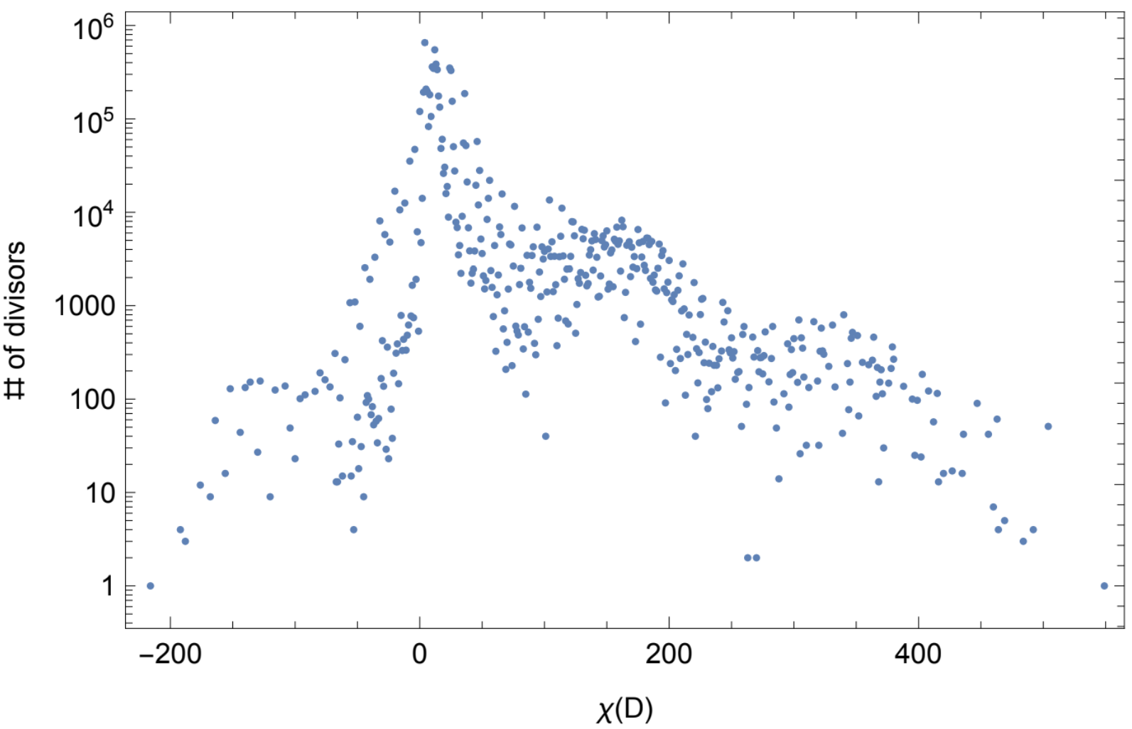
  Figure 2: Log distribution of the Euler number of individual divisors $\chi(D)$ in toric orientifold Calabi-Yaus with $h^{1,1}(X)\leq 6$.

   (b) Another way to enlarge the Euler number of $D_{a}$ is by considering a D7-brane wrapping a combination of divisors. This relies on detailed model building and represents an interesting project for the future.

• Large $h^{1,1}(X)$: Increasing $h^{1,1}(X)$ enriches the possibilities for D7-brane model building and hence should make it possible to find larger Euler number for $D_{a}$ and hence larger $N_{O3}$. For CICYs, the largest $h^{1,1}$ is just $19$ Candelas:1987kf while for toric Calabi-Yau this number increases to $h^{1,1}(X)=491$ Kreuzer:2000xy . Although so far no database for orientifolds of toric Calabi-Yaus with higher $h^{1,1}(X)$ exists, progress based on large cluster computation and machine learning has been made Gao:2021xbs . We note that in the search for large gauge groups, a correlation between the rank and $h^{1,1}$ has been observed Louis:2012nb . The concrete model studied in that paper has only $h^{1,1}=2$ and a maximal negative tadpole of $-92$, but the expectation is that models with much larger $h^{1,1}$ and D7 brane numbers going into the hundreds exist. While this raises the hope that very large negative tadpoles can also be achieved by the detailed study of the corresponding geometries, one in general pays the price of large $h^{1,1}$. This means many Kahler moduli, the stabilization of which may in itself be non-trivial in the LVS context, as we discuss below.

• Increasing $N_{O3}$: Finally, an obvious way forward is to search for models with more O3 planes. In the particularly tractable setting of CICYs, see e.g. Candelas:1987kf ; Anderson:2017aux , the multiplicities of O3 and O7 planes have recently been studied in Carta:2020ohw . Tadpoles in the range $[-132,-12]$ were found. An interesting aspect uncovered in this context is that the resolution branch of each conifold singularity on an O7 plane produces one extra O3. Although in Carta:2020ohw this did not lead to higher tadpoles, this might change in more general settings, such as toric Calabi-Yaus. Moreover, the existence of this method for increasing the number of O3 planes, possibly in the range of $N_{O3}\sim 100$, is interesting in itself.

If it should nevertheless prove impossible to construct perturbative type-IIB models with a sufficiently high tadpole to be in control according to (3.16) and with all CS-moduli stabilized in an acceptable manner, another option is to consider proper F-theory compactifications Vafa:1996xn ; Weigand:2010wm . The immediate advantage is that Calabi-Yau 4-folds with very large Euler number $\chi_{4}$ are known, leading to negative D3 tadpoles as high as $N=\chi_{4}/24=75852$ Klemm:1996ts ; Candelas:1997eh . This appears to be sufficient to easily satisfy the constraint (3.16) with excellent control. But the extension of the discussion to F-theory models has its price:

On the one hand, the key parametric relations $\ln{\cal V}\sim\tau_{s}\sim 1/g_{s}$ demand that we realise a small value of $g_{s}$ to achieve a large volume. In F-theory, $g_{s}$ is replaced by an appropriate average of the exponential of the dilaton, $g_{s}\equiv\langle e^{\phi}\rangle$. Studying whether a small $g_{s}$ can in this way be implemented in large-tadpole F-theory geometries is an interesting task.

On the other hand, a 4-fold with large Euler number implies, in the smooth case, that the F-theory model has either many Kahler moduli or many complex structure moduli or many 7-brane deformations (cf. Sect. 5 of Gao:2020xqh , based on Denef:2008wq ; Collinucci:2008pf ; Braun:2008ua ). The latter two options potentially run into trouble with the tadpole conjecture (though this may be acceptable if one allows for singular geometries). The former option, where the number of Kahler moduli is large, potentially has a problem with the LVS moduli stabilization procedure. Indeed, the standard approach to stabilizing non-blowup moduli (other than the volume) in the LVS is through loop corrections Cicoli:2007xp ; Cicoli:2008va . The dependence of such corrections on ratios of 4-cycle volumes as well as the complex-structure moduli dependence of the prefactors is not known except for simple torus orbifold geometries Berg:2005ja ; Berg:2007wt (see Gao:2022uop for an attempt to make progress). This may not be a problem as a matter of principle since, generically, one expects that all Kahler moduli will somehow be stabilized by loop effects. But clearly it is a problem if one wants to establish rigorously the existence of at least one explicit LVS de Sitter model. Hence, the way forward may be not to rely on loops but rather demand that all ratios of non-blowup cycles are stabilized by $D$-term constraints Jockers:2005zy ; Haack:2006cy ; Blumenhagen:2007sm . In this case, achieving a purely algebraic and fully explicit construction in the near future appears more plausible.

The correction we have focused on in this note is not the only correction relevant for control in the LVS. As emphasized in Junghans:2022exo , further potentially dangerous corrections are associated with logarithmic terms. There are two types:

One of them Conlon:2010ji derives from the field redefinition $\tau^{\prime}_{s}\equiv\tau_{s}+\alpha\log(\mathcal{V})$, where $\tau_{s}^{\prime}$ rather than $\tau_{s}$ is now the real part of the proper Kahler variable. The Kahler potential then reads

$$K\sim-2\log\left[\tau_{b}^{3/2}-\left(\tau_{s}^{\prime}-\alpha\log\left(\mathcal{V}\right)\right)^{3/2}+..\right]+..\,,$$ (4.4)

with the physical small-cycle volume being $(\tau_{s}^{\prime}-\alpha\log(\mathcal{V}))$. It is at the moment not entirely settled if and when such a correction appears in string compactifications. A surprising aspect is the implicit claim that, at ${\cal V}\to\infty$, the correction grows in importance. For example, the size of non-perturbative effects $\sim\exp(-a_{s}\tau_{s}^{\prime})$ now has a very different relation to the physical volumes of small cycle and Calabi-Yau.

Another type of correction, corresponding to a replacement $\mathcal{V}\to\mathcal{V}+\alpha\log(\mathcal{V})$, has been proposed to appear through the interplay of the $R^{4}_{10}$ and D7/O7 branes Antoniadis:2019rkh . An interesting aspect of this proposal is that, while it indeed threatens parametric control of the LVS, it could instead allow for alternative ways to realize a de Sitter minimum.

The correction (3.8) we have focused on in this note and log corrections are not the only potentially relevant corrections for the LVS. As recently highlighted in Junghans:2022exo , a host of further corrections are interesting or even potentially dangerous. This requires more research. In this context, in Gao:2022uop , we give a general discussion of loop corrections to the Kahler moduli Kahler potential. While important in many ways, we do not see that these corrections endanger the basic setting of the LVS.

Finally, we emphasize again that the tadpole constraint (3.16) is tied to the $\overline{\rm D3}$-uplift. Hence, even if this constraint turned out to remain problematic for the LVS, other uplifting mechanisms could work more successfully, especially if they do not require a very large tadpole. One example is the $D$-term uplift, where the positive energy arises because a D7-brane matter-field is unable to satisfy simultaneously a $D$-term and an $F$-term constraint Achucarro:2006zf ; Cremades:2007ig . Implementing this consistently in the stringy geometry leads to the concept of a T-brane uplift Cicoli:2015ylx . Another suggestion is the Winding uplift Hebecker:2020ejb ; Carta:2021sms (with the idea going back to Hebecker:2015rya ), which uses the possibility to create a perturbatively flat direction in the complex-structure moduli space by an appropriate flux choice Hebecker:2015rya . The non-perturbatively small potential along this flat valley can then arguably be tuned such that a local metastable minimum with non-zero $F$-term arises. In this setting, the tuning power of the complex-structure landscape could help to realize an exponentially small uplift without a warped throat.

5 Summary

The core result of this short note is (3.16), which bounds the D3 tadpole required in LVS models from below. The bound comes from demanding that warping corrections in the bulk, associated with the Klebanov-Strassler throat housing the anti-D3 brane uplift, are under control. While this constrains the set of geometries suitable for an LVS with a controlled uplift, we so far see no catastrophe that places all LVS vacua in the swampland. Rather, the bound poses a challenge for LVS model-building which one can attempt to overcome by searching for compactifications with a sufficiently large D3-tadpole. While the tadpole conjecture poses an additional challenge in this context, we do not currently see this as impossible to overcome. In type-IIB a tadpole of 149 has been achieved Crino:2020qwk , but, as we argued above, much larger tadpoles may be possible. In F-theory, the largest available tadpole of $75852$ Klemm:1996ts ; Candelas:1997eh easily satisfies our bound (3.16) with excellent control. However, then one faces other challenges: One either has to realize a small averaged $g_{s}$ in F-theory or, alternatively, one has to replace the control parameter $1/g_{s}$ by a topology which makes the coefficient of the $\alpha^{\prime 3}$ correction appropriately large. Moreover, stabilizing all moduli in a controlled manner in geometrically complicated models with high tadpole may introduce new difficulties. Finally, a key quantity determining the bound of the D3 tadpole (3.16) is $g_{s}M^{2}$, the minimal value of which is still under debate. In order to see how constraining the bound for the LVS really is, it would be essential to know this value as precisely as possible.

We hope that this note has highlighted a number of directions for future work which can help to clarify whether LVS de Sitter vacua exist.

Appendix A Derivation of the $\overline{D3}$ Uplift Potential

In this appendix we derive the uplift potential directly from the Klebanov-Strassler (KS) geometry Klebanov:2000hb , using also Klebanov:2000nc ; Herzog:2001xk . This provides a more precise derivation of the (non-backreacted) uplift potential than we are aware of elsewhere in the literature.

The warp factor in string frame far away from the tip of the throat is given by the following two equivalent expressions. Firstly, it can be parametrized by the flux $N=KM$ and the radial distance from the tip $r=r_{\text{max}}$ at which the total flux in the throat equals $N$. At $r_{\text{max}}$, the throat is glued into the compact Calabi-Yau. This yields Klebanov:2000nc ; Herzog:2001xk

$$h_{N}(r)=\frac{27\pi\alpha^{\prime 2}}{4r^{4}}\left(g_{s}N+\frac{3(g_{s}M)^{2}}{2\pi}\ln(r/r_{\text{max}})+\frac{3}{8\pi}(g_{s}M)^{2}\right)\,.$$ (A.1)

Secondly, we may use the KS warp factor $h_{\varepsilon}^{\text{KS}}(r)$ which describes both the UV and the smooth, IR region and which is parametrized by the conifold resolution parameter $\varepsilon$ Klebanov:2000hb ; Herzog:2001xk . In the UV, it has the approximate form

$$h_{\varepsilon}^{\text{KS}}(r)\simeq\frac{81(\alpha^{\prime}g_{s}M)^{2}}{8r^{4}}\ln\left(\left(\frac{2^{5/3}}{3}\right)^{1/2}\frac{r}{\varepsilon^{2/3}}\right)\,.$$ (A.2)

Comparing (A.1) and (A.2) determines $r_{\text{max}}$ as a function of $\varepsilon$ to leading order to be

$$r_{\text{max}}=\left(\frac{3}{2^{5/3}}\right)^{1/2}\varepsilon^{2/3}\,\text{e}^{\frac{2\pi K}{3g_{s}M}}\,.$$ (A.3)

Moreover, from KS, the warp factor at the tip is known. In string frame, it reads

$$h_{\varepsilon}^{\text{KS}}(0)=\frac{2^{2/3}a_{0}(g_{s}M\alpha^{\prime})^{2}}{\varepsilon^{8/3}}\,,$$ (A.4)

with the constant $a_{0}\approx 0.71805$.

With this in hand, we can calculate the ratio of the warp factors at the tip and far away from the tip at $r=r_{\text{max}}$. This yields the relative warping needed for the uplift potential:

$$\frac{h_{\varepsilon}^{\text{KS}}(0)}{h_{\varepsilon}^{\text{KS}}(r=r_{\text{max}})}=\frac{a_{0}}{3\,2^{2/3}\pi}\,\frac{g_{s}M^{2}}{N}\text{e}^{\frac{8\pi K}{3g_{s}M}}\,.$$ (A.5)

So far, we neglected the additive, constant contribution $\sim\mathcal{V}^{2/3}$ to the warp factor Giddings:2005ff which becomes dominant at sufficiently large volume. Specifically, we replace the KS warp factor according to

$$h_{\epsilon}^{\rm KS}(r)\qquad\to\qquad({\cal V}_{s}/{\cal V}_{s,0})^{2/3}\,h_{\epsilon}^{\rm KS}(r_{\rm max})\,+\,h_{\epsilon}^{\rm KS}(r)\,.$$ (A.6)

Here we normalized the constant term by introducing a string-frame, fiducial volume ${\cal V}_{s,0}$. Our definition implies that, if ${\cal V}_{s}={\cal V}_{s,0}$, the strong-warping region is set by $r\lesssim r_{\rm max}$. This is the situation when a strongly warped throat is glued into a weakly warped, compact CY. For larger ${\cal V}_{s}$, a weakly-warped conical region develops above the throat (see e.g. Brummer:2005sh ). From all of this, it should be clear that ${\cal V}_{s,0}$ must be chosen such that typical length scales in the CY match typical length scales of the $T^{1,1}$ at $r_{\rm max}$. Hence, for ${\cal V}_{s}\gg{\cal V}_{s,0}$, the full, inverse warp factor at the tip is given by

$$\text{e}^{4A(0)}=\left(\frac{\mathcal{V}_{s}}{\mathcal{V}_{s,0}}\right)^{2/3}\frac{h_{\varepsilon}^{\text{KS}}(r=r_{\text{max}})}{h_{\varepsilon}^{\text{KS}}(0)}\,=\left(\frac{\mathcal{V}_{s}}{(\left.\text{Vol}(T^{1,1})\right|_{r_{\text{max}}})^{6/5}}\right)^{2/3}\frac{h_{\varepsilon}^{\text{KS}}(r=r_{\text{max}})}{h_{\varepsilon}^{\text{KS}}(0)}\,.$$ (A.7)

The volume scaling of this expression matches the corrected volume scaling of Kachru:2003sx .

To obtain the final formula of the uplift potential, we hence need to determine the volume of the $T^{1,1}$ at $r_{\text{max}}$. For this we consider the string frame metric of the conifold far away from the tip

$$\mathrm{d}s_{10}^{2}=h_{N}^{-1/2}(r)\,\eta_{\mu\nu}\mathrm{d}x^{\mu}\mathrm{d}x^{\nu}+h_{N}^{1/2}(r)\left(\mathrm{d}r^{2}+r^{2}\mathrm{d}s_{T^{1,1}}^{2}\right)\,.$$ (A.8)

Using (A.1) and Vol$\,T^{1,1}=16\pi^{3}/27$ from Gubser:1998vd , we find

$$\mathcal{V}_{s,0}^{2/3}=\frac{3^{3/5}}{2^{14/5}\,\pi^{3/5}}\left(g_{s}N+\frac{3}{8\pi}(g_{s}M)^{2}\right)\,.$$ (A.9)

This can be plugged into (A.7) which then yields the uplift potential

$$V_{\text{uplift}}=V_{\overline{D3}}=2T_{D3}e^{4A(0)}=\frac{\left(3^{2}\,\pi^{3}\,2^{22/3}\right)^{1/5}}{a_{0}}\,\frac{\text{e}^{-\frac{8\pi K}{3g_{s}M}}}{g_{s}M^{2}\mathcal{V}^{4/3}}\,.$$ (A.10)

Here we only used the leading, first term on the r.h. side of (A.9). Note that the $g_{s}M^{2}$ dependence of our the uplift potential agrees with the results of the supergravity-based approach of Douglas:2007tu ; Douglas:2008jx ; Bena:2018fqc . At the moment, we do not understand why this agreement occurs in spite of the absence of a fiducial volume ${\cal V}_{s,0}$ in these references. In our approach, ${\cal V}_{s,0}$ contributes essentially to the final result.

References

- (1) S. Kachru, R. Kallosh, A.D. Linde and S.P. Trivedi, De Sitter vacua in string theory, Phys. Rev. D 68 (2003) 046005 [hep-th/0301240].
- (2) V. Balasubramanian, P. Berglund, J.P. Conlon and F. Quevedo, Systematics of moduli stabilisation in Calabi-Yau flux compactifications, JHEP 03 (2005) 007 [hep-th/0502058].
- (3) U.H. Danielsson and T. Van Riet, What if string theory has no de Sitter vacua?, Int. J. Mod. Phys. D 27 (2018) 1830007 [1804.01120].
- (4) G. Obied, H. Ooguri, L. Spodyneiko and C. Vafa, De Sitter Space and the Swampland, 1806.08362.
- (5) S.K. Garg and C. Krishnan, Bounds on Slow Roll and the de Sitter Swampland, JHEP 11 (2019) 075 [1807.05193].
- (6) H. Ooguri, E. Palti, G. Shiu and C. Vafa, Distance and de Sitter Conjectures on the Swampland, Phys. Lett. B 788 (2019) 180 [1810.05506].
- (7) I. Bena, M. Grana and N. Halmagyi, On the Existence of Meta-stable Vacua in Klebanov-Strassler, JHEP 09 (2010) 087 [0912.3519].
- (8) I. Bena, G. Giecold, M. Grana, N. Halmagyi and S. Massai, The backreaction of anti-D3 branes on the Klebanov-Strassler geometry, JHEP 06 (2013) 060 [1106.6165].
- (9) B. Michel, E. Mintun, J. Polchinski, A. Puhm and P. Saad, Remarks on brane and antibrane dynamics, JHEP 09 (2015) 021 [1412.5702].
- (10) J. Blåbäck, F.F. Gautason, A. Ruipérez and T. Van Riet, Anti-brane singularities as red herrings, JHEP 12 (2019) 125 [1907.05295].
- (11) J. Moritz, A. Retolaza and A. Westphal, Toward de Sitter space from ten dimensions, Phys. Rev. D 97 (2018) 046010 [1707.08678].
- (12) F. Carta, J. Moritz and A. Westphal, Gaugino condensation and small uplifts in KKLT, JHEP 08 (2019) 141 [1902.01412].
- (13) F.F. Gautason, V. Van Hemelryck, T. Van Riet and G. Venken, A 10d view on the KKLT AdS vacuum and uplifting, JHEP 06 (2020) 074 [1902.01415].
- (14) Y. Hamada, A. Hebecker, G. Shiu and P. Soler, Understanding KKLT from a 10d perspective, JHEP 06 (2019) 019 [1902.01410].
- (15) S. Kachru, M. Kim, L. Mcallister and M. Zimet, de Sitter vacua from ten dimensions, JHEP 12 (2021) 111 [1908.04788].
- (16) Y. Hamada, A. Hebecker, G. Shiu and P. Soler, Completing the D7-brane local gaugino action, JHEP 11 (2021) 033 [2105.11467].
- (17) X. Gao, A. Hebecker and D. Junghans, Control issues of KKLT, Fortsch. Phys. 68 (2020) 2000089 [2009.03914].
- (18) F. Carta and J. Moritz, Resolving spacetime singularities in flux compactifications & KKLT, JHEP 08 (2021) 093 [2101.05281].
- (19) M. Demirtas, M. Kim, L. McAllister, J. Moritz and A. Rios-Tascon, Small cosmological constants in string theory, JHEP 12 (2021) 136 [2107.09064].
- (20) D. Junghans, LVS de Sitter Vacua are probably in the Swampland, 2201.03572.
- (21) I. Bena, J. Blåbäck, M. Graña and S. Lüst, The Tadpole Problem, 2010.10519.
- (22) C. Crinò, F. Quevedo and R. Valandro, On de Sitter String Vacua from Anti-D3-Branes in the Large Volume Scenario, JHEP 03 (2021) 258 [2010.15903].
- (23) S.P. de Alwis, On integrating out heavy fields in SUSY theories, Phys. Lett. B 628 (2005) 183 [hep-th/0506267].
- (24) M. Cicoli, J.P. Conlon, A. Maharana and F. Quevedo, A Note on the Magnitude of the Flux Superpotential, JHEP 01 (2014) 027 [1310.6694].
- (25) D. Ciupke, J. Louis and A. Westphal, Higher-Derivative Supergravity and Moduli Stabilization, JHEP 10 (2015) 094 [1505.03092].
- (26) J.P. Conlon and F.G. Pedro, Moduli Redefinitions and Moduli Stabilisation, JHEP 06 (2010) 082 [1003.0388].
- (27) I. Antoniadis, Y. Chen and G.K. Leontaris, Logarithmic loop corrections, moduli stabilisation and de Sitter vacua in string theory, JHEP 01 (2020) 149 [1909.10525].
- (28) J.P. Conlon and E. Palti, Gauge Threshold Corrections for Local Orientifolds, JHEP 09 (2009) 019 [0906.1920].
- (29) M. Weissenbacher, F-theory vacua and -corrections, JHEP 04 (2020) 032 [1901.04758].
- (30) T.W. Grimm, J. Keitel, R. Savelli and M. Weissenbacher, From M-theory higher curvature terms to corrections in F-theory, Nucl. Phys. B 903 (2016) 325 [1312.1376].
- (31) T.W. Grimm, T.G. Pugh and M. Weissenbacher, The effective action of warped M-theory reductions with higher-derivative terms - Part II, JHEP 12 (2015) 117 [1507.00343].
- (32) D. Junghans and G. Shiu, Brane curvature corrections to the 1 type II/F-theory effective action, JHEP 03 (2015) 107 [1407.0019].
- (33) G. von Gersdorff and A. Hebecker, Kahler corrections for the volume modulus of flux compactifications, Phys. Lett. B 624 (2005) 270 [hep-th/0507131].
- (34) M. Berg, M. Haack and B. Kors, String loop corrections to Kahler potentials in orientifolds, JHEP 11 (2005) 030 [hep-th/0508043].
- (35) M. Berg, M. Haack and E. Pajer, Jumping Through Loops: On Soft Terms from Large Volume Compactifications, JHEP 09 (2007) 031 [0704.0737].
- (36) M. Cicoli, J.P. Conlon and F. Quevedo, Systematics of String Loop Corrections in Type IIB Calabi-Yau Flux Compactifications, JHEP 01 (2008) 052 [0708.1873].
- (37) M. Cicoli, J.P. Conlon and F. Quevedo, General Analysis of LARGE Volume Scenarios with String Loop Moduli Stabilisation, JHEP 10 (2008) 105 [0805.1029].
- (38) C.P. Burgess, M. Cicoli, D. Ciupke, S. Krippendorf and F. Quevedo, UV Shadows in EFTs: Accidental Symmetries, Robustness and No-Scale Supergravity, Fortsch. Phys. 68 (2020) 2000076 [2006.06694].
- (39) M. Cicoli, F. Quevedo, R. Savelli, A. Schachner and R. Valandro, Systematics of the ’ expansion in F-theory, JHEP 08 (2021) 099 [2106.04592].
- (40) R. Minasian, T.G. Pugh and R. Savelli, F-theory at order , JHEP 10 (2015) 050 [1506.06756].
- (41) X. Gao, A. Hebecker, S. Schreyer and G. Venken, Loops, Local Corrections and Warping in the LVS and other Type IIB Models, 2204.06009.
- (42) I. Bena, J. Blåbäck, M. Graña and S. Lüst, Algorithmically solving the Tadpole Problem, 2103.03250.
- (43) E. Plauschinn, The tadpole conjecture at large complex-structure, 2109.00029.
- (44) S. Lüst, Large complex structure flux vacua of IIB and the Tadpole Conjecture, 2109.05033.
- (45) I. Bena, C. Brodie and M. Graña, D7 Moduli Stabilization: The Tadpole Menace, 2112.00013.
- (46) K. Becker, M. Becker, M. Haack and J. Louis, Supersymmetry breaking and alpha-prime corrections to flux induced potentials, JHEP 06 (2002) 060 [hep-th/0204254].
- (47) A. Hebecker, S.C. Kraus, M. Kuntzler, D. Lust and T. Weigand, Fluxbranes: Moduli Stabilisation and Inflation, JHEP 01 (2013) 095 [1207.2766].
- (48) I. Bena, E. Dudas, M. Graña and S. Lüst, Uplifting Runaways, Fortsch. Phys. 67 (2019) 1800100 [1809.06861].
- (49) R. Blumenhagen, D. Kläwer and L. Schlechter, Swampland Variations on a Theme by KKLT, JHEP 05 (2019) 152 [1902.07724].
- (50) S. Kachru, R. Kallosh, A.D. Linde, J.M. Maldacena, L.P. McAllister and S.P. Trivedi, Towards inflation in string theory, JCAP 10 (2003) 013 [hep-th/0308055].
- (51) I.R. Klebanov and M.J. Strassler, Supergravity and a confining gauge theory: Duality cascades and chi SB resolution of naked singularities, JHEP 08 (2000) 052 [hep-th/0007191].
- (52) J.P. Conlon, F. Quevedo and K. Suruliz, Large-volume flux compactifications: Moduli spectrum and D3/D7 soft supersymmetry breaking, JHEP 08 (2005) 007 [hep-th/0505076].
- (53) M. Cicoli, F. Muia and P. Shukla, Global Embedding of Fibre Inflation Models, JHEP 11 (2016) 182 [1611.04612].
- (54) M. Cicoli, D. Ciupke, V.A. Diaz, V. Guidetti, F. Muia and P. Shukla, Chiral Global Embedding of Fibre Inflation Models, JHEP 11 (2017) 207 [1709.01518].
- (55) I. Antoniadis, S. Ferrara, R. Minasian and K.S. Narain, R**4 couplings in M and type II theories on Calabi-Yau spaces, Nucl. Phys. B 507 (1997) 571 [hep-th/9707013].
- (56) F. Denef and M.R. Douglas, Distributions of flux vacua, JHEP 05 (2004) 072 [hep-th/0404116].
- (57) S. Kachru, J. Pearson and H.L. Verlinde, Brane / flux annihilation and the string dual of a nonsupersymmetric field theory, JHEP 06 (2002) 021 [hep-th/0112197].
- (58) M. Scalisi, P. Soler, V. Van Hemelryck and T. Van Riet, Conifold dynamics and axion monodromies, JHEP 10 (2020) 133 [2007.15391].
- (59) M.R. Douglas, J. Shelton and G. Torroba, Warping and supersymmetry breaking, 0704.4001.
- (60) M.R. Douglas and G. Torroba, Kinetic terms in warped compactifications, JHEP 05 (2009) 013 [0805.3700].
- (61) K. Dasgupta, G. Rajesh and S. Sethi, M theory, orientifolds and G - flux, JHEP 08 (1999) 023 [hep-th/9908088].
- (62) P.S. Aspinwall and R. Kallosh, Fixing all moduli for M-theory on K3xK3, JHEP 10 (2005) 001 [hep-th/0506014].
- (63) A.P. Braun, A. Hebecker, C. Ludeling and R. Valandro, Fixing D7 Brane Positions by F-Theory Fluxes, Nucl. Phys. B 815 (2009) 256 [0811.2416].
- (64) A.P. Braun, Y. Kimura and T. Watari, The Noether-Lefschetz problem and gauge-group-resolved landscapes: F-theory on K3 K3 as a test case, JHEP 04 (2014) 050 [1401.5908].
- (65) J. Louis, M. Rummel, R. Valandro and A. Westphal, Building an explicit de Sitter, JHEP 10 (2012) 163 [1208.3208].
- (66) A. Collinucci, F. Denef and M. Esole, D-brane Deconstructions in IIB Orientifolds, JHEP 02 (2009) 005 [0805.1573].
- (67) F. Carta, J. Moritz and A. Westphal, A landscape of orientifold vacua, JHEP 05 (2020) 107 [2003.04902].
- (68) M. Kreuzer and H. Skarke, Complete classification of reflexive polyhedra in four-dimensions, Adv. Theor. Math. Phys. 4 (2000) 1209 [hep-th/0002240].
- (69) R. Altman, J. Carifio, X. Gao and B. Nelson, Orientifold Calabi-Yau Threefolds with Divisor Involutions and String Landscape, 2111.03078.
- (70) F. Carta, A. Mininno and P. Shukla, Systematics of perturbatively flat flux vacua for CICYs, 2201.10581.
- (71) P. Candelas, A.M. Dale, C.A. Lutken and R. Schimmrigk, Complete Intersection Calabi-Yau Manifolds, Nucl. Phys. B 298 (1988) 493.
- (72) X. Gao and H. Zou, Machine Learning to the Orientifold Calabi-Yau with String Vacua, 2112.04950.
- (73) L.B. Anderson, X. Gao, J. Gray and S.-J. Lee, Fibrations in CICY Threefolds, JHEP 10 (2017) 077 [1708.07907].
- (74) C. Vafa, Evidence for F theory, Nucl. Phys. B 469 (1996) 403 [hep-th/9602022].
- (75) T. Weigand, Lectures on F-theory compactifications and model building, Class. Quant. Grav. 27 (2010) 214004 [1009.3497].
- (76) A. Klemm, B. Lian, S.S. Roan and S.-T. Yau, Calabi-Yau fourfolds for M theory and F theory compactifications, Nucl. Phys. B 518 (1998) 515 [hep-th/9701023].
- (77) P. Candelas, E. Perevalov and G. Rajesh, Toric geometry and enhanced gauge symmetry of F theory / heterotic vacua, Nucl. Phys. B 507 (1997) 445 [hep-th/9704097].
- (78) F. Denef, Les Houches Lectures on Constructing String Vacua, Les Houches 87 (2008) 483 [0803.1194].
- (79) A.P. Braun, A. Hebecker and H. Triendl, D7-Brane Motion from M-Theory Cycles and Obstructions in the Weak Coupling Limit, Nucl. Phys. B 800 (2008) 298 [0801.2163].
- (80) H. Jockers and J. Louis, D-terms and F-terms from D7-brane fluxes, Nucl. Phys. B 718 (2005) 203 [hep-th/0502059].
- (81) M. Haack, D. Krefl, D. Lust, A. Van Proeyen and M. Zagermann, Gaugino Condensates and D-terms from D7-branes, JHEP 01 (2007) 078 [hep-th/0609211].
- (82) R. Blumenhagen, S. Moster and E. Plauschinn, Moduli Stabilisation versus Chirality for MSSM like Type IIB Orientifolds, JHEP 01 (2008) 058 [0711.3389].
- (83) A. Achucarro, B. de Carlos, J.A. Casas and L. Doplicher, De Sitter vacua from uplifting D-terms in effective supergravities from realistic strings, JHEP 06 (2006) 014 [hep-th/0601190].
- (84) D. Cremades, M.P. Garcia del Moral, F. Quevedo and K. Suruliz, Moduli stabilisation and de Sitter string vacua from magnetised D7 branes, JHEP 05 (2007) 100 [hep-th/0701154].
- (85) M. Cicoli, F. Quevedo and R. Valandro, De Sitter from T-branes, JHEP 03 (2016) 141 [1512.04558].
- (86) A. Hebecker and S. Leonhardt, Winding Uplifts and the Challenges of Weak and Strong SUSY Breaking in AdS, JHEP 03 (2021) 284 [2012.00010].
- (87) F. Carta, A. Mininno, N. Righi and A. Westphal, Gopakumar-Vafa hierarchies in winding inflation and uplifts, JHEP 05 (2021) 271 [2101.07272].
- (88) A. Hebecker, P. Mangat, F. Rompineve and L.T. Witkowski, Winding out of the Swamp: Evading the Weak Gravity Conjecture with F-term Winding Inflation?, Phys. Lett. B 748 (2015) 455 [1503.07912].
- (89) I.R. Klebanov and A.A. Tseytlin, Gravity duals of supersymmetric SU(N) x SU(N+M) gauge theories, Nucl. Phys. B 578 (2000) 123 [hep-th/0002159].
- (90) C.P. Herzog, I.R. Klebanov and P. Ouyang, Remarks on the warped deformed conifold, in Modern Trends in String Theory: 2nd Lisbon School on g Theory Superstrings, 8, 2001 [hep-th/0108101].
- (91) S.B. Giddings and A. Maharana, Dynamics of warped compactifications and the shape of the warped landscape, Phys. Rev. D 73 (2006) 126003 [hep-th/0507158].
- (92) F. Brummer, A. Hebecker and E. Trincherini, The Throat as a Randall-Sundrum model with Goldberger-Wise stabilization, Nucl. Phys. B 738 (2006) 283 [hep-th/0510113].
- (93) S.S. Gubser, Einstein manifolds and conformal field theories, Phys. Rev. D 59 (1999) 025006 [hep-th/9807164].