A Neural Phillips Curve and a Deep Output Gap

Abstract

Many problems plague the estimation of Phillips curves. Among them is the hurdle that the two key components, inflation expectations and the output gap, are both unobserved. Traditional remedies include creating reasonable proxies for the notable absentees or extracting them via some form of assumptions-heavy filtering procedure. I propose an alternative route: a Hemisphere Neural Network (HNN) whose peculiar architecture yields a final layer where components can be interpreted as latent states within a Neural Phillips Curve. There are benefits. First, HNN conducts the supervised estimation of nonlinearities that arise when translating a high-dimensional set of observed regressors into latent states. Second, computations are fast. Third, forecasts are economically interpretable. Fourth, inflation volatility can also be predicted by merely adding a hemisphere to the model. Among other findings, the contribution of real activity to inflation appears severely underestimated in traditional econometric specifications. Also, HNN captures out-of-sample the 2021 upswing in inflation and attributes it first to an abrupt and sizable disanchoring of the expectations component, followed by a wildly positive gap starting from late 2020. HNN’s gap unique path comes from dispensing with unemployment and GDP in favor of an amalgam of nonlinearly processed alternative tightness indicators – some of which are skyrocketing as of early 2022.

1 Introduction

Few equations are as central to modern macroeconomics and current monetary policy debates as the Phillips Curve (PC) – and its modern incarnation, the New Keynesian Phillips Curve (NKPC). Yet, many problems plague its estimation and thus, our understanding of how increasing economic activity translates into higher pressures on the price level. Similarly, our understanding of how inflation expectations influence current inflation is also compromised.

This paper focuses on a predictive Phillips curve – building an equation that uses, among other things, some measure of real activity to forecast inflation. It provides a new solution to an extremely pervasive problem in empirical inflation modeling and economics research in general. Namely, the two key components of the NKPC, inflation expectations ($\mathcal{E}_{t}$) and the output gap ($g_{t}$), are both unobserved. Instantly, this opens the gates to the proxies’ zoo. Which gap to choose? Which inflation expectations at what horizon from whom? Those are crucial empirical choices on which theory is practically silent. $\mathcal{E}_{t}$ and $g_{t}$ are necessary to produce and understand inflation forecasts, both of which are needed to guide monetary policy action – especially entering 2022.

A Hemisphere Neural Network. Taking a step back, what basic macroeconomic theory tells us, is that two sufficient statistics summarizing different groups of economic indicators should predict inflation reasonably well. More precisely, we know that (i) there should exist some abstract output gap, or in other words, a possibly nonlinear combination of variables related to the state of the economy (labor markets, industrial production, national accounts) that influence inflation, and (ii) some combination of price variables (past CPI values and several others) and other measures of inflation expectations also impact inflation directly. I make this vision operational by developing a new Deep Neural Network (DNN) architecture coined Hemisphere Neural Network (HNN). As the name suggests, the DNN is restricted so that its final inflation prediction is the sum of components composed from groups of predictors separated at the entrance of the network into different hemispheres. The peculiar structure allows the interpretation of the final layer’s cells output as key macroeconomic latent states in a linear equation – the NKPC. Moreover, the estimation of time-varying PC coefficients and the key latent states is performed within a single model.

While HNN’s development is motivated from inflation, its applicability extends to the various problems in economics where the link between "theoretical variables" and "Excel variables" is not crystal clear. Examples include the neutral interest rate, Taylor rules inputs, term premium, and of great interest recently, "financial conditions" in adrian2019’s quantile regressions of GDP growth – a non-trivial and non-innocuous modeling choice (plagborg2020growth). This extends to poorly measured observed explanatory variables. Thus, econometrically, this paper develops a new tool, rooted in modern deep learning machinery, to take the mismeasurement error bull by the horns. Obviously, HNN is by no means the first methodology dealing with latent state extraction (harvey1990forecasting; durbin2012time) or attenuation bias (schennach2016recent). But, when compared to the older generation of methods, its empirical merits will be decisive.

This paper sits at the intersection of at least four literatures: estimating the output gap, estimating Phillips curves, interpretable artificial intelligence, and the application of deep learning methods in macroeconomic forecasting. Given how vast those literatures are, the substantial review and discussion of them are relegated to its own Section 3. By blending them into a common goal, substantial amelioration over traditional methods are attainable. In short, the method has four key advantages. First, by the virtues of being a supervised learning problem, HNN improves over methods where $g_{t}$ is extracted from an economic activity series and then thrown in a "second stage" PC regression. That is, ${g}_{t}^{\text{HNN}}$ is by construction the most relevant summary statistic of real activity to explain inflation.

Second, with respect to econometric methods that included some mild form of supervision in the estimation of $g_{t}$ (kichian1999measuring; blanchard2015inflation; chan2016; chan2018; hasenzagl2018model; jarocinski2018inflation), HNN improves by dropping restrictive law of motion assumptions inherent to a state-space methodology. It also handles easily a high-dimensional group of inputs for both $g_{t}$ and $\mathcal{E}_{t}$ and carries computations quickly through standard highly optimized deep learning software.

Third, nonlinearities in how activity variables translate into $g_{t}$ or $\mathcal{E}_{t}$ (and ultimately $\pi_{t}$) are allowed through a deep and wide network architecture with over 2 million parameters. This is, in fact, a necessary feature given the accumulating evidence that the PC might be nonlinear with respect to traditional slack indicators (linde2019resolving; MRF; forbes2021low). Fourth, with respect to the numerous applications of neural networks in macroeconomic forecasting (see references in Section 3), HNN improves by being interpretable – through the components of the neural PC. Moreover, unlike most econometric applications of NNs, HNN fully embrace the implications from double descent phenomenon (belkin2019reconciling; hastie2019surprises; bartlett2020benign) by being overtly overparametrized and yet providing stellar results.

Results. Two main variants of HNN are proposed. The first one (HNN) is less restrictive on how exogenous time-variation mixes with other nonlinearities. The caveat is that only the gap’s contribution to inflation can be extracted from such a model. The second architecture (HNN-F, the flagship model) has a built-in factorization which allows to disentangle $g_{t}$’s estimates from its exogenously time-varying coefficient.

Many new insights are obtained. First, forecasts are typically much better than traditional PC-based forecasts. Unlike plain DNNs, this can be understood in economic terms. For the post-2008 period, this can be partly attributed to HNN-F’s gap – projected out-of-sample – closing much faster than traditional ones, then slips back gently into negative territory in the mid-2010s. HNN also captures the 2021 upswing in inflation and attributes it first to a rapid disanchoring in the expectations component, and then to a strongly positive output gap. While both effects’ peak are comparable in size to the 1970s, the components show much less persistence than they did four decades ago—in line with the stop-and-go nature of economic constraints of the Pandemic era. Second, throughout the whole sample and for both architectures, the contribution of the output gap component is shown to be much higher than what is reported from time-varying PC regression with traditional gap measures. Thus, it appears that mismeasuring $g_{t}$, to no astounding surprise, can severely bias downward its estimated impact on the price level. Conversely, the effect of the expectations component is found to be milder overall, with the notable exception of 2021, where it radically jumps upward while traditional estimates remain flat. Third, the Neural Phillips curve coefficient in HNN-F is found to have decreased sharply in the early 1980s (somehow suggesting a break during Volker disinflation) then experience a revival starting from the 2000s. This contrasts with many traditional PC regressions suggesting the PC was buried in the last decade as a result of a decades-long decline. As a result, HNN-F – through its positive gap and alive-and-well PC coefficient – forecasts the inflation awakening of 2021.

A first extension is considered in which an additional "volatility" hemisphere is introduced. By simply altering the loss function in the software, the family of HNN models can deliver both forecasts and the expected precision of those. Estimated conditional volatility showcases the usual Great Moderation pattern, but also volatility blasts in recessions punctuated with rapid movements in oil prices. Accordingly the network signaled ex-ante its cluelessness about 2020Q3 and 2020Q4 but is confident in the upward forecasts of 2021.

As mentioned earlier, the HNN paradigm allows more generally for the supervised estimation of any latent indicator related to inflation, beyond $\mathcal{E}_{t}$ and $g_{t}$. To that effect, two extensions are considered. Firstly, HNN-F-4NK extends the latter PC’s to include additional hemispheres for "credit conditions" and the central bank’s balance sheet, as suggested in sims2019four’s 4 equations NK model. HNN-F-4NK reports that, as derived in sims2019four, favorable credit conditions have a negative marginal impact conditional on other components. In sharp contrast, a simpler approach with time-varying coefficients including the apparently suitable Chicago Fed National Financial Conditions Credit Subindex would suggest no such effect exists, or has the opposite sign. The second extension, HNN-F-IKS, creates, among other things, a supervised composite from a panel of international GDP growth data. It is found that, overall, and except for a few spikes (like some during the pandemic), the international "gap" has limited explanatory power for US inflation. HNN-F-IKS also includes a kitchen sink hemisphere whose variable importance analysis reports extended use of complementary variables that are all forward-looking in nature – in accord with theory suggesting inflation is an expected discounted stream of future marginal costs.

Outline. Section 2 introduces HNN, motivates it from the NKPC, and discusses practical aspects. Section 3 links the new proposition to its numerous predecessors. Section 4 conducts the empirical analysis and sections 5 and 6 look at aforementioned extensions. Section 7 concludes.

2 The Architecture

This section discusses the motivation behind the newly proposed network architecture. It all starts with an expectations-augmented PC, or alternatively a NKPC derived from a linearized plain vanilla New Keynesian DSGE model (gali2015monetary):

$$\pi_{t}=\theta_{t}E_{t}(\pi_{t+1})+\gamma_{t}g_{t}+\nu_{t}.$$ (1)

In (1), $\theta_{t}$ and $\gamma_{t}$ are parameters possibly evolving through time, which have lately appeared to be an empirical necessity (but not in the textbook derivation) in order to accurately describe inflation in most advanced economies (blanchard2015inflation), and $\nu_{t}$ is noise. Defining expectations less stringently as $\mathcal{E}_{t}$ and acknowledging that empirically, commodity prices $c_{t}$ (energy in particular) can matter a lot, and may impact $\pi_{t}$ directly (hazell2020slope), we get

$$\pi_{t}=\theta_{t}\mathcal{E}_{t}+\gamma_{t}g_{t}+\zeta_{t}c_{t}+\nu_{t}$$ (2)

Ultimately, we want those components to forecast inflation. Thus, let us turn (2) into the $s$-steps ahead predictive problem

$$\pi_{t+s}=\theta_{t}\mathcal{E}_{t}+\gamma_{t}g_{t}+\zeta_{t}c_{t}+\nu_{t+s}$$ (3)

Essentially, this is a 3-factor model where we can define $h_{t,\mathcal{E}}=\theta_{t}\mathcal{E}_{t}$, $h_{t,g}=\gamma_{t}g_{t}$, and $h_{t,c}=\zeta_{t}c_{t}$. Thus, let $\mathcal{H}_{g}$, $\mathcal{H}_{\mathcal{E}}$, and $\mathcal{H}_{c}$ be the expectations, real activity, and commodities prices hemispheres, respectively. To make this operational, we impose some restrictions on a fully connected NN so that its $h_{t}$’s will carry economic meaning A shallow and narrow (for visual convenience) HNN architecture for the three hemispheres case is displayed in Figure 1.

Figure 1: Hemisphere Neural Network’s Architecture, with 3 hemispheres, 2 regressors per hemisphere, and (for each hemisphere) 3 hidden layers of 4 neurons each.

Some remarks are in order. First, HNN’s architecture is trivially extendable to more than 3 hemispheres. This makes it convenient for splitting some hemispheres in sub-hemispheres (like expectations into short-run vs. long-run). It also makes it a flexible testing ground for theories claiming the NKPC should be augmented with something, but that something is not clearly defined in terms of what is in our actual databases. Such extensions are considered in Section 6.

Second, HNN does not give us $g_{t}$ nor $\gamma_{t}$, but their product $h_{1,g}$. This is not the neural network’s doing, but rather the design of the problem. With $g_{t}$ and $\gamma_{t}$ both unobserved and possibly time-varying, they cannot be separately identified without additional assumptions on how $g_{t}$ and $\gamma_{t}$ should or should not evolve through time. Those assumptions are common but not harmless. One, implicit to the approaches reviewed in Section 3.1, is to obtain $g_{t}$ from assumptions on its time series properties and its composition (typically GDP or unemployment) and then treat it as given in subsequent regressions. Another would be to assume $\gamma_{t}=\gamma\enskip\forall t$ which would deliver $g_{t}$ identified up to a scaling constant. Less radically, one could posit that $\gamma_{t}$ is only a function of certain things (like $t$) excluding what $g_{t}$ is made of, then write some modified HNN where the output of two hemispheres multiplies one another in the last layer – the PC layer. HNN-F, developed and motivated in Section 2.2, will leverage this restriction to separate the Siamese twins $g_{t}$ and $\gamma_{t}$. Of course, there are many such restrictions, some more credible than others.The point being made is that HNN provides $h_{t,g}$ as the most sensible output given the econometric conditions, but nothing prevents a researcher from splitting it in $g_{t}$ and $\gamma_{t}$ using whichever assumptions he or she deems reasonable. Nonetheless, for policy purposes, a crucial use of $g_{t}$ is to inform us on how real activity contributes to $\pi_{t}$ – and that what HNN spits out directly. Finally, this does not prevent from comparing HNN results with other methodologies since their gap’s contribution to inflation can easily be calculated from the PC regression (see Section 4).

Third, a comment on the "separability assumption", which is, for all intents and purposes, the only binding assumption in HNN. Precisely, by separability, it is meant that $h_{t,j}$’s are the product of mostly non-overlapping (they share $t$ in common) groups of predictors. of course, it is possible that the interaction of the prices group and the real activity group influences inflation. On the other hand, some level of separability is what gives interpretability in this high-dimensional environment: $h_{t,j}$’s in a fully connected network are essentially meaningless. It is the separation, as suggested by the (linearized) NKPC, which gives $h_{t,j}$’s their interesting economic meaning. While there is nothing sacred about linearized NKPCs, it is noteworthy that the proposed separation is not new to HNN at all. It is inherent to almost any linear PC estimation (there is a block of lags, and an output gap, all separated and typically non-interacting). As a side note, some overlap between the contents of $\mathcal{H}$’s is absolutely possible if the definition of $h_{t,j}$’s calls for it. Finally, $h_{t,j}$ need not be orthogonal since they are obtained from supervised learning procedure which dispenses with most of the traditional identification problems inherent to unsupervised learning (like factors models estimated by PCA, SW2002).

Lastly, HNN’s architecture, beyond the uncommon separation, is rather plain. It is not excluded that, in future work, some extensions of it could further improve its predictive performance and ability to retrieve latent states. Such extensions, as it often the case in deep learning model building, would consist in new modules behind inserted into the feed-forward architectures. Two obvious things come to mind. First, one could bring in "variable selection networks" (lim2021temporal) within each hemisphere to do what its name suggests. Second, one could bring back some of the older state space paradigm goodies, like a law of motion for $g_{t}$ (which we will obtain from HNN-F in Section 2.2) by considering recurrent units for neurons outputs entering the PC layer. This could favor a more persistent estimate of the gap, which may be desirable in certain contexts. However, all empirical results in Section 4 point out that estimates are reasonably smooth and that extra smoothness may not be warranted – like when modeling the pandemic era.

2.1 Data and Defining $\mathcal{H}$’s for Benchmark Model

The baseline estimation is at the quarterly frequency using the dataset FRED-QD (mccracken2020fred). The latter is publicly available at the Federal Reserve of St-Louis’s website and contains 248 US macroeconomic and financial aggregates observed from 1960Q1. The target considered main analysis is CPI Inflation (thus $\pi_{t+1}=\Delta log(\text{CPI}_{t+1})$). Forecasting and some robustness checks on $g_{t}$ are conducted using core inflation ($s=1$, $s$ meaning steps ahead) and year-over-year (YoY) headline CPI four quarters ahead ($s=4$). The transformations to induce stationarity for predictors are indicated in mccracken2020fred.

Table 1: Defining $\mathcal{H}$’s

$\mathcal{H}$	Content
$\mathcal{E}_{t}^{\text{LR}}$	$t$ (exogenous time trend)
$\mathcal{E}_{t}^{\text{SR}}$	Inflation expectations from SPF, and Michigan Survey, lags of $\pi_{t}$, lags of price indexes in FRED-QD, $t$
$g_{t}$	Labor Market Variables, Industrial Production Variables, National Accounts, $t$
$c_{t}$	Oil and Gas price series from FRED-QD, Metals PPI, $t$

Our empirical baseline model comprises 4 hemispheres. It consists in the 3 described in Section 2, with one of them being split in two sub-hemispheres. Precisely, to examine them separately, I split expectations in two additive components: long-run/exogenous ($\mathcal{E}_{t}^{\text{LR}}$), and short-run ($\mathcal{E}_{t}^{\text{SR}}$). The remaining two $\mathcal{H}$’s are real activity and commodity/energy prices. For each variable $X_{t,k}$, we include 4 lags of it and 3 moving averages of order 2, 4, and 8. This is motivated by MDTM’s so-called Moving Average Rotation of X (MARX) transformation, developed to alter the implicit prior of certain ML algorithms when applied to time series data – without recoding them. $\mathcal{H}$’s composition details are in Table 1 and the complete list of FRED-QD mnemonics in available in Appendix A.4.

2.2 Extracting the Output Gap and its Coefficient with HNN-F

As a consequence of sparing HNN from the numerous assumptions typically associated with output gap extraction, the procedure only produces $h_{t,g}$, the gap’s contribution to inflation, rather than $g_{t}$ itself. It was discussed that splitting $h_{t,g}$ into $g_{t}$ and $\gamma_{t}$ can be done if the researcher is willing to assume more about $g_{t}$ and $\gamma_{t}$. One possible factorization is $\gamma_{t}=h_{\gamma}(t)$ and $g_{t}=h_{g}(\mathcal{H}_{g}\setminus t)$. The factorization coerces the PC coefficient to move exogenously and slowly – like what is assumed by random walk coefficients in Chan, Koop, and Potter (2016) (henceforth CKP) and many others. This is merely an interpretation device because what we can say of $g_{t}$ and $\gamma_{t}$ depends perfectly on what we assume they can be. For instance, a convex PC is ruled out by $\gamma_{t}=h_{\gamma}(t)$ but residual "convexity" will be mechanically relegated to $g_{t}$. Nonetheless, what HNN-F provides is a $g_{t}$ which composition function of real activity data that is constant through time, up to a slow-moving scaling coefficient ($\gamma_{t}$) – which can be assumed fixed for short- and medium-run forecasting horizons.

Implementing $h_{t,g}=h_{\gamma}(t)h_{g}(\mathcal{H}_{g}\setminus t)$ is easy within HNN and the PyTorch (Python) or Torch (R) environments. First, an additional hemisphere containing only $t$ is created. Then, in the final layer, rather than summing 3 or 4 $h_{t,j}$’s as in Figure 1, some last layer outputs will be multiplied together. Namely, the output of the hemisphere containing only $t$ will be multiplied with that of $\mathcal{H}_{g}\setminus t$ and the product will be added to the rest of the sum constituting the neural PC. For consistency, this intuitive factorization is forced on each component. Thus, using the notation established in (3), the final layer in HNN-F (F for factorized) will be

$$\hat{\pi}_{t+s}=h_{\mathcal{E}^{\text{LR}}}(t)+h_{\theta}(t)h_{\mathcal{E}_{\text{SR}}}(\mathcal{H}_{\mathcal{E}^{\text{SR}}}\setminus t)+h_{\gamma}(t)h_{g}(\mathcal{H}_{g}\setminus t)+h_{\zeta}(t)h_{c}(\mathcal{H}_{c}\setminus t)+\nu_{t+s}.$$ (4)

Clearly, the various $h_{t}$’s of (4) are not identified, except for $h_{\mathcal{E}^{\text{LR}}}(t)$ since it is not multiplied with any other component. To identify the relevant $h_{t}$’s, time-varying coefficient hemisphere outputs $\theta_{t}$, $\gamma_{t}$ and $\zeta_{t}$ are all forced to be non-negative by feeding them forward through an absolute value layer before they enter the final layer above. This prevents the gap from being the symmetrical opposite of what it is expected to be.

A concern that has often been raised with Phillips Curve estimation is how much the chosen $g_{t}$ can influence results. Obviously, if

$$g_{t}=g_{t}^{*}+\text{error}_{t}$$ (5)

and $\sigma_{\text{error}_{t}}^{2}$ is time-varying (e.g., higher in the last decades and lower in the early years), we have a time-varying attenuation bias which can easily create pervasive illusions about the collapse/resurgence of the PC. While certainly a valid theoretical worry, most authors have deemed it to be of limited empirical relevance. Recently, stock2019slack considers a variety of (largely cross-correlated) classical slack measures in turn and find homogeneously pessimistic results about PC’s current health. In a similar vein, del2020s argue that the decline cannot be attributed to increased measurement error since the co-movements between key slack indicators and marginal cost proxies are very alike pre- and post-1990, whereas the unemployment-inflation relationship on both subsamples clearly differ. But this was in a very different modeling environment, mostly grounded in linear econometric modeling with limited data. Moreover, it implicitly assumes that mismeasurement was inexistent or negligible prior to the 1990s – which if true, makes, for instance, filtered unemployment adequate for that era. HNN-F turns the problem on its head. By estimating $g_{t}$ flexibly (e.g., not imposing it to be an autoregressive process of some order) and allowing for $\gamma_{t}$ to vary exogenously through time, HNN-F allow for an investigation of the declining link between real activity and inflation with a lessened worry that a declining $\gamma_{t}$ be solely due to a mismeasured $g_{t}$.

2.3 Estimation and Tuning

Within each $\mathcal{H}$, we have a standard feed-forward fully connected network. We set $\texttt{layers}=5$ and $\texttt{neurons}=400$. For HNN, we maximize efficiency by enabling weight sharing (nowlan1992simplifying; bender2020can) across hemispheres. In other words, nonlinear processing parameters are forced to be identical across hemispheres. In HNN-F, we relax that constraint and the states hemispheres are given $\texttt{neurons}=400$ and $\texttt{layers}=3$ while the coefficients hemispheres (with only input being $t$) have $\texttt{neurons}=100$ and $\texttt{layers}=3$.

The maximal number of epochs (optimizer steps) is fixed at 500. The activation functions are all ReLU ($\operatorname{ReLU}(x)=\max\{0,x\}$) and the learning rate is 0.005. 85% of the training sample is used to estimate the parameters and the MSE of the remaining 15% is used to determine when to optimally stop optimization – early stopping being known to perform a form a ridge regularization on network weights (raskutti2014early). This random shuffling of data is done through shuffling blocks of 6 quarters for quarterly data. The batch size is the whole sample and the optimizer is Adam. For forecasting, I do 50 random 85-15 allocations of data and ensemble resulting predictions. This is beneficial in two aspects. First, it stabilizes the optimal early stopping point choice. Second, it is known that ensembling overfitting ("interpolating") networks can give a performance similar to that of very large yet computationally costly networks, by among other things, integrating out noise coming from network weights initialization (d2020double). Finally, I perform a mild form of dropout by setting the dropout rate to 0.2.

For HNN, we normalize each predictor to have mean 0 and variance 1, which is standard in regression networks. For HNN-F, since there is no weight sharing, we ought to be more careful in order not give implicitly some hemisphere a higher prior weight in the network. This could occur, for instance, if some $\mathcal{H}$ has a much larger number of inputs than another. With early stopping performing a type of ridge regularization, it entails the prior that each variable should contribute but in a mild way. If the real activity group contains 40 times more regressors than the commodities one, then going for the standard normalization gives a much larger prior weight to its resulting component by construction. To avoid this scenario, and give equal a priori importance to $h_{t}$’s, we divide each standardized ${X}_{t,k}\in\mathcal{H}_{j}$ by $\sqrt{\mathbf{card}\left(\mathcal{H}_{j}\right)}$ (the square root of the number of variables in that hemisphere). The intuition for using such a denominator comes from the fact that if all variables are mutually uncorrelated and each given a weight of one or minus one (i.e., no learning beyond what ridge prescribed has taken place), then the variance of the simplistic (linear) component $h_{t,j}$ is $\mathbf{card}\left({\mathcal{H}_{j}}\right)$. Thus, dividing each member of that group by the square root of it sets each $h_{t,j}$’s a priori variance to be 1.

2.4 Quantifying Uncertainty

Ensembling requirements are higher to conduct inference on $h_{t,j}$’s and other HNNs’ byproducts. First, we need more bootstrap replicas. Second, block-subsampling is used to avoid breaking the serial dependence properties of $Z_{t}=[y_{t}\enskip X_{t}]$. Blocks of 1.5 years are used. A refined version of a cross-section analog to this strategy has been popular to assess uncertainty surrounding DNN’s predictions (lakshminarayanan2017simple). In this application, we will be looking at inference on $h_{t,j}$’s – functionals of $X_{t}$ and the network’s weights – which are arguably much more economically meaningful than predictions themselves. $B$, the total number of bootstraps, is set to 300 when looking at $h_{t,j}$’s and their derivatives. This takes an hour to run on an M1 MacBook Air. Forecasting necessitates fewer bootstraps – typically less than 40 – for the prediction to stabilize, so HNN is absolutely amenable to recursive pseudo-out-of-sample exercises where it needs to be re-estimated many times.

Since any DNN can easily fit the training data much better than it actually does on the test data (more on this below), it is wiser to opt for an out-of-bag strategy in order to calculate $h_{t,j}$’s in-sample as well as their quantiles. More precisely, the calculations proceed as follows. Assume we have a sample of size 100. We estimate HNN using data points from 1 to 85, and project it "out-of-bag" on the 15 observations not used in training. This gives us ${h}_{85:100,b}$ for a single allocation $b$ while ${h}_{1:85,b}$ are still NAs. By considering many such random (block) allocations where "bag" and "out-of-bag" roles are interchanged, I obtain the final $h_{t,j}$’s by averaging over $B$ at each $t$ such that

$${h}_{t,j}=\frac{1}{(1-0.85)\times B}\sum_{b=1}^{B}I({h}_{t,j,b}\neq\texttt{NA}){h}_{t,j,b}.$$ (6)

This constitutes an approximation to a Block Bayesian Bootstrap by replacing the posterior tree functional $\mathcal{T}$ in MRF by HNN. Thus, ${h}_{t,j,b}$ draws can be used to compute credible regions. This relies on the connection between breiman1996bagging’s bagging and rubin1981bayesian’s Bayesian Bootstrap, as originally acknowledged by clyde2001bagging, and put forward for random forest by taddy2015bayesian. More recently, newton2021weighted develop a weighted Bayesian Bootstrap, derive theoretical guarantees, and show its applicability to deep learning. This machinery is typically used to conduct inference (in the statistical sense) on a model’s prediction. MRF and this paper make it even more useful by focusing on economically meaningful functionals, like $h_{t,j}$’s.

How should we think of the statistical adequacy of HNN’s key outputs? There are a number of proofs of DNN’s nonparametric consistency for generic architectures – for instance farrell2021deep. HNN and HNN-F are restricted DNNs, or, alternatively, semiparametric models. If restrictions are approximately true (like the separability in HNN, and the factorization in HNN-F), then we can be confident our $h_{t,j}$’s are close to true latent states. Those restrictions can be implicitly tested by fitting a fully connected DNN with the same data and comparing predictive performance out-of-sample or out-of-bag. Thus, if HNN increase bias much less than it curbs variance, it will supplant the plain DNN. It is interesting to note that the restrictions’ benefits are twofold: they reduce variance and provide interpretability.

Another requirement, in addition to the validity of HNN’s restrictions, is for $h_{t,j}$ to be exempt from overfitting. This is specifically why out-of-bag $h_{t,j}$’ are used. Given that HNN also uses dropout to a mild extent and is optimally early-stopped to maximize hold-out sample performance, this additional precaution may not appear necessary at first sight. For instance, one would not bother to do so with an optimally tuned ridge regression (even if it has more parameters than observations). However, it is the object of a burgeoning literature of its own that best-performing DNNs out-of-sample can very well overfit in-sample (belkin2019reconciling). This obviously complicates things for in-sample analysis of the selected model, and considering out-of-bag estimates is the hammer solution to that problem.

3 HNN and its Numerous Ancestors

I now review in greater detail current approaches, how HNN expands on them, and how, by doing so, it addresses key empirical issues.

3.1 Estimating Output Gaps

There exists many methods to estimate $g_{t}$, but by far the most popular is to filter either GDP or unemployment. A significant problem is that those methods perform poorly in real-time. The final ${g}_{t}$ estimate can be very far from the ${g}_{t}$ one had at time $t$ (orphanides2002unreliability; guay2005hodrick). This problem is known under different names: two-sided vs. one-sided estimation, filtering vs. smoothing, or simply the boundary problem when taking the view that flexibly detrending a series is a nonparametric estimation problem with $t$ entering the kernel. Fortunately, there have been many recent contributions providing reliable real time ${g}_{t}$, either by developing more adequate filtering methodologies (hamilton2018you; quast2020reliable) or by incorporating more (timely) information (berger2020nowcasting; de2017real). The objective is clearly defined: if ${g}_{t}$ can be extracted from some frequency range of an observed variable, then we can obtain it, and we want that estimate of ${g}_{t}$ to be usable at time $t$ – essentially a nowcasting problem for a transformed variable.

Taking a step back, there is the deeper question of whether this filtered $g_{t}$ (or that of CBO or the Fed’s Greenbook) is what we should be after at all, especially that its explanatory power for inflation seems to be vanishing quickly (blanchard2015inflation) . From an ML perspective, all the above approaches can be considered "unsupervised learning" (ESL). That is, the gap is typically constructed based on some assumed structure, without consulting inflation. A data-rich unsupervised approach would be a factor model (à la stock1999forecasting or a dynamic one like in barigozzi2018measuring), or going nonlinear with the now-popular autoencoders (deeplearning; hauzenberger2020real). A fundamental problem plaguing them is that these methods seek to create latent factors that summarize $X$ regardless of whether they will be of any relevance to the dependent variable. With a very large $X$, like one gets from mccracken2020fred’s distilled quarterly FRED database, it is unlikely that an unsupervised approach stumbles upon the "real" output gap by serendipity. In short, most often, statistical factors will lack explanatory power for inflation, economic meaning, or both.

There are exceptions to the reign of unsupervised learning in output gap estimation (kichian1999measuring; blanchard2015inflation; chan2016; hasenzagl2018model; jarocinski2018inflation). But then, again, there are some stringent assumptions being made on how $g_{t}$ moves through time and its composition. Output need not be GDP, and the labor market need not be the unemployment rate. jarocinski2018inflation dispense with (most of) the need to choose by considering a dynamic factor model specification. However, in their application, $g_{t}$ is defined as an AR(2) process, and such an assumption, while endemic to the state-space paradigm, is not benign. In contrast, HNN takes a fully supervised approach that does not force $g_{t}$ into some tight parametric law of motion and does not restrict $g_{t}$ to be made of a single variable somehow chosen wisely. Rather, HNN constructs an implicit deep output gap from writing a nonlinear model where a basket of real activity variables can be processed and transformed, so that a sufficient statistic $h_{t,1}$ made from them explains some share of inflation dynamics.

It be would naive, however, to think that HNN, being a neural network with the "universal approximation" property, is completely devoid of a priori statistical structure within hemispheres. Indeed, in an environment with little training data, regularization, network structure, and associated priors all enter the estimates to some extent. This is why careful network design has always been a staple of deep learning practice, even with vast amounts of data (deeplearning). In the case of HNN, that structure, while fully estimable, is that of successive layers of activation functions. As anything in this business, the merits of one structure over another will be proportional to its predictive abilities on the out-of-bag samples, and ultimately, on the hold-out sample.

At first sight, a simpler (and more traditional) supervised approach could be some intricate form of partial least squares. But this imposes that variables within $\mathcal{H}_{j}$ enter linearly in $h_{t,j}$, which rules out, among many other things, the HP-filtered GDP which is itself a nonlinear transformation of the original data. Augmenting that approach with a kernel could, at a conceptual level, retrieve nonlinearities. However, kernel approaches and large $X_{t}$ (or $\mathcal{H}_{j}$ in this paper’s setup) do not mix well, both computationally and statistically. In contrast, the HNN approach can easily deal with high-dimensional data on both fronts – through highly optimized yet adjustable software and the various regularization mechanisms available in DNNs.

3.2 Estimating Phillips Curves

There is an ever-growing literature on the flattening PC – either structural or reduced form, which was originally sparked from the surprisingly immaterial disinflation during and following the Great Recession (GR). Standard approaches typically imply one of the following two assumptions (and sometimes both). First, that the output (or unemployment) gap can be properly extracted by some form of filtering (blanchard2015inflation; hasenzagl2018model) and second, that the decline in the gap coefficient can be captured by either slowly moving time-varying parameters (blanchard2015inflation; galigambetti2019) or a well-situated structural break(s) (stock2019slack; del2020s). However, the true $g_{t}$ may look very different than what filtering suggests — be it from HP-filtering, hamilton2018you filtering, or assuming potential GDP growth rate is a random walk (or variations on it) within a state-space model (kichian1999measuring; blanchard2015inflation; chan2016; chan2018; hasenzagl2018model). In fact, all those statistical methods embed similar assumptions about the time series properties of $g_{t}$, and unsurprisingly so, often report very similar gaps (at least, ex-post). Using one prototypical slack measure or another, all filtered in the same fashion, also deliver lookalike slack measures (stock2019slack). Clearly, if the economic slack proxy is a poor approximation of reality for some period of time – say, recently –including it in a subsequent regression model will naturally give the impression of a suddenly dormant PC.

The second assumption, that of a slowly and exogenously declining PC, inherent to most "second stage" regressions taking the output gap measure as given, can also be problematic. For instance, there are theoretical reasons to believe the reduced-form PC is convex (linde2019resolving). Additionally, MRF documents, using a machine learning approach, that the coefficient on HP-filtered unemployment (very close to blanchard2015inflation’s gap) is declining slowly and exhibit pro-cyclical behavior. In HNN, no restrictive time series and composition assumptions are made on whether the gap or its attached coefficient – we are simply positing that there be must be some sufficient statistic of economic activity, be it what it may, having explanatory power for inflation. Thus, it will be possible to quantify how much of the reported PC decline is attributable to certain methodological choices or to a fundamental decline of the link between economic activity and inflation. In HNN-F, some of those assumptions are brought back to split "contributions" into a gap and a coefficient. However, unlike traditional methods, residual nonlinearity will be captured within $g_{t}$, making it nonlinear in the original economic variables space. Nonetheless, comparing HNN and HNN-F results will be informative on how costly it is to assume an exogenously varying $\gamma_{t}$ (and thus, a factorization) when $g_{t}$ is estimated rather than (mostly) assumed.

On the inflation forecasting front, things are even murkier. Evidence in favor of PC-based inflation forecasting is at best very weak, with minor or inexistent improvements over simpler benchmarks like plain autoregressions (atkeson2001phillips; stock2008phillips; wright2012; faust2013forecasting; kamber2018intuitive; quast2020reliable). Recent extensive evaluations for the Euro area (banbura2020does) suggest there is a case for some cautious hope with specifications allowing for flexible trend inflation and an endogenously estimated gap (still with the aforementioned drawbacks, however). Despite all the evidence on its uneven empirical potency, PCs are still widely used to forecast and understand inflation (yellen2017inflation), mostly because they are rooted in some basic form of macroeconomic theory. This paper – by suggesting a particular deviation from econometric practice inertia – investigates whether there is more statistical backing for the practice to be found.

Most of the current discussion has been so far focused on the gap and its coefficient. I now turn to inflation expectations. gali1999inflation sparked a literature evaluating the empirical of fully rational forward-looking expectations. The outcome of the vast research enterprise that ensued is unclear, with conclusions about the importance of expectations and the measure of slack (or marginal cost) often depending on econometric choices (see mavroeidis2014empirical’s extensive review and references therein). For instance, gali1999inflation originally found strong evidence in favor of using the marginal cost as a forcing variable rather than the unemployment/output gap. mavroeidis2014empirical finds that adding a few years of data to gali1999inflation’s original model overturns this finding, with gaps and marginal costs giving very similar results. Obviously, this sort of dilemma falls within the scope of problems of HNN can deal with. Finally, it is also reported that the chosen GMM estimation method, the selected instruments, and the number of inflation lags all can greatly influence results (ma2002gmm; guay2004us; dufour2006inflation; mavroeidis2014empirical). This leads mavroeidis2014empirical to conclude that research energies would be better spent on radically different approaches (like moving past macro data) than minor tweaks within the unpromising (mostly) GMM-based paradigm.

Given the ever-accumulating challenges of GMM estimation and other empirical limitations, proxying directly for inflation expectations with survey-based data emerged as a popular alternative to the rigid fully rational expectations (coibion2018formation). Obviously, the downside is that theory provides little to no guidance about what expectations from who should be used (yellen2016macroeconomic). coibion2015phillips provide regression evidence on consumers’ expectations better approximating firms’ expectations than professional forecasters. binder2015whose reports that certain demographic groups’ expectations have more predictive power for future inflation than others. meeks2019heterogeneous use a functional principal component approach to summarize the distributional aspect of the expectations from the Michigan survey of consumers (among others) and finds that the additional information annihilates the role of inflation persistence. It is noteworthy that these papers almost universally take the unemployment/output gap as given. Lastly, a recurrent finding from approaches opting for empirical expectations is that deploying an instrumental variable approach or going for a plain regression typically does not alter results in any appreciable way (mavroeidis2014empirical; coibion2015phillips). Thus, we can be cautiously confident that HNN should not suffer in any cataclysmic fashion from relying on least squares estimation.

This paper, for simplicity and to maximize the length of the historical period being studied, opts for very standard series of inflation expectations as inputs, like the average expectations from professional forecasters and consumers surveyed by the University of Michigan. As we will see in Section 4.2, a nonlinear mixture of those indeed does matter. From a methodological and practical standpoint, nothing prevents the inclusion of a much richer and heterogeneous set of beliefs – these would-be additional regressors in $\mathcal{H}_{\mathcal{E}^{\text{SR}}}$. By construction, the HNN procures the optimal "summary statistic" of such expectations because the nonlinear information compression parameters are estimated in a supervised fashion. Thus, HNN could easily digest larger expectations information sets (like the whole cross-section dimension of a survey, or many quantiles of it) and provide a nonlinear nonparametric approximation to the "distributional" component entering the Phillips curves discussed in meeks2019heterogeneous without the need for manual choices in how to summarize the distribution. Given that the processing of expectations has become as thorny of an empirical question as is the choice of the gap (yellen2016macroeconomic), HNN provides a convenient generalization of previous approaches that can convincingly deal with $g_{t}$ and $\mathcal{E}_{t}^{\text{SR}}$ problems within one consistent data-driven framework.

3.3 Neural Networks and Macroeconomic Forecasting

The application of AI methods, and more particularly deep neural networks, has not generally, until now, delivered game-changing results when applied to macroeconomic data. At the same time, a careful reading of the deep learning literature reveals that it is the construction of deep neural networks (DNNs) architectures specialized for a given problem that gives the phenomenal results that have contributed to its great popularity (deeplearning). In stark contrast, most of the literature in macroeconomic forecasting typically uses architectures already available (and developed for other tasks such as image or language recognition), with typically limited forecasting gains and even more limited interpretability.

The origin of NNs in macroeconomic forecasting can be traced back, at least, to kuan1994artificial, swanson1997model, and other works by Halbert White. A small literature follows in the 2000s (e.g., Moshiri2000; Nakamura2005; Medeiros2006; Marcellino2008). With DNN recent successes in many fields, there is a resurgence of interest in using for macroeconomic forecasting. Most focus on using plain NNs (choudhary2012neural; GCLSS2018), or refined architectures like CNNs (smalter2017macroeconomic) and various forms of recurrent NNs (almosova2019nonlinear; verstyuk2020modeling; paranhos2021predicting). Some develop architecture inspired by accounting relationships within aggregates (barkan2020predicting). Others have used autoencoders to estimate nonlinear (unsupervised) factors models — see andreini2020deep and many others, like hauzenberger2020real applying it to inflation forecasting.

Outside of the direct vicinity of the macroeconomic forecasting literature, there is a growing interest in generalizing the older generation of time series models to the deep learning framework (see sezer2020financial and the many references therein). Two obvious examples are the autoregression (DeepAR, salinas2020deepar) and the factor model (deep factors, wang2019deep). In comparison, HNN is tailored for inflation by incorporating minimal "theoretical’ restrictions which allow the last layer’s outputs to be understood as economic states – rather than, for instance, the notoriously hard to interpret (deep or not) statistical factors.

As a statistical model, HNN (not HNN-F) is a generalized additive model (hastie2017generalized) where more than one regressor is allowed to enter each linearly separated nonparametric function, and all functions are learned simultaneously through a gradient-based approach (as opposed to sequential model building through a greedy algorithm). In that sense, HNN fits within what hothorn2010model defines as structure-based additive models. HNN-F could be seen to be on the fringe of it, with its multiplicative effects that would certainly be an odd modeling choice without a time-varying unobserved components regression in mind. Closely related, agarwal2020neural, o2021creating, and rugamer2020semi all develop an architecture inspired from generalized additive models to enhance interpretability in deep networks for generic tasks. While these articles certainly tackle some of the opacity issues coming from nonparametric nonlinear estimation with deep learning, none address those that are inherent to any non-sparse high-dimensional (even linear) regression–i.e., that analyzing partial derivatives of 200 things that typically co-move together unfortunately borders on the meaningless. In macroeconometrics, the dominant solutions have been factor models and sparsity (either explicit or implicit). The former is not-so-interpretable in the end because most factors are nameless and their unsupervised extraction comes with a series of untestable identification restrictions. The latter can be wrong for various reasons already mentioned in this text. HNN and HNN-F core innovation is the observation that grouping variables in hemispheres and combining their outputs according to "theory" opens a gateway to interpret the high-dimensional nonlinear black box as a sparse linear unobserved components model.

4 Analysis

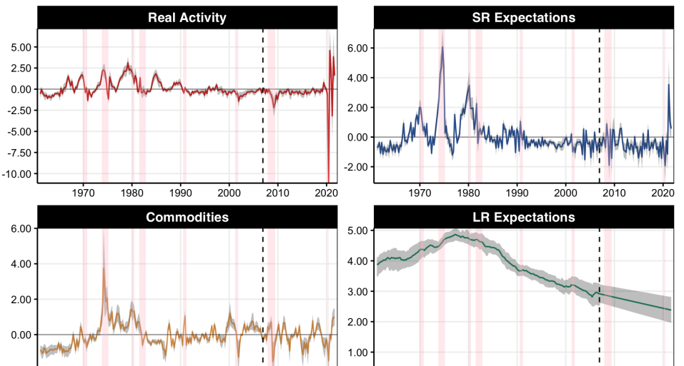
Figure 16: Contributions ($h_{t}$’s) from HNN-F with training ending in 2007. Notes: Dashed line is the beginning of the out-of-sample. NBER recessions are in pink shadowing.

As starting point, $h_{t}$’s are displayed in Figure 2 for a training sample ending in 2019Q4. Figure 16 (appendix) reports largely unchanged estimates from using a training sample ending in 2007. First, we observe large positive contributions of $h_{t,g}$ to $\pi_{t}$ in 1970s and 1980s which have been much more muted since then, in line with the declining PC narrative (this will be formally assessed when looking at $\gamma_{t}$ in Figure 5). But that was before the pandemic. HNN-F and HNN (Figure 15) both report an extremely high positive contribution from $g_{t}$ to $\pi_{t+1}$ starting from late 2020–as projected from a fixed structure estimated up until 2019. As a result, HNN-F’s (and HNN as well) are forecasting annualized headline inflation consistently above 4.5 starting from 2020Q4 (see Figures 4(b) and 7(b)). While this finding lends support for the view that inflation’s comeback was rooted in economic fundamentals (and potentially caused by a cocktail of expansionist policies, blanchard2021defense; goodhart2021may; gagnon2021inflation), it is not entirely inconsistent – at least statistically – with the possibility of the inflation surge ending rapidly. Indeed, contribution and gaps estimates in the Pandemic era move up and down at a much faster rate than that of previous recessions (along, among other things, public health policies), and it seems possible (statistically, at least) that $g_{t}$ closes as fast as it opened. However, as of 2021Q3 data (i.e., excluding the Omicron surge), $g_{t}$ seems now firmly stationed in positive territory. Moreover, HNN’s estimation of $h_{t,g}$ support the growing evidence that the PC is highly nonlinear in traditional economic indicators space and that the steep part of it has simply been unsolicited in recent decades (linde2019resolving; MRF; forbes2021low).

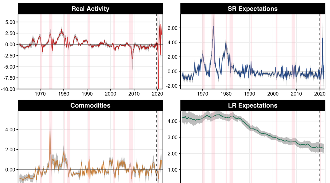
Figure 2: Contributions ($h_{t,j}$’s) from HNN-F. Notes: Dashed line is the beginning of the out-of-sample. NBER recessions are in pink shadowing. Gray shading is the 68% credible region.

$h_{t,g}$ estimates of the last 2 years cast some doubts on methodologies forcing smoothness through laws of motion. Those typically require potential output to trend upward slowly (a random walk, or local-level process) whereas it has been subject to important and rapid downward or upward swings due to "COVID-19 shocks" (blanchard2021defense). Among other things, there are constraints on production that did not exist in 2019 and many Americans have exited the workforce in 2020-2021 not to return just yet. This trend has a name – the Great Resignation – and can be seen in the participation rates as of late 2021. Capturing the conjunction of these phenomena statistically using data through 2019Q4, HNN’s $g_{t}$ is reported in section 4.2 to heavily use a nonlinearly processed Help-Wanted Index–which has hit all-times highs in recent quarters. Further reinforcing the view that $g_{t}$ is as positive as HNN estimates it to be, coming from the demand side, reallocation shocks puts some sectors are under considerable stress for increased production. Also, a significant amount of resources is now dedicated to producing new goods and services (vaccines, tests, etc.) which are partly procured free of charge by governments and do not appreciably crowd out private spending – which itself has been galvanized by fiscal and monetary policies. Thus, private consumption has caught up with its pre-pandemic trend while government expenditures are magnitudes larger than they were back in 2019, making for the total of the two largely surpassing pre-pandemic levels. The purposes of this discussion is not to review every aspect of inflation commentary in 2021 and early 2022, but to highlight that there are plausible economic arguments rationalizing HNN’s seemingly unusual findings – in addition to the plethora of statistical ones reported in this work.

Contribution of the $\mathcal{E}_{t}^{\text{SR}}$ component was extremely strong during the 1970s and has been literally shut down since the beginning of Paul Volker’s chairmanship – at least, until early 2021. The hibernating $h_{\mathcal{E}^{\text{SR}},t}$ woke up, and captures nicely the consequences of supply chain disruptions and the general sentiment in the media and population that inflation could be back. By doing so, it procures relatively accurate inflation forecasts for the turbulent 2021. This will be further discussed in Section 4.1. It appears that the main reason why inflation forecasts did not climb to 1970s levels in late 2021 is $h_{\mathcal{E}^{\text{LR}},t}$, which despite its earlier spike, shows much less persistence than 4-5 decades ago. Said differently, expectations are still relatively well-anchored, by not deviating persistently from the long-run ones.

Additionally, gentle upward spikes are observed post-GR which lend some support to coibion2015phillips’s point that higher expectations following the financial crisis can explain the missing disinflation puzzle. In Figure 19 (from ablation studies in Appendix A.2), this nonlinear pattern is even more apparent from dropping some of the more volatile inputs from $\mathcal{H}_{\mathcal{{E}^{\text{SR}}}}$. Finally, the commodity group (with oil being naturally its most influential member) contributed strongly, to nobody’s surprise, from the first oil crisis of the 1970s, through the second oil shock, and ends after the second of the twin recessions. Finally, $h_{\mathcal{E}^{\text{LR}},t}$ is found to be slowly decreasing, as expected. Note that the overall level of $h_{\mathcal{E}^{\text{LR}},t}$ is not identified separately from $h_{\mathcal{E}^{\text{SR}},t}$ and here it was set by normalizing the other three components to have mean zero over the sample.

Since gaps themselves rather than contributions are what is typically reported, Figure 3 reports contributions from a canonical PC regression for comparison purposes. In the case of "CBO", those are constructed from a traditional PC specification (including 2 lags of $\pi_{t}$ and the gap) with time-varying coefficients obtained from GC2019 two-steps ridge regression approach. Contributions are interesting in their own right because, unlike gaps and coefficients, they are completely identified and expressed in "inflation units". The difference between HNN-F and alternatives is striking for $h_{t,g}$, with the latter giving real activity much less weight in driving inflation than what the former reports. This is especially true in the 1970s and 1980s, but also from recent years. From an ocular spectral analysis standpoint, it is clear that ${h}_{t,g}^{\text{HNN}}$ includes much higher frequencies than what traditional gaps/contributions do. ${h}_{t,g}^{\text{HNN}}$ is prone to rapid spikes that the alternatives completely forego (e.g., the mid-1980s, the years preceding the 1990s recession,and the mid 1990s). It is worth remembering the reader that the frequency range for classical estimators is not an outcome but an assumption – which is explicit in the case of band-pass filters (guay2005hodrick).

"HNN-F CBO", which replaces all the activity data in $\mathcal{H}_{g}$ by the CBO gap itself – thus keeping all the other modeling ingredients from HNN – partly helps in understanding this wedge. Indeed, the green and red line follow each other closely each except following the 1981-1982 and 2008-2009 recessions. "HNN-F CBO" seems to use nonlinearities to avoid to the two very negative contributions from the PC regression. Nonetheless, it is clear that a key difference between HNN and the canonical regression is the nonlinear processing of a rich real activity data set. Finally, only the classic PC regression and chan2016’s gap (CKP) calls from a deep and lasting negative output gap following 2008. "HNN-F CBO" circumvent it interacting with a small implicit $\gamma_{t}$ and HNN follows a very different pattern where the gap closes rapidly (as early as 2011) but remains gently in negative territory at least until 2018. Finally, from the early 1990s up until the GR, both "CBO" and "CKP" contributions are practically 0 whereas HNN-F sees a mild downward contribution from real activity in the years surrounding the 2001 recession.

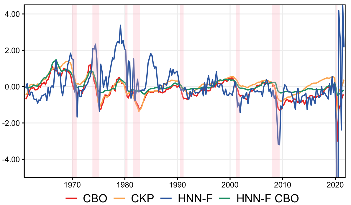
(a) Contributions of economic activity to inflation.

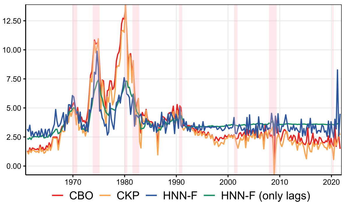
(b) Contributions of expectations to inflation.

Figure 3: Comparing estimated contributions. Notes: all estimations end in 2019 and are projected using the out-of-sample data from there. Pink shading is NBER recessions. "CBO" is the estimated contribution from a PC regression using the CBO output gap as forcing variable. CKP means the estimated contribution as extracted from chan2016’s model. "HNN-F CBO" means that all the data entering $\mathcal{H}_{g}$ was replaced by the CBO gap (and keeping $t$) and an HNN was rerun. "HNN-F (only lags)" means that all the data entering $\mathcal{H}_{\mathcal{E}}$ was replaced by lags of $\pi_{t}$ (and keeping $t$) and an HNN was rerun. In the case of expectations, $\mathcal{E}_{t}^{\text{LR}}+\mathcal{E}_{t}^{\text{SR}}$ is plotted for HNN and the plot for "CBO" is the sum of the two lags plus the time-varying intercept. Analogous calculations are carried for CKP.

HNN’s current estimates differ even more dramatically from that of standard techniques. CKP’s gap in Figure 5 behaves like most unemployment filtering methods do. It reports strong overheating in the late 2010s and a gently positive gap in late 2021. As we will see in the forecasting results of section 4.1, this will be largely insufficient as upward forcing to obtain well-centered forecasts during that period. This is no surprise: this approach yields an output gap which is mostly negative throughout the Pandemic and the PC coefficient is small. berger2020nowcasting’s multivariate approach reports online a positive gap as of January 12th 2022 that is comparable in size to that of the end of the last two expansions (unlike HNN which sees mostly unprecedented inflationary pressures starting from 2020Q4). Also, hazell2020slope (and their updated estimates here) utilize an extremely persistent ARMA(2,1) output gap (looking very much like filtered unemployment), which allegedly pushes the model to explain the data with an energy price cycle. As per Figure 2 (and eventually even clearer in Figure LABEL:graphs_hnns), the direct role of commodity prices has become more muted in recent years – a finding likely due to HNN allowing for a more flexible $g_{t}$. This debate is important: different decompositions imply different policy recommendations. While HNN $h_{t,g}$’s unequivocally calls for a tightening of monetary policy, during times of sectoral reallocation, the divine coincidence is broken, leading to an "optimal" level of inflation that is easily above the target (guerrieri2021monetary). Obviously, letting inflation sit for a while above the target range comes at the risk of disanchoring expectations which were anchored at great cost long ago.

In Figure 3(b), it is striking that, unlike Figure 3(a), HNN and its altered version form a cluster. This suggests that the information contained in $\mathcal{H}_{\mathcal{E}}$ beyond lags of $\pi_{t}$ only seldom makes a difference — although it makes all the difference for latest inflation upswing. It is also obvious that HNNs allocated a much smaller fraction of inflation to expectations, which is particularly visible from the 1970s inflation spirals (mostly the second) and the 1980s. One way to explain this is that a mispecified $g_{t}$ led to put an excessive burden on explanation on $\pi_{t}$ lagged values.

(a) Absolute Contributions to $\hat{\pi}_{t}$

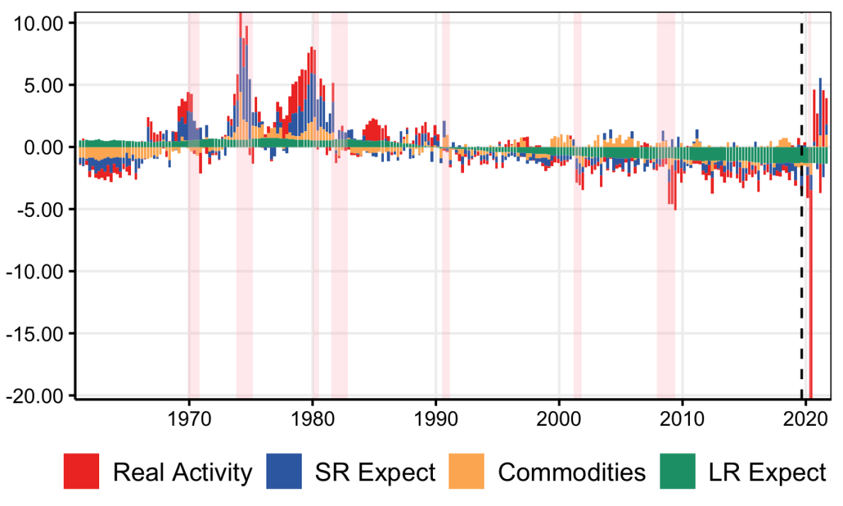
(b) $\hat{\pi}_{t}$ decomposition

Figure 4: Summed contributions from the four $\mathcal{H}$’s through time. Notes: all estimation ends in 2019 and are projected out-of-sample from there. For the specification details yielding "CKP" and "CBO" estimates, see notes of Figure 3. Pink shading is NBER recessions.

Figure 4 reports inflation shares in two ways. In Figure 4(a), the decline of the overall influence of $\mathcal{E}_{t}^{\text{SR}}$ in favor of $\mathcal{E}_{t}^{\text{LR}}$, with the emergence of trend inflation dominance in the mid-1990s. $\mathcal{E}_{t}^{\text{SR}}$ peak contributions are with the 3 inflation spirals of the 1970s, and to a lesser extent the mild increase from the end of the 1980s. The share of $h_{t,g}$ is much more stable than what typically reported by PC regressions although it appears to be milder (in a very subtle fashion) starting from the 2000s. The effect of energy and commodity prices appears stable. Figure 4(b) makes clear that key historical increases are always due in large part to $\mathcal{E}_{t}^{\text{LR}}$, including that of 2021. A key pattern is an initially mild positive contribution from $g_{t}$ followed by a large and lasting upswing in the blue component.

HNN successes and failures in forecasting post-2019 inflation can be easily understood from Figure 4(b). The "overkill" downswing is entirely due to the real activity component, and the increase in first half of 2021 is due to a pattern very similar to the 1970s being replicated, that is, a gentle positive impulse from $g_{t}$ followed by a sizable upward pressure from $\mathcal{E}_{t}^{\text{SR}}$. A noteworthy observation is that $\mathcal{E}_{t}^{\text{SR}}$ appeared dormant until 2021, like in the "PC reg" and "HNN (only lags)" specifications of Figure 3(b), while it truly was not. Its spectacular awakening from nearly 3 decades of hibernation, most likely due to unsolicited nonlinearities now being useful, is what makes HNN forecasts of 2021 on point whereas other PC-based forecasts fail — their coefficients are so weak that resulting forecasts often look close to straight lines.

So far, the focus has been on $h_{t,g}$. As discussed in Section 2.2, HNN-F allows for a separate inspection of $g_{t}$ and $\gamma_{t}$. Figure 5 reports them for the estimation ending in 2019Q4. Unlike recessions that preceded it, the GR is characterized by a rapid yet incomplete closing of the gap. Interestingly, this mildly negative gap lasting for a decade coincides in part with the so-called missing inflation era. This observation – a rapidly closing gap followed by a long slightly negative one – is found whether we estimate the model using data up to today, or end estimation in 2007. Thus, HNN-F is not reverse engineering a $g_{t}$ to fit the post-GR inflation data. Moreover, the rapid closing of $g_{t}$ following the GR is not observed for the early 1990s and 2000s recessions. This distinction is even clearer when using the less volatile Core CPI as supervising variable in Figure 9. Thus, what is observed for $g_{t}$ in the early 2010s is not due to it always closing faster, perhaps in a mechanical way.

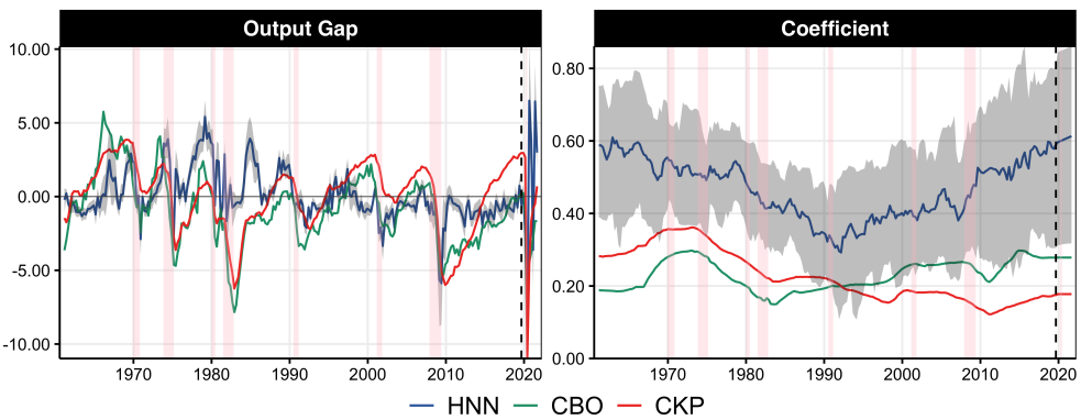
Figure 5: HNN-F’s gap ($g_{t}$) and associated coefficient ($\gamma_{t}$). Notes: Dashed line is the beginning of the out-of-sample. NBER recessions are in pink shadowing. Gray shading is the 68% credible region. See Figure 3 for specifications details.

What about $\gamma_{t}$, the widely studied evolving coefficient of the PC? The evidence in Figure 5 is in partial agreement with the recent literature on the matter (blanchard2016phillips; gali2015monetary; del2020s) in the sense that the exogenously time-varying $\gamma_{t}$ has been decreasing. However, there are many notable differences. First, there seem to be a break around 1980, in the midst of Volker disinflation, where $\gamma_{t}$ ’s decline substantially accelerates. Second, unlike results from standard approaches, $\gamma_{t}$ is not found to decline further following 2008, but rather to increase gently. Results including COVID-19 data suggests an even stronger pickup of HNN-F’s $\gamma_{t}$ in the last 12 years. These observations are in sharp contrast with blanchard2016phillips’s findings using a (supervised) filtered unemployment gap. They report a slowly decaying $\gamma_{t}$ that gets even closer to 0 following the GR, which is very close to CKP-based results (the red line) obtained in Figure 5. stock2019slack report very similar results for a plethora of slack measures (albeit all of them being strongly correlated with each other), with coefficients being all in the vicinity of 0 for the 2000-2018 period. Also using unemployment as real activity indicator but identifying $\gamma_{t}$ with cross-sectional variation (US States), hazell2020slope also find a small PC coefficient. Given how different HNN-F’s $g_{t}$ is with respect to traditional detrended GDPs, filtered unemployment, and other neighboring alternatives, $\gamma_{t}^{\text{HNN}}$ atypical vivacity is not entirely surprising. All in all, HNN-F results suggest that, yes, there exist a measure of slack which effect on $\pi_{t+1}$ has been appreciable and mostly stable over the last 4 decades —and that is not filtered unemployment.

A relevant statistical question is whether HNN could be prone to rewriting history — because many of the gap estimation methods based on plain filtering are (orphanides2002unreliability; guay2005hodrick). Figure 6 suggest that HNN-F’s estimation of $g_{t}$’s to be rather stable, with the qualitative patterns observed in Figure 5 being completely intact. There are some mild quantitative disagreements between the 2000 version and the remaining four, especially for the positive $h_{t,g}$ preceding the crisis. As for the aftermath of the crisis and the 2010s, there are some mild quantitative disagreement but the pattern – strikingly different from those of traditional methods – is the same across specifications. That is, we get a major but short-lived dip following the crisis, a brief comeback to 0, then a long mildly negative phase up until 2018. All estimations agree on economic pressures on inflation increasing from the mid 2010s up until the Pandemic., with a slight disagreement on the overall level of $g_{t}$. Historical results are robust to the inclusion/exclusion of wild pandemic observations and $g_{t}$ movements are rather similar whether they are projected out-of-sample from 2019 or using all the data up until today. The quantitative discrepancy between the 2019 and the full-sample versions is obviously larger during 2020, but so is estimation uncertainty. The 2020-2021 data has the effect of dampening the gaps movement in the last 2 years because the algorithm attempts to minimize (now in-sample) the large forecast error for 2020Q3, an observation that should be in fact discarded with dummies. Overall, results with training ending in 2019Q4 were preferred as benchmarks since COVID-19 observations have an extremely high level of volatility attached to them and one simple way to statistically account for that is to drop them (lenza2020estimate; schorfheide2020real). Moreover, it allows to evaluate whether a statistical model that has not seen 2021.

Figure 6: $g_{t}$’s estimated on various training sets. The left panel is zooming on the $[-7.5,7.5]$ range of the right panel.

Many ingredients enter HNN for it to deliver the gap and expectations reported in this section. Dispensing with some of them helps in understanding the respective contribution of each. In Appendix A.2, I conduct an ablation study where HNN is deprived, in turns, of the large data set and the nonlinear supervised processing. In short, the combination of both appears essential. For instance, one could wonder if the use of a data set partly populated by growth rates – rather than levels or deviations from them – could have been a factor behind HNN’s success that has little to do with HNN itself. It turns that no: the linear unsupervised processing of the same data set produces a $g_{t}$ that remains below 0 or in the vicinity of it throughout 2021.

4.1 Forecasting

4.1.1 Setup

The pseudo-out-of-sample period starts in 2008Q1 and ends 2021Q3. I use expanding window estimation from 1961Q3. HNNs are re-estimated and tuned every 4 quarters. Following standard practice, the quality of point forecasts is evaluated using the root Mean Square Error (MSE). For the out-of-sample (OOS) forecasted values at time $t$ for $s\in\{1,4\}$:

$$RMSE_{s,m}=\sqrt{\frac{1}{\#\text{OOS}}\sum_{t\in\text{OOS}}(\pi_{t:(t+s)}-\hat{\pi}_{t,s})^{2}}.$$

Three targets are considered. First, CPI($s=1$), which is the supervisor in the benchmark HNN specifications. Additionally, the alternative supervisors eventually studied in Section 4.3 – CPI average inflation from $t$ to $t+4$ (${\pi}_{t:(t+4)}=\sum_{s^{\prime}=1}^{4}\pi_{t+s^{\prime}}$) and Core CPI($s=1$) – are considered. Performance results are reported including and excluding 2020 observations. As we will see in Section 5, while NNs in general provide erroneous forecasts for 2020Q3 and 2020Q4, an extended HNN-F which models both the conditional mean and the conditional variance predicts unprecedented levels of imprecision for those two forecasts. In contrast, HNN-F is as confident as it gets for the 2021 projections. Thus, using that timely information, a forecaster would have discarded 2020 forecasts ex-ante (but not those of 2021) in a similar fashion to what the barplots of this section are doing ex-post.

A few obvious benchmarks from both sides of the aisle are considered. On the ML side, there is a fully connected neural network with the same hyperparameters as HNN (DNN) and a random forest (RF) with default tuning parameters (typically hard to beat). They all use the exact information set as HNN (variables and aforementioned transformations). Then, there are inflation-specialized econometric benchmarks of increasing sophistication. First, we have the AR(4) which will stand as the generic numeraire of reported MSEs. Then, two rolling means are considered, the one-year mean à la atkeson2001phillips (1y Avg) and a longer-run one (10y Avg). Bringing in real activity information in, I consider a PC regression (PC, two lags of $\pi_{t}$ and the CBO gap) estimated on a rolling window of 15 years to allow for time-varying parameters. Note that this PC reg is given a handicap by using the latest CBO gap which may have been substantially revised ex-post — and after observing inflation, the forecasting target. Additionally, an identical PC regression augmented with two lags of oil prices and survey expectations (PC+) is considered to match some of the information set in HNN, and more generally specifications inspired from coibion2015phillips. Finally, we consider chan2016’s time-varying bounded Phillips curve model (CKP) where $g_{t}$ is extracted in a supervised fashion from unemployment by assuming the natural rate of unemployment to follow a random walk. Key coefficients also follow random walks. This approach was reported to have sporadic success in forecasting euro area inflation (banbura2020does) and could be seen as the state-of-the-art Bayesian method to forecast inflation based on some form of gap. All those non-NN methods are re-estimated every quarter.

4.1.2 Results

I now report the forecasting performance of HNNs for the three targets and look at their forecasts. In Figure 7(a), HNN and HNN-F are shown to perform well –when excluding the aberrant 2020 observations. In Figure 7(b), we understand that HNN’s relative success is due in part to capturing with reasonable accuracy the recent upswing in inflation. Of course, this achievement is counterbalanced (within all of out-of-sample) by overly pessimistic forecasts following the dip of 2020. On the other hand, HNN was not communicated of an unprecedented government-induced economic shutdown, and a careful use of the model would have discarded the downward spike.

For the 3 targets, HNN and HNN-F forecasts are very close to one another throughout the out-of-sample. Notable exceptions are the 4 recent quarters for CPI($s=1$) and Core CPI($s=1$) where HNN delivers very accurate forecasts and HNN-F performance lives somewhere between that of HNN and PC+. Nonetheless, both models predict $\pi_{t+1}$ being above the target range starting from 2021Q1. While a certain potency during 2021 is common to all deep networks, DNN’s predictions (unreported), while broadly getting the upward "trend" right, are volatile and are either too high or too low. During the same period, PC+ visibly acts as an autoregression, pushing the forecast upward according to previous positive shocks. Additionally, it wrongly calls for largest immaterial deflation in the aftermath of 2008, which is, in effect, a classic failing of regression models predicting inflation with an output gap. HNN and HNN-F are not completely exempted from this failing for CPI($s=1$) but avoid this predicament CPI($s=4$) and Core CPI($s=1$). One explanation is the rapid closing of HNN’s gap, for all three supervising variable (see Figure 9 and its discussion in Section 4.3). The other emerges from Variable Importance results of Section 4.2. Another modern approach is CKP, based on a Bayesian bivariate state-space model of trend inflation and the gap. Its reliance on unemployment appears fatal in two historical episodes. First, its forecasts are consistently too low for most of 2008-2012. Second, its forecasts remain significantly below realizations for all of 2021. The reason for this is self-evident from Figure 5: de-trended unemployment rate, the forcing variable, is negative for most of 2021. Thereby, if it forces in any direction, it is downward, not upward.

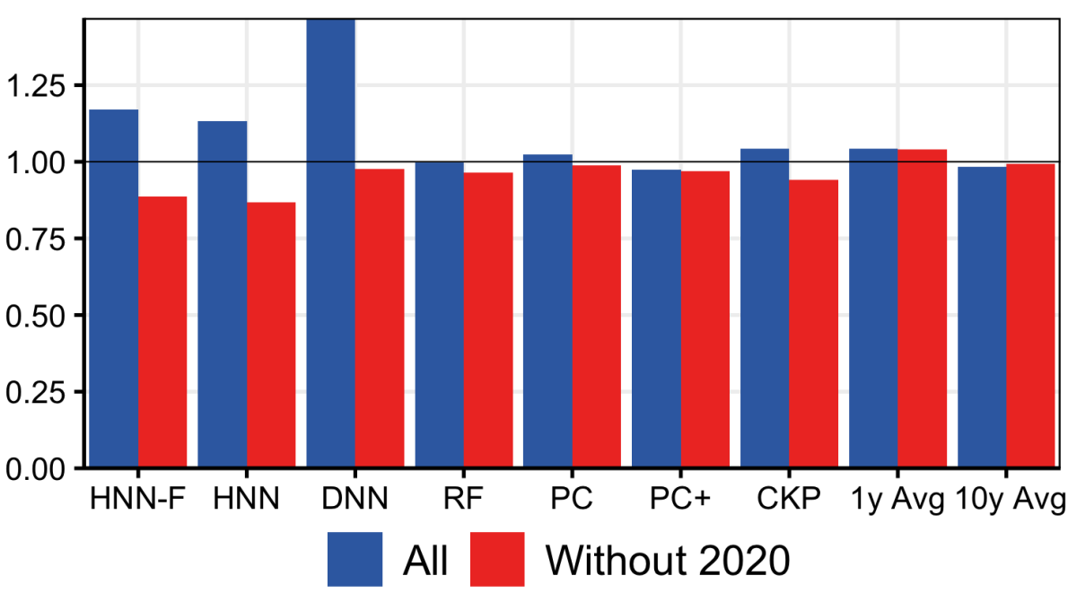
(a) MSE wrt AR(4), CPI

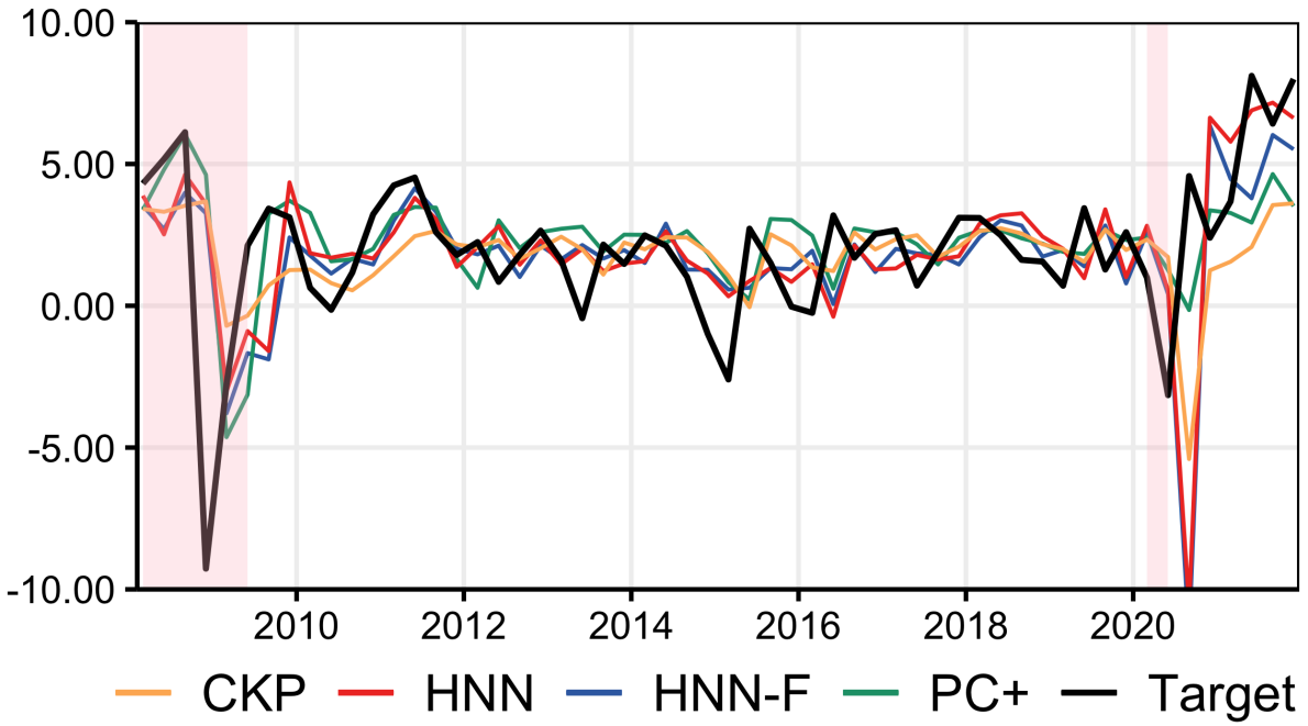
(b) Forecasts, CPI

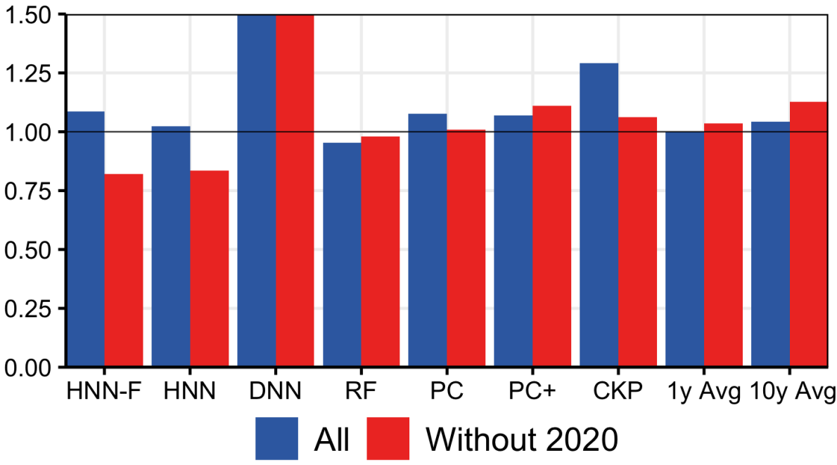
(c) MSE wrt AR(4), Core CPI

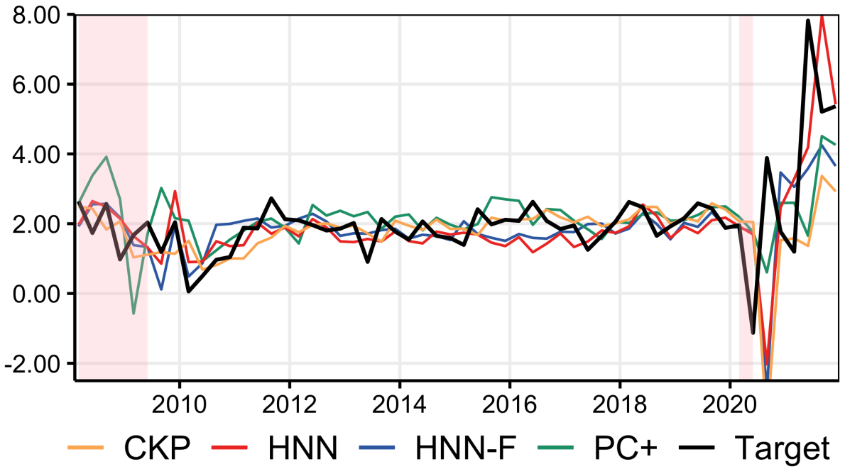
(d) Forecasts, Core CPI

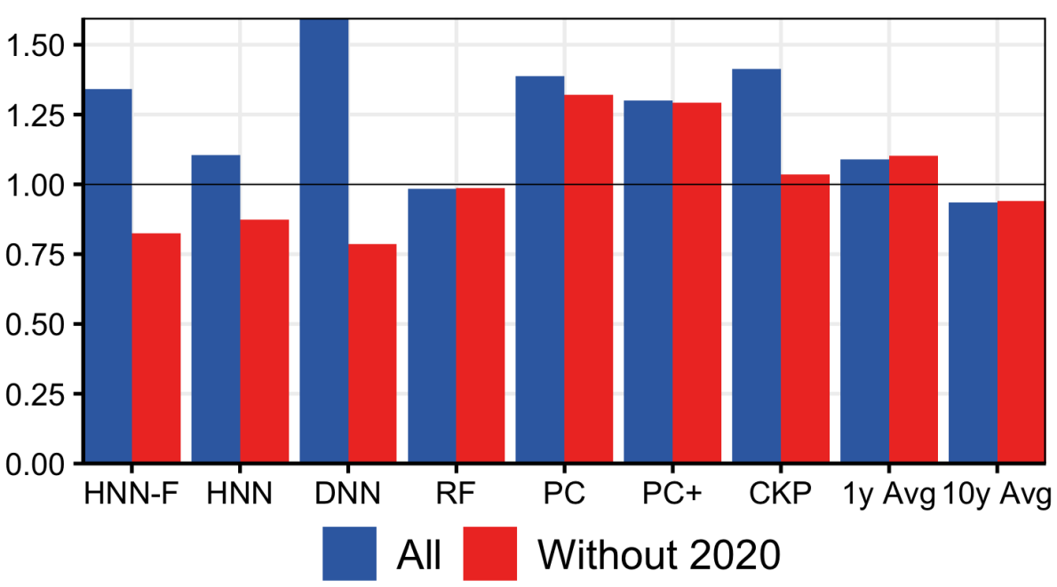
(e) MSE wrt AR(4), CPI ($s=4$)

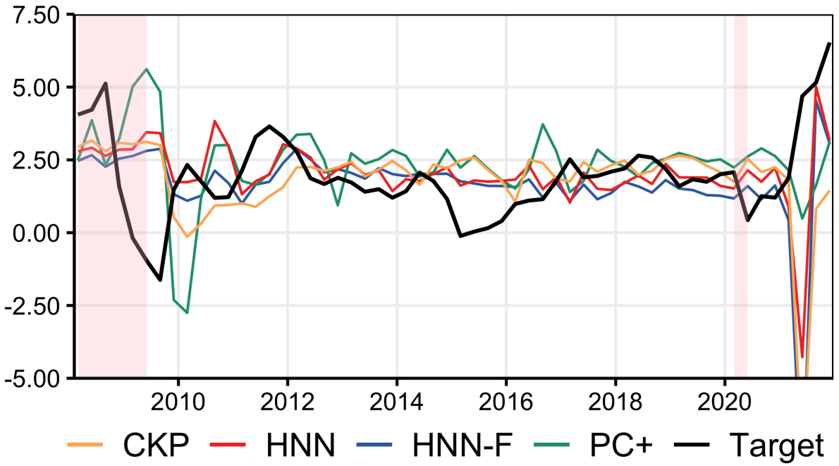
(f) Forecasts, CPI ($s=4$)

Figure 7: Forecasting Results for 3 targets with test set 2007Q2-2021Q4 and re-estimating NNs every year. Notes: Pink shading is NBER recessions.

Turning to Core CPI, we again see that, leaving out 2020 data, HNNs have the lowest MSEs. It is noteworthy that the extent of the "2020 forecasts demise" is much smaller for core inflation. HNN captures reasonably accurately what is, at least since the 1990s, a rise in Core CPI that is unprecedented in both speed and magnitude. Similarly to headline CPI results, CKP forecasts are again too low.

For one-year ahead forecasts, Figures 7(e) and 7(f) reveal that HNN and HNN-F provide the best PC-based forecast in the lot, again, when excluding 2020. As mentioned earlier and explored in detail in section 5, this exclusion can alternatively be motivated from an augmented HNN itself recognizing that its forecasts are very likely unreliable. Unlike PC+ in Figure 7(f), HNN-F and HNN are not lured into predicting long-lasting disinflation (or even deflation) following the GR— because HNN-F’s gap is closing as fast as that of the benchmark CPI($s=1$) estimation and $\gamma_{t}$ is moderately small (see Section 4.3). This, however, does not prevent HNNs from displaying the Phillips curve relationship in all its vivacity when needed. While NN-based forecasts are more dispersed for this target, they agree on one thing, an average CPI inflation of 4% from 2020Q4 to 2021Q3 inclusively, which is well above target. In contrast, PC+ calls for a timid 2.5% and CKP expects inflation to be below the target. The closest competitor is the atheoric 10 years mean. While their associated MSEs are relatively close, forecasts differ substantially, with HNN-F channeling information about real activity whereas the rolling mean does what a rolling mean does, i.e., a semi-flat line.

Unsurprisingly, yearly results for 2020 and most of 2021 are not great for any real-activity-based forecasts, including HNN. In a similar fashion to what reported in Figure 7(b), this is due to HNN and PC regressions not being informed that this is no ordinary recession and that extraordinary governmental programs have been implemented to life support the economy. This limitation has even stronger consequences when forecasting ${\pi}_{t:(t+4)}$ since the medium-run dynamic transmission mechanism itself is certainly quite different during the Pandemic than for previous recessions. In other words, due to an imminent structural break, it is not shocking that HNNs or PC regressions are over-pessimistic in the initial and most of the subsequent response of ${\pi}_{t:(t+4)}$ the COVID-19 shock. On top of that, one-year ahead inflation is particularly subject to the various pandemic plot twists which can occur within four quarters.

Overall, barplots of Figure 7 show improvements ranging from 10% to 25% when excluding 2020 observations, with HNN-F and HNN always delivering comparable RMSEs. For all 3 targets, the closest competitors in terms of RMSE are the rolling 10 years mean, PC+ (which includes the survey of professional forecasters’ forecast as a predictor), and sometimes Random Forest. For the former, it is not an uncommon result, especially for a period of relative stability in the 2010s — and avoiding the perils of calling missing disinflation by construction. But those forecasts cannot capture what crucially matters for policy: when inflation gets out of its target range. Additionally, any form of macroeconomic rationale (except that of anchored expectation) is evacuated from those forecasts. Same is true of the various AR or ARMA configurations. This is, in great part, what still motivates the use of PC regressions despite their well-documented failings (yellen2017inflation). Thus, all in all, HNNs fare well by providing reliable forecasts that have economic soundness and can predict that $\pi_{t}$ will exit the target range before it does.

4.2 What are the gap and expectations made of?

Unlike simpler data-poor $g_{t}$ estimates – where the modeler decides which variables matter ex-ante – or data-rich linear ones – where nonlinearities are typically pre-specified (e.g., trend-cycle decomposition) and we can look at the factor model’s loadings – that of HNN needs additional computations to understand what it is made of. By construction, $g_{t}$ and $\mathcal{E}_{t}^{\text{SR}}$ are combinations of thousands of parameters nonlinearly processing many regressors. Consequently, looking at network weights by themselves is inherently meaningless. More productively, I investigate which $X_{t,k}\in\mathcal{H}_{g}$ seems to matter most by designing a variable importance (VI) exercise very much inspired from what MRF studied for "generalized time-varying parameters" in a random forest context – which is itself inspired from traditional variable importance measures for tree ensembles predictions.

I focus on groups of variable $k$, meaning we will evaluate the overall effect of all transformations and lags of variable $k$ (as mentioned in section 2.1, we include 4 lags of each and moving averages of order 2, 4 and 8). The variable importance procedure to evaluate the relevance of variable $k$ to $h_{t,j}$ can be summarized as follows. $\text{VI}_{k}^{j}$, for a variable $k\in\mathcal{H}_{j}$, works in three steps. First, we shuffle randomly variable $k$ (and all its attached transformations, i.e., lags and MARXs). Second, we recompute (but do not re-estimate) the component $h_{j}(\tilde{X}_{t})$ (using the shuffled data for $k$ and the original data for all other variables). Third, we calculate its distance to the real component estimate $h_{j}(X_{t})$. Formally, the standardized $\text{VI}_{k}^{j}$, in terms of % of increase in MSE, is

$$\text{VI}_{k}^{j}=100\times\left(\frac{\tfrac{1}{T}\sum_{t=1}^{T}(h_{j}(\tilde{X}_{t})-h_{j}(X_{t}))^{2}}{Var(h_{j}(X_{t}))}-1\right).$$ (7)

Intuitively, randomizing important variables will push $h_{t,j}$ further from its original estimate than randomizing useless ones.

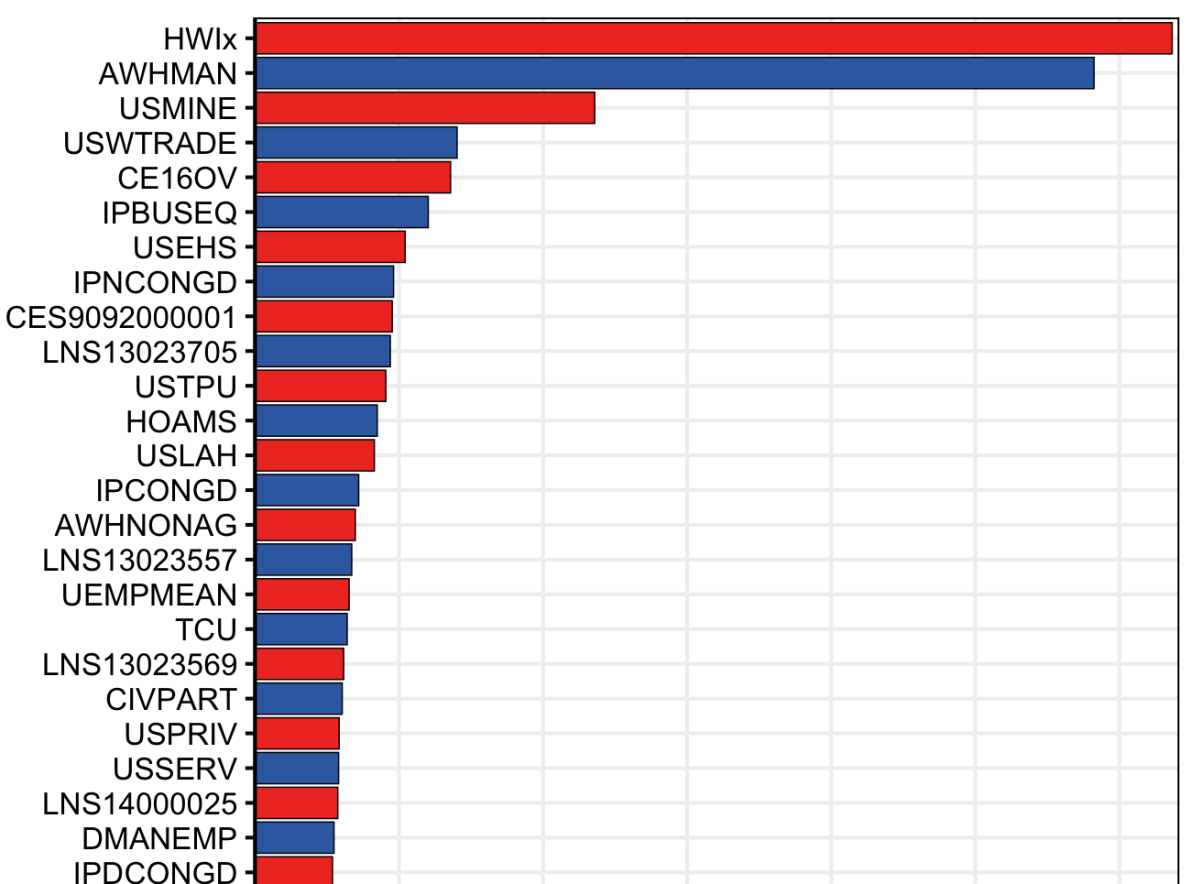
(a) Gap ($g_{t}$)

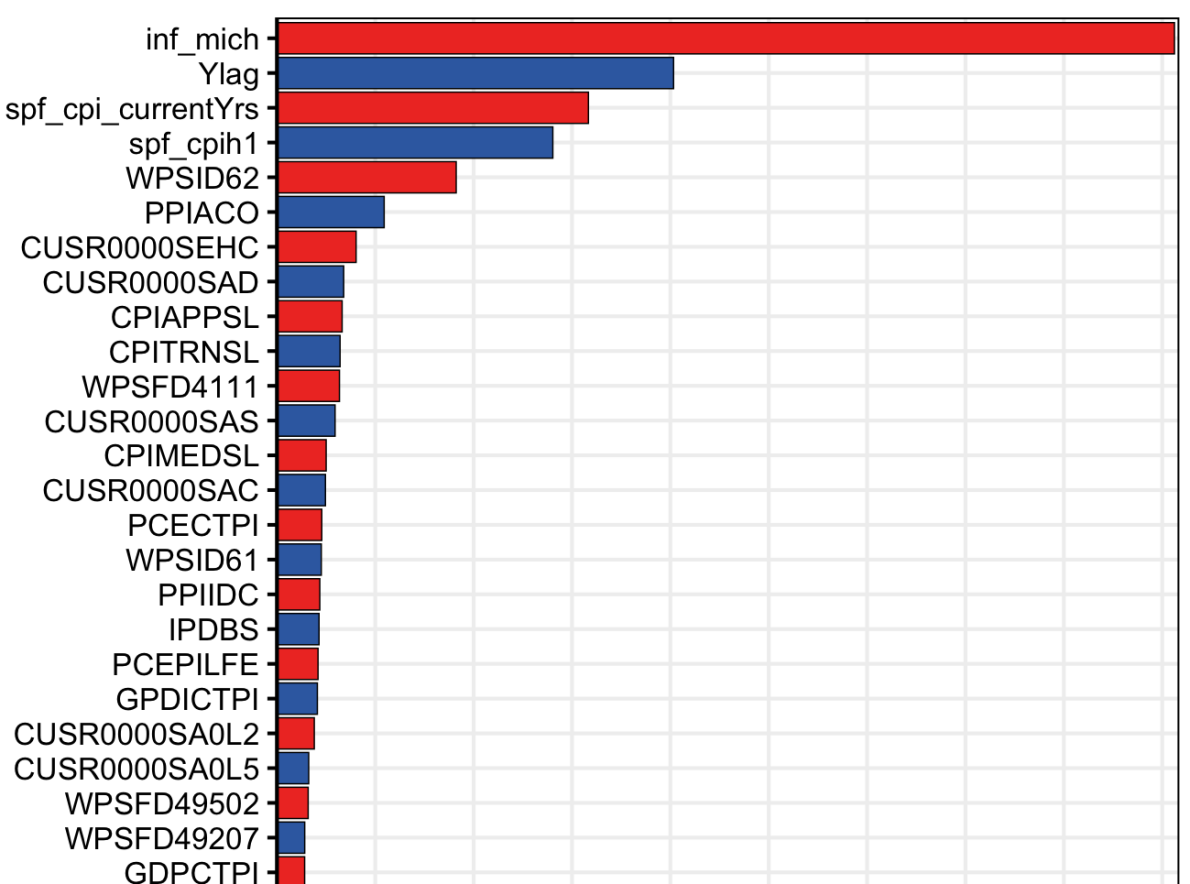
(b) Short-Run Expectations ($\mathcal{E}_{t}^{\text{SR}}$)

Figure 8: VI Results for benchmark HNN-F specification, with training ending in 2019Q4. Mnemonics are those of FRED-QD (mccracken2020fred).

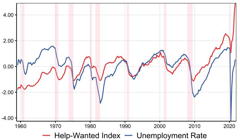
Figure 18: Compared (standardized) measures of slack. Unemployment was multiplied by -1.

VI results are reported in Figure 8. Here are key observations for $\text{VI}^{g}$. First, AWHMAN’s (average weekly hours in the manufacturing sector) predominance for $g_{t}$ suggest an important for the intensive margin, whereas typical labor-based gap measures are mostly about extensive margin (like filtered unemployment). Recently, bulligan2019adjustments find the former can complement the latter as forcing variables in linear PCs for Euro area (but not the US). Second, the composite Help-Wanted Index (HWIx) of barnichon2010building –which mccracken2020fred splice earlier in the sample with the original Conference Board product for "print" job postings – is shown to play an important role. Intuitively, the index, by construction, characterizes increased labor demand (and perhaps shortages) which is expected, by economic theory, to translate in higher wages, and eventually, higher aggregate prices. This partly explains the very positive gap in Figure 5 since HWIx is effectively skyrocketing as of late 2021 despite being largely stagnant in 2018 and 2019. However, this not the whole story: nonlinear neural processing of HWIx seems essential as reported in the ablation study (Appendix A.2). In Figure 18 (Appendix), we see that, at times, the unemployment rate and HWIx were closely related, like during 1990s and the 2000s. But other times they were not, like the 1970s and in a very striking fashion, right now. Moreover, their acceleration rate can differ in key recession and expansion episodes. By putting its money on some transformation of HWIx , HNN leveraged historical patterns to avoid relying on less potent forcing variables. As we now know, those are directly responsible for the failure of traditional PC forecasts in 2021 (Figures 5 and 7).

Remaining variables that are marginally more important than the rest are typically related to employment levels in different sections. Third, GDP and associated measures seem unimportant, so is the unemployment rate. The only traditional gap measure making an appearance in $\text{VI}^{g}$’s top 25 is total capacity utilization (TCU), which, interestingly, is also the one among them delivering (after some filtering) the fastest closing of the gap following the great recession in stock2019slack (see their Chart 3).

Turning to $\text{VI}^{\mathcal{E}_{\text{SR}}}$, we see that a handful of very familiar variables dominate the top 25. First, the obvious preponderance of the University of Michigan Survey of Consumer Inflation Expectations (inf_mich) strengthen the case for the increasingly popular practice of using survey expectations in PC regressions (binder2015whose; coibion2015phillips; coibion2018formation; meeks2019heterogeneous). It also completes the explanation as to why HNN-F forecasts did not call for lasting disinflation following the GR. That is, as suggested by coibion2015phillips, proxying expectations using survey expectations rather than, say, lags of the CPI, procures more accurate post-2008 predictions. HNN learned that prior to 2007 by putting a high weight on inf_mich. Nonetheless, $\text{VI}^{\mathcal{E}_{\text{SR}}}$ suggests mixing in expectations from different economic agents and formulated for different horizons seems more appropriate, which is in line with recent results for simpler regression models in banbura2021inflation. There is also a minor role for "backward-looking expectations" or "inflation persistence" as characterized by the presence of lags of the CPI (Ylag) in the top 4.

Lastly, we see the overall producer price index (PPIACO) and the PPI for crude materials for further processing (WPSID62) being marginally more important than the remaining variables. These contribute information about cost-push shocks that producers will eventually pass in part to consumers. These enter the model in second-differences of the log (following the transformation suggested in mccracken2020fred) and thus represents "acceleration rates". Looking at those time series reveals that the highest acceleration on record (since 1960) was recorded for both variables in the third quarter of 2020. Consequently, the visually obvious spike (that is not necessarily unique to those two series) is arguably what is driving the flash disanchoring of ${\mathcal{E}_{t}^{\text{SR}}}$.

4.3 Changing Supervisors

The deep output gap and associated results from HNN have been learned through supervision with headline inflation. Changing supervisors could alter results. For instance, it has been reported recently and less recently that alternative measures of inflation – typically stripped-down version of the CPI designed to be less volatile – can deliver different results, for instance, about the strength of the PC (morel2013common; ball2019nonpuzzling; stock2019slack; luciani2020common). Making a deep dive in the pool of alternatives CPI is left for future work, but investigating trivial alternatives can be informative on the robustness of $g_{t}$ and the mechanics of HNN. In this section, I report $g_{t}$’s and $\gamma_{t}$’s obtained from HNN-F with two alternative supervisors that were introduced in the forecasting experiment (Section 4.1). The first is Core CPI (headline minus food and energy). The second is the average inflation rate over the forthcoming year. Tuning and architecture details remain intact from Section 2.3, except that dropout is turned off for these two less noisy targets.

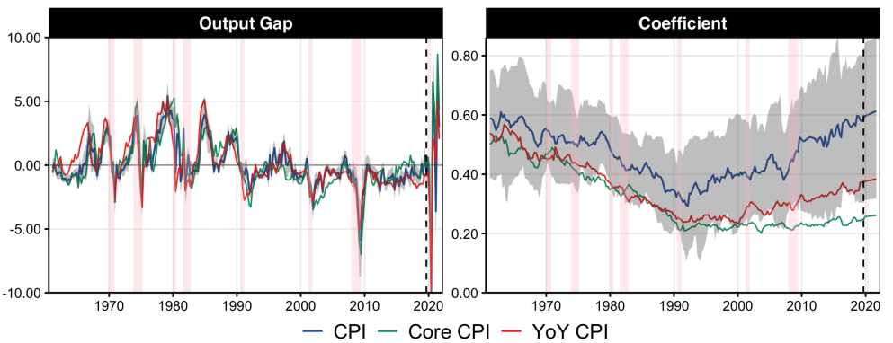
Figure 9: HNN-F gaps and associated coefficients with alternative supervisors. Notes: Dashed line is the beginning of the out-of-sample. NBER recessions are in pink shadowing. Gray shading is the 68% credible region.

Estimation results reported in Figure 9 are suggestive that there is such a thing as a unique real activity latent state driving future inflation for various horizons. All ${g}_{t}$’s follow a clear common pattern, with that of yearly inflation showing larger amplitudes than one quarter ahead $\pi_{t}$ up to 1990, and that Core CPI being slightly less. All gaps close relatively slowly following the early 2000s recession (with Core CPI’s gap closing the slowest of the 3) and all close extremely fast following the GR. They also share a common arc-shaped mildly negative gap from 2011 to the onset of the COVID-19 era. During the pandemic, the general pattern is again common to all three but magnitudes differ substantially, in line with the wide uncertainty of the last two years. For instance, ${g}_{t}$ obtained from CPI (benchmark) is dissenting from those of CPI Core and YoY CPI by calling for a negative gap in 2021Q2 . The other two ${g}_{t}$’s remain (very) positive from the end of 2020, which is the basis for their respective upward forecasts in 2021 reported in Figure 7.

In terms of coefficients ($\gamma_{t}$’s), those are typically lower for both alternatives supervisors, and so is their revival in the 2000s, with that of ${\gamma}_{t}^{\text{Core}}$ being practically non-existent. Credible regions suggest slack’s contribution to inflation is similar for the CPI at $s=1$ and $s=4$. ${\gamma}_{t}^{\text{Core}}$’s overall level suggests a slightly lower passthrough from real activity to core inflation. Nevertheless, the main message from the previous section stands still: there is a nonlinear measure of real activity which still impacts inflation greatly and drives current (mostly on-point) forecasts – much more than what one may obtain from a plethora of classical gaps.

In Appendix A.3, a more radical departure from the benchmark specification is conducted with the federal fund rate replacing inflation as supervisor. Accordingly, this last gap is extracted from a Taylor rule rather than a PC and will represent the $g_{t}$ the Fed "has in mind". Interestingly, the resulting gap looks more like a traditional filtered one, suggesting there may a gap between the monetary authority’s view of economic slack (in line with typical econometric estimates used by economists) and what can rationalize the inflation record.

5 Can HNN Predict its own Demise? On Inflation Volatility

In comparison to trademark AI applications like image recognition and machine translation, the signal-to-noise ratio is low for most economic applications. This means that a predictive algorithm is fallible to an extent where it becomes useful to also predict volatility — i.e., when it is more likely to miss its target by larger margins. Econometricians know that all too well and have proposed a suite of models for conditional heteroscedasticity which have been used extensively in macroeconometrics and financial econometrics, with stochastic volatility (SV) and (G)ARCH being respectively the leading paradigms (engle1982autoregressive; jacquier2002bayesian). In the case of inflation, the unobserved components model with stochastic volatility (UC-SV) has been popular for forecasting purposes (stock2007has) and the time-varying parameter vector autoregression with SV for structural analysis (primiceri2005).

An important roadblock is that those options are not readily implementable without deviating significantly from the highly-optimized software environments that make HNN computations trivial. SV requires Bayesian computations and appears restrictive in the kind of variation it allows for, especially when compared to the conditional mean function. As a result of it being essentially a trend-filtering problem for squared residuals, it is unequipped to detect future volatility spikes in the target series–although it can be adjusted to deal with outliers after the fact carriero2021addressing. Implementing GARCH-like volatility within HNN would be similarly daunting given that the MLE estimation of simple GARCH models is already challenging in itself (zumbach2000pitfalls; zivot2009practical). Approaches alternating the fit of the conditional mean and the conditional variance until convergence – à la iterated weighted least squares – are also highly impractical. First, the DNN residuals within the training sample can easily be reduced to dust (belkin2019reconciling), making them an unusable target in a secondary conditional variance regression. Second, it is sometimes difficult to get a single DNN to converge, so alternating between two of them will unlikely deliver. Lastly, the many bells and whistles of gradient descent (like the Adam optimizer) can make a sizable difference. Thus, there is great statistical and computational cost in deviating from the current implementation of HNN or DNNs in general.

Would not it be nice if it were possible to merely create an additional volatility hemisphere, and carry HNN estimation practically as is? As it turns out, it is – and only requires changing HNN’s loss function. The key insight is that spady2018simultaneous’s simultaneous mean-variance linear regression can be generalized by a HNN with a marginally more sophisticated loss function (GC2022). For the current application, the least squares problem is replaced by

$$\min_{(w_{m},w_{v})}\sum_{t=1}^{T}\left\{\left(\frac{\pi_{t+1}-\hat{\pi}(\boldsymbol{X}_{t};w_{m})}{h_{v}(\boldsymbol{X}_{t};w_{v})}\right)^{2}+1\right\}h_{v}(\boldsymbol{X}_{t};w_{v})$$ (8)

where $w_{m}$ are network weights associated with the mean equation, $w_{v}$ those of the volatility hemisphere. $h_{t,v}$ is the conditional standard deviation of shocks and $\hat{\pi}$ is the conditional mean function with the hemispheric structure laid out in (4). spady2018simultaneous’s implementation requires concentrating out the conditional mean coefficients by leveraging that linear regression coefficients have a closed-form solution given the volatility parameters. This severe limitation to the broad applicability of the method is directly remedied by (8), which can be solved directly by any DNN software after specifying a hemispheric structure. From an optimization point of view, (8) is expected to be well behaved given that, in the linear special case, spady2018simultaneous show the above problem is globally convex. This, of course, does imply that such qualities are directly transferable to the HNN version. Nevertheless, it is suggestive that such an optimization problem should not be considerably harder than what has been considered up to now.

The remaining details are those pertaining to the structure of the function $h_{v}$. To account for both slow changes in the volatility process and rapid changes based on observed data, $h_{v}$ is given a factorized structure similar to the components of HNN-F. More precisely,

$$h_{t,v}=h_{v_{1}}(t)\exp\left[h_{v_{2}}(\{\mathcal{H}_{g},\mathcal{H}_{\mathcal{E}},\mathcal{H}_{c}\}\setminus t)\right]$$

where $h_{v_{1}}(t)=\frac{1}{3}(h_{\gamma}(t)+h_{\theta}(t)+h_{\xi}(t))$ is enforced and $h_{v_{2}}$ is given 3 layers of 100 neurons. The restriction on $h_{v_{1}}$ is to co-constrain the long-run movements in the volatility level with that of the influence of the 3 non-exogenous components of the conditional mean. Note that all $h_{t}$’s are estimated simultaneously so this constraint will affect the resulting time-varying coefficients of the conditional mean as well. In unreported results, they are largely unchanged compared to the benchmark HNN-F specification. Thus, $h_{v_{1}}$ accounts for variations that random walk SV models could capture while $h_{v_{2}}$ deals with abrupt changes that a nonlinear GARCH model with many exogenous regressors could perhaps provide. This last association comes from noting that $h_{v_{2}}$ could, at least in theory, create $\nu_{t-1}^{2}$ by nonlinearly processing its inputs (whose includes $\pi_{t-1}$). This observation hints at further developments for sharing parameters across the mean and variance networks, like having $\hat{\pi}$ as a direct input to $h_{v_{2}}$. These considerations are evidently beyond the scope of this paper and are studied in ongoing work (GC2022).

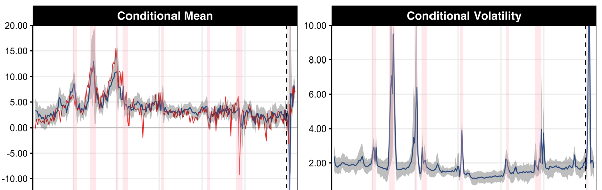
(a) Full Sample

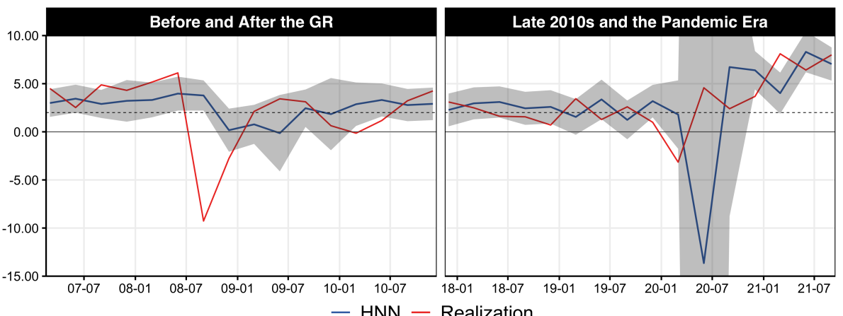
(b) Zooming on Particular Episodes

Figure 10: Results for benchmark HNN-F specification with evolving volatility, with training ending in 2019Q4. In the first panel, the dashed line is the beginning of the out-of-sample. In the second, it is the 2% inflation target. The Conditional Volatility plot is limited above at 10 for visibility. Gray bands around the predictions are $\pm 1\enskip h_{t,v}$ as estimated by HNN. Gray bands around $h_{t,v}$ is the usual 68% credible region obtained from the bootstrap.

Figure 10 reports results from HNN-F with evolving volatility. The resulting $h_{t,v}$ showcase diverse kinds of fluctuations. First, we get volatility blasts during all recessions punctuated with important fluctuations in the price of oil. This is something that a SV model based on the random walk – hence putting the accent on longer-run changes – would hardly capture. The various plots of Figure 10 have a capped y-axis because, as one could expect, the out-of-sample volatility forecast skyrockets following the first 2020 economic shutdown. In accord with most SV estimations, we get a significant decline in the volatility level at "rest" during the Great Moderation. Volatility in the last decade has been comparable to that of non-recession periods of the 1970s. It appears that the most appropriate "classical" specification of the volatility process would be a 2- or 3-state switching process based on observables, combined with a slow-moving component. Conveniently, this augmented HNN-F had learned those patterns nonparametrically using data through 2019Q4.

The highest pre-pandemic volatility peaks – the two inflation spirals of the 1970s – are topped by a huge margin for the 2020Q3 and 2020Q4 forecasts. As is clearly visible in the second panel of Figure 10(b), HNN-F knows its forecasts are highly uncertain following the unprecedented variations in macroeconomic indicators. In fact, the bands simply reveal that the network, being handed only macroeconomic data and no additional information, sees everything as possible. This is not surprising given how reliant on extrapolations such forecasts are — many inputs exited their usual range with an unprecedented vigor. HNN completely comes back to its senses in 2021Q1 and appears confident in its forecasts, whose $\pm 1\enskip h_{t,v}$ bands effectively exclude the inflation target. In terms of the quality of point forecasts, those reported in 10(a) are comparable to those of Figure 7(b) for the most part. However, while plain HNN-F predictions in Figure 7(b) are slightly below the late 2021 realizations, the above version including the volatility hemisphere produces well-centered forecasts for the tumultuous period.

From an econometric point of view, it appears that this "augmented" HNN can aptly predict the likelihood of its own demise. This is a highly desirable feature. While providing a strikingly erroneous forecast for 2020Q3 in Figure 7(b), it communicated its user that, based on historical patterns, this particular forecast is extremely uncertain. This further motivates the exclusion of 2020 observations in the barplots of Figure 7 – and based on estimation set in stone in 2019Q4. Observing the disturbing volatility predictions, a user would look for modeling alternatives such as heuristic forecasts. In Figure 10(b), we see a similar (yet much more moderate) pattern for the 2008 recession and its aftermath. That is, forecasts are too low for first two quarters of 2009, but the bands widen in a timely manner to include the realized values.

This section is merely a first step in the direction of time-varying uncertainty prediction within a single network. Its purpose is to show that yes, HNN can conveniently and flexibly model inflation volatility while retaining its original advantages.

6 HNN as an Evaluator or Generator of New Theories

With typical PC regressions often being only mildly supported by the data, there has been a business of proposing augmented PCs. Often times, the newly proposed component is either suggested from formal theory or common sense economic arguments. In both cases, there can be a disconnect between what is in the database and what comes out of the theory, again compromising the proper evaluation of the potency of such augmentations. By adding new hemispheres dedicated to the newcomers, HNN can palliate this problem.

6.1 An Investigation of the 4-Equation NK Model

sims2019four introduce a four-equation New Keynesian model that skillfully blends the tractability (and the derivation of an explicit Phillips curve) of the canonical 3-equation model (gali2015monetary) and relevance for analyzing the effects of quantitative easing (QE). As a result of incorporating, among other things, financial intermediaries, bonds of different terms, and credit market shocks, their Phillips curve includes two additional variables beyond those of (1): the real market value of the monetary authority’s long-term bond portfolio and credit conditions. While the former is rather clearly defined in terms of observed variables, the latter needs to be proxied, and ambiguity reigns as to which financial market variable will adequately proxy for "credit conditions". The HNN solution is now obvious: create a $\mathcal{H}$ with a myriad of indicators containing information on the health of credit markets.

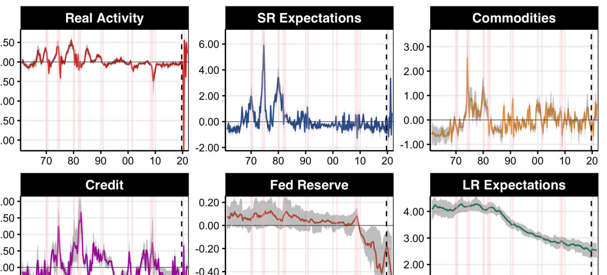
Figure 11: Contributions ($h_{t}$’s) from HNN-F-4NK. Notes: Dashed line is the beginning of the out-of-sample. NBER recessions are in pink shadowing. Gray shading is the 68% credible region.

The expected signs for coefficients, as derived from theory, is that keeping the output gap fixed, favorable credit conditions bring inflation downward, and so does an expanding positive central bank balance sheet. Those signs are obviously those of marginal effects, i.e., when controlling for the output gap. In this section, I augment HNN-F with two additional hemispheres inspired from sims2019four’s model. Then, results regarding the effect of credit conditions are compared to a much simpler model – a PC regression with time-varying parameters that is augmented with oil prices, the reserves of depository institutions (total and non-borrowed), and, most importantly, the Chicago Fed National Financial Conditions Credit Subindex.

Figure 11 reports, among other things, the contribution of credit conditions and the Fed expanding balance sheet to $\pi_{t+1}$ as estimated from HNN-F. The four original components are largely unchanged, largely because the additional two are of limited relative importance. Figure 12 reports results from augmented PC regressions with time-varying parameters. The NFCI is found to have a negligible impact on $\pi_{t+1}$, whereas the credit index created endogenously by HNN-F from the credit group of variables in FRED-QD (see mccracken2020fred for the complete list) has an appreciable effect during certain historical episodes. For instance, there is mild upward pressure on prices due to tightening credit conditions before and after the early 1990s recession, as well in running up to the GR. Also, loose credit conditions and an ever-expanding Fed balance sheet are credited for very light (direct, not indirectly through the gap) downward pressure on prices during the mid 2010s. This is, obviously, the direct marginal effect, keeping the gap fixed.

In Figure 12, the HNN credit conditions index shares some peaks and troughs with NFCI-Credit and mostly overall NFCI, but, all in all, they are only mildly correlated. As a result, compared to a more traditional test of the 4-NK model, we get a much larger (and correctly signed) coefficient for credit conditions in HNN. This is explained by HNN’s index being active during certain periods while either NFCI-Credit is essentially flat (from the early 1980s on, excluding the GR) or has the opposite sign (for almost all of the 1970s). Thus, unlike classical methods, HNN finds a mild positive contribution of tightening credit conditions from the mid 1980s until the early 1990s, an era punctuated by the 1987 stock market crash and a general credit slowdown from 1989-1992 (akhtar1994causes). Additionally, HNN finds easy credit conditions from 1995 until 2005, with the exception of a small peak following the collapse of the Dotcom bubble. Overall, the credit conditions index created by "inflation supervision" is suggestive of a much less persistent behavior and much more action during the Great Moderation than what can be seen from the NFCI-Credit. Finally, the coefficient on credit index is found to be declining exogenously through time starting from 1980s but then experience a revival in the 2010s. However, there is wide uncertainty surrounding the coefficient estimates of the last decade.

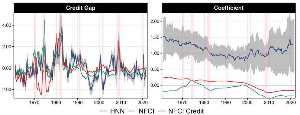
Figure 12: HNN-F-4NK’s "credit conditions" and associated time-varying coefficient. Notes: Dashed line is the beginning of the out-of-sample. NBER recessions are in pink shadowing. Gray shading is the 68% credible region. NFCI indices prior to 1971 are patched using SW2002’s EM algorithm applied on the whole FRED-QD dataset. Coefficients for the last two specifications are obtained from time-varying parameter PC regressions (see Figure 3 notes for details)) augmented with the Fed’s balance sheet each credit conditions index in turns .

From a methodological standpoint, the takeaway message is the following. If one chooses the NFCI-Credit, arguably a very legitimate proxy for credit conditions as they enter sims2019four’s PC, literally no empirical support is found for the new model. In contrast, HNN, by constructing a credit index supervised by $\pi_{t+1}$, finds some evidence for the PC as derived by sims2019four. This contribution of credit conditions – albeit light when compared to that of the original four components – is nontrivial. The same cannot be said of the Fed’s reserves, which have a limited direct effect on $\pi_{t+1}$. But this could be due to the limited length of the "QE sample".

6.2 Adding an International Component and a Kitchen Sink

The connectedness of the world economy suggests inflation can be influenced by non-domestic factors, like the vigor of the trading partners’ economy. There is cross-sectional and time series evidence on the matter (borio2007globalisation; laseen2016did; bobeica2019missing) and it is not infrequent to see proxies of international economic or inflation conditions enter PC regressions (blanchard2015inflation). The 2021 inflation experience, with many countries reporting historically high YoY inflation rates simultaneously, does not negate the importance of a global component either. As always, the question is how to properly construct a global measure of slack that may or may not influence US inflation, when controlling for its own gap.

To create a global gap (excluding the US), I construct a hemisphere where the inputs are quarterly GDP growth rates from 1970 for OECD members and potential member states, which data is available here. Country aggregations (like G7, to avoid overlap with domestic variables) are excluded, and so are countries which data starts post-1960.

Since this specification is not motivated from any tight theory (as it was the case in Section 6.1), I also indulge in adding a Kitchen Sink hemisphere, which, as the name suggests, will include all the variables in FRED-QD that are not already included in our four benchmark hemispheres. This will provide yet another robustness check on the path estimated for key components like $g_{t}$ and ${\mathcal{E}_{t}^{\text{SR}}}$. This can also point, via the VI analysis, to variables that could eventually deserve their own hemispheres in extensions of this work. The resulting specification is referred to as HNN-F-IKS, namely, HNN-F with an international component and a kitchen sink.

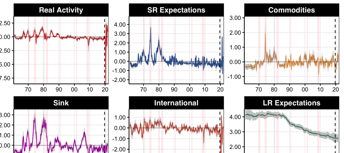
Figure 13: Contributions ($h_{t}$’s) from HNN-F-IKS. Notes: Dashed line is the beginning of the out-of-sample. NBER recessions are in pink shadowing. Gray shading is the 68% credible region.

The international output gap seems to be of limited importance compared to other components — its contribution is typically contained within the -0.5 to 0.5 range and the bands often times includes 0. This statement, of course, does not apply to the Pandemic era where massive swings similar to those of $g_{t}$ are observed. Notable recent episodes are a flash negative contribution circa the GR and a gently negative one in the mid-2010s, corresponding to the missing inflation period.

In Figure 13, it is found that $g_{t}$ and ${\mathcal{E}_{t}^{\text{SR}}}$ are qualitatively unchanged, but one can notice an overall weakened effect (with respect to Figure 2) of both components especially in the 1970s. The major reason for that last observation is arguably the commanding presence of the kitchen sink, which contribution entertain some important highs in the 1970s, as well as three intriguing bumps before the 1990, 2001, and 2008 recessions. Importantly, it is worth remembering that its very inclusion changes the definition of $g_{t}$ and ${\mathcal{E}_{t}^{\text{SR}}}$ are per the network structure. Thus, their reported dampening should be taken with a grain of salt.

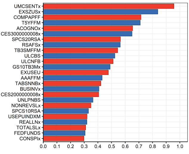
Figure 14: VI Results for the Kitchen Sink component of HNN-F-IKS specification, with training ending in 2019Q4. Mnemonics are those of FRED-QD.

Nonetheless, understanding what is in the sink could clearly prove valuable. Figure 14, by reporting the VI for the sink component, strongly suggests that information about future economic outcomes is key: the first six variables are all considered leading indicators. Very interestingly, it is, again, the survey variant of such expectations that comes on top (UMCSENTx). Then, comes market-based forward-looking variables: a US exchange rate followed by three spreads (5-year treasury bill minus federal fund rate (FFR), 3-month commercial paper minus FFR, 3-month treasury bill minus FFR). The literature documenting the potency of spreads as predictors of business cycle turning points is vast (stock1989new; estrella1998predicting). Their link to inflation seems thinner (stock2008phillips) in linear PC regressions but MRF finds that their link to inflation appears to be highly nonlinear (using a newly developed random forest approach). HNN also can deal with the necessary nonlinearities.

Finally, SPCS20RSA (S&P/Case-Shiller 20-City Composite Home Price Index) and ACOGNOx (Manufacturers’ New Orders for Consumer Goods Industries) are both leading indicators within their own economic sectors. Overall, there is a clear push from forward-looking variables during the periods that precede economic downturns. This large weight accorded to variables inputting information about future economic outcomes is not surprising, as the latter is directly related to expectations about future marginal costs (and so are unit labor costs, entering at positions 10 and 11 in Figure 14) – solving forward the NKPC yields that $\pi_{t}$ is a function of expected future marginal costs. The empirical importance of considering forward-looking expectations about the marginal costs has been highlighted before, mostly from a structural model perspective (del2015inflation). Nonetheless, it is worth remembering that VI results for the kitchen sink are more dispersed than those of Figure 8 and it is clear that a plethora of regressors contribute to the component beyond those at the top.

7 Parting Words

This paper estimates a neural Phillips Curve with a deep output gap by developing the Hemisphere Neural Network. Results vary substantially from those obtained with traditional econometric methods by dispensing with a plethora of assumptions inherent to the latter. Among others: the choice of variable from which the gap should be made of, filter choices and laws of motions, restrictive time variation in coefficients, etc. As a result, unlike time-varying PC regressions with the CBO gap or others, HNNs delivers good forecasts, like capturing some of the upswing in the CPI observed in 2021. The model attributes some of it to a widening positive output gap, unlike traditional estimates which typically deliver negative (or mildly positive) gaps throughout 2021. Additionally, unlike methodologies which impose smoothness assumptions through autoregressive laws of motion, HNN’s gap is highly volatile during the Pandemic period – a finding consistent with the intermittent closing/opening of the economy following the successive waves of Coronavirus infections.

It is shown that the HNN framework can be extended in many directions. One is to test more sophisticated Phillips Curve specifications by creating hemispheres for theoretical additions that are not well defined in terms of actual variables. Another is to predict inflation volatility directly within the same model without any significant alteration to the code or computations.

From a general econometric standpoint, this work calls into question the quasi-hegemony of filtering methods when it comes to latent states extraction in macroeconomics. In fact, it appears that alternative routes leveraging larger databases, modern machine learning techniques, and cutting-edge computing environments can contribute to economic debates in ways their predecessors could not.

Appendix A Appendix

A.1 Additional Figures

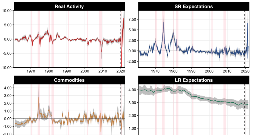
Figure 15: Contributions ($h_{t}$’s) from HNN. Notes: Dashed line is the beginning of the out-of-sample. NBER recessions are in pink shadowing.

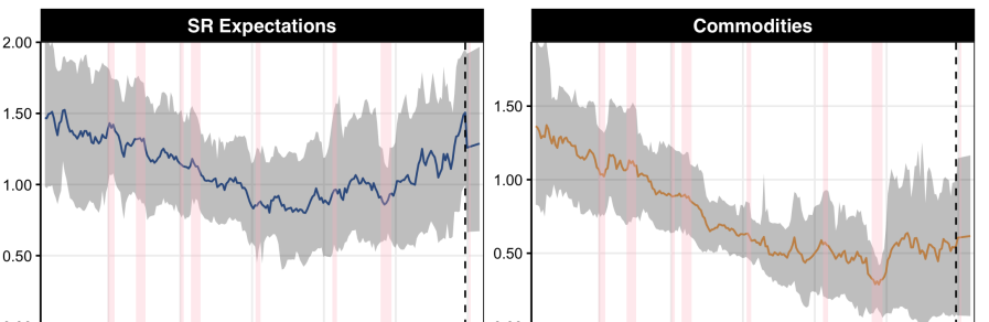
Figure 17: HNN-F’s remaining two time-varying coefficients. Notes: Dashed line is the beginning of the out-of-sample. NBER recessions are in pink shadowing. Grey shading is the 68% credible region.

A.2 Ablation Studies

HNN involves many ingredients, like the use of many economic indicators and nonlinear supervised processing. In this section, I conduct a brief inspection of what happens when dispensing with one or the other.

Table 2: Data-Poor $\mathcal{H}$’s

$\mathcal{H}$	Content
$\mathcal{E}_{t}^{\text{LR}}$	$t$ (exogenous time trend)
$\mathcal{E}_{t}^{\text{SR}}$	Inflation expectations from SPF, and Michigan Survey, lags of $\pi_{t}$, $t$
$g_{t}$	Unemployment, $t$
$c_{t}$	Oil price, $t$

First, I consider a specification where key hemispheres only contains what would enter in typical modern PC OLS-based regression, as detailed in Table 2. Essentially, more fine-grained data on prices and any real activity indicator except for unemployment have been liquidated (with respect to Table 1). Unemployment is now in levels and aforementioned transformations (lags and moving averages) are kept. The idea is to have the neural network filter unemployment itself by nonlinearly interacting it with $t$, analogously to what unsupervised filtering does. In this context, for identification reasons (detrending unemployment and estimating a trending coefficient on it), HNN (not HNN-F) results are reported in Figure 19 and the focus is kept on contributions.

Here are key observations from Figure 19. The contribution of real activity is much smaller in absolute terms throughout the sample than it it is for baseline specifications, highlighting the importance of diversified real activity indicators. The bands include 0 much more often starting from the 2000s, in line with traditional results using filtered unemployment. Speaking of, the extracted $h_{t,g}$ looks much more like filtered unemployment, albeit smaller $\lambda$ (Hodrick-Prescott smoothing parameter) than what is typically used. Lastly, and rather not unexpectedly, $h_{t,g}$ is negative all Pandemic long (as of 2021Q3) making it rather unequipped to force its inflation forecast upward during the last 3 quarters. All in all, the inclusion of many real indicators in $\mathcal{H}_{g}$ seems vital for a more proactive characterization of real activity. This is not an unfamiliar conclusion (SW2002).

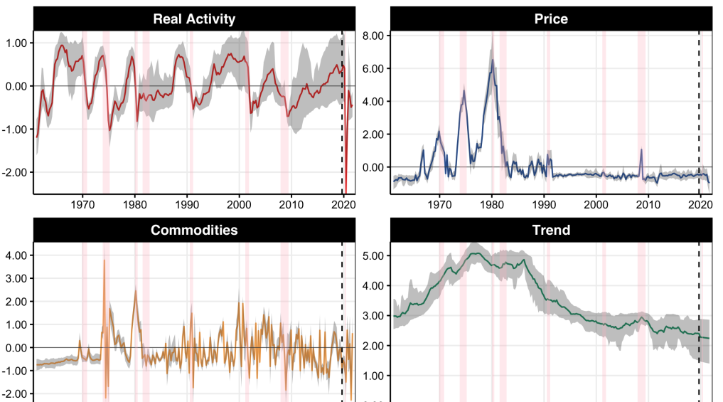
Figure 19: A Look at HNN components ($h_{t}$’s) with limited data in hemispheres. Notes: Dashed line is the beginning of the out-of-sample. NBER recessions are in pink shadowing.

The expectations component is more alike what reported throughout the paper (e.g., Figures 2 and 15). This is not surprising given the high importance accorded to survey expectations and lags of the CPI by HNN, as reported by VI calculations in Figure 8(b). However, in 19 their nonlinear processing is even more evident: the component is drastically shut down starting from 1990, and only wakes up for one obvious spike during the Great Recession. The contribution, however, excludes the 2021Q2 very noticeable peak, which makes the forecast takes off (Figure 4(b)) from the historical mean. Thus, dispensing with the vast number of price series originally included in HNN leads to missing key abrupt changes in the short-run expectations component that go under the radar of traditional aggregated measures.

The second ablation study exercise maintain the data-rich environment, but dispense with nonlinearities and supervision (in part). Figure 20 conducts different PCA-based extractions of the data contained in $\mathcal{H}_{g}$ and $\mathcal{H}_{\mathcal{E}^{\text{SR}}}$. A few alternatives are reported. PCA Real Activity means reporting the first factor of $\mathcal{H}_{g}$. Weighted PCA Real Activity means that, after standardization, variables were given weights in accord to VI estimates from Figure 8. This brings back some of the supervision from HNN. The real activity part of Figure 20 contains two additional extractions. PCA All is the first factor of all the contemporaneous data included in HNN, whereas PCA All+ includes lags and MARX’s as well. The rationale for including the last two (in the top part of the panel only) stems from the often reported finding that the first factor extracted from broad macroeconomic panels looks very much like a real activity factor (mccracken2020fred).

Findings are as follows. In Figure 20(a), PCA extractions, except for the weighted version, form a cluster throughout. For the period spanning from 2000 to the Pandemic era, that cluster seemingly includes $g_{t}^{\text{HNN}}$. However, during periods of overheating, differences are manifest and no linear method seem to approximate $g_{t}^{\text{HNN}}$. This is true of the 1970s, and also of the current period (Figure 20(b))), with two linear extractions signaling no overheating at all, and two others showing a rather quaint or short-lived one. Weighted PCA Real Activity is mostly far away $g_{t}^{\text{HNN}}$ from the pack, suggesting nonlinear processing of important variables (such as the Help-Wanted Index, which trend is clearly visible in Weighted PCA Real Activity) cannot be dispensed with. Nevertheless, this "mildly supervised" PCA extraction is the only one pointing to a widening positive gap in 2021 – as does $g_{t}^{\text{HNN}}$.

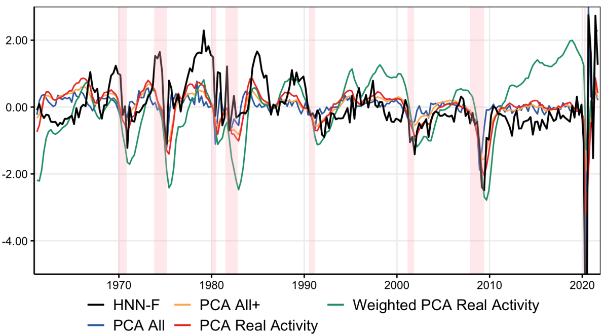
(a) Alternative Data-Rich $g_{t}$ Extraction

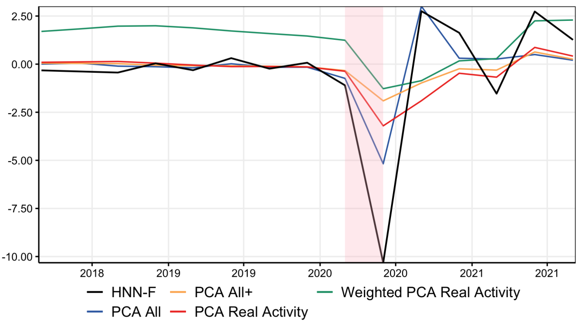
(b) Alternative Data-Rich $g_{t}$ Extraction – Last 3 years

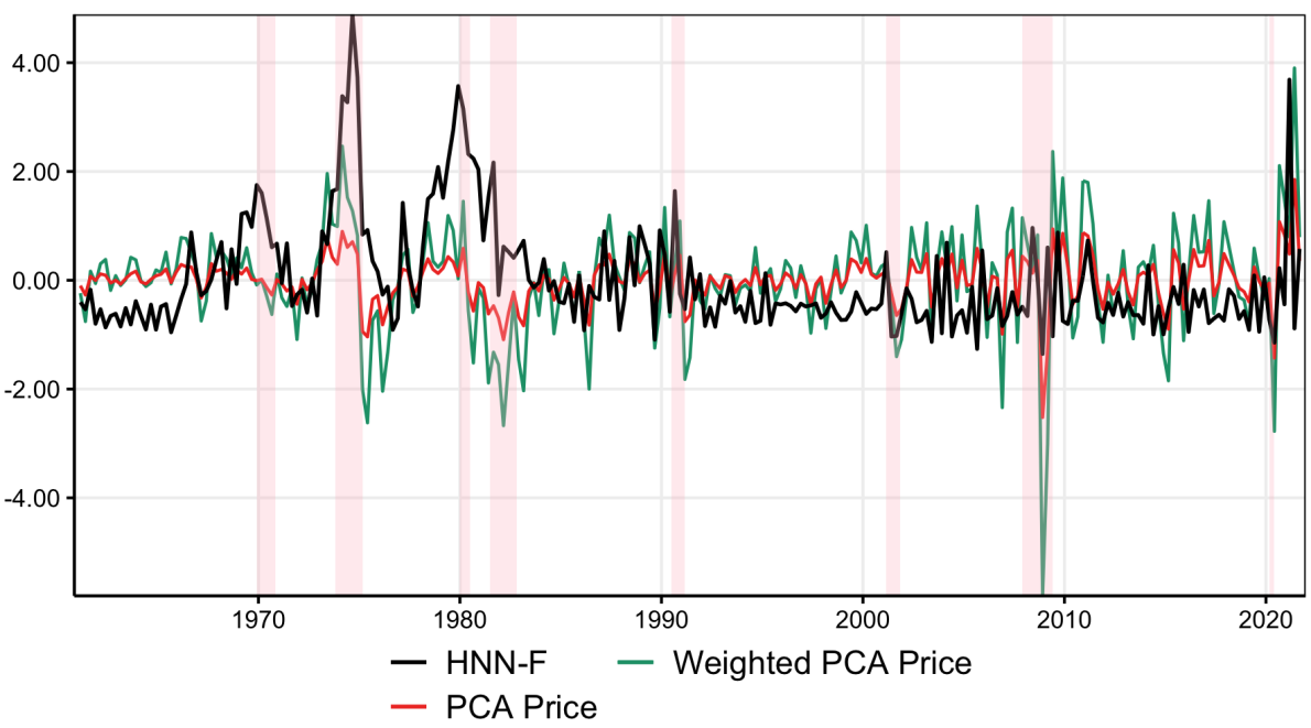
(c) Alternative Data-Rich $\mathcal{E}_{t}^{\text{SR}}$ Extraction

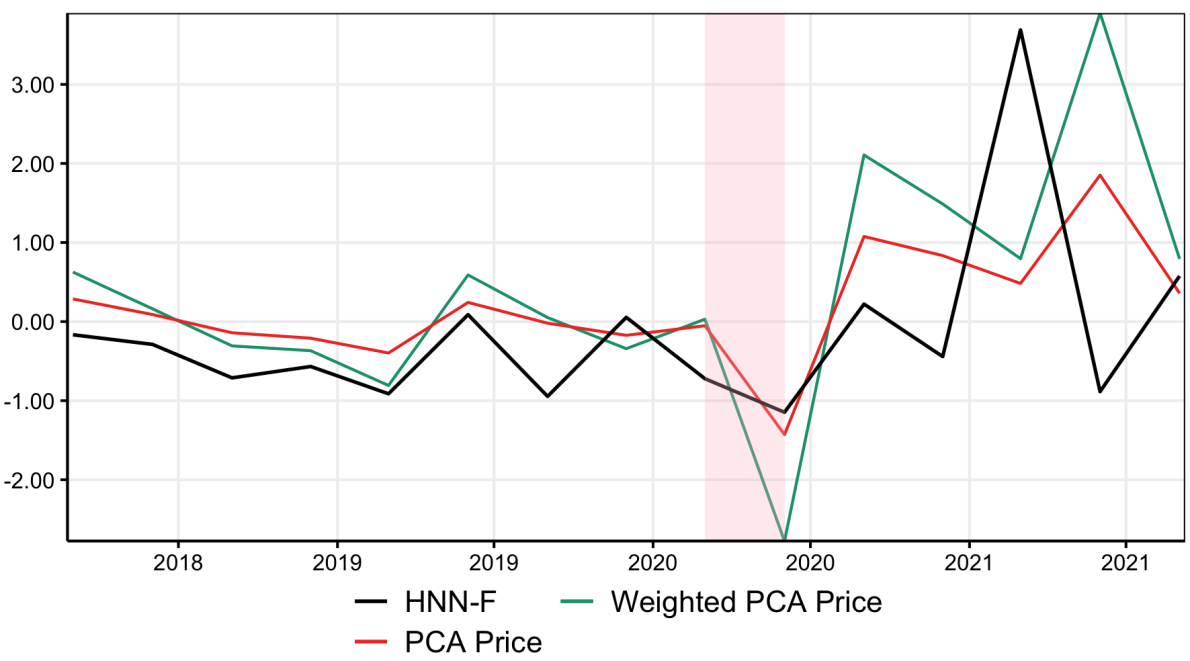
(d) Alternative Data-Rich $\mathcal{E}_{t}^{\text{SR}}$ Extraction – Last 3 years

Figure 20: "Gaps" of the four $\mathcal{H}$’s through time according to different extraction techniques. Notes: all NN estimations end in 2019 and are projected out-of-sample from there. Pink shading is NBER recessions.

Differences between PCA extracts and HNN-F’s own $\mathcal{E}^{\text{SR}}$ are very apparent in Figure 20(c). For instance, HNN-F’s $\mathcal{E}^{\text{SR}}$ essentially consists in being resting around 0 or having important positive peaks – i.e., there is no important downward pressure from expectations as suggested by either PCA or its weighted version (for instance 2008, or after the 2nd 1980s recession). Obviously, the non-symmetrical behavior of $\mathcal{E}^{\text{SR}}$ is possible due to nonlinear processing through the network. This behavior is also noticeable in Figure 20(d), with PCA and the mildly supervised PCA mostly being indicators of current inflation, whereas $\mathcal{E}^{\text{SR}}$ does not dip following the flash recession (like prices themselves), but exhibit an abrupt peak a few quarters later. Thus, nonparametric nonlinear processing seems to be vital in extracting $\mathcal{E}^{\text{SR}}$ from price and expectations data that is actually forward-looking.

Overall, results from the Ablation studies suggest that both using vast amounts of data and nonlinear supervised processing of it are essential to obtain the desirable $g_{t}$ and $\mathcal{E}^{\text{SR}}$ delivered by HNN-F.

A.3 Taylor Rule Supervision

This section explores a curiosity which can be understood as a more radical change of supervisors than what reported in Section 4.3. From an econometric point of view, it showcases yet one of the many potential applications of HNN beyond inflation and Phillips curves.

Inflation is retired in favor of the federal funds rate and the supervision relationship becomes an empirical Taylor rule. That is, we are extracting the contribution of the gap and inflation to the monetary policy instrument values. An interesting economic question is whether $h_{t,g}^{\text{FFR}}$ looks remotely like $h_{t,g}^{\text{CPI}}$. In other words, does the "fed view" of the gap – assuming the Taylor rule is a valid approximation to its behavior – coincides with what the inflation record suggests?

There are two important changes with respect to the baseline specification. First, $\pi_{t+1}$ is replaced by the federal fund rate next period ($r_{t+1}$). Second, the energy/commodities group is replaced by the "Smoothing" group which includes lags of $r_{t+1}$. This inclusion is typical of empirical Taylor rules and statistically accommodates for the fact that the monetary authority avoids drastic changes in $r_{t}$.

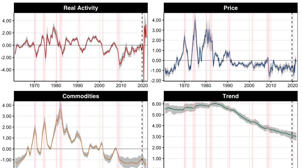
Figure 21: Contributions ($h_{t}$’s) based on a Taylor Rule, with training ending in 2019. Notes: Dashed line is the beginning of the out-of-sample. NBER recessions are in pink shadowing.

In Figure 21, $h_{t,g}^{\text{FFR}}$ looks much more like what one would obtain from traditional filtering-based gap except for the Pandemic episode. First, there is a certain persistence to it that is characteristic of specification assuming autoregressive laws of motion. Second, albeit remaining cyclical, the contribution is mostly negative starting from the 2000s, whereas it was roughly symmetrical around 0 beforehand – which is reminiscent of many unemployment-related measures of slack (stock2019slack). Third, it mostly exhibits a slow climb back to 0 starting from 2008, like one would obtain from, e.g., the CBO gap.

There are 3 episodes where predictions (unreported) from this model can be off for a few quarters. First, the two ZLB episodes, where this Taylor rule prescribes interest rates going below zero—not inconsistent with the deployment of quantitative easing following the GR and during the Pandemic period. Interestingly, the third episode is right now, with $h_{t,g}^{\text{FFR}}$ asking for much higher rates than those currently in effect. In other words, if the Fed was consistent with how it responded to slack/overheating (as extracted by HNN-F) during the last decades, rates should be higher than they are right now. Two grains of salt on this statement are that (i) the Fed changed its approach to inflation targeting in 2020, and (ii) Pandemic era slack is different from previous recessions slack (like the distributive aspects of it) and addressing it more upfront will have different (likely higher) costs on other dimensions of economic well-being. A formalization of this view is that, in times of sectoral (or structural) reallocation, the divine coincidence is broken, leading to an "optimal" level of inflation that is above the target (guerrieri2021monetary). However, an important drawback of deviating from the HNN-based Taylor Rule is the risk of disanchoring expectations—which for now appears mild since economic agents can allegedly differentiate between what one should expect from normal and Pandemic economic times.

The evident wedge between $h_{t,g}^{\text{FFR}}$ and $h_{t,g}^{\text{CPI}}$ reported throughout the paper hints that there may be a gap between the monetary authority’s view of economic slack and what matches the inflation record. Nonetheless, this application is meant as illustrative about HNN versatility, and to understand further how supervision affect $g_{t}$. A comprehensive assessment of "neural Taylor rules" is material for future work.

A.4 Mnemonics for Benchmark HNNs

⬇

#These are for HNN-F. Add "trend" to the first three hemispheres to get HNN.

real.activity.hemisphere <- c("PAYEMS","USPRIV","MANEMP","SRVPRD",

"USGOOD" ,"DMANEMP","NDMANEMP","USCONS","USEHS",

"USFIRE","USINFO","USPBS","USLAH","USSERV",

"USMINE","USTPU","USGOVT","USTRADE",

"USWTRADE","CES9091000001","CES9092000001",

"CES9093000001","CE16OV","CIVPART",

"UNRATE","UNRATESTx","UNRATELTx","LNS14000012",

"LNS14000025","LNS14000026",

"UEMPLT5","UEMP5TO14","UEMP15T26","UEMP27OV",

"LNS13023621","LNS13023557",

"LNS13023705","LNS13023569","LNS12032194",

"HOABS","HOAMS","HOANBS","AWHMAN",

"AWHNONAG","AWOTMAN","HWIx","UEMPMEAN",

"CES0600000007", "HWIURATIOx","CLAIMSx","GDPC1",

"PCECC96","GPDIC1","OUTNFB","OUTBS","OUTMS",

"INDPRO","IPFINAL","IPCONGD","IPMAT","IPDMAT",

"IPNMAT","IPDCONGD","IPB51110SQ","IPNCONGD",

"IPBUSEQ","IPB51220SQ","TCU","CUMFNS",

"IPMANSICS","IPB51222S","IPFUELS")

SR.expec.hemisphere <- c("Y", "PCECTPI","PCEPILFE",

"GDPCTPI","GPDICTPI","IPDBS", "CPILFESL","CPIAPPSL",

"CPITRNSL","CPIMEDSL","CUSR0000SAC","CUSR0000SAD",

"WPSFD49207", "PPIACO","WPSFD49502","WPSFD4111",

"PPIIDC","WPSID61","WPSID62","CUSR0000SAS","CPIULFSL",

"CUSR0000SA0L2","CUSR0000SA0L5", "CUSR0000SEHC",

"spf_cpih1","spf_cpi_currentYrs","inf_mich")

commodities.hemisphere <- c("WPU0531","WPU0561","OILPRICEx","PPICMM")

LR.expec.hemisphere <- c("trend")

credit.hemisphere <- c("BUSLOANSx","CONSUMERx","NONREVSLx",

"REALLNx","REVOLSLx","TOTALSLx","DRIWCIL", "DTCOLNVHFNM",

"DTCTHFNM","INVEST","nfci","nfci_credit","nfci_nonfin")

References

- Adrian et al., (2019) Adrian, T., Boyarchenko, N., and Giannone, D. (2019). Vulnerable growth. American Economic Review, 109(4):1263–89.
- Agarwal et al., (2020) Agarwal, R., Frosst, N., Zhang, X., Caruana, R., and Hinton, G. E. (2020). Neural additive models: Interpretable machine learning with neural nets. arXiv preprint arXiv:2004.13912.
- Akhtar et al., (1994) Akhtar, M. et al. (1994). Causes and consequences of the 1989-92 credit slowdown: overview and perspective. Studies on Causes and Consequences of the 1989-92 Credit Slowdown, Federal Reserve Bank of New York, pages 1–38.
- Almosova and Andresen, (2019) Almosova, A. and Andresen, N. (2019). Nonlinear inflation forecasting with recurrent neural networks. May 2019.
- Andreini et al., (2020) Andreini, P., Izzo, C., and Ricco, G. (2020). Deep dynamic factor models. arXiv preprint arXiv:2007.11887.
- Atkeson and Ohanian, (2001) Atkeson, A. and Ohanian, L. E. (2001). Are phillips curves useful for forecasting inflation? Federal Reserve bank of Minneapolis quarterly review, 25(1):2–11.
- Ball and Mazumder, (2019) Ball, L. M. and Mazumder, S. (2019). The nonpuzzling behavior of median inflation. Technical report, National Bureau of Economic Research.
- Banbura and Bobeica, (2020) Banbura, M. and Bobeica, E. (2020). Does the phillips curve help to forecast euro area inflation?
- Banbura et al., (2021) Banbura, M., Leiva-Leon, D., and Menz, J.-O. (2021). Do inflation expectations improve model-based inflation forecasts?
- Barigozzi and Luciani, (2018) Barigozzi, M. and Luciani, M. (2018). Measuring us aggregate output and output gap using large datasets. Technical report, Working paper.
- Barkan et al., (2020) Barkan, O., Caspi, I., Hammer, A., and Koenigstein, N. (2020). Predicting disaggregated cpi inflation components via hierarchical recurrent neural networks. arXiv preprint arXiv:2011.07920.
- Barnichon, (2010) Barnichon, R. (2010). Building a composite help-wanted index. Economics Letters, 109(3):175–178.
- Bartlett et al., (2020) Bartlett, P. L., Long, P. M., Lugosi, G., and Tsigler, A. (2020). Benign overfitting in linear regression. Proceedings of the National Academy of Sciences.
- Belkin et al., (2019) Belkin, M., Hsu, D., Ma, S., and Mandal, S. (2019). Reconciling modern machine-learning practice and the classical bias–variance trade-off. Proceedings of the National Academy of Sciences, 116(32):15849–15854.
- Bender et al., (2020) Bender, G., Liu, H., Chen, B., Chu, G., Cheng, S., Kindermans, P.-J., and Le, Q. V. (2020). Can weight sharing outperform random architecture search? an investigation with tunas. In Proceedings of the IEEE/CVF Conference on Computer Vision and Pattern Recognition, pages 14323–14332.
- Berger et al., (2021) Berger, T., Boll, P. D., Morley, J., and Wong, B. (2021). Cyclical signals from the labor market.
- Berger et al., (2020) Berger, T., Morley, J., and Wong, B. (2020). Nowcasting the output gap. Journal of Econometrics.
- Binder, (2015) Binder, C. C. (2015). Whose expectations augment the phillips curve? Economics Letters, 136:35–38.
- Blanchard, (2016) Blanchard, O. (2016). The phillips curve: Back to the’60s? American Economic Review, 106(5):31–34.
- Blanchard, (2021) Blanchard, O. (2021). In defense of concerns over the $1.9 trillion relief plan. Peterson Institute for International Economics Realtime Economic Issues Watch, 18.
- Blanchard et al., (2015) Blanchard, O., Cerutti, E., and Summers, L. (2015). Inflation and activity–two explorations and their monetary policy implications. Technical report, National Bureau of Economic Research.
- Bobeica and Jarociński, (2019) Bobeica, E. and Jarociński, M. (2019). Missing disinflation and missing inflation: A var perspective. 57th issue (March 2019) of the International Journal of Central Banking.
- Borio and Filardo, (2007) Borio, C. E. and Filardo, A. J. (2007). Globalisation and inflation: New cross-country evidence on the global determinants of domestic inflation.
- Borup et al., (2020) Borup, D., Rapach, D., and Schütte, E. C. M. (2020). Now-and backcasting initial claims with high-dimensional daily internet search-volume data. Available at SSRN 3690832.
- Breiman, (1996) Breiman, L. (1996). Bagging predictors. Machine learning, 24(2):123–140.
- Breiman, (2001) Breiman, L. (2001). Random forests. Machine learning, 45(1):5–32.
- Bulligan et al., (2019) Bulligan, G., Guglielminetti, E., and Viviano, E. (2019). Adjustments along the intensive margin and wages: Evidence from the euro area and the us.
- Carriero et al., (2021) Carriero, A., Clark, T. E., Marcellino, M. G., and Mertens, E. (2021). Addressing covid-19 outliers in bvars with stochastic volatility.
- Chan et al., (2018) Chan, J. C., Clark, T. E., and Koop, G. (2018). A new model of inflation, trend inflation, and long-run inflation expectations. Journal of Money, Credit and Banking, 50(1):5–53.
- Chan et al., (2016) Chan, J. C., Koop, G., and Potter, S. M. (2016). A bounded model of time variation in trend inflation, nairu and the phillips curve. Journal of Applied Econometrics, 31(3):551–565.
- Choudhary and Haider, (2012) Choudhary, M. A. and Haider, A. (2012). Neural network models for inflation forecasting: an appraisal. Applied Economics, 44(20):2631–2635.
- Clyde and Lee, (2001) Clyde, M. and Lee, H. (2001). Bagging and the bayesian bootstrap. In AISTATS.
- Coibion and Gorodnichenko, (2015) Coibion, O. and Gorodnichenko, Y. (2015). Is the phillips curve alive and well after all? inflation expectations and the missing disinflation. American Economic Journal: Macroeconomics, 7(1):197–232.
- Coibion et al., (2018) Coibion, O., Gorodnichenko, Y., and Kamdar, R. (2018). The formation of expectations, inflation, and the phillips curve. Journal of Economic Literature, 56(4):1447–91.
- De Carvalho and Rua, (2017) De Carvalho, M. and Rua, A. (2017). Real-time nowcasting the us output gap: Singular spectrum analysis at work. International Journal of Forecasting, 33(1):185–198.
- Del Negro et al., (2015) Del Negro, M., Giannoni, M. P., and Schorfheide, F. (2015). Inflation in the great recession and new keynesian models. American Economic Journal: Macroeconomics, 7(1):168–96.
- Del Negro et al., (2020) Del Negro, M., Lenza, M., Primiceri, G. E., and Tambalotti, A. (2020). What’s up with the phillips curve? Technical report, National Bureau of Economic Research.
- Dufour et al., (2006) Dufour, J.-M., Khalaf, L., and Kichian, M. (2006). Inflation dynamics and the new keynesian phillips curve: an identification robust econometric analysis. Journal of Economic dynamics and control, 30(9-10):1707–1727.
- Durbin and Koopman, (2012) Durbin, J. and Koopman, S. J. (2012). Time series analysis by state space methods. Oxford university press.
- d’Ascoli et al., (2020) d’Ascoli, S., Refinetti, M., Biroli, G., and Krzakala, F. (2020). Double trouble in double descent: Bias and variance (s) in the lazy regime. In International Conference on Machine Learning, pages 2280–2290. PMLR.
- Engle, (1982) Engle, R. F. (1982). Autoregressive conditional heteroscedasticity with estimates of the variance of united kingdom inflation. Econometrica: Journal of the econometric society, pages 987–1007.
- Estrella and Mishkin, (1998) Estrella, A. and Mishkin, F. S. (1998). Predicting us recessions: Financial variables as leading indicators. Review of Economics and Statistics, 80(1):45–61.
- Farrell et al., (2021) Farrell, M. H., Liang, T., and Misra, S. (2021). Deep neural networks for estimation and inference. Econometrica, 89(1):181–213.
- Faust and Wright, (2013) Faust, J. and Wright, J. H. (2013). Forecasting inflation. In Handbook of economic forecasting, volume 2, pages 2–56. Elsevier.
- Forbes et al., (2021) Forbes, K., Gagnon, J., and Collins, C. G. (2021). Low inflation bends the phillips curve around the world. Technical report, National Bureau of Economic Research.
- Friedman et al., (2001) Friedman, J., Hastie, T., and Tibshirani, R. (2001). The elements of statistical learning, volume 1. Springer series in statistics New York, NY, USA:.
- Friedman, (2001) Friedman, J. H. (2001). Greedy function approximation: a gradient boosting machine. Annals of statistics, pages 1189–1232.
- Fuhrer and Olivei, (2010) Fuhrer, J. C. and Olivei, G. (2010). The role of expectations and output in the inflation process: an empirical assessment. FRB of Boston Public Policy Brief, (10-2).
- Gagnon, (2021) Gagnon, J. (2021). Inflation fears and the biden stimulus: look to the korean war, not vietnam. Petersen Institute for International Economics, Realtime economic issues watch, 25.
- Galí, (2015) Galí, J. (2015). Monetary policy, inflation, and the business cycle: an introduction to the new Keynesian framework and its applications. Princeton University Press.
- Galí and Gambetti, (2019) Galí, J. and Gambetti, L. (2019). Has the us wage phillips curve flattened? a semi-structural exploration. Technical report, National Bureau of Economic Research.
- Galı and Gertler, (1999) Galı, J. and Gertler, M. (1999). Inflation dynamics: A structural econometric analysis. Journal of monetary Economics, 44(2):195–222.
- Goodfellow et al., (2016) Goodfellow, I., Bengio, Y., Courville, A., and Bengio, Y. (2016). Deep learning, volume 1. MIT press Cambridge.
- Goodhart and Pradhan, (2021) Goodhart, C. and Pradhan, M. (2021). What may happen when central banks wake up to more persistent inflation? VOX EU.
- (55) Goulet Coulombe, P. (2020a). The macroeconomy as a random forest. arXiv preprint arXiv:2006.12724.
- (56) Goulet Coulombe, P. (2020b). Time-varying parameters as ridge regressions. arXiv preprint arXiv:2009.00401.
- (57) Goulet Coulombe, P. (2020c). To bag is to prune. arXiv preprint arXiv:2008.07063.
- Goulet Coulombe, (2022) Goulet Coulombe, P. (2022). One network to estimate them all: Simultaneous conditional mean and variance deep learning. Work In Progress.
- Goulet Coulombe et al., (2019) Goulet Coulombe, P., Leroux, M., Stevanovic, D., and Surprenant, S. (2019). How is machine learning useful for macroeconomic forecasting? Technical report, CIRANO.
- Goulet Coulombe et al., (2021) Goulet Coulombe, P., Leroux, M., Stevanovic, D., and Surprenant, S. (2021). Macroeconomic data transformations matter. International Journal of Forecasting, 37(4):1338–1354.
- Guay and Pelgrin, (2004) Guay, A. and Pelgrin, F. (2004). The us new keynesian phillips curve: an empirical assessment. Technical report, Bank of Canada.
- Guay and St.-Amant, (2005) Guay, A. and St.-Amant, P. (2005). Do the hodrick-prescott and baxter-king filters provide a good approximation of business cycles? Annales d’Economie et de Statistique, pages 133–155.
- Guerrieri et al., (2021) Guerrieri, V., Lorenzoni, G., Straub, L., and Werning, I. (2021). Monetary policy in times of structural reallocation. University of Chicago, Becker Friedman Institute for Economics Working Paper, (2021-111).
- Hamilton, (2018) Hamilton, J. D. (2018). Why you should never use the hodrick-prescott filter. Review of Economics and Statistics, 100(5):831–843.
- Harvey, (1990) Harvey, A. C. (1990). Forecasting, structural time series models and the kalman filter.
- Hasenzagl et al., (2018) Hasenzagl, T., Pellegrino, F., Reichlin, L., and Ricco, G. (2018). A model of the fed’s view on inflation. The Review of Economics and Statistics, pages 1–45.
- Hastie et al., (2019) Hastie, T., Montanari, A., Rosset, S., and Tibshirani, R. J. (2019). Surprises in high-dimensional ridgeless least squares interpolation. arXiv preprint arXiv:1903.08560.
- Hastie and Tibshirani, (2017) Hastie, T. J. and Tibshirani, R. J. (2017). Generalized additive models. Routledge.
- Hauzenberger et al., (2020) Hauzenberger, N., Huber, F., and Klieber, K. (2020). Real-time inflation forecasting using non-linear dimension reduction techniques. arXiv preprint arXiv:2012.08155.
- Hazell et al., (2020) Hazell, J., Herreno, J., Nakamura, E., and Steinsson, J. (2020). The slope of the phillips curve: evidence from us states. Technical report, National Bureau of Economic Research.
- Hothorn et al., (2010) Hothorn, T., Bühlmann, P., Kneib, T., Schmid, M., and Hofner, B. (2010). Model-based boosting 2.0. Journal of Machine Learning Research, 11:2109–2113.
- Jacquier et al., (2002) Jacquier, E., Polson, N. G., and Rossi, P. E. (2002). Bayesian analysis of stochastic volatility models. Journal of Business & Economic Statistics, 20(1):69–87.
- Jarociński and Lenza, (2018) Jarociński, M. and Lenza, M. (2018). An inflation-predicting measure of the output gap in the euro area. Journal of Money, Credit and Banking, 50(6):1189–1224.
- Kamber et al., (2018) Kamber, G., Morley, J., and Wong, B. (2018). Intuitive and reliable estimates of the output gap from a beveridge-nelson filter. Review of Economics and Statistics, 100(3):550–566.
- Kichian, (1999) Kichian, M. (1999). Measuring potential output within a state-space framework. Technical report, Bank of Canada.
- Kuan and White, (1994) Kuan, C.-M. and White, H. (1994). Artificial neural networks: An econometric perspective. Econometric reviews, 13(1):1–91.
- Lakshminarayanan et al., (2017) Lakshminarayanan, B., Pritzel, A., and Blundell, C. (2017). Simple and scalable predictive uncertainty estimation using deep ensembles. Advances in Neural Information Processing Systems, 30.
- Laseen and Sanjani, (2016) Laseen, S. and Sanjani, M. T. (2016). Did the global financial crisis break the US Phillips Curve? International Monetary Fund.
- Lenza and Primiceri, (2020) Lenza, M. and Primiceri, G. E. (2020). How to estimate a var after march 2020. Technical report, National Bureau of Economic Research.
- Lim et al., (2021) Lim, B., Arık, S. Ö., Loeff, N., and Pfister, T. (2021). Temporal fusion transformers for interpretable multi-horizon time series forecasting. International Journal of Forecasting.
- Lindé and Trabandt, (2019) Lindé, J. and Trabandt, M. (2019). Resolving the missing deflation puzzle.
- Luciani, (2020) Luciani, M. (2020). Common and idiosyncratic inflation.
- Ma, (2002) Ma, A. (2002). Gmm estimation of the new phillips curve. Economics Letters, 76(3):411–417.
- Marcellino, (2008) Marcellino, M. (2008). A linear benchmark for forecasting GDP growth and inflation? Journal of Forecasting, 27(4):305–340.
- Mavroeidis et al., (2014) Mavroeidis, S., Plagborg-Møller, M., and Stock, J. H. (2014). Empirical evidence on inflation expectations in the new keynesian phillips curve. Journal of Economic Literature, 52(1):124–88.
- McCracken and Ng, (2020) McCracken, M. and Ng, S. (2020). Fred-qd: A quarterly database for macroeconomic research. Technical report, National Bureau of Economic Research.
- Medeiros et al., (2006) Medeiros, M. C., Teräsvirta, T., and Rech, G. (2006). Building Neural Network Models for Time Series: A Statistical Approach. Journal of Forecasting.
- Meeks and Monti, (2019) Meeks, R. and Monti, F. (2019). Heterogeneous beliefs and the phillips curve.
- Morel et al., (2013) Morel, L., Khan, M., and Sabourin, P. (2013). The common component of cpi: An alternative measure of underlying inflation for canada. Technical report, Bank of Canada.
- Moshiri and Cameron, (2000) Moshiri, S. and Cameron, N. (2000). Neural network versus econometric models in forecasting inflation. Journal of Forecasting, 19(3):201–217.
- Nakamura, (2005) Nakamura, E. (2005). Inflation forecasting using a neural network. Economics Letters, 86(3):373–378.
- Nalisnick et al., (2019) Nalisnick, E., Hernández-Lobato, J. M., and Smyth, P. (2019). Dropout as a structured shrinkage prior. In International Conference on Machine Learning, pages 4712–4722. PMLR.
- Newton et al., (2021) Newton, M. A., Polson, N. G., and Xu, J. (2021). Weighted bayesian bootstrap for scalable posterior distributions. Canadian Journal of Statistics, 49(2):421–437.
- Nowlan and Hinton, (1992) Nowlan, S. J. and Hinton, G. E. (1992). Simplifying neural networks by soft weight-sharing. Neural computation, 4(4):473–493.
- Nunes, (2010) Nunes, R. (2010). Inflation dynamics: the role of expectations. Journal of Money, Credit and Banking, 42(6):1161–1172.
- O’Neill et al., (2021) O’Neill, L., Angus, S., Borgohain, S., Chmait, N., and Dowe, D. L. (2021). Creating powerful and interpretable models with regression networks. arXiv preprint arXiv:2107.14417.
- Orphanides and Norden, (2002) Orphanides, A. and Norden, S. v. (2002). The unreliability of output-gap estimates in real time. Review of economics and statistics, 84(4):569–583.
- Paranhos, (2021) Paranhos, L. (2021). Predicting inflation with neural networks. arXiv preprint arXiv:2104.03757.
- Parret, (2020) Parret, A. (2020). Neural Networks in Economics. University of California, Irvine.
- Phillips, (1958) Phillips, A. W. (1958). The relation between unemployment and the rate of change of money wage rates in the united kingdom, 1861-1957. economica, 25(100):283–299.
- Plagborg-Møller et al., (2020) Plagborg-Møller, M., Reichlin, L., Ricco, G., and Hasenzagl, T. (2020). When is growth at risk? Brookings Papers on Economic Activity, 2020(1):167–229.
- Primiceri, (2005) Primiceri, G. E. (2005). Time varying structural vector autoregressions and monetary policy. The Review of Economic Studies, 72(3):821–852.
- Quast and Wolters, (2020) Quast, J. and Wolters, M. H. (2020). Reliable real-time output gap estimates based on a modified hamilton filter. Journal of Business & Economic Statistics, pages 1–17.
- Raskutti et al., (2014) Raskutti, G., Wainwright, M. J., and Yu, B. (2014). Early stopping and non-parametric regression: an optimal data-dependent stopping rule. The Journal of Machine Learning Research, 15(1):335–366.
- Roberts, (1995) Roberts, J. M. (1995). New keynesian economics and the phillips curve. Journal of money, credit and banking, 27(4):975–984.
- Rubin, (1981) Rubin, D. B. (1981). The bayesian bootstrap. The annals of statistics, pages 130–134.
- Rudebusch, (2002) Rudebusch, G. D. (2002). Assessing nominal income rules for monetary policy with model and data uncertainty. The Economic Journal, 112(479):402–432.
- Rügamer et al., (2020) Rügamer, D., Kolb, C., and Klein, N. (2020). Semi-structured deep distributional regression: Combining structured additive models and deep learning. arXiv preprint arXiv:2002.05777.
- Salinas et al., (2020) Salinas, D., Flunkert, V., Gasthaus, J., and Januschowski, T. (2020). Deepar: Probabilistic forecasting with autoregressive recurrent networks. International Journal of Forecasting, 36(3):1181–1191.
- Schennach, (2016) Schennach, S. M. (2016). Recent advances in the measurement error literature. Annual Review of Economics, 8:341–377.
- Schorfheide and Song, (2020) Schorfheide, F. and Song, D. (2020). Real-time forecasting with a (standard) mixed-frequency var during a pandemic.
- Sezer et al., (2020) Sezer, O. B., Gudelek, M. U., and Ozbayoglu, A. M. (2020). Financial time series forecasting with deep learning: A systematic literature review: 2005–2019. Applied Soft Computing, 90:106181.
- Sims and Wu, (2019) Sims, E. R. and Wu, J. C. (2019). The four equation new keynesian model. Technical report, National Bureau of Economic Research.
- Smalter Hall and Cook, (2017) Smalter Hall, A. and Cook, T. R. (2017). Macroeconomic indicator forecasting with deep neural networks. Federal Reserve Bank of Kansas City Working Paper, (17-11).
- Spady and Stouli, (2018) Spady, R. and Stouli, S. (2018). Simultaneous mean-variance regression. arXiv preprint arXiv:1804.01631.
- Stock and Watson, (1989) Stock, J. H. and Watson, M. W. (1989). New indexes of coincident and leading economic indicators. NBER macroeconomics annual, 4:351–394.
- Stock and Watson, (1999) Stock, J. H. and Watson, M. W. (1999). Forecasting inflation. Journal of Monetary Economics, 44(2):293–335.
- Stock and Watson, (2002) Stock, J. H. and Watson, M. W. (2002). Macroeconomic forecasting using diffusion indexes. Journal of Business & Economic Statistics, 20(2):147–162.
- Stock and Watson, (2007) Stock, J. H. and Watson, M. W. (2007). Why has us inflation become harder to forecast? Journal of Money, Credit and banking, 39:3–33.
- Stock and Watson, (2008) Stock, J. H. and Watson, M. W. (2008). Phillips curve inflation forecasts. Technical report, National Bureau of Economic Research.
- Stock and Watson, (2019) Stock, J. H. and Watson, M. W. (2019). Slack and cyclically sensitive inflation. Technical report, National Bureau of Economic Research.
- Swanson and White, (1997) Swanson, N. R. and White, H. (1997). A model selection approach to real-time macroeconomic forecasting using linear models and artificial neural networks. Review of Economics and Statistics, 79(4):540–550.
- Taddy et al., (2015) Taddy, M., Chen, C.-S., Yu, J., and Wyle, M. (2015). Bayesian and empirical bayesian forests. arXiv preprint arXiv:1502.02312.
- Verstyuk, (2020) Verstyuk, S. (2020). Modeling multivariate time series in economics: From auto-regressions to recurrent neural networks. Available at SSRN 3589337.
- Wang et al., (2019) Wang, Y., Smola, A., Maddix, D., Gasthaus, J., Foster, D., and Januschowski, T. (2019). Deep factors for forecasting. In International conference on machine learning, pages 6607–6617. PMLR.
- Wright, (2012) Wright, J. H. (2012). What does monetary policy do to long-term interest rates at the zero lower bound? The Economic Journal, 122(564):F447–F466.
- Yellen, (2016) Yellen, J. (2016). Macroeconomic research after the crisis: a speech at" the elusive’great’recovery: Causes and implications for future business cycle dynamics" 60th annual economic conference sponsored by the federal reserve bank of boston, boston, massachusetts, october 14, 2016. Technical report, Board of Governors of the Federal Reserve System (US).
- Yellen, (2017) Yellen, J. L. (2017). Inflation, uncertainty, and monetary policy. Business Economics, 52(4):194–207.
- Zivot, (2009) Zivot, E. (2009). Practical issues in the analysis of univariate garch models. In Handbook of financial time series, pages 113–155. Springer.
- Zumbach, (2000) Zumbach, G. (2000). The pitfalls in fitting garch (1, 1) processes. In Advances in quantitative asset management, pages 179–200. Springer.