The Lifecycle of a Statistical Model

The Lifecycle of a Statistical Model:
Model Failure Detection, Identification, and Refitting

Abstract

The statistical machine learning community has demonstrated considerable resourcefulness over the years in developing highly expressive tools for estimation, prediction, and inference. The bedrock assumptions underlying these developments are that the data comes from a fixed population and displays little heterogeneity. But reality is significantly more complex: statistical models now routinely fail when released into real-world systems and scientific applications, where such assumptions rarely hold. Consequently, we pursue a different path in this paper vis-a-vis the well-worn trail of developing new methodology for estimation and prediction. In this paper, we develop tools and theory for detecting and identifying regions of the covariate space (subpopulations) where model performance has begun to degrade, and study intervening to fix these failures through refitting. We present empirical results with three real-world data sets—including a time series involving forecasting the incidence of COVID-19—showing that our methodology generates interpretable results, is useful for tracking model performance, and can boost model performance through refitting. We complement these empirical results with theory proving that our methodology is minimax optimal for recovering anomalous subpopulations as well as refitting to improve accuracy in a structured normal means setting.

1 Introduction

The standard view of statistical modeling is simplistic: we fit a statistical model to the training data and evaluate its performance on test data resembling the training data [29, 17, 30, 26, 69]. Questionable assumptions lurk: the underlying model is correct, samples are i.i.d., labels are unambiguous, the fit model is immutable, and the population is constant. Yet, despite its simplicity, the standard viewpoint is prevalent at all points on the spectrum from cutting-edge research to introductory teaching in statistical machine learning. To be sure, the standard viewpoint has borne fruit: the machine learning and statistics communities have displayed extraordinary resourcefulness and creativity in developing highly expressive and flexible methodologies for estimation, prediction, and inference over the years.

Yet reality is more complex. Practitioners now routinely release (deploy) statistical models into applications—search engines, autonomous vehicles, quantitative finance, epidemic tracking and forecasting systems, and personalized healthcare applications—where a number of new challenges arise, for example (unexpected) changes to the underlying data-generating distribution, ambiguous supervision, and situations where practitioners must intervene to fix deployed models that no longer demonstrate good performance. Indeed, recent work [62, 33, 34] demonstrates that standard machine learning models consistently suffer significant drops in accuracy when the test-time conditions do not resemble the training conditions—and, moreover, even when they do. Importantly, the drops in accuracy persist even after we employ various training strategies (ostensibly) encouraging good performance across changes to the data-generating distribution.

Given these challenges, we adopt a perspective in this paper that departs from the conventional viewpoint in statistical machine learning: our baseline assumption is that a deployed statistical model will inevitably fail in the real-world. Consequently, instead of developing a statistical model in the current paper under the assumption that the data comes from a single population, we consider the fuller lifecycle of a statistical object. We propose a framework for this more holistic view, delineating methodology for detecting and identifying model failures and intervening to fix them through retraining. In our view, the literature is notably silent on such issues, forcing practitioners to develop a patchwork of bespoke and unprincipled solutions to address the challenges arising post-model deployment. We argue that the community’s focus on accuracy comes at the expense of more holistic consideration of the end-to-end lifecycle of a statistical object: model fitting, deployment, monitoring, and refitting.

To ground our discussion, we consider a supervised learning problem with covariates $X\in\mathcal{X}$ and responses $Y\in\mathcal{Y}$. We assume access to a statistical model outputting scores $s(X,Y)$ that reflect error, i.e., $s(X,Y)<s(X^{\prime},Y^{\prime})$ indicates the model suffers larger error on $(X^{\prime},Y^{\prime})$ than on $(X,Y)$. As an example, a standard scoring function with an estimate $\hat{\mu}:\mathcal{X}\to\mathcal{Y}$ of the regression function $\mathbb{E}(Y\mid X)$ is just the absolute residual $s(X,Y)=|Y-\hat{\mu}(X)|$.

In this paper, we consider the following “one-step lookahead” setting. For a distribution $F$ on $\mathcal{X}\times\mathcal{Y}$ and an epoch $t=0,1,2,\ldots$, we observe a set of $m$ points $\{(X_{i}^{t},Y_{i}^{t})\}_{i=1}^{m}\stackrel{{\scriptstyle\rm iid}}{{\sim}}F$ at epoch $t$ that we call the calibration set. Test data $\{(X_{i}^{t+1},Y_{i}^{t+1})\}_{i=1}^{n}$ arrives at the next epoch $t+1$, drawn independently from either $F$ or another distribution $G$ on $\mathcal{X}\times\mathcal{Y}$. Finally, let ${\mathcal{R}_{\mathcal{X}}}$ denote a (potentially infinite) family of subsets of the feature space $\mathcal{X}$. The collection of subpopulations ${\mathcal{R}_{\mathcal{X}}}$ may be any collection of “nice” subsets, e.g., one with low VC-dimension, such $d$-dimensional balls, or it may encapsulate prior knowledge [21].

Our goals in this paper are to (i) detect regions $R_{\mathcal{X}}\in{\mathcal{R}_{\mathcal{X}}}$ with poor model performance (if they exist) at epoch $t+1$, and (ii) identify (recover) the subpopulations showing degraded model performance, by using the calibration set and the scoring function. As a third goal, we seek to (iii) identify those subpopulations that can boost model accuracy on test data arriving at epoch $t+2$ by refitting the model. After we review related work and give the requisite background, we make these goals precise in Sections 2.3, 2.4, and 2.5, before detailing our proposals.

2 Background and approach

Here we review some of the work most relevant to our approach, giving background on conformal and predictive inference, then highlight the methodology we develop briefly, devoting full sections to each of the three main problems we consider: detection of model degradation, identification of regions where the model degrades, and model refitting.

2.1 Related work

Though the bulk of the work in statistics and machine learning focuses on the pre-deployment phases of the lifecycle of a statistical object—model fitting and inference—a growing line of work in statistics considers tracking the outcome of a stochastic process broadly, and provides inferential guarantees that are valid uniformly over time. For example, Balsubramani [8], Johari et al. [39, 40], and Howard et al. [35, 36] use martingale theory to develop confidence sequences (equivalently, sequential tests) that provide coverage valid at any (stopping) time, assuming the process tails behave suitably. These works are clearly useful in situations where the data comes from a single population, but we argue that they are less relevant to the post-deployment phases of the lifecycle of a statistical object, as they do not treat the subtleties that arise when identifying anomalous subpopulations that are responsible for model failures; in contrast, these are major foci in the current paper. Moreover, on a technical level, we seek to make minimal distributional assumptions in this paper, preferring instead to view the deployed model as a black box, which is the perspective that practitioners must frequently take.

Conformal inference [50, 67, 57, 7]—a useful tool for constructing predictions sets that are valid so long as the data is merely exchangeable—forms the starting point of our approach for identifying anomalous subpopulations, as conformal inference generates p-values in the event that the data is in fact exchangeable. In particular, the recent work of Cauchois et al. [20] is especially relevant to our current paper, as this work provides extensions to the standard fully supervised conformal inference methodology when weak (i.e., partial) supervision is available, which we leverage in the sequel. Strongly supervised labels are generally unavailable in real-world predictive systems, so accommodating weak supervision is an important goal.

Finally, the long line of work on detection (see, e.g., [49, 24, 4, 5, 70, 1, 48] for some recent examples), which seeks to identify anomalies in spatial data, is conceptually similar to the tack we take in the current paper, as we seek to detect and identify regions (of the covariate space) with anomalous model performance. However, here we build off of the (important) task of detection, considering both identification and model refitting as well.

2.2 Conformal inference and leveraging weak supervision

As it forms the basis for our proposals to come, we review (split) conformal inference [67]. Let us assume a calibration set $\{(X_{i}^{0},Y_{i}^{0})\}_{i=1}^{m}\stackrel{{\scriptstyle\rm iid}}{{\sim}}F$, an independent test point $(X_{m+1}^{0},Y_{m+1}^{0})$, and a scoring function $s(X,Y)$. The usual goal in conformal inference is to produce a prediction set $\widehat{C}_{m}:\mathcal{X}\rightrightarrows\mathcal{Y}$ based on the $m$ calibration points satisfying, for some fixed miscoverage level $\alpha\in(0,1)$, the marginal coverage guarantee $\mathbb{P}(Y_{m+1}^{0}\in\widehat{C}_{m}(X_{m+1}^{0}))\geq 1-\alpha$, no matter the underlying distribution $F$. By exchangeability, the normalized rank $\pi_{j}^{0}$ of the $j$th calibration point’s score,

$$\pi_{j}^{0}\coloneqq\frac{1}{m+1}\sum_{i=1}^{m}1\!\left\{s(X_{i}^{0},Y_{i}^{0})\leq s(X_{j}^{0},Y_{j}^{0})\right\}+\frac{1}{m+1},\quad j=1,\ldots,m+1,$$ (1)

follows a uniform distribution on $\{1/(m+1),\ldots,1\}$ so long as $(X_{m+1}^{0},Y_{m+1}^{0})\sim F$ and we break ties at random. Therefore, writing $\textrm{Quantile}(\beta;W_{1},\ldots,W_{m})$ for the $\beta$-quantile of the points $W_{1},\ldots,W_{m}$ and letting $\widehat{q}_{m}(\alpha)=$, we immediately [67] have

$$\mathbb{P}\left(\pi_{m+1}^{0}\leq\mbox{Quantile}((1+1/m)(1-\alpha);\pi_{1}^{0},\ldots,\pi_{m}^{0})\right)\geq 1-\alpha.$$

Setting $S_{i}=s(X_{i}^{0},Y_{i}^{0})$ and $\widehat{q}_{m}=\mbox{Quantile}((1+\frac{1}{m})(1-\alpha);\{S_{i}\}_{i=1}^{m})$, one may invert this normalized rank to obtain the prediction set $\widehat{C}_{m}(x)\coloneqq\{y\mid s(x,y)\leq\widehat{q}_{m}\}$, which then satisfies $\mathbb{P}(Y_{m+1}^{0}\in\widehat{C}_{m}(X_{m+1}^{0}))\geq 1-\alpha$ as desired [67, 46, 54]. It is immediate to convert the discrete uniform random variables $\pi_{j}^{0}$, $j=1,\ldots,m+1$, to continuous uniform random variables through randomization [e.g. 59, Ch. 7, Prop. 3.2], which we do without mention in the sequel.

Key to our approach is that conformal inference is really a test for exchangeability, more precisely, that $\pi_{m+1}^{0}$ is a p-value for testing whether the test point $(X_{m+1}^{0},Y_{m+1}^{0})\sim F$. Recall that we seek to detect and identify subpopulations where model performance is unusually poor. Then letting $\pi_{j}$, $j=1,\ldots,n$, denote the normalized rank of the $j$th test point score among the calibration set scores, the natural approach, which we pursue, is to leverage the conformal p-values $\pi_{j}$, $j=1,\ldots,n$, to check whether $(X_{m+1}^{0},Y_{m+1}^{0})\sim F$: we expect test points that do not have this property to demonstrate irregular model performance.

2.2.1 Weak supervision and its uses in model validation

A major motivation for our approach is that it extends seamlessly to weak (or partial) supervision, where instead of observing a true response, we observe a partial version of it, which we represent as a set of labels containing the true response value. Such weakly supervised settings are of growing importance in statistical machine learning [52, 53, 20] and, in our view, are especially important in the lifecycle of a statistical model and its supervision. Consider a shopping setting in which a store uses a machine-learned model to rank items to stock, e.g., which brands of milk to carry; a shopper typically provides only partial feedback (purchasing a single item) rather than a ranked list of all potential items, making such feedback both easy to collect—one observes what shoppers buy naturally—and partial. To formalize, let $W^{0}_{i}\subseteq\mathcal{Y}$, for $i=1,\ldots,m+1$, denote sets of potential labels. For some distribution $F_{\textrm{weak}}$ on $\mathcal{X}\times 2^{\mathcal{Y}}$, assume that we observe weakly supervised data $\{(X_{i}^{0},W_{i}^{0})\}_{i=1}^{m+1}\sim F_{\textrm{weak}}$ instead of (strongly) supervised data $\{(X_{i}^{0},Y_{i}^{0})\}_{i=1}^{m+1}\sim F$ as before. We assume we have a scoring function $s:\mathcal{X}\times\mathcal{Y}\to\mathbb{R}$ as usual.

Now for any $x\in\mathcal{X}$ and $W\subset\mathcal{Y}$, define the min-score

$$s_{\textrm{min}}(x,W)\coloneqq\inf_{y\in W}s(x,y),$$ (2)

the most optimistic score given the partial label information. The min-scores $s_{\min}(X_{i}^{0},W_{i}^{0})$ still give rise to conformal p-values just as before: Cauchois et al. [20, Theorem 2] show that the normalized rank $\pi_{j}^{0}$ of the $j$th calibration point’s score

$$\pi_{j}^{0} =\frac{1}{m+1}\sum_{i=1}^{m}\mathbf{1}\Big{\{}s_{\textrm{min}}(X_{i}^{0},W_{i}^{0})\leq s_{\textrm{min}}(X_{j}^{0},W_{j}^{0})\Big{\}}+\frac{1}{m+1},\quad j=1,\ldots,m+1,$$

follows a uniform distribution on $\{1/(m+1),\ldots,1\}$ so long as $(X_{m+1}^{0},W_{m+1}^{0})\sim F_{\textrm{weak}}$ (and we break ties randomly). Therefore, we may replace the standard scores $s(X,Y)$ appearing in (1) with the min-scores $s_{\textrm{min}}(X,W)$ in (2) and proceed—even with weak labels.

2.3 Detection

We return to and formalize our goal of detecting newly difficult $R\in{\mathcal{R}_{\mathcal{X}}}$. Assume we have a calibration set $\{(X_{i}^{0},Y_{i}^{0})\}_{i=1}^{m}\stackrel{{\scriptstyle\rm iid}}{{\sim}}F$, an independent test set $\{(X_{i},Y_{i})\}_{i=1}^{n}$, a scoring function $s$, and a finite collection of subpopulations ${\mathcal{R}_{\mathcal{X}}}\subseteq 2^{\mathcal{X}}$ that partition $\mathcal{X}$: we wish to test which (if any) of the regions exhibit changing performance (noting that we could take the full set $\mathcal{R}_{\mathcal{X}}=\{\mathcal{X}\}$). In Section 3, we show how to use certain localized p-values, in a construction similar to what Lei and Wasserman [45] develop, to provide false discovery control for discovered populations. Letting $\mathcal{R}^{\star}\subset\mathcal{R}_{\mathcal{X}}$ denote the collection of changing (non-null) subpopulations, in Algorithm 1 we show how a Benjamini-Yekutieli-type procedure [12] provides false discovery control. In particular, the global null hypothesis $H_{0}$ that $(X_{i}^{0},Y_{i}^{0})\stackrel{{\scriptstyle\rm iid}}{{\sim}}F$ and $(X_{j},Y_{j})\stackrel{{\scriptstyle\rm iid}}{{\sim}}F$ imply the region-based nulls

$$s(X_{j},Y_{j})\stackrel{{\scriptstyle\textup{dist}}}{{=}}s(X_{i}^{0},Y_{i}^{0})~{}~{}\mbox{when}~{}X_{i}^{0},X_{j}\in R$$ (3)

for $R\in\mathcal{R}_{\mathcal{X}}$. Then we show that for a given desired level $\alpha$, Algorithm 1 returns an estimated collection of subpopulations $\widehat{\mathcal{R}}$ that control the subpopulation-level false discovery rate

$$\textrm{FDR}(\widehat{\mathcal{R}};\mathcal{R^{\star}})\coloneqq\mathbb{E}\left[\frac{|\widehat{\mathcal{R}}\setminus\mathcal{R^{\star}}|}{\max\{|\widehat{\mathcal{R}}|,1\}}\right],$$ (4)

guaranteeing that under the nulls (3) we have $\textrm{FDR}(\widehat{\mathcal{R}};\mathcal{R^{\star}})\leq\alpha$.

2.4 Identification

Often of more interest than controlling subpopulation-level false discovery rate (4) is to recover the worst-performing subpopulations. For example, we may seek to simply interpret the subpopulations or use them to boost model accuracy through refitting. A natural second goal is therefore to directly identify the subpopulations showing degraded model performance. In Section 4, we work in a stylized model of this setting—based on the nulls (3)—to investigate recovery error. Under the null $H_{0}$ that the distributions of the test $(X_{j},Y_{j})_{j=1}^{n}$ and validation $(X_{i}^{0},Y_{i}^{0})_{j=1}^{m}$ are identical and exchangeable, then the $p$-values

$$\begin{split}\pi^{\textup{discrete}}_{j}&\coloneqq\frac{1}{m+1}\sum_{i=1}^{m}1\!\left\{s(X_{i}^{0},Y_{i}^{0})\leq s(X_{j},Y_{j})\right\}+\frac{1}{m+1}\\ \pi_{j}&\coloneqq\pi^{\textup{discrete}}_{j}-\mathsf{Uni}\left[0,\frac{1}{m+1}\right]\end{split}$$ (5)

are uniform on $\{\frac{1}{m+1},\frac{2}{m+1},\ldots,1\}$ and $[0,1]$, respectively. Letting $\Phi$ denote the normal CDF, we see that under $H_{0}$ the Z-scores $Z_{j}\coloneqq\Phi^{-1}(\pi_{j})$ are $\mathsf{N}(0,1)$.

In the identification setting, we assume that there exists a subpopulation $R^{\star}\in\mathcal{R}_{\mathcal{X}}$ corresponding to the set of $X$-space where the null fails and leverage these Z-scores in a stylized Gaussian sequence model. Abusing notation to set $R^{\star}=\{j\in[n]\mid X_{j}\in R^{\star}\}$, we formalize identification as choosing an estimate $\widehat{R}\subset[n]$ of this non-null region, where we assume

$$Z_{j}\stackrel{{\scriptstyle\rm iid}}{{\sim}}\mathsf{N}(\mu,\sigma^{2})\textrm{ for}~{}j\in R^{\star},~{}~{}~{}~{}Z_{j}\stackrel{{\scriptstyle\rm iid}}{{\sim}}\mathsf{N}(0,\sigma^{2})~{}\textrm{for}~{}j\not\in R^{\star}$$ (6)

for $\mu>0$ an unknown elevated mean and $\sigma^{2}>0$ a known variance. In Section 4, we provide sharp upper and lower bounds on the normalized recovery error

$$\frac{|\hat{R}\triangle R^{\star}|}{|R^{\star}|},$$ (7)

developing a regularized testing procedure that adapts (nearly) optimally to both the size $|R^{\star}|$ of the unknown set and the unknown $\mu>0$ representing model irregularity.

2.5 Refitting

Finally, it is natural to seek to boost model accuracy through refitting, by identifying subpopulations with degraded performance. We study this idea in the same structured variant (6) of the canonical Gaussian sequence model as in the identification case. While the model is simple relative to more sophisticated scenarios in the literature, in our view it provides useful insights nonetheless, and it allows us to distinguish new optimal refitting procedures from natural—but suboptimal—more classical procedures. Modifying the notation (6) to be more evocative of a prediction model, we assume

$$Y_{i}\mid X_{i}\stackrel{{\scriptstyle\rm iid}}{{\sim}}\mathsf{N}(0,\sigma^{2}),\;i\notin R^{\star},\quad\textrm{and}\quad Y_{i}\mid X_{i}\stackrel{{\scriptstyle\rm iid}}{{\sim}}\mathsf{N}(\mu,\sigma^{2}),\;i\in R^{\star},$$ (8)

where we interpret the responses $Y_{i}$, $i=1,\ldots,n$, as model errors (e.g., residuals) that demonstrate degradation for $i\in R^{\star}$.

Letting $\mathbf{1}_{R}\in\{0,1\}^{n}$ denote the vector with values $1$ for indices $j\in R$ and 0 otherwise, our goal then becomes to return an estimator $\widehat{\mu}$ close to $\mu_{\star}\coloneqq\mu\mathbf{1}_{R^{\star}}$. Our results in Section 5 show that if we use the identified anomalous set $\widehat{R}$ from Section 2.4, the “refit” estimator

$$\widehat{\mu}\coloneqq\textrm{ave}(\{Y_{i}:i\in\widehat{R}\})\cdot\mathbf{1}_{\widehat{R}}$$ (9)

is minimax rate-optimal for estimating $\mu_{\star}$ in the subpopulation model (8); this is in contrast to standard maximum likelihood estimators.

3 Detection

Following the plan we outline in Sections 2.3–2.5, we begin with our methodology for detecting subpopulations that show degraded model performance. Assume we have a calibration set $\{(X_{i}^{0},Y_{i}^{0})\}_{i=1}^{m}$, an independent test set $\{(X_{i},Y_{i})\}_{i=1}^{n}$, a scoring function $s:\mathcal{X}\times\mathcal{Y}\to\mathbb{R}$ (typically fit on a training set independent of the validation and test data), and a collection of subpopulations ${\mathcal{R}_{\mathcal{X}}}\subseteq 2^{\mathcal{X}}$.

Given our goal to test the distributional equality (3) while controlling the subpopulation-level false discovery rate (4), we aggregate region-specific p-values. For $R\in\mathcal{R}_{\mathcal{X}}$, we define the (random) index sets

$$I(R)\coloneqq\left\{i\in\{1,\ldots,m\}\mid X_{i}^{0}\in R\right\},~{}~{}~{}J(R)\coloneqq\left\{j\in\{1,\ldots,n\}\mid X_{j}\in R\right\}.$$

Our null is that conditional on $X\in R$ we have both

$$(X_{i}^{0},Y_{i}^{0})\mid X_{i}^{0}\in R\stackrel{{\scriptstyle\rm iid}}{{\sim}}F_{R}~{}~{}\mbox{and}~{}~{}(X_{j},Y_{j})\mid X_{j}\in R\stackrel{{\scriptstyle\rm iid}}{{\sim}}F_{R}$$

for some joint law $F_{R}$ on $(X,Y)\mid X\in R$. Then conditional on the (random) index sets $I(R)$ and $J(R)$, the values $s(X_{i}^{0},Y_{i}^{0})$ and $s(X_{j},Y_{j})$ for $i\in I(R),j\in J(R)$ are exchangeable. Moreover, if regions $R,R^{\prime}\in\mathcal{R}_{\mathcal{X}}$ are disjoint, then whenever $R\neq R^{\prime}$ we have the independence

$$\left\{(X_{i}^{0},Y_{i}^{0})_{i\in I(R)},(X_{j},Y_{j})_{j\in J(R)}\right\}\perp\!\!\!\!\perp\left\{(X_{i}^{0},Y_{i}^{0})_{i\in I(R^{\prime})},(X_{j},Y_{j})_{j\in J(R^{\prime})}\right\}$$ (10)

conditional on $\{I(R),J(R),I(R^{\prime}),J(R^{\prime})\}$, and moreover, if $\mathcal{R}_{\mathcal{X}}$ partitions $\mathcal{X}$ so that all $R\in\mathcal{R}_{\mathcal{X}}$ are disjoint, then we have the mutual independence (10) conditional on the collection $\{I(R),J(R)\}_{R\in\mathcal{R}_{\mathcal{X}}}$ of indices. With these distributional identities, we consider the normalized rank of the $j$th test point, defining

$$\pi_{j}(R)\coloneqq\frac{1}{|I(R)|+1}\sum_{i\in I(R)}1\!\left\{s(X_{i}^{0},Y_{i}^{0})\leq s(X_{j},Y_{j})\right\}+\frac{1}{|I(R)|+1}$$ (11)

for $j\in J(R)$, tacitly abusing notation to allow $\pi_{j}$ to represent the continuous p-value as in the construction (5). We then have the distribution-free guarantee that $\pi_{j}(R)\sim\mathsf{Uni}[0,1]$ (which holds no matter $F$ by the exchangeability of $s(X_{i}^{0},Y_{i}^{0})$ and $s(X_{j},Y_{j})$ for $i\in I(R)$, $j\in J(R)$; see [45, Prop. 2, Sec. 3.2] for a related construction). We therefore consider the regional nulls

$$H_{0,R}:\pi_{j}(R)\sim\mathsf{Uni}[0,1]~{}~{}\mbox{for}~{}j~{}\mbox{such that}~{}X_{j}\in R.$$

There are several methods to aggregate the individual $p$-values $\{\pi_{j}(R)\}_{j\in J(R)}$ into valid $p$-values for $H_{0,R}$ [66, 32], where we recall that $\pi$ is valid if $\mathbb{P}(\pi\leq u)\leq u$ for $u\in[0,1]$. As we wish to detect regions where the values $\pi_{j}(R)$ in (12) are large, we use the aggregated values

$$\pi(R)\coloneqq 2\frac{1}{|J(R)|}\sum_{j:X_{j}\in R}(1-\pi_{j}(R)),\quad R\in\mathcal{R}_{\mathcal{X}},$$ (12)

where the factor of $2$ guarantees validity [66], so

$$\mathbb{P}_{H_{0,R}}(\pi(R)\leq u\mid J(R),I(R))\leq u$$ (13)

for all $u\in[0,1]$, guaranteeing in turn that $\mathbb{P}_{H_{0,R}}(\pi(R)\leq u)\leq u$ as desired. With these valid $p$-values, it is natural to apply a Benjamini-Hochberg-Yekutieli [11, 12, 10, 51] stepwise algorithm for rejecting regions, as we encapsulate in Algorithm 1, where we make a correction for possible dependence between the $\pi(R)$ if the regions are not disjoint. In the algorithm we index the regions by $l=1,\ldots,N$ so $\mathcal{R}_{\mathcal{X}}=\{R_{1},\ldots,R_{N}\}$, and we let $\pi(R_{(1)})\leq\pi(R_{(2)})\leq\cdots\leq\pi(R_{(N)})$ be the associated order statistics.

Algorithm 1 Benjamini-Hochberg-Yekutieli procedure for detecting subpopulations

  input: calibration set $\{(X_{i}^{0},Y_{i}^{0})\}_{i=1}^{m}$; test set $\{(X_{i},Y_{i})\}_{i=1}^{n}$; level $\alpha\in(0,1)$;

       scoring function $s:\mathcal{X}\times\mathcal{Y}\to\mathbb{R}$; subpopulations $\mathcal{R}_{\mathcal{X}}=\{R_{1},\ldots,R_{N}\}$

  for $R\in\mathcal{R}_{\mathcal{X}}$ do

     compute subpopulation $p$-values $\pi(R)$ as in (12)

  end for

  sort $p$-values into order statistics $\pi(R_{(1)})\leq\pi(R_{(2)})\leq\ldots\pi(R_{(N)})$

  if regions $\mathcal{R}_{\mathcal{X}}$ are disjoint then

     compute rejection index

$$k_{\max}\coloneqq\max\left\{l\in\{1,\ldots,N\}:\pi(R_{(l)})\leq\frac{l}{N}\alpha\right\}$$

  else

     compute rejection index

$$k_{\max}\coloneqq\max\left\{l\in\{1,\ldots,N\}:\pi(R_{(l)})\leq\frac{l}{N\sum_{i=1}^{N}1/i}\alpha\right\}$$

  end if

  return set $\widehat{\mathcal{R}}=\{R_{(1)},\ldots,R_{(k_{\max})}\}$ of anomalous subpopulations, where $\widehat{\mathcal{R}}=\emptyset$ if $k_{\max}=0$

An almost immediate result is the following, which shows that Algorithm 1 controls the subpopulation-level false discovery rate at level $\alpha$.

Corollary 3.1.

Fix $\alpha\in(0,1)$. Let $\{(X_{i}^{0},Y_{i}^{0})\}_{i=1}^{m}\stackrel{{\scriptstyle\rm iid}}{{\sim}}F$ be a calibration set, $\{(X_{i},Y_{i})\}_{i=1}^{n}$ an independent test set, and $s:\mathcal{X}\times\mathcal{Y}\to\mathbb{R}$ a fixed scoring function. Let $\mathcal{R}_{\mathcal{X}}=\{R_{1},\ldots R_{N}\}$ be a collection of subpopulations and $\mathcal{R}^{\star}\subset\mathcal{R}_{\mathcal{X}}$ be the collection of non-null populations. Then Algorithm 1 returns a collection $\widehat{\mathcal{R}}$ satisfying

$$\textrm{FDR}(\widehat{\mathcal{R}};\mathcal{R^{\star}})\coloneqq\mathbb{E}\left[\frac{|\widehat{\mathcal{R}}\setminus\mathcal{R^{\star}}|}{\max\{|\widehat{\mathcal{R}}|,1\}}\right]\leq\frac{|\mathcal{R^{\star}}|}{N}\alpha\leq\alpha.$$

Proof    In the case that the regions $R\in\mathcal{R}_{\mathcal{X}}$ are disjoint, then the mutual independence guarantee (10) conditional on the index sets $\{I(R),J(R)\}_{R\in\mathcal{R}_{\mathcal{X}}}$ means that the standard Benjamini-Hochberg procedure satisfies

$$\mathbb{E}\left[\frac{|\widehat{\mathcal{R}}\setminus\mathcal{R}^{\star}|}{\max\{|\widehat{\mathcal{R}},1|\}}\right]=\mathbb{E}\left[\mathbb{E}\left[\frac{|\widehat{\mathcal{R}}\setminus\mathcal{R}^{\star}|}{\max\{|\widehat{\mathcal{R}},1|\}}\,\Bigg{|}\,\{J(R),I(R)\}_{R\in\mathcal{R}_{\mathcal{X}}}\right]\right]\leq\frac{\alpha|\mathcal{R}^{\star}|}{N}$$

as an immediate consequence of, e.g., Benjamini and Yekutieli [12, Thm. 1.2]. If the regions are arbitrary, then the correction factor $\sum_{i=1}^{l}1/i$ in Alg. 1, coupled with the marginal validity (13) of $\pi(R)$, gives the result [12, Thm. 1.3]. ∎

Corollary 3.1 provides a testing guarantee at the level of regional $p$-values, which is distinct from the typical results in the detection and two-sample testing literature, which seek to test the global null that $(X_{i}^{0},Y_{i}^{0})\stackrel{{\scriptstyle\rm iid}}{{\sim}}F$ and $(X_{j},Y_{j})\stackrel{{\scriptstyle\rm iid}}{{\sim}}F$. In this sense, it shares similarities to more recent work on group filtering [22] and the $p$-filter procedures [51], which look at group-structured testing regimes. While it would be interesting to leverage hierarchical or more sophisticated group structures than those Algorithm 1 addresses—simply distinguishing between a disjoint partition and non-disjoint partitions, with a potentially conservative correction factor in the latter case [12]—this might yield substantial additional complexity. Additionally, in the treatment of most such hierarchical and group-structured tasks [51, see, e.g., page 2797], one must reject “elementary” hypotheses (in our context, those corresponding to initial index-specific $p$-values $\pi_{j}(R)$) before rejecting a group hypothesis $H_{0,R}$; because we only test at the region level $R$, Algorithm 1 can still reject regions even if individual $p$-values $\pi_{j}(R)$ could not be rejected (with a correction for multiplicity $n$), because we typically think of regions as consisting of a fairly large number of points.

4 Identification

We turn to issues surrounding the identification of subpopulations that show degraded model performance. For some downstream tasks—e.g., interpreting the subpopulations and using them to boost model accuracy through refitting—it may useful to identify one worst-performing population rather than as many as possible while controlling the subpopulation-level false discovery rate (4), especially in cases where the conservativism of Algorithm 1 causes a loss in power. Consequently, we here detail methodology to identify subpopulations showing degraded model performance.

Our model and problem formulation are as follows. Let $\mathcal{R}$ be the collection of indices associated to $\mathcal{R}_{\mathcal{X}}$, i.e., $R\in\mathcal{R}_{\mathcal{X}}$ corresponds to $\{j\in[n]\mid X_{j}\in R\}\in\mathcal{R}$. We assume there is a subpopulation $R^{\star}\in\mathcal{R}$ of unknown size with anomalous elements, and we wish to recover this $R^{\star}$. Consider the calibration $p$-values

$$\pi_{j}\coloneqq\frac{1}{m+1}\sum_{i=1}^{m}1\!\left\{s(X_{i}^{0},Y_{i}^{0})\leq s(X_{j},Y_{j})\right\}+\frac{1}{m+1},$$ (14)

defined globally rather than in the region-specific calculation (11). We expect that for $j\in R^{\star}$, these $\pi_{j}$ should be superuniform (i.e., to stochastically dominate a uniform random variable) as our assumption is that the predictive model is no longer as accurate over $R^{\star}$. We formalize this by letting $\mu>0$ and $\sigma>0$ denote an unknown signal strength and (known) noise level, then modeling the Z-scores $Z_{i}\coloneqq\Phi^{-1}(\pi_{i})$, $i=1,\ldots,n$, as having elevated means via

$$Z_{i}\mid X_{i}\stackrel{{\scriptstyle\rm iid}}{{\sim}}\mathsf{N}(0,\sigma^{2}),\;i\notin R^{\star},\quad\textrm{and}\quad Z_{i}\mid X_{i}\stackrel{{\scriptstyle\rm iid}}{{\sim}}\mathsf{N}(\mu,\sigma^{2}),\;i\in R^{\star}.$$ (15)

While model (15) is a simplification because of its independence assumptions, when the score functions $s$ are accurate we indeed expect that $\pi_{i}$ are uniform for $i\not\in R^{\star}$, so normality should roughly hold [45, 46]. Finally, though the independence in (15) need not hold in general, it holds conditional on the calibration set (though in doing so, normality may fail)). Nonetheless, the model (15) represents a stylized but theoretically and empirically tractable setting in which we may study identification and refitting to come.

Our final assumptions concern the size and complexity of the subpopulations of interest, and we assume $\mathsf{VC}(\mathcal{R}_{\mathcal{X}})=d$, and that $|R^{\star}|=k$ for some $k\leq\frac{n}{2}$. The scaling of $k$ differs slightly from the small values the detection literature typically assumes [24, 23], which in its focus on sparse and weak effects usually sets $k\ll\sqrt{n}$. In contrast, given our focus on tracking deployed model performance, many sizes $k$ are of interest.

With the model (15), we present an algorithm to control the recovery error (7) using subpopulation-level Z-scores, $Z_{R}=\frac{1}{\sqrt{|R|}}\sum_{i\in R}Z_{i}$. Our identification procedure searches for the subpopulation $R\in\mathcal{R}$ attaining the largest value of $Z_{R}$ subject to a carefully calibrated penalty that ensures power is not lost at the scale of the largest subpopulations. We summarize the procedure, a multi-scale scan statistic [25, 4, 55, 70, 71], in Algorithm 2.

Algorithm 2 Multi-scale procedure for identifying subpopulations

  Input: collection of subpopulations $\mathcal{R}\subset 2^{\{1,\ldots,n\}}$ with VC-dimension $d=\mathsf{VC}(\mathcal{R}_{\mathcal{X}})$;

      base Z-scores $Z_{i}$, $i=1,\ldots,n$; noise level $\sigma>0$; size penalty $C>0$

  Initialize: Compute subpopulation-level Z-scores:

$$Z_{R}=\frac{1}{\sqrt{|R|}}\sum_{i\in R}Z_{i},\quad~{}R\in\mathcal{R}$$

  return penalized maximizer

$$\widehat{R}\in\mathop{\rm argmax}_{R\in\mathcal{R}}\left\{Z_{R}-C\sigma\sqrt{d\log\frac{en}{|R|\vee d}}\right\}.$$ (16)

4.1 Theory for identification

With our assumptions and algorithm in place, we turn to theoretical guarantees associated with Algorithm 2 and the associated fundamental limits. In both, we use a signal-to-noise-rescaled version of the VC-dimension, defining

$$d_{\textup{snr}}(\mu)\coloneqq\frac{d\sigma^{2}}{\mu^{2}},$$

and let $X_{1}^{n}$ denote the test set covariates $X_{1},\ldots,X_{n}$. With these, we present with an upper bound on the recovery error that Algorithm 2 attains. Notably, our guarantee is adaptive to the mean $\mu$, of which Algorithm 2 has no knowledge.

Theorem 1.

Let ${\mathcal{R}_{\mathcal{X}}}$ be a collection of subpopulations satisfying $\mathsf{VC}({\mathcal{R}_{\mathcal{X}}})=d<\infty$. Assume the model (15) and that $d_{\textup{snr}}(\mu)\lesssim k$. Then there exists a universal constant $C$ such that Algorithm 2 with size penalty $C$ returns a region $\widehat{R}$ such that

$$\mathbb{P}\left[\frac{|\widehat{R}\triangle R^{\star}|}{|R^{\star}|}\geq C\cdot\frac{d_{\textup{snr}}(\mu)}{k}\left[\log\left(\frac{n}{d_{\textup{snr}}(\mu)}\right)+d^{-1}\log\frac{1}{\delta}\right]\,\Bigg{|}\,X_{1}^{n}\right]\leq\delta.$$

We present a proof in Appendix A.1.

Theorem 1 roughly says that Algorithm 2’s recovery error scales as $d\log(n/k)/k$, divided by the (squared) signal-to-noise ratio $(\mu/\sigma)^{2}$. The scaling $d\log(n/k)$ stems from the metric entropy of $\mathcal{R}$ with respect to the Hamming metric [31]; intuitively, the scaling suggests that recovery is hard when Algorithm 2 must consider more subpopulations, but is easier when the size of the subpopulation of interest $|R^{\star}|=k$ is large. Therefore, we may interpret the overall scaling of the bound as the (log) number of subpopulations that Algorithm 2 must consider, divided by the number of anomalous test points $k$ and the squared signal-to-noise ratio.

We complement Theorem 1 with a lower bound on the recovery error that any estimator can attain, which again relies on $d_{\textup{snr}}=\frac{\sigma^{2}}{\mu^{2}}d$ and relates the sample size, VC-dimension $d$ of the collection of regions, cardinality $k$ of each region $R$, and the signal-to-noise ratio $\frac{\mu^{2}}{\sigma^{2}}$. For a numerical constant $c>0$ (whose value we do not specify but which the proof of Theorem 2 makes necessary), we let

$$T(n,k,d,\mu,\sigma)\coloneqq\max\left\{t\in\{1,\ldots,k\}\mid t\leq\frac{c\sigma^{2}}{\mu^{2}}(d\wedge t)\log\frac{n-k+t}{t}\right\},$$ (17)

Then, as we show in the proof of the theorem to come, again using $d_{\textup{snr}}=\frac{\sigma^{2}}{\mu^{2}}d$, we have

$$T(n,k,d,\mu,\sigma)\geq\begin{cases}k&\mbox{if~{}}\frac{\mu^{2}}{\sigma^{2}}\leq c\frac{d\log(n/k)}{k}\\ \max\left\{d,\left\lfloor{\frac{c}{2}d_{\textup{snr}}\log\frac{n-k}{c\,d_{\textup{snr}}}}\right\rfloor\right\}&\mbox{if}~{}c\frac{d\log(n/k)}{k}<\frac{\mu^{2}}{\sigma^{2}}\leq c\log\frac{n-k+d}{d}\\ \left\lfloor{(n-k)\exp\left(-\frac{1}{c}\frac{\mu^{2}}{\sigma^{2}}\right)}\right\rfloor&\mbox{if}~{}c\log\frac{n-k+d}{d}\leq\frac{\mu^{2}}{\sigma^{2}}\leq c\log\left(n-k+1\right).\end{cases}$$ (18)

Then in Appendix A.2, we prove the following theorem.

Theorem 2.

Let $1\leq d\leq k\leq\frac{n}{2}$ and $\mu,\sigma>0$. There exists a collection of regions $\mathcal{R}$ satisfying $\mathsf{VC}(\mathcal{R})\leq 2d$ and $|\{i\in[n]\mid X_{i}\in R\}|=k$ for each $R\in\mathcal{R}$ such that, if $R^{\star}$ is chosen uniformly from $\mathcal{R}$, then for any estimator $\widehat{R}$ we have

$$\mathbb{P}\left(|\widehat{R}\triangle R^{\star}|\geq T(n,k,d,\mu,\sigma)\mid X_{1}^{n}\right)\geq\frac{1}{4}$$

whenever $\frac{\mu^{2}}{\sigma^{2}}\leq c\log(n-k+1)$, where $T(n,k,d,\mu,\sigma)$ is the threshold value (17). Additionally, there exists a collection of regions $\mathcal{R}$ satisfying $\mathsf{VC}(\mathcal{R})\leq 2d$ and $|\{i\in[n]\mid X_{i}\in R\}|=k$ for each $R\in\mathcal{R}$ such that, under the same conditions,

$$\mathbb{E}\left[|\widehat{R}\triangle R^{\star}|\mid X_{1}^{n}\right]\geq\frac{d}{4}\exp\left(-\frac{\mu^{2}}{2\sigma^{2}}\right).$$

A rough calculation considering the cases in (18) shows that so long as the signal-to-noise ratio (SNR) is bounded as $\frac{\mu^{2}}{\sigma^{2}}\lesssim\log n$, then for numerical constants $0<c,C<\infty$, we have

$$\mathbb{P}\left(|\widehat{R}\triangle R^{\star}|\geq c\min\left\{k,\frac{\sigma^{2}d}{\mu^{2}}\log\frac{n}{d},n\exp\left(-C\frac{\mu^{2}}{\sigma^{2}}\right)\right\}\right)\geq\frac{1}{4}.$$

Notably, when the SNR satisfies $\frac{\mu^{2}}{\sigma^{2}}\gg\log n$, then a trivial procedure that simply chooses indices with large $Z_{i}$ is unlikely to make any mistakes, as $\mathbb{P}(|Z_{i}|\geq\sigma\sqrt{2\log n})\leq\frac{1}{n}$ when $Z_{i}\sim\mathsf{N}(0,\sigma^{2})$. In the regime that

$$d_{\textup{snr}}(\mu)\log\frac{n}{k}\leq k,$$

this matches the upper bound in Theorem 1, showing that Algorithm 2 is indeed optimal—even among procedures knowing $\mu$—at least in regimes where the size of the set $k$ to be recovered is reasonably large relative to the VC-dimension of $\mathcal{R}_{\mathcal{X}}$. In particular, the lower bound reveals a threshold effect: (asymptotically) perfect recovery is impossible in general if the signal-to-noise ratio $\mu/\sigma$ is smaller than $\sqrt{d\log(n/k)/k}$, matching the threshold that Theorem 1 assumes.

4.2 Related testing and recovery results

We situate Theorems 1 and 2 by comparing them with a few related bounds in the literature. There is substantial interest to determine thresholds for the signal-to-noise ratio $\frac{\mu^{2}}{\sigma^{2}}$ (relative to dimension, sample size, and sparsity level) to permit detection and estimation in the combinatorial testing, Gaussian sequence model, and high-dimensional regression literatures, including identifying scenarios where the thresholds differ between detection and estimation.

In parametric regression, these thresholds are substantially different. We look at a simplified case where the dimension and sample size are identical, leveraging Wainwright [68]. Here we consider vectors $\beta^{\star}\in\mathbb{R}^{n}$ with $k$-sparse support, letting $R^{\star}=\{j\mid\beta_{j}^{\star}\neq 0\}$ with $|R^{\star}|=k$ denote the true support. Let the minimal signal strength $\mu\coloneqq\min_{j\in R^{\star}}|\beta^{\star}_{j}|$, and let $X_{i}\stackrel{{\scriptstyle\rm iid}}{{\sim}}\mathsf{N}(0,\frac{1}{n}I_{n})$, $\xi_{i}\stackrel{{\scriptstyle\rm iid}}{{\sim}}\mathsf{N}(0,\sigma^{2})$, and use the regression model $Z_{i}=X_{i}^{T}\beta^{\star}+\xi_{i}$, $i=1,\ldots,n$. Define the error measure

$$\mathbb{P}\left(|\widehat{R}\triangle R^{\star}|>0\right).$$ (19)

Then with a bit of translation for appropriate dimensionality (as we set $X_{i}\stackrel{{\scriptstyle\rm iid}}{{\sim}}\mathsf{N}(0,(1/n)I_{n})$), Wainwright [68, Thm. 2] establishes numerical constants $0<c,C<\infty$ such that recovery in the sense of (19) is possible when $\frac{\mu^{2}}{\sigma^{2}}\geq C\log(n-k)$ and impossible when $\frac{\mu^{2}}{\sigma^{2}}\leq c\log\frac{n}{k}$, making the thresholds identical (to a numerical constant) when $k=o(n)$. The detection story, however, is different: Arias-Castro [3, Proposition 1 and Theorem 1] establishes (in a slightly different fixed-design model with $X_{i}$ fixed to $\left\|{X_{i}}\right\|_{2}=1$) that detection—testing for the presence of a $k$-sparse vector with minimal non-zero entry $\mu$ against an all-zeros vector $\mathbf{0}$—has error tending to 1 or 0 when $\frac{\mu}{\sigma}k\to 0$ or $\frac{\mu}{\sigma}k\to\infty$, respectively. With such linear measurements, then, there is a substantial difference between detection and estimation.

In the case of structured testing and detection problems in the model (15), however, detection and identification become more similar. In the paper perhaps most salient to our approach, Addario-Berry et al. [1] focus on the Bayes testing risk

$$p^{\star}(\mathcal{R})\coloneqq\inf_{\widehat{\psi}}\left\{\mathbb{P}_{\emptyset}(\widehat{\psi}=1)+\frac{1}{|\mathcal{R}|}\sum_{R\in\mathcal{R}}\mathbb{P}_{R}(\widehat{\psi}=0)\right\}$$

for tests $\widehat{\psi}$ of $R=\emptyset$ against $R\in\mathcal{R}$. One consequence of their results, roughly, follows. Let ${\mathcal{R}_{\mathcal{X}}}$ be a VC-class with $\mathsf{VC}({\mathcal{R}_{\mathcal{X}}})=d$, and assume $\mathcal{R}$ consists of sets with support size $k$. Then [1, Prop. 2.2 and remarks following] shows that if $\frac{\mu}{\sigma}\geq C\sqrt{\frac{d\log n+\log(1/\delta)}{k}}$, then $p^{\star}(\mathcal{R})\leq\delta$. Under an additional symmetry condition on the sets $\mathcal{R}$ (see [1, Sec. 5]), Addario-Berry et al.’s Theorem 6.2 (and remarks afterward) sketch out that $p^{\star}(\mathcal{R})\geq\frac{1}{2}$ whenever $\mu\leq c\sqrt{\frac{d\log\frac{n}{k}}{k}}$. Our matching upper and lower bounds in Theorems 1 and 2 extend these results to recovery settings, even when $\mu$ is unknown, showing that the minimax testing rate and recovery rates essentially coincide. In the identification of populations with altered performance, recovery may not be substantially harder than detection.

5 Refitting

Throughout the current paper, we argue that detecting and identifying subpopulations showing degraded model performance is central to a number of downstream tasks in real-world statistical systems. For example, detection signals that a deployed model may be working unexpectedly and requires intervention. Relatedly, identification can produce subpopulations that we may interpret and use for performance tracking. Additionally, it is natural to seek to use identification to boost model performance by somehow exploiting locality; in the current section, we examine doing so by leveraging the scan-type recovery method from Section 4. We consider several natural strategies for fitting locally adaptive models, which we review below. Throughout, we let $\hat{\mathbb{P}},\hat{\mathbb{P}}_{m}$ denote the empirical measures associated with the training and calibration sets, respectively, and we write $\hat{\mu}(X;\hat{\mathbb{P}})$ for a model that we fit using $\hat{\mathbb{P}}$ but evaluate at $X$.

We start by reviewing a few strategies for fitting localized models and aggregating the models together; these roughly break down into three categories.

• Pure local. A simple but effective strategy for exploiting local information is to fit separate models and invoke the best one at test-time, similar to the approach we describe in Section 2.5. Concretely, let us assume that we have already identified $s$ regions $\hat{R}_{1},\ldots,\hat{R}_{s}$. Then, we may proceed by fitting $s$ local models $\hat{\mu}(\cdot;\hat{\mathbb{P}}_{\hat{R}_{1}}),\ldots,\hat{\mu}(\cdot;\hat{\mathbb{P}}_{\hat{R}_{s}})$, where $\hat{\mu}(\cdot;\hat{\mathbb{P}}_{\hat{R}_{j}}$) for $i=1,\ldots,s$ denotes a model fitted using the samples $\{(X_{i},Y_{i}):i\in\hat{R}_{j}\}$. Given an unseen test point $(X,Y)$, we compute

  $$j_{\min}\in\underset{j=1,\ldots,s}{\mathop{\rm argmin}}\mathop{\rm dist}(\hat{R}_{j},X),$$

  where $\mathop{\rm dist}(A,x)\coloneqq\inf_{y\in A}\|y-x\|_{2}$ is the usual point-to-set distance between $A,x$. Then, we form $\hat{\mu}(X;\hat{\mathbb{P}}_{\hat{R}_{j_{\min}}})$ to make a prediction at $X$.

• Aggregated local. Another strategy is to fit several localized models $\hat{\mu}(\cdot;\hat{\mathbb{P}}_{\hat{R}_{1}}),\ldots,\hat{\mu}(\cdot;\hat{\mathbb{P}}_{\hat{R}_{s}})$, just as in the pure local strategy, but then aggregate the predictions [56, 27, 14, 15, 16, 65]. That is, given a test point $(X,Y)$ and some carefully chosen weights $w_{1},\ldots,w_{s}\in\mathbb{R}$, we form the prediction

  $$\sum_{i=1}^{s}w_{i}\hat{\mu}(X;\hat{\mathbb{P}}_{\hat{R}_{i}}).$$

• Shared strength. A final strategy is to fit local models that share statistical strength somehow. For example, we may fit several local models via a kind of group regularized M-estimation (common in early approaches to multi-task learning) [18, 37, 38]. Alternatively, we can fit a single global model but then adapt it in a certain way to each local region, e.g., through a boosting-type procedure [28].

The pure local strategy is especially popular in practice, so we focus on it here. Notably, the pure local strategy above generalizes the approach that we describe in Section 2.5: when we use Algorithm 2 to identify a single anomalous region (so that $s=1$) and we define the local estimator $\hat{\mu}$ as in (9), then we essentially recover the strategy from Section 2.5. In Theorems 3 and 4 below, we show that this pure local-type strategy is in fact minimax optimal in the subpopulation model (8). We also go beyond the (stylized) subpopulation model (8), and demonstrate the pure local strategy’s efficacy along with that of the other two archetypal strategies—aggregated local and shared strength—through a detailed empirical evaluation that follows in Section 6.

5.1 Theory for refitting

Working now in the idealized Gaussian sequence model, with i.i.d. samples $(X_{1},Y_{1}),\ldots,(X_{n},Y_{n})$ following the data generating process (8), we propose a variant of Algorithm 2 that refits the natural estimator $\hat{\mu}_{0}=\mathbf{0}$, where the goal is now to find to a pure local estimator $\hat{\mu}$ that estimates the underlying mean $\mu_{\star}$ instead of simply recovering the anomalous region $R^{\star}$. We present our procedure for refitting in Algorithm 3, where we reuse the definitions for the quantities ${\mathcal{R}_{\mathcal{X}}}$, $\mathcal{R}$, $\mathcal{R^{\star}}=\{R^{\star}\}$, $d$, $\ell$, $\mu$, and $\sigma$ from Section 4.

Algorithm 3 Two-step multi-scale procedure for refitting

  Input: collection of subpopulations $\mathcal{R}\subset 2^{\{1,\ldots,n\}}$ with VC-dimension $d=\mathsf{VC}(\mathcal{R}_{\mathcal{X}})$;

      model errors $Y_{i}$, $i=1,\ldots,n$; noise level $\sigma>0$; size penalty $C>0$

  Initialize: Compute subpopulation-level model errors:

$$Y_{R}\coloneqq\frac{1}{\sqrt{|R|}}\sum_{i\in R}Y_{i},\quad~{}R\in\mathcal{R}$$

  Compute penalized maximizer:

$$\widehat{R}\in\mathop{\rm argmax}_{R\in\mathcal{R}}\left\{Y_{R}-C\sigma\sqrt{d\log\frac{en}{|R|\vee d}}\right\}$$

  return refit estimator

$$\hat{\mu}=\textrm{ave}(\{Y_{i}:i\in\widehat{R}\})\cdot\mathbf{1}_{\widehat{R}}.$$ (20)

We use the squared $\ell_{2}$ error $\|\hat{\mu}-\mu_{\star}\|_{2}^{2}$ to measure the quality of our refit estimator, where $\mu_{\star}=\mu\cdot\mathbf{1}_{R^{\star}}$. The estimator $\hat{\mu}_{0}=\mathbf{0}$ achieves a squared $\ell_{2}$ error of $k\mu^{2}$, so it is of particular interest to determine the conditions under which the output of Algorithm 3 improves on $\hat{\mu}_{0}$, i.e., to study when refitting can hope to beat the “generic” model $\hat{\mu}_{0}$. The following result gives a bound on the error of the localized estimator (20) holding with high probability, and delineates such conditions; the proof of the result is in Section A.3.

Theorem 3.

Let ${\mathcal{R}_{\mathcal{X}}}$ be a collection of subpopulations satisfying $\mathsf{VC}({\mathcal{R}_{\mathcal{X}}})=d<\infty$. Define the effective dimension $d_{\textup{snr}}(\mu)\coloneqq\frac{d\sigma^{2}}{\mu^{2}}$. Assume the model (8) and that the underlying signal is strong enough that $d_{\textup{snr}}(\mu)\lesssim k$. Then there exists a universal constant $C$ such that the estimator $\hat{\mu}$ (20) with size penalty $C$ satisfies

$$\mathbb{P}\left[\|\hat{\mu}-\mu_{\star}\|_{2}^{2}\geq C\sigma^{2}\left[d\log\left(\frac{n}{d_{\textup{snr}}(\mu)}\right)+\log\frac{1}{\delta}\right]\,\Bigg{|}\,X_{1}^{n}\right]\leq\delta.$$

The rate of Theorem 3 essentially reflects that of Theorem 1, as we may (heuristically) interpret the $\ell_{2}$ error in our setting as quantifying the difficulty of estimating $R^{\star}$ in addition to that of estimating $\mu\cdot\mathbf{1}_{R^{\star}}$ given $R^{\star}$. In particular, the rate of Theorem 3 reveals that refitting helps when $d\sigma^{2}\log\frac{n}{d_{\textup{snr}}(\mu)}\lesssim k\mu^{2}$, i.e., when $d_{\textup{snr}}(\mu)\log\frac{n}{d_{\textup{snr}}(\mu)}\lesssim k$, which requires the signal strength $\mu\gtrsim\sigma\sqrt{\frac{d\log\frac{n}{k}}{k}}$. Thus, the regime when refitting is profitable coincides with the regime where detection and recovery are asymptotically achievable.

Of course, we may ask whether the rate of Theorem 3 is optimal. The next result provides a lower bound on the error that any estimator can achieve in the model (8), and is the analog of Theorem 2 for refitting. The lower bound again matches the upper bound given in Theorem 3 so long as $d_{\textup{snr}}(\mu)\log\frac{n}{k}\leq k$. The proof of the result is in Section A.4.

Theorem 4.

Let $1\leq d\leq k\leq\frac{n}{2}$ and $\mu,\sigma>0$. There exists a collection of regions $\mathcal{R}$ satisfying $\mathsf{VC}(\mathcal{R})\leq 2d$ and $|\{i\in[n]\mid X_{i}\in R\}|=k$ for each $R\in\mathcal{R}$ such that, if $R^{\star}$ is chosen uniformly from $\mathcal{R}$, then for any estimator $\widehat{\mu}$,

$$\mathbb{E}\Big{[}\left\|{\widehat{\mu}-\mu_{\star}}\right\|_{2}^{2}\mid X_{1}^{n}\Big{]}\geq\frac{T(n,k,d,\mu,\sigma)\mu^{2}}{32}$$

whenever $\frac{\mu^{2}}{\sigma^{2}}\leq c\log(n-k+1)$, where $T(n,k,d,\mu,\sigma)$ is the threshold value (17).

Additionally, there exists another collection of regions $\mathcal{R}$ satisfying $\mathsf{VC}(\mathcal{R})\leq 2d$ and $|\{i\in[n]\mid X_{i}\in R\}|=k$ for each $R\in\mathcal{R}$ such that, in the same conditions, for any estimator $\widehat{\mu}$,

$$\mathbb{E}\left[\left\|{\widehat{\mu}-\mu_{\star}}\right\|_{2}^{2}\mid X_{1}^{n}\right]\geq\frac{d\mu^{2}}{8}\exp\left(-\frac{\mu^{2}}{2\sigma^{2}}\right).$$

5.2 Comparison with the MLE

In the context of the Gaussian sequence model, a natural alternative to the strategy we propose in Section 5.1 is to use the maximum likelihood estimate, which we may then tune via any model selection criterion, e.g., Stein’s unbiased risk estimate (SURE) [61]. Concretely, this estimator uses the average of the observations on the candidate support $R\in\mathcal{R}$, zero off $R$, and chooses $R$ to minimize, e.g., the SURE criterion—which we focus on in what follows. To introduce the estimator, let us write $Y=(Y_{1},\ldots,Y_{n})$. Additionally, write $\bar{Y}_{R}$, for $R\in\mathcal{R}$, to mean $(\bar{Y}_{R})_{i}=\textrm{ave}(\{Y_{i}:i\in R\})$ if $i\in R$, and $(\bar{Y}_{R})_{i}=0$ if $i\notin R$. Finally, we write $\widehat{\textup{df}}(\bar{Y}_{R})$ for any unbiased estimate of the degrees of freedom of $\bar{Y}_{R}$, i.e.,

$$\mathbb{E}\big{[}\widehat{\textup{df}}(\bar{Y}_{R})\big{]}=\textup{df}(\bar{Y}_{R})\coloneqq\frac{1}{\sigma^{2}}\sum_{i=1}^{n}\textup{Cov}((\bar{Y}_{R})_{i},\,Y_{i}).$$

Then, we form:

$$\hat{R}_{\textrm{SURE}}\in\mathop{\rm argmin}_{R\in\mathcal{R}}\Bigg{\{}\|Y-\bar{Y}_{R}\|_{2}^{2}+2\sigma^{2}\widehat{\textup{df}}(\bar{Y}_{R})\Bigg{\}},\quad\textrm{and}\quad\hat{\mu}_{\textrm{SURE}}=\bar{Y}_{\hat{R}_{\textrm{SURE}}}.$$ (21)

In the above setting, we have that $\textup{df}(Y_{R})=1$, i.e., SURE is equivalent to the maximum likelihood estimator. It is interesting to compare the performance of the natural (SURE-tuned) MLE with the localized estimator (21). The following result gives an error bound for the SURE-tuned MLE (21).

Lemma 5.1.

Let ${\mathcal{R}_{\mathcal{X}}}$ denote a collection of regions satisfying $\mathsf{VC}({\mathcal{R}_{\mathcal{X}}})=d<\infty$. Let $\mathcal{R}$ contain only subsets of size at most $k$ in addition to the empty set. Assume the model (8) Then, the SURE-tuned MLE $\hat{\mu}_{\textnormal{SURE}}$ in (21) satisfies

$$\mathbb{E}\|\hat{\mu}_{\textnormal{SURE}}-\mu_{\star}\|_{2}^{2}\lesssim\sigma^{2}d\log(n/d).$$

The proof of the result is in Section A.5. Though studying the risk of a SURE-tuned estimator is difficult in general, in the setting (8), we may leverage recent results due to Tibshirani and Rosset [64] and Cauchois et al. [19] that provide relatively easy-to-use characterizations of the risk of the SURE-tuned MLE in order to prove the result.

Theorem 4 from earlier indicates that the rate in Lemma 5.1 is (slightly) suboptimal—even though the SURE-tuned MLE has knowledge of the correct region size $k$. To see why, let us consider the simple situation where the collection of regions $\mathcal{R}=\{\{1\},\{2\},\ldots,\{1,\ldots,n\}\}$ contains all singletons $\{i\}$ for $i\in[n]$ in addition to the full set $[n]$ itself, with $R^{\star}=[n]$ so that the underlying mean vector $\mu_{\star}$ has full support. It follows that the SURE-tuned MLE requires the underlying signal be strong enough so that $\mu\gtrsim\sqrt{\sigma\log(n)/n}$ to successfully recover $R^{\star}$, whereas our Algorithm 2 only requires $\mu\gtrsim\sigma/\sqrt{n}$. This translates into an estimation error rate of $\sigma^{2}\log n$ for SURE vs. simply $\sigma^{2}$ for Algorithm 3—highlighting the importance of the penalty appearing in both Algorithms 2 and 3.

However, the estimator $\hat{\mu}_{\textnormal{SURE}}$ could still be useful, especially in situations when the components of the underlying mean vector $\mu_{\star}$ can vary. Indeed, let us assume that $\mu_{\star}\in\mathbb{R}^{n}$ and that

$$Y_{i}\mid X_{i}\stackrel{{\scriptstyle\rm iid}}{{\sim}}\mathsf{N}(0,\sigma^{2}),\;i\notin R^{\star},\quad\textrm{and}\quad Y_{i}\mid X_{i}\stackrel{{\scriptstyle\rm iid}}{{\sim}}\mathsf{N}((\mu_{\star})_{i},\sigma^{2}),\;i\in R^{\star},$$ (22)

which generalizes the model (8) and allows the signal over the anomalous subpopulation to vary in magnitude. Now for $R\in\mathcal{R}$ write $Y_{R}$ to mean $(Y_{R})_{i}=Y_{i}$ if $i\in R$, and $(Y_{R})_{i}=0$ if $i\notin R$, so that the SURE-tuned MLE in the model (22) is:

$$\hat{R}_{\textrm{SURE}}\in\mathop{\rm argmin}_{R\in\mathcal{R}}\Bigg{\{}\|Y-Y_{R}\|_{2}^{2}+2\sigma^{2}\widehat{\textup{df}}(Y_{R})\Bigg{\}},\quad\textrm{and}\quad\hat{\mu}_{\textrm{SURE}}=Y_{\hat{R}_{\textrm{SURE}}}.$$ (23)

In the above setting, we have that $\textup{df}(Y_{R})=|R|$, i.e., SURE is equivalent to Mallows’s $C_{p}$ [47]. The following result gives an $\ell_{2}$ error bound for the SURE-tuned MLE in the more general model (23). The proof of the result is similar to that of Lemma 5.1, and is in Section A.6.

Lemma 5.2.

Let ${\mathcal{R}_{\mathcal{X}}}$ denote a collection of regions satisfying $\mathsf{VC}({\mathcal{R}_{\mathcal{X}}})=d<\infty$. Let $\mathcal{R}$ contain only subsets of size at most $k$ in addition to the empty set. Assume the model (22) and that $\min\{k,\|\mu_{\star}\|_{2}^{2}/\sigma^{2}\}\gtrsim d\log(n/d)$. Then, the SURE-tuned MLE $\hat{\mu}_{\textnormal{SURE}}$ in (23) satisfies

$$\mathbb{E}\|\hat{\mu}_{\textnormal{SURE}}-\mu_{\star}\|_{2}^{2}\lesssim\min\{k\sigma^{2},\|\mu_{\star}\|_{2}^{2}\}.$$

6 Numerical examples

Finally, we turn to empirically validating our inferential methodology. Throughout, we focus on two evaluation criteria that are important in practice.

• Change in model accuracy. A key use for subpopulations is refitting models by leveraging subpopulation information, e.g., as we discussed in Section 5. Ideally, the retrained models demonstrate improvements in accuracy on the subpopulations, without degrading overall performance too much. In what follows, we examine both global model performance, as well as local performance arising from the subpopulations our methodology and a few baselines generate.

• Interpretability. As practitioners frequently interpret subpopulations—with the interpretation often guiding downstream decision-making—we inspect and interpret the recovered subpopulations throughout our experiments, as a sanity check to see if they are sensible.

As we see it, the use of structure throughout our methodology, in the form of the regions ${\mathcal{R}_{\mathcal{X}}}$, is central. Of course, when local variation is present in the data, structure helps with interpretability. However, an important point is that structure is also key to improving model performance, since it works as a regularizer, i.e., trading bias for variance when estimating subpopulations. As a result, we expect our methodology to be useful in problems with signal-to-noise ratios that are not too large. Additionally, reflecting on the theoretical guarantees put forth over the last few sections, we can expect our method to do well when the underlying subpopulations are sizable, i.e., in the sense of having large enough (local) sample size and/or signal strength. Finally, as is clear from the discussion we gave in Section 2.2.1, we can expect our methodology to be nonetheless useful when we have access to weak supervision.

Therefore, we consider experiments with the following three real-world data sets. The first is a time series, where the goal is to forecast the incidence of COVID-19 at a county-level across the United States, based on just a handful of noisy features. This is an important but difficult problem, with significant local trends, quickly changing ambient conditions, and relatively weak overall signal. On the other hand, the second problem we consider is classifying satellite imagery by country, where we expect a clearer signal but weaker subpopulations, which is the opposite of the situation with the COVID-19 time series. Finally, we consider a popular sentiment analysis data set, where we intentionally weaken the supervision (details below). In each of these data sets, we investigate different strategies for retraining the model, which we take from Section 5.

6.1 COVID-19 forecasting

As mentioned, our goal is to predict the fraction of people testing positive for COVID-19, at each of $L=3{,}140$ United States counties over $T=34$ weeks from January through the beginning of August in 2021, based on some demographic features that we describe later. As a non-stationary time series, this problem naturally fits into our framework, since an a priori fixed global model of course cannot adapt to the underlying distributional changes. Moreover, locality plays a central role: generally speaking, a fundamental challenge in epidemiological forecasting (certainly true for the current data set) is ensuring the global patterns do not “swamp” the local trends, i.e., developing methodology sensitive to local fluctuations.

Data.

The data we use comes from the DELPHI group at Carnegie Mellon University, one of the Center for Disease Control and Prevention’s five national centers of excellence [6]. For each of $t=1,\ldots,T$ weeks, and at each of $\ell=1,\ldots,L$ locations (i.e., counties), we observe a real-valued response $Y_{\ell,t}\in[0,1]$, $\ell=1,\ldots,L$, $t=1,\ldots,T$, measuring the actual fraction of people that have COVID-19.

To keep the dimensionality of the data manageable, we consider just three features, which are trailing (i.e., smoothed) averages over the past seven days. The first feature is simply the number of COVID-19 cases per 100,000 people, smoothed over the week, at each county. The second is the number of doctor vists for COVID-like symptoms, smoothed over the week, at each county. The third is the number of people who responded to a Facebook survey indicating that they have seen COVID-like symptoms in their county, smoothed over the week.

We standardize both the features and responses so that they lie in $[0,1$], and collect the features into vectors $X_{\ell,t}\in\mathbb{R}^{3}$, $\ell=1,\ldots,L$, $t=1,\ldots,T$. The foregoing setup is very similar to the one the DELPHI team actually uses to produce real-time COVID-19 forecasts [63].

Methods.

Each method we consider works by taking two passes over the data. During the first pass, each method estimates subpopulations (if needed), i.e., subsets of $\{1,\ldots,L$}. We perform the model fitting and forecasting steps on the second pass, potentially using the estimated regions from the first pass. We mention that in actual practice, we do not really require the first pass, because we often use a combination of prior knowledge and additional data to identify regions.

Identifying subpopulations. We consider three natural baselines that we describe briefly now, and give additional details on later. The first baseline is a pure global strategy, i.e., the first baseline does not actually compute or use any subpopulation information. The other two baselines, as well as our method, are localized strategies. For a fixed number of regions each having size $r\leq L$, the second baseline simply chooses $r$ points uniformly at random to form a single region at each time step. The third baseline and our method both use locality, but in different ways. During the first pass, both of these methods use the data at (i) time $t$ and $t+1$, for $t=1,5,9,\ldots$, to form $X_{\ell,t}$ and $Y_{\ell,t+1}$, $\ell=1,\ldots,L$, respectively, and fit a global model (described below); (ii) time $t+1$ and $t+2$ for calibration; and (iii) time $t+2$ and $t+3$ to compute the p-values, as in Section 2. (To be clear, we require the data from two adjacent time steps in order to form both $X_{\ell,t}$ and $Y_{\ell,t+1}$, $\ell=1,\ldots,L$.) The second baseline treats the $r$ points with the largest p-values (irrespective of any structure) at time $t+3$, as a single region. On the other hand, we determine a single (hardest) region at time $t+3$ by using the output of Algorithm 2, with $\mathcal{R}$ set to the collection of Euclidean balls centered around each county’s geographic position and containing at most $r-1$ other counties. To sum up, each method except for the first two baselines finishes the first pass with a list of estimated regions, e.g., $(\hat{R}_{1},\ldots,\hat{R}_{T-3})$.

Fitting global and local models. The second pass works as follows. The first baseline fits a single global model to all of the data available at times $t$, $t+1$, and $t+2$, for $t=1,5,9,\ldots$. On the other hand, the two other baselines and our method just fit local models to the data at times $t$, $t+1$, and $t+2$. In particular, each of these methods fits local models to the data at time $t$ and $t+1$, with the $j$th local model fit to the data belonging to region $\hat{R}_{t+j-1}$, for $j=1,\ldots,s$, such that $t+j-1\leq T-3$; in our experiments, we simply fix $s=5$. These three methods then use the data at times $t+1$ and $t+2$ to aggregate the local models together, in the ways that we describe below. We evaluate model accuracy at time $t+3$.

Letting $\hat{R}_{s+1}=\{1,\ldots,L\}$, we fit both the global and local models via least absolute deviations regression, i.e., for a fixed $t$, we compute

$$\begin{array}[]{ll}(\hat{\alpha}_{j}^{(t)},\hat{\beta}_{j}^{(t)})\in\underset{\alpha\in\mathbb{R},\beta\in\mathbb{R}^{p}}{\mathop{\rm argmin}}&\sum_{\ell\in\hat{R}_{t+j-1}}\big{|}Y_{\ell,t+1}-(\alpha+X_{\ell,t}^{T}\beta)\big{|},\quad j=1,\ldots,s+1.\end{array}$$ (24)

Now let $\hat{\mu}^{(t)}_{j}(X_{\ell,t+1})=\hat{\alpha}_{j}^{(t)}+X_{\ell,t+1}^{T}\hat{\beta}_{j}^{(t)}$, for $j=1,\ldots,s+1$. Also, for a small constant $c$, let

$$g(z)=\log\Big{(}\frac{z+c}{1-z+c}\Big{)}$$

denote the logit link function, which we pad by $c$ in order to avoid division by zero (we set $c=0.01$ in our experiments). Then, the global model makes a prediction at $X_{\ell,t+1}$ by simply forming

$$g^{-1}\big{(}\hat{\mu}^{(t)}_{s+1}(X_{\ell,t+1})\big{)}.$$

Aggregating local models. To aggregate the local models, we consider each of the three broad strategies we described earlier in Section 5. In particular, we consider two kinds of aggregated local strategies: linear stacking [16], and simple averaging. Concretely, in stacking, we let $U^{(t+1)}\in\mathbb{R}^{L\times s+1}$ denote a matrix of local model predictions on the data available at time $t+1$, i.e., $U^{(t+1)}_{\ell j}=\hat{\mu}^{(t)}_{j}(X_{\ell,t+1})$, for $\ell=1,\ldots,L$, $j=1,\ldots,s+1$, and obtain the weights associated with each local model at times $t+1$ and $t+2$ by solving the constrained regression problem

$$\begin{array}[]{ll}\underset{w\in\mathbb{R}^{s+1}}{\mathop{\rm minimize}}&\sum_{\ell=1}^{L}\big{(}Y_{\ell,t+2}-U^{(t+1)}_{\ell\cdot}w\big{)}^{2}\\ \mathop{\rm subject\;to}&\;w\geq 0,\;\mathbf{1}^{T}w=1.\end{array}$$ (25)

Let $\hat{w}^{(t+1)}\in\mathbb{R}^{s+1}$ denote a solution to (25). Then, we form

$$g^{-1}\Big{(}\big{\langle}\hat{\mu}^{(t)}(X_{\ell,t+2}),\,\hat{w}^{(t+1)}\big{\rangle}\Big{)},$$ (26)

to make an aggregate prediction at $X_{\ell,t+2}$. Notice that stacking requires half of the available data (i.e., at times $t$ and $t+1$) to fit the local models, and the other half of the data (i.e., at times $t+1$ and $t+2$) to fit the weights associated with the local models. Therefore, we also consider taking a simple unweighted average of the raw predictions of the local models that we fit to all of the data available at times $t$, $t+1$, and $t+2$, before passing the average through the sigmoid, as in (26).

As for a shared strength strategy, we consider a multi-task learning-type approach. Given fitted local coefficients $\smash{\hat{\beta}_{j}^{(t)}}$ for each region $j=1,\ldots,s+1$, as in (24), we fit an aggregate model with a fixed regularization strength $\lambda\geq 0$, by solving the following regularized least absolute deviations regression problem:

$$\begin{array}[]{ll}(\hat{\alpha}^{(t)}_{\lambda},\hat{\beta}^{(t)}_{\lambda})=\underset{\alpha\in\mathbb{R},\beta\in\mathbb{R}^{p}}{\mathop{\rm argmin}}\Bigg{\{}\sum_{\ell=1}^{L}\big{|}Y_{\ell,t+1}-(\alpha+X_{\ell,t}^{T}\beta)\big{|}+\lambda\cdot\sum_{j=1}^{s+1}\big{\|}\beta-\hat{\beta}_{j}^{(t)}\big{\|}_{2}^{2}\Bigg{\}}.\end{array}$$

We tune $(\hat{\alpha}^{(t)}_{\lambda},\hat{\beta}^{(t)}_{\lambda})$ by picking the value of $\lambda\in\Lambda=\{2^{-10},2^{-9},\ldots,2^{9},2^{10}\}$ that gives the smallest error on the data available at times $t+1$ and $t+2$. Letting $\hat{\mu}^{(t)}_{\lambda}(X_{\ell,t+1})=\hat{\alpha}^{(t)}_{\lambda}+X_{\ell,t+1}^{T}\hat{\beta}^{(t)}_{\lambda}$, the error measure we consider is the median relative absolute deviation, i.e.,

$$\textrm{median}\Bigg{(}\Bigg{\{}\frac{\big{|}Y_{\ell,t+2}-\hat{\mu}^{(t)}_{\lambda}(X_{\ell,t+1})\big{|}}{\big{|}Y_{\ell,t+2}-Y_{\ell,t+1}\big{|}}\Bigg{\}}_{\ell=1}^{L}\Bigg{)}.$$ (27)

The error measure (27) is, of course, robust to excessive influence from a small number of densely populated counties. Moreover, the denominator in (27) represents the error that a simple “strawman” attains, i.e., using only the response values at the previous time step to make predictions. Therefore, we can interpret the measure (27) as the reduction in loss relative to a simple baseline, with values closer to one indicating worse performance, and those closer to zero indicating better performance. Naturally, we also use (27) when reporting our numerical results, which we present next, and as our scoring function during the first pass that we described earlier.

Results.

Global performance. We begin by looking at overall performance, i.e., the median relative absolute deviation over all locations $\ell=1,\ldots,L$, and time points $t=1,\ldots,T$, for each of the four methods we described earlier, i.e., a purely global model along with three aggregated models, which identify subpopulations in different ways: (i) according to the output of Algorithm 2, both with and without the penalty in (16); (ii) based on the counties with the largest score (27), i.e., irrespective of any structure; and (iii) uniformly at random. We then combine the predictions of the local models to produce the aggregated models, by following the strategies we described above.

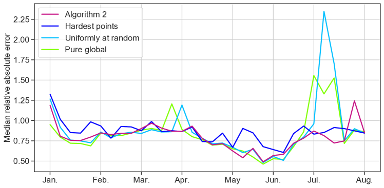
Figure 1: The median relative absolute deviation over all locations $\ell=1,\ldots,L$, at each time point $t=1,\ldots,T$, as in (27), when we use stacking and the subpopulation size $r\leq L/4$.

Table 1 shows the results, when the subpopulation size $r\leq L/4$. As we mentioned at the beginning of this section, we expect our methodology to not degrade overall performance too badly, i.e., to essentially perform on par with the global model. Interestingly, our method actually outperforms the other methods, including the global model, for three out of the four retraining strategies. The differences are most pronounced when using the two aggregated local strategies we described above (averaging and stacking), whereas performance is comparable when using either the shared strength or pure local strategy. As an alternative viewpoint, Figure 1 shows the median relative error at each time step, as in (27), when we use stacking. We can see that our methodology has more stable performance over time.

Tables 2 and 3 again show the global error, for $r\leq L/5$ and $r\leq L/6$, respectively. Of course, we do not expect our methodology to outperform the global model uniformly, for all values of the maximum region size. Indeed, we can see from the two tables that our methodology either performs best, or comparable to the best in a few cases. In particular, our methodology seems to work well when we use stacking or simple averaging, and is roughly on par with the other approaches when we use either the shared strength or pure local strategies. It is worth keeping in mind that in these latter cases, the (small) differences in performance come with the benefit of interpretability, as we discuss later. Still, the good performance of our method is slightly surprising (and encouraging), as we did not perform any tuning, e.g., of the metric or maximum size used to construct the regions that our method uses.

Local performance. Now we turn to briefly investigating local performance. In the absence of any “ground truth” subpopulations of interest (recall this was the reason we required the first pass that we described before), we simply compare the distributions of errors (27), for Algorithm 2 vs. those of the pure global benchmark, across the hardest subsets that Algorithm 2 identifies. Of course, we expect Algorithm 2 to exhibit better local performance than the global model in this case. We show a Q-Q plot in Figure 2, where we compare the quantiles of the distributions of errors (over all locations $\ell=1,\ldots,L$, and time points $t=1,\ldots,T$), for Algorithm 2 vs. the global model. We use stacking and set the subpopulation size $r\leq L/4$, for Algorithm 2. From the figure, we can indeed see that Algorithm 2 has better local performance.

Interpretability. Finally, we inspect and interpret a few of the regions themselves, again when $r\leq L/4$. We show the regions that Algorithm 2 produces on the 22nd of January 2021, 29th of January 2021, 16th of April 2021, and 30th of August 2021, in Figures 3, 4, 5, and 6, respectively. We also consider the regions that a “naive” baseline generates on the same days, i.e., the baseline that forms regions simply based on the counties with the highest scores. We show these latter regions in Figures 7, 8, 9, and 10, respectively. It is interesting to interpret the regions. On the 22nd and 29th of January 2021—widely recognized as two weeks with the highest incidence of COVID-19 in the United States at the time—our methodology (as in Figures 3 and 4) identifies two regions that seem to reflect the movement of the virus across the country (cf. Figures 11 and 12). Of course, as we expect, the regions from Algorithm 2 are in fact structured, meaning that they do not exclusively contain only the “hardest” counties, which can help with interpretability. On the other hand, the corresponding naive regions simply contain the hardest counties with no real structure present whatsoever.

On the 16th of April 2021—after several weeks of implementing precautionary measures—the state of Michigan saw a sudden spike in the incidence of COVID-19, which our methodology evidently completely captures; see Figure 5. On the other hand, the corresponding naive region (see Figure 13) does not include the entire state of Michigan, but rather just a few of the Michigan counties with the highest incidence of COVID-19, along with counties from other states.

Finally, on the 30th of August 2021, outbreaks began to emerge throughout the country, due to the rise of the Delta variant—with Arkansas and Missouri being two of the worst states. Again, our methodology, which we show in Figure 5, completely captures these two states.

	Retraining strategy
Subpopulation identification strategy	Averaging	Stacking	Multi-task	Pure local
Algorithm 2	0.7862	0.7885	0.8032	0.7859
Algorithm 2, unpenalized	0.7892	0.8026	0.8025	0.7968
Hardest points	0.8231	0.8813	0.8070	0.8022
Uniformly at random	0.8240	0.8170	0.8110	0.8180
Pure global	0.7909	0.7909	0.7909	0.7909

Table 1: The median relative absolute deviation over all locations $\ell=1,\ldots,L$, and time points $t=1,\ldots,T$, when the subpopulation size $r\leq L/4$. We highlight the best (i.e., lowest) error, for each retraining strategy, in bold.

	Retraining strategy
Subpopulation identification strategy	Averaging	Stacking	Multi-task	Pure local
Algorithm 2	0.7955	0.7933	0.8044	0.8058
Algorithm 2, unpenalized	0.7951	0.7859	0.8097	0.8048
Hardest points	0.8289	0.8832	0.8068	0.8047
Uniformly at random	0.8279	0.8091	0.8096	0.8190
Pure global	0.7909	0.7909	0.7909	0.7909

Table 2: The median relative absolute deviation over all locations $\ell=1,\ldots,L$, and time points $t=1,\ldots,T$, when the subpopulation size $r\leq L/5$. We highlight the best (i.e., lowest) error, for each retraining strategy, in bold.

	Retraining strategy
Subpopulation identification strategy	Averaging	Stacking	Multi-task	Pure local
Algorithm 2	0.8110	0.7907	0.8072	0.8336
Algorithm 2, unpenalized	0.8124	0.7923	0.8056	0.8315
Hardest points	0.8378	0.8525	0.8017	0.8340
Uniformly at random	0.8256	0.8092	0.8126	0.8187
Pure global	0.7909	0.7909	0.7909	0.7909

Table 3: The median relative absolute deviation over all locations $\ell=1,\ldots,L$, and time points $t=1,\ldots,T$, when the subpopulation size $r\leq L/6$. We highlight the best (i.e., lowest) error, for each retraining strategy, in bold.

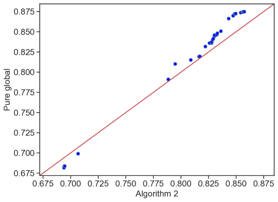
Figure 2: Q-Q plot comparing the distribution of Algorithm 2’s median relative absolute deviation (over all locations $\ell=1,\ldots,L$, and time points $t=1,\ldots,T$) on the hardest regions it identifies, vs. those of the pure global model on the same regions. We use stacking and set the subpopulation size $r\leq L/4$, for Algorithm 2.

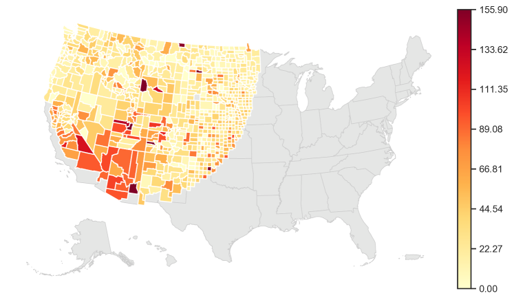
Figure 3: The hardest region that Algorithm 2 produces on the 22nd of January 2021, when we require the region size $r\leq L/4$. We color the counties according to the true number of COVID-19 cases per 100,000 people, smoothed over the previous week.

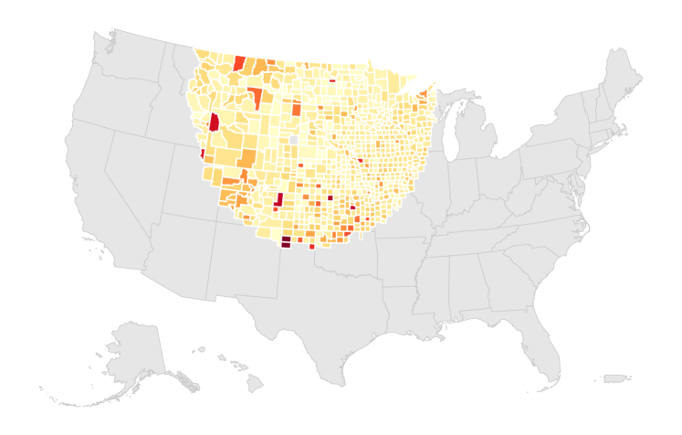
Figure 4: The hardest region that Algorithm 2 produces on the 29th of January 2021, when we require the region size $r\leq L/4$. We color the counties according to the true number of COVID-19 cases per 100,000 people, smoothed over the previous week.

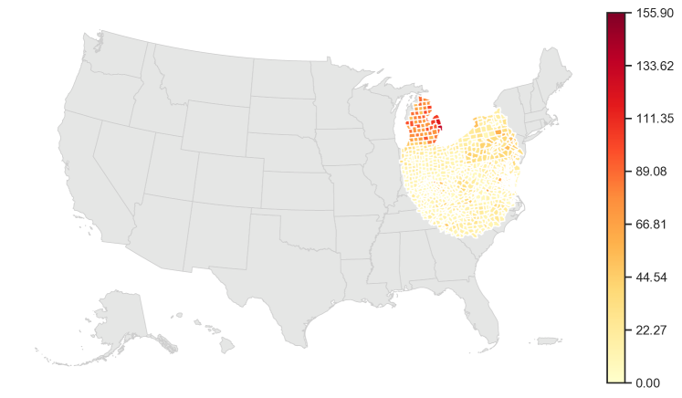
Figure 5: The hardest region that Algorithm 2 produces on the 16th of April 2021, when we require the region size $r\leq L/4$. We color the counties according to the true number of COVID-19 cases per 100,000 people, smoothed over the previous week.

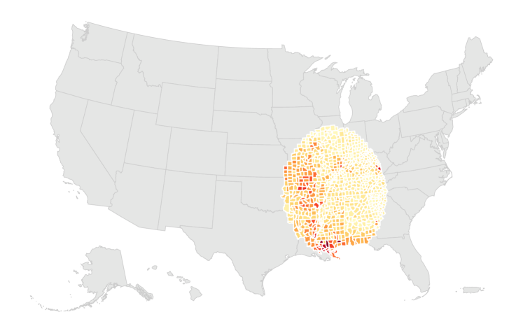
Figure 6: The hardest region that Algorithm 2 produces on the 30th of August 2021, when we require the region size $r\leq L/4$. We color the counties according to the true number of COVID-19 cases per 100,000 people, smoothed over the previous week.

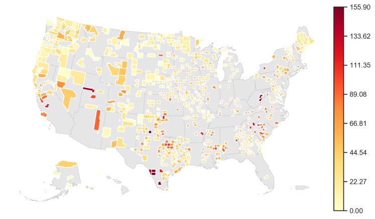
Figure 7: The hardest region the naive baseline produces on the 22nd of January 2021, when we require the region size $r\leq L/4$. We color the counties according to the true number of COVID-19 cases per 100,000 people, smoothed over the previous week.

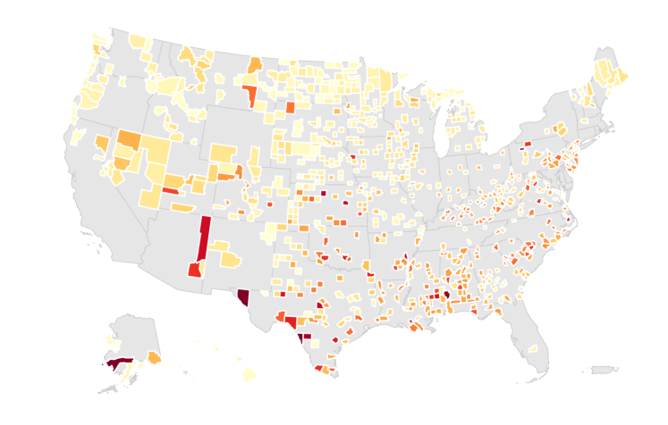
Figure 8: The hardest region the naive baseline produces on the 29th of January 2021, when we require the region size $r\leq L/4$. We color the counties according to the true number of COVID-19 cases per 100,000 people, smoothed over the previous week.

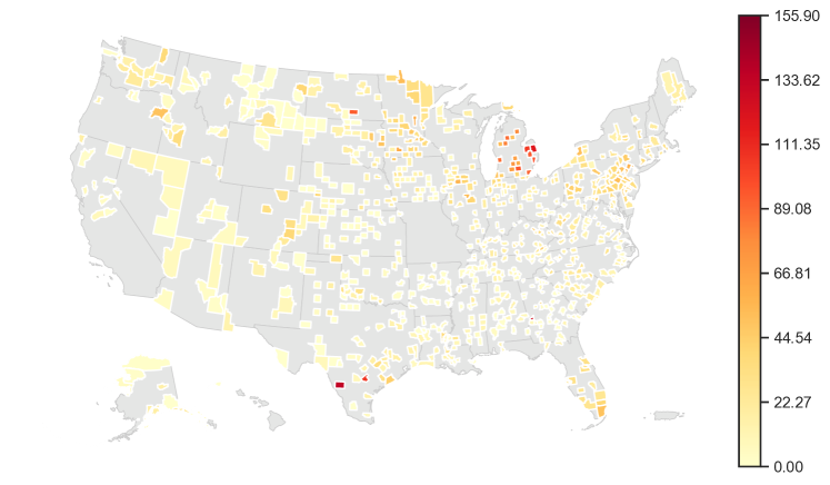
Figure 9: The hardest region the naive baseline produces on the 16th of April 2021, when we require the region size $r\leq L/4$. We color the counties according to the true number of COVID-19 cases per 100,000 people, smoothed over the previous week.

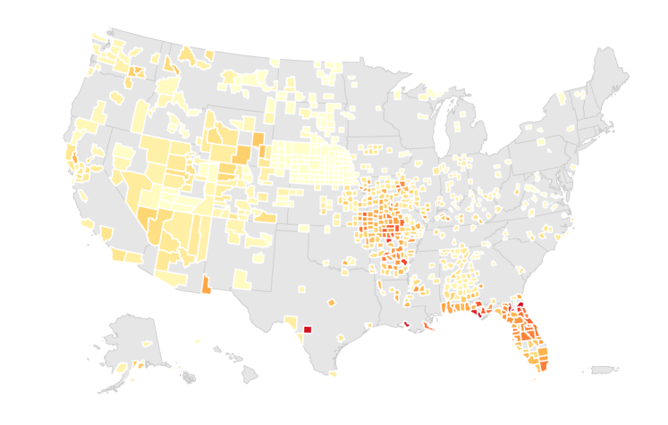
Figure 10: The hardest region the naive baseline produces on the 30th of August 2021, when we require the region size $r\leq L/4$. We color the counties according to the true number of COVID-19 cases per 100,000 people, smoothed over the previous week.

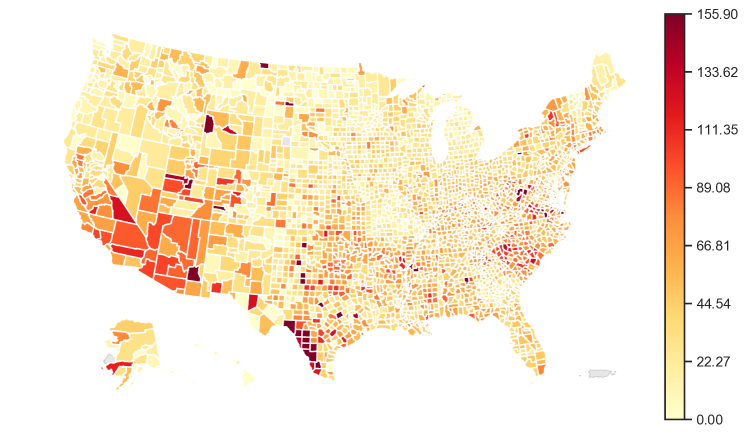
Figure 11: United States counties, which we color according to the true number of COVID-19 cases per 100,000 people, smoothed over the week of January 22, 2021.

Figure 12: United States counties, which we color according to the true number of COVID-19 cases per 100,000 people, smoothed over the week of January 29, 2021.

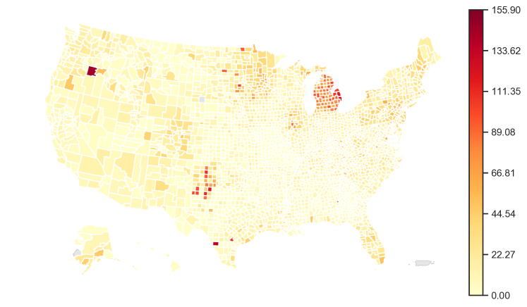
Figure 13: United States counties, which we color according to the true number of COVID-19 cases per 100,000 people, smoothed over the week of April 16, 2021.

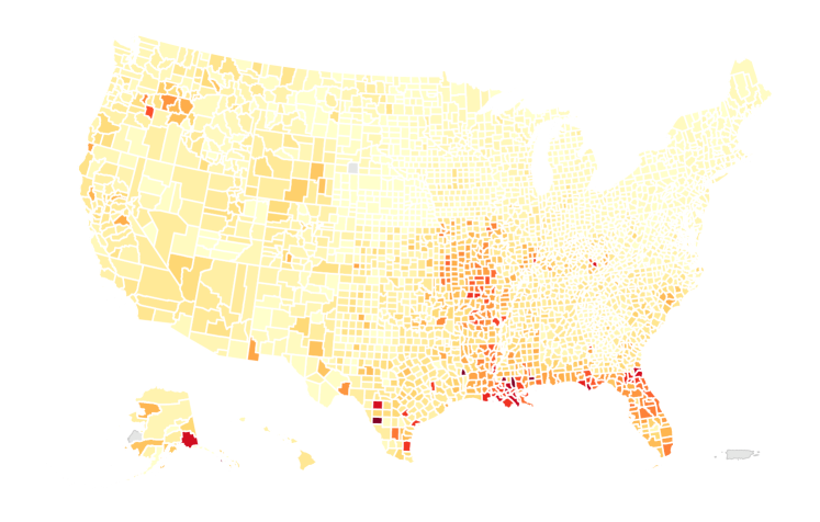
Figure 14: United States counties, which we color according to the true number of COVID-19 cases per 100,000 people, smoothed over the week of August 30, 2021.

6.2 Distribution shift adaptation

We now turn to a different experimental set-up, and test our methods on datasets with built-in distribution shifts. The WILDS project [42] gathers supervised learning datasets in which each instance has a “group” or domain attribute (sometimes several), such as the country or location the instance comes from, the identity of the reviewer that gave a certain rating, or the hospital/specific machine that produced the medical image to study. The existence of such attributes allows us to consider training, validation and test data as mixtures of sub-populations, that is distributions $\{P_{g}\}_{g\in\mathcal{G}}$, where $\mathcal{G}$ is the set of all different groups—countries, reviewers,hospitals—that form the entire dataset.

For both WILDS datasets that we investigate—poverty mapping [42] and Amazon reviews [42]—we follow the same general experimental procedure, which replicates a scenario where practitioners, aiming to improve their model and with limited additional (labeled) data available, need to decide how to best allocate their resources and where to gather new data instances.

1. We first train a model on a training set containing only a fraction of the entire groups, i.e. we train our model on $P_{0}^{\text{train}}=\sum_{g\in\mathcal{G}_{0}}\alpha^{\text{train}}_{g}P_{g}$ for a certain choice of mixture coefficients $\alpha^{\text{train}}_{g}>0$ and $\mathcal{G}_{0}\subsetneq\mathcal{G}$, and we compute non-conformity scores on an independent calibration set coming from the same restricted distribution $P_{0}^{\text{calib}}=P_{0}^{\text{train}}$.

2. On a first test set, which is now a mixture of all different sub-groups present in the dataset, i.e. $P_{0}^{\text{test}}=\sum_{g\in\mathcal{G}}\alpha^{\text{test}}_{g}P_{g}$ with $\alpha^{\text{test}}_{g}>0$ for all $g\in\mathcal{G}$, we identify a hard region $R\in\mathcal{R}$ using Algorithm 2, using as p-values the ranks of each test non-conformity score among all calibration scores.

3. We then refit a model by augmenting the training set with additional independent data from $P_{0}^{\text{test}}\mid X\in R^{\text{hard}}$, and compare it to two different baselines: one where the training set receives additional independent data from $P_{0}^{\text{test}}$ (“random”) and one where the training set receives data points that are neighbors of test instances with the highest ranks (“hardest”).

4. We eventually test the performance of each refitted model on a second independent test set (from $P_{0}^{\text{test}}$).

Remark     In our experiments, we choose every coefficient $\alpha_{g}^{\text{train}},\alpha_{g}^{\text{test}}$ proportionally to the amount of instances from the sub-population in the entire dataset available.

The goal of our experimental procedure is two-fold. First, since our initial model did not have access to any sample from $\{P_{g}\}_{g\notin\mathcal{G}_{0}}$, we expect it to perform poorly on these, and hence to detect a region $R^{\text{hard}}$ comprising mostly of examples from these unseen groups, which would correspond to having

$$P_{0}^{\text{test}}\mid X\in R^{\text{hard}}\simeq\sum_{g\in\mathcal{G}\setminus\mathcal{G}_{0}}\alpha_{g}^{\text{hard}}P_{g}.$$ (28)

In particular, we expect our procedure to be less sensitive to noise and outliers than the more naive “Hardest” method, which simply includes samples with very high scores and does not take any feature structure into account.

If our first hypothesis (28) holds (at least partially), we then would expect, during the second training phase, a larger improvement in performance on these sub-groups with our method than with the two other baseline procedures, which add the same amount of data to the training set, but in a less targeted fashion. We thus hope that our method shows better or equivalent average performance on $P_{0}^{\text{test}}$, but even more so that it significantly outperforms both baselines on each sub-population $\{P_{g}\}_{g\in\mathcal{G}\setminus\mathcal{G}_{0}}$.

Crucially, in these experiments, we only use knowledge of the group or protected attribute $g\in\mathcal{G}$ to construct the distributions $P_{0}^{\text{train}}$ and $P_{0}^{\text{test}}$: none of the methods has access to that piece of information to choose which instances to train with. Even if we expect the model to display group-heterogeneous performance, our method (Alg. 2) cannot use it directly as a discriminant: the hypothesis is that examples from the same group should also cluster, at least partially, in the feature space.

6.2.1 Poverty mapping

We first experiment with the poverty map dataset [42], where we aim to predict the poverty level across spatial regions from satellite imagery, precisely their asset wealth index. A notable challenge of this problem is the scarcity of poverty level measurements in some regions of the world, especially in comparison with the wide availability of unlabeled satellite imagery: this calls for models robust and adaptive to geographical distribution shifts, and allows us to test our methodology. The group or sub-population $g\in\mathcal{G}$ of each instance is the country where the image comes from; the data originates from $|\mathcal{G}|=23$ different countries, among which four of them ($\mathcal{G}\setminus\mathcal{G}_{0}=\{\text{Cameroon, Ghana, Malawi, Zimbabwe}\}$) only appear in the test distribution $P_{0}^{\text{test}}$.

We train all our models using the default network architecture and hyper-parameters in the WILDS package, minimizing the average least-squares loss—this corresponds to the ERM algorithm with a ResNet18-MS model. By doing so, we make sure that the distribution of each respective training set is the only difference between our different models that we compare.

In our experiments, when applying Alg. 2 we vary one additional parameter $\delta\in(0,1)$, which controls the maximum size of the hard region that Alg. 2 can detect. The reason why we need such parameter is simple: in real datasets, it is plausible that large sub-populations of the data (and not simply are actually much harder to predict or classify that some others, hence with ranks significantly higher than uniform: this could (and in some cases, would) lead Alg 2 to focus on regions that are potentially too large to be of practical use. This is why we focus on detecting regions $R^{\text{hard}}$ such that $P_{0}^{\text{test}}(X\in R^{\text{hard}})\leq\delta$: our goal is to detect reasonably small regions, with the hope that they overlap with hard out of domain instances. Finally, the set of regions on which we apply our detection method is the set of euclidean balls around the test points in the first test set, with the caveat that we use as feature vector $x\in\mathbb{R}^{d}$ the output of the pooling layer that precedes the last layer (and not the initial image itself), thus allowing the dimension of the problem to be lower.

We display our results in the three plots comprising Figure 15, and summarize them in Table 4. They are consistent with our initial expectations: Algorithm 2 offers a bigger performance improvement to the Baseline model than the more naive “Hardest point” and “Random” methods, across the whole range of different $\delta$, whether in terms of average error or out of domain error, the latter improvement being more significant. Additionally, the difference in performance between each method tends to increase as function of $\delta$, meaning that for this specific dataset and sub-populations choices, it appears beneficial to allow for a large hard region, potentially because the performance of the model is particularly heterogeneous across different regions of the world.

		Type of mean squared error
$\delta$	Subpopulation identification strategy	Average	O.O.D Region	Hard Region
0.10	Algorithm 2	0.2157(0.0195)	0.3028(0.0179)	0.3872(0.0267)
	Hardest points	0.2257(0.0128)	0.3229(0.0114)	0.4101(0.0289)
	Uniformly at random	0.2273(0.0133)	0.3228(0.0128)	0.4112(0.0289)
	Baseline	0.2586(0.0111)	0.3333(0.0252)	0.4847(0.0574)
0.15	Algorithm 2	0.2151(0.0161)	0.3037(0.0155)	0.3651(0.0262)
	Hardest points	0.2288(0.0141)	0.3276(0.0144)	0.3904(0.0305)
	Uniformly at random	0.2298(0.0157)	0.3244(0.0126)	0.3891(0.0321)
	Baseline	0.2586(0.0111)	0.3333(0.0252)	0.4633(0.0528)
0.20	Algorithm 2	0.2215(0.022)	0.3077(0.0184)	0.3544(0.0315)
	Hardest points	0.2258(0.0114)	0.3234(0.0091)	0.3694(0.0275)
	Uniformly at random	0.2376(0.0337)	0.3301(0.0276)	0.3744(0.0374)
	Baseline	0.2586(0.0111)	0.3333(0.0252)	0.4467(0.0388)
0.25	Algorithm 2	0.2166(0.0245)	0.2988(0.0204)	0.341(0.0345)
	Hardest points	0.2284(0.0156)	0.3265(0.0132)	0.3606(0.0264)
	Uniformly at random	0.2277(0.0124)	0.3206(0.0101)	0.3581(0.0239)
	Baseline	0.2586(0.0111)	0.3333(0.0252)	0.4292(0.038)
0.30	Algorithm 2	0.2092(0.016)	0.2928(0.0169)	0.3157(0.0175)
	Hardest points	0.2300(0.0108)	0.3261(0.0081)	0.3435(0.0151)
	Uniformly at random	0.2269(0.0109)	0.3231(0.009)	0.3418(0.0157)
	Baseline	0.2586(0.0111)	0.3333(0.0252)	0.4032(0.0157)

Table 4: Mean squared error, averaged over $M=10$ trials, for different values of $\delta\in\{0.1,0.15,0.2,0.25,0.3\}$, in the poverty map dataset. We report three types of error: the average error over an independent test set from $P_{0}^{\text{test}}$ (data from every $\{P_{g}\}_{g\in\mathcal{G}}$), the average error over the test set restricted to out of domain data (data only from $\{P_{g}\}_{g\notin\mathcal{G}_{0}}$), and the average error over the hard region $P_{0}^{\text{test}}\mid X\in R^{\text{hard}}$ that Algorithm 2 detects—we of course expect our method to show better performance on the latter, so we report it more as a sanity check. We highlight the best (i.e., lowest) error, for each type of error strategy, in bold, and report the standard deviation over $M=10$ trials in parentheses.

\begin{overpic}[scale={0.5}]{figs/poverty_map_avg.pdf} \put(0.0,10.0){ \leavevmode\hbox to6.09pt{\vbox to171.12pt{\text{[drawing]}}} } \put(0.0,10.0){\rotatebox{90.0}{ \small Average mean squared error} } \put(40.0,0.0){ \leavevmode\hbox to114.21pt{\vbox to10.36pt{\text{[drawing]}}} } \put(50.0,1.0){ \small$\delta$} \par\par\end{overpic}

\begin{overpic}[scale={0.5}]{figs/poverty_map_ood_region.pdf} \put(0.0,10.0){ \leavevmode\hbox to6.09pt{\vbox to171.12pt{\text{[drawing]}}} } \put(0.0,10.0){\rotatebox{90.0}{ \small O.O.D mean squared error} } \put(40.0,0.0){ \leavevmode\hbox to114.21pt{\vbox to10.36pt{\text{[drawing]}}} } \put(50.0,1.0){ \small$\delta$} \par\par\end{overpic}

\begin{overpic}[scale={0.5}]{figs/poverty_map_hard_region.pdf} \put(0.0,10.0){ \leavevmode\hbox to6.09pt{\vbox to171.12pt{\text{[drawing]}}} } \put(0.0,10.0){\rotatebox{90.0}{ \small Hard region mean squared error} } \put(40.0,0.0){ \leavevmode\hbox to114.21pt{\vbox to10.36pt{\text{[drawing]}}} } \put(50.0,1.0){ \small$\delta$} \par\par\end{overpic}

Figure 15: Mean squared error, averaged over $M=10$ trials, for different values of $\delta\in\{0.1,0.15,0.2,0.25,0.3\}$, in the poverty map dataset. We report three types of error (one for each plot): the average error over an independent test set from $P_{0}^{\text{test}}$ (data from every $\{P_{g}\}_{g\in\mathcal{G}}$), the average error over the test set restricted to out of domain data (data only from $\{P_{g}\}_{g\notin\mathcal{G}_{0}}$), and the average error over the hard region $P_{0}^{\text{test}}\mid X\in R^{\text{hard}}$ that Alg. 2 detects—we of course expect our method to show better performance on the latter, so we only report it more as a sanity check. The “Baseline” method is the initial model, consisting of data from $P_{0}^{\text{train}}$. We report error bars as twice the standard error over the $M$ trials.

6.2.2 Review rating prediction

We next study the impact of weak supervision on our methods, experimenting on the Amazon review dataset [42]. The goal here is to predict what rating on a scale from 1 to 5 some user left based on the comment they wrote; each particular user represents a different sub-population, and the out-of-domain region simply is a set of users for which none of their comments belongs to the training set.

The Amazon review dataset is fully supervised, meaning that all ratings $Y\in[5]$ are available. However, for the purpose of testing our method in a partially labeled setting, we introduce weak supervision in the first test set, i.e. when finding hard regions with Alg. 2. Specifically, instead of observing the actual rating $Y$, we assume that we only have access to a “noisy” version of it, namely an interval $Y_{\text{weak}}\coloneqq[Y_{\text{min}},Y_{\text{max}}]\subset[1,5]$ that contains the true rating $Y$. For instance, if the initial true rating was $Y=4$, we could only observe $Y_{\text{weak}}=\{3,4,5\}$. For simplicity, we introduce partial supervision in the following way: for each instance, $x,y\in\mathcal{X}\times[5]$, and for some real parameter $c>0$, we have

$$p(y_{\text{weak}}=[y_{\text{min}},y_{\text{max}}]\mid x,y)\propto e^{-c\left(y_{\text{max}}-y_{\text{min}}\right)}1\!\left\{y\in y_{\text{weak}}\right\},$$

which means that the distribution of the partial label only depends on the actual rating (probably too simplistic in practice), and that the probability of the size of the interval decreases exponentially. The parameter $c>0$ controls the average size of the “weak” label set: the bigger it is, the closer to full supervision we are. We run our forthcoming experiments with values of $c>0$ such that $\mathbb{E}\left[\left|Y_{\text{weak}}\right|\right]\in\{1.2,1.5\}$, to compare two different noise levels of weak supervision. We plot the distribution of the weak label size $|Y_{\text{weak}}|$ conditionally on the label $Y$ in Figure 16.

Similarly to the poverty map experiment, we report the average accuracy of the different methods on three different groups: the entire distribution, the out of domain region, and the hard region Alg. 2 unveils. Additionally, to evaluate out-of-domain performance, for each method and out-of-domain user, we compute the average accuracy and compare it to its baseline counterpart. This results, for each method, in a distribution of the difference in accuracy over the set of O.O.D. users; we then report the c.d.f. of that distribution as a measure of improvement over out-of-domain reviews (see Figure 17).

To provide a comparison baseline, we run the same methods as in the previous Section in the full supervision setting, and report our results in Figure 17A and Table 5. Our findings here are consistent with the conclusions we previously drew, in the sense that Alg. 2 allows a small but significant improvement of performance over the more naive methods “Hardest” and “Random” methods.

The comparison for the partially labeled setting has more nuances. To run Alg. 2, we now use as test and calibration scores the min-scores as in Eqn. (2). In most instances, especially in high accuracy tasks, they are equal to the true scores,which is why we would expect our results in the partially supervised setting to echo those in the fully supervised regime. This is only partially the case: when introducing small label noise (i.e., $\mathbb{E}\left[\left|Y_{\text{weak}}\right|\right]=1.2$), our method indeed generates models with higher accuracies in and out of domain, as we outline in Table 6 and 7, and Figures 17B/C. On the other hand, when weak supervision is inherently noisier (i.e, $\mathbb{E}|Y_{\text{weak}}|=1.5$ is larger), Table 7 shows that the “Hardest” method is on-par or even better than Alg. 2 for larger sizes $\delta>0$: it is possible that weak supervision combined with larger sizes of hard subsets have itself an implicit regularization effect on that more naive method, resulting in better performance.

\begin{overpic}[scale={0.5}]{figs/amazon_review_partial_ws_size_12.pdf} \put(2.0,10.0){ \leavevmode\hbox to6.09pt{\vbox to171.12pt{\text{[drawing]}}} } \put(2.0,20.0){\rotatebox{90.0}{ \small$\mathbb{P}(|Y_{\text{weak}}|\leq t\mid Y=y)$} } \put(40.0,2.0){ \leavevmode\hbox to114.21pt{\vbox to10.36pt{\text{[drawing]}}} } \put(47.0,3.0){ \small$t$} \end{overpic}

\begin{overpic}[scale={0.5}]{figs/amazon_review_partial_ws_size_15.pdf} \put(2.0,10.0){ \leavevmode\hbox to6.09pt{\vbox to171.12pt{\text{[drawing]}}} } \put(2.0,20.0){\rotatebox{90.0}{ \small$\mathbb{P}(|Y_{\text{weak}}|\leq t\mid Y=y)$} } \put(40.0,2.0){ \leavevmode\hbox to114.21pt{\vbox to10.36pt{\text{[drawing]}}} } \put(47.0,2.0){ \small$t$} \par\end{overpic}

Figure 16: Distribution of the weak label set size $|Y_{\text{weak}}|$ in the Amazon review dataset experiment, for two different values of the parameter $c>0$ corresponding to respective average sizes $\mathbb{E}|Y_{\text{weak}}$ of $1.2$ (left plot) and $1.5$ (right plot).

		Type of average accuracy
$\delta$	Subpopulation identification strategy	Average	O.O.D Region	Hard Region
0.05	Algorithm 2	0.7312(0.0015)	0.7232(0.0017)	0.4584(0.0066)
	Baseline	0.7292(0.0018)	0.7204(0.003)	0.4386(0.0057)
	Hardest points	0.7297(0.0013)	0.7205(0.0022)	0.4458(0.0041)
	Uniformly at random	0.73(0.002)	0.7211(0.0026)	0.4463(0.0077)
0.10	Algorithm 2	0.7327(0.0014)	0.726(0.0024)	0.5122(0.0049)
	Baseline	0.7292(0.0018)	0.7204(0.003)	0.4919(0.0048)
	Hardest points	0.7312(0.0022)	0.7234(0.003)	0.5027(0.004)
	Uniformly at random	0.7311(0.0014)	0.723(0.0022)	0.5008(0.0034)
0.15	Algorithm 2	0.7335(0.0013)	0.7267(0.0016)	0.5433(0.0031)
	Baseline	0.7292(0.0018)	0.7204(0.003)	0.525(0.0054)
	Hardest points	0.7327(0.002)	0.7254(0.0038)	0.5374(0.0035)
	Uniformly at random	0.7313(0.0018)	0.7232(0.003)	0.5329(0.0038)

Table 5: Accuracy for different values of $\delta\in\{0.05,0.10,0.15\}$, in the Amazon review dataset in the fully supervised regime. We report three types of accuracy: the average accuracy over an independent test set from $P_{0}^{\text{test}}$ (data from every $\{P_{g}\}_{g\in\mathcal{G}}$), the average accuracy over the test set restricted to out of domain data (data only from $\{P_{g}\}_{g\notin\mathcal{G}_{0}}$), and the average accuracy over the hard region $P_{0}^{\text{test}}\mid X\in R^{\text{hard}}$ that Algorithm 2 detects. We highlight the best accuracy for each type of population and report the standard deviation over $M=5$ trials in parentheses.

		Type of average accuracy
$\delta$	Subpopulation identification strategy	Average	O.O.D Region	Hard Region
0.05	Algorithm 2	0.732(0.0012)	0.7251(0.0021)	0.4648(0.0065)
	Baseline	0.7288(0.0021)	0.721(0.0037)	0.4338(0.0053)
	Hardest points	0.7303(0.0018)	0.7226(0.003)	0.4526(0.0059)
	Uniformly at random	0.7304(0.0018)	0.723(0.0036)	0.4472(0.007)
0.10	Algorithm 2	0.7326(0.002)	0.7268(0.0037)	0.5141(0.0081)
	Baseline	0.7288(0.0021)	0.721(0.0037)	0.4925(0.0047)
	Hardest points	0.7309(0.0023)	0.7239(0.0029)	0.5029(0.0066)
	Uniformly at random	0.7311(0.0019)	0.725(0.003)	0.504(0.0073)
0.15	Algorithm 2	0.7327(0.0015)	0.7272(0.0034)	0.558(0.0162)
	Baseline	0.7288(0.0021)	0.721(0.0037)	0.5411(0.0206)
	Hardest points	0.7325(0.0023)	0.7264(0.0027)	0.5524(0.0177)
	Uniformly at random	0.7315(0.0017)	0.7255(0.0032)	0.5503(0.0183)

Table 6: Accuracy for different values of $\delta\in\{0.05,0.10,0.15\}$, in the Amazon review dataset in the partially supervised regime, with an average size $\mathbb{E}\left[|Y_{\text{weak}}|\right]=1.2$.

		Type of average accuracy
$\delta$	Subpopulation identification strategy	Average	O.O.D Region	Hard Region
0.05	Algorithm 2	0.731(0.0009)	0.7235(0.0031)	0.4653(0.0127)
	Baseline	0.7283(0.0012)	0.7199(0.002)	0.4431(0.0112)
	Hardest points	0.7296(0.0011)	0.7223(0.0038)	0.4538(0.0104)
	Uniformly at random	0.7296(0.0017)	0.7219(0.0032)	0.4498(0.0183)
0.10	Algorithm 2	0.7306(0.001)	0.7243(0.0018)	0.5493(0.0304)
	Baseline	0.729(0.0015)	0.7214(0.0034)	0.5308(0.0314)
	Hardest points	0.7314(0.001)	0.7237(0.0029)	0.5447(0.0333)
	Uniformly at random	0.7304(0.0012)	0.7236(0.0037)	0.5401(0.0332)
0.15	Algorithm 2	0.7314(0.0009)	0.7244(0.0024)	0.5758(0.0149)
	Baseline	0.7264(0.0049)	0.7186(0.0046)	0.5577(0.0213)
	Hardest points	0.7323(0.0015)	0.7251(0.003)	0.5722(0.018)
	Uniformly at random	0.7314(0.0013)	0.7244(0.0028)	0.5685(0.0166)

Table 7: Accuracy for different values of $\delta\in\{0.05,0.10,0.15\}$, in the Amazon review dataset in the partially supervised regime, with an average size $\mathbb{E}\left[|Y_{\text{weak}}|\right]=1.5$.

\begin{overpic}[scale={0.5}]{figs/amazon_review_full_cdf_per_user.pdf} \par\put(0.0,4.0){ \leavevmode\hbox to8.94pt{\vbox to114.21pt{\text{[drawing]}}} } \put(0.0,3.0){\rotatebox{90.0}{ \small$\mathbb{P}_{\text{user}}\left[\Delta_{\text{Acc,User,Method}}\leq t\right]$} } \put(11.0,1.0){ \leavevmode\hbox to114.21pt{\vbox to10.36pt{\text{[drawing]}}} } \put(38.0,1.0){ \leavevmode\hbox to114.21pt{\vbox to10.36pt{\text{[drawing]}}} } \put(65.0,1.0){ \leavevmode\hbox to114.21pt{\vbox to10.36pt{\text{[drawing]}}} } \par\put(17.0,1.0){ \small$t$ } \put(46.0,1.0){ \small$t$ } \put(73.0,1.0){ \small$t$ } \par\par\put(13.0,27.5){ \leavevmode\hbox to114.21pt{\vbox to8.94pt{\text{[drawing]}}} } \put(42.0,27.5){ \leavevmode\hbox to114.21pt{\vbox to8.94pt{\text{[drawing]}}} } \put(69.0,27.5){ \leavevmode\hbox to114.21pt{\vbox to8.94pt{\text{[drawing]}}} } \par\put(15.0,28.0){ \small$\delta=0.05$ } \put(42.0,28.0){ \small$\delta=0.10$ } \put(69.0,28.0){ \small$\delta=0.15$ } \put(90.0,28.0){{A}} \end{overpic}

\begin{overpic}[scale={0.5}]{figs/amazon_review_partial_12_cdf_per_user.pdf} \par\put(0.0,4.0){ \leavevmode\hbox to8.94pt{\vbox to114.21pt{\text{[drawing]}}} } \put(0.0,3.0){\rotatebox{90.0}{ \small$\mathbb{P}_{\text{user}}\left[\Delta_{\text{Acc,User,Method}}\leq t\right]$} } \put(11.0,1.0){ \leavevmode\hbox to85.76pt{\vbox to10.36pt{\text{[drawing]}}} } \put(38.0,1.0){ \leavevmode\hbox to114.21pt{\vbox to10.36pt{\text{[drawing]}}} } \put(65.0,1.0){ \leavevmode\hbox to114.21pt{\vbox to10.36pt{\text{[drawing]}}} } \par\put(17.0,1.0){ \small$t$ } \put(46.0,1.0){ \small$t$ } \put(73.0,1.0){ \small$t$ } \par\par\put(13.0,27.5){ \leavevmode\hbox to114.21pt{\vbox to8.94pt{\text{[drawing]}}} } \put(42.0,27.5){ \leavevmode\hbox to114.21pt{\vbox to8.94pt{\text{[drawing]}}} } \put(69.0,27.5){ \leavevmode\hbox to114.21pt{\vbox to8.94pt{\text{[drawing]}}} } \par\put(15.0,28.0){ \small$\delta=0.05$ } \put(46.0,28.0){ \small$\delta=0.10$ } \put(69.0,28.0){ \small$\delta=0.15$ } \put(90.0,28.0){{B}} \end{overpic}

\begin{overpic}[scale={0.5}]{figs/amazon_review_partial_15_cdf_per_user.pdf} \put(0.0,4.0){ \leavevmode\hbox to8.94pt{\vbox to114.21pt{\text{[drawing]}}} } \put(0.0,3.0){\rotatebox{90.0}{ \small$\mathbb{P}_{\text{user}}\left[\Delta_{\text{Acc,User,Method}}\leq t\right]$} } \put(11.0,1.0){ \leavevmode\hbox to114.21pt{\vbox to10.36pt{\text{[drawing]}}} } \put(38.0,1.0){ \leavevmode\hbox to114.21pt{\vbox to10.36pt{\text{[drawing]}}} } \put(65.0,1.0){ \leavevmode\hbox to114.21pt{\vbox to10.36pt{\text{[drawing]}}} } \par\put(17.0,1.0){ \small$t$ } \put(42.0,1.0){ \small$t$ } \put(73.0,1.0){ \small$t$ } \par\par\put(13.0,27.5){ \leavevmode\hbox to114.21pt{\vbox to8.94pt{\text{[drawing]}}} } \put(42.0,27.5){ \leavevmode\hbox to114.21pt{\vbox to8.94pt{\text{[drawing]}}} } \put(69.0,27.5){ \leavevmode\hbox to114.21pt{\vbox to8.94pt{\text{[drawing]}}} } \par\put(15.0,28.0){ \small$\delta=0.05$ } \put(42.0,28.0){ \small$\delta=0.10$ } \put(69.0,28.0){ \small$\delta=0.15$ } \put(90.0,28.0){{C}} \end{overpic}

Figure 17: Results for the Amazon review dataset, with panel A being the fully supervised setting $\mathbb{E}\left[|Y_{\text{weak}}|\right]=1$, panel B having a small amount of weak supervision $\mathbb{E}\left[|Y_{\text{weak}}|\right]=1.2$ and panel C having the noisiest labels $\mathbb{E}\left[|Y_{\text{weak}}|\right]=1.5$. Define for each user and each method $\Delta_{\text{Acc,User,Method}}\coloneqq\text{Accuracy}_{\text{Method}}-\text{Accuracy}_{\text{Baseline}}$ to be the difference in accuracy between the method and the baseline. We report the cumulative distribution function of that quantity over the set of out-of-domain users, hence lower c.d.f.s are better (as it means the distribution is stochastically larger). The “Baseline” method has only seen data from $P_{0}^{\text{train}}$, so we expect all methods to improve upon it. We average each per-user accuracy over $M=5$ independent trials.

7 Discussion

We proposed inferential methodology for the localization and detection of subpopulations present in a data stream. Though we focused heavily on the implications for model maintenance, the underlying ideas apply more broadly, and reduce to familiar existing methodology in special cases. For example, when the class $\mathcal{R}$ is completely unstructured, i.e., $\mathcal{R}=2^{[n]}$, then Algorithm 1 essentially reduces to the Benjamini-Hochberg-type proposal of Bates et al. [9], for unstructured one-class outlier detection. On the other hand, when the class $\mathcal{R}$ is highly structured, e.g., satisfying certain geometric or graph-theoretic criteria, and we are additionally willing to make certain (parametric) assumptions about the data-generating process, then Algorithm 2 roughly becomes the familiar scan statistic (e.g., Kulldorff [44], Sharpnack et al. [58]).

There are other seemingly natural methodological approaches that we might have pursued. As we mentioned in Section 1, two-sample testing is intimiately connected to the ideas in the current paper, and the well-known Kolmogorov-Smirnov test [43, 60, 2] is probably one of the most widely used tools for nonparametric hypothesis testing. However, it is not immediately clear (at least to us) how we might modify the Kolmogorov-Smirnov test to work without making strong distributional assumptions about the underlying black box machine learning model, or for the purpose of localization. Additionally, it is reasonable to suggest that we use clustering for subgroup estimation, as part of the three-step approach to model refitting that we described in Section 5. However, it is also not clear what the type 1 and 2 error rates of such a procedure might be (and, moreover, how to control them). Nonetheless, exciting recent work has drawn connections between classification and two-sample testing [41], and therefore this may indeed be a fruitful direction to investigate.

Finally, a direction that seems interesting to pursue is developing a truly sequential version of the methodology we laid out here, i.e., to marry the ideas from the broad literature on sequential testing [8, 39, 40, 35, 36], with the ones in the current paper. More generally, we hope the methodology in this paper motivates others to consider the many challenges related to real-time monitoring and maintenance.

Appendix A Proofs

A.1 Proof of Theorem 1

We begin with a bit of notation. For $i\in[n]$, we have $Z_{i}=\mu 1\!\left\{i\in R^{\star}\right\}+\sigma\xi_{i}$ where $\xi_{i}\stackrel{{\scriptstyle\rm iid}}{{\sim}}\mathsf{N}(0,1)$. Recalling that $\mathcal{R}=\mathcal{R}_{\mathcal{X}}\cap\{X_{i}\}_{i=1}^{n}$, for each $R\in\mathcal{R}$ we define the localized noise

$$\xi(R)\coloneqq\frac{1}{\sigma\sqrt{|R|}}\sum_{i\in R}\xi_{i},$$

which are marginally standard normal, and the following correlation distance on sets in $\mathcal{R}$:

$$d_{\textup{cor}}(R_{1},R_{2})^{2}\coloneqq\frac{1}{2}\mathbb{E}[(\xi(R_{1})-\xi(R_{2}))^{2}]=1-\frac{|R_{1}\cap R_{2}|}{\sqrt{|R_{1}||R_{2}|}}.$$

The starting point of our proof is a type of basic inequality [cf. 69] relating the error in recovering $R^{\star}$ to penalized deviations of $\xi(R)$. Recall that $\widehat{R}$ maximizes $Z_{R}-\sigma\mathsf{reg}(R)$ for the penalty function $\mathsf{reg}(R)=C\sqrt{d\log\frac{en}{|R|\vee d}}$, so that by maximality of $\widehat{R}$, we have

$$\mu\frac{|\widehat{R}\cap R^{\star}|}{\sqrt{|\widehat{R}|}}+\sigma\xi(\widehat{R})-\sigma\mathsf{reg}(\widehat{R}) =Z_{\widehat{R}}-\sigma\mathsf{reg}(\widehat{R})$$

$$\geq Z_{R^{\star}}-\sigma\mathsf{reg}(R^{\star})=\mu\sqrt{|R^{\star}|}+\sigma\xi(R^{\star})-\sigma\mathsf{reg}(R^{\star})$$

Dividing by $\sqrt{|R^{\star}|}$ and rearranging, this is equivalent to the basic inequality

$$d_{\textup{cor}}^{2}(\widehat{R},R^{\star})\leq\frac{\sigma}{\mu\sqrt{|R^{\star}|}}\left(\mathsf{reg}(R^{\star})-\mathsf{reg}(\widehat{R})+\xi(\widehat{R})-\xi(R^{\star})\right).$$ (29)

We now proceed with a peeling argument by controlling the deviation on the right-hand-side of the basic inequality (29) over $d_{\textup{cor}}$-balls around $R^{\star}$. Our first step is to exhibit an equivalence between Hamming and correlation distances. (See Sec. A.1.1 for a proof.)

Lemma A.1.

Let $R_{1},R_{2}\in\mathcal{R}$. Then

$$d_{\textup{cor}}^{2}(R_{1},R_{2})\leq\frac{d_{\textup{ham}}(R_{1},R_{2})}{\max\{|R_{1}|,|R_{2}|\}}.$$

If additionally $d_{\textup{cor}}^{2}(R_{1},R_{2})\leq\frac{1}{2}$, then

$$\frac{d_{\textup{ham}}(R_{1},R_{2})}{3\min\{|R_{1}|,|R_{2}|\}}\leq d_{\textup{cor}}^{2}(R_{1},R_{2}).$$

To perform our peeling argument, for $\delta\in[0,1]$ we define the sets

$$\mathcal{R}_{\textup{cor}}(\delta)\coloneqq\left\{R\in\mathcal{R}\mid d_{\textup{cor}}(R,R^{\star})\leq\delta\right\},$$

and for all $\ell\in\{1,\dots,n\}$,

$$\mathcal{R}_{\ell}\coloneqq\left\{R\in\mathcal{R}\mid|R|\geq\ell\right\}.$$

Using an entropy integral bound [e.g. 69, Ch. 5.3], we can then claim the following lemma, whose proof we defer to Section A.1.2.

Lemma A.2.

There exists a numerical constant $C$ such that, for $r\in[0,1]$ and $\ell\in[n]$,

$$\mathbb{E}\left[\sup_{R\in\mathcal{R}_{\textup{cor}}(r)\cap\mathcal{R}_{\ell}}\left|\xi(R)-\xi(R^{\star})\right|\right]\leq C\left\{dr^{2}\log\frac{en}{(d\vee r^{2}\ell)}\right\}^{1/2}.$$

We combine the expectation bounds in Lemma A.2 with Gaussian Lipschitz concentration inequalities, along with the basic inequality (29), to obtain our final desired result. For any fixed $R_{1},R_{2}$, we have

$$\bigg{\|}{\frac{1}{\sqrt{|R_{1}|}}\mathbf{1}_{R_{1}}-\frac{1}{\sqrt{|R_{2}|}}\mathbf{1}_{R_{2}}}\bigg{\|}_{2}^{2}=2d_{\textup{cor}}^{2}(R_{1},R_{2}),$$

so that the function $f_{R}(z)\coloneqq\frac{1}{\sqrt{|R|}}\mathbf{1}_{R}^{T}z-\frac{1}{\sqrt{|R^{\star}|}}\mathbf{1}_{R^{\star}}^{T}z$ is $\sqrt{2}r^{2}$-Lipschitz for all $R\in\mathcal{R}_{\textup{cor}}(r)$. As a consequence, the concentration of Lipschitz functions of Gaussian vectors [e.g. 69, Thm. 2.26] yields that there exists a numerical constant $C$ such that for any $r\in[0,1]$, $\ell\in[n]$, and $t>0$, we have

$$\mathbb{P}\left(\sup_{R\in\mathcal{R}_{\textup{cor}}(r)\cap\mathcal{R}_{\ell}}\left|\xi(R)-\xi(R^{\star})\right|\geq C\sqrt{dr^{2}\log\frac{en}{d\vee(r^{2}\ell)}+r^{2}t}\right)\leq\exp(-t).$$ (30)

Lemma A.1 additionally implies $d_{\textup{ham}}(R,R^{\star})\leq 3kd_{\textup{cor}}^{2}(R,R^{\star})$ for all $R\in\mathcal{R}_{\textup{cor}}(1/\sqrt{2})$, where we recall $k=|R^{\star}|$. In particular, $|R|\geq|R^{\star}|(1-3r^{2})\geq\frac{k}{2}$, meaning $\mathcal{R}_{\textup{cor}}(r)\cap\mathcal{R}_{k/2}=\mathcal{R}_{\textup{cor}}(r)$ whenever $r^{2}\leq 1/6$. By taking $t_{i}=\log\frac{2^{i}}{\delta}$ in the preceding display, we sum over $i\geq 1$, obtaining the following uniform concentration guarantee, which we state as a lemma.

Lemma A.3.

Let $\{r_{i}\}_{i\geq 1}\subset[0,1/\sqrt{6}]$ be any sequence. Then with probability at least $1-\delta$,

$$\sup_{R\in\mathcal{R}_{\textup{cor}}(r_{i})}|\xi(R)-\xi(R^{\star})|\leq C\sqrt{dr_{i}^{2}\log\frac{en}{r_{i}^{2}k}+r_{i}^{2}\left(i+\log\frac{1}{\delta}\right)}$$

simultaneously for all $i\in\mathbb{N}$.

Before moving into the actual peeling argument, we see that Lemma A.3 is only applicable when $r_{i}\leq 1/\sqrt{6}$, hence we must first prove that, when chosen accordingly, the size penalty ensures that we have $\widehat{R}\in\mathcal{R}_{\textup{cor}}(1/\sqrt{8})\subset\mathcal{R}_{\textup{cor}}(1/\sqrt{6})$ with probability at least $1-\delta$.

For any $\ell\in[n]$, taking $r=1$ in equation (30) yields

$$\mathbb{P}\left[\sup_{R\in\mathcal{R}_{\ell}}\left\{\xi(R)-\xi(R^{\star})\right\}\geq C_{1}\left\{d\log\frac{en}{d\vee\ell}+\log\frac{1}{\delta}\right\}^{1/2}\right]\leq\delta.$$

Let $J=\lfloor\log(n/d)\rfloor$, and apply the above inequality with $\ell_{1}=1,\ell_{2}=d,\ell_{3}=de,\dots,\ell_{J+2}=de^{J}$ respectively, and $\delta_{1}=\delta e^{-(J+2)},\dots,\delta_{J+2}=\delta e^{-1}$. By an union bound, we see that

$$\mathbb{P}\left[\sup_{1\leq i\leq J+2}\sup_{R\in\mathcal{R}_{\ell_{i}}}\left\{\xi(R)-\xi(R^{\star})\right\}\geq C_{0}\left\{d\log\frac{en}{d\vee\ell_{i}}+(J+2-i)+\log\frac{1}{\delta}\right\}^{1/2}\right]\leq\delta.$$

On the complement of this event, for each $R\in\mathcal{R}$ such that $|R|\geq d$, we have $|R|\geq\ell_{i}=de^{i-2}$ for $i=\lfloor\log\frac{|R|}{d}\rfloor+2$, therefore

$$\xi(R)-\xi(R^{\star}) \leq C_{0}\left\{d\log\frac{en}{\ell_{i}}+\lfloor\log\frac{n}{d}\rfloor-\lfloor\log\frac{|R|}{d}\rfloor+\log\frac{1}{\delta}\right\}^{1/2}$$

$$\leq C^{\prime}\left\{d\log\frac{en}{|R|}+\log\frac{1}{\delta}\right\}^{1/2}$$

for some universal constant $C^{\prime}\geq 4C_{0}$. As a result, with probability at least $1-\delta$, for all $R\in\mathcal{R}$, it holds that

$$\xi(R)-\xi(R^{\star})-\mathsf{reg}(R)\leq C^{\prime}\sqrt{d\log\frac{en}{|R|\vee d}+\log\frac{1}{\delta}}-C\sqrt{d\log\frac{en}{|R|\vee d}}.$$ (31)

Combine now the uniform inequality (31) with the basic inequality (29), and assume that we choose to run Alg. 2 with $C\geq C^{\prime}$: with probability at least $1-\delta$, we must have

$$d_{\textup{cor}}^{2}(\widehat{R},R^{\star}) \leq\frac{\sigma}{\mu\sqrt{|R^{\star}|}}\left(\mathsf{reg}(R^{\star})+C^{\prime}\sqrt{d\log\frac{en}{|\widehat{R}|\vee d}+\log\frac{1}{\delta}}-C\sqrt{d\log\frac{en}{|\widehat{R}|\vee d}}\right)$$

$$\leq\frac{\sigma}{\mu\sqrt{|R^{\star}|}}\left(\mathsf{reg}(R^{\star})+C\sqrt{\log\frac{1}{\delta}}\right)$$

hence if $\mu\geq\frac{8\sigma}{\sqrt{|R^{\star}|}}\left(\mathsf{reg}(R^{\star})+C\sqrt{\log(1/\delta)}\right)$, then we have $d_{\textup{cor}}^{2}(\widehat{R},R^{\star})\leq 1/8$ with probability at least $1-\delta$.

The final step before performing our peeling argument on the basic inequality (29) is to control the deviations in the penalty terms $\mathsf{reg}(R)$. For this, we have the nearly trivial bound that

$$\mathsf{reg}(R^{\star})-\mathsf{reg}(R)\leq\frac{3}{2}\sqrt{d}\cdot d_{\textup{cor}}^{2}(R,R^{\star}).$$ (32)

Indeed, let $l=|R|$ and $k=|R^{\star}|$. When $l\leq k$, the result is trivial. When $l>k$, we use that $\sqrt{a+b_{0}}\leq\sqrt{a+b_{1}}+\frac{b_{0}-b_{1}}{2\sqrt{a+b_{1}}}$ by concavity of $\sqrt{\cdot}$, and so

$$\frac{1}{C}\left(\mathsf{reg}(R^{\star})-\mathsf{reg}(\widehat{R})\right) =\sqrt{d+d\log\frac{n}{k}}-\sqrt{d+d\log\frac{n}{l}}\leq\frac{d\log\frac{l}{k}}{2\sqrt{d+\log\frac{n}{l}}}\leq\frac{1}{2}\sqrt{d}\log\frac{l}{k}.$$

Then we simply note that $\log\frac{l}{k}=\log(1+\frac{l-k}{k})\leq\frac{l-k}{k}\leq\frac{d_{\textup{ham}}(R,R^{\star})}{k}$ and apply Lemma A.1.

We can now apply a peeling argument. For $i=4,5,\ldots,2\log(\frac{\mu}{\sigma}n)$, define the shells $\mathcal{R}_{i}=\{R\in\mathcal{R}\mid 2^{-i}<d_{\textup{cor}}^{2}(R,R^{\star})\leq 2^{-i+1}\}$. Use the shorthand $\Delta^{2}=d_{\textup{cor}}^{2}(\widehat{R},R^{\star})$. Then applying Lemma A.3 to the shells $\mathcal{R}_{i}$, we combine inequality (32) and the basic inequality (29) to yield that there exists a numerical constant $C$ such that, with probability at least $1-2\delta$, either $\Delta^{2}\leq\frac{\sigma^{2}}{\mu^{2}n^{2}}$ or

$$\Delta^{2} \leq C\frac{\sigma}{\mu\sqrt{k}}\sqrt{d\Delta^{2}\log\frac{n}{k\Delta^{2}}+\Delta^{2}\left(\log\frac{\mu n}{\sigma}+\log\frac{1}{\delta}\right)}+C\frac{\sigma}{\mu}\sqrt{\frac{d}{k}}\cdot\Delta^{2}$$

$$\leq C\frac{\sigma}{\mu}\sqrt{\frac{d}{k}}\sqrt{\Delta^{2}\log\frac{n}{k\Delta^{2}}+\Delta^{2}\frac{\log\frac{n\mu}{\sigma\delta}}{d}}+C\frac{\sigma}{\mu}\sqrt{\frac{d}{k}}\Delta^{2}.$$ (33)

(Note that if $\widehat{R}\in\mathcal{R}_{i}$, we have $\Delta^{2}>2^{-i}$, and $2^{-i+1}\leq 1/8<1/6$.)

It is relatively straightforward to bound those values $\Delta$ satisfying inequality (33). Indeed, by assumption in the theorem we have $\frac{\sigma}{\mu}\sqrt{\frac{d}{k}}\leq c$ for a (small) constant $c$, subtracting $C\frac{\sigma}{\mu}\sqrt{\frac{d}{k}}\Delta^{2}$ from each side of inequality (33) and dividing through by $\Delta>0$ yields

$$\Delta\leq C\frac{\sigma}{\mu}\sqrt{\frac{d}{k}}\sqrt{\log\frac{n}{k\Delta^{2}}+\frac{1}{d}\log\frac{n\mu}{\sigma\delta}}=C\frac{\sigma}{\mu}\sqrt{\frac{d}{k}}\sqrt{2\log\frac{1}{\Delta}+\log\frac{n}{k}+\frac{1}{d}\log\frac{n\mu}{\sigma\delta}}.$$

We use the following observation:

Observation 5.

Let $0<a\leq 1/\sqrt{e}$. If $\Delta\leq a\sqrt{\log\frac{1}{\Delta}+b}$, then $\Delta\leq a\sqrt{2\max\{b,\log\frac{1}{a}\}}$.

Proof    We provide the proof by contradiction. Assume that $\Delta>a\sqrt{2\max\{b,\log\frac{1}{a}\}}$, and consider two cases. In the first, assume that $\log\frac{1}{a}>b$, so that $\Delta>a\sqrt{2\log\frac{1}{a}}$. Then by assumption, we have

$$\sqrt{2\log\frac{1}{a}}\leq\sqrt{\log\frac{1}{\Delta}+b}\leq\sqrt{\log\frac{1}{a}-\frac{1}{2}\log\left(2\log\frac{1}{a}\right)+b}<\sqrt{2\log\frac{1}{a}},$$

a contradiction. Alternatively, assume $b\geq\log\frac{1}{a}$, so that $\Delta>a\sqrt{2b}$. Then again by assumption, we have

$$\sqrt{2b}\leq\sqrt{\log\frac{1}{\Delta}+b}<\sqrt{\log\frac{1}{a}-\frac{1}{2}\log(2b)+b}\leq\sqrt{2b},$$

where we have used that $b\geq\log\frac{1}{a}\geq\frac{1}{2}$. Again, this is a contradiction. ∎

Substituting the bound in Observation 5 into the preceding display, we obtain that

$$d_{\textup{cor}}^{2}(\widehat{R},R^{\star})\leq C\frac{\sigma^{2}}{\mu^{2}}\frac{d}{k}\max\left\{\log\frac{k\mu^{2}}{d\sigma^{2}},\frac{1}{d}\log\frac{n\mu}{\sigma\delta}+\log\frac{n}{k}\right\}.$$

Making a simplifying calculation to remove the lower order terms $\frac{1}{d}\log\frac{n\mu}{\sigma}\lesssim\frac{1}{d}\log\frac{n}{k}+\frac{1}{d}\log\frac{k\mu^{2}}{\sigma^{2}}$, this implies that for a numerical constant $C^{\prime\prime}$, we have with probability at least $1-2\delta$ that

$$d_{\textup{cor}}^{2}(\widehat{R},R^{\star})\leq C^{\prime\prime}\frac{\sigma^{2}}{\mu^{2}k}\left[d\left(\log\frac{k\mu^{2}}{\sigma^{2}}+\log\frac{n}{dk}\right)+\log\frac{1}{\delta}\right].$$

A.1.1 Proof of Lemma A.1

We assume without loss of generality that $|R_{1}|\geq|R_{2}|$. Then the first inequality follows the observation that

$$1-d_{\textup{cor}}^{2}(R_{1},R_{2})=\frac{|R_{1}\cap R_{2}|}{\sqrt{|R_{1}||R_{2}|}}\geq\frac{|R_{1}\cap R_{2}|}{|R_{1}|}\geq 1-\frac{|R_{1}\triangle R_{2}|}{|R_{1}|}=1-\frac{d_{\textup{ham}}(R_{1},R_{2})}{\max\{|R_{1}|,|R_{2}|\}}.$$

For the second, let $d_{\textup{cor}}^{2}(R_{1},R_{2})=\delta_{12}\leq\frac{1}{2}$. Then we observe that

$$1-\delta_{12}=\frac{|R_{1}\cap R_{2}|}{\sqrt{|R_{1}||R_{2}|}} =\frac{1}{2}\frac{|R_{1}|+|R_{2}|-|R_{1}\triangle R_{2}|}{\sqrt{|R_{1}||R_{2}|}}$$

$$=\frac{1}{2}\left(\sqrt{\frac{|R_{1}|}{|R_{2}|}}+\sqrt{\frac{|R_{2}|}{R_{1}|}}\right)-\frac{|R_{1}\triangle R_{2}|}{\sqrt{|R_{1}||R_{2}|}},$$

which is equivalent, with some rearrangement to

$$\frac{|R_{1}\triangle R_{2}|}{|R_{2}|} =\delta_{12}\sqrt{|R_{1}|/|R_{2}|}+\frac{1}{2}\left(\sqrt{|R_{1}|/|R_{2}|}-1\right)^{2}$$

On the other hand, we have $|R_{2}|\geq|R_{1}\cap R_{2}|\geq(1-\delta_{12})\sqrt{|R_{1}||R_{2}|}$, which directly implies that $\sqrt{|R_{1}|/|R_{2}|}\leq\frac{1}{1-\delta_{12}}\leq 1+2\delta_{12}$ as $\delta_{12}\leq\frac{1}{2}$. We conclude that

$$\frac{d_{\textup{ham}}(R_{1},R_{2})}{\min\{|R_{1}|,|R_{2}|\}}=\frac{|R_{1}\triangle R_{2}|}{|R_{2}|}\stackrel{{\scriptstyle(\star)}}{{\leq}}\frac{\delta_{12}}{1-\delta_{12}}+\frac{1}{2}\frac{\delta_{12}^{2}}{(1-\delta_{12}^{2})^{2}}\leq\delta_{12}+4\delta_{12}^{2}\leq 3\delta_{12}=3d_{\textup{cor}}^{2}(R_{1},R_{2}),$$

which is equivalent to the lemma.

A.1.2 Proof of Lemma A.2

Before beginning the proof proper, we state a simple observation we will use frequently.

Observation 6.

We have $\int_{0}^{\delta}\sqrt{\frac{1}{t}\log\frac{1}{t+y}}dt\leq 4\sqrt{\delta\log\frac{1}{\max(\delta,y)}}$ for all $\delta\leq 1/e$ and $y>0$.

Proof    The result is obvious when $y>\delta$, as we have $\log\frac{1}{t+y}\leq\log\frac{1}{y}$ and $\int_{0}^{\delta}\sqrt{1/t}dt=2\sqrt{\delta}$.

We now focus on the case $\delta\leq y$, and use two arguments. First, Borwein and Chan [13, Eq. (2.5)] gives bounds on the upper Gamma integral that $\int_{x}^{\infty}e^{-t}t^{\alpha-1}dt\leq Bx^{\alpha-1}e^{-x}$ whenever $B>1$ and $x>\frac{B}{B-1}(\alpha-1)$. Thus, in our initial integral with $y=0$, noting that the integral is decreasing in $y$, we make the substitution $u=\log\frac{1}{t}$, which gives

$$\int_{0}^{\delta}\sqrt{\frac{1}{t}\log\frac{1}{t}}dt=\int_{\log\frac{1}{\delta}}^{\infty}e^{-u/2}\sqrt{u}du=2\sqrt{2}\int_{\frac{\log\frac{1}{\delta}}{2}}^{\infty}\sqrt{t}e^{-t}dt\leq 4\sqrt{\log\frac{1}{\delta}}\sqrt{\delta},$$

where we have used $B=2$ and $\alpha=\frac{3}{2}$, assuming $\log\frac{1}{\delta}>1$. ∎

Now, for a distance $d$ on $\mathcal{R}$, let $N(\mathcal{R},d,t)$ be the $t$-covering number of $\mathcal{R}$ in distance $d$. As $\xi(R)-\xi(R^{\star})$ is a Gaussian process with $\mathbb{E}[(\xi(R)-\xi(R^{\star}))^{2}]=2d_{\textup{cor}}^{2}(R,R^{\star})$, Dudley’s entropy integral [69, Thm. 5.22] then immediately gives that

$$\mathbb{E}\left[\sup_{R\in\mathcal{R}_{\textup{cor}}(r)}|\xi(R)-\xi(R^{\star})|\right]\lesssim\int_{0}^{r}\sqrt{\log N(\mathcal{R}_{\textup{cor}}(r),d_{\textup{cor}},t)}dt.$$ (34)

We use Lemma A.1 to relate the covering numbers in correlation distance and Hamming distance, which allows us to apply standard VC-covering bounds for discrete sets to compute the integeral.

By Haussler [31, Theorem 1], for all $t\in[0,n]$ we have

$$\log N(\mathcal{R},d_{\textup{ham}},t)\leq d\log\frac{2e(n+1)}{t+2d+2}+\log(e(d+1))\lesssim d\log\frac{en}{t+d}$$

as $\mathcal{R}$ has VC-dimension $d$ (and for $\epsilon>1$, we have $\log N(\mathcal{R},d_{\textup{ham}},n\epsilon)=0$). Then by Lemma A.1, we have that

$$d_{\textup{cor}}^{2}(R_{1},R_{2})\leq\frac{d_{\textup{ham}}(R_{1},R_{2})}{\ell}$$

for all $R_{1},R_{2}\in\mathcal{R}_{\ell}$, and so for all $r\in[0,1]$ and $t\in[0,1]$, we have the covering number bound

$$\log N(\mathcal{R}_{\textup{cor}}(r)\cap\mathcal{R}_{\ell},d_{\textup{cor}},t)\leq\log N(\mathcal{R},d_{\textup{ham}},\ell t^{2})\lesssim d\log\frac{en}{\ell t^{2}+d}.$$ (35)

We use the bound (35) to control the entropy integral (34):

$$\mathbb{E}\left[\sup_{R\in\mathcal{R}_{\textup{cor}}(r)\cap\mathcal{R}_{\ell}}|\xi(R)-\xi(R^{\star})|\right] \lesssim\int_{0}^{r}\sqrt{\log N\Big{(}\mathcal{R},d_{\textup{ham}},\ell t^{2}\Big{)}}dt$$

$$\lesssim\int_{0}^{r}\sqrt{d\log\frac{en}{d+\ell t^{2}}}dt=\sqrt{\frac{end}{4k}}\int_{0}^{\frac{kr^{2}}{en}}\sqrt{\frac{1}{u}\log\frac{1}{u+d/en}}du$$

$$\lesssim\sqrt{\frac{nd}{\ell}}\sqrt{\frac{\ell r^{2}}{n}\log\frac{en}{d\vee(\ell r^{2})}}=r\sqrt{d\log\frac{en}{d\vee(\ell r^{2})}}$$

where we used the substitution $u=\frac{kt^{2}}{n}$ in the first equality and Observation 6 for the final inequality. two displays gives Lemma A.2.

A.2 Proof of Theorem 2

The theorem uses a reduction of estimation to testing via either Fano’s inequality or Assouad’s method (see, e.g., [69, Ch. 15] or [72]). We begin by stating the two main lemmas we use on the error of multiple hypothesis tests.

Lemma A.4 (Fano’s inequality).

Let $\mathcal{V}$ be an arbitrary set, $V\sim\mathsf{Uni}(\mathcal{V})$, and $\{Y_{i}\}_{i=1}^{n}$ be random variables. Then for any function $\widehat{V}(Y_{1}^{n})$, we have

$$\mathbb{P}(\widehat{V}(Y_{1}^{n})\neq V)\geq 1-\frac{I(V;Y_{1},\ldots,Y_{n})+\log 2}{\log|\mathcal{V}|}.$$

Lemma A.5 (Assouad’s lemma).

Let distributions $P_{v}$ on a random variable $Y$ be indexed by vectors $v\in\{0,1\}^{d}$ and define $\overline{P}_{j}=\frac{1}{2^{d-1}}\sum_{v:v_{j}=1}P_{v}$ and $\overline{P}_{-j}=\frac{1}{2^{d-1}}\sum_{v:v_{j}=0}P_{v}$. Let $V\sim\mathsf{Uni}\{\pm 1\}^{d}$, and conditional on $V=v$, draw $Y\sim P_{v}$. Then for any estimator $\widehat{v}$,

$$\mathbb{E}\left[\left\|{\widehat{v}(Y)-V}\right\|_{1}\right]\geq\frac{1}{2}\sum_{j=1}^{d}\left(1-\left\|{\overline{P}_{j}-\overline{P}_{-j}}\right\|_{\rm TV}\right),$$

where the expectation $\mathbb{E}$ is taken jointly over $V$ and $Y$.

To prove each of the results in Theorem 2, we work conditionally on $\{X_{i}\}$, and for notational convenience, we let $R$ designate both the region $R\subset\mathcal{X}$ and the subset of indices $\{i\in[n]\mid X_{i}\in R\}\subset[n]$, with the meaning clear from context. In each case, embed the estimation problem into a testing problem roughly as follows: we first construct a collection of vectors $\mathcal{V}\subset\{0,1\}^{n}$, where each $v\in\mathcal{V}$ satisfies $\left\|{v}\right\|_{1}=k$, where $\mathcal{V}$ has bounded VC-dimension. (We follow standard practice [31] and say that a subset $\mathcal{V}\subset\{0,1\}^{n}$ has VC-dimension $d$ under the following conditions: for index sets $J=(i_{1},\ldots,i_{k})\subset[n]$, let $\mathcal{V}_{J}=\{(v_{i_{1}},\ldots,v_{i_{k}})\mid v\in\mathcal{V}\}$; then $\mathsf{VC}(\mathcal{V})$ is the size of the largest subset $J\subset[n]$ such that $\mathcal{V}_{J}=\{0,1\}^{|J|}$.) We choose the collection of regions $\mathcal{R}_{\mathcal{X}}$ so that the vectors

$$\left\{\left\{1\!\left\{X_{i}\in R\right\}\right\}_{i\in[n]}\right\}_{R\in\mathcal{R}_{\mathcal{X}}}=\mathcal{V},$$ (36)

indexing the regions $\mathcal{R}_{\mathcal{X}}$ and $\mathcal{R}$ via $R_{v}$ for $v\in\mathcal{V}$, so that $X_{i}\in R_{v}$ if and only if $v_{i}=1$. We may evidently do this while satisfying $\mathsf{VC}(\mathcal{R}_{\mathcal{X}})\leq\mathsf{VC}(\mathcal{V})$. For each $R\in\mathcal{R}$, we let $\mathbb{P}_{R}$ be the probability distribution for which

$$Z_{i}\mid X_{i}\sim\begin{cases}\mathsf{N}(\mu,\sigma^{2})&\mbox{if}~{}i\in R,\\ \mathsf{N}(0,\sigma^{2})&\mbox{otherwise},\end{cases}$$ (37)

independently. We then have an immediate reduction: let $V\sim\mathsf{Uni}(\mathcal{V})$, and conditional on $V=v$, set $R^{\star}=R_{v}$ and draw $Z$ from the model (37). Then for a given estimator $\widehat{R}$, defining $\widehat{v}\coloneqq\{1\!\{X_{i}\in\widehat{R}\}\}_{i=1}^{n}$, if $R^{\star}$ is chosen uniformly from $\mathcal{R}$ then

$$\mathbb{P}\left(|\widehat{R}\triangle R^{\star}|\geq t\right)=\mathbb{P}\left(\left\|{\widehat{v}-V}\right\|_{1}\geq t\right)~{}~{}\mbox{and}~{}~{}\mathbb{E}\left[|\widehat{R}\triangle R^{\star}|\right]\geq\mathbb{E}\left[\|{\widehat{v}-V}\|_{1}\right],$$

the former inequality holding for all $t$. As such, any lower bound on the probability or expectation of error in estimating $V$ bounds that in estimating $R^{\star}$.

With this setting, we consider two regimes: the “low signal-to-noise (SNR)” regime, when $\frac{\sigma^{2}}{\mu^{2}}$ is large, and the “high SNR” regime, when $\frac{\mu^{2}}{\sigma^{2}}$ is large. We begin with the former.

Low SNR Regimes

We first consider the case that $\frac{\mu^{2}}{\sigma^{2}}\leq c\log(n-k+1)$, and we will apply Fano’s method. The main challenge is describing a large and well-separated collection of vectors with a given VC-dimension. We have the following lemma, which analogizes Haussler’s development of packing number bounds on the Boolean $n$-cube [31, Thm. 2] but allows each vector $v\in\mathcal{V}$ to have a prescribed cardinality.

Lemma A.6.

Let $n,k,d\in\mathbb{N}$ satisfy $d\leq k\leq\frac{n}{2}$. There exists a numerical constant $c>0$ such that the following holds: there is a set $\mathcal{V}\subset\{0,1\}^{n}$ with $\mathsf{VC}(\mathcal{V})=2d$, $\left\|{v}\right\|_{1}=k$ for each $v\in\mathcal{V}$, and $\ell_{1}$-packing number

$$M(\mathcal{V},\left\|{\cdot}\right\|_{1},k/2)\geq\exp\left(c\cdot d\log\frac{n}{k}\right).$$

The proof is technical, so we defer it further to Appendix B.1.

Using Lemma A.6, we can relatively easily construct a packing set satisfying the following:

Lemma A.7.

There exists a numerical constant $c_{0}>0$ such that for each $1\leq t\leq k$, there is a set $\mathcal{V}\subset\{0,1\}^{n}$ satisfying the following: (i) $\mathsf{VC}(\mathcal{V})=2(d\wedge t)$, (ii) $\log|\mathcal{V}|\geq c_{0}\cdot(d\wedge t)\log\frac{n-k+t}{t}$ and $\log|\mathcal{V}|\geq 2\log 2$, (iii) for each $v\neq w\in\mathcal{V}$ we have $\frac{1}{2}t\leq\left\|{v-w}\right\|_{1}\leq 2t$, and (iv) $\left\|{v}\right\|_{1}=k$ for each $v\in\mathcal{V}$.

Proof    Let $n_{0}=n-(k-t)$. By Lemma A.6 there is a collection $\mathcal{V}_{0}\subset\{0,1\}^{n_{0}}$ of $\frac{1}{2}t$-separated vectors with cardinality $\log|\mathcal{V}_{0}|\geq c\cdot d\log\frac{n_{0}}{t}$, where $\mathsf{VC}(\mathcal{V}_{0})=2(d\wedge t)$ and $\left\|{v}\right\|_{1}=t$ for each $v\in\mathcal{V}_{0}$. Expand $\mathcal{V}_{0}$ by concatenating an appropriate vector of $1$s, defining $\mathcal{V}\coloneqq\{(v,\mathbf{1}_{k-t})\mid v\in\mathcal{V}_{0}\}\subset\{0,1\}^{n}$. This set satisfies the desiderata. ∎

We now now turn to Fano’s method (Lemma A.4) to lower bound the probability of identifying the region $R$. Fix a $t\in\{1,\ldots,k\}$, to be chosen later and let $\mathcal{V}\subset\{0,1\}^{n}$ be the set Lemma A.7 specifies. Identify $\mathcal{R}_{\mathcal{X}}$ and $\mathcal{R}=\{R\cap\{X_{1},\ldots,X_{n}\}\mid R\in\mathcal{R}_{\mathcal{X}}\}$ with $\mathcal{V}$ by the construction (36), so for $R,R^{\prime}\in\mathcal{R}$ we have

$$\frac{t}{2}1\!\left\{R\neq R^{\prime}\right\}\leq|R\triangle R^{\prime}|\leq 2t.$$

Then by Fano’s inequality, if $R^{\star}$ is chosen uniformly from $\mathcal{R}$, then for any estimator $\widehat{R}$,

$$\mathbb{P}\left[|\widehat{R}\triangle R^{\star}|\geq\frac{t}{2}\mid X_{1}^{n}\right]\geq\mathbb{P}\left[\widehat{R}\neq R^{\star}\mid X_{1}^{n}\right]\geq\frac{1}{2}-\frac{I(R;Z_{1},\ldots,Z_{n})}{c_{0}(d\wedge t)\log\frac{n-k+t}{t}}$$

where we used Lemma A.7. Leveraging the naive bound $I(R;Z_{1}^{n})\leq\max_{R,R^{\prime}}D_{\rm kl}\left({\mathbb{P}_{R}}|\!|{\mathbb{P}_{R^{\prime}}}\right)$ and that for any $R,R^{\prime}\in\mathcal{R}$ we have $D_{\rm kl}\left({\mathbb{P}_{R}}|\!|{\mathbb{P}_{R^{\prime}}}\right)=\frac{\mu^{2}|R\triangle R^{\prime}|}{2\sigma^{2}}\leq\frac{\mu^{2}t}{\sigma^{2}}$, we obtain the intermediate minimax bound

$$\mathbb{P}\left[|\widehat{R}\triangle R^{\star}|\geq\frac{t}{2}\mid X_{1}^{n}\right]\geq\frac{1}{2}-\frac{t\mu^{2}}{c_{0}(d\wedge t)\sigma^{2}\log\frac{n-k+t}{t}}.$$ (38)

Define the constant $c=\frac{c_{0}}{4}$. Then by definition (17) of the constant $T=T(n,k,d,\mu,\sigma)$, it is immediate that whenever $t\leq T$ we have $\frac{t\mu^{2}}{c_{0}(d\wedge t)\sigma^{2}\log\frac{n-k+t}{t}}\leq\frac{1}{4}$ and inequality (38) yields the first claim of the theorem.

For the SNR regime that $\frac{\mu^{2}}{\sigma^{2}}\leq c\log(n-k+1)$, then, it remains to prove the bounds (18) on $T$. We consider the three regimes inequality (18) specifies.

1. Low SNR: when $\frac{\mu^{2}}{\sigma^{2}}\leq\frac{cd\log(n/k)}{k}$. In this case, it is evident that we may take $t=k$ in the definition (17) of $T$.

2. Moderate SNR: when $c\frac{d\log(n/k)}{k}<\frac{\mu^{2}}{\sigma^{2}}\leq c\log\frac{n-k+d}{d}$. Recalling the definition $d_{\textup{snr}}=\frac{c\sigma^{2}}{\mu^{2}}d$, we consider two internal cases. First, if $n-k\leq d_{\textup{snr}}$, then we have $\log\frac{n-k}{d_{\textup{snr}}}\leq 0$, while we claim that $t=d$ satisfies the inequality (17) defining $T$. Indeed, we have $d\leq cd\frac{\sigma^{2}}{\mu^{2}}\log\frac{n-k+d}{d}$ if and only if $c\log\frac{n-k+d}{d}\geq\frac{\mu^{2}}{\sigma^{2}}$, which we have assumed, and so $T\geq\max\{d,d_{\textup{snr}}\log\frac{n-k}{d_{\textup{snr}}}\}$.

   In the alternative case that $n-k>d_{\textup{snr}}$, we can prove a similar equality. By definition (17), we have $T(n,k,d,\mu,\sigma)\geq t$ whenever $d\leq t\leq k$ satisfies $\frac{t}{\log(1+\frac{n-k}{t})}\leq d_{\textup{snr}}$, which, by the change of variables $u\coloneqq t/d_{\textup{snr}}$, is equivalent to

   $$\frac{u}{\log(1+\frac{n-k}{d_{\textup{snr}}}\frac{1}{u})}\leq 1.$$ (39)

   Now, for each $\lambda>1$, the function $\varphi_{\lambda}(x)\coloneqq\frac{x}{\log(1+\lambda/x)}$ is strictly increasing on $(0,\infty)$, and we claim that $\varphi_{\lambda}^{-1}(1)\geq\frac{1}{2}\log\lambda$: a direct computation yields

   $$\varphi_{\lambda}\left(\frac{1}{2}\log\lambda\right)=\frac{\log(\lambda)/2}{\log\lambda+\log\left(\frac{1}{\lambda}+\frac{2}{\log\lambda}\right)} \leq\frac{1}{2+2\frac{\log\frac{2}{\log\lambda}}{\log\lambda}}\stackrel{{\scriptstyle(\star)}}{{\leq}}\frac{1}{2-e^{-1}}<1,$$

   where inequality $(\star)$ follows because $\frac{2\log\frac{2}{t}}{t}$ is minimized at $t=2e$. In particular, the largest $u$ solving inequality (39) is at least $\frac{1}{2}\log\frac{n-k}{d_{\textup{snr}}}$, and so

   $$T(n,k,d,\mu,\sigma)\geq\left\lfloor{\frac{1}{2}d_{\textup{snr}}\log\frac{n-k}{d_{\textup{snr}}}}\right\rfloor.$$

   As previously we likewise have $T\geq d$.

3. Slightly High SNR: when $c\log\frac{n-k+d}{d}\leq\frac{\mu^{2}}{\sigma^{2}}\leq c\log(n-k+1)$. In this case, any $t$ satisfying the inequality (17) defining $T(n,k,d,\mu,\sigma)$ necessarily satisfies

   $$\log\left(1+\frac{n-k}{t}\right)\geq\frac{t}{t\wedge d}\frac{1}{c}\frac{\mu^{2}}{\sigma^{2}},$$

   and for $t\leq d$, this occurs if and only if $1+\frac{n-k}{t}\geq\exp(\frac{1}{c}\frac{\mu^{2}}{\sigma^{2}})$, that is, $t\leq(n-k)(\exp(\frac{\mu^{2}}{c\sigma^{2}})-1)^{-1}$. In particular, it is sufficient that $t\leq(n-k)\exp(-\frac{\mu^{2}}{c\sigma^{2}})$, and the condition that $\frac{\mu^{2}}{c\sigma^{2}}\geq\log\frac{n-k+d}{d}$ guarantees that any such $t$ satisfies $t\leq d$. This yields the final bound in inequality (18).

High SNR Regime

When $\frac{\mu^{2}}{\sigma^{2}}\geq c\log(n-k+1)$, which we term the high SNR regime, we can apply Assouad’s method (Lemma A.5) to obtain a more direct lower bound. We describe the construction of $\mathcal{V}$ first, which has some parallels to Lemma A.6. Let $\mathcal{W}=\{(0,1),(1,0)\}$ and $\mathcal{V}_{0}=\mathcal{W}^{d}$, which has VC-dimension $d$ as in Lemma A.6. Expand $\mathcal{V}_{0}$ into $\mathcal{V}\subset\{0,1\}^{n}$ by concatenating the two vectors $\mathbf{1}_{k-d}$ and $\mathbf{0}_{n-k-d}$ so that $v\in\mathcal{V}$ satisfies $\left\|{v}\right\|_{1}=k$ and $\mathsf{VC}(\mathcal{V})\leq 2d$. Then by the construction of the regions $\mathcal{R}$ (see Eq. (36)), we see that $|R\triangle R^{\prime}|\geq 2$ for any pair $R\neq R^{\prime}\in\mathcal{R}$, and so by an application of Assouad’s method, we have

$$\mathbb{E}_{R^{\star}}\left[\left|\widehat{R}\triangle R^{\star}\right|\mid X_{1}^{n}\right]\geq\frac{d}{2}\left(1-\max_{|R\triangle R^{\prime}|=2}\left\|{\mathbb{P}_{R}-\mathbb{P}_{R^{\prime}}}\right\|_{\rm TV}\right).$$ (40)

A variant Pinsker inequality for large KL-divergences [65, Lemma 2.6] yields that $\left\|{P-Q}\right\|_{\rm TV}\leq 1-\frac{1}{2}\exp(-D_{\rm kl}\left({P}|\!|{Q}\right))$ for any distributions $P,Q$. As a consequence, in inequality (40) we have $1-\left\|{\mathbb{P}_{R}-\mathbb{P}_{R^{\prime}}}\right\|_{\rm TV}\geq\frac{1}{2}\exp(-\frac{\mu^{2}}{2\sigma^{2}})$, yielding the lower bound

$$\mathbb{E}_{R^{\star}}\left[|\widehat{R}\triangle R^{\star}|\mid X_{1}^{n}\right]\geq\frac{d}{4}\exp\left(-\frac{\mu^{2}}{2\sigma^{2}}\right).$$

A.3 Proof of Theorem 3

Even if they target two different practical goals (recovery vs. refitting), the technical settings of Theorems 1 and 3 are the same, with $Y_{i}$ in the subpopulation model (8) taking the place of $Z_{i}$ in model (15).

Reusing the same notation as in the proof of Theorem 1, i.e., we have for $i\in[n]$, $Y_{i}=\mu 1\!\left\{i\in R^{\star}\right\}+\sigma\xi_{i}$ where $\xi_{i}\stackrel{{\scriptstyle\rm iid}}{{\sim}}\mathsf{N}(0,1)$, and recalling that $\mathcal{R}=\mathcal{R}_{\mathcal{X}}\cap\{X_{i}\}_{i=1}^{n}$, for each $R\in\mathcal{R}$ we define the localized noise $\xi(R)\coloneqq\frac{1}{\sigma\sqrt{|R|}}\sum_{i\in R}\xi_{i}.$ Since we have

$$\hat{\mu}-\mu_{\star}=\frac{\sigma\xi(\widehat{R})}{\sqrt{\widehat{R}}}\mathbf{1}_{\widehat{R}}+\mu\left(\mathbf{1}_{\widehat{R}\setminus R^{\star}}-\mathbf{1}_{R^{\star}\setminus\widehat{R}}\right),$$

we can immediately observe that

$$\left\|{\hat{\mu}-\mu_{\star}}\right\|_{2}^{2}\leq 2\left(\sigma^{2}\xi(\widehat{R})^{2}+\mu^{2}\left|{\widehat{R}}\triangle{R^{\star}}\right|\right).$$

From the statement of Theorem 1, there exists a finite universal constant $C>0$ such that the next three events occur each with probability at least $1-\delta$:

1. $d_{\textup{cor}}^{2}(\widehat{R},R^{\star})\leq C\frac{\sigma^{2}}{\mu^{2}k}\left[d\log\frac{n\mu^{2}}{d\sigma^{2}}+\log\frac{1}{\delta}\right]\coloneqq r(\mu)^{2}\leq\frac{1}{2},$

2. $\sup_{R\in\mathcal{R}_{\textup{cor}}(r(\mu))}\left|\xi(R)-\xi(R^{\star})\right|\leq C\sqrt{d\min\left\{r(\mu)^{2}\log\frac{n}{r(\mu)k},1\right\}+r(\mu)^{2}\log\frac{1}{\delta}},$

3. $|\xi(R^{\star})|\leq\sqrt{2\log\frac{2}{\delta}}$.

On the intersection of these three events, which occurs with probability at least $1-3\delta$, we then have $\left|{\widehat{R}}\triangle{R^{\star}}\right|\leq 3kr(\mu)^{2},$ which implies that, for some finite universal constant $C^{\prime}>0$, the following inequality holds:

$$\left\|{\hat{\mu}-\mu_{\star}}\right\|_{2}^{2} \leq 6k\mu^{2}r(\mu)^{2}+4C^{2}\sigma^{2}r(\mu)^{2}\log\frac{1}{\delta}+4C^{2}d\sigma^{2}\min\left\{r(\mu)^{2}\log\frac{n}{r(\mu)k},1\right\}+8\sigma^{2}\log\frac{2}{\delta}$$

$$\leq C^{\prime}\sigma^{2}\left(d\log\frac{n\mu^{2}}{d\sigma^{2}}+\log\frac{1}{\delta}\right),$$

where we used the fact that $r(\mu)^{2}\leq\frac{1}{2}$ and that $\frac{n\mu^{2}}{d\sigma^{2}}\geq\frac{k\mu^{2}}{d\sigma^{2}}\geq 1/c>1$.

A.4 Proof of Theorem 4

We use here the exact same construction as in Appendix A.2, except that now we now use a different $\ell_{2}$-loss $L_{2}(\hat{\mu},\mu)\coloneqq\left\|{\hat{\mu}-\mu}\right\|_{2}^{2}$, versus the $\ell_{0}$-loss $L_{0}(\widehat{R},R^{\star})\coloneqq|\widehat{R}\triangle R|$ in the proof of Theorem 2.

The collection of regions $\mathcal{R}_{\mathcal{X}}$ that we construct for a fixed $1\leq t\leq k$ in the proof of Theorem 2—which coincides with the collection $\mathcal{V}$ from Lemma A.7, by the construction (36)—also satisfies for all $R,R^{\prime}\in\mathcal{R}$,

$$\left\|{\mu\mathbf{1}_{R}-\mu\mathbf{1}_{R^{\prime}}}\right\|_{2}^{2}\geq t\mu^{2}/2,$$

i.e $\{\mu\mathbf{1}_{R}\}_{R\in\mathcal{R}}$ is a $\mu\sqrt{\frac{t}{2}}$-packing in the $\ell_{2}$-norm. We can then use the following refinement of Fano’s inequality.

Lemma A.8 (Fano’s lemma, general loss).

Let $\mathcal{V}$ be an arbitrary set, $V\sim\mathsf{Uni}(\mathcal{V})$, and $\{Y_{i}\}_{i=1}^{n}$ be random variables. Let $\rho$ be a semimetric such that $\{\mu_{v}\}_{v\in\mathcal{V}}$ form a $2\delta$-packing in the semimetric $\rho$, and $\Phi$ a convex function. Then for any estimator $\hat{\mu}(Y_{1}^{n})$, we have

$$\mathbb{E}\left[\Phi\left(\rho(\widehat{\mu}(Y_{1}^{n}),\mu_{V})\right)\right]\geq\Phi(\delta)\left(1-\frac{I(V;Y_{1},\ldots,Y_{n})+\log 2}{\log|\mathcal{V}|}\right).$$

The end of the proof then follows from the discussion on the value of the threshold $T(n,k,d,\mu,\sigma)$ according to the signal-to-noise ratio $\mu/\sigma$.

The application of Assouad’s method in the high SNR regime uses the exact same hard region construction as in Appendix A.2, but with the following refinement of Assouad’s lemma.

Lemma A.9 (Assouad’s lemma, general loss).

Let distributions $P_{v}$ on a random variable $Y$ be indexed by vectors $v\in\{0,1\}^{d}$, $\{\mu_{v}\}_{v\in\{0,1\}^{d}}\subset\mathbb{R}^{n}$ a set of parameters, and define $\overline{P}_{j}=\frac{1}{2^{d-1}}\sum_{v:v_{j}=1}P_{v}$ and $\overline{P}_{-j}=\frac{1}{2^{d-1}}\sum_{v:v_{j}=0}P_{v}$. Let $V\sim\mathsf{Uni}\{0,1\}^{d}$ and conditional on $V=v$, draw $Y\sim P_{v}$. Let $\Phi$ be a convex loss function and $\rho$ a semimetric on $\mathbb{R}^{n}$ such there exist a function $\widehat{v}:\mathbb{R}^{n}\to\{0,1\}^{d}$ and $\delta>0$ for which, for all $v\in\{0,1\}^{d}$ and all $\hat{\mu}\in\mathbb{R}^{n}$,

$$\Phi(\rho(\hat{\mu},\mu_{v}))\geq 2\delta\left\|{\widehat{v}(\hat{\mu})-v}\right\|_{1}.$$

Then for any estimator $\widehat{\mu}(Y)$,

$$\mathbb{E}\left[\Phi(\rho(\widehat{\mu}(Y),\mu_{V}))\right]\geq\delta\sum_{j=1}^{d}\left(1-\left\|{\overline{P}_{j}-\overline{P}_{-j}}\right\|_{\rm TV}\right).$$

In our case, for all $v\in\{0,1\}^{d}$, we have $\mu_{v}=\mu(v_{1},1-v_{1},\cdots,v_{d},1-v_{d},\mathbf{1}_{k-d},\mathbf{0}_{n-k-d})$. Define the function $\hat{v}(\theta)\coloneqq\left(1\!\left\{\theta_{2i}>\theta_{2i-1}\right\}\right)_{i=1}^{d}$, so that for all $\widehat{\mu}\in\mathbb{R}^{n}$ and $v\in\{0,1\}^{d}$, we have

$$\left\|{\widehat{\mu}-\mu_{v}}\right\|_{2}^{2}\geq\frac{\mu^{2}}{2}\sum_{i=1}^{d}1\!\left\{\hat{v}(\widehat{\mu})\neq v_{i}\right\},$$

which yields by application of Assouad’s lemma A.9 for general losses:

$$\mathbb{E}\left[\left\|{\hat{\mu}-\mu\mathbf{1}_{R^{\star}}}\right\|_{2}^{2}\mid X_{1}^{n}\right]\geq\frac{d\mu^{2}}{4}\left(1-\max_{|R\triangle R^{\prime}|=2}\left\|{\mathbb{P}_{R}-\mathbb{P}_{R^{\prime}}}\right\|_{\rm TV}\right).$$

From the final discussion in the proof of Theorem 2, we therefore obtain the final lower bound

$$\mathbb{E}\left[\left\|{\hat{\mu}-\mu\mathbf{1}_{R^{\star}}}\right\|_{2}^{2}\mid X_{1}^{n}\right]\geq\frac{d\mu^{2}}{8}\exp\left(-\frac{\mu^{2}}{2\sigma^{2}}\right),$$

valid for any estimator $\widehat{\mu}:\mathbb{R}^{n}\to\mathbb{R}^{n}$, whenever $R^{\star}$ is chosen uniformly at random in $\mathcal{R}$.

A.5 Proof of Lemma 5.1

Broadly speaking, our strategy here as well as in the proof of Lemma 5.2 is to leverage Cauchois et al. [19, Thm. 1] (see also Tibshirani and Rosset [64, Sec. 4]), which provides a relatively easy-to-use characterization of the risk of SURE-tuned projection estimators.

We start by introducing a bit of notation, before translating the above theorem into our notation here. In what follows, we let $R$ denote either the region $R\subset\mathcal{X}$ or its associated index set $\{i\in[n]\mid X_{i}\in R\}$, with the meaning clear from context. Similarly, let $\mathcal{R}$ denote either the collection of regions or the collection of associated index sets. Now for $R\in\mathcal{R}$, write $P_{R}=\mathbf{1}_{R}\mathbf{1}_{R}^{T}/|R|$. With our notation in place, and recalling the definitions in (21), we may express the family of projection estimators $\hat{\mu}_{R}\coloneqq\bar{Y}_{R}$ indexed by $R\in\mathcal{R}$ as $\hat{\mu}_{R}=P_{R}Y$ for $R\in\mathcal{R}$, noting in particular that the SURE-tuned estimator in (21) $\hat{\mu}_{\textnormal{SURE}}=Y_{\hat{R}}=P_{\hat{R}}Y$.

Below, we restate Cauchois et al. [19, Thm. 1]—which we leverage in the arguments that follow—making a few simplifications and translations into the notation we use here.

Theorem 7.

Assume the model (8). Define the oracle risk

$${r_{\star}}\coloneqq\min_{R\in\mathcal{R}}\mathbb{E}\|\hat{\mu}_{R}-\mu_{\star}\|_{2}^{2},$$

let $\left|\!\left|\!\left|{P_{R}}\right|\!\right|\!\right|_{\rm op}\leq h_{\textup{op}}$ for all $R\in\mathcal{R}$ with $h_{\textup{op}}\geq 1$, and let $\log_{+}z\coloneqq\max\{0,\log z\}$. Then the SURE-tuned estimator $\hat{\mu}_{\textnormal{SURE}}$ in (21) satisfies

$$\mathbb{E}\|\hat{\mu}_{\textnormal{SURE}}-\mu_{\star}\|_{2}^{2}\lesssim{r_{\star}}+h_{\textup{op}}\sigma^{2}\log|\mathcal{R}|\cdot\Bigg{(}1+\log_{+}\Bigg{(}\frac{h_{\textup{op}}^{2}\sigma^{2}\log|\mathcal{R}|}{{r_{\star}}}\Bigg{)}\Bigg{)}+\sqrt{{r_{\star}}\sigma^{2}\log|\mathcal{R}|}.$$

Now, by Sauer’s lemma, we have that $\log|\mathcal{R}|\lesssim d\log(n/d)$ as $\mathcal{R}$ is a VC-class with VC-dimension $d$. Moreover, the oracle estimator $\bar{Y}_{R^{\star}}$ with knowledge of $R^{\star}$ achieves risk

$${r_{\star}}=\min\{\sigma^{2},k\mu^{2}\}.$$

Finally, for $R\in\mathcal{R}$, we have $\left|\!\left|\!\left|{P_{R}}\right|\!\right|\!\right|_{\rm op}=1$. Then under the assumptions in the statement of the lemma, we have that ${r_{\star}}\gtrsim\sigma^{2}\log|\mathcal{R}|$ so that invoking Theorem 7 and simplifying immediately gives the result.

A.6 Proof of Lemma 5.2

The proof follows the same strategy as the proof of Lemma 5.1, with just a few minor changes that we enumerate now. Here, we let $P_{R}\in\mathbb{R}^{n\times n}$ denote the projection map onto $R$, meaning that for any $Z\in\mathbb{R}^{n}$ we have $(P_{R}Z)_{i}=Z_{i}$ if $i\in R$ and 0 otherwise, for $i=1,\ldots,n$. Then we may express the family of projection estimators $\hat{\mu}_{R}=Y_{R}$ indexed by $R\in\mathcal{R}$ as $\hat{\mu}_{R}=P_{R}Y$ for $R\in\mathcal{R}$, noting in particular that the SURE-tuned estimator in (23) $\hat{\mu}_{\textnormal{SURE}}=P_{\hat{R}}Y$. It follows that $\left|\!\left|\!\left|{P_{R}}\right|\!\right|\!\right|_{\rm op}\leq 1$ and ${r_{\star}}=\min\{k\sigma^{2},\|\mu_{\star}\|_{2}^{2}\}$. Putting together the pieces as before completes the proof.

Appendix B Technical proofs

We collect several technical proofs in this appendix.

B.1 Proof of Lemma A.6

We prove the result in the case that $n$ and $k$ are divisible by $d$; the general case requires a few tedious bookkeeping tweaks to address edge effects and discretization errors.

We first consider the case that $k\log\frac{n}{k}\geq 2\sqrt{2}(d+k)$. Define $n_{0}=n/d$ and $k_{0}=k/d$. Consider the subset $\mathcal{W}\subset\{0,1\}^{n_{0}}$ of vectors of $k_{0}$ consecutive $1$s and other entries $0$, with “wrapping” at the boundaries, i.e.,

$$\mathcal{W}=\left\{\left[\begin{matrix}\mathbf{1}_{k_{0}}\\ \mathbf{0}_{n_{0}-k_{0}}\end{matrix}\right],~{}\left[\begin{matrix}0\\ \mathbf{1}_{k_{0}}\\ \mathbf{0}_{n_{0}-k_{0}-1}\end{matrix}\right],\ldots,\left[\begin{matrix}\mathbf{0}_{n_{0}-k_{0}}\\ \mathbf{1}_{k_{0}}\end{matrix}\right],\left[\begin{matrix}1\\ \mathbf{0}_{n_{0}-k_{0}}\\ \mathbf{1}_{k_{0}-1}\end{matrix}\right],\ldots,\left[\begin{matrix}\mathbf{1}_{k_{0}-1}\\ \mathbf{0}_{n_{0}-k_{0}}\\ 1\end{matrix}\right]\right\}\subset\{0,1\}^{n_{0}},$$

and let $\mathcal{V}\coloneqq\mathcal{W}^{d}\subset\{0,1\}^{n}$ to be all concatenations of $d$ vectors of $\mathcal{W}$. Then as $\mathsf{VC}(\mathcal{W})=2$, we see immediately that $\mathsf{VC}(\mathcal{V})=2d$, and by construction, each $v\in\mathcal{V}$ immediately satisfies $\left\|{v}\right\|_{1}=k$, so we need only prove that the packing number $M(\mathcal{V},\left\|{\cdot}\right\|_{1},k/2)$ is at least $\exp(d\log(n/k)/4)$

To prove this, we use the probabilistic method. Let $W_{i}\stackrel{{\scriptstyle\rm iid}}{{\sim}}\mathsf{Uni}(\mathcal{W})$ and $V=(W_{1},\dots,W_{d})$, and fix an arbitrary $v\in\mathcal{V}$. Then setting $u^{l}=(v_{n_{0}(l-1)+1},\ldots,v_{n_{0}l})$, if we take $D_{l}=\|{W_{l}-u^{l}}\|_{1}$ we have $\left\|{V-v}\right\|_{1}=k-\sum_{l=1}^{d}D_{l}$, where the $D_{l}$ are i.i.d. with

$$\mathbb{P}(D_{1}=j)=\begin{cases}2d/n&\text{ if }j\in\{1,\dots,k_{0}-1\}\\ d/n&\text{ if }j=k_{0}\\ 1-2k/n+d/n&\text{ if }j=0.\end{cases}$$

For $\lambda\geq 0$, the moment generating function of $D_{1}$ then satisfies

$$\mathbb{E}\left[e^{\lambda D_{1}}\right] =1-\frac{2k}{n}+\frac{d}{n}+\frac{2d}{n}\sum_{j=1}^{k_{0}-1}e^{\lambda j}+\frac{d}{n}e^{\lambda k_{0}}$$

$$=1-\frac{2k}{n}-\frac{d(e^{\lambda k_{0}}+1)}{n}+\frac{2d}{n}\left(\frac{e^{\lambda(k_{0}+1)}-1}{e^{\lambda}-1}\right)$$

$$\leq 1-\frac{2(k+d)}{n}+\frac{2d}{n\lambda}\left(e^{\lambda(k_{0}+1)}-1\right),$$

where use that $e^{\lambda}-1\geq\lambda$. Substituting $\lambda=\frac{1}{k_{0}+1}\log\frac{n}{k}$ yields

$$\mathbb{E}\left[e^{\lambda D_{1}}\right]\leq 1-\frac{2(k+d)}{n}+\frac{2d(k_{0}+1)}{n\log\frac{n}{k}}\left(\frac{n}{k}-1\right) =1+\frac{2(k+d)}{n}\left[\frac{n}{k\log\frac{n}{k}}-1-\frac{1}{\log\frac{n}{k}}\right]$$

$$\leq\exp\left(\frac{2(k+d)}{k\log\frac{n}{k}}-\frac{2(k+d)}{n}\right).$$

By a Chernoff bound and the shorthand $k_{0}=k/d$, we therefore obtain

$$\mathbb{P}(\left\|{V-v}\right\|_{1}\leq k/2) =\mathbb{P}\left(\sum_{l=1}^{d}D_{l}\geq k/2\right)\leq\mathbb{E}\left[e^{\lambda D_{1}}\right]^{d}e^{-\lambda k/2}$$

$$\leq\exp\left(d\left(\frac{2(1+1/k_{0})}{\log(n/k)}-\frac{2(k_{0}+1)}{n}-\frac{\log(n/k)}{2(1+1/k_{0})}\right)\right)$$

$$<\exp\left(\frac{-d\log(n/k)}{4(1+1/k_{0})}\right)\leq\exp\left(\frac{-d\log(n/k)}{8}\right),$$

where the last line follows from the fact that $\frac{t}{2}-\frac{2}{t}\geq\frac{t}{4}$ for all $t\geq 2\sqrt{2}$, where we have taken $t=\frac{\log(n/k)}{1+1/k_{0}}$ and used the assumption that $k\log\frac{n}{k}\geq 2\sqrt{2}(d+k)$.

We now apply the probabilistic method. Fix $M$ to be chosen, and let $V^{i}$, $i=1,\ldots,M$, be i.i.d. draws from the above distribution. Then

$$\mathbb{P}(\min_{i\neq j}\left\|{V^{i}-V^{j}}\right\|_{1}\leq k/2)\leq\frac{M^{2}}{2}\exp\left(-\frac{d\log(n/k)}{8}\right)$$

by a union bound, and taking $M=\exp(\frac{d\log(n/k)}{16})$ gives that $\left\|{V^{i}-V^{j}}\right\|_{1}>\frac{k}{2}$ for all $i\neq j$ with probability at least $\frac{1}{2}$. Thus a packing as claimed in the lemma must exist when $k\log\frac{n}{k}\geq 2\sqrt{2}(d+k)$.

In the alternative case that $k\log\frac{n}{k}<2\sqrt{2}(d+k)$, we must have $\log\frac{n}{k}<4\sqrt{2}$, or $k>e^{-4\sqrt{2}}n$. Then in analogy to the construction above, we consider the sets $\mathcal{W}=\{(1,0),(0,1)\}\subset\{0,1\}^{2}$, and let $\mathcal{V}=\mathcal{W}^{d}\times\{(\mathbf{1}_{k-d},\mathbf{0}_{n-(k+d)}\}\subset\{0,1\}^{n}$ be the concatenation of $d$ vectors of $\mathcal{W}$, padded with appropriate $1$s and zeros. Then $\mathsf{VC}(\mathcal{V})=2d$ as above, and each $v\in\mathcal{V}$ satisfies $\|{v}\|_{1}=k$. By an application of the Gilbert-Varshamov bound, there is a collection of vectors $\{v^{1},\ldots,v^{M}\}\subset\mathcal{V}$ satisfying $\left\|{v^{i}-v^{j}}\right\|_{1}\geq\frac{k}{2}$ with cardinality $M\geq\exp(cd)$, where $c>0$ is a numerical constant. As $\log\frac{n}{k}$ is a numerical constant as well, this completes the proof of the lemma.

References

- Addario-Berry et al. [2010] L. Addario-Berry, N. Broutin, L. Devroye, and G. Lugosi. On combinatorial testing problems. Annals of Statistics, 38(5):3063–3092, 2010.
- Andrews [1997] D. W. Andrews. A conditional Kolmogorov test. Econometrica: Journal of the Econometric Society, pages 1097–1128, 1997.
- Arias-Castro [2012] E. Arias-Castro. Detecting a vector based on linear measurements. Electronic Journal of Statistics, 6:547–558, 2012.
- Arias-Castro et al. [2005] E. Arias-Castro, D. L. Donoho, and X. Huo. Near-optimal detection of geometric objects by fast multiscale methods. IEEE Transactions on Information Theory, 51(7):2402–2425, 2005.
- Arias-Castro et al. [2008] E. Arias-Castro, E. J. Candès, H. Helgason, and O. Zeitouni. Searching for a trail of evidence in a maze. Annals of Statistics, pages 1726–1757, 2008.
- Arnold et al. [2021] T. Arnold, J. Bien, L. Brooks, S. Colquhoun, D. Farrow, J. Grabman, P. Maynard-Zhang, A. Reinhart, and R. Tibshirani. covidcast: Client for Delphi’s COVIDcast Epidata API, 2021. URL https://cmu-delphi.github.io/covidcast/covidcastR/. R package version 0.4.2.
- Balasubramanian et al. [2014] V. Balasubramanian, S.-S. Ho, and V. Vovk. Conformal prediction for reliable machine learning: theory, adaptations and applications. Newnes, 2014.
- Balsubramani [2014] A. Balsubramani. Sharp finite-time iterated-logarithm martingale concentration. arXiv:1405.2639 [math.PR], 2014.
- Bates et al. [2021] S. Bates, E. Candes, L. Lei, Y. Romano, and M. Sesia. Testing for outliers with conformal p-values. arXiv:2104.08279 [stat.ME], 2021.
- Benjamini and Bogomolov [2014] Y. Benjamini and M. Bogomolov. Selective inference on multiple families of hypotheses. Journal of the Royal Statistical Society, Series B, 76(1):297–318, 2014.
- Benjamini and Hochberg [1995] Y. Benjamini and Y. Hochberg. Controlling the false discovery rate: a practical and powerful approach to multiple testing. Journal of the Royal Statistical Society, Series B, 57(1):289–300, 1995.
- Benjamini and Yekutieli [2001] Y. Benjamini and D. Yekutieli. The control of the false discovery rate in multiple testing under dependency. Annals of Statistics, pages 1165–1188, 2001.
- Borwein and Chan [2009] J. M. Borwein and O.-Y. Chan. Uniform bounds for the incomplete complementary Gamma function. Mathematical Inequalities and Applications, 12:115–121, 2009.
- Breiman [1996a] L. Breiman. Bias, variance, and arcing classifiers. Technical Report 460, Statistics Department, University of California at Berkeley, 1996a.
- Breiman [1996b] L. Breiman. Bagging predictors. Machine Learning, 24(2):123–140, 1996b.
- Breiman [1996c] L. Breiman. Stacked regressions. Machine learning, 24(1):49–64, 1996c.
- Bühlmann and van de Geer [2011] P. Bühlmann and S. van de Geer. Statistics for High-Dimensional Data: Methods, Theory and Applications. Springer, 2011.
- Caruana [1997] R. Caruana. Multitask learning. Machine Learning, 28(1):41–75, 1997.
- Cauchois et al. [2021] M. Cauchois, A. Ali, and J. Duchi. A comment and erratum on “Excess Optimism: How Biased is the Apparent Error of an Estimator Tuned by SURE?”. arXiv:2112.14353 [math.ST], 2021.
- Cauchois et al. [2022] M. Cauchois, S. Gupta, A. Ali, and J. Duchi. Predictive inference with weak supervision. arXiv:2008.04267 [stat.ML] AATODO, 2022.
- Chen et al. [2019] V. S. Chen, S. Wu, Z. Weng, A. Ratner, and C. Ré. Slice-based learning: A programming model for residual learning in critical data slices. Advances in Neural Information Processing Systems 32, 32:9392–9402, 2019.
- Dai and Barber [2016] R. Dai and R. Barber. The knockoff filter for FDR control in group-sparse and multitask regression. In Proceedings of the 33rd International Conference on Machine Learning, pages 1851–1859. PMLR, 2016.
- Donoho and Jin [2008] D. Donoho and J. Jin. Higher criticism thresholding: Optimal feature selection when useful features are rare and weak. Proceedings of the National Academy of Sciences, 105(39):14790–14795, 2008.
- Donoho and Jin [2004] D. L. Donoho and J. Jin. Higher criticism for detecting sparse heterogeneous mixtures. Annals of Statistics, 32(3), 2004.
- Dumbgen and Spokoiny [2001] L. Dumbgen and V. G. Spokoiny. Multiscale testing of qualitative hypotheses. Annals of Statistics, pages 124–152, 2001.
- Efron and Hastie [2016] B. Efron and T. Hastie. Computer Age Statistical Inference: Algorithms, Inference, and Data Science. Cambridge University Press, 2016.
- Freund and Schapire [1995] Y. Freund and R. Schapire. A decision-theoretic generalization of on-line learning and an application to boosting. In Computational Learning Theory: Second European Conference, EuroCOLT ’95, pages 23–37. Springer-Verlag, 1995.
- Gao et al. [2019] J. Gao, Q. Wu, C. Burges, K. Svore, Y. Su, N. Khan, S. Shah, and H. Zhou. Model adaptation via model interpolation and boosting for web search ranking. arXiv:1907.09471 [cs.LG], 2019.
- Hastie et al. [2009] T. Hastie, R. Tibshirani, and J. Friedman. The Elements of Statistical Learning. Springer, second edition, 2009.
- Hastie et al. [2015] T. Hastie, R. Tibshirani, and M. W. J. Statistical Learning with Sparsity: The Lasso and Generalizations. Chapman & Hall, 2015.
- Haussler [1995] D. Haussler. Sphere packing numbers for subsets of the Boolean n-cube with bounded Vapnik-Chervonenkis dimension. Journal of Combinatorial Theory, Series A, 69(2):217–232, 1995.
- Heard and Rubin-Delanchy [2018] N. A. Heard and P. Rubin-Delanchy. Choosing between methods of combining p-values. Biometrika, 105(1):239–246, 2018.
- Hendrycks et al. [2021a] D. Hendrycks, S. Basart, N. Mu, S. Kadavath, F. Wang, E. Dorundo, R. Desai, T. Zhu, S. Parajuli, M. Guo, D. Song, J. Steinhardt, and J. Gilmer. The many faces of robustness: A critical analysis of out-of-distribution generalization. In Proceedings of the 31st IEEE Conference on Computer Vision and Pattern Recognition, pages 8340–8349, 2021a.
- Hendrycks et al. [2021b] D. Hendrycks, K. Zhao, S. Basart, J. Steinhardt, and D. Song. Natural adversarial examples. In Proceedings of the 31st IEEE Conference on Computer Vision and Pattern Recognition, pages 15262–15271, 2021b.
- Howard et al. [2020] S. R. Howard, A. Ramdas, J. McAuliffe, and J. Sekhon. Time-uniform Chernoff bounds via nonnegative supermartingales. Probability Surveys, 17:257–317, 2020.
- Howard et al. [2021] S. R. Howard, A. Ramdas, J. McAuliffe, and J. Sekhon. Time-uniform, nonparametric, nonasymptotic confidence sequences. Annals of Statistics, 49(2):1055–1080, 2021.
- Jacob et al. [2008] L. Jacob, F. Bach, and J.-P. Vert. Clustered multi-task learning: A convex formulation. In Advances in Neural Information Processing Systems 21, 2008.
- Jalali et al. [2010] A. Jalali, S. Sanghavi, C. Ruan, and P. Ravikumar. A dirty model for multi-task learning. In J. Lafferty, C. Williams, J. Shawe-Taylor, R. Zemel, and A. Culotta, editors, Advances in Neural Information Processing Systems 23, volume 23. Curran Associates, Inc., 2010.
- Johari et al. [2015] R. Johari, L. Pekelis, and D. J. Walsh. Always valid inference: Bringing sequential analysis to A/B testing. arXiv:1512.04922 [math.ST], 2015.
- Johari et al. [2017] R. Johari, P. Koomen, L. Pekelis, and D. Walsh. Peeking at A/B tests: Why it matters, and what to do about it. In Proceedings of the 23rd ACM SIGKDD Conference on Knowledge Discovery and Data Mining (KDD), pages 1517–1525, 2017.
- Kim et al. [2021] I. Kim, A. Ramdas, A. Singh, and L. Wasserman. Classification accuracy as a proxy for two-sample testing. Annals of Statistics, 49(1):411–434, 2021.
- Koh et al. [2020] P. W. Koh, S. Sagawa, H. Marklund, S. M. Xie, M. Zhang, A. Balsubramani, W. Hu, M. Yasunaga, R. L. Phillips, S. Beery, J. Leskovec, A. Kundaje, E. Pierson, S. Levine, C. Finn, and P. Liang. WILDS: A benchmark of in-the-wild distribution shifts. arXiv:2012.07421 [cs.LG], 2020.
- Kolmogorov [1933] A. Kolmogorov. Sulla determinazione empirica di una lgge di distribuzione. Giornale dell’Istituto Italiano degli Attuari, 4:83–91, 1933.
- Kulldorff [1997] M. Kulldorff. A spatial scan statistic. Communications in Statistics – Theory and methods, 26(6):1481–1496, 1997.
- Lei and Wasserman [2014] J. Lei and L. Wasserman. Distribution-free prediction bands for non-parametric regression. Journal of the Royal Statistical Society, Series B, 76(1):71–96, 2014.
- Lei et al. [2018] J. Lei, M. G’Sell, A. Rinaldo, R. J. Tibshirani, and L. Wasserman. Distribution-free predictive inference for regression. Journal of the American Statistical Association, 113(523):1094–1111, 2018.
- Mallows [1973] C. L. Mallows. Some comments on . Technometrics, 15(4):661–675, 1973.
- Neill [2012] D. B. Neill. Fast subset scan for spatial pattern detection. Journal of the Royal Statistical Society, Series B, 74(2):337–360, 2012.
- Neill and Moore [2003] D. B. Neill and A. W. Moore. A fast multi-resolution method for detection of significant spatial disease clusters. In Advances in Neural Information Processing Systems 16, pages 651–658, 2003.
- Papadopoulos et al. [2002] H. Papadopoulos, K. Proedrou, V. Vovk, and A. Gammerman. Inductive confidence machines for regression. In European Conference on Machine Learning, pages 345–356. Springer, 2002.
- Ramdas et al. [2019] A. K. Ramdas, R. F. Barber, M. J. Wainwright, and M. I. Jordan. A unified treatment of multiple testing with prior knowledge using the p-filter. Annals of Statistics, 47(5):2790–2821, 2019.
- Ratner et al. [2016] A. Ratner, C. De Sa, S. Wu, D. Selsam, and C. Ré. Data programming: Creating large training sets, quickly. In Advances in Neural Information Processing Systems 28, 2016.
- Ratner et al. [2017] A. Ratner, S. H. Bach, H. Ehrenberg, J. Fries, S. Wu, and C. Ré. Snorkel: rapid training data creation with weak supervision. Proceedings of the VLDB Endowment, 11(3):269–282, 2017.
- Romano et al. [2019] Y. Romano, E. Patterson, and E. J. Candès. Conformalized quantile regression. In Advances in Neural Information Processing Systems 32, 2019.
- Rufibach and Walther [2010] K. Rufibach and G. Walther. The block criterion for multiscale inference about a density, with applications to other multiscale problems. Journal of Computational and Graphical Statistics, 19(1):175–190, 2010.
- Schapire [1989] R. Schapire. The strength of weak learnability. In 30th Annual Symposium on Foundations of Computer Science, pages 28–33, Oct. 1989.
- Shafer and Vovk [2008] G. Shafer and V. Vovk. A tutorial on conformal prediction. Journal of Machine Learning Research, 9(3), 2008.
- Sharpnack et al. [2013] J. Sharpnack, A. Krishnamurthy, and A. Singh. Near-optimal anomaly detection in graphs using Lovasz extended scan statistic. arXiv:1312.3291 [stat.ML], 2013.
- Shorack [2000] G. R. Shorack. Probability for Statisticians, volume 951. Springer, 2000.
- Smirnov [1948] N. Smirnov. Table for estimating the goodness of fit of empirical distributions. Annals of Mathematical Statistics, 19(2):279–281, 1948.
- Stein [1981] C. M. Stein. Estimation of the mean of a multivariate normal distribution. Annals of Statistics, pages 1135–1151, 1981.
- Taori et al. [2020] R. Taori, A. Dave, V. Shankar, N. Carlini, B. Recht, and L. Schmidt. When robustness doesn’t promote robustness: Synthetic vs. natural distribution shifts on ImageNet. under review, 2020. URL https://openreview.net/forum?id=HyxPIyrFvH.
- Tibshirani [2020] R. J. Tibshirani. Can symptoms surveys improve COVID-19 forecasts?, 2020. URL https://delphi.cmu.edu/blog/2020/09/21/can-symptoms-surveys-improve-covid-19-forecasts/.
- Tibshirani and Rosset [2019] R. J. Tibshirani and S. Rosset. Excess optimism: How biased is the apparent error of an estimator tuned by SURE? Journal of the American Statistical Association, 114(526):697–712, 2019.
- Tsybakov [2004] A. B. Tsybakov. Optimal aggregation of classifiers in statistical learning. Annals of Statistics, 32(1):135–166, 2004.
- Vovk and Wang [2020] V. Vovk and R. Wang. Combining p-values via averaging. Biometrika, 107(4):791–808, 2020.
- Vovk et al. [2005] V. Vovk, A. Grammerman, and G. Shafer. Algorithmic Learning in a Random World. Springer, 2005.
- Wainwright [2009] M. J. Wainwright. Information-theoretic limits on sparsity recovery in the high-dimensional and noisy setting. IEEE Transactions on Information Theory, 55(12):5728–5741, 2009.
- Wainwright [2019] M. J. Wainwright. High-Dimensional Statistics: A Non-Asymptotic Viewpoint. Cambridge University Press, 2019.
- Walther [2010] G. Walther. Optimal and fast detection of spatial clusters with scan statistics. Annals of Statistics, 38(2):1010–1033, 2010.
- Walther and Perry [2020] G. Walther and A. Perry. Calibrating the scan statistic: finite sample performance vs. asymptotics. arXiv:2008.06136 [math.ST], 2020.
- Yu [1997] B. Yu. Assouad, Fano, and Le Cam. In Festschrift for Lucien Le Cam, pages 423–435. Springer-Verlag, 1997.