Corrector estimates and homogenization error
of unsteady flow ruled by Darcy’s law

Abstract

Concerned with Darcy’s law with memory, originally developed by J.-L. Lions [28], this paper is devoted to studying non-stationary Stokes equations on perforated domains. We obtain a sharp homogenization error in the sense of energy norms, where the main challenge is to control the boundary layers caused by the incompressibility condition. Our method is to construct boundary-layer correctors associated with Bogovskii’s operator, which is robust enough to be applied to other problems of fluid mechanics on homogenization and porous medium.

Key words: Homogenization error; perforated domains; unsteady Stokes system; Darcy’s law with memory; boundary layers.

1 Introduction

Motivation and main results

The main object of this paper is evolutionary Stokes systems on periodic porous medium with zero initial and no-slip (Dirichlet) boundary conditions. The ratio of the period to the overall size of the porous medium is denoted by a parameter $\varepsilon$, which allowed to approach zero, and the porous medium is contained in a bounded domain $\Omega$. Its fluid part is represented by $\Omega_{\varepsilon}$, which is also referred to as a perforated domain. Considering inertia effects on evolution, the fluid movement in $\Omega_{\varepsilon}$ can be described by the unsteady Stokes equations:

$$\left\{\begin{aligned} \frac{\partial u_{\varepsilon}}{\partial t}-\varepsilon^{2}\mu\Delta u_{\varepsilon}+\nabla p_{\varepsilon}&=&f\qquad&\text{in}\quad\Omega_{\varepsilon,T};\\ \nabla\cdot u_{\varepsilon}&=&0\qquad&\text{in}\quad\Omega_{\varepsilon,T};\\ u_{\varepsilon}&=&0\qquad&\text{on}\quad\partial\Omega_{\varepsilon}\times(0,T);\\ u_{\varepsilon}|_{t=0}&=&0\qquad&\text{on}\quad\Omega_{\varepsilon},\end{aligned}\right.$$ (1.1)

in which $\Omega_{\varepsilon,T}:=\Omega_{\varepsilon}\times(0,T)$. We denote by $u_{\varepsilon}$ and $p_{\varepsilon}$ the velocity and pressure of the fluid while $f$ represents the density of forces acting on the fluid, where $u_{\varepsilon}$ and $f$ are vector-valued functions but $p_{\varepsilon}$ is a scalar. The fluid viscosity $\mu$ is a constant and we assume $\mu=1$ throughout the paper for simplicity.

As pointed out by G. Allaire [1] in stationary cases, the ratio of the solid obstacle size to the periodic repetition one is crucial when people study the limit behavior for such problems, and different ratios will lead to Darcy’s law, Brinkman’s law and Stokes’ law, separately. Here, we impose the specific geometry assumption on the perforated domain $\Omega_{\varepsilon}$ as follows.

Let $\Omega\subset\mathbb{R}^{d}$ (with $d\geq 2$) be a bounded domain with $C^{3}$ boundary², and as usual we set $Y:=[0,1]^{d}$ to be the closed unit cube, made of two complementary parts: the solid part $Y_{s}$ and the fluid part $Y_{f}$. Assume that $Y_{s}$ is an open connected subset of $Y$ with $C^{2}$ boundary, satisfying $\text{dist}(\partial Y,\partial Y_{s})>0$, and $Y_{f}:=Y\setminus\overline{Y}_{s}$ is connected. We now define the configuration and perforated domain as

$$\omega:=\bigcup_{z\in\mathbb{Z}^{d}}(Y_{f}+z);\quad\text{and}\quad\Omega_{\varepsilon}:=\Omega\cap\varepsilon\omega=\Omega\setminus\bigcup_{k}\varepsilon(\overline{Y}_{s}+z_{k}),$$ (1.2)

where $z_{k}\in\mathbb{Z}^{d}$ and the union is taken over those $k^{\prime}s$ such that $\varepsilon(Y+z_{k})\subset\Omega$ and $\text{dist}(\partial\Omega,\partial\Omega_{\varepsilon}\setminus\partial\Omega)\geq\kappa_{0}\varepsilon$ with $\kappa_{0}\geq 2$ (which is not essential). These assumptions will be utilized without stating in later sections.

As mentioned before, the limit behavior of the stated equation $\eqref{pde1.1}$ was pioneeringly investigated by J.-L. Lions [28] via a formal asymptotic expansion argument, which was proved to be governed by Darcy’s law with memory. Then, under the geometry assumption $\eqref{RA}$, G. Allaire [2] gave a rigorous proof by using the two-scale convergence method, while A. Mikelić [31] developed a similar result independently. Also, G. Sandrakov[39] studied the same type models by considering different scalings on viscosity, and N. Masmoudi [29] initially derived a strict proof for homogenization of the compressible Navier-Stokes equations in a porous medium. As in the stationary case, the velocity $u_{\varepsilon}$ naturally owns a zero-extension, denoted by $\tilde{u}_{\varepsilon}$, while we set $\tilde{p}_{\varepsilon}$ to be the extension of $p_{\varepsilon}$ to $\Omega$ in the sense of $\eqref{eq1.1}$.

We now present the qualitative results.

Theorem 1.1 (homogenization theorem [2, 4, 28, 31, 39]).

Let $0<T\leq\infty$. There exists an extension $(\tilde{u}_{\varepsilon},\tilde{p}_{\varepsilon})$ of the solution $(u_{\varepsilon},p_{\varepsilon})$ of $\eqref{pde1.1}$, which weakly converges in $L^{2}(0,T;L^{2}(\Omega)^{d})\times L^{2}(0,T;L^{2}(\Omega)/\mathbb{R})$ to the unique solution $(u_{0},p_{0})$ of the homogenized problem:

$$\left\{\begin{aligned} &u_{0}(x,t)=\int_{0}^{t}dsA(t-s)(f-\nabla p_{0})(s,x)\qquad&\text{in}&\quad\Omega\times(0,T);\\ &\nabla\cdot u_{0}=0\qquad&\text{in}&\quad\Omega\times(0,T);\\ &u_{0}\cdot\vec{n}=0\qquad&\text{on}&\quad\partial\Omega\times(0,T),\end{aligned}\right.$$ (1.3)

where $\vec{n}$ is the unit outward normal vector of $\partial\Omega$. The quantity $A=(A_{ij})$ is a symmetry, positive definite and exponential decay, time-dependent permeability tensor of second order, determined by

$$A_{ij}(t)=\int_{Y_{f}}dyW_{j}(y,t)\cdot e_{i},$$ (1.4)

where $e_{i}=(0,\cdots,1,\cdots,0)$ with 1 in the $i^{th}$ place, and the corrector $(W_{j},\pi_{j})\in L^{2}_{\text{loc}}(0,\infty;H^{1}_{\text{per}}(Y_{f})^{d})\times H^{-1}_{\text{loc}}({0,\infty;L^{2}_{\text{per}}(Y_{f})}/\mathbb{R})$ is associated with $e_{j}$ by the equation:

$$\left\{\begin{aligned} \frac{\partial W_{j}}{\partial t}-\Delta W_{j}+\nabla\pi_{j}&=0&\qquad&\text{in}\quad\omega\times(0,\infty);\\ \nabla\cdot W_{j}&=0&\qquad&\text{in}\quad\omega\times(0,\infty);\\ W_{j}&=0&\qquad&\text{on}\quad\partial\omega\times(0,\infty),\\ W_{j}|_{t=0}&=e_{j}&\qquad&\text{on}\quad\omega.\end{aligned}\right.$$ (1.5)

Moreover, there hold the following strong convergences:

$$\int_{0}^{T}dt\big{\|}\tilde{u}_{\varepsilon}(\cdot,t)-\int_{0}^{t}dsW(\cdot/\varepsilon,t-s)(f-\nabla p_{0})(\cdot,s)\big{\|}_{L^{2}(\Omega)}^{2}\to 0,$$ (1.6)

as $\varepsilon$ goes to zero.

Remark 1.2.

The corrector $(W_{j},\pi_{j})$ defined in (1.5) is taken from A. Mikelić [31], which slightly differs from that given by G. Allarie [2], i.e.,

$$\left\{\begin{aligned} \frac{\partial w_{j}}{\partial t}-\Delta w_{j}+\nabla\tilde{\pi}_{j}&=e_{j}&\qquad&\text{in}\quad\omega\times(0,\infty);\\ \nabla\cdot w_{j}&=0&\qquad&\text{in}\quad\omega\times(0,\infty);\\ w_{j}&=0&\qquad&\text{on}\quad\partial\omega\times(0,\infty);\\ w_{j}|_{t=0}&=0&\qquad&\text{in}\quad\omega.\end{aligned}\right.$$ (1.7)

We can observe that there holds the equality: $\partial_{t}w_{j}(\cdot,t)=W_{j}(\cdot,t)$ for any $t\geq 0$, in the sense of Stokes semigroup representation, up to a projection. However, this relationship cannot reduce the difficulty caused by incompatibility among the given data in $\eqref{pde2.1}$ or $\eqref{pde:1.3}$, if people pursue some higher regularities of the velocity and pressure. Later on, by modifying the initial value, a revised version of corrector equations was introduced by G. Sandrakov[39, Theorem 2], while it didn’t change the nature of the incompatibility between initial and boundary data.

Our main result is to quantify the strong convergence $\eqref{pri:1.2}$ as follows.

Theorem 1.3 (error estimates).

Let $\Omega\subset\mathbb{R}^{d}$ be a bounded $C^{3}$ domain and $0<T<\infty$. Assume that the perforated domain $\Omega_{\varepsilon}$ satisfies the geometrical hypothesis $\eqref{RA}$. Given $f\in L^{2}(0,T;C^{1,\frac{1}{2}}(\bar{\Omega})^{d})$, let $(u_{\varepsilon},p_{\varepsilon})\in L^{2}(0,T;H^{1}_{0}(\Omega_{\varepsilon})^{d})\times L^{2}(0,T;L^{2}(\Omega_{\varepsilon})/\mathbb{R})$ be the weak solution of (1.1). Then we have

$$\|u_{\varepsilon}-W({\cdot}/{\varepsilon})\ast(f -\nabla p_{0})\|_{L^{2}(\Omega_{\varepsilon,T})}$$ (1.8)

$$+\|\varepsilon\nabla u_{\varepsilon}-\nabla W({\cdot}/{\varepsilon})\ast(f-\nabla p_{0})\|_{L^{2}(\Omega_{\varepsilon,T})}\leq C\varepsilon^{1/2}\|f\|_{L^{2}(0,T;C^{1,1/2}(\bar{\Omega}))},$$

and for any $c\in\mathbb{R}$ there further holds

$$\|\partial_{t}u_{\varepsilon}-\partial_{t}W(\cdot/\varepsilon)*(f-\nabla p_{0})-W(0)(f -\nabla p_{0})\|_{L^{2}(\Omega_{\varepsilon,T})}$$ (1.9)

$$+\|p_{\varepsilon}-p_{0}-c\|_{L^{2}(\Omega_{\varepsilon,T})}\leq C\varepsilon^{1/2}\|f\|_{L^{2}(0,T;C^{1,1/2}(\bar{\Omega}))},$$

where the notation “$*$” represents convolution on temporal variable (see Subsection 1.4), and the constant $C$ depends only on $d,T$ and the character of $\Omega$ and $Y_{s}$.

Corollary 1.4.

Assume the same conditions as in Theorem 1.3. Let $\tilde{p}_{\varepsilon}$ be the extension of pressure, defined as follows: (Set $Y_{s}^{k}:=Y_{s}+z_{k}$ with $z_{k}\in\mathbb{Z}^{d}$ for simplicity of presentation.)

$$\tilde{p}_{\varepsilon}(x,t):=\left\{\begin{aligned} &p_{\varepsilon}(x,t)&\quad&\text{if}\quad x\in\Omega_{\varepsilon},\\ &\mathchoice{{\vbox{\hbox{$\textstyle-$}}\kern-4.86108pt}}{{\vbox{\hbox{$\scriptstyle-$}}\kern-3.25pt}}{{\vbox{\hbox{$\scriptscriptstyle-$}}\kern-2.29166pt}}{{\vbox{\hbox{$\scriptscriptstyle-$}}\kern-1.875pt}}\!\int_{\varepsilon(Y_{f}+z_{k})}p_{\varepsilon}(\cdot,t)&\quad&\text{if}\quad x\in\varepsilon Y_{s}^{k}\quad\text{and}\quad\varepsilon Y^{k}_{s}\subset\Omega\text{~{}for~{}some~{}}z_{k}\in\mathbb{Z}^{d}.\end{aligned}\right.$$ (1.10)

Then, there holds

$$\inf_{c\in\mathbb{R}^{d}}\Big{(}\int_{0}^{T}\int_{\Omega}|\tilde{p}_{\varepsilon}-p_{0}-c|^{2}\Big{)}^{1/2}\lesssim\varepsilon^{1/2}\|f\|_{L^{2}(0,T;C^{1,1/2}(\bar{\Omega}))},$$ (1.11)

where the multiplicative constant is independent of $\varepsilon$, and see the notation “$\lesssim$” in Subsection 1.4.

Remark 1.5.

The second line of the estimate $\eqref{es1.1}$, as well as $\eqref{pri:1.3}$, is sharp because of the negative influence of the boundary layers, while we believe that error estimates on the first term in the left-hand side of $\eqref{es1.1}$ could be improved by an approach based upon weighted estimates (see [48]). However, it relies on some quenched type regularity estimates and we address this in a separated work. Although we can expect a higher order expansion on the error term, the error estimate $\eqref{pri:1.3}$ on temporal derivatives cannot be improved from time direction due to the lack of smoothness of the corrector near initial time. In fact, from the results of well-posedness of homogenized problem $\eqref{pde1.2}$ studied in Section 5, we have known that the smoothness of $u_{0}$ with respect to (abbreviated as w.r.t.) spacial variable is much higher than that w.r.t. temporal variable, even when the given data are smooth sufficiently. We end this remark by mention that the estimate on the pressure term cannot be simply treated in the energy framework as that in the stationary case (see Remark 6.4).

Recently, Z. Shen [42] provides an optimal error estimate $\eqref{es1.1}$ for steady Stokes systems on perforated domains under the geometry assumption $\eqref{RA}$. He imposed the so-called boundary correctors with tangential boundary data or normal boundary ones, respectively, to control the boundary layers created by the incompressibility condition and the discrepancy of boundary values between solution and the leading term in the related asymptotic expansion. Instead, the present work avoids using boundary correctors defined in his way, since any useful nontangential maximal function estimates employed by Z. Shen [42] turns to be very difficult for unsteady Stokes systems.

In terms of the related research topics, to the authors’ best knowledge, the pioneer literatures were contributed by E. Marušić-Paloka, A. Mikelić, L. Paoli [30, 33], where they obtained a rate $O(\varepsilon^{\frac{1}{6}})$ for steady Stokes problems and an error $O(\varepsilon)$ for non-stationary incompressible Euler’s equations, respectively, in the case of $d=2$. Homogenization and porous media have been received many studies, without attempting to be exhaustive, we refer the reader to [1, 5, 9, 10, 11, 12, 13, 14, 19, 18, 23, 24, 27, 38, 42, 43, 46, 50] and the references therein for more results.

Outline the proof of Theorem 1.3

We start from introducing some terminologies used throughout the paper to distinguish the different types of correctors:

1. Correctors, denoted by $(W,\pi)$, defined in $\eqref{pde2.1}$;

2. Flux corrector, denoted by $\Phi$, defined in $\eqref{anti-sym}$;

3. Corrector of Bogovskii’s operator, denoted by $\phi$, defined in $\eqref{divc1}$;

4. Boundary-layer correctors, denoted by $(\xi,\eta)$, defined in $\eqref{divc2},\eqref{divc3}$, respectively.

• Main steps:

  • Step 1. Find a good formula on the first-order expansion. Precisely speaking, we impose the following error term associated with velocity and pressure, respectively.

    $$\left\{\begin{aligned} &w_{\varepsilon}=u_{\varepsilon}-\psi_{\varepsilon}\big{(}W^{\varepsilon}\ast G+\varepsilon\phi^{\varepsilon}\ast_{2}\partial G\big{)}+\hat{\xi}+\hat{\eta};\\ &q_{\varepsilon}=p_{\varepsilon}-p_{0}-\varepsilon\psi_{\varepsilon}\pi^{\varepsilon}\ast_{1}G,\end{aligned}\right.$$ (1.12)

    in which $(\hat{\xi},\hat{\eta})$ is the primitive function of $(\xi,\eta)$ w.r.t temporal variable, given by $\eqref{pde3.11}$, and $\psi_{\varepsilon}$ is known as the radial cut-off function defined in Lemma 4.6. Also, the notations $W^{\varepsilon}$, $G$, $*_{2}$, etc have been defined in Subsection 1.4.

    (See further explanations in Subsection 1.3.)

  • Step 2. Derive the equations that error term $(w_{\varepsilon},q_{\varepsilon})$ satisfies. Plugging the error term $\eqref{eq:A}$ into unsteady Stokes operators, there holds

    $$\left\{\begin{aligned} \frac{\partial w_{\varepsilon}}{\partial t}-\varepsilon^{2}\Delta w_{\varepsilon}+\nabla q_{\varepsilon}&=I_{1}+\varepsilon I_{2}+\varepsilon^{2}I_{3}+\varepsilon^{3}I_{4},&\text{in}&\quad\Omega_{\varepsilon,T};\\ \nabla\cdot w_{\varepsilon}&=0,&\text{in}&\quad\Omega_{\varepsilon,T}\end{aligned}\right.$$ (1.13)

    with zero initial-boundary data, where $I_{1}$, $I_{2}$, $I_{3}$ and $I_{4}$ have been formulated by $\eqref{notation:5.2}$.

    (See the details in Section 5.)

  • Step 3. Rewriting the right-hand side of $\eqref{pde:A}$ as the form of

    $$\Theta+\varepsilon\nabla\cdot\Lambda+\varepsilon\psi_{\varepsilon}\nabla\cdot\Xi,$$

    it follows from the energy estimate (see for example [34]) that

    $$\|w_{\varepsilon}\|_{L^{\infty}(0,T;L^{2}(\Omega_{\varepsilon}))}+\varepsilon\|\nabla w_{\varepsilon}\|_{L^{2}(0,T;L^{2}(\Omega_{\varepsilon}))}\lesssim\|(\Theta,\Lambda,\psi_{\varepsilon}\Xi)\|_{L^{2}(0,T;L^{2}(\Omega_{\varepsilon}))}.$$

    Then, reduce the error estimates to show:

    $$\|(\Theta,\Lambda,\psi_{\varepsilon}\Xi)\|_{L^{2}(0,T;L^{2}(\Omega_{\varepsilon}))}=O(\varepsilon^{1/2}).$$ (1.14)

    (See the details in Subsection 6.2.)

  • Step 4. The desired estimate $\eqref{pri:1}$ consequently relies on the following three type estimates:

    • Smoothness of (flux) correctors (of B.o.), i.e.,

      $$\|(\partial_{t}W_{j},\nabla\pi_{j})\|_{L^{1}(0,T;L^{r}(Y_{f}))}+\|(\partial_{t}\Phi,\partial_{t}\phi)\|_{L^{1}(0,T;W^{1,q}(Y_{f}))}\lesssim 1;$$

      (See Propositions 2.1 and 2.2.)

    • Well-posedness of the homogenized system $\eqref{pde1.2}$, i.e.,

      $$\|p_{0}\|_{L^{q}(0,T;C^{m+1,\alpha}(\bar{\Omega}))}\lesssim\|f\|_{L^{q}(0,T;C^{m,\alpha}(\bar{\Omega}))};$$

      (See Proposition 3.1.)

    • Regularity estimates on boundary-layer correctors, i.e.,

      $$\|(\xi,\eta)\|_{L^{2}(0,T;L^{2}(\Omega_{\varepsilon}))}+\varepsilon\|(\nabla\widehat{\xi},\nabla\widehat{\eta})\|_{L^{2}(0,T;L^{2}(\Omega_{\varepsilon}))}=O(\varepsilon^{1/2}).$$

      (See Propositions 4.1, 4.2 and 4.3.)

  • Step 5. Show the estimate on the inertial term

    $$\|\partial_{t}w_{\varepsilon}\|_{L^{2}(\Omega_{\varepsilon,T})}=O(\varepsilon^{1/2}).$$ (1.15)

  • Step 6. Base upon the estimates $\eqref{pri:1}$ and $\eqref{pri:2}$, a duality argument consequently leads to the error on pressure:

    $$\inf_{c\in\mathbb{R}}\|q_{\varepsilon}-c\|_{L^{2}(\Omega_{\varepsilon,T})}=O(\varepsilon^{1/2}).$$

    (See the details in Subsection 6.3.)

• Main structures:

  • The logic flow of the proof starts from Nodes A1, A2, A3 shown below.

    • The loop arrow $(1^{*})$ stresses that flux corrector $\Phi$’s estimates depend on $(W,\pi)$’s.

    Figure 1: The relationship between the contents of each section

  • A natural question is where Nodes A1,A2,A3 in Figure 1 come from?

    • The description of Node A1 has been shown in Figure 2.

    • The description of Node A2 has been shown in Subsection 3.1.

    • The equation $\eqref{pde:A}$ contained in Node A3 has been shown in Lemma 5.1.

• Main difficulties:

  • If created by a simple cut-off argument, boundary layers would easily “destroy” the desired estimate because of the incompressibility condition.

  • Concerning Node A1, we are required to derive a refined regularity estimate for correctors $(W,\pi)$ without compatibility condition between the initial and boundary data (see $\eqref{pde2.1}$);

  • Regarding Node A2, we have to establish well-posedness of the integro-differential equation $\eqref{pde1.2}$ in general Bochner spaces.

On the error term (main ideas)

In this subsection, we are committed to explaining the reason why the composition of the error term is of the form $\eqref{eq:A}$, which is fundamentally important throughout the paper.

Firstly, the qualitative result $\eqref{pri:1.2}$ suggests that the error term should be the form of

$$w_{\varepsilon}^{(1)}=u_{\varepsilon}-W^{\varepsilon}*F.$$ (1.16)

(See the notations $F$ and $G$ in Subsection 1.4.) However, this kind of error term leads to the following inhomogeneous conditions:

$$\nabla\cdot w_{\varepsilon}^{(1)} =-W^{\varepsilon}*_{2}\partial F\text{\quad in~{}}\Omega_{\varepsilon,T};$$

$$w_{\varepsilon}^{(1)} =-W^{\varepsilon}*F\text{\qquad on~{}}\partial\Omega\times(0,T).$$

Secondly, recalling the error term $\eqref{eq:A}$ on velocity, we rewrite it as

• zero-order expansion term                                                                  first-order expansion term

$$w_{\varepsilon}=u_{\varepsilon}-\leavevmode\hbox to44.32pt{\vbox to16.65pt{\text{[drawing]}}}+\leavevmode\hbox to25.55pt{\vbox to14.72pt{\text{[drawing]}}}-\leavevmode\hbox to54.44pt{\vbox to16.76pt{\text{[drawing]}}} \psi_{\varepsilon}W^{\varepsilon}\ast G \hat{\xi}+\hat{\eta} \varepsilon\psi_{\varepsilon}\phi^{\varepsilon}\ast_{2}\partial G \psi_{\varepsilon}W^{\varepsilon}\ast G \hat{\xi}+\hat{\eta} \varepsilon\psi_{\varepsilon}\phi^{\varepsilon}\ast_{2}\partial G$$

• boundary layer terms

and the analogous pattern was revealed by J.-L. Lions [28, pp.147] for stationary Stokes equations in a special region. We now present it by “questions $\displaystyle\&$ answers”.

• Why do we impose radial cut-off function $\psi_{\varepsilon}$?

  • Make the inhomogeneous boundary condition caused by $W^{\varepsilon}\ast G+\varepsilon\phi^{\varepsilon}\ast_{2}\partial G$ be homogeneous on the boundary $\partial\Omega$;

  • By virtue of the property: $\nabla\psi_{\varepsilon}=-|\nabla\psi_{\varepsilon}|\vec{n}$ near $\partial\Omega$ (in the sense of $\eqref{eq:5.1}$), we can derive that $\|\nabla\psi_{\varepsilon}\cdot u_{0}\|_{L^{2}(\Omega)}=O(1)$ from the boundary condition $\vec{n}\cdot u_{0}=0$ on $\partial\Omega$. The benefit of introducing $\psi_{\varepsilon}$ can be clearly seen if replacing $\psi_{\varepsilon}$ with a simple cut-off function $\varphi_{\varepsilon}$. This structural interest has been enjoyed essentially in Lemma 4.10.

• Why do we impose the corrector of Bogovskii’s operator $\phi$?

  • In view of the equations $\eqref{divc1}$, it plays an important role in the following improvement

    $$W^{\varepsilon}*_{2}\partial G\quad\rightsquigarrow\quad\frac{A}{|Y_{f}|}*_{2}\partial G=\frac{A}{|Y_{f}|}*_{2}\partial(G-F)$$

    by using the divergence-free condition $A*_{2}\partial F=\nabla\cdot u_{0}=0$ in $\Omega$ (see $\eqref{pde1.2}$).

• Why do we impose boundary-layer correctors associated with Bogovskii’s operator?

  • To see this, let $w_{\varepsilon}^{(2)}=u_{\varepsilon}-\psi_{\varepsilon}(W^{\varepsilon}\ast G+\varepsilon\phi^{\varepsilon}\ast_{2}\partial G)$. There holds

    $$\left\{\begin{aligned} -\nabla\cdot w_{\varepsilon}^{(2)}&=J_{1}+J_{2}&~{}&\text{\quad in~{}}\Omega_{\varepsilon,T};\\ w_{\varepsilon}^{(2)}&=0&~{}&\text{\quad on~{}}\partial\Omega_{\varepsilon}\times(0,T),\end{aligned}\right.$$ (1.17)

    where $J_{1}$ and $J_{2}$ are defined in $\eqref{pde3.8}$;

  • The crucial idea is to introduce a magical quantity

    $$\sum_{i}(\mathchoice{{\vbox{\hbox{$\textstyle-$}}\kern-4.86108pt}}{{\vbox{\hbox{$\scriptstyle-$}}\kern-3.25pt}}{{\vbox{\hbox{$\scriptscriptstyle-$}}\kern-2.29166pt}}{{\vbox{\hbox{$\scriptscriptstyle-$}}\kern-1.875pt}}\!\int_{O_{\varepsilon}^{i}}J_{1})1_{O_{\varepsilon}^{i}},$$

    where supp$(J_{1})=O_{\varepsilon}=\sum\limits_{i}O_{\varepsilon}^{i}$ (see Remark 4.9) and $1_{O_{\varepsilon}^{i}}$ is the indicator function, such that

    $$J_{1}+J_{2}=\underbrace{J_{1}-\sum_{i}(\mathchoice{{\vbox{\hbox{$\textstyle-$}}\kern-4.86108pt}}{{\vbox{\hbox{$\scriptstyle-$}}\kern-3.25pt}}{{\vbox{\hbox{$\scriptscriptstyle-$}}\kern-2.29166pt}}{{\vbox{\hbox{$\scriptscriptstyle-$}}\kern-1.875pt}}\!\int_{O_{\varepsilon}^{i}}J_{1})1_{O_{\varepsilon}^{i}}}_{\Pi}+\underbrace{\sum_{i}(\mathchoice{{\vbox{\hbox{$\textstyle-$}}\kern-4.86108pt}}{{\vbox{\hbox{$\scriptstyle-$}}\kern-3.25pt}}{{\vbox{\hbox{$\scriptscriptstyle-$}}\kern-2.29166pt}}{{\vbox{\hbox{$\scriptscriptstyle-$}}\kern-1.875pt}}\!\int_{O_{\varepsilon}^{i}}J_{1})1_{O_{\varepsilon}^{i}}+J_{2}}_{\mathcal{H}}.$$

    Thereupon, it is possible to split the equation $\eqref{pde:B}$ to have some meaningful estimates, since $\Pi$ and $\mathcal{H}$ satisfy the compatibility conditions: $\int_{O_{\varepsilon}}\Pi=0$ and $\int_{\Omega_{\varepsilon}}\mathcal{H}=0$, respectively;

  • Taking into account of temporal variable, we first construct solutions $(\xi,\eta)$ to

    $$(1)\left\{\begin{aligned} \nabla\cdot\xi&=\partial_{t}\mathcal{H}&~{}&\text{in}~{}\Omega_{\varepsilon};\\ \eta&=0&~{}&\text{in}~{}\partial\Omega_{\varepsilon},\end{aligned}\right.\quad\text{and}\quad(2)\left\{\begin{aligned} \nabla\cdot\eta&=\partial_{t}\Pi&~{}&\text{in}~{}O_{\varepsilon};\\ \eta&=0&~{}&\text{in}~{}\partial O_{\varepsilon},\end{aligned}\right.$$ (1.18)

    where we simply treat temporal variable as a parameter. Then, let $(\hat{\xi},\hat{\eta})$ be the primitive function of $(\xi,\eta)$ (see $\eqref{pde3.11}$). In this regard, one can verify that $-(\hat{\xi}+\hat{\eta})$ satisfies the equation $\eqref{pde:B}$. Therefore, we have the error term precisely in the form of

    $$w_{\varepsilon}=w_{\varepsilon}^{(2)}+\hat{\xi}+\hat{\eta}.$$

Remark 1.6.

In terms of the equation $\eqref{pde:B}$, if $w_{\varepsilon}^{(2)}$ is regarded as an unknown vector field, the problem “$\nabla\cdot v=g$” has no uniqueness of the solution! Thus, there is no contradiction with that the constructed vector field $-(\hat{\xi}+\hat{\eta})$ satisfies the same equation $\eqref{pde:B}$ as $w_{\varepsilon}^{(2)}$ does. In fact, the intractable problem is that we cannot simply grasp satisfying estimates from the equation $\eqref{pde:B}$. Instead, by the constructed object $(\xi,\eta)$, the problem has been reduced to study each of them in $\eqref{pde:C}$. We finally mention that the methods of constructing solutions for (1) and (2) in $\eqref{pde:C}$ are different (see Section 4 for the details).

Remark 1.7.

Although there is no direct relationship between $(\hat{\xi},\hat{\eta})$ and its counterparts given by Z. Shen [42] for stationary cases, they are still analogous in the sense of the role played in the error estimates. With a slightly different point of view, we prefer to understand it from the perspective of the boundary-layer correctors associated with Bogovskii’s operator⁸, and it seems to be reasonable in the homogenization theory of fluid mechanics.

Notations

Notation related to domains.

We denote the co-layer part of $\Omega$ by $\Sigma_{\varepsilon}:=\{x\in\Omega,\text{dist}(x,\partial\Omega)\geq\varepsilon\}$, while the region $\Omega\setminus\Sigma_{\varepsilon}$ is known as the layer part of $\Omega$. There are two type cut-off functions used throughout the paper: One is the so-called radial type cut-off function $\psi_{\varepsilon}$ (defined in Lemma 4.6); The other one is general cut-off functions, denoted by $\varphi_{\varepsilon}$, satisfying that $\varphi_{\varepsilon}\in C^{1}_{0}(\Omega)$ and $\varphi_{\varepsilon}=1$ on $\Sigma_{\varepsilon/2}$ with $|\nabla\varphi_{\varepsilon}|\lesssim 1/\varepsilon$. Let supp$(f)$ represent the support of $f$, and we denote supp$(\nabla\psi_{\varepsilon})$ by $O_{\varepsilon}$.

Notation for spaces.

We mention that this paper merely involves some simple Bochner spaces whose definition is standard; Note that $X_{per}$ represents its element being a periodic object, where $X$ could be any Sobolev or Hölder space; Also, $X^{d}$ indicates that its collected elements are d-dimensional, and $X/K$ represents a quotient space (see for example [11, 41]).

Notation for estimates.

$\lesssim$ and $\gtrsim$ stand for $\leq$ and $\geq$ up to a multiplicative constant, which may depend on some given parameters imposed in the paper, but never on $\varepsilon$; We write $\sim$ when both $\lesssim$ and $\gtrsim$ hold; We use $\ll$ instead of $\lesssim$ when the inverse of multiplicative constant is much larger than 1.

Notation for special quantities.

• Let $F:=f-\nabla p_{0}$ be given with $p_{0}$ satisfying (1.3), and $G:=S_{\delta}(\varphi_{\varepsilon}F)$ with $\delta=\frac{\varepsilon}{2}$, where $S_{\delta}$ is a smoothing operator, and $\varphi_{\varepsilon}$ is a general cut-off function defined above.

• Let $\phi^{\varepsilon}(x,t):=\phi(\frac{x}{\varepsilon},t)$, $W^{\varepsilon}(x,t):=W(\frac{x}{\varepsilon},t)$ and $\pi^{\varepsilon}(x,t):=\pi(\frac{x}{\varepsilon},t)$, in which correctors $\phi$ and $(W,\pi)$ are defined in Propositions 2.2 and 2.1, respectively; We also impose two important quantities:

  $$J_{1} :=\nabla\psi_{\varepsilon}\cdot\big{[}(W^{\varepsilon}-A)\ast G\big{]};$$ (1.19)

  $$J_{2} :=\nabla\psi_{\varepsilon}\cdot(A\ast G)+\varepsilon\nabla\psi_{\varepsilon}\cdot\big{(}\phi^{\varepsilon}\ast_{2}\partial G\big{)}+\psi_{\varepsilon}\frac{A}{|Y_{f}|}\ast_{2}\partial G+\varepsilon\psi_{\varepsilon}\phi^{\varepsilon}\ast_{3}\partial^{2}G.$$

  (See the source of $\eqref{pde3.8}$ in Section 4.)

Notation for convolutions.

Let $a,b$ be vectors, $A$ be a matrix, and $C,D$ be tensors (higher than second order); For the ease of the statement, we impose the following notation:

$$a\ast_{1}b(t):=\int_{0}^{t}dsa(t-s)\cdot b(s); A\ast b(t):=\int_{0}^{t}dsA(t-s)b(s);$$ (1.20)

$$C\ast_{2}A(t):=\int_{0}^{t}dsC(t-s):A(s); C\ast_{3}D(t):=\int_{0}^{t}dsC_{ijk}(t-s)D_{ijk}(s),$$

where the notation “$:$” represents the tensor’s inner product of second order and Einstein’s summation convention for repeated indices is used throughout. Together with the convention on derivatives, we list the following quantities frequently appeared in this paper:

$$\big{(}W^{\varepsilon}\ast G\big{)}(x,t):=\int_{0}^{t}dsW(x/\varepsilon,t-s)G(x,s); (\text{vector})$$ (1.21)

$$\big{(}\pi^{\varepsilon}\ast_{1}G\big{)}(x,t):=\int_{0}^{t}ds\pi_{j}(x/\varepsilon,t-s)G_{j}(x,s); (\text{scalar})$$

$$\big{(}\phi^{\varepsilon}\ast_{2}\partial G\big{)}(x,t):=\int_{0}^{t}ds\phi_{k,j}(x/\varepsilon,t-s)\nabla_{k}G_{j}(x,s); (\text{vector})$$

$$\big{(}\phi^{\varepsilon}\ast_{3}\partial^{2}G\big{)}(x,t):=\int_{0}^{t}ds\phi_{ik,j}(x/\varepsilon,t-s)\nabla_{ik}^{2}G_{j}(x,s). (\text{scalar})$$

2 Correctors

Results and ideas

The regularity of the corrector plays a very important role in developing a quantitative homogenization theory. As in the aperiodic setting, most efforts have been made to quantify the sub-linear growth of correctors under some quantitative ergodicity conditions (see for example [5, 6, 20, 21]). Here, the higher regularity estimates for the solution of $\eqref{pde2.1}$ cannot be easily reduced to the interior regularity estimates by periodicity, since there is no compatibility on the initial-boundary data anymore. We now state our results below.

Proposition 2.1 (corrector $\&$ flux-corrector).

Let $0<T<\infty$ and $1<q<\infty$. Suppose that $(W_{j},\pi_{j})$ are weak solutions of (1.5) with $j=1,\cdots,d$. Then there holds the energy estimate

$$\|W_{j}\|_{L^{\infty}(0,T;L^{2}(Y_{f}))}+\|W_{j}\|_{L^{2}(0,T;H^{1}(Y_{f}))}\lesssim 1,$$ (2.1)

where the multiplicative constant depends only on $d$ and $T$ (see Subsection 1.4 for the notation). Also, for any $\alpha>(1/3)$, the weak solution possesses higher regularity estimates:

$$\|W_{j}\|_{L^{2}(0,T;W^{1,q}(Y_{f}))}+\|t^{\alpha}\partial_{t}W_{j}\|_{L^{2}(0,T;L^{2}(Y_{f}))}+\|t^{\alpha}\pi_{j}\|_{L^{2}(0,T;L^{2}(Y_{f})/\mathbb{R})}\lesssim 1;$$ (2.2a)

$$\|\partial_{t}W_{j}\|_{L^{1}(0,T;L^{q}(Y_{f}))}+\|\nabla^{2}W_{j}\|_{L^{1}(0,T;L^{q}(Y_{f}))}+\|\nabla\pi_{j}\|_{L^{1}(0,T;L^{q}(Y_{f}))}\lesssim 1,$$ (2.2b)

in which the up to constant relies on $q$, $d$, $T$ and the character of $Y_{f}$. Moreover, let $\tilde{W}_{j}$ be the zero-extension of $W_{j}$ on the holes. For each $t\in[0,T]$, we can define $b_{ij}(\cdot,t):=\tilde{W}_{j}(\cdot,t)\cdot e_{i}-A_{ij}(t)$. Then, there exists $\Phi=\{\Phi_{ki,j}\}_{1\leq i,j,k\leq d}$ with $\Phi_{ki,j}(\cdot,t)\in H^{1}_{\emph{loc}}(\mathbb{R}^{d})$, which is also 1-periodic and satisfies

$$\nabla_{k}\Phi_{ki,j}=b_{ij}\quad\text{and}\quad\Phi_{ki,j}=-\Phi_{ik,j},$$ (2.3)

as well as, the following regularity estimates:

$$\|\partial_{t}\Phi\|_{L^{1}(0,T;H^{1}(Y))}+\|\Phi\|_{L^{1}(0,T;H^{1}(Y))}+\|\Phi(\cdot,0)\|_{H^{1}(Y)}\lesssim 1;$$ (2.4a)

$$\|\partial_{t}\Phi\|_{L^{1}(0,T;W^{1,q}(Y))}+\|\Phi\|_{L^{1}(0,T;W^{1,q}(Y))}\lesssim 1.$$ (2.4b)

Consequently, we also have $\Phi_{ki,j},\partial_{t}\Phi_{ki,j}\in L^{1}(0,T;C_{per}(Y))$.

The estimate $\eqref{pde2.14}$ directly follows from a traditional argument while the pressure is merely estimated by $H^{-1}$-norm w.r.t. temporal variables (see for example [34]). Although the incompatibility will bring the negative influence to the solution’s regularity, we infer that this effect only occurs in the region where the solution has just begun to evolve from the initial value, and it is natural to employ the time weight to characterize the singularity of the solution near the initial time (see the estimate $\eqref{pde3.33a}$). We call $\Phi$ the flux-corrector, and its estimates are rooted in correctors’.

The main idea on the estimates $\eqref{pde3.33a}$ and $\eqref{pde3.33b}$ is to employ interior regularity estimates to improve the associated semigroup estimates in $L^{2}$-norm, and then use interpolation arguments to get the desired results, which, to the authors’ best knowledge, seems to be new even for the general evolutionary Stokes equations without compatibility conditions.

The main structure of the proof of Proposition 2.1 is presented by the following flow chart.

Figure 2: Structure of proofs on Node A1

Inspired by the flux corrector in Proposition 2.1, without proofs we state the following result, which also plays a very important role in the error estimates.

Proposition 2.2 (corrector of Bogovskii’s operator).

Let $2\leq q<\infty$. Suppose that the corrector $W$ and the permeability tensor $A$ are given as in Theorem 1.1. Then there exists at least one weak solution $\phi$ associated with $W$ and $A$ by

$$\left\{\begin{aligned} \nabla\cdot\phi_{i,j}(\cdot,t)&=-W_{ij}(\cdot,t)+|Y_{f}|^{-1}A_{ij}(t)&\qquad\text{in}&\quad\omega;\\ \phi_{i,j}(\cdot,t)&=0&\qquad\text{on}&\quad\partial\omega\end{aligned}\right.$$ (2.5)

with $t\geq 0$ and $1\leq i,j,k\leq d$, whose component is 1-periodic and satisfies $\phi_{ki,j}(\cdot,t)\in H^{1}_{\text{per}}(Y_{f})$. Moreover, there holds refined regularity estimate

$$\|\phi\|_{L^{1}(0,T;W^{1,q}(Y_{f}))}+\|\phi(\cdot,0)\|_{L^{q}(Y_{f})}+\|\partial_{t}\phi\|_{L^{1}(0,T;W^{1,q}(Y_{f}))}\lesssim 1,$$ (2.6)

and we concludes that $\partial_{t}\phi_{ki,j}\in L^{1}(0,T;C_{per}(Y_{f}))$.

Semigroup estimate I

Lemma 2.3 (semigroup estimate I).

Let $2<p<\infty$. Suppose that $(W_{j},\pi_{j})$ is a weak solution of (1.5) with $j=1,\cdots,d$. Then, for any $t>0$, there holds a decay estimate

$$\bigg{(}\int_{Y_{f}}|\nabla W_{j}(\cdot,t)|^{2}\bigg{)}^{1/2}\leq C_{p}t^{-\frac{p}{3p-2}},$$ (2.7)

in which the constant $C_{p}$ depends on $d$, $p$ and the character of $Y_{f}$.

The key observation on the estimate $\eqref{pri:3.6}$ is that Caccioppoli type inequality offers a good decay in the interior region, but produces a bad scale factor. Meanwhile, the semigroup estimate can dominate the region near boundary, owning a relatively bad decay, but creating a good scale factor. Thus, the idea is to bring in a parameter $\rho$ to balance their advantage and disadvantage such that we can “improve” the decay power of semigroup estimates.

Proof.

It suffices to show the estimate $\eqref{pri:3.6}$ for any $t\in(0,t_{0})$, where $t_{0}\in(0,1/2)$ is usually a small number, while for the case $t>t_{0}$ it can be simply inferred from the semigroup estimate itself.

Firstly, we decompose the integral domain into two parts: $(Y_{f})_{\rho}$ and $Y_{f}\setminus(Y_{f})_{\rho}$, where $(Y_{f})_{\rho}:=\{y\in Y_{f}:\text{dist}(y,\partial Y_{f})\geq 2\rho\}$ for the parameter $\rho>0$, which will be fixed later. In this respect, to establish the desired estimate $\eqref{pri:3.6}$ is reduced to show: (For the ease of the statement, we omit the subscript of $W_{j}$ in the proof.)

$$\bigg{(}\int_{Y_{f}}|\nabla W(\cdot,t)|^{2}\bigg{)}^{1/2}\lesssim\bigg{(}\int_{Y_{f}\setminus(Y_{f})_{\rho}}|\nabla W(\cdot,t)|^{2}\bigg{)}^{1/2}+\bigg{(}\int_{(Y_{f})_{\rho}}|\nabla W(\cdot,t)|^{2}\bigg{)}^{1/2}=:I_{1}+I_{2}.$$ (2.8)

The easier term is $I_{1}$, and by using Hölder’s inequality and the semigroup estimates (see for example [35, page 82]) in the order, we obtain

$$I_{1}\lesssim\rho^{\frac{1}{2}-\frac{1}{p}}\bigg{(}\int_{Y_{f}}|\nabla W(\cdot,t)|^{p}\bigg{)}^{1/p}\lesssim\rho^{\frac{1}{2}-\frac{1}{p}}t^{-\frac{1}{2}}.$$ (2.9)

We now turn to the second term $I_{2}$, and start from giving a family of cut-off functions, denoted by $\{\chi_{i}\}$, which satisfy that $\chi_{i}(y)=\chi_{0}(y+y_{i})$ and $(Y_{f})_{\rho}\subset\bigcup_{i}B(y_{i},\rho/2)\subset(Y_{f})_{\frac{1}{2}\rho}$. It is fine to assume that $y_{0}=0$. We also assume that

• $\chi_{0}\in C_{per}^{1}(Y)$ is a cut-off function;

• $\chi_{0}=1$ on $B(0,\rho/2)$ and supp$(\chi_{0})\subset B(0,\rho)$ with $|\nabla\chi_{0}|\lesssim\frac{1}{\rho};$

• If $|i-j|>2$, supp$\{\chi_{i}\}\bigcap$ supp$\{\chi_{j}\}=\emptyset.$

From the assumptions on $\{\chi_{i}\}$, it follows that $\text{dist}(\partial Y_{s},\text{supp}\chi_{i})\geq\rho$. Moreover, we define a family of indicator functions associated with $\{\chi_{i}\}$ as follows:

$$\tilde{\chi_{i}}=1~{}\text{in}~{}B(y_{i},\rho)\quad\text{and}\quad\tilde{\chi_{i}}=0~{}\text{outside}~{}B(y_{i},\rho).$$

Therefore, the second term in the right-hand side of $\eqref{f:3.9}$ can be estimated by

$$I_{2}\leq\bigg{(}\sum_{i}\int_{Y_{f}}\chi_{i}^{2}|\nabla W(\cdot,t)|^{2}\bigg{)}^{1/2},$$

while we claim that: for each $i$ and any $t>0$, there hold

$$\int_{Y_{f}}\chi_{i}^{2}|\nabla W(\cdot,t)|^{2}\lesssim\int_{Y_{f}}\chi_{i}^{2}|\nabla\times W(\cdot,t)|^{2}+\frac{1}{\rho^{2}}\int_{Y_{f}}\tilde{\chi_{i}}|W(\cdot,t)|^{2};$$ (2.10a)

$$\int_{Y_{f}}\chi_{i}^{2}|\nabla\times W(\cdot,t)|^{2}\lesssim\frac{1}{\rho^{2}}\int_{0}^{T}\int_{Y_{f}}\tilde{\chi_{i}}|\nabla W|^{2}.$$ (2.10b)

Admitting the claims $\eqref{f:3.10a}$, $\eqref{f:3.10b}$ for a moment, and combining them, we will get

$$\int_{Y_{f}}\chi_{i}^{2}|\nabla W(\cdot,t)|^{2}dy\lesssim\frac{1}{\rho^{2}}\bigg{\{}\int_{0}^{T}\int_{Y_{f}}\tilde{\chi_{i}}|\nabla W|^{2}+\sup_{0\leq t\leq T}\int_{Y_{f}}\tilde{\chi_{i}}|W(\cdot,t)|^{2}\bigg{\}}.$$ (2.11)

In view of the assumptions on $\chi_{i}$ and the above estimate (2.11), we obtain that

$$I_{2} \leq\bigg{(}\sum_{i}\int_{Y_{f}}\chi_{i}^{2}|\nabla W(\cdot,t)|^{2}\bigg{)}^{1/2}$$ (2.12)

$$\lesssim\frac{1}{\rho}\bigg{(}\int_{0}^{T}\int_{Y_{f}}|\nabla W|^{2}+\sup_{0\leq t\leq T}\int_{Y_{f}}|W(\cdot,t)|^{2}\bigg{)}^{1/2}\lesssim^{\eqref{pde2.14}}\frac{1}{\rho}.$$

As a result, plugging (2.9) and $\eqref{pde2.4}$ back into $\eqref{f:3.9}$, and then taking $\rho=t^{\frac{p}{3p-2}}$ (which requires $t$ to be small), one can acquire

$$\bigg{(}\int_{Y_{f}}|\nabla W(\cdot,t)|^{2}\bigg{)}^{1/2}\lesssim\rho^{\frac{1}{2}-\frac{1}{p}}t^{-\frac{1}{2}}+\rho^{-1}\lesssim t^{-\frac{p}{3p-2}},$$

which is the desired estimate $\eqref{pri:3.6}$.

We plan to use two steps to complete the whole proof.

Step 1. We now verify the claims $\eqref{f:3.10a}$, $\eqref{f:3.10b}$, and we start from dealing with the estimate $\eqref{f:3.10b}$ therein. Let $\nabla\times(\chi^{2}_{i}\nabla\times W)$ be the test function and act on both sides of (1.5), and by noting the facts: $\nabla\cdot(\nabla\times(\chi_{i}^{2}\nabla\times W))=0$, $\partial Y_{s}\bigcap\text{supp}\{\chi_{i}\}=\emptyset$ and the periodicity of $\chi_{i}$, integration by parts gives us

$$0 =\int_{Y_{f}}(\partial_{t}W-\Delta W+\nabla\pi)\cdot\nabla\times(\chi_{i}^{2}\nabla\times W)$$ (2.13)

$$=\int_{Y_{f}}\partial_{t}W\cdot\nabla\times(\chi_{i}^{2}\nabla\times W)-\int_{Y_{f}}\Delta W\cdot\nabla\times(\chi_{i}^{2}\nabla\times W).$$

By using the equalities: $\nabla\times(\chi_{i}^{2}\nabla\times W)=\nabla\chi^{2}_{i}\times(\nabla\times W)+\chi_{i}^{2}\nabla\times\nabla\times W$ and $\nabla\times\nabla\times W=-\Delta W+\nabla(\nabla\cdot W)=-\Delta W$, we can further derive that

$$\int_{Y_{f}}\partial_{t}W\cdot\nabla\times(\chi_{i}^{2}\nabla\times W) =-\int_{Y_{f}}\nabla\cdot[\partial_{t}W\times(\chi_{i}^{2}\nabla\times W)]+\int_{Y_{f}}(\nabla\times\partial_{t}W)\cdot(\chi_{i}^{2}\nabla\times W)$$

$$=-\int_{\partial Y_{f}}\vec{n}\cdot[\partial_{t}W\times(\chi_{i}^{2}\nabla\times W)]+\int_{Y_{f}}(\nabla\times\partial_{t}W)\cdot(\chi_{i}^{2}\nabla\times W)$$

$$=\frac{1}{2}\frac{d}{dt}\int_{Y_{f}}\chi_{i}^{2}|\nabla\times W|^{2},$$

and this together with (2.13) leads to

$$0 =\frac{1}{2}\frac{d}{dt}\int_{Y_{f}}\chi_{i}^{2}|\nabla\times W|^{2}-\int_{Y_{f}}\Delta W\cdot\nabla\times(\chi_{i}^{2}\nabla\times W)$$

$$=\frac{1}{2}\frac{d}{dt}\int_{Y_{f}}\chi_{i}^{2}|\nabla\times W|^{2}+\int_{Y_{f}}\chi_{i}^{2}|\Delta W|^{2}-\int_{Y_{f}}\Delta W\cdot\nabla\chi_{i}^{2}\times(\nabla\times W).$$

Rewriting the above equality, there holds

$$\frac{1}{2}\frac{d}{dt}\int_{Y_{f}}\chi_{i}^{2}|\nabla\times W|^{2}+\int_{Y_{f}}\chi_{i}^{2}|\Delta W|^{2} =\int_{Y_{f}}\Delta W\cdot\nabla\chi_{i}^{2}\times(\nabla\times W)$$ (2.14)

$$\leq 2\int_{Y_{f}}|\chi_{i}||\Delta W||\nabla\chi_{i}||\nabla\times W|.$$

(Note that the repeated index $i$ does not represent a sum throughout the proofs of Lemmas 2.3, 2.4.) Applying Young’s inequality to the right-hand side of $\eqref{pde2.8}$, it is not hard to see that

$$\frac{1}{2}\frac{d}{dt}\int_{Y_{f}}\chi_{i}^{2}|\nabla\times W|^{2}+\int_{Y_{f}}\chi_{i}^{2}|\Delta W|^{2}\lesssim\int_{Y_{f}}|\nabla\chi_{i}|^{2}|\nabla\times W|^{2},$$

and for any $t>0$ we consequently derive that

$$\int_{Y_{f}}\chi_{i}^{2}|\nabla\times W(\cdot,t)|^{2}\lesssim\int_{0}^{T}\int_{Y_{f}}|\nabla\chi_{i}|^{2}|\nabla W|^{2}+\int_{Y_{f}}\chi_{i}^{2}|\nabla\times W(\cdot,0)|^{2}\lesssim\frac{1}{\rho^{2}}\int_{0}^{T}\int_{Y_{f}}\tilde{\chi_{i}}|\nabla W|^{2},$$

which gives the claim $\eqref{f:3.10b}$.

Step 2. We turn to study the claim $\eqref{f:3.10a}$. Recalling the formula $\nabla\times(\chi_{i}^{2}\nabla\times W)=\nabla\chi^{2}_{i}\times(\nabla\times W)-\chi_{i}^{2}\Delta W$ in $Y_{f}$, it leads us to the following integral equality

$$-\int_{Y_{f}}\chi_{i}^{2}\Delta W\cdot W=\int_{Y_{f}}[\nabla\times(\chi_{i}^{2}\nabla\times W)]\cdot W-2\int_{Y_{f}}\chi_{i}(\nabla\chi_{i}\times\nabla\times W)\cdot W.$$ (2.15)

Integrating by parts, the left-hand side of (2.15) is equal to

$$\int_{Y_{f}}\chi_{i}^{2}|\nabla W|^{2}+2\int_{Y_{f}}\chi_{i}\nabla W:\nabla\chi_{i}\otimes W,$$

and moving the second term above to the right-hand side of (2.15) we then derive that

$$\int_{Y_{f}}\chi_{i}^{2}|\nabla W|^{2}\lesssim\int_{Y_{f}}|\chi_{i}||\nabla W||\nabla\chi_{i}||W|+\Big{|}\int_{Y_{f}}\nabla\times(\chi_{i}^{2}\nabla\times W)\cdot W\Big{|}.$$ (2.16)

Continue the computation as follows:

$$\int_{Y_{f}}\nabla\times(\chi_{i}^{2}\nabla\times W) \cdot W=\int_{Y_{f}}\nabla\cdot[(\chi_{i}^{2}\nabla\times W)\times W]+\int_{Y_{f}}(\chi_{i}^{2}\nabla\times W)\cdot(\nabla\times W)$$

$$=\int_{\partial Y_{f}}\vec{n}\cdot[(\chi_{i}^{2}\nabla\times W)\times W]+\int_{Y_{f}}(\chi_{i}^{2}\nabla\times W)\cdot(\nabla\times W)=\int_{Y_{f}}\chi_{i}^{2}|\nabla\times W|^{2}.$$

Inserting the above equality back into (2.16) and using Young’s inequality again, there holds

$$\int_{Y_{f}}\chi_{i}^{2}|\nabla W|^{2}\leq\theta\int_{Y_{f}}\chi_{i}^{2}|\nabla W|^{2}+C_{\theta}\int_{Y_{f}}|\nabla\chi_{i}|^{2}|W|^{2}+\int_{Y_{f}}\chi_{i}^{2}|\nabla\times W|^{2},$$

which immediately implies the stated result $\eqref{f:3.10a}$. ∎

Semigroup estimate II

In fact, we repeat the same philosophy used in Lemma 2.3 to show the estimate $\eqref{pri:3.7}$ in $L^{2}$-norm, and then appeal to interpolation, where we adopt the stream function method to get a higher-order interior estimate.

Lemma 2.4 (semigroup estimate II).

Let $p\geq 2$ be sufficiently large, and $\gamma:=\frac{p(19p-14)}{(3p-2)(7p-2)}$. Suppose that $(W_{j},\pi_{j})$ is a weak solution of (1.5) with $j=1,\cdots,d$. Then, for any $r\in(1,\infty)$, there exists a constant $q\in(1,\infty)$, such that $\lambda:=\frac{2(q-r)}{r(q-2)}$ satisfying $0\leq\lambda\leq 1$, and there holds the decay estimate¹⁹

$$\|\partial_{t}W_{j}(\cdot,t)\|_{L^{r}(Y_{f})}\lesssim t^{-1+\lambda(1-\gamma)}$$ (2.17)

for any $t>0$, where the multiplicative constant depends on $d,p,q$ and the character of $Y_{f}$.

Proof.

The main idea is that we firstly improve the decay estimate in $L^{2}$-spatial norm, and then appeal to the interpolation argument to get a weaker improvement in terms of $L^{r}$-spatial norms with $r\not=2$. Thus, the key step is to establish the following estimate: (Here we omit the subscript of $W_{j}$ throughout the proof.)

$$\bigg{(}\int_{Y_{f}}dy|\Delta W(y,t)|^{2}\bigg{)}^{1/2}\lesssim t^{-\gamma}$$ (2.18)

for any $t>0$. Admitting the above estimate for a while, we impose the infinitesimal generator $\mathcal{A}:=P(-\Delta)$, where the operator $P$ is known as the Helmholtz projection, and then it follows from the boundedness of $P$ and $\eqref{f:3.11}$ that

$$\|\mathcal{A}W(\cdot,t)\|_{L^{2}(Y_{f})}=\|P(-\Delta)W(\cdot,t)\|_{L^{2}(Y_{f})}\leq\|\Delta W(\cdot,t)\|_{L^{2}(Y_{f})}\lesssim t^{-\gamma}.$$

Recalling the semigroup estimates (see for example [35, pp.81]): for $1<q<\infty$,

$$\|\mathcal{A}W(\cdot,t)\|_{L^{q}(Y_{f})}\lesssim t^{-1},$$

by preferring a suitable $q\in(1,\infty)$ such that $q<r\mathbb{\mathbb{}}\leq 2$ or $2\leq r<q$, one can employ the interpolation inequality to get that

$$\|\mathcal{A}W(\cdot,t)\|_{L^{r}(Y_{f})} \leq\|\mathcal{A}W(\cdot,t)\|^{\lambda}_{L^{2}(Y_{f})}\|\mathcal{A}W(\cdot,t)\|^{1-\lambda}_{L^{q}(Y_{f})}$$

$$\lesssim t^{-1+\lambda(1-\gamma)},$$

in which $\lambda=\frac{2(q-r)}{r(q-2)}$. Using the representation of the solution of (1.5) by semigroup theory, we have $\partial_{t}W=\mathcal{A}W$ in $Y_{f}\times(0,\infty)$, which implies our stated estimate $\eqref{pri:3.7}$.

The remainder part of the proof is devoted to establishing the crucial estimate $\eqref{f:3.11}$ in two steps. We adopt the same arguments as given in Lemma 2.3. Imposing the parameter $\rho>0$, we decompose the following integral into two parts: the inner part and the near-boundary part, i.e.,

$$\bigg{(}\int_{Y_{f}}|\Delta W(\cdot,t)|^{2}\bigg{)}^{1/2}\leq\bigg{(}\int_{(Y_{f})_{\rho}}|\Delta W(\cdot,t)|^{2}\bigg{)}^{1/2}+\bigg{(}\int_{Y_{f}\setminus(Y_{f})_{\rho}}|\Delta W(\cdot,t)|^{2}\bigg{)}^{1/2}.$$ (2.19)

Also, we adopt the same notation as in Lemma 2.3 throughout the following proof, and merely consider the equations $\eqref{pde2.1}$ within a finite time $0<T<\infty$.

Step 1. We start from showing the inner part estimates, i.e.,

$$\bigg{(}\int_{(Y_{f})_{\rho}}|\nabla^{2}W(y,t)|^{2}dy\bigg{)}^{1/2}\lesssim\rho^{-3}t^{-\frac{p}{3p-2}},$$ (2.20)

which in fact follows from the estimates $\eqref{pri:3.6}$ and $\eqref{pde2.3}$, as well as, the combination of the following two estimates:

$$\int_{Y_{f}}\chi_{i}^{2}|\nabla^{2}W(\cdot,t)|^{2}\lesssim\|\nabla\chi_{i}\|^{2}_{L^{\infty}}\bigg{\{}\int_{0}^{T}\int_{Y_{f}}\tilde{\chi_{i}}|\nabla^{2}W|^{2}+\int_{Y_{f}}\tilde{\chi_{i}}|\nabla W(\cdot,t)|^{2}\bigg{\}},$$ (2.21)

and

$$\int_{0}^{T}\|\nabla^{2}W(\cdot,t)\|^{2}_{L^{2}(B/2)}dt \lesssim\|\nabla^{2}\chi\|^{2}_{L^{\infty}}\int_{0}^{T}\|\nabla W(\cdot,t)\|^{2}_{L^{2}(2B)}dt,$$ (2.22)

where $2B(y,\rho)\subset\omega$ is arbitrary, and $\chi\in C^{\infty}_{per}(Y)$ is a cut-off function satisfying $\chi=1$ in $B$ and supp$(\chi)\subset 2B$ with $|\nabla\chi|\lesssim\frac{1}{\rho}$.

In terms of the estimate $\eqref{pde2.31}$, it is known that $\nabla_{k}W$ with $k=1,\cdots,d$ satisfies the equations in $Y_{f}\times[0,T]$ as the same as $W$ does, and therefore it follows from the estimate (2.11) that

$$\int_{Y_{f}}dy\chi_{i}^{2}|\nabla\nabla_{k}W(y,t)|^{2}\lesssim\|\nabla\chi_{i}\|^{2}_{L^{\infty}}\bigg{\{}\int_{0}^{T}ds\int_{Y_{f}}dy\tilde{\chi_{i}}|\nabla^{2}W(s,y)|^{2}+\int_{Y_{f}}dy\tilde{\chi_{i}}|\nabla W(y,t)|^{2}\bigg{\}},$$

which immediately gives the desired estimate $\eqref{pde2.31}$.

Then we turn to study the estimate $\eqref{pde2.23}$. Set $v=\nabla\times W$ in $\omega\times[0,T]$. By recalling the equations (1.5), there holds a new parabolic system:

$$\left\{\begin{aligned} (\partial_{t}-\Delta)v&=0&\qquad&\text{in}\quad\omega\times(0,T);\\ v|_{\partial Y_{f}}&=\nabla\times W&\qquad&\text{for}\quad 0<t<T;\\ v|_{t=0}&=0.&\qquad&\end{aligned}\right.$$

For we are interested in the interior estimates, by setting $u=\chi v$, from the above parabolic system we get

$$\left\{\begin{aligned} (\partial_{t}-\Delta)u&=-\Delta\chi v-2\nabla\chi\cdot\nabla v:=g&\qquad&\text{in}\quad\omega\times(0,T);\\ u|_{\partial Y_{f}}&=0,&\qquad&\text{for}\quad 0<t<T;\\ u|_{t=0}&=\chi v|_{t=0}=0.&\qquad&\\ \end{aligned}\right.$$ (2.23)

It is known from Lemma 2.3 that $v_{j}\in L^{2}(0,T;L^{2}_{per}(Y_{f})^{d})$, (where $v_{j}=\nabla\times W_{j}$ represents the component of $v$.) whereupon we can verify that each of the components of $g$ belongs to $L^{2}(0,T;H^{-1}(Y_{f}))$. Moreover, there holds

$$\|g(\cdot,t)\|_{H^{-1}(Y_{f})} \lesssim\|\nabla\chi\cdot\nabla v(\cdot,t)\|_{H^{-1}(\text{supp}(\chi))}+\|\Delta\chi\|_{L^{\infty}}\|v(\cdot,t)\|_{L^{2}(\text{supp}(\chi))}$$

$$\leq\|\nabla^{2}\chi\|_{L^{\infty}}\|v(\cdot,t)\|_{L^{2}(\text{supp}(\chi))}$$

for any $t>0$, and we get

$$\int_{0}^{T}dt\|g(\cdot,t)\|^{2}_{H^{-1}(Y_{f})}\lesssim\|\nabla^{2}\chi\|^{2}_{L^{\infty}}\int_{0}^{T}dt\int_{2B}dy|v(y,t)|^{2}.$$

This together with the energy estimates of (2.23) gives us

$$\|\nabla u\|_{L^{2}(0,T;L^{2}(Y_{f}))}\lesssim\|\nabla^{2}\chi\|_{L^{\infty}}\bigg{(}\int_{0}^{T}\int_{2B}|v|^{2}\bigg{)}^{1/2}.$$ (2.24)

Recalling the definition of $u$ and $v$, it is not hard to see that

$$\bigg{(}\int_{0}^{T}\int_{Y_{f}}\chi^{2}|\nabla v|^{2}\bigg{)}^{1/2} \lesssim\bigg{(}\int_{0}^{T}\int_{Y_{f}}\chi^{2}|\nabla u|^{2}\bigg{)}^{1/2}+\|\nabla\chi\|_{L^{\infty}}\bigg{(}\int_{0}^{T}\int_{2B}|v|^{2}\bigg{)}^{1/2}$$

$$\overset{\eqref{pde2.21}}{\lesssim}\|\nabla^{2}\chi\|_{L^{\infty}}\bigg{(}\int_{0}^{T}\int_{2B}|v|^{2}\bigg{)}^{1/2},$$

and therefore, we have

$$\bigg{(}\int_{0}^{T}\int_{B}|\nabla v|^{2}\bigg{)}^{1/2}\lesssim\|\nabla^{2}\chi\|_{L^{\infty}}\bigg{(}\int_{0}^{T}\int_{2B}|v|^{2}\bigg{)}^{1/2}.$$ (2.25)

By noting that $v=\nabla\times\ W$, we have $-\Delta W=\nabla\times v$ in $Y_{f}\times[0,T]$. Thus, from the interior $W^{2,2}$ estimates for elliptic equation (see for example [17, Chapter 4]), it follows that

$$\|\nabla^{2}W(\cdot,t)\|_{L^{2}(B/2)}\lesssim\|\nabla\chi\|_{L^{\infty}}\|\nabla W(\cdot,t)\|_{L^{2}(B)}+\|\nabla v(\cdot,t)\|_{L^{2}(B)}$$

for any $t>0$. Hence, integrating both sides above w.r.t. $t$ from 0 to $T$, we can derive that

$$\int_{0}^{T}dt\|\nabla^{2}W(\cdot,t)\|^{2}_{L^{2}(B/2)} \lesssim\|\nabla\chi\|^{2}_{L^{\infty}}\int_{0}^{T}dt\|\nabla W(\cdot,t)\|^{2}_{L^{2}(B)}+\int_{0}^{T}dt\|\nabla v(\cdot,t)\|^{2}_{L^{2}(B)}$$

$$\overset{\eqref{pde2.22}}{\lesssim}\|\nabla^{2}\chi\|^{2}_{L^{\infty}}\bigg{\{}\int_{0}^{T}dt\|\nabla W(\cdot,t)\|^{2}_{L^{2}(B)}+\int_{0}^{T}dt\|\nabla\times W(\cdot,t)\|^{2}_{L^{2}(2B)}\bigg{\}}$$

$$\lesssim\|\nabla^{2}\chi\|^{2}_{L^{\infty}}\int_{0}^{T}dt\|\nabla W(\cdot,t)\|^{2}_{L^{2}(2B)},$$

which is the stated estimate $\eqref{pde2.23}$.

Step 2. We now address the second term in the estimate (2.19), and start from rewriting the equations $\eqref{pde2.1}$ as follows: for any $t>0$,

$$\left\{\begin{aligned} -\Delta W(\cdot,t)+\nabla\pi(\cdot,t)&=-\partial_{t}W(\cdot,t)&\quad&\text{in}\quad Y_{f};\\ \nabla\cdot W(\cdot,t)&=0&\quad&\text{in}\quad Y_{f};\\ W(\cdot,t)|_{\partial Y_{f}}&=0.&\quad&\end{aligned}\right.$$

For any $1<p<\infty$, from the $L^{p}$ theory for stationary Stokes system (see for example [15, Chapter IV]), it follows that

$$\|\nabla^{2}W(\cdot,t)\|_{L^{p}(Y_{f})}+\|\nabla\pi(\cdot,t)\|_{L^{p}(Y_{f})}\lesssim\|\partial_{t}W(\cdot,t)\|_{L^{p}(Y_{f})},$$ (2.26)

where the up to constant depends on $p,d$ and the character of $Y_{f}$.

Then, for any $p\geq 2$, by using Hölder’s inequality, the estimate $\eqref{f:3.12}$ and the observation $\partial_{t}W=\mathcal{A}W$, as well as, the semigroup estimates (see for example [35, Chapter 5]), in the order, we obtain that

$$\bigg{(}\int_{Y_{f}\setminus(Y_{f})_{\rho}}dy|\Delta W(y,t)|^{2}\bigg{)}^{1/2} \lesssim\rho^{\frac{1}{2}-\frac{1}{p}}\bigg{(}\int_{Y_{f}\setminus(Y_{f})_{\rho}}dy|\nabla^{2}W(y,t)|^{p}\bigg{)}^{1/p}$$ (2.27)

$$\lesssim\rho^{\frac{1}{2}-\frac{1}{p}}\bigg{(}\int_{Y_{f}}dy|\partial_{t}W(y,t)|^{p}\bigg{)}^{1/p}$$

$$=\rho^{\frac{1}{2}-\frac{1}{p}}\bigg{(}\int_{Y_{f}}dy|\mathcal{A}W(y,t)|^{p}\bigg{)}^{1/p}\lesssim\rho^{\frac{1}{2}-\frac{1}{p}}t^{-1}.$$

Finally, inserting (2.20) and (2.27) back into (2.19), we have

$$\bigg{(}\int_{Y_{f}}dy|\Delta W(y,t)|^{2}\bigg{)}^{1/2}\lesssim\rho^{-3}t^{\frac{-p}{3p-2}}+\rho^{\frac{1}{2}-\frac{1}{p}}t^{-1},$$

and letting $\rho^{-3}t^{\frac{-p}{3p-2}}=\rho^{\frac{1}{2}-\frac{1}{p}}t^{-1}$, there holds

$$\bigg{(}\int_{Y_{f}}dy|\Delta W(y,t)|^{2}\bigg{)}^{1/2}\lesssim t^{\frac{-p(19p-14)}{(3p-2)(7p-2)}},$$

which gives us the core estimate $\eqref{f:3.11}$ by setting $\gamma:=\frac{p(19p-14)}{(3p-2)(7p-2)}$. We have completed the whole proof. ∎

Proof of Proposition 2.1

Corollary 2.5 (weighted estimates).

Let $0<T<\infty$, and $2<p<\infty$ with $\vartheta:=\frac{p}{3p-2}$. Suppose that $(W_{j},\pi_{j})$ is a weak solution of (1.5) with $j=1,\cdots,d,$ and the condition $\int_{Y_{f}}\pi(\cdot,t)=0$ for any $t>0$. Then, for any $\alpha>2\vartheta$, we have a refined weighted estimate

$$\bigg{(}\int_{0}^{T}dt\int_{Y_{f}}|\partial_{t}W_{j}(\cdot,t)|^{2}t^{\alpha}\bigg{)}^{1/2}+\bigg{(}\int_{0}^{T}dt\int_{Y_{f}}|\pi_{j}(\cdot,t)|^{2}t^{\alpha}\bigg{)}^{1/2}\lesssim 1,$$ (2.28)

where the up to constant depends on $d$, $\alpha$, $T$ and the character of $Y_{f}$.

Proof.

The advantage of the present proof avoids using advanced analysis results. We firstly establish the weighted estimate for $\partial_{t}W_{j}$, and then translate the same type estimate to the pressure term $\pi_{j}$. To do so, we take $\partial_{t}W_{j}$ as the test function for the equations $\eqref{pde2.1}$, and for any $t>0$ there holds:

$$\int_{Y_{f}}|\partial_{t}W_{j}(\cdot,t)|^{2}+\frac{1}{2}\frac{d}{dt}\int_{Y_{f}}|\nabla W_{j}(\cdot,t)|^{2}=0.$$

Integrating both sides of the above equation w.r.t. temporal variable from $\tau$ to $T$, and then appealing to Lemma 2.3, we obtain that

$$\int_{\tau}^{T}\int_{Y_{f}}|\partial_{t}W_{j}|^{2}\leq\frac{1}{2}\int_{Y_{f}}|\nabla W_{j}(\cdot,\tau)|^{2}\lesssim\tau^{-2\vartheta}.$$

Multiplying the factor $\tau^{\alpha-1}$ on the both sides above, and then integrating with respect to $\tau$ from $0$ to $T$, one can further derive that

$$\int_{0}^{T}d\tau\tau^{\alpha-1}\int_{\tau}^{T}\int_{Y_{f}}|\partial_{t}W_{j}|^{2}\lesssim T^{\alpha-2\vartheta}.$$

By using Fubini’s theorem in the left-hand side above, i.e.,

$$\int_{0}^{T}d\tau\tau^{\alpha-1}\int_{\tau}^{T}\int_{Y_{f}}|\partial_{t}W_{j}|^{2}=\int_{0}^{T}dtt^{\alpha}\int_{Y_{f}}|\partial_{t}W_{j}|^{2},$$

we in fact establish the following estimate

$$\int_{0}^{T}dtt^{\alpha}\int_{Y_{f}}|\partial_{t}W_{j}(\cdot,t)|^{2}\lesssim T^{\alpha-2\vartheta}.$$ (2.29)

We now continue to study the pressure term, and begin with constructing a auxiliary function associated with Bogovskii’s operator, i.e., for any $t>0$,

$$\left\{\begin{aligned} \nabla\cdot v(\cdot,t)&=\pi(\cdot,t),&\quad&\text{in}~{}Y_{f};\\ v(\cdot,t)&=0,&\quad&\text{on}~{}\partial Y_{f}\setminus\partial Y,\quad y\mapsto v(y,t)~{}\text{is 1-periodic}\end{aligned}\right.$$

with the estimate $\|v(\cdot,t)\|_{H^{1}_{0}(Y_{f})}\lesssim\|\pi(\cdot,t)\|_{L^{2}(Y_{f})}$. By taking $v$ as a test function acting on (1.5), it is not hard to get

$$\int_{Y_{f}}|\pi_{j}(\cdot,t)|^{2}\lesssim\int_{Y_{f}}|\partial_{t}W_{j}(\cdot,t)|^{2}.$$

Consequently, multiplying $t^{\alpha}$ on the both sides above and then integrating it from $0$ to $T$, we obtain

$$\int_{0}^{T}dtt^{\alpha}\int_{Y_{f}}|\pi_{j}(\cdot,t)|^{2}\lesssim\int_{0}^{T}dtt^{\alpha}\int_{Y_{f}}|\partial_{t}W_{j}(\cdot,t)|^{2}\overset{\eqref{f:3.13}}{\lesssim}T^{\alpha-2\vartheta}.$$

This together with $\eqref{f:3.13}$ ends the whole proof. ∎

Corollary 2.6.

Let $\vartheta$ be given as in Corollary 2.5. Suppose that $(W_{j},\pi_{j})$ is a weak solution of (1.5) with $j=1,\cdots,d$. Then, for any $1<q<\infty$, there exists a constant $\lambda\in(0,1]$ as the same as in Lemma 2.4 such that a refined decay estimate

$$\bigg{(}\int_{Y_{f}}|\nabla W_{j}(\cdot,t)|^{q}\bigg{)}^{1/q}\lesssim t^{-\frac{1}{2}+\lambda(\frac{1}{2}-\vartheta)}$$ (2.30)

holds for any $t>0$, which further leads to

$$\|W_{j}\|_{L^{2}(0,T;W^{1,q}(Y_{f}))}\lesssim 1,$$ (2.31)

where the up to constant depends on $d$, $q$, $\lambda$, $T$ and the character of $Y_{f}$.

Proof.

Using the same arguments as given for Lemma 2.4, we can derive the estimate $\eqref{pri:3.10}$ from the interpolation between the refined estimate $\eqref{pri:3.6}$ and the semigroup estimates (see for example [35, Lemma 5.1]), while the stated estimate $\eqref{pri:3.11}$ directly follows from $\eqref{pri:3.10}$ coupled with Poincare’s inequality (by noting zero-boundary condition of $W_{j}$ for $t>0$), and this completes the proof. ∎

Lemma 2.7 (antisymmetry and regularities).

For any $0<t<T$, let $B(\cdot,t)=\{b_{ij}(\cdot,t)\}_{1\leq i,j\leq d}$ be given as in Propostion 2.1. Then there hold the structure properties:

$$\emph{(i)}~{}~{}\nabla\cdot B(\cdot,t)=0,\qquad\qquad\emph{(ii)}~{}~{}\int_{Y}B(\cdot,t)=0.$$ (2.32)

Moreover, there exists $\Phi(\cdot,t)=\{\Phi_{ki,j}(\cdot,t)\}_{1\leq i,j,k\leq d}$ with $\Phi_{ki,j}(\cdot,t)\in H^{1}_{\emph{loc}}(\mathbb{R}^{d})$ being 1-periodic, and satisfying

$$\nabla\cdot\Phi(\cdot,t)=B(\cdot,t)\quad\text{in}\quad Y$$ (2.33)

under the antisymmetry condition (i.e., $\Phi_{ki,j}=-\Phi_{ik,j}$). Also, for any $1<q<\infty$, we have the regularity estimates:

$$\|\Phi(\cdot,t)\|_{W^{1,q}(Y)}\lesssim\|B(\cdot,t)\|_{L^{q}(Y)},$$ (2.34)

where the up to constant is independent of $t$.

Proof.

Here we merely treat temporal variable as a parameter. In this regard, once the properties $\eqref{eq:3.1}$ had been verified, the existence of the solution $\Phi$ of the equation $\eqref{pde:3.5}$ would be established as the same as the stationary case under the anti-symmetry condition. As a consequence, it would similarly satisfies the regularity estimate $\eqref{pri:3.8}$. Thus, the main job is only left to check the equalities in $\eqref{eq:3.1}$. Recalling the formula of $B$ in Proposition 2.1, the equality (i) in $\eqref{eq:3.1}$ follows from divergence-free condition of $\tilde{W}$, while the equality (ii) directly comes from the definition of the effective matrix $A$ (see $\eqref{pde2.2}$). ∎

The proof of Proposition 2.1. In terms of the equations $\eqref{pde2.1}$ within a finite time, the existence of the weak solution $(W_{j},\pi_{j})$, as well as, the energy estimate $\eqref{pde2.14}$ had been well known for a long time (see for example [34, Chapter3]). Based upon the estimate $\eqref{pri:3.6}$ stated in Lemma 2.3, we have derived weighted estimates $\eqref{pri:3.9}$ in Corollary 2.5, which is in fact one part of (2.2a). The other part of $\eqref{pde3.33a}$ concerns the estimate on the quantity $\|\nabla W_{j}\|_{L^{1}(0,T;L^{q}(Y_{f}))}$ for $1<q<\infty$, which has been shown in Corollary 2.6. Then we turn to the estimate $\eqref{pde3.33b}$, and it comes from the improved estimate $\eqref{pri:3.7}$ stated in Lemma 2.4, which gives us the estimate on the first term of $\eqref{pde3.33b}$. Once we had the estimate on $\|\partial_{t}W_{j}\|_{L^{1}(0,T;L^{q}(Y_{f}))}$, the other two terms of $\eqref{pde3.33b}$ would be derived from the estimate $\eqref{f:3.12}$. In the end, we address the flux corrector. Its existence and antisymmetry properties in $\eqref{anti-sym}$ have been shown in Lemma 2.7. On account of the equation $\eqref{pde:3.5}$ and the estimate $\eqref{pri:3.8}$, the desired estimates $\eqref{pri:3.5a}$ and $\eqref{pri:3.5b}$ are reduced to show the related decay estimates of $\|B(\cdot,t)\|_{L^{q}(Y_{f})}$ and $\|\partial_{t}B(\cdot,t)\|_{L^{q}(Y_{f})}$. By the definition of $B$, it suffices to show the associated decay estimates on $\|W(\cdot,t)\|_{L^{q}(Y_{f})}$, $\|\partial_{t}W(\cdot,t)\|_{L^{q}(Y_{f})}$, which can been found in Corollary 2.6 and Lemma 2.4, respectively. ∎

3 Homogenized system

Results and ideas

Although a higher regularity estimate of the effective solution plays a minor role in a qualitative description, it is proved to be very important to develop a quantitative homogenization theory, which can provide us with homogenization error and compactness (see for example [8, 43]). This section is devoted to studying the well-posedness of the integro-differential equation $\eqref{pde1.2}$ in Bochner spaces, and the result has been stated below.

Proposition 3.1 (well-posedness).

Let $1\leq q\leq\infty$, $m\geq 1$ and $\alpha\in(0,1)$. Given $0<T<\infty$, suppose that $f\in L^{q}(0,T;C^{m,\alpha}(\bar{\Omega})^{d})$ and $\partial\Omega\in C^{m+1,\alpha}$. Then, there exists a unique $p_{0}\in L^{q}(0,T;C^{m+1,\alpha}(\bar{\Omega}))$ to the integral-differential equations (1.3) with the condition $\int_{\Omega}p_{0}(\cdot,t)=0$ for a.e. $t\geq 0$, where the permeability tensor $A$ given by $\eqref{pde2.2}$ was proved to be symmetric, positive defined and exponentially decay in time with $|\partial_{t}A|\in L^{1}(0,T)$. Moreover, we have

$$\|p_{0}\|_{L^{q}(0,T;C^{m+1,\alpha}(\bar{\Omega}))}\leq C\|f\|_{L^{q}(0,T;C^{m,\alpha}(\bar{\Omega}))},$$ (3.1)

where the constant $C$ depends only on $\|\partial_{t}A\|_{L^{1}(0,T)}$, $\Omega$ and $T$.

Remark 3.2.

In terms of temporal variable, it seems to be very hard to improve the temporal regularity in $\eqref{pri:3.1}$, because of the limited smoothness property of correctors. However, if replacing Hölder’s norm by Sobolev norm w.r.t. spatial variable, the results similar to $\eqref{pri:3.1}$ would be established by the same arguments without any real difficulty, such as for any integer $m\geq 0$,

$$\|p_{0}\|_{L^{q}(0,T;H^{m+1}(\Omega))}\leq C\|f\|_{L^{q}(0,T;H^{m}(\Omega))},$$ (3.2)

where we regard $H^{0}(\Omega)$ as $L^{2}(\Omega)$.

The main strategy is to reduce the equations $\eqref{pde1.2}$ to a fixed-point problem, which could be found in J.-L. Lions’s work in [28, pp.170]. The key ingredients are based upon the Schauder theory for elliptic equations and the refined corrector’s estimate, which leads to the temporal derivative of the permeability tensor being bounded in $L^{1}$-norm. Therefore, we can first establish the short time existence of the solution from the absolute continuity of integrals of $\partial_{t}A$, and then extend the solution to a finite time by induction arguments (see Lemma 3.6 and 3.7, respectively).

Remark 3.3.

Compared to Laplace’s transform methods developed by A. Mikelić [32] and G. Sandrakov [39], the present work provides us with a more flexible approach. However, its disadvantage is that the multiplicative constant will rely on a given finite time, which may present us from studying the large time behavior of solutions.

Existence of short-time solution

Lemma 3.4 (properties of $A$ [2, 28, 32, 39]).

The homogenized coefficient $(A_{ij})_{1\leq i,j\leq d}$ which is defined by (1.4) is symmetric, positive defined and exponentially decay in time. Moreover, one can derive $|\partial_{t}A|\in L^{1}(0,+\infty).$

Remark 3.5.

The proof is based upon Galerkin’s methods, and $\partial_{t}A\in L^{1}(0,T)$ with $0<T<\infty$ See [39, pp.127] for $|\partial_{t}A|\in L^{1}(0,+\infty)$.

Lemma 3.6 (short-time solution).

Assume the same conditions as in Proposition 3.1. There exists $0<\delta_{0}\ll 1$, depending on $\|\partial_{t}A\|_{L^{1}(0,T)}$, such that the integral-differential equation (1.3) possesses the solution $p_{0}\in L^{q}(0,\delta_{0};C^{m+1,\alpha}(\bar{\Omega}))$, satisfying the estimate

$$\|p_{0}\|_{L^{q}(0,\delta_{0};C^{m+1,\alpha}(\bar{\Omega}))}\lesssim\|f\|_{L^{q}(0,\delta_{0};C^{m,\alpha}(\bar{\Omega}))},$$ (3.3)

where the up to constant depends only on $\Omega$.

Proof.

In view of the divergence-free and boundary conditions of (1.3), taking t-derivative on its both sides, we have a new form of the equations (1.3), i.e.,

$$\left\{\begin{aligned} \nabla\cdot A(0)\nabla p_{0}(\cdot,t)+\nabla\cdot\int_{0}^{t}ds&A^{\prime}(t-s)\nabla p_{0}(\cdot,s)\\ &=\nabla\cdot\Big{[}\int_{0}^{t}dsA^{\prime}(t-s)f(\cdot,s)+A(0)f(\cdot,t)\Big{]}\quad\text{in}~{}\Omega;\\ \vec{n}\cdot A(0)\nabla p_{0}(\cdot,t)+\vec{n}\cdot\int_{0}^{t}ds&A^{\prime}(t-s)\nabla p_{0}(\cdot,s)\\ &=\vec{n}\cdot\Big{[}\int_{0}^{t}dsA^{\prime}(t-s)f(\cdot,s)+A(0)f(\cdot,t)\Big{]}\quad\text{on}~{}\partial\Omega.\end{aligned}\right.$$ (3.4)

As the argument developed by J.-L. Lions [28, pp.170], for a.e. $t>0$, we introduce a function $\hat{p}(\cdot,t)$ as the solution of

$$\left\{\begin{aligned} \nabla\cdot\Big{[}A(0)\nabla\hat{p}(\cdot,t)-\int_{0}^{t}dsA^{\prime}(t-s)\nabla p(\cdot,s)\Big{]}&=0,&\quad&\text{in}~{}\Omega;\\ \vec{n}\cdot\Big{[}A(0)\nabla\hat{p}()-\int_{0}^{t}dsA^{\prime}(t-s)\nabla p(\cdot,s)\big{]}&=0,&\quad&\text{on}~{}\partial\Omega,\\ \int_{\Omega}\hat{p}(\cdot,t)&=0.\end{aligned}\right.$$ (3.5)

Denote the operator $\nabla\cdot A(0)\nabla$ by $\mathcal{L}$, and

$$K_{0}(p)(\cdot,t):=\int_{0}^{t}dsA^{\prime}(t-s)\nabla p(\cdot,s);\qquad K_{1}(p):=\mathcal{L}^{-1}\nabla\cdot K_{0}(p).$$ (3.6)

Then, the solution $\hat{p}$ of $\eqref{pde:3.1}$ can be represented by $\hat{p}(\cdot,t)=K_{1}(p)(\cdot,t)$ in $\Omega$. By the classical Schauder estimates (see for example [17, pp.89]), there holds that

$$\|\hat{p}(\cdot,t)\|_{C^{2,1/2}(\bar{\Omega})} \leq C_{1}\bigg{\|}\int_{0}^{t}dsA^{\prime}(t-s)\nabla p(\cdot,s)\bigg{\|}_{C^{1,1/2}(\bar{\Omega})}$$ (3.7)

$$\leq C_{1}\int_{0}^{t}ds|A^{\prime}(t-s)|\|\nabla p(\cdot,s)\|_{C^{1,1/2}(\bar{\Omega})}\leq C_{1}\int_{0}^{t}ds|A^{\prime}(t-s)|\|p(\cdot,s)\|_{C^{2,1/2}(\bar{\Omega})}.$$

In view of $\eqref{f:3.1}$, we observe that $\mathcal{L}K_{1}(p)=\nabla\cdot K_{0}(p)$, and therefore the equations (3.4) can be rewritten as

$$\left\{\begin{aligned} \mathcal{L}\Big{[}p_{0}(\cdot,t)+K_{1}(p_{0})(\cdot,t)\Big{]}&=\nabla\cdot\Big{[}\int_{0}^{t}dsA^{\prime}(t-s)f(\cdot,s)+A(0)f(\cdot,t)\Big{]}&\quad&\text{in}~{}\Omega;\\ \frac{\partial}{\partial\nu}\Big{[}p_{0}(\cdot,t)+K_{1}(p_{0})(\cdot,t)\Big{]}&=\vec{n}\cdot\Big{[}\int_{0}^{t}dsA^{\prime}(t-s)f(\cdot,s)+A(0)f(\cdot,t)\Big{]}&\quad&\text{on}~{}\partial\Omega,\end{aligned}\right.$$

where the conormal derivative associated with $\mathcal{L}$ is defined by $\partial/\partial\nu:=\vec{n}\cdot A(0)\nabla$. Similarly, its solution can be expressed by

$$\big{(}p_{0}+K_{1}(p_{0})\big{)}(\cdot,t)=\mathcal{L}^{-1}\nabla\cdot\Big{[}\int_{0}^{t}dsA^{\prime}(t-s)f(\cdot,s)+A(0)f(\cdot,t)\Big{]}=:\tilde{f}_{1}(\cdot,t).$$ (3.8)

Thus, for some $T_{1}>0$ (which will be fixed later), if constructing the following map:

$$\mathcal{T}_{1}(p):=\tilde{f}_{1}-K_{1}(p)\qquad\forall p\in L^{q}(0,T_{1};C^{m+1,\alpha}(\bar{\Omega})),$$ (3.9)

the unique existence of the solution of $\eqref{rh1}$ in $L^{q}(0,T_{1};C^{m+1,\alpha}(\bar{\Omega}))$ is reduced to verify that the map $\mathcal{T}_{1}:L^{q}(0,T_{1};C^{m+1,\alpha}(\bar{\Omega}))\to L^{q}(0,T_{1};C^{m+1,\alpha}(\bar{\Omega}))$ is a strict contraction.

To see this, appealing to Schauder estimates again, we firstly derive that

$$\|\tilde{f}_{1}(\cdot,t)\|_{C^{m+1,\alpha}(\bar{\Omega})}\lesssim\int_{0}^{t}ds|A^{\prime}(t-s)|\|f(\cdot,s)\|_{C^{m,\alpha}(\bar{\Omega})}+|A(0)|\|f(\cdot,t)\|_{C^{m,\alpha}(\bar{\Omega})}.$$ (3.10)

By integrating both sides of $\eqref{pde2.28}$ and $\eqref{rh5}$ w.r.t. $t$ from $0$ to $T_{1}$, and using Young’s inequality, we obtain

$$\|K_{1}(p)\|_{L^{q}(0,T_{1};C^{m+1,\alpha}(\bar{\Omega}))} \lesssim\|A^{\prime}\|_{L^{1}(0,T_{1})}\|p\|_{L^{q}(0,T_{1};C^{m+1,\alpha}(\bar{\Omega}))};$$ (3.11)

$$\|\tilde{f}_{1}\|_{L^{q}(0,T_{1};C^{m+1,\alpha}(\bar{\Omega}))} \lesssim\|A^{\prime}\|_{L^{1}(0,T_{1})}\|f\|_{L^{q}(0,T_{1};C^{m,\alpha}(\bar{\Omega}))}+\|f\|_{L^{q}(0,T_{1};C^{m,\alpha}(\bar{\Omega}))}.$$

Then, it follows from the estimates $\eqref{pde:3.2}$ and $\eqref{pde2.28}$ that

$$\|\mathcal{T}_{1}(p)(\cdot,t)\|_{C^{m+1,\alpha}(\bar{\Omega})} \leq\|K_{1}(p)(\cdot,t)\|_{C^{m+1,\alpha}(\bar{\Omega})}+\|\tilde{f}_{1}(\cdot,t)\|_{C^{m+1,\alpha}(\bar{\Omega})}$$

$$\lesssim\int_{0}^{t}ds|A^{\prime}(t-s)|\big{(}\|p(\cdot,s)\|_{C^{m+1,\alpha}(\bar{\Omega})}+\|f(\cdot,s)\|_{C^{m,\alpha}(\bar{\Omega})}\big{)}+\|f(\cdot,t)\|_{C^{m,\alpha}(\bar{\Omega})},$$

and this implies

$$\|\mathcal{T}_{1}(p)\|_{L^{q}(0,T_{1};C^{m+1,\alpha}(\bar{\Omega}))}$$ (3.12)

$$\lesssim\|A^{\prime}\|_{L^{1}(0,T_{1})}\big{(}\|p\|_{L^{q}(0,T_{1};C^{m+1,\alpha}(\bar{\Omega}))}+\|f\|_{L^{q}(0,T_{1};C^{m,\alpha}(\bar{\Omega}))}\big{)}+\|f\|_{L^{q}(0,T_{1};C^{m,\alpha}(\bar{\Omega}))}.$$

Also, it is not hard to see that

$$\|\mathcal{T}_{1}(u)-\mathcal{T}_{1}(v)\|_{L^{q}(0,T_{1};C^{m+1,\alpha}(\bar{\Omega}))}\overset{\eqref{f:3.2}}{\lesssim}\|A^{\prime}\|_{L^{1}(0,T_{1})}\|u-v\|_{L^{q}(0,T_{1};C^{m+1,\alpha}(\bar{\Omega}))}.$$ (3.13)

Thus, by Lemma 3.4 we know that $A^{\prime}\in L^{1}(0,+\infty)$, and due to the absolute continuity of the integral, for any $\epsilon>0$, there exists $\delta>0$ such that for any interval $I\subset(0,+\infty)$ with $|I|\leq\delta$, we have $\int_{I}|A^{\prime}|<\epsilon$. Hence, there exists $\delta_{0}>0$ such that for $T_{1}=\delta_{0}$, the estimate $\eqref{f:3.6}$ turns to be

$$\|\mathcal{T}_{1}(u)-\mathcal{T}_{1}(v)\|_{L^{q}(0,\delta_{0};C^{m+1,\alpha}(\bar{\Omega}))}\leq\frac{1}{2}\|u-v\|_{L^{q}(0,\delta_{0};C^{m+1,\alpha}(\bar{\Omega}))}.$$

This coupled with $\eqref{rh4}$ verifies the contraction property of $\mathcal{T}_{1}$ in $L^{q}(0,\delta_{0};C^{m+1,\alpha}(\bar{\Omega}))$.

Consequently, it follows from Banach’s fixed-point theorem that there exists unique solution $p_{0}$ such that $\mathcal{T}_{1}(p_{0})=p_{0}$ in $L^{q}(0,\delta_{0};C^{m+1,\alpha}(\bar{\Omega}))$, and this together with the estimate $\eqref{rh4}$ leads to the desired result

$$\|p_{0}\|_{L^{2}(0,\delta_{0};C^{2,1/2}(\bar{\Omega}))}\lesssim\|f\|_{L^{2}(0,\delta_{0};C^{1,1/2}(\bar{\Omega}))}.$$

We have completed the proof. ∎

Extension of solution

Lemma 3.7 (inductions).

Let $0<\delta_{0}\ll 1$ be given as in Lemma 3.6. Assume the same conditions as in Proposition 3.1. Let $n\geq 2$ be an arbitrary fixed large integer, and $T_{k}=k\delta_{0}$ with $k=1,\cdots,n$. Assume that there exists a unique solution $p_{0}\in L^{q}(0,T_{n-1};C^{m+1,\alpha}(\bar{\Omega}))$ to the equations $\eqref{pde1.2}$, satisfying the estimate

$$\|p_{0}\|_{L^{q}(0,T_{n-1};C^{m+1,\alpha}(\bar{\Omega}))}\leq C_{n-1}\|f\|_{L^{q}(0,T_{n-1};C^{m,\alpha}(\bar{\Omega}))}.$$ (3.14)

Then, there exists a unique extension of the solution $p_{0}\in L^{q}(0,T_{n};C^{m+1,\alpha}(\bar{\Omega}))$ to the equations $\eqref{pde1.2}$, and satisfies the estimate

$$\|p_{0}\|_{L^{q}(0,T_{n};C^{m+1,\alpha}(\bar{\Omega}))}\leq C_{n}\|f\|_{L^{q}(0,T_{n};C^{m,\alpha}(\bar{\Omega}))},$$ (3.15)

where $C_{n}$ is monotonically ascending w.r.t. $n$.

Proof.

We continue to adopt the notation used in Lemma 3.6. For any fixed $n\geq 2$, and for any $t\in[T_{n-1},T_{n}]$, we start from considering

$$\left\{\begin{aligned} \mathcal{L}\Big{[}p_{0}(\cdot,t)+K_{n}(p_{0})(\cdot,t)\Big{]}=\nabla\cdot\Big{[}\int_{0}^{t}ds&A^{\prime}(t-s)f(\cdot,s)+A(0)f(\cdot,t)\\ &-\int_{0}^{T_{n-1}}dsA^{\prime}(t-s)\nabla p_{0}(\cdot,s)\Big{]}\quad\text{in}~{}\Omega;\\ \frac{\partial}{\partial\nu}\Big{[}p_{0}(\cdot,t)+K_{n}(p_{0})(\cdot,t)\Big{]}=\vec{n}\cdot\bigg{\{}\int_{0}^{t}ds&A^{\prime}(t-s)f(\cdot,s)+A(0)f(\cdot,t)\\ &-\int_{0}^{T_{n-1}}dsA^{\prime}(t-s)\nabla p_{0}(\cdot,s)\bigg{\}}\quad\text{on}~{}\partial\Omega,\end{aligned}\right.$$ (3.16)

where the auxiliary function $K_{n}(p_{0})$ is given by:

$$\left\{\begin{aligned} \nabla\cdot\Big{[}A(0)\nabla K_{n}(p_{0})(\cdot,t)-\int_{T_{n-1}}^{t}dsA^{\prime}(t-s)\nabla p_{0}(\cdot,s)\Big{]}&=0&\quad&\text{in}~{}\Omega,\\ \vec{n}\cdot\Big{[}A(0)\nabla K_{n}(p_{0})(\cdot,t)-\int_{T_{n-1}}^{t}dsA^{\prime}(t-s)\nabla p_{0}(\cdot,s)\Big{]}&=0&\quad&\text{on}~{}\partial\Omega,\\ \int_{\Omega}K_{n}(p_{0})(\cdot,t)&=0.\end{aligned}\right.$$

In terms of Schauder’s estimates, we obtain that

$$\|K_{n}(p_{0})(\cdot,t)\|_{C^{m+1,\alpha}(\bar{\Omega})} \lesssim\bigg{\|}\int_{T_{n-1}}^{t}dsA^{\prime}(t-s)\nabla p_{0}(\cdot,s)\bigg{\|}_{C^{m,\alpha}(\bar{\Omega})}$$

$$\lesssim\int_{T_{n-1}}^{t}ds|A^{\prime}(t-s)|\|\nabla p_{0}(\cdot,s)\|_{C^{m,\alpha}(\bar{\Omega})}.$$

Let $1/q+1/{q^{\prime}}=1$. From Hölder’s inequality and Fubini’s theorem, it follows that

$$\int_{T_{n-1}}^{T_{n}}\|K_{n}(p_{0})(\cdot,t)dt\|^{q}_{C^{m+1,\alpha}(\bar{\Omega})}\lesssim\int_{T_{n-1}}^{T_{n}}dt\Big{(}\int_{T_{n-1}}^{t}ds|A^{\prime}(t-s)|\|\nabla p_{0}(\cdot,s)\|_{C^{m,\alpha}(\bar{\Omega})}\Big{)}^{q}$$

$$\lesssim\int_{T_{n-1}}^{T_{n}}dt\bigg{(}\Big{(}\int_{T_{n-1}}^{t}ds|A^{\prime}(t-s)|\Big{)}^{\frac{q}{q^{\prime}}}\int_{T_{n-1}}^{t}ds|A^{\prime}(t-s)|\|\nabla p_{0}(\cdot,s)\|^{q}_{C^{m,\alpha}(\bar{\Omega})}\bigg{)}$$

$$\lesssim\bigg{(}\int_{0}^{\delta_{0}}dt|A^{\prime}(t)|\bigg{)}^{\frac{q}{q^{\prime}}+1}\int_{T_{n-1}}^{T_{n}}dt\|p_{0}(\cdot,t)\|^{q}_{C^{m+1,\alpha}(\bar{\Omega})}.$$

This implies that

$$\|K_{n}(p_{0})\|_{L^{q}(T_{n-1},T_{n};C^{m+1,\alpha}(\bar{\Omega}))}\leq\frac{1}{2}\|p_{0}\|_{L^{q}(T_{n-1},T_{n};C^{m+1,\alpha}(\bar{\Omega}))}.$$ (3.17)

Then we introduce the following notation for the ease of the statement.

$$\tilde{f}_{n}(\cdot,t):=\mathcal{L}^{-1}\nabla\cdot\Big{[}\int_{0}^{t}dsA^{\prime}(t-s)f(\cdot,s)+A(0)f(\cdot,t)-\int_{0}^{T_{n-1}}dsA^{\prime}(t-s)\nabla p_{0}(\cdot,s)\Big{]}\quad\text{in}~{}\Omega,$$

which would be treated as the known data in the abstract equation below. For a.e. $t\in[T_{n-1},T_{n}]$, the equations (3.16) is equivalent to

$$\big{(}p_{0}+K_{n}(p_{0})\big{)}(\cdot,t)=\tilde{f}_{n}(\cdot,t)\quad\text{in}~{}\Omega.$$ (3.18)

Thus, the well-posedness of $\eqref{pde:3.3}$ is reduced to study the following contraction map:

$$\mathcal{T}_{n}(p_{0}):=\tilde{f}_{n}-K_{n}(p_{0}).$$ (3.19)

Obviously, the strict contraction property of $\mathcal{T}_{n}$ in $L^{q}(T_{n-1},T_{n};C^{m+1,\alpha}(\bar{\Omega}))$ is due to the estimate $\eqref{f:3.7}$.

We continue to verify that the range of $\mathcal{T}_{n}$ is included in $L^{q}(T_{n-1},T_{n};C^{m+1,\alpha}(\bar{\Omega}))$, and start from

$$\|\mathcal{T}_{n}(p_{0})(\cdot,t)\|_{C^{m+1,\alpha}(\bar{\Omega})}\leq\|K_{n}(p_{0})(\cdot,t)\|_{C^{m+1,\alpha}(\bar{\Omega})}+\|\tilde{f}_{n}(\cdot,t)\|_{C^{m+1,\alpha}(\bar{\Omega})}.$$

On account of the estimate $\eqref{f:3.7}$, it suffices to estimate the quantity $\|\tilde{f}_{n}\|_{L^{q}(T_{n-1},T_{n};C^{m+1,\alpha}(\bar{\Omega}))}$. According to the definition of $\tilde{f}_{n}$ above, by using the Schauder estimates, we first have

$$\|\tilde{f}_{n}(\cdot,t)\|_{C^{m+1,\alpha}(\bar{\Omega})}$$

$$\lesssim\int_{0}^{t}ds|A^{\prime}(t-s)|\|f(\cdot,s)\|_{C^{m,\alpha}(\bar{\Omega})}+|A(0)|\|f(\cdot,t)\|_{C^{m,\alpha}(\bar{\Omega})}+\int_{0}^{T_{n-1}}ds|A^{\prime}(t-s)|\|\nabla p_{0}(\cdot,s)\|_{C^{m,\alpha}(\bar{\Omega})},$$

and then appealing to Hölder’s inequality and Fubini’s theorem, as well as the inductive assumption, we obtain

$$\int_{T_{n-1}}^{T_{n}}dt\|\tilde{f}_{n}(\cdot,t)\|^{q}_{C^{m+1,\alpha}(\bar{\Omega})}$$

$$\lesssim\bigg{(}\int_{0}^{T_{n}}dt|A^{\prime}(t)|\bigg{)}^{\frac{q}{q^{\prime}}+1}\bigg{(}\int_{0}^{T_{n}}dt\|f(\cdot,t)\|^{q}_{C^{m,\alpha}(\bar{\Omega})}+\int_{0}^{T_{n-1}}dt\|p_{0}(\cdot,t)\|^{q}_{C^{m+1,\alpha}(\bar{\Omega})}\bigg{)}+\int_{0}^{T_{n}}dt\|f(\cdot,t)\|^{q}_{C^{m,\alpha}(\bar{\Omega})}$$

$$\overset{\eqref{pri:3.3}}{\lesssim}\int_{0}^{T_{n}}dt\|f(\cdot,t)\|^{q}_{C^{m,\alpha}(\bar{\Omega})}.$$

This coupled with $\eqref{f:3.8}$ leads to

$$\|\mathcal{T}_{n}(p_{0})\|_{L^{q}(T_{n-1},T_{n};C^{m+1,\alpha}(\bar{\Omega}))} \leq\|K_{n}(p_{0})\|_{L^{q}(T_{n-1},T_{n};C^{m+1,\alpha}(\bar{\Omega}))}+\|\tilde{f}_{n}\|_{L^{q}(T_{n-1},T_{n};C^{m+1,\alpha}(\bar{\Omega}))}$$

$$\overset{\eqref{f:3.7}}{\leq}\frac{1}{2}\|p_{0}\|_{L^{q}(T_{n-1},T_{n};C^{m+1,\alpha}(\bar{\Omega}))}+C\|f\|_{L^{q}(0,T_{n};C^{m,\alpha}(\bar{\Omega}))}.$$

Hence, by Banach’s fixed-point theorem, there exists the unique solution $p_{0}\in L^{q}(T_{n-1},T_{n};C^{m+1,\alpha}(\bar{\Omega}))$, satisfying the equation $\eqref{pde:3.4}$. Moreover, we have

$$\|p_{0}\|_{L^{q}(T_{n-1},T_{n};C^{m+1,\alpha}(\bar{\Omega}))}\leq\frac{1}{2}\|p_{0}\|_{L^{q}(T_{n-1},T_{n};C^{m+1,\alpha}(\bar{\Omega}))}+C\|f\|_{L^{q}(0,T_{n};C^{m,\alpha}(\bar{\Omega}))},$$

which further implies

$$\|p_{0}\|_{L^{q}(T_{n-1},T_{n};C^{m+1,\alpha}(\bar{\Omega}))}\lesssim\|f\|_{L^{q}(0,T_{n};C^{m,\alpha}(\bar{\Omega}))}.$$

As a result, it follows from (3.14) that

$$\|p_{0}\|_{L^{q}(0,T_{n};C^{m+1,\alpha}(\bar{\Omega}))}\lesssim\|f\|_{L^{q}(0,T_{n};C^{m,\alpha}(\bar{\Omega}))},$$

and this completes the proof. ∎

The proof of Proposition 3.1. Combining Lemmas 3.6 and 3.7, we can have the desired results. ∎

4 Boundary-layer correctors

Results and ideas

Before proceeding the concrete results of boundary-layer correctors that we have introduced in Subsections 1.2 and 1.3, we further explain the source of $J_{1}$ and $J_{2}$ introduced in $\eqref{pde3.8}$. Recalling the formula $\eqref{pde:B}$, if computed $w_{\varepsilon}^{(2)}$ directly, we would find the following formula:

$$\nabla\cdot w_{\varepsilon}^{(2)}=\underbrace{\nabla\psi_{\varepsilon}\cdot(W^{\varepsilon}\ast G+\varepsilon\phi^{\varepsilon}\ast_{2}\partial G)}_{\text{layer~{}part}}+\underbrace{\psi_{\varepsilon}\frac{A}{|Y_{f}|}\ast_{2}\partial G+\varepsilon\psi_{\varepsilon}\phi^{\varepsilon}\ast_{3}\partial^{2}G.}_{\text{co-layer~{}part}}$$

By virtue of $\nabla\cdot u_{0}=0$ in $\Omega$, there is no big problem on co-layer part, while the layer part is problematic. Fortunately having flux corrector, it inspires us to introduce the quantity $\nabla\psi_{\varepsilon}\cdot A*G$ into the layer part. Therefore, the present form of $J_{1}$ and $J_{2}$ in $\eqref{pde3.8}$ should be cogent.

We now state the results of boundary-layer correctors:

Proposition 4.1 (Boundary-layer corrector I).

Let $0<T<\infty$. Given $f\in L^{2}(0,T;C^{1,\frac{1}{2}}(\bar{\Omega})^{d})$, assume the same geometry assumptions on perforated domains as in Theorem 1.3. Let $J_{1}$ and $J_{2}$ be given as in $\eqref{pde3.8}$. Then, for a.e. $t\geq 0$, there exists at least one weak solution to

$$\left\{\begin{aligned} \nabla\cdot\xi(\cdot,t)&=\frac{\partial J_{2}}{\partial t}+\sum_{i}(\mathchoice{{\vbox{\hbox{$\textstyle-$}}\kern-4.86108pt}}{{\vbox{\hbox{$\scriptstyle-$}}\kern-3.25pt}}{{\vbox{\hbox{$\scriptscriptstyle-$}}\kern-2.29166pt}}{{\vbox{\hbox{$\scriptscriptstyle-$}}\kern-1.875pt}}\!\int_{O_{\varepsilon}^{i}}\frac{\partial J_{1}}{\partial t})1_{O_{\varepsilon}^{i}},&\text{in}&\quad\Omega_{\varepsilon};\\ \xi(\cdot,t)&=0,&\text{on}&\quad\partial\Omega_{\varepsilon},\end{aligned}\right.$$ (4.1)

where $\{O_{\varepsilon}^{i}\}$ as a decomposition is introduced in Subsection 4.2 (see Remark 4.9). Also, the solution satisfies the following estimate

$$\|\xi\|_{L^{2}(0,T;L^{2}(\Omega_{\varepsilon}))}+\varepsilon\|\nabla\xi\|_{L^{2}(0,T;L^{2}(\Omega_{\varepsilon}))}\lesssim\varepsilon^{1/2}\|f\|_{L^{2}(0,T;C^{1,1/2}(\bar{\Omega}))},$$ (4.2)

in which the up to constant depends on $d$, $T$ and the characters of $Y_{f}$ and $\Omega$.

Proposition 4.2 (Boundary-layer corrector II).

Assume the same conditions as in Theorem 1.3, and $\{O_{\varepsilon}^{i}\}$ was given as the same as in Proposition 4.1. Let $J_{1}$ be given as in $\eqref{pde3.8}$. Then, for a.e. $t\geq 0$, there exists at least one weak solution to

$$\left\{\begin{aligned} \nabla\cdot\eta(\cdot,t)&=\frac{\partial J_{1}}{\partial t}-\sum_{i}(\mathchoice{{\vbox{\hbox{$\textstyle-$}}\kern-4.86108pt}}{{\vbox{\hbox{$\scriptstyle-$}}\kern-3.25pt}}{{\vbox{\hbox{$\scriptscriptstyle-$}}\kern-2.29166pt}}{{\vbox{\hbox{$\scriptscriptstyle-$}}\kern-1.875pt}}\!\int_{O_{\varepsilon}^{i}}\frac{\partial J_{1}}{\partial t})1_{O_{\varepsilon}^{i}},&\text{in}&\quad O_{\varepsilon};\\ \eta(\cdot,t)&=0,&\text{on}&\quad\partial O_{\varepsilon},\end{aligned}\right.$$ (4.3)

satisfying the following estimate

$$\|\eta\|_{L^{2}(0,T;L^{2}(\Omega_{\varepsilon}))}+\varepsilon\|\nabla\eta\|_{L^{2}(0,T;L^{2}(\Omega_{\varepsilon}))}\lesssim\varepsilon^{1/2}\|f\|_{L^{2}(0,T;C^{1,1/2}(\bar{\Omega}))},$$ (4.4)

where the up to constant depends on $d$, $T$ and the characters of $Y_{f}$ and $\Omega$.

Proposition 4.3 (Boundary-layer corrector III).

Suppose $\xi$ and $\eta$ are the two solutions of $\eqref{divc2}$ and $\eqref{divc3}$ given in Propositions 4.1 and 4.2, respectively. Let $\hat{\xi}$ and $\hat{\eta}$ be defined as follows:

$$\hat{\xi}(\cdot,t)=\int_{0}^{t}\xi(\cdot,s)ds,\quad\hat{\eta}(\cdot,t)=\int_{0}^{t}\eta(\cdot,s)ds.$$ (4.5)

Then the vector-valued functions $\hat{\xi}$ and $\hat{\eta}$ satisfy the following equations:

$$\left\{\begin{aligned} \nabla\cdot\hat{\xi}&=J_{2}+\sum_{i}(\mathchoice{{\vbox{\hbox{$\textstyle-$}}\kern-4.86108pt}}{{\vbox{\hbox{$\scriptstyle-$}}\kern-3.25pt}}{{\vbox{\hbox{$\scriptscriptstyle-$}}\kern-2.29166pt}}{{\vbox{\hbox{$\scriptscriptstyle-$}}\kern-1.875pt}}\!\int_{O_{\varepsilon}^{i}}J_{1})1_{O_{\varepsilon}^{i}},&\text{in}&\quad\Omega_{\varepsilon};\\ \hat{\xi}&=0,&\text{on}&\quad\partial\Omega_{\varepsilon},\end{aligned}\right.$$ (4.6)

and

$$\left\{\begin{aligned} \nabla\cdot\hat{\eta}&=J_{1}-\sum_{i}(\mathchoice{{\vbox{\hbox{$\textstyle-$}}\kern-4.86108pt}}{{\vbox{\hbox{$\scriptstyle-$}}\kern-3.25pt}}{{\vbox{\hbox{$\scriptscriptstyle-$}}\kern-2.29166pt}}{{\vbox{\hbox{$\scriptscriptstyle-$}}\kern-1.875pt}}\!\int_{O_{\varepsilon}^{i}}J_{1})1_{O_{\varepsilon}^{i}},&\text{in}&\quad O_{\varepsilon};\\ \hat{\eta}&=0,&\text{on}&\quad\partial O_{\varepsilon},\end{aligned}\right.$$ (4.7)

respectively. Moreover, there also hold the regularity estimates:

$$\|\hat{\xi}\|_{L^{2}(0,T;L^{2}(\Omega_{\varepsilon}))}+\varepsilon\|\nabla\hat{\xi}\|_{L^{2}(0,T;L^{2}(\Omega_{\varepsilon}))} \lesssim\varepsilon^{1/2}\|f\|_{L^{2}(0,T;C^{1,1/2}(\bar{\Omega}))};$$ (4.8a)

$$\|\hat{\eta}\|_{L^{2}(0,T;L^{2}(\Omega_{\varepsilon}))}+\varepsilon\|\nabla\hat{\eta}\|_{L^{2}(0,T;L^{2}(\Omega_{\varepsilon}))} \lesssim\varepsilon^{1/2}\|f\|_{L^{2}(0,T;C^{1,1/2}(\bar{\Omega}))},$$ (4.8b)

where the up to constant depends on $d$, $T$ and the character of $Y_{f}$ and $\Omega$.

It is well known that for the problem: $\nabla\cdot v=g$ in $\Omega$; and $v=0$ on $\partial\Omega$ with the compatibility condition $\int_{\Omega}f=0$, there exists at least one solution $v\in H^{1}_{0}(\Omega)^{d}$ together with a constant $C$, depending on $\Omega$, such that $\|v\|_{H^{1}_{0}(\Omega)}\leq C\|f\|_{L^{2}(\Omega)}$ (see [15, lemma III.3.1]). Therefore, if replaced by a perforated domain, the constant $C$ will additionally depend on the size $\varepsilon$ of holes in the perforated domain, which has been stated below.

Theorem 4.4 (Bogovskii’s operator on perforated domains [11]).

Assume the same geometry assumptions on the perforated domain as in Theorem 1.3. Then, for any $g\in L^{2}(\Omega_{\varepsilon})$ with $\int_{\Omega_{\varepsilon}}g=0$, there exists a vector-valued function $v_{\varepsilon}\in H^{1}_{0}(\Omega_{\varepsilon})^{d}$ such that $\nabla\cdot v_{\varepsilon}=g$ in $\Omega_{\varepsilon}$, satisfying

$$\|v_{\varepsilon}\|_{L^{2}(\Omega_{\varepsilon})}\leq C\varepsilon\|\nabla v_{\varepsilon}\|_{L^{2}(\Omega_{\varepsilon})}\leq C\|g\|_{L^{2}(\Omega_{\varepsilon})},$$ (4.9)

where the constant $C$ is independent of $\varepsilon$ and $f$.

By virtue of Theorem 4.4, the existence of the solution $\xi$ to $\eqref{divc2}$ is reduced to verify compatibility condition, while the desired estimate $\eqref{pri:4.1}$ follows from the estimates on the quantities

$$\bigg{(}\int_{0}^{T}\int_{\Omega_{\varepsilon}}\big{|}\frac{\partial J_{2}}{\partial t}\big{|}^{2}\bigg{)}^{1/2}\quad\text{and}\quad\bigg{(}\int_{0}^{T}\int_{\Omega_{\varepsilon}}\Big{|}\sum_{i}(\mathchoice{{\vbox{\hbox{$\textstyle-$}}\kern-4.86108pt}}{{\vbox{\hbox{$\scriptstyle-$}}\kern-3.25pt}}{{\vbox{\hbox{$\scriptscriptstyle-$}}\kern-2.29166pt}}{{\vbox{\hbox{$\scriptscriptstyle-$}}\kern-1.875pt}}\!\int_{O_{\varepsilon}^{i}}\frac{\partial J_{1}}{\partial t})1_{O_{\varepsilon}^{i}}\Big{|}^{2}\bigg{)}^{1/2},$$ (4.10)

which will be addressed in Lemmas 4.10 and 4.11, separately.

The key ideas are summarized as follows:

• By imposing radial cut-off function, together with the special structure of the effective solution $\eqref{pde1.2}$ on the boundary, i.e., $\vec{n}\cdot u_{0}=0$ on $\partial\Omega$, it is possible to produce a desired smallness near the boundary, simply by Poincaré’s inequality. (See Lemma 4.10.)

• By decomposing the boundary layer region (described in Subsection 4.2), we can take full advantage of the invariant properties of periodic functions w.r.t. translation and rational rotation, which consequently provides us with more cancellations compared to dealing with the estimates on the boundary layer region as a whole. (See Lemma 4.11.)

Therefore, the structure of the proof of Proposition 4.1 can be presented by the following flow chart.

Remark 4.5.

The proof of Proposition 4.2 does not rely on Theorem 4.4. The solution $\eta$ to the equation $\eqref{divc3}$ consists of “piecewise” solutions of cell problems (see the equations $\eqref{*pde3.9}$), according to the decomposed element $O_{\varepsilon}^{i}$. Thus, the approach to estimate the right-hand side of the equations $\eqref{divc3}$ is actually much simpler than that employed in Lemma 4.11.

Decomposition of boundary layer regions

We first describe the important concept of this paper: radial cut-off function, and then the support of the gradient of the cut-off function is denoted by $O_{\varepsilon}$, which is the other crucial object addressed in this subsection: the region to be decomposed.

Lemma 4.6 (radial cut-off functions).

Let $\Omega\subset\mathbb{R}^{d}$ be a bounded regular domain. Then, for any $0<\varepsilon\ll 1$, there exists a cut-off function $\psi_{\varepsilon}$ satisfying the following properties:

• $\psi_{\varepsilon}\in C^{\infty}_{0}(\Omega)$ with supp$(\psi_{\varepsilon})=\Sigma_{\varepsilon}$, $\psi_{\varepsilon}=1$ on $\Sigma_{2\varepsilon}$ and $0\leq\psi_{\varepsilon}\leq 1$ (where $\Sigma_{\varepsilon}$ is defined in Subsection 1.4);

• For any $x$ with $\text{dist}(x,\partial\Omega)<10\varepsilon$, there exists a unique element $\tilde{x}\in\partial\Omega$ such that dist$(x,\partial\Omega)=|x-\tilde{x}|$ and $\tilde{x}\in\partial\Omega$, and there also holds

  $$\nabla\psi_{\varepsilon}(x)=-|\nabla\psi_{\varepsilon}(x)|\vec{n}(\tilde{x})\quad\text{on}~{}O_{\varepsilon},$$ (4.11)

  where $O_{\varepsilon}=$supp$(\nabla\psi_{\varepsilon})\subset\Omega\setminus\Sigma_{2\varepsilon}$; Also, we have $|\nabla\psi_{\varepsilon}(x)|=|\nabla\psi_{\varepsilon}(y)|$, provided dist$(x,\partial\Omega)=$dist$(y,\partial\Omega)$ for $x,y\in O_{\varepsilon}$;

• $|\nabla\psi_{\varepsilon}|\lesssim\frac{1}{\varepsilon}$ and $|\nabla^{2}\psi_{\varepsilon}|\lesssim\frac{1}{\varepsilon^{2}}$.

Proof.

We firstly construct the radial function as follows:

$$\phi_{\varepsilon}(r)=\left\{\begin{aligned} &0,&&0\leq r\leq(4/3)\varepsilon;\\ &\frac{3}{\varepsilon}\big{(}r-\frac{4}{3}\varepsilon\big{)},&&(4/3)\varepsilon<r\leq(5/3)\varepsilon;\\ &1,&&r>(5/3)\varepsilon.\end{aligned}\right.$$

Let $g_{\varepsilon}(r):=\eta_{\frac{\varepsilon}{3}}\ast\phi_{\varepsilon}$, where the kernel $\eta\in C^{\infty}(\mathbb{R})$ is the 1-dimensional standard mollifier. Thus, we have $g_{\varepsilon}\in C^{\infty}(\mathbb{R})$, and $0\leq g_{\varepsilon}\leq 1$ with $g_{\varepsilon}(r)=0$ if $r\leq\varepsilon$; and $g_{\varepsilon}(r)=1$ if $r>2\varepsilon$. Also, we have $|\frac{d^{k}g_{\varepsilon}}{dr^{k}}|\lesssim 1/\varepsilon^{k}$ for any positive integer $k$. Now, we impose the distance function $\delta(x):=\text{dist}(x,\partial\Omega)$ and then the desired radial type cut-off function can be defined by $\psi_{\varepsilon}(x):=g_{\varepsilon}(\delta(x))$ on $\Omega$. It is not hard to see that $\text{supp}(\psi_{\varepsilon})=\Sigma_{\varepsilon}$, $\psi_{\varepsilon}\equiv 1$ on $\Sigma_{2\varepsilon}$, and $0\leq\psi_{\varepsilon}\leq 1$. Also, we denote the compact support of $\nabla\psi_{\varepsilon}$ by $O_{\varepsilon}$, which is included in the layer type region $\Sigma_{2\varepsilon}\setminus\Sigma_{\varepsilon}$. Since the domain $\Omega$ is assumed to be regular, for any $x\in O_{\varepsilon}$ there exists a unique point $\tilde{x}\in\partial\Omega$ such that $\delta(x)=|x-\tilde{x}|$. Thus, we can find that

$$\nabla\psi_{\varepsilon}(x)=\frac{dg_{\varepsilon}}{d\delta}(\delta(x))\nabla\delta(x)=-\frac{dg_{\varepsilon}}{d\delta}(\delta(x))\vec{n}(\tilde{x})$$ (4.12)

for any $x\in O_{\varepsilon}$, which further implies

$$\frac{dg_{\varepsilon}}{d\delta}(\delta(x))=|\nabla\psi_{\varepsilon}(x)|\quad\text{and}\quad|\nabla\psi_{\varepsilon}(x)|=|\frac{dg_{\varepsilon}}{d\delta}(\delta(x))|=|\frac{dg_{\varepsilon}}{d\delta}(\delta(y))|=|\nabla\psi_{\varepsilon}(y)|,$$ (4.13)

whenever $\delta(x)=\delta(y)$. Combining the equalities $\eqref{f:4.7}$ and $\eqref{f:4.8}$ leads to the stated conclusions in (b). Moreover, it is clear to see $|\nabla\psi_{\varepsilon}|\lesssim 1/\varepsilon$, and there holds

$$\nabla^{2}\psi_{\varepsilon}=\frac{d^{2}g_{\varepsilon}}{d\delta^{2}}(\delta)\nabla\delta\otimes\nabla\delta\quad\text{on}\quad O_{\varepsilon},$$

that gives us $|\nabla^{2}\psi_{\varepsilon}(x)|\leq|\frac{d^{2}g_{\varepsilon}}{d\delta^{2}}(\delta(x))|\lesssim 1/\varepsilon^{2}$. We have completed the proof. ∎

We now decompose the region $O_{\varepsilon}$ as follows (see Figure 3).

Step 1. Since the region $O_{\varepsilon}$ is compact, there exists a finite integer $K_{0}$, independent of $\varepsilon$, such that

$$O_{\varepsilon}=\big{(}\cup_{k=1}^{K_{0}}O_{\varepsilon,k}\big{)}\bigcup\big{(}\cup_{j=1}^{K_{0}}R_{j}\big{)}\quad\text{and}\quad|R_{j}|=O(\varepsilon^{d});$$ (4.14)

and for each of the subregions $\{O_{\varepsilon,k}\}$, it can be represented by the standard Euclidean coordinate via translation and “rational” rotation transformations. As shown in Figures 3, we call the region $R_{j}$ the small corner of $O_{\varepsilon}$. (In fact, imposing a family of the regions $\{R_{j}\}$ allows us to choose appropriate rotations later on.)

Step 2. It is fine to assume that the subregion $O_{\varepsilon,1}$ is described by the standard coordinate, and so divide $O_{\varepsilon,1}$ into the small “cylinders” $O_{\varepsilon,1}^{i}$, by a family of $\varepsilon Y^{\infty}(z^{\prime})$ with $z^{\prime}\in\mathbb{Z}^{d-1}$, where $Y^{\infty}(z^{\prime})=z^{\prime}+Y^{\infty}(0)$ and $Y^{\infty}(0):=(0,1]^{d-1}\times(-\infty,\infty)$. Let $N(\varepsilon)$ denote the number of the small cylinders, and it is not hard to observe that $N(\varepsilon)=O(\varepsilon^{1-d})$. In such the case, we have

$$O_{\varepsilon,1}=\cup_{i=1}^{N(\varepsilon)}O_{\varepsilon,1}^{i}\quad\text{and}\quad|O_{\varepsilon,1}^{i}|=O(\varepsilon^{d}).$$ (4.15)

Step 3. By the benefit of introducing “small corners” in the first step, we can get a local coordinate to describe $O_{\varepsilon,k}$ for any $k=2,\cdots,K_{0}$, which is merely a rational rotation transformation away from the standard one. Finally, we just repeat the same operation as in the second step.

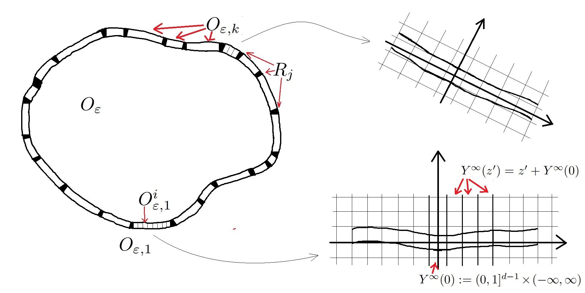
Figure 3: Boundary layer region

From the above decomposition, we have small corners like $R_{j}$ and small cylinders $O_{\varepsilon,k}^{i}$. They have different type geometry properties and some related facts, which will play an important role in later computations.

Remark 4.7 (boundaries of $R_{j}$).

Let $R_{j}$ be given as in $\eqref{eq:4.1}$, and the radial cut-off function $\psi_{\varepsilon}$ be defined as in Lemma 4.6. Then the crucial facts are summarized as follows.

1. In the case of $d=2$ (see Figure 4), we observe that

   • $\nabla\psi_{\varepsilon}=0$ on $\partial R_{j}\cap\partial O_{\varepsilon}$, denoted by $\{(\partial R_{j})^{i}\}_{i=1}^{m_{j}}$ with $m_{j}\in\{1,2\}$;

   • For $\partial R_{j}\cap O_{\varepsilon}$, the boundary must appear in pairs. Moreover, one of them can be derived from the other one by a rational rotation.

2. For the case $d=3$ (see Figure 5), there holds

   • $\nabla\psi_{\varepsilon}=0$ on $\partial R_{j}\cap\partial O_{\varepsilon}$, denoted by $\{(\partial R_{j})^{i}\}_{i=1}^{m_{j}}$ with $m_{j}\in\{1,2,3\}$;

   • For $\partial R_{j}\cap O_{\varepsilon}$, there may exist single boundary surface (dyed by grey color in the small corner drawn in Figure 5), in addition to pairs of surfaces which can be derived from another one among $\partial R_{j}\setminus\{(\partial R_{j})^{i}\}_{i=1}^{m_{j}}$ by one-step translation or rotation (dyed by red color).

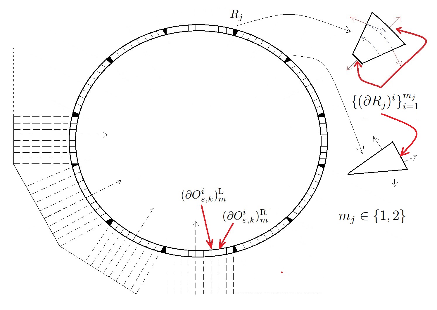
Figure 4: Typical case $d=2$

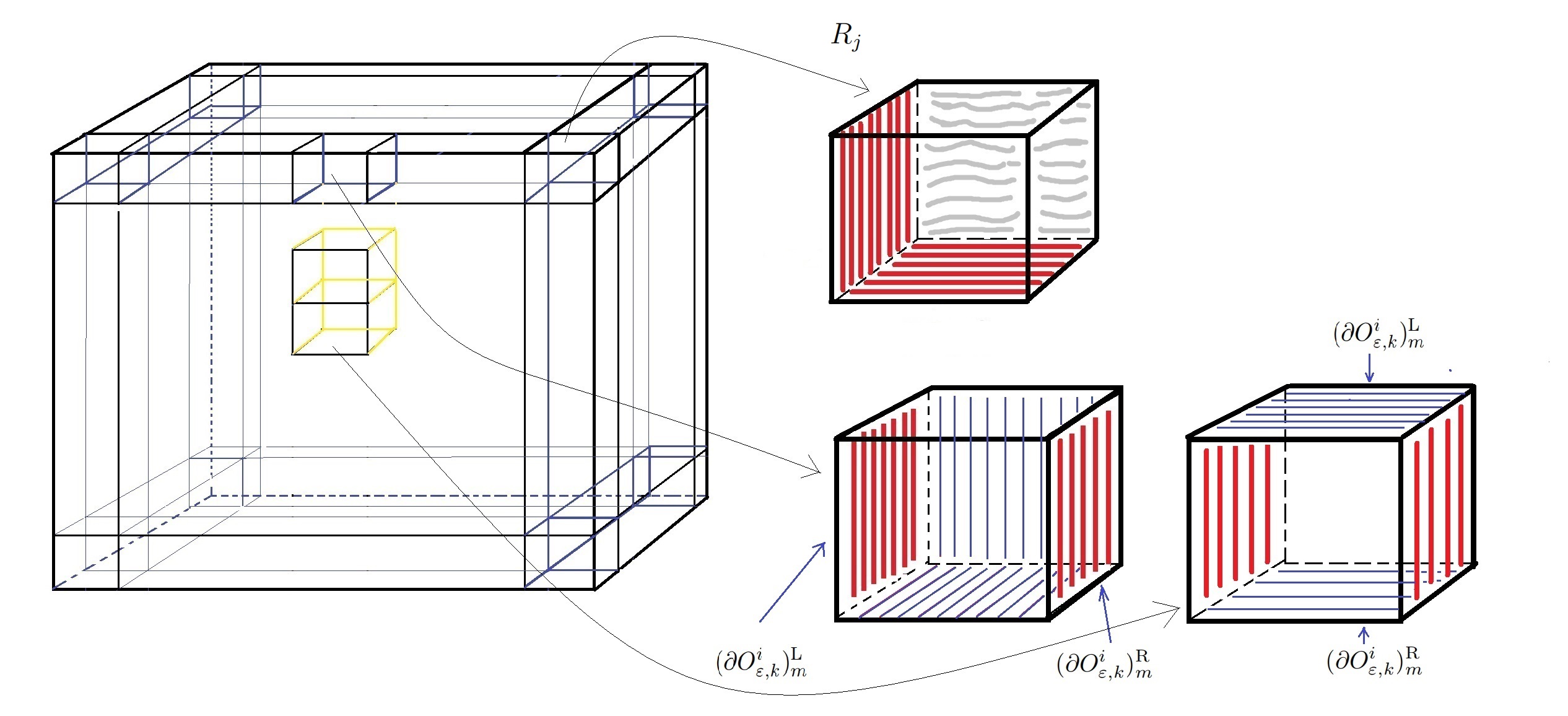
Figure 5: Typical case $d=3$

Remark 4.8 (boundaries of $O_{\varepsilon,k}^{i}$).

Let $O_{\varepsilon,k}^{i}$ be given as in $\eqref{eq:4.2}$ with $k=1,\cdots,K_{0}$ and $i=1,\cdots,N(\varepsilon)$. Then the boundary $\partial O_{\varepsilon,k}^{i}$ consists of two parts: (i) $\partial O_{\varepsilon,k}^{i}\cap\partial O_{\varepsilon}$; (ii) $\partial O_{\varepsilon}^{i}\cap O_{\varepsilon}$. Moreover, there hold the following facts:

• $\nabla\psi_{\varepsilon}=0$ on $\partial O^{i}_{\varepsilon,k}\cap\partial O_{\varepsilon}$;

• the boundaries among $\partial O_{\varepsilon,k}^{i}\cap O_{\varepsilon}$ appear in pairs, denoted by

  $$\partial O_{\varepsilon,k}^{i}\cap O_{\varepsilon}=\bigcup_{m=1}^{d-1}\big{\{}(\partial O_{\varepsilon,k}^{i})_{m}^{\text{L}}\cup(\partial O_{\varepsilon,k}^{i})_{m}^{\text{R}}\big{\}}.$$ (4.16)

  After a $\varepsilon z$-translation or a rational rotation for $(\partial O_{\varepsilon,k}^{i})_{m}^{\text{R}}$, where $z\in\mathbb{Z}^{d}$ and $|z|=1$, its most part can overlap with $(\partial O_{\varepsilon,k}^{i})_{m}^{\text{L}}$. In this regard, we denote this transformation by $\mathrm{T}$, and $\Gamma_{m}^{\text{R}}:=(\partial O_{\varepsilon,k}^{i})_{m}^{\text{R}}(\mathrm{T}\cdot)$. Thus, the intersection part is $(\partial O_{\varepsilon,k}^{i})_{m}^{\text{L}}\cap\Gamma_{m}^{\text{R}}$, and the difference part is $(\partial O_{\varepsilon,k}^{i})_{m}^{\text{L}}\bigtriangleup\Gamma_{m}^{\text{R}}$, which allow us to have

  $$\big{[}(\partial O_{\varepsilon,k}^{i})_{m}^{\text{L}}\cup\Gamma_{m}^{\text{R}}\big{]}=\big{[}(\partial O_{\varepsilon,k}^{i})_{m}^{\text{L}}\cap\Gamma_{m}^{\text{R}}\big{]}\bigcup\big{[}(\partial O_{\varepsilon,k}^{i})_{m}^{\text{L}}\bigtriangleup\Gamma_{m}^{\text{R}}\big{]}.$$ (4.17)

  For the ease of the statement, it is fine to assume $(\partial O_{\varepsilon,k}^{i})_{m}^{\text{L}}\subset\Gamma_{m}^{\text{R}}$ in later computations. On account of the smoothness of $\partial\Omega$, we have the estimate of the difference part:

  $$\big{|}(\partial O_{\varepsilon,k}^{i})_{m}^{\text{L}}\bigtriangleup\Gamma_{m}^{\text{R}}\big{|}\lesssim\varepsilon^{d}.$$ (4.18)

Remark 4.9.

From the above introduction, we can briefly represent the decomposition of $O_{\varepsilon}$ by

$$O_{\varepsilon}=\bigcup_{i}O_{\varepsilon}^{i},$$ (4.19)

where $O_{\varepsilon}^{i}$ could be any element in $\{O_{\varepsilon,k}^{i}\}$ and $\{R_{j}\}$.

Proof of Proposition 4.1

Lemma 4.10 (strong-norm estimates).

Let $\psi_{\varepsilon}$ be the radial cut-off function defined in Lemma 4.6, and $J_{2}$ be given in $\eqref{pde3.8}$. Assume the same conditions as in Proposition 4.1. Then, the first term in the right-hand side of $\eqref{divc2}$ satisfies the following estimate

$$\bigg{(}\int_{0}^{T}\int_{\Omega_{\varepsilon}}\big{|}\frac{\partial J_{2}}{\partial t}\big{|}^{2} \bigg{)}^{1/2}\lesssim\varepsilon^{\frac{1}{2}}\Big{(}\|\partial_{t}\phi\|_{L^{1}(0,T;L^{2}(Y))}+\|\phi(0)\|_{L^{2}(Y_{f})}\Big{)}\|(\nabla G,\varepsilon^{\frac{1}{2}}\nabla^{2}G)\|_{L^{2}(0,T;L^{\infty}(\Omega))}$$ (4.20)

$$+\big{(}\|A^{\prime}\|_{L^{1}(0,T)}+|A(0)|\big{)}\bigg{\{}\varepsilon^{\frac{1}{2}}\|\nabla F\|_{L^{2}(0,T;C^{0}(\bar{\Omega}))}+\|\nabla(G-F)\|_{L^{2}(0,T;L^{2}{(\text{supp}\psi_{\varepsilon})})}\bigg{\}},$$

whose multiplcative constant is independent of $\varepsilon$.

Proof.

By virtue of the equality $\eqref{eq:5.1}$, together with the structure of the effective solution, we can find a cancellation near the boundary w.r.t. outward normal direction, which further provides us with a desired smallness. For the sake of the convenience, we recall the expression of $J_{2}$, as well as the notation $\eqref{notation:4.2}$, and denote it by

$$J_{2} =\nabla\psi_{\varepsilon}\cdot(A\ast G)+\varepsilon\nabla\psi_{\varepsilon}\cdot\big{(}\phi_{\varepsilon}\ast_{2}\partial G\big{)}+\psi_{\varepsilon}\frac{A}{|Y_{f}|}\ast_{2}\partial G+\varepsilon\psi_{\varepsilon}\phi_{\varepsilon}\ast_{3}\partial^{2}G$$ (4.21)

$$:=J_{21}+J_{22}+J_{23}+J_{24},$$

and we complete the whole arguments by three steps, according to the similarity of the computations.

Step 1. We start from the term $\frac{\partial J_{21}}{\partial t}$, and it follows from the equality $\eqref{eq:5.1}$ that

$$\frac{\partial J_{21}}{\partial t}=\nabla\psi_{\varepsilon}\cdot\frac{\partial}{\partial t}(A\ast G) =-|\nabla\psi_{\varepsilon}|\vec{n}\cdot\frac{\partial}{\partial t}(A\ast G)$$ (4.22)

$$=-|\nabla\psi_{\varepsilon}|\vec{n}\cdot\frac{\partial}{\partial t}\big{[}A\ast(G-F)\big{]}-|\nabla\psi_{\varepsilon}|\vec{n}\cdot\frac{\partial}{\partial t}(A\ast F).$$

By noting the fact that $|\nabla\psi_{\varepsilon}|\lesssim\varepsilon^{-1}$ (see Lemma 4.6), there holds

$$\int_{0}^{T}\int_{\Omega_{\varepsilon}}\Big{|}\frac{\partial J_{21}}{\partial t}\Big{|}^{2} \overset{\eqref{f:5.9}}{\lesssim}\varepsilon^{-2}\int_{0}^{T}\int_{O_{\varepsilon}}|\vec{n}\cdot\frac{\partial}{\partial t}(A\ast F)|^{2}+\varepsilon^{-2}\int_{0}^{T}\int_{O_{\varepsilon}}|\vec{n}\cdot\frac{\partial}{\partial t}[A\ast(G-F)]|^{2}.$$ (4.23)

To handle the first term in the right-hand side above, recalling the effective equations $\eqref{pde1.2}$, we have $u_{0}=A\ast F$ with $\vec{n}\cdot u_{0}=0$ on the boundary $\partial\Omega$, whereupon for any $x\in O_{\varepsilon}$ and $t\geq 0$ there holds

$$\vec{n}\cdot\frac{\partial}{\partial t}\big{(}A\ast F\big{)}(x,t)=\vec{n}\cdot\int_{0}^{1}ds\nabla\frac{\partial}{\partial t}\big{(}A\ast F\big{)}(\tilde{x}+s(x-\tilde{x}),t)\cdot(x-\tilde{x}),$$

which further implies

$$\int_{O_{\varepsilon}}\Big{|}\vec{n}\cdot\frac{\partial}{\partial t}\big{(}A\ast F\big{)}(\cdot,t)\Big{|}^{2}\lesssim\varepsilon^{2}\int_{O_{\varepsilon}}\int_{0}^{1}ds\big{|}\nabla\frac{\partial}{\partial t}\big{(}A\ast F\big{)}(\tilde{x}+s(\cdot-\tilde{x}),t)\big{|}^{2}\leq\varepsilon^{2}\int_{\Omega\setminus\Sigma_{2\varepsilon}}|\nabla\frac{\partial}{\partial t}\big{(}A\ast F\big{)}(\cdot,t)|^{2}.$$

Plugging this back into $\eqref{f:5.10}$, and using Young’s inequality we have

$$\quad\int_{0}^{T}\int_{\Omega_{\varepsilon}}\Big{|}\frac{\partial J_{21}}{\partial t}\Big{|}^{2}\lesssim\int_{0}^{T}\int_{\Omega}|\nabla\frac{\partial}{\partial t}(A\ast F)|^{2}+\varepsilon^{-2}\int_{0}^{T}\int_{O_{\varepsilon}}\big{(}|A^{\prime}\ast(G-F)|^{2}+|A(0)(G-F)|^{2}\big{)}$$

$$\lesssim\int_{0}^{T}\int_{\Omega\setminus\Sigma_{2\varepsilon}}\big{(}|A^{\prime}\ast\nabla F|^{2}+|A(0)\nabla F|^{2}\big{)}+\varepsilon^{-2}\int_{0}^{T}\int_{O_{\varepsilon}}\big{(}|A^{\prime}\ast(G-F)|^{2}+|A(0)(G-F)|^{2}\big{)}$$

$$\lesssim\varepsilon\big{(}\|A^{\prime}\|_{L^{1}(0,T)}^{2}+|A(0)|^{2}\big{)}\Big{\{}\|\nabla F\|_{L^{2}(0,T;C(\bar{\Omega}))}^{2}+\varepsilon^{-2}\|G-F\|_{L^{2}(0,T;C(\text{supp}(\psi_{\varepsilon})))}^{2}\Big{\}},$$

and this together with the estimate (Recall the notations $G,F$ in Subsection 1.4.)

$$\|G(\cdot,t)-F(\cdot,t)\|_{C(\text{supp}(\psi_{\varepsilon}))}\lesssim\varepsilon\|\nabla F(\cdot,t)\|_{C(\bar{\Omega})},$$

immediately yields

$$\int_{0}^{T}\int_{\Omega_{\varepsilon}}\Big{|}\frac{\partial J_{21}}{\partial t}\Big{|}^{2}\lesssim\varepsilon\big{(}\|A^{\prime}\|_{L^{1}(0,T)}^{2}+|A(0)|^{2}\big{)}\|\nabla F\|_{L^{2}(0,T;C(\bar{\Omega}))}^{2}.$$ (4.24)

Step 2. We turn to study the term $J_{23}$. Appealing to the fact that $\nabla\cdot u_{0}=A\ast_{2}\partial F=0$ in $\Omega\times(0,T)$, there holds

$$\int_{0}^{T}\int_{\Omega_{\varepsilon}}\Big{|}\frac{\partial J_{23}}{\partial t}\Big{|}^{2} =\int_{0}^{T}\int_{\Omega_{\varepsilon}}\Big{|}\frac{\psi_{\varepsilon}}{|Y_{f}|}\frac{\partial}{\partial t}(A\ast_{2}\partial G)\Big{|}^{2}=\int_{0}^{T}\int_{\Omega_{\varepsilon}}\Big{|}\frac{\psi_{\varepsilon}}{|Y_{f}|}\frac{\partial}{\partial t}[A\ast_{2}\partial(G-F)]\Big{|}^{2}$$

$$=\int_{0}^{T}\int_{\Omega_{\varepsilon}}\Big{|}\frac{\psi_{\varepsilon}}{|Y_{f}|}\Big{(}\big{[}A^{\prime}\ast_{2}\partial(G-F)\big{]}+A(0):\partial(G-F)\Big{)}\Big{|}^{2}.$$

By using Minkowski’s inequality and Young’s inequality, the above equality gives us

$$\int_{0}^{T}\int_{\Omega_{\varepsilon}}\Big{|}\frac{\partial J_{23}}{\partial t}\Big{|}^{2}\lesssim\big{(}\|A^{\prime}\|^{2}_{L^{1}(0,T)}+|A(0)|^{2}\big{)}\|\nabla(G-F)\|^{2}_{L^{2}(0,T;L^{2}{(\text{supp}\psi_{\varepsilon})})}.$$ (4.25)

Step 3. Due to the analogous computations, we consider the terms $J_{22}$ and $J_{24}$ together, and start from the following estimate:

$$\int_{0}^{T}\int_{\Omega_{\varepsilon}}\bigg{|}\frac{\partial J_{22}}{\partial t}+\frac{\partial J_{24}}{\partial t}\bigg{|}^{2} \lesssim\int_{0}^{T}\int_{\Omega_{\varepsilon}}\bigg{|}\varepsilon\nabla\psi_{\varepsilon}(x)\cdot\frac{\partial}{\partial t}(\phi_{\varepsilon}\ast_{2}\partial G)\bigg{|}^{2}+\int_{0}^{T}\int_{\Omega_{\varepsilon}}\bigg{|}\varepsilon\psi_{\varepsilon}\frac{\partial}{\partial t}(\phi_{\varepsilon}\ast_{3}\partial^{2}G)\bigg{|}^{2}$$

$$\lesssim\int_{0}^{T}\int_{O_{\varepsilon}}\big{(}|(\partial_{t}\phi_{\varepsilon})\ast_{2}\partial G|^{2}+|\phi_{\varepsilon}(0):\partial G|^{2}\big{)}$$

$$\qquad+\varepsilon^{2}\int_{0}^{T}\int_{\text{supp}(\psi_{\varepsilon})}\Big{(}|(\partial_{t}\phi_{\varepsilon})\ast_{3}\partial^{2}G|^{2}+|\phi_{\varepsilon}(0)|^{2}|\nabla^{2}G|^{2}\Big{)}.$$

Using Minkowski’s inequality and Young’s inequality we have

$$\int_{0}^{T}dt\int_{O_{\varepsilon}}\Big{(}|(\partial_{t}\phi_{\varepsilon})\ast_{2}\partial G(\cdot,t)|^{2} +|\phi_{\varepsilon}(\cdot,0):\partial G(\cdot,t)|^{2}\Big{)}$$

$$\lesssim\varepsilon\Big{\{}\|\partial_{t}\phi\|^{2}_{L^{1}(0,T;L^{2}(Y_{f}))}+\|\phi(0)\|^{2}_{L^{2}(Y_{f})}\Big{\}}\|\nabla G\|^{2}_{L^{2}(0,T;L^{\infty}(\text{supp}(\psi_{\varepsilon})))},$$

and it similarly follows that

$$\int_{0}^{T}dt\int_{\text{supp}(\psi_{\varepsilon})}\Big{(}|(\partial_{t}\phi_{\varepsilon})\ast_{3}\partial^{2} G(\cdot,t)|^{2}+|\phi_{\varepsilon}(\cdot,0)|^{2}|\nabla^{2}G(\cdot,t)|^{2}\Big{)}$$

$$\lesssim\varepsilon^{2}\Big{\{}\|\partial_{t}\phi\|^{2}_{L^{1}(0,T;L^{2}(Y_{f}))}+\|\phi(0)\|^{2}_{L^{2}(Y_{f})}\Big{\}}\|\nabla^{2}G\|^{2}_{L^{2}(0,T;L^{\infty}(\text{supp}(\psi_{\varepsilon})))}.$$

Thus, combining the three estimates above, we derive that

$$\quad\int_{0}^{T}\int_{\Omega_{\varepsilon}}\Big{|}\frac{\partial J_{22}}{\partial t}+\frac{\partial J_{24}}{\partial t}\Big{|}^{2}$$ (4.26)

$$\lesssim\varepsilon\Big{(}\|\partial_{t}\phi\|^{2}_{L^{1}(0,T;L^{2}(Y_{f}))}+\|\phi(0)\|^{2}_{L^{2}(Y_{f})}\Big{)}\|(\nabla G,\varepsilon^{\frac{1}{2}}\nabla^{2}G)\|^{2}_{L^{2}(0,T;L^{\infty}(\text{supp}(\psi_{\varepsilon})))}.$$

Consequently, the desired estimate $\eqref{pri:5.1}$ follows from the combination of $\eqref{f:5.11}$, $\eqref{*xi2}$, $\eqref{*xi3}$ and $\eqref{*xi1}$. This ends the proof. ∎

Lemma 4.11 (weak-norm estimates).

Let $J_{1}$ be given in $\eqref{pde3.8}$. Suppose that $O_{\varepsilon}$ is decomposed as in Subsection 4.2, and the decomposed small region $O_{\varepsilon}^{i}$ has been defined as in Remark 4.9. Then there holds the estimate

$$\bigg{(}\int_{0}^{T}\int_{\Omega_{\varepsilon}}\Big{|}\sum_{i}(\mathchoice{{\vbox{\hbox{$\textstyle-$}}\kern-4.86108pt}}{{\vbox{\hbox{$\scriptstyle-$}}\kern-3.25pt}}{{\vbox{\hbox{$\scriptscriptstyle-$}}\kern-2.29166pt}}{{\vbox{\hbox{$\scriptscriptstyle-$}}\kern-1.875pt}}\!\int_{O_{\varepsilon}^{i}}\frac{\partial J_{1}}{\partial t})1_{O_{\varepsilon}^{i}}\Big{|}^{2}\bigg{)}^{1/2}$$ (4.27)

$$\lesssim \varepsilon^{\frac{1}{2}}\|(G,\nabla G)\|_{L^{2}(0,T;L^{\infty}(\text{supp}(\psi_{\varepsilon})))}\bigg{\{}\|\partial_{t}\Phi\|_{L^{1}(0,T;L^{\infty}(Y))}+\|\Phi(0)\|_{L^{\infty}(Y)}\bigg{\}},$$

where the up to constant depends on $d$ and the character of $\Omega$, but independent of $\varepsilon$.

Proof.

According to Remark 4.9, $O_{\varepsilon}^{i}$ could be any element in $\{O_{\varepsilon,k}^{i}\}$ and $\{R_{j}\}$. For simplicity, if $O_{\varepsilon}^{i}$ is an element of $\{O_{\varepsilon,k}^{i}\}$, we still denote it by itself. Otherwise, we adopt the notation $R_{j}$. Therefore, it suffices to estimate the left-hand side below

$$\int_{0}^{T}\int_{\Omega_{\varepsilon}}\Big{|}\sum_{i}(\mathchoice{{\vbox{\hbox{$\textstyle-$}}\kern-4.86108pt}}{{\vbox{\hbox{$\scriptstyle-$}}\kern-3.25pt}}{{\vbox{\hbox{$\scriptscriptstyle-$}}\kern-2.29166pt}}{{\vbox{\hbox{$\scriptscriptstyle-$}}\kern-1.875pt}}\!\int_{O_{\varepsilon}^{i}}\frac{\partial J_{1}}{\partial t})1_{O_{\varepsilon}^{i}}\Big{|}^{2}\leq\int_{0}^{T}\int_{\Omega_{\varepsilon}}\Big{|}\sum_{i}^{N(\varepsilon)}(\mathchoice{{\vbox{\hbox{$\textstyle-$}}\kern-4.86108pt}}{{\vbox{\hbox{$\scriptstyle-$}}\kern-3.25pt}}{{\vbox{\hbox{$\scriptscriptstyle-$}}\kern-2.29166pt}}{{\vbox{\hbox{$\scriptscriptstyle-$}}\kern-1.875pt}}\!\int_{O_{\varepsilon}^{i}}\frac{\partial J_{1}}{\partial t})1_{O_{\varepsilon}^{i}}+\sum\limits_{j=1}^{K_{0}}(\mathchoice{{\vbox{\hbox{$\textstyle-$}}\kern-4.86108pt}}{{\vbox{\hbox{$\scriptstyle-$}}\kern-3.25pt}}{{\vbox{\hbox{$\scriptscriptstyle-$}}\kern-2.29166pt}}{{\vbox{\hbox{$\scriptscriptstyle-$}}\kern-1.875pt}}\!\int_{R_{j}}\frac{\partial J_{1}}{\partial t})1_{R_{j}}\Big{|}^{2},$$ (4.28)

where $K_{0}$ is defined as the same as in $\eqref{eq:4.1}$, and $N(\varepsilon)=\sum_{k=1}^{K_{0}}N_{k}(\varepsilon)$. For each of the quantities $\{N_{k}(\varepsilon)\}$, it is similar to the counterpart of $\eqref{eq:4.2}$.

The proof totally consists three parts. Under the preconditions $\eqref{*pde4.8}$ and $\eqref{*pde4.15}$, the first part is devoted to giving the desired estimate $\eqref{pri:5.0}$. As stated in the estimate $\eqref{*pde4.1}$, due to the decomposition introduced in Subsection 4.2, the second part is to show $\eqref{*pde4.8}$, and third one is for $\eqref{*pde4.15}$.

Part 1. For the ease of the statement, we firstly introduce the following notation

$$Q_{1}(t) :=\int_{0}^{t}ds\|\partial_{t}\Phi(t-s)\|_{L^{\infty}(Y)}\|\nabla G(s)\|_{L^{\infty}(\text{supp}(\psi_{\varepsilon}))}+\|\Phi(0)\|_{L^{\infty}(Y)}\|\nabla G(t)\|_{L^{\infty}(\text{supp}(\psi_{\varepsilon}))};$$ (4.29)

$$Q_{2}(t) :=\int_{0}^{t}ds\|\partial_{t}\Phi(t-s)\|_{L^{\infty}(Y)}\|G(s)\|_{L^{\infty}(\text{supp}(\psi_{\varepsilon}))}(t)+\|\Phi(0)\|_{L^{\infty}(Y)}\|G(t)\|_{L^{\infty}(\text{supp}(\psi_{\varepsilon}))}.$$

The second part is devoted to showing the estimates for the regular decomposition part, i.e.,

$$\bigg{|}\mathchoice{{\vbox{\hbox{$\textstyle-$}}\kern-4.86108pt}}{{\vbox{\hbox{$\scriptstyle-$}}\kern-3.25pt}}{{\vbox{\hbox{$\scriptscriptstyle-$}}\kern-2.29166pt}}{{\vbox{\hbox{$\scriptscriptstyle-$}}\kern-1.875pt}}\!\int_{O_{\varepsilon}^{i}}\frac{\partial J_{1}}{\partial t}(\cdot,t)\bigg{|} \lesssim Q_{1}(t)+Q_{2}(t),$$ (4.30)

and then we are also interested in the estimates on the irregular part:

$$\Big{|}\mathchoice{{\vbox{\hbox{$\textstyle-$}}\kern-4.86108pt}}{{\vbox{\hbox{$\scriptstyle-$}}\kern-3.25pt}}{{\vbox{\hbox{$\scriptscriptstyle-$}}\kern-2.29166pt}}{{\vbox{\hbox{$\scriptscriptstyle-$}}\kern-1.875pt}}\!\int_{R_{j}}\frac{\partial J_{1}}{\partial t}(\cdot,t)\Big{|}\lesssim\left\{\begin{aligned} &Q_{1}(t),&&d=2;\\ &Q_{1}(t)+\varepsilon^{-1}Q_{2}(t),&&d=3,\end{aligned}\right.$$ (4.31)

where the up to constant is independent of $i,j$ and $t$. Let the left-hand side of $\eqref{*pde4.1}$ be denoted by $L$. Once we established the estimates $\eqref{*pde4.8}$ and $\eqref{*pde4.15}$, plugging them into the right-hand side of $\eqref{*pde4.1}$, we would have

$$L\leq\int_{0}^{T}dt\int_{\Omega_{\varepsilon}}1_{O_{\varepsilon}}\big{[}Q_{1}(t)+Q_{2}(t)\big{]}^{2}+(d-2)\sum_{j=1}^{K_{0}}\varepsilon^{-2}\int_{0}^{T}dt\int_{\Omega_{\varepsilon}}1_{R_{j}}\big{[}Q_{2}(t)\big{]}^{2}.$$

From the Fubini theorem, Young’s inequality and the fact that $|O_{\varepsilon}|=O(\varepsilon)$ with $|R_{j}|=O(\varepsilon^{d})$ (see $\eqref{eq:4.1}$), it follows that

$$L \lesssim|O_{\varepsilon}|\int_{0}^{T}dt\big{[}Q_{1}(t)+Q_{2}(t)\big{]}^{2}+(d-2)\varepsilon^{d-2}\int_{0}^{T}dt\big{[}Q_{2}(t)\big{]}^{2}$$

$$\lesssim\varepsilon\bigg{\{}\|\partial_{t}\Phi\|_{L^{1}(0,T;L^{\infty}(Y))}^{2}\|\nabla G\|_{L^{2}(0,T;L^{\infty}(\text{supp}(\psi_{\varepsilon})))}^{2}+\|\Phi(0)\|_{L^{\infty}(Y)}^{2}\|\nabla G\|_{L^{2}(0,T;L^{\infty}(\text{supp}(\psi_{\varepsilon})))}^{2}\bigg{\}}$$

$$+\varepsilon\bigg{\{}\|\partial_{t}\Phi\|_{L^{1}(0,T;L^{\infty}(Y))}^{2}\|G\|_{L^{2}(0,T;L^{\infty}(\text{supp}(\psi_{\varepsilon})))}^{2}+\|\Phi(0)\|_{L^{\infty}(Y)}^{2}\|G\|_{L^{2}(0,T;L^{\infty}(\text{supp}(\psi_{\varepsilon})))}^{2}\bigg{\}}.$$

This gives us the desired estimate $\eqref{pri:5.0}$.

Part 2. We now address the estimate $\eqref{*pde4.8}$. On account of the antisymmetric property of flux corrector $\Phi$ in Proposition 2.1, integrating by parts we obtain that

$$\int_{O_{\varepsilon}^{i}}\frac{\partial J_{1}}{\partial t}(\cdot,t) =\int_{O_{\varepsilon}^{i}}\frac{\partial}{\partial t}[(W^{\varepsilon}-A)\ast G](\cdot,t)\cdot\nabla\psi_{\varepsilon}=\int_{O_{\varepsilon}^{i}}\frac{\partial}{\partial t}\big{[}(\nabla\cdot\Phi)^{\varepsilon}\ast G\big{]}(\cdot,t)\cdot\nabla\psi_{\varepsilon}$$ (4.32)

$$\overset{\eqref{anti-sym}}{=}-\varepsilon\int_{O_{\varepsilon}^{i}}\frac{\partial}{\partial t}\big{[}\Phi^{\varepsilon}\ast_{2}\partial G\big{]}(\cdot,t)\cdot\nabla\psi_{\varepsilon}+\varepsilon\int_{\partial O_{\varepsilon}^{i}}dS\frac{\partial}{\partial t}\big{[}\Phi^{\varepsilon}\ast_{3}(G\otimes\nabla\psi_{\varepsilon}\otimes\vec{n}_{s})\big{]}(\cdot,t)$$

$$: =E_{1}(t)+E_{2}(t),$$

in which $\vec{n}_{s}$ is the unit outward normal vector of the boundary $\partial O_{\varepsilon}^{i}$.

We start from estimating the first term $E_{1}(t)$. Recalling the properties of the cut-off function $\psi_{\varepsilon}$ stated in Lemma 4.6, a direct computation leads to

$$|E_{1}(t)| \lesssim\int_{O_{\varepsilon}^{i}}\bigg{|}\frac{\partial}{\partial t}[\Phi^{\varepsilon}\ast_{2}\partial G](\cdot,t)\bigg{|}=\int_{O_{\varepsilon}^{i}}\bigg{|}(\partial_{t}\Phi^{\varepsilon}\ast_{2}\partial G)(\cdot,t)+\Phi^{\varepsilon}(\cdot,0):\partial G(\cdot,t)\bigg{|}$$

$$\leq\int_{O_{\varepsilon}^{i}}\big{|}\partial_{t}\Phi^{\varepsilon}\ast_{2}\partial G\big{|}(\cdot,t)+|O_{\varepsilon}^{i}|\|\Phi(0)\|_{L^{\infty}(Y)}\|\nabla G(t)\|_{L^{\infty}(O_{\varepsilon})}.$$

This together with the estimate (Recall the definition of the notation $\eqref{notation:4.2}$.)

$$\int_{O_{\varepsilon}^{i}}\big{|}\partial_{t}\Phi^{\varepsilon}\ast_{2}\partial G\big{|}(\cdot,t)\leq\int_{0}^{t}ds\int_{O_{\varepsilon}^{i}}\big{|}\partial_{s}\Phi^{\varepsilon}(\cdot,s):\partial G(\cdot,t-s)\big{|}\leq|O_{\varepsilon}^{i}|\Big{(}\|\partial_{t}\Phi\|_{L^{\infty}(Y)}\ast_{2}\|\partial G\|_{L^{\infty}(O_{\varepsilon})}\Big{)}(t)$$

finally gives us

$$|E_{1}(t)|\lesssim|O_{\varepsilon}^{i}|\bigg{\{}\|\partial_{t}\Phi\|_{L^{\infty}(Y)}\ast_{2}\|\partial G\|_{L^{\infty}(O_{\varepsilon})}(t)+\|\Phi(0)\|_{L^{\infty}(Y)}\|\nabla G(t)\|_{L^{\infty}(O_{\varepsilon})}\bigg{\}}.$$ (4.33)

Then we turn to estimate the second term $E_{2}$ in $\eqref{*pde4.9}$, which involves more geometrical details on $\partial O_{\varepsilon}^{i}$. From (a) in Remark 4.8 and the construction of $\psi_{\varepsilon}$ given in Lemma 4.6, it concludes that $\nabla\psi_{\varepsilon}(x)=0$ on $\partial O_{\varepsilon}^{i}\cap\partial O_{\varepsilon}$. Thus, to complete the estimate of $E_{2}$, it suffices to focus ourselves on the case $\partial O_{\varepsilon}^{i}\cap O_{\varepsilon}$. As shown in $\eqref{notation:4.3}$, omitting its subscript $k$, we impose the notation to represent the lateral boundaries, which actually appear in pairs

$$\partial O_{\varepsilon}^{i}\cap O_{\varepsilon}=\bigcup_{m=1}^{d-1}\big{\{}(\partial O_{\varepsilon}^{i})_{m}^{\text{L}}\cup(\partial O_{\varepsilon}^{i})_{m}^{\text{R}}\big{\}},$$

where $\big{\{}(\partial O_{\varepsilon}^{i})_{m}^{\text{L}}\cup(\partial O_{\varepsilon}^{i})_{m}^{\text{R}}\big{\}}$ is known as one pair of the lateral boundaries. Therefore, by virtue of the notation defined above, we can rewrite $E_{2}$ as

$$E_{2}(t)=\varepsilon\sum_{m=1}^{d-1}\bigg{\{}\int_{(\partial O_{\varepsilon}^{i})_{m}^{\text{L}}}+\int_{(\partial O_{\varepsilon}^{i})_{m}^{\text{R}}}\bigg{\}}dS\frac{\partial}{\partial t}\big{[}\Phi^{\varepsilon}\ast_{3}(G\otimes\nabla\psi_{\varepsilon}\otimes\vec{n}_{s})\big{]}(\cdot,t):=\varepsilon\sum_{m=1}^{d-1}E_{2}^{m}(t),$$

which is reduced to study the quantity $E_{2}^{m}$ for $m=1,\cdots,d-1$.

For any fixed $i$ and $m$, denoted the related $\varepsilon z$-translation or rational rotation transformation by $\mathrm{T}^{i}_{m}$, it follows from the equality $\eqref{eq:4.3}$ together with the notation therein that

$$\Gamma_{m}^{\text{R}}=(\partial O_{\varepsilon}^{i})_{m}^{\text{L}}\bigcup\big{[}(\Gamma_{m}^{\text{R}}\setminus(\partial O_{\varepsilon}^{i})_{m}^{\text{L}}\big{]}.$$ (4.34)

According to the periodicity of flux corrector, we therefore have $\Phi^{\varepsilon}=\Phi^{\varepsilon}((\mathrm{T}^{i}_{m})^{-1}\cdot)$. Moreover, we note that the unit outward normal vector $\vec{n}_{s}$ of $\partial O_{\varepsilon}^{i}$ takes the opposite direction on $(\partial O_{\varepsilon}^{i})_{m}^{\text{L}}$ and $(\partial O_{\varepsilon}^{i})_{m}^{\text{R}}$. On account of the above two facts, we can derive that

$$E_{2}^{m}(t) =\int_{(\partial O_{\varepsilon}^{i})_{m}^{\text{L}}}dS\frac{\partial}{\partial t}\bigg{\{}\Phi^{\varepsilon}\ast_{3}\Big{[}\big{(}G-G((\mathrm{T}^{i}_{m})^{-1}\cdot)\big{)}\otimes\nabla\psi_{\varepsilon}\otimes\vec{n}_{s}\Big{]}(\cdot,t)\bigg{\}}$$ (4.35)

$$+\int_{(\partial O_{\varepsilon}^{i})_{m}^{\text{L}}}dS\frac{\partial}{\partial t}\bigg{\{}\Phi^{\varepsilon}\ast_{3}\Big{[}G((\mathrm{T}^{i}_{m})^{-1}\cdot)\otimes\big{(}\nabla\psi_{\varepsilon}-\nabla\psi_{\varepsilon}((\mathrm{T}^{i}_{m})^{-1}\cdot)\big{)}\otimes\vec{n}_{s}\Big{]}(\cdot,t)\bigg{\}}$$

$$-\int_{\Gamma_{m}^{\text{R}}\setminus(\partial O_{\varepsilon}^{i})_{m}^{\text{L}}}dS\frac{\partial}{\partial t}\bigg{\{}\Phi^{\varepsilon}\ast_{3}\Big{[}G\otimes\nabla\psi_{\varepsilon}\otimes\vec{n}_{s}\Big{]}((\mathrm{T}^{i}_{m})^{-1}\cdot,t)\bigg{\}}:=E_{2,1}^{m}(t)+E_{2,2}^{m}(t)+E_{2,3}^{m}(t).$$

Due to $\eqref{eq:5.2}$, it is not hard to observe that the distance function satisfies $\text{dist}(\cdot,\partial\Omega)=\text{dist}((\mathrm{T}^{i}_{m})^{-1}\cdot,\partial\Omega)$ on $(\partial O_{\varepsilon}^{i})_{m}^{\text{L}}$, and this together with Lemma 4.6 further leads to $\nabla\psi_{\varepsilon}-\nabla\psi_{\varepsilon}((\mathrm{T}^{i}_{m})^{-1}\cdot)=0$ on $(\partial O_{\varepsilon}^{i})_{m}^{\text{L}}$, whereupon the second term $E_{2,2}^{m}$ vanishes.

We then turn to the last term $E_{2,3}^{m}$ of $\eqref{*pde3.18}$. In view of $\eqref{eq:4.4}$ and Fubini’s theorem, we simply obtain that

$$|E_{2,3}^{m}(t)|\lesssim\varepsilon^{d}\Big{\{}\|\partial_{t}\Phi\|_{L^{\infty}(Y)}\ast\|G\|_{L^{\infty}(\text{supp}(\psi_{\varepsilon}))}(t)+\|\Phi(0)\|_{L^{\infty}(Y)}\|G(t)\|_{L^{\infty}(\text{supp}(\psi_{\varepsilon}))}\Big{\}}.$$ (4.36)

We now continue to study the term $E_{2,1}^{m}$ in the right-hand side of $\eqref{*pde3.18}$ and start by taking the derivative of $t$ into the convolution, (we denote the exponent of $\vec{n}_{s}$ by $\vec{n}_{s}^{\alpha}$ with $\alpha=1,\cdots,d$.)

$$|E_{2,1}^{m}(t)| \leq\int_{(\partial O_{\varepsilon}^{i})_{m}^{\text{L}}}dS\bigg{|}\int_{0}^{t}ds\partial_{t}\Phi_{k\alpha,\beta}^{\varepsilon}(\cdot,t-s)\big{(}G_{\beta}(\cdot,s)-G_{\beta}((\mathrm{T}^{i}_{m})^{-1}\cdot,s)\big{)}\nabla_{k}\psi_{\varepsilon}n_{s}^{\alpha}\bigg{|}$$ (4.37)

$$+\int_{(\partial O_{\varepsilon}^{i})_{m}^{\text{L}}}dS\bigg{|}\Phi_{k\alpha,\beta}^{\varepsilon}(\cdot,0)\big{(}G_{\beta}(\cdot,t)-G_{\beta}((\mathrm{T}^{i}_{m})^{-1}\cdot,t)\big{)}\nabla_{k}\psi_{\varepsilon}n_{s}^{\alpha}\bigg{|}.$$

From the differential mean value theorem, it follows that

$$\sup_{x\in O_{\varepsilon}}|G(x,t)-G((\mathrm{T}^{i}_{m})^{-1}x,t)|\lesssim\varepsilon\|\nabla G(t)\|_{L^{\infty}(O_{\varepsilon})}.$$

Plugging this estimate back into $\eqref{f:5.1}$, by using Fubini’s theorem again, we have

$$|E_{2,1}^{m}(t)| \lesssim\varepsilon|(\partial O_{\varepsilon}^{i})_{m}^{\text{L}}|\bigg{\{}\int_{0}^{t}ds\|\partial_{t}\Phi(t-s)\|_{L^{\infty}(Y)}\|\nabla G(s)\|_{L^{\infty}(O_{\varepsilon})}+\|\Phi(0)\|_{L^{\infty}(Y)}\|\nabla G(t)\|_{L^{\infty}(O_{\varepsilon})}\bigg{\}},$$

and this together with $\eqref{f:5.14}$ and $\eqref{*pde3.18}$ implies that (Recall the notation $\eqref{notation:5.1}$ and $|O_{\varepsilon}^{i}|\sim\varepsilon|\partial O_{\varepsilon}^{i}|=O(\varepsilon^{d})$.)

$$|E_{2}^{m}(t)|\lesssim|O_{\varepsilon}^{i}|\Big{\{}Q_{1}(t)+Q_{2}(t)\Big{\}}.$$ (4.38)

As a result, by noting the relationship $E_{2}(t):=\varepsilon\sum_{m=1}^{d-1}E_{2}^{m}(t)$, we obtain

$$|E_{2}(t)|\overset{\eqref{f:5.2}}{\lesssim}|O_{\varepsilon}^{i}|\Big{\{}Q_{1}(t)+Q_{2}(t)\Big{\}},$$

which combines the estimates $\eqref{*pde4.9}$ and $\eqref{*pde3.19}$ to give us the stated estimate $\eqref{*pde4.8}$.

Part 3. This part is devoted to showing the estimate $\eqref{*pde4.15}$. Using the same idea as given for $\eqref{*pde4.9}$ in Part 2, appealing to the antisymmetric property of flux corrector $\Phi$ again (see Proposition 2.1), we have

$$\int_{R_{j}}\frac{\partial J_{1}}{\partial t}(\cdot,t) \overset{\eqref{anti-sym}}{=}-\varepsilon\int_{R_{j}}\frac{\partial}{\partial t}\big{[}\Phi^{\varepsilon}\ast_{2}\partial G\big{]}(\cdot,t)\cdot\nabla\psi_{\varepsilon}+\varepsilon\int_{\partial R_{j}}dS\frac{\partial}{\partial t}\big{[}\Phi^{\varepsilon}\ast_{3}(G\otimes\nabla\psi_{\varepsilon}\otimes\vec{n}_{s})\big{]}(\cdot,t)$$ (4.39)

$$: =E_{3}(t)+E_{4}(t),$$

We can deal with the term $E_{3}$ as we did for $E_{1}$ in $\eqref{*pde3.19}$, and it follows that

$$|E_{3}(t)|\lesssim|R_{j}|\bigg{\{}\|\Phi(0)\|_{L^{\infty}(Y)}\|\nabla G(t)\|_{L^{\infty}(O_{\varepsilon})}+\|\partial_{t}\Phi\|_{L^{\infty}(Y)}\ast_{2}\|\partial G\|_{L^{\infty}(O_{\varepsilon})}(t)\bigg{\}}.$$ (4.40)

The main difference between the terms $E_{4}$ and $E_{2}$ is that the geometry of $R_{j}$ is not as the same as that of $O^{i}_{\varepsilon}$. The main challenge is that we have to find a “smallness” in the same level but from the different geometry facts (1.2) and (2.2) in Remark 4.7. The ideas are following: (I) using dimensional condition to increase a “smallness” for the case $d=3$; (II) employing the invariant property of flux corrector in terms of rotation (requiring all its components to be rational number) for the case $d=2$.

We firstly handle the case $d=3$, and start from a direct computation.

$$|E_{4}(t)|\lesssim|\partial R_{j}|\bigg{\{}\|\Phi(0)\|_{L^{\infty}(Y)}\|G(t)\|_{L^{\infty}(O_{\varepsilon})}+\|\partial_{t}\Phi\|_{L^{\infty}(Y)}\ast\|G\|_{L^{\infty}(O_{\varepsilon})}(t)\bigg{\}}.$$ (4.41)

Then combining the estimates $\eqref{f:5.3}$, $\eqref{f:5.4}$ and $\eqref{f:5.5}$, we obtain

$$\Big{|}\mathchoice{{\vbox{\hbox{$\textstyle-$}}\kern-4.86108pt}}{{\vbox{\hbox{$\scriptstyle-$}}\kern-3.25pt}}{{\vbox{\hbox{$\scriptscriptstyle-$}}\kern-2.29166pt}}{{\vbox{\hbox{$\scriptscriptstyle-$}}\kern-1.875pt}}\!\int_{R_{j}}\frac{\partial J_{1}}{\partial t}(\cdot,t)\Big{|} \lesssim\|\Phi(0)\|_{L^{\infty}(Y)}\Big{\{}\varepsilon^{-1}\|G(t)\|_{L^{\infty}(O_{\varepsilon})}+\|\nabla G(t)\|_{L^{\infty}(O_{\varepsilon})}\Big{\}}$$

$$+\varepsilon^{-1}\|\partial_{t}\Phi\|_{L^{\infty}(Y)}\ast\|G\|_{L^{\infty}(O_{\varepsilon})}(t)+\int_{0}^{t}ds\|\partial_{t}\Phi(t-s)\|_{L^{\infty}(Y)}\|\nabla G(s)\|_{L^{\infty}(O_{\varepsilon})},$$

and this gives the second line of $\eqref{*pde4.15}$.

We now turn to deal with the case $d=2$. By (2.1) and (2,2) in Remark 4.7, it is known that the boundaries of $R_{j}$ consist of two parts, and we denote by $\partial R_{j}:=\{(\partial R_{j})^{i}\}_{i=1}^{m_{j}}\cup(\partial R_{j})^{\text{L}}\cup(\partial R_{j})^{\text{R}}$, where we can obtain $(\partial R_{j})^{\text{L}}$ by rotating $(\partial R_{j})^{\text{R}}$ by $\theta$ anticlockwise (see Figure 4). This rational rotation is denoted by

$$\text{R}_{\theta}=\left(\begin{matrix}\cos\theta&-\sin\theta\\ \sin\theta&\cos\theta\end{matrix}\right),$$

and from the periodicity it follows that

$$\Psi^{\varepsilon}=\Psi^{\varepsilon}(\text{R}_{\theta}\cdot).$$ (4.42)

Moreover, we observe that there holds $\text{dist}(x,\partial\Omega)=\text{dist}(\text{R}_{\theta}^{-1}x,\partial\Omega)$ for any $x\in(\partial R_{j})^{\text{L}}$, and therefore by Lemma 4.6 we have

$$\nabla\psi_{\varepsilon}-\nabla\psi_{\varepsilon}(\text{R}_{\theta}^{-1}\cdot)=0\quad\text{on}\quad(\partial R_{j})^{\text{L}}.$$ (4.43)

By the analogous computation as in $\eqref{*pde3.18}$, the equality $\eqref{f:5.6}$, and the fact that after counterclockwise rotation the outward normal direction of side $(\partial R_{j})^{\text{R}}$ is opposite to that of side $(\partial R_{j})^{\text{L}}$, we obtain that

$$E_{4}(t) =\varepsilon\int_{(\partial R_{j})^{\text{L}}}dS\frac{\partial}{\partial t}\bigg{\{}\Phi^{\varepsilon}\ast_{3}\Big{[}\big{(}G-G(\text{R}_{\theta}^{-1}\cdot)\big{)}\otimes\nabla\psi_{\varepsilon}\otimes\vec{n}_{s}\Big{]}(\cdot,t)\bigg{\}}$$

$$+\varepsilon\int_{(\partial R_{j})^{\text{L}}}dS\frac{\partial}{\partial t}\bigg{\{}\Phi^{\varepsilon}\ast_{3}\Big{[}G(\text{R}_{\theta}^{-1}\cdot)\otimes\big{(}\nabla\psi_{\varepsilon}-\nabla\psi_{\varepsilon}(\text{R}_{\theta}^{-1}\cdot)\big{)}\otimes\vec{n}_{s}\Big{]}(\cdot,t)\bigg{\}},$$

which coupled with (4.43) implies

$$|E_{4}(t)|\leq|R_{j}|\bigg{\{}\int_{0}^{t}ds\|\partial_{t}\Phi(t-s)\|_{L^{\infty}(Y)}\|\nabla G(s)\|_{L^{\infty}(O_{\varepsilon})}+\|\Phi(0)\|_{L^{\infty}(Y)}\|\nabla G(t)\|_{L^{\infty}(O_{\varepsilon})}\bigg{\}}.$$ (4.44)

In such the case, collecting the estimates $\eqref{f:5.3}$, $\eqref{f:5.4}$ and $\eqref{f:5.8}$ we arrive at

$$\Big{|}\mathchoice{{\vbox{\hbox{$\textstyle-$}}\kern-4.86108pt}}{{\vbox{\hbox{$\scriptstyle-$}}\kern-3.25pt}}{{\vbox{\hbox{$\scriptscriptstyle-$}}\kern-2.29166pt}}{{\vbox{\hbox{$\scriptscriptstyle-$}}\kern-1.875pt}}\!\int_{R_{j}}\frac{\partial J_{1}}{\partial t}(\cdot,t)\Big{|}\lesssim\int_{0}^{t}ds\|\partial_{t}\Phi(t-s)\|_{L^{\infty}(Y)}\|\nabla G(s)\|_{L^{\infty}(O_{\varepsilon})}+\|\Phi(0)\|_{L^{\infty}(Y)}\|\nabla G(t)\|_{L^{\infty}(O_{\varepsilon})},$$

which consequently implies the first line of $\eqref{*pde4.15}$. This ends the whole proof. ∎

Lemma 4.12 (existences).

There exists at least one weak solution for (4.1) and (4.3), respectively.

Proof.

The existence of weak solution for (4.1) and (4.3) follows from compatibility condition for divergence operator and it’s obvious for (4.3). Recalling the definition of $J_{1}$ and $J_{2}$ in (1.19), and the fact

$$\nabla\cdot\bigg{\{}\psi_{\varepsilon}[W^{\varepsilon}\ast G+\varepsilon\phi^{\varepsilon}_{k,j}\ast\nabla_{k}G_{j}]\bigg{\}}=J_{1}+J_{2},$$

it follows that

$$\int_{\Omega_{\varepsilon}}(J_{1}+J_{2})(\cdot,t)=\int_{\Omega_{\varepsilon}}\nabla\cdot\bigg{\{}\psi_{\varepsilon}[W^{\varepsilon}\ast G+\varepsilon\phi^{\varepsilon}\ast\nabla G]\bigg{\}}(\cdot,t)=\int_{\partial\Omega_{\varepsilon}}dS\vec{n}\cdot\bigg{\{}\psi_{\varepsilon}[W^{\varepsilon}\ast G+\varepsilon\phi^{\varepsilon}\ast\nabla G]\bigg{\}}(\cdot,t)=0.$$

Therefore, due to the fact that supp$(J_{1})=O_{\varepsilon}=\sum\limits_{i}O_{\varepsilon}^{i}$ (see Remark 4.9), there holds

$$\int_{\Omega_{\varepsilon}}\Big{[}J_{2}+\sum_{i}(\mathchoice{{\vbox{\hbox{$\textstyle-$}}\kern-4.86108pt}}{{\vbox{\hbox{$\scriptstyle-$}}\kern-3.25pt}}{{\vbox{\hbox{$\scriptscriptstyle-$}}\kern-2.29166pt}}{{\vbox{\hbox{$\scriptscriptstyle-$}}\kern-1.875pt}}\!\int_{O_{\varepsilon}^{i}}J_{1})1_{O_{\varepsilon}^{i}}\Big{]}(\cdot,t)=\int_{\Omega_{\varepsilon}}\big{(}J_{1}+J_{2}\big{)}(\cdot,t)=0.$$

Consequently, we have

$$\int_{\Omega_{\varepsilon}}\Big{[}\frac{\partial J_{2}}{\partial t}+\sum_{i}(\mathchoice{{\vbox{\hbox{$\textstyle-$}}\kern-4.86108pt}}{{\vbox{\hbox{$\scriptstyle-$}}\kern-3.25pt}}{{\vbox{\hbox{$\scriptscriptstyle-$}}\kern-2.29166pt}}{{\vbox{\hbox{$\scriptscriptstyle-$}}\kern-1.875pt}}\!\int_{O_{\varepsilon}^{i}}\frac{\partial J_{1}}{\partial t})1_{O_{\varepsilon}^{i}}\Big{]}(\cdot,t)=\int_{\Omega_{\varepsilon}}\partial_{t}\big{(}J_{1}+J_{2}\big{)}(\cdot,t)=0.$$

This is the compatibility condition for (4.1). ∎

The proof of Proposition 4.1. The existence of the solution of $\eqref{divc2}$ has been established in Lemma 4.12, while the main job is to show the estimate $\eqref{pri:4.1}$. To do so, applying Theorem 4.4 to the solution of the equations $\eqref{divc2}$, we have

$$\|\xi\|_{L^{2}(\Omega_{\varepsilon,T})}\lesssim\varepsilon\|\nabla\xi\|_{L^{2}(\Omega_{\varepsilon,T})} \overset{\eqref{pde3.21}}{\lesssim}\big{\|}\frac{\partial}{\partial t}(J_{2}+\sum_{i}(\mathchoice{{\vbox{\hbox{$\textstyle-$}}\kern-4.86108pt}}{{\vbox{\hbox{$\scriptstyle-$}}\kern-3.25pt}}{{\vbox{\hbox{$\scriptscriptstyle-$}}\kern-2.29166pt}}{{\vbox{\hbox{$\scriptscriptstyle-$}}\kern-1.875pt}}\!\int_{O_{\varepsilon}^{i}}J_{1})1_{O_{\varepsilon}^{i}})\big{\|}_{L^{2}(\Omega_{\varepsilon,T})}$$

$$\leq\big{\|}\partial_{t}J_{2}\|_{L^{2}(\Omega_{\varepsilon,T})}+\|\sum_{i}(\mathchoice{{\vbox{\hbox{$\textstyle-$}}\kern-4.86108pt}}{{\vbox{\hbox{$\scriptstyle-$}}\kern-3.25pt}}{{\vbox{\hbox{$\scriptscriptstyle-$}}\kern-2.29166pt}}{{\vbox{\hbox{$\scriptscriptstyle-$}}\kern-1.875pt}}\!\int_{O_{\varepsilon}^{i}}\partial_{t}J_{1})1_{O_{\varepsilon}^{i}})\big{\|}_{L^{2}(\Omega_{\varepsilon,T})}.$$

In view of Lemmas 4.11 and 4.10, the right-hand side above can be controlled by

$$\varepsilon^{\frac{1}{2}} \bigg{\{}\|\partial_{t}\phi\|_{L^{1}(0,T;L^{2}(Y))}+\|\phi(0,\cdot)\|_{L^{2}(Y_{f})}\bigg{\}}\|(\nabla G,\varepsilon^{\frac{1}{2}}\nabla^{2}G)\|_{L^{2}(0,T;L^{\infty}(\text{supp}(\psi_{\varepsilon})))}$$

$$+\varepsilon^{\frac{1}{2}} \bigg{\{}\|\nabla G\|_{L^{2}(0,T;L^{\infty}(\text{supp}(\psi_{\varepsilon})))}+\|G\|_{L^{2}(0,T;L^{\infty}(\text{supp}(\psi_{\varepsilon})))}\bigg{\}}\bigg{\{}\|\partial_{t}\Phi\|_{L^{1}(0,T;L^{\infty}(Y))}+\|\Phi(\cdot,0)\|_{L^{\infty}(Y)}\bigg{\}}$$

$$+ \Big{\{}\|A^{\prime}\|_{L^{1}(0,T)}+|A(0)|\Big{\}}\bigg{\{}\varepsilon^{\frac{1}{2}}\|\nabla F\|_{L^{2}(0,T;C^{0}(\overline{\Omega}))}+\|\nabla(G-F)\|_{L^{2}(0,T;L^{2}{(\text{supp}\psi_{\varepsilon})})}\bigg{\}}.$$

Applying Propositions 2.1, 2.2 and 3.1 to the above expression, we can further derive

$$\varepsilon\|\nabla\xi\|_{L^{2}(\Omega_{\varepsilon,T})} \lesssim\varepsilon^{\frac{1}{2}}\bigg{\{}\|\nabla G\|_{L^{2}(0,T;L^{\infty}(\text{supp}(\psi_{\varepsilon})))}+\|G\|_{L^{2}(0,T;L^{\infty}(\text{supp}(\psi_{\varepsilon})))}\bigg{\}}$$ (4.45)

$$\qquad\qquad+\varepsilon^{\frac{1}{2}}\bigg{\{}\|\nabla G\|_{L^{2}(0,T;L^{\infty}(\text{supp}(\psi_{\varepsilon})))}+\varepsilon^{\frac{1}{2}}\|\nabla^{2}G\|_{L^{2}(0,T;L^{\infty}(\text{supp}(\psi_{\varepsilon})))}\bigg{\}}$$

$$\qquad\qquad\qquad\qquad+\varepsilon^{\frac{1}{2}}\|\nabla F\|_{L^{2}(0,T;C^{0}(\overline{\Omega}))}+\|\nabla(G-F)\|_{L^{2}(0,T;L^{2}{(\text{supp}\psi_{\varepsilon})})}.$$

By using Lemmas 6.1 and 6.2, the right-hand side of $\eqref{f:5.15}$ can be governed by $\varepsilon^{\frac{1}{2}}\|f\|_{L^{2}(0,T;C^{1,1/2}(\bar{\Omega}))}$, and the desired estimate $\eqref{pri:4.1}$ follows. This ends the whole proof. ∎

Proof of Proposition 4.2

We construct $\eta$ according to the decomposition introduced in Subsection 4.2. By virtue of Remark 4.9, we have the decomposition $\eqref{eq:4.5}$. For each $O_{\varepsilon}^{i}$, we can get a $\eta_{i}$ which satisfies the following equation (4.46). The desired solution $\eta$ comes from sticking these $\eta_{i}$ together piece by piece.

$$\left\{\begin{aligned} \nabla\cdot\eta_{i}&=\frac{\partial J_{1}}{\partial t}-(\mathchoice{{\vbox{\hbox{$\textstyle-$}}\kern-4.86108pt}}{{\vbox{\hbox{$\scriptstyle-$}}\kern-3.25pt}}{{\vbox{\hbox{$\scriptscriptstyle-$}}\kern-2.29166pt}}{{\vbox{\hbox{$\scriptscriptstyle-$}}\kern-1.875pt}}\!\int_{O_{\varepsilon}^{i}}\frac{\partial J_{1}}{\partial t})1_{O_{\varepsilon}^{i}},&\text{in}&\quad O_{\varepsilon}^{i};\\ \eta_{i}&=0,&\text{on}&\quad\partial O_{\varepsilon}^{i},\end{aligned}\right.$$ (4.46)

Moreover, we have the following estimate

$$\|\nabla\eta_{i}\|_{L^{2}(O_{\varepsilon}^{i})}\leq C\|\frac{\partial J_{1}}{\partial t}-(\mathchoice{{\vbox{\hbox{$\textstyle-$}}\kern-4.86108pt}}{{\vbox{\hbox{$\scriptstyle-$}}\kern-3.25pt}}{{\vbox{\hbox{$\scriptscriptstyle-$}}\kern-2.29166pt}}{{\vbox{\hbox{$\scriptscriptstyle-$}}\kern-1.875pt}}\!\int_{O_{\varepsilon}^{i}}\frac{\partial J_{1}}{\partial t})1_{O_{\varepsilon}^{i}}\|_{L^{2}(O_{\varepsilon}^{i})}\leq C\|\partial_{t}J_{1}\|_{L^{2}(O_{\varepsilon}^{i})},$$ (4.47)

where the constant $C$ does not depend on $\varepsilon$ and $i$ (see for example [15, Chapter III.3]).

Let

$$\eta:=\sum_{i}\eta_{i},$$

and it is not hard to observe that for a.e. $t\geq 0$, (The following expression is for emphasizing temporal variable.)

$$\|\nabla\eta(t)\|_{L^{2}(O_{\varepsilon})}^{2}=\sum_{i}\|\nabla\eta_{i}(t)\|_{L^{2}(O_{\varepsilon}^{i})}^{2}.$$

This together with $\eqref{*pde4.14}$ leads to

$$\|\nabla\eta(t)\|_{L^{2}(O_{\varepsilon})}^{2}\lesssim\|\partial_{t}J_{1}(t)\|_{L^{2}(O_{\varepsilon})}^{2}.$$ (4.48)

Now, dealing with the term in the right-hand side of $\eqref{f:5.13}$, it follows from the definition of $J_{1}$ in (1.19) and Minkowski’s inequality that

$$\int_{0}^{T}\int_{O_{\varepsilon}}\big{|}\frac{\partial J_{1}}{\partial t}\big{|}^{2}\lesssim\varepsilon^{-2}\int_{0}^{T}\int_{O_{\varepsilon}}\big{|}\frac{\partial}{\partial t}[(W^{\varepsilon}-A)\ast G]\big{|}^{2}$$ (4.49)

$$\lesssim\varepsilon^{-2}\|\partial_{t}W^{\varepsilon}-A^{\prime}\|^{2}_{L^{1}(0,T;L^{2}(O_{\varepsilon}))}\|G\|^{2}_{L^{2}(0,T;L^{\infty}(O_{\varepsilon}))}+\varepsilon^{-2}\|W^{\varepsilon}(0)-A(0)\|^{2}_{L^{2}(O_{\varepsilon})}\|G\|^{2}_{L^{2}(0,T;L^{\infty}(O_{\varepsilon}))}.$$

By a rescaling argument used for $\partial_{t}W^{\varepsilon}$ and using its periodicity, we note that

$$\|\partial_{t}W^{\varepsilon}-A^{\prime}\|_{L^{1}(0,T;L^{2}(O_{\varepsilon}))}= \int_{0}^{T}dt\bigg{(}\int_{O_{\varepsilon}}dx|\partial_{t}W(x/\varepsilon,t)-A^{\prime}(t)|^{2}\bigg{)}^{1/2}$$

$$\lesssim\varepsilon^{1/2}\int_{0}^{T}dt|A^{\prime}(t)|+\int_{0}^{T}dt\bigg{(}\int_{O_{\varepsilon}}dx|\partial_{t}W(x/\varepsilon,t)|^{2}\bigg{)}^{1/2}$$

$$=\varepsilon^{1/2}\Big{\{}\|A^{\prime}\|_{L^{1}(0,T)}+\|\partial_{t}W\|_{L^{1}(0,T;L^{2}(Y_{f}))}\Big{\}};$$

By the same token, we have

$$\|W^{\varepsilon}(0)-A(0)\|_{L^{2}(O_{\varepsilon})}\lesssim\varepsilon^{1/2}.$$

Inserting the above two estimates back into $\eqref{f:5.12}$, and then together with $\eqref{f:5.13}$, there holds

$$\varepsilon^{2}\int_{0}^{T}\int_{O_{\varepsilon}}|\nabla\eta|^{2}\lesssim\varepsilon\Big{\{}\|A^{\prime}\|_{L^{1}(0,T)}+\|\partial_{t}W\|_{L^{1}(0,T;L^{2}(Y_{f}))}+1\Big{\}}^{2}\|G\|^{2}_{L^{2}(0,T;L^{\infty}(O_{\varepsilon}))}.$$

Consequently, appealing to Proposition 2.1 and Lemmas 6.2 and 3.4, we have derived the main part of the stated estimate $\eqref{pri:5.2}$, and the remainder of the proof follows from Poincaré’s inequality. This completes the whole proof. ∎

5 Asymptotic expansions

Lemma 5.1.

Let $p_{0}$ and $f$ be associated by $\eqref{pde1.2}$. Suppose that $(u_{\varepsilon},p_{\varepsilon})$ satisfies $\eqref{pde1.1}$, and $G$ is defined in Subsection 1.4. Let $(W,\pi)$ be the corrector given in $\eqref{pde2.1}$, while the correctors $(\phi,\hat{\xi},\hat{\eta})$ are related to $\eqref{divc1}$ and $\eqref{pde3.11}$. Define the error term $(w_{\varepsilon},q_{\varepsilon})$ as in $\eqref{eq:A}$. Then, the pair $(w_{\varepsilon},q_{\varepsilon})$ satisfies the following equations:

$$\left\{\begin{aligned} \frac{\partial w_{\varepsilon}}{\partial t}-\varepsilon^{2}\Delta w_{\varepsilon}+\nabla q_{\varepsilon}&=I_{1}+\varepsilon I_{2}+\varepsilon^{2}I_{3}+\varepsilon^{3}I_{4},&\text{in}&\quad\Omega_{\varepsilon,T};\\ \nabla\cdot w_{\varepsilon}&=0,&\text{in}&\quad\Omega_{\varepsilon,T};\\ w_{\varepsilon}&=0,&\text{on}&\quad\partial\Omega_{\varepsilon}\times(0,T);\\ w_{\varepsilon}|_{t=0}&=0,&\text{on}&\quad\Omega_{\varepsilon},\end{aligned}\right.$$ (5.1)

in which we adopt the convention $\eqref{notation:4.1}$ to have the expressions of $I_{1},I_{2},I_{3}$ and $I_{4}$ by

$$I_{1}:= f-\nabla p_{0}-\psi_{\varepsilon}W^{\varepsilon}(\cdot,0)G+\xi+\eta;$$ (5.2)

$$I_{2}:= -\psi_{\varepsilon}\bigg{[}\partial_{t}\phi^{\varepsilon}\ast_{2}\partial G+\phi^{\varepsilon}(\cdot,0):\partial G\bigg{]}+2\psi_{\varepsilon}(\nabla W)^{\varepsilon}\ast_{2}\nabla G-\nabla\psi_{\varepsilon}\pi^{\varepsilon}\ast_{1}G-\psi_{\varepsilon}\nabla G\ast\pi^{\varepsilon};$$

$$I_{3}:= \psi_{\varepsilon}\nabla\cdot\Big{\{}(\nabla\phi)^{\varepsilon}\ast_{2}\partial G\Big{\}}+\nabla\cdot\bigg{\{}\nabla\psi_{\varepsilon}\otimes\big{(}W^{\varepsilon}\ast G\big{)}\bigg{\}}+\nabla\big{(}W^{\varepsilon}\ast G\big{)}\nabla\psi_{\varepsilon}+\psi_{\varepsilon}W^{\varepsilon}\ast\Delta G-\Delta\hat{\xi}-\Delta\hat{\eta};$$

$$I_{4}:= \nabla\big{(}\phi^{\varepsilon}\ast_{2}\partial G\big{)}\nabla\psi_{\varepsilon}+\nabla\cdot\bigg{\{}\nabla\psi_{\varepsilon}\otimes\big{(}\phi^{\varepsilon}\ast_{2}\partial G\big{)}\bigg{\}}+\psi_{\varepsilon}\nabla\cdot\bigg{\{}\phi^{\varepsilon}\ast_{2}\nabla\partial G\bigg{\}}.$$

Proof.

To obtain the equations $\eqref{pde3.13}$, we merely insert the expression $\eqref{eq:A}$ into the left-hand sides of $\eqref{pde3.13}$, and compute it term by term, directly. By noticing the boundary conditions of $u_{\varepsilon}$, $\psi_{\varepsilon}W^{\varepsilon}$, $\psi_{\varepsilon}\phi^{\varepsilon}$, $\hat{\xi}$ and $\hat{\eta}$, it is not hard to verify that $w_{\varepsilon}(\cdot,t)$ vanishes on the boundary of $\Omega_{\varepsilon}$ for $t\geq 0$, which satisfies the third line of $\eqref{pde3.13}$. From the initial value of $u_{\varepsilon}$, the definition of the convolution w.r.t. temporal variable, as well as, $\hat{\xi}$ and $\hat{\eta}$, the last line of $\eqref{pde3.13}$ can be simply checked. The main job is devoted to deriving the first and second line of $\eqref{pde3.13}$

Part 1. We firstly address the first line of the equations $\eqref{pde3.13}$, and start from dealing with the term $\partial_{t}w_{\varepsilon}$, by noting the first and third line of $\eqref{notation:4.1}$,

$$\frac{\partial w_{\varepsilon}}{\partial t} =\frac{\partial u_{\varepsilon}}{\partial t}-\psi_{\varepsilon}\frac{\partial}{\partial t}\big{(}W^{\varepsilon}\ast G+\varepsilon\phi^{\varepsilon}\ast_{2}\partial G\big{)}(\cdot,t)+\xi(\cdot,t)+\eta(\cdot,t)$$ (5.3)

$$=\frac{\partial u_{\varepsilon}}{\partial t}+\xi+\eta-\psi_{\varepsilon}\bigg{\{}\partial_{t}W^{\varepsilon}\ast G+W^{\varepsilon}(\cdot,0)G+\varepsilon\big{(}\partial_{t}\phi^{\varepsilon}\ast_{2}\partial G\big{)}+\varepsilon\phi^{\varepsilon}(\cdot,0):\partial G\bigg{\}}.$$

Then, we turn to the term $\varepsilon^{2}\Delta w_{\varepsilon}$,

$$-\varepsilon^{2}\Delta w_{\varepsilon}=-\varepsilon^{2}\Delta u_{\varepsilon}+\varepsilon^{2}\Delta\bigg{\{}\psi_{\varepsilon}\big{(}W^{\varepsilon}\ast G+\varepsilon\phi^{\varepsilon}\ast_{2}\partial G\big{)}\bigg{\}}-\varepsilon^{2}\Delta\hat{\xi}-\varepsilon^{2}\Delta\hat{\eta}$$ (5.4)

$$= -\varepsilon^{2}\Delta u_{\varepsilon}-\varepsilon^{2}\Delta\hat{\xi}-\varepsilon^{2}\Delta\hat{\eta}+\varepsilon^{2}\nabla\cdot\bigg{\{}\nabla\psi_{\varepsilon}\otimes\big{(}W^{\varepsilon}\ast G+\varepsilon\phi^{\varepsilon}\ast_{2}\partial G\big{)}+\psi_{\varepsilon}\nabla\big{(}W^{\varepsilon}\ast G+\varepsilon\phi^{\varepsilon}\ast_{2}\partial G\big{)}\bigg{\}},$$

while the last term above leads to three terms:

$$\underbrace{\varepsilon^{2}\nabla\cdot\bigg{\{}\nabla\psi_{\varepsilon}\otimes\big{(}W^{\varepsilon}\ast G+\varepsilon\phi^{\varepsilon}\ast_{2}\partial G\big{)}\bigg{\}}}_{R_{1}}+\underbrace{\varepsilon^{2}\nabla\big{(}W^{\varepsilon}\ast G+\varepsilon\phi^{\varepsilon}\ast_{2}\partial G\big{)}\nabla\psi_{\varepsilon}}_{R_{2}}+\underbrace{\varepsilon^{2}\psi_{\varepsilon}\Delta\big{(}W^{\varepsilon}\ast G+\varepsilon\phi^{\varepsilon}\ast_{2}\partial G\big{)}}_{R_{3}}.$$

The first term $R_{1}$ and the second term $R_{2}$ are quite easy, and we merely rearrange them in terms of the power of $\varepsilon$, and it follows that

$$R_{1} =\varepsilon^{2}\nabla\cdot\Big{\{}\nabla\psi_{\varepsilon}\otimes\big{(}W^{\varepsilon}\ast G\big{)}\Big{\}}+\varepsilon^{3}\nabla\cdot\Big{\{}\nabla\psi_{\varepsilon}\otimes\big{(}\phi^{\varepsilon}\ast_{2}\partial G\big{)}\Big{\}};$$

$$R_{2} =\varepsilon^{2}\nabla\big{(}W^{\varepsilon}\ast G\big{)}\nabla\psi_{\varepsilon}+\varepsilon^{3}\nabla\big{(}\phi^{\varepsilon}\ast_{2}\partial G\big{)}\nabla\psi_{\varepsilon}.$$

We continue to handle $R_{3}$, and, according to the power of $\varepsilon$, there holds

$$R_{3} =\varepsilon^{2}\psi_{\varepsilon}\bigg{\{}\varepsilon^{-2}(\Delta W)^{\varepsilon}\ast G+2\varepsilon^{-1}(\nabla W)^{\varepsilon}\ast_{2}\nabla G+W^{\varepsilon}\ast\Delta G\bigg{\}}+\varepsilon^{2}\psi_{\varepsilon}\nabla\cdot\bigg{\{}(\nabla\phi)^{\varepsilon}\ast_{2}\partial G+\varepsilon\phi^{\varepsilon}\ast_{2}\nabla\partial G\bigg{\}}$$

$$=\psi_{\varepsilon}(\Delta W)^{\varepsilon}\ast G+2\varepsilon\psi_{\varepsilon}\big{[}(\nabla W)^{\varepsilon}\ast_{2}\nabla G\big{]}+\varepsilon^{2}\psi_{\varepsilon}W^{\varepsilon}\ast\Delta G+\varepsilon^{2}\psi_{\varepsilon}\nabla\cdot\Big{(}(\nabla\phi)^{\varepsilon}\ast_{2}\partial G\Big{)}+\varepsilon^{3}\psi_{\varepsilon}\nabla\cdot\Big{(}\phi^{\varepsilon}\ast_{2}\nabla\partial G\Big{)}.$$

Therefore, plugging the terms $R_{1}$, $R_{2}$ and $R_{3}$ above back into $\eqref{f:4.1}$ we obtain that

$$-\varepsilon^{2}\Delta w_{\varepsilon}= \psi_{\varepsilon}(\Delta W)^{\varepsilon}\ast G+2\varepsilon\psi_{\varepsilon}\big{[}(\nabla W)^{\varepsilon}\ast_{2}\nabla G\big{]}-\varepsilon^{2}\Delta u_{\varepsilon}-\varepsilon^{2}\Delta\hat{\xi}-\varepsilon^{2}\Delta\hat{\eta}+\varepsilon^{2}\psi_{\varepsilon}\nabla\cdot\Big{(}(\nabla\phi)^{\varepsilon}\ast_{2}\partial G\Big{)}$$ (5.5)

$$+\varepsilon^{2}\nabla\cdot\bigg{\{}\nabla\psi_{\varepsilon}\otimes\big{(}W^{\varepsilon}\ast G\big{)}\bigg{\}}+\varepsilon^{2}\nabla\big{(}W^{\varepsilon}\ast G\big{)}\nabla\psi_{\varepsilon}+\varepsilon^{2}\psi_{\varepsilon}W^{\varepsilon}\ast\Delta G$$

$$+\varepsilon^{3}\nabla\cdot\bigg{\{}\nabla\psi_{\varepsilon}\otimes\big{(}\phi^{\varepsilon}\ast_{2}\partial G\big{)}\bigg{\}}+\varepsilon^{3}\nabla\big{(}\phi^{\varepsilon}\ast_{2}\partial G\big{)}\nabla\psi_{\varepsilon}+\varepsilon^{3}\psi_{\varepsilon}\nabla\cdot\Big{(}\phi^{\varepsilon}\ast_{2}\nabla\partial G\Big{)}.$$

Now, we turn to the pressure term

$$\nabla q_{\varepsilon}=\nabla p_{\varepsilon}-\nabla p_{0}-\varepsilon\nabla\psi_{\varepsilon}\pi^{\varepsilon}\ast_{1}G-\psi_{\varepsilon}(\nabla\pi)^{\varepsilon}\ast G-\varepsilon\psi_{\varepsilon}\nabla G\ast\pi^{\varepsilon}.$$ (5.6)

Combining the equalities $\eqref{f:4.2}$, $\eqref{f:4.3}$ and $\eqref{f:4.4}$, we have

$$\frac{\partial w_{\varepsilon}}{\partial t} -\varepsilon^{2}\Delta w_{\varepsilon}+\nabla q_{\varepsilon}=\frac{\partial u_{\varepsilon}}{\partial t}+\xi+\eta-\psi_{\varepsilon}\bigg{[}\partial_{t}W^{\varepsilon}\ast G+W^{\varepsilon}(\cdot,0)G+\varepsilon\big{(}\partial_{t}\phi^{\varepsilon}\ast_{2}\partial G\big{)}+\varepsilon\phi^{\varepsilon}(\cdot,0):\partial G\bigg{]}$$

$$+\psi_{\varepsilon}(\Delta W)^{\varepsilon}\ast G+2\varepsilon\psi_{\varepsilon}\big{[}(\nabla W)^{\varepsilon}\ast_{2}\nabla G\big{]}-\varepsilon^{2}\Delta u_{\varepsilon}-\varepsilon^{2}\Delta\hat{\xi}-\varepsilon^{2}\Delta\hat{\eta}+\varepsilon^{2}\psi_{\varepsilon}\nabla\cdot\Big{(}(\nabla\phi)^{\varepsilon}\ast_{2}\partial G\Big{)}$$

$$+\varepsilon^{2}\nabla\cdot\bigg{\{}\nabla\psi_{\varepsilon}\otimes\big{(}W^{\varepsilon}\ast G\big{)}\bigg{\}}+\varepsilon^{2}\nabla\big{(}W^{\varepsilon}\ast G\big{)}\nabla\psi_{\varepsilon}+\varepsilon^{2}\psi_{\varepsilon}W^{\varepsilon}\ast\Delta G$$

$$+\varepsilon^{3}\nabla\cdot\bigg{\{}\nabla\psi_{\varepsilon}\otimes\big{(}\phi^{\varepsilon}\ast_{2}\partial G\big{)}\bigg{\}}+\varepsilon^{3}\nabla\big{(}\phi^{\varepsilon}\ast_{2}\partial G\big{)}\nabla\psi_{\varepsilon}+\varepsilon^{3}\psi_{\varepsilon}\nabla\cdot\Big{(}\phi^{\varepsilon}\ast_{2}\nabla\partial G\Big{)}$$

$$+\nabla p_{\varepsilon}-\nabla p_{0}-\varepsilon\nabla\psi_{\varepsilon}\pi^{\varepsilon}\ast_{1}G-\psi_{\varepsilon}(\nabla\pi)^{\varepsilon}\ast G-\varepsilon\psi_{\varepsilon}\nabla G\ast\pi^{\varepsilon},$$

whose right-hand side further equals to

$$\frac{\partial u_{\varepsilon}}{\partial t}-\varepsilon^{2}\Delta u_{\varepsilon}+\nabla p_{\varepsilon}-\nabla p_{0}-\psi_{\varepsilon}W^{\varepsilon}(\cdot,0)G+\xi+\eta-\psi_{\varepsilon}\partial_{t}W^{\varepsilon}\ast G+\psi_{\varepsilon}(\Delta W)^{\varepsilon}\ast G-\psi_{\varepsilon}(\nabla\pi)^{\varepsilon}\ast G$$

$$-\varepsilon\psi_{\varepsilon}\bigg{[}\partial_{t}\phi^{\varepsilon}\ast_{2}\partial G+\phi^{\varepsilon}(\cdot,0):\partial G\bigg{]}+2\varepsilon\psi_{\varepsilon}\big{[}(\nabla W)^{\varepsilon}\ast_{2}\nabla G\big{]}-\varepsilon\nabla\psi_{\varepsilon}\pi^{\varepsilon}\ast_{1}G-\varepsilon\psi_{\varepsilon}\nabla G\ast\pi^{\varepsilon}$$

$$+\varepsilon^{2}\psi_{\varepsilon}\nabla\cdot\Big{(}(\nabla\phi)^{\varepsilon}\ast_{2}\partial G\Big{)}+\varepsilon^{2}\nabla\cdot\bigg{\{}\nabla\psi_{\varepsilon}\otimes\big{(}W^{\varepsilon}\ast G\big{)}\bigg{\}}+\varepsilon^{2}\nabla(W^{\varepsilon}\ast G)\nabla\psi_{\varepsilon}+\varepsilon^{2}\psi_{\varepsilon}W^{\varepsilon}\ast\Delta G-\varepsilon^{2}\Delta\hat{\xi}-\varepsilon^{2}\Delta\hat{\eta}$$

$$+\varepsilon^{3}\nabla\big{(}\phi^{\varepsilon}\ast_{2}\partial G\big{)}\nabla\psi_{\varepsilon}+\varepsilon^{3}\nabla\cdot\bigg{\{}\nabla\psi_{\varepsilon}\otimes\big{(}\phi^{\varepsilon}\ast_{2}\partial G\big{)}\bigg{\}}+\varepsilon^{3}\psi_{\varepsilon}\nabla\cdot\Big{(}\phi^{\varepsilon}\ast_{2}\nabla\partial G\Big{)}.$$

On account of the equations $\eqref{pde1.1}$ and $\eqref{pde2.1}$, respectively, the above expression can be rewritten as, in terms of the order of the power of $\varepsilon$,

$$f-\nabla p_{0}-\psi_{\varepsilon}W^{\varepsilon}(\cdot,0)G+\xi+\eta$$

$$-\varepsilon\psi_{\varepsilon}\bigg{[}\partial_{t}\phi^{\varepsilon}\ast_{2}\partial G+\phi^{\varepsilon}(\cdot,0):\partial G\bigg{]}+2\varepsilon\psi_{\varepsilon}\big{[}(\nabla W)^{\varepsilon}\ast_{2}\nabla G\big{]}-\varepsilon\nabla\psi_{\varepsilon}\pi^{\varepsilon}\ast_{1}G-\varepsilon\psi_{\varepsilon}\nabla G\ast\pi^{\varepsilon}$$

$$+\varepsilon^{2}\psi_{\varepsilon}\nabla\cdot\Big{(}(\nabla\phi)^{\varepsilon}\ast_{2}\partial G\Big{)}+\varepsilon^{2}\nabla\cdot\bigg{\{}\nabla\psi_{\varepsilon}\otimes\big{(}W^{\varepsilon}\ast G\big{)}\bigg{\}}+\varepsilon^{2}\nabla\big{(}W^{\varepsilon}\ast G\big{)}\nabla\psi_{\varepsilon}+\varepsilon^{2}\psi_{\varepsilon}W^{\varepsilon}\ast\Delta G-\varepsilon^{2}\Delta\hat{\xi}-\varepsilon^{2}\Delta\hat{\eta}$$

$$+\varepsilon^{3}\nabla\big{(}\phi^{\varepsilon}\ast_{2}\partial G\big{)}\nabla\psi_{\varepsilon}+\varepsilon^{3}\nabla\cdot\bigg{\{}\nabla\psi_{\varepsilon}\otimes\big{(}\phi^{\varepsilon}\ast_{2}\partial G\big{)}\bigg{\}}+\varepsilon^{3}\psi_{\varepsilon}\nabla\cdot\Big{(}\phi^{\varepsilon}\ast_{2}\nabla\partial G\Big{)}:=I_{1}+\varepsilon I_{2}+\varepsilon^{2}I_{3}+\varepsilon^{3}I_{4},$$

which have proved the first line of the equations $\eqref{pde3.13}$.

Part 2. We now check the divergence-free condition of $w_{\varepsilon}$. It follows that

$$\nabla\cdot w_{\varepsilon}=\nabla\cdot u_{\varepsilon}-\nabla\cdot\bigg{\{}\psi_{\varepsilon}\big{[}W^{\varepsilon}\ast G+\varepsilon\phi^{\varepsilon}\ast_{2}\partial G\big{]}\bigg{\}}+\nabla\cdot\hat{\xi}+\nabla\cdot\hat{\eta},$$

and it suffices to show

$$\nabla\cdot\bigg{\{}\psi_{\varepsilon}[W^{\varepsilon}\ast G+\varepsilon\phi^{\varepsilon}\ast_{2}\partial G]\bigg{\}}=\nabla\cdot\hat{\xi}+\nabla\cdot\hat{\eta}.$$ (5.7)

By divergence-free condition of $\eqref{pde2.1}$ and the equations $\eqref{divc1}$ that $\phi$ satisfies, we obtain that

$$\quad\nabla\cdot\bigg{\{}\psi_{\varepsilon}[W^{\varepsilon}\ast G+\varepsilon\phi^{\varepsilon}\ast_{2}\partial G]\bigg{\}}$$

$$=\nabla\psi_{\varepsilon}\cdot[W^{\varepsilon}\ast G+\varepsilon\phi^{\varepsilon}\ast_{2}\partial G]+\psi_{\varepsilon}\nabla\cdot[W^{\varepsilon}\ast G+\varepsilon\phi^{\varepsilon}\ast_{2}\partial G]$$

$$=\nabla\psi_{\varepsilon}\cdot[W^{\varepsilon}\ast G+\varepsilon\phi^{\varepsilon}\ast_{2}\partial G]+\psi_{\varepsilon}\bigg{[}\varepsilon^{-1}(\nabla\cdot W)^{\varepsilon}\ast_{1}G+W^{\varepsilon}\ast_{2}\partial G+(\nabla\cdot\phi)^{\varepsilon}\ast_{2}\partial G+\varepsilon\phi^{\varepsilon}\ast_{3}\partial^{2}G\bigg{]}$$

$$\overset{\eqref{divc1}}{=}\nabla\psi_{\varepsilon}\cdot[W^{\varepsilon}\ast G+\varepsilon\phi^{\varepsilon}\ast_{2}\partial G]+\psi_{\varepsilon}W^{\varepsilon}\ast_{2}\partial G+\psi_{\varepsilon}(\frac{A}{|Y_{f}|}-W^{\varepsilon})\ast_{2}\partial G+\varepsilon\psi_{\varepsilon}\phi^{\varepsilon}\ast_{3}\partial^{2}G$$

$$=\nabla\psi_{\varepsilon}\cdot[W^{\varepsilon}\ast G+\varepsilon\phi^{\varepsilon}\ast_{2}\partial G]+\psi_{\varepsilon}\frac{A}{|Y_{f}|}\ast_{2}\partial G+\varepsilon\psi_{\varepsilon}\phi^{\varepsilon}\ast_{3}\partial^{2}G,$$

and this further implies

$$\quad\nabla\cdot\bigg{\{}\psi_{\varepsilon}[W^{\varepsilon}\ast G+\varepsilon\phi^{\varepsilon}\ast_{2}\partial G]\bigg{\}}$$ (5.8)

$$=\nabla\psi_{\varepsilon}\cdot\big{[}(W^{\varepsilon}-A)\ast G\big{]}+\nabla\psi_{\varepsilon}\cdot(A\ast G)+\psi_{\varepsilon}\frac{A}{|Y_{f}|}\ast_{2}\partial G+\varepsilon\nabla\psi_{\varepsilon}\cdot\big{(}\phi^{\varepsilon}\ast_{2}\partial G\big{)}+\varepsilon\psi_{\varepsilon}\phi^{\varepsilon}\ast_{3}\partial^{2}G.$$

Consequently, combining (1.19), (4.6), (4.7) and $\eqref{f:4.5}$, we have proved the equality $\eqref{f:4.6}$, which gives us the divergence-free condition of $\eqref{pde3.13}$, and ends the whole proof. ∎

Without a proof, we state the following energy estimate.

Lemma 5.2 (energy estimates).

Let $\psi_{\varepsilon}$ be the radial cut-off function defined in Lemma 4.6. Given $\Theta\in L^{2}(0,T;L^{2}(\Omega)^{d})$ and $\Lambda$, $\Xi\in L^{2}(0,T;L^{2}(\Omega)^{d\times d})$, assume that $u_{\varepsilon}\in L^{2}(0,T;H^{1}(\Omega_{\varepsilon})^{d})$ is a weak solution of

$$\left\{\begin{aligned} \frac{\partial u_{\varepsilon}}{\partial t}-\varepsilon^{2}\Delta u_{\varepsilon}+\nabla p_{\varepsilon}&=\Theta+\varepsilon\nabla\cdot\Lambda+\varepsilon\psi_{\varepsilon}\nabla\cdot\Xi&\qquad&\text{in}\quad\Omega_{\varepsilon}\times(0,T);\\ \nabla\cdot u_{\varepsilon}&=0&\qquad&\text{in}\quad\Omega_{\varepsilon}\times(0,T);\\ u_{\varepsilon}&=0&\qquad&\text{on}\quad\partial\Omega_{\varepsilon}\times(0,T);\\ u_{\varepsilon}&=0&\qquad&\text{in}\quad\Omega_{\varepsilon}\times\{t=0\}.\end{aligned}\right.$$ (5.9)

Then, for any $\varepsilon>0$, one can derive that

$$\|u_{\varepsilon}\|_{L^{\infty}(0,T;L^{2}(\Omega_{\varepsilon}))} +\varepsilon\|\nabla u_{\varepsilon}\|_{L^{2}(0,T;L^{2}(\Omega_{\varepsilon}))}$$ (5.10)

$$\lesssim\bigg{\{}\|\Theta\|_{L^{2}(0,T;L^{2}(\Omega_{\varepsilon}))}+\|\Lambda\|_{L^{2}(0,T;L^{2}(\Omega_{\varepsilon}))}+\|\Xi\|_{L^{2}(0,T;L^{2}(\text{supp}(\psi_{\varepsilon})))}\bigg{\}},$$

where the up to constant is independent of $\varepsilon$.

6 Optimal error estimates

Some auxiliary lemmas

Lemma 6.1.

Let $0<\varepsilon\ll 1$ and $\psi_{\varepsilon}$ be defined in Lemma 4.6. Given $f\in L^{2}(0,T;C^{1,1/2}(\bar{\Omega})^{d})$, suppose that $p_{0}$ is associated with $f$ by the equation (1.3). Let $G$ and $F$ be given as in Subsection 1.4, with $\delta=\varepsilon/2$. Then, there hold the following estimates

$$\|G-F\|_{L^{2}(0,T;L^{\infty}(\text{supp}(\psi_{\varepsilon})))}\lesssim\varepsilon^{3/2}\|f\|_{L^{2}(0,T;C^{1,1/2}(\bar{\Omega}))};$$ (6.1)

$$\|\nabla(G-F)\|_{L^{2}(0,T;L^{\infty}(\text{supp}\psi_{\varepsilon}))}\lesssim\varepsilon^{1/2}\|f\|_{L^{2}(0,T;C^{1,1/2}(\bar{\Omega}))}.$$

Lemma 6.2.

Assume the same $G$ as in lemma 6.1. Then, there exists a multiplicative constant, independent of $\varepsilon$, such that

$$\|G\|_{L^{2}(0,T;L^{\infty}(\Omega))}+\|\nabla G\|_{L^{2}(0,T;L^{\infty}(\text{supp}\psi_{\varepsilon}))} \lesssim\|f\|_{L^{2}(0,T;C^{1,1/2}(\bar{\Omega}))};$$ (6.2)

$$\|\nabla^{2}G\|_{L^{2}(0,T;L^{\infty}(\text{supp}\psi_{\varepsilon}))} \lesssim\varepsilon^{-1/2}\|f\|_{L^{2}(0,T;C^{1,1/2}(\bar{\Omega}))}.$$

Remark 6.3.

Once the estimate $\eqref{pri:3.2}$ is established, a routine computation leads to the desired estimates $\eqref{pde3.1}$ and $\eqref{pde3.4}$. We mention that the cut-off function $\varphi_{\varepsilon}$ in $G$ is not so crucial as $\psi_{\varepsilon}$, and the purpose of introducing $G$ is to reduce assumptions on the smoothness of $f$.

Error estimate on velocity

The proof of the estimate $\eqref{es1.1}$. After we have established Lemma 5.1, the main job of proving Theorem 1.3 will be reduced to estimate each term of $\eqref{notation:5.2}$ according to the form given in Lemma 5.2. Therefore, we mainly divide the whole proof into four steps.

Step 1. We start from the first line of $\eqref{notation:5.2}$ that

$$I_{1}=f-\nabla p_{0}-\psi_{\varepsilon}W^{\varepsilon}(\cdot,0)G+\xi+\eta,$$

and we need to estimate these quantities: $\|f-\nabla p_{0}-\psi_{\varepsilon}(x)G\|_{L^{2}(\Omega_{\varepsilon,T})}$, $\|\xi\|_{L^{2}(\Omega_{\varepsilon,T})},\|\eta\|_{L^{2}(\Omega_{\varepsilon,T})}$, where the last two terms had been done by Propositions 4.1 and 4.2, respectively. For the first one, we have

$$\|f-\nabla p_{0}-\psi_{\varepsilon}(x)G\|_{L^{2}(\Omega_{\varepsilon,T})} \leq\|F-\psi_{\varepsilon}(x)G+\psi_{\varepsilon}(x)F-\psi_{\varepsilon}(x)F\|_{L^{2}(\Omega_{\varepsilon,T})}$$

$$\leq\|\psi_{\varepsilon}(x)(G-F)\|_{L^{2}(\Omega_{\varepsilon,T})}+\|(1-\psi_{\varepsilon}(x))F\|_{L^{2}(\Omega_{\varepsilon,T})}$$

$$\lesssim\|G-F\|_{L^{2}(0,T;L^{2}(\text{supp}(\psi_{\varepsilon})))}+\|F\|_{L^{2}(0,T;L^{2}(O_{\varepsilon}))}.$$

Hence, it follows that

$$\|I_{1}\|_{L^{2}(\Omega_{\varepsilon,T})} \lesssim\|G-F\|_{L^{2}(0,T;L^{2}(\text{supp}(\psi_{\varepsilon})))}+\|F\|_{L^{2}(0,T;L^{2}(O_{\varepsilon}))}+\|\xi\|_{L^{2}(\Omega_{\varepsilon,T})}+\|\eta\|_{L^{2}(\Omega_{\varepsilon,T})}$$ (6.3)

$$\overset{\eqref{pde3.1},\eqref{pri:3.1},\eqref{pri:4.1},\eqref{pri:5.2}}{\lesssim}\varepsilon^{1/2}\|f\|_{L^{2}(0,T;C^{1,1/2}(\bar{\Omega}))}.$$

Step 2. Recalling the second line of $\eqref{notation:5.2}$, we have

$$\varepsilon I_{2}= -\varepsilon\psi_{\varepsilon}\bigg{[}\partial_{t}\phi^{\varepsilon}\ast_{2}\partial G+\phi^{\varepsilon}(\cdot,0):\partial G\bigg{]}+2\varepsilon\psi_{\varepsilon}(\nabla W)^{\varepsilon}\ast_{2}\nabla G-\varepsilon\nabla\psi_{\varepsilon}\pi^{\varepsilon}\ast_{1}G-\varepsilon\psi_{\varepsilon}\nabla G\ast\pi^{\varepsilon}$$

$$:=I_{21}+I_{22}+I_{23}+I_{24}+I_{25}.$$

By using Minkowski’s inequality and Young’s inequality, and then the periodicity of $W$, we obtain that

$$\int_{\Omega_{\varepsilon,T}}|I_{21}+I_{23}|^{2} \lesssim\varepsilon^{2}\int_{0}^{T}\int_{\Omega_{\varepsilon}}\psi^{2}_{\varepsilon}|\partial_{t}\phi^{\varepsilon}\ast_{2}\partial G|^{2}+\varepsilon^{2}\int_{0}^{T}\int_{\Omega_{\varepsilon}}\psi^{2}_{\varepsilon}|(\nabla W)^{\varepsilon}\ast_{2}\nabla G|^{2}$$ (6.4)

$$\lesssim\varepsilon^{2}\bigg{\{}\|\partial_{t}\phi\|^{2}_{L^{1}(0,T;L^{2}(Y_{f}))}+\|\nabla W\|^{2}_{L^{1}(0,T;L^{2}(Y_{f}))}\bigg{\}}\|\nabla G\|^{2}_{L^{2}(0,T;L^{\infty}(\text{supp}(\psi_{\varepsilon})))},$$

and by Hölder’s inequality and the periodicity of $\phi$, we have

$$\int_{\Omega_{\varepsilon,T}}|I_{22}|^{2}=\varepsilon^{2}\int_{0}^{T}dt\int_{\Omega_{\varepsilon}}|\psi_{\varepsilon}\phi^{\varepsilon}(\cdot,0):\partial G(\cdot,t)|^{2}\lesssim\varepsilon^{2}\|\phi(0)\|^{2}_{L^{2}(Y_{f})}\|\nabla G\|^{2}_{L^{2}(0,T;L^{\infty}(\text{supp}(\psi_{\varepsilon}))}.$$

From Lemma 4.6, and employing the same computation as given for $\eqref{pde5.2}$, it follows that

$$\int_{\Omega_{\varepsilon,T}}|I_{24}|^{2} =\varepsilon^{2}\int_{0}^{T}\int_{\Omega_{\varepsilon}}|\nabla\psi_{\varepsilon}\pi^{\varepsilon}\ast_{1}G|^{2}$$

$$\lesssim\int_{0}^{T}\int_{O_{\varepsilon}}|\pi^{\varepsilon}\ast_{1}G|^{2}\lesssim\varepsilon\|\pi\|^{2}_{L^{1}(0,T;L^{2}(Y_{f}))}\|G\|^{2}_{L^{2}(0,T;L^{\infty}(\text{supp}(\psi_{\varepsilon})))},$$

and

$$\int_{\Omega_{\varepsilon,T}}|I_{25}|^{2} =\varepsilon^{2}\int_{0}^{T}\int_{\Omega_{\varepsilon}}|\psi_{\varepsilon}\nabla G\ast\pi^{\varepsilon}|^{2} \lesssim \varepsilon^{2}\|\pi\|^{2}_{L^{1}(0,T;L^{2}(Y_{f}))}\|\nabla G\|^{2}_{L^{2}(0,T;L^{\infty}(\text{supp}(\psi_{\varepsilon})))}.$$

Therefore, collecting all the estimates of $I_{21},\cdots,I_{25}$, there holds

$$\|\varepsilon I_{2}\|_{L^{2}(\Omega_{\varepsilon,T})} \lesssim\varepsilon\bigg{\{}\|\partial_{t}\phi\|_{L^{1}(0,T;L^{2}(Y_{f}))}+\|\nabla W\|_{L^{1}(0,T;L^{2}(Y_{f}))}+\|\phi(0)\|_{L^{2}(Y_{f})}\bigg{\}}\|\nabla G\|_{L^{2}(0,T;L^{\infty}(\text{supp}(\psi_{\varepsilon})))}$$ (6.5)

$$\qquad+\varepsilon^{\frac{1}{2}}\|\pi\|_{L^{1}(0,T;L^{2}(Y_{f}))}\bigg{\{}\|G\|_{L^{2}(0,T;L^{\infty}(\text{supp}(\psi_{\varepsilon})))}+\varepsilon^{\frac{1}{2}}\|\nabla G\|_{L^{2}(0,T;L^{\infty}(\text{supp}(\psi_{\varepsilon})))}\bigg{\}}$$

$$\qquad\qquad\qquad\overset{\eqref{pde2.14},\eqref{pri:4.2},\eqref{pde3.33b},\eqref{pde3.4}}{\lesssim}\varepsilon^{1/2}\|f\|_{L^{2}(0,T;C^{1,1/2}(\bar{\Omega}))}.$$

Step 3. We now turn to the term $\varepsilon^{2}I_{3}$, and some of the terms involve a divergence structure. By the expression of $I_{3}$ in $\eqref{notation:5.2}$, we can rewrite it as follows:

$$\varepsilon^{2}I_{3} =\varepsilon^{2}\psi_{\varepsilon}W^{\varepsilon}\ast\Delta G+\varepsilon^{2}\nabla\big{(}W^{\varepsilon}\ast G\big{)}\nabla\psi_{\varepsilon}$$

$$+\varepsilon^{2}\nabla\cdot\bigg{\{}\nabla\psi_{\varepsilon}\otimes\big{(}W^{\varepsilon}\ast G\big{)}-\nabla\hat{\xi}-\nabla\hat{\eta}\bigg{\}}+\varepsilon^{2}\psi_{\varepsilon}\nabla\cdot\Big{\{}(\nabla\phi)^{\varepsilon}\ast_{2}\partial G\Big{\}}$$

$$:=I_{31}+I_{32}+\varepsilon\nabla\cdot I_{33}+\varepsilon\psi_{\varepsilon}\nabla\cdot I_{34}.$$

Then in view of Lemma 5.2 we need to estimate $I_{31},I_{32},I_{33}$ and $I_{34}$ according to the related form in the estimate $\eqref{pde3.7}$. We begin with $I_{31}$, and by using Minkowski’s inequality and Young’s inequality, and then the periodicity of $\phi$, there holds

$$\int_{0}^{T}\int_{\text{supp}(\psi_{\varepsilon})}|I_{34}|^{2} \lesssim\varepsilon^{2}\int_{0}^{T}\int_{\text{supp}(\psi_{\varepsilon})}|(\nabla\phi)^{\varepsilon}\ast_{2}\partial G|^{2}\lesssim\varepsilon^{2}\|\nabla\phi\|^{2}_{L^{1}(0,T;L^{2}(Y_{f}))}\|\nabla G\|^{2}_{L^{2}(0,T;L^{\infty}(\text{supp}(\psi_{\varepsilon})))}.$$

Then we handle the term $I_{33}$ in the region $\Omega_{\varepsilon,T}$, and by the same computations as given in $\eqref{pde5.2}$ we have

$$\int_{\Omega_{\varepsilon,T}}|I_{33}|^{2} \leq\varepsilon^{2}\int_{0}^{T}\int_{\Omega_{\varepsilon}}\big{(}|\nabla\psi_{\varepsilon}\otimes W_{\varepsilon}\ast G|^{2}+|\nabla\hat{\xi}|^{2}+|\nabla\hat{\eta}|^{2}\big{)}$$

$$\lesssim\int_{0}^{T}\int_{O_{\varepsilon}}|W_{\varepsilon}\ast G|^{2}+\varepsilon^{2}\int_{0}^{T}\int_{\Omega_{\varepsilon}}\big{(}|\nabla\hat{\xi}|^{2}+|\nabla\hat{\eta}|^{2}\big{)}$$

$$\lesssim\varepsilon\|W\|^{2}_{L^{1}(0,T;L^{2}(Y_{f}))}\|G\|^{2}_{L^{2}(0,T;L^{\infty}(\text{supp}(\psi_{\varepsilon})))}+\varepsilon^{2}\|\nabla\hat{\xi}\|^{2}_{L^{2}(\Omega_{\varepsilon,T})}+\varepsilon^{2}\|\nabla\hat{\eta}\|^{2}_{L^{2}(\Omega_{\varepsilon,T})}.$$

By the same token, we obtain that

$$\int_{\Omega_{\varepsilon,T}}|I_{31}|^{2} \lesssim\varepsilon^{4}\int_{0}^{T}\int_{\text{supp}(\psi_{\varepsilon})}|W^{\varepsilon}\ast\Delta G|^{2}\lesssim\varepsilon^{4}\|W\|^{2}_{L^{1}(0,T;L^{2}(Y_{f}))}\|\nabla^{2}G\|^{2}_{L^{2}(0,T;L^{\infty}(\text{supp}(\psi_{\varepsilon})))},$$

and

$$\int_{\Omega_{\varepsilon,T}}|I_{32}|^{2} \lesssim\varepsilon^{2}\int_{0}^{T}\int_{O_{\varepsilon}}|\nabla\big{(}W^{\varepsilon}\ast G\big{)}|^{2}$$

$$\lesssim\varepsilon\|\nabla W\|^{2}_{L^{1}(0,T;L^{2}(Y_{f}))}\|G\|^{2}_{L^{2}(0,T;L^{\infty}(\text{supp}(\psi_{\varepsilon})))}+\varepsilon^{3}\|W\|^{2}_{L^{1}(0,T;L^{2}(Y_{f}))}\|\nabla G\|^{2}_{L^{2}(0,T;L^{\infty}(\text{supp}(\psi_{\varepsilon})))}.$$

As a result, we have established the following estimate

$$\|I_{31}+I_{32}+I_{33}\|_{L^{2}(\Omega_{\varepsilon,T})}+\|I_{34}\|_{L^{2}(0,T;L^{2}(\text{supp}(\psi_{\varepsilon})))}$$ (6.6)

$$\qquad\lesssim\varepsilon^{1/2}\bigg{\{}\|W\|_{L^{1}(0,T;L^{2}(Y_{f}))}+\|\nabla W\|_{L^{1}(0,T;L^{2}(Y_{f}))}\bigg{\}}\|G\|_{L^{2}(0,T;L^{\infty}(\text{supp}(\psi_{\varepsilon})))}$$

$$\qquad\quad\quad+\varepsilon\bigg{\{}\varepsilon^{1/2}\|W\|_{L^{1}(0,T;L^{2}(Y_{f}))}+\|\nabla\phi\|_{L^{1}(0,T;L^{2}(Y_{f}))}\bigg{\}}\|\nabla G\|_{L^{2}(0,T;L^{\infty}(\text{supp}(\psi_{\varepsilon})))}$$

$$\qquad\qquad\quad\quad+\varepsilon^{2}\|W\|_{L^{1}(0,T;L^{2}(Y_{f}))}\|\nabla^{2}G\|_{L^{2}(0,T;L^{\infty}(\text{supp}(\psi_{\varepsilon})))}+\varepsilon\|\nabla\hat{\xi}\|_{L^{2}(\Omega_{\varepsilon,T})}+\varepsilon\|\nabla\hat{\eta}\|_{L^{2}(\Omega_{\varepsilon,T})}$$

$$\qquad\qquad\qquad\qquad\quad\overset{\eqref{pde2.14},\eqref{pri:4.2},\eqref{pde3.4},\eqref{pri:5.3a},\eqref{pri:5.3b}}{\lesssim}\varepsilon^{1/2}\|f\|_{L^{2}(0,T;C^{1,1/2}(\bar{\Omega}))}.$$

Step 4. Recall the last line of $\eqref{notation:5.2}$, and we rewrite it as follows:

$$\varepsilon^{3}I_{4} =\varepsilon^{3}\nabla\big{(}\phi^{\varepsilon}\ast_{2}\partial G\big{)}\nabla\psi_{\varepsilon}+\varepsilon^{3}\nabla\cdot\bigg{\{}\nabla\psi_{\varepsilon}\otimes\big{(}\phi^{\varepsilon}\ast_{2}\partial G\big{)}\bigg{\}}+\varepsilon^{3}\psi_{\varepsilon}\nabla\cdot\bigg{\{}\phi^{\varepsilon}\ast_{2}\nabla\partial G\bigg{\}}$$

$$=:I_{41}+\varepsilon\nabla\cdot I_{42}+\varepsilon\psi_{\varepsilon}\nabla\cdot I_{43}.$$

By using Minkowski’s inequality and Young’s inequality, as well as the periodicity of $\phi$, we derive that

$$\int_{\Omega_{\varepsilon,T}}|I_{41}|^{2} \leq\varepsilon^{4}\int_{0}^{T}\int_{O_{\varepsilon}}|\nabla\big{(}\phi^{\varepsilon}\ast_{2}\partial G\big{)}|^{2}\lesssim\varepsilon^{4}\int_{0}^{T}\int_{O_{\varepsilon}}|\phi^{\varepsilon}\ast_{2}\nabla\partial G|^{2}+\varepsilon^{2}\int_{0}^{T}\int_{O_{\varepsilon}}|(\nabla\phi)^{\varepsilon}\ast_{2}\partial G|^{2}$$

$$\lesssim\varepsilon^{5}\|\phi\|^{2}_{L^{1}(0,T;L^{2}(Y_{f}))}\|\nabla^{2}G\|^{2}_{L^{2}(0,T;L^{\infty}(\text{supp}(\psi_{\varepsilon})))}+\varepsilon^{3}\|\nabla\phi\|^{2}_{L^{1}(0,T;L^{2}(Y_{f}))}\|\nabla G\|^{2}_{L^{2}(0,T;L^{\infty}(\text{supp}(\psi_{\varepsilon})))}.$$

By an analogous argument employed in Step 3, there hold

$$\int_{\Omega_{\varepsilon,T}}|I_{42}|^{2} =\varepsilon^{4}\int_{0}^{T}\int_{\Omega_{\varepsilon}}|\nabla\psi_{\varepsilon}\otimes\phi^{\varepsilon}\ast_{2}\partial G|^{2}\lesssim\varepsilon^{2}\int_{0}^{T}\int_{O_{\varepsilon}}|\phi^{\varepsilon}\ast_{2}\partial G|^{2}$$

$$\lesssim\varepsilon^{3}\|\phi\|^{2}_{L^{1}(0,T;L^{2}(Y_{f}))}\|\nabla G\|^{2}_{L^{2}(0,T;L^{\infty}(\text{supp}(\psi_{\varepsilon})))}$$

and

$$\int_{0}^{T}\int_{\text{supp}(\psi_{\varepsilon})}|I_{43}|^{2} =\varepsilon^{4}\int_{0}^{T}\int_{\text{supp}(\psi_{\varepsilon})}|\phi^{\varepsilon}\ast_{2}\nabla\partial G|^{2}dxdt\lesssim\varepsilon^{4}\|\phi\|^{2}_{L^{1}(0,T;L^{2}(Y_{f}))}\|\nabla^{2}G\|^{2}_{L^{2}(0,T;L^{\infty}(\text{supp}(\psi_{\varepsilon})))}.$$

We now collect the above estimates and acquire

$$\|I_{41}+I_{42}\|_{L^{2}(\Omega_{\varepsilon,T})}+\|I_{43}\|_{L^{2}(0,T;L^{2}(\text{supp}(\psi_{\varepsilon})))}$$ (6.7)

$$\qquad\qquad\lesssim\varepsilon^{2}\|\phi\|_{L^{1}(0,T;L^{2}(Y_{f}))}\|\nabla^{2}G\|^{2}_{L^{2}(0,T;L^{\infty}(\text{supp}(\psi_{\varepsilon})))}$$

$$\qquad\qquad\qquad\qquad+\varepsilon^{3/2}\bigg{\{}\|\phi\|_{L^{1}(0,T;L^{2}(Y_{f}))}+\|\nabla\phi\|_{L^{1}(0,T;L^{2}(Y_{f}))}\bigg{\}}\|\nabla G\|_{L^{2}(0,T;L^{\infty}(\text{supp}(\psi_{\varepsilon})))}$$

$$\qquad\qquad\qquad\qquad\qquad\qquad\overset{{\eqref{pri:4.2},\eqref{pde3.4}}}{\lesssim}\varepsilon^{3/2}\|f\|_{L^{2}(0,T;C^{1,1/2}(\bar{\Omega}))}.$$

In the end, in view of the equations $\eqref{pde3.13}$, we can rewrite its right-hand side as

$$I_{1}+\varepsilon I_{2}+\varepsilon^{2}I_{3}+\varepsilon^{3}I_{4}=\underbrace{I_{1}+\varepsilon I_{2}+I_{31}+I_{32}+I_{41}}_{\Theta}+\varepsilon\nabla\cdot\underbrace{\big{(}I_{33}+I_{42}\big{)}}_{\Lambda}+\varepsilon\psi_{\varepsilon}\nabla\cdot\underbrace{\big{(}I_{34}+I_{43}\big{)}}_{\Xi},$$ (6.8)

which coincides with the form of the counterpart of the equations $\eqref{pde3.14}$. Thus, appealing to the estimate $\eqref{pde3.7}$, together with (6.3), (6.5), (6.6) and (6.7), we finally derive the desired estimate (1.8), and complete all the proof. ∎

Error estimate on pressure

Remark 6.4.

In terms of $\eqref{f:6.1}$, if regarding the right-hand side of $\eqref{pde3.13}$ as in $H^{-1}$-norm, we cannot get a pressure term estimate in $L^{2}$-norm in general (see [45]). Also, there exists a counterexample (see [22]) to show that the inertial term and related derivatives of velocity and pressure w.r.t. spacial variables cannot stay in the same level as we expect in the priori estimates. However, ignoring the purpose of deriving the smallness obtained from the right-hand side of $\eqref{pde3.13}$, it is not hard to verify that the right-hand side of $\eqref{pde3.13}$ lives in $L^{2}$-norms. By virtue of zero initial-boundary data of the equation $\eqref{pde3.13}$, we can expect a good regularity on pressure from J. Wolf’s work in [49]. Therefore, it is still reasonable to carry out our plan on the pressure term with a careful computation. Finally, we mention that, concerning the regularity of corrector that we employ to derive the error estimates on velocity and pressure, respectively, the error estimate on pressure seems to be more complicated.

The proof of the estimate $\eqref{pri:1.3}$. In fact, to obtain the error estimate on the pressure term, we first study the inertial term $\partial_{t}w_{\varepsilon}$, and then appeal to a duality argument coupled with the estimate on velocity to derive the desired estimate $\eqref{pri:1.3}$. Therefore, we divide the proof into two parts.

Part 1. We first show the estimate on $\partial_{t}w_{\varepsilon}$ by claiming that there holds

$$\|\partial_{t}w_{\varepsilon}\|_{L^{2}(\Omega_{\varepsilon,T})}\lesssim\varepsilon^{1/2}\|f\|_{L^{2}(0,T;C^{1,1/2}(\bar{\Omega}))},$$ (6.9)

(which have partially proved the estimate $\eqref{pri:1.3}$,) and then recall the estimates on the notation $\Theta,\Lambda$ and $\Xi$ in Subsection 6.2, i.e.,

$$\|(\Theta,\Lambda,\psi_{\varepsilon}\Xi)\|_{L^{2}(\Omega_{\varepsilon,T})}\lesssim\varepsilon^{1/2}\|f\|_{L^{2}(0,T;C^{1,1/2}(\bar{\Omega}))}.$$ (6.10)

Based upon the stated estimates $\eqref{f:6.2}$ and $\eqref{f:6.3}$, we can show the estimate $\eqref{pri:1.3}$ on the pressure. We start from taking any test function $H\in L^{2}(\Omega_{\varepsilon})$ with $\int_{\Omega_{\varepsilon}}H=0$, and constructing test function as follows:

$$\left\{\begin{aligned} \nabla\cdot v_{\varepsilon}&=H&\quad&\text{in}~{}\Omega_{\varepsilon};\\ v_{\varepsilon}&=0&\quad&\text{on}~{}\partial\Omega_{\varepsilon},\end{aligned}\right.$$ (6.11)

which requested to satisfy the estimate $\eqref{pde3.21}$. In this regard, for any $\varrho\in L^{2}(0,T)$ and $c\in\mathbb{R}$, there holds

$$\int_{\Omega_{\varepsilon,T}}\varrho(q_{\varepsilon}-c) H\overset{\eqref{pde:6.1}}{=}-\int_{0}^{T}\varrho\int_{\Omega_{\varepsilon}}\nabla q_{\varepsilon}\cdot v_{\varepsilon}$$

$$\overset{\eqref{pde3.13},\eqref{f:6.1}}{=}\varepsilon\int_{0}^{T}\varrho\int_{\Omega_{\varepsilon}}(\varepsilon\nabla w_{\varepsilon}+\Lambda+\psi_{\varepsilon}\Xi):\nabla v_{\varepsilon}+\int_{0}^{T}\varrho\int_{\Omega_{\varepsilon}}(\Theta-\partial_{t}w_{\varepsilon}-\varepsilon\Xi\nabla\psi_{\varepsilon})\cdot v_{\varepsilon}.$$

Applying Poincaré’s inequality to $v_{\varepsilon}$, as well as Hölder’s inequality, we have

$$\big{|}\int_{\Omega_{\varepsilon,T}}\varrho(q_{\varepsilon}-c)H\big{|}$$

$$\lesssim\varepsilon\|\varrho\|_{L^{2}(0,T)}\|\nabla v_{\varepsilon}\|_{L^{2}(\Omega_{\varepsilon})}\Big{\{}\varepsilon\|\nabla w_{\varepsilon}\|_{L^{2}(\Omega_{\varepsilon,T})}+\|\partial_{t}w_{\varepsilon}\|_{L^{2}(\Omega_{\varepsilon,T})}+\|(\Theta,\Gamma,\psi_{\varepsilon}\Xi)\|_{L^{2}(\Omega_{\varepsilon,T})}\Big{\}},$$

and then it follows from the estimate $\eqref{pde3.21}$ and the duality argument that

$$\|q_{\varepsilon}-c\|_{L^{2}(\Omega_{\varepsilon,T})} \lesssim\Big{\{}\varepsilon\|\nabla w_{\varepsilon}\|_{L^{2}(\Omega_{\varepsilon,T})}+\|\partial_{t}w_{\varepsilon}\|_{L^{2}(\Omega_{\varepsilon,T})}+\|(\Theta,\Gamma,\psi_{\varepsilon}\Xi)\|_{L^{2}(\Omega_{\varepsilon,T})}\Big{\}}$$

$$\overset{\eqref{es1.1},\eqref{f:6.2},\eqref{f:6.3}}{\lesssim}\varepsilon^{\frac{1}{2}}\|f\|_{L^{2}(0,T;C^{1,1/2}(\bar{\Omega}))}.$$

As a result, this implies the desired estimate $\eqref{pri:1.3}$.

Part 2. We now show the estimate $\eqref{f:6.2}$. Taking $\partial_{t}w_{\varepsilon}$ as the test function on both sides of $\eqref{pde3.13}$, we have

$$\int_{\Omega_{\varepsilon}}|\partial_{t}w_{\varepsilon}|^{2}+\frac{\varepsilon^{2}}{2}\frac{d}{dt}\int_{\Omega_{\varepsilon}}|\nabla w_{\varepsilon}|^{2}\overset{\eqref{f:6.1}}{=}\int_{\Omega_{\varepsilon}}\Theta\cdot\partial_{t}w_{\varepsilon}-\varepsilon\int_{\Omega_{\varepsilon}}(\Lambda+\psi_{\varepsilon}\Xi):\partial_{t}\nabla w_{\varepsilon}-\varepsilon\int_{\Omega_{\varepsilon}}\Xi\nabla\psi_{\varepsilon}\cdot\partial_{t}w_{\varepsilon}.$$ (6.12)

Then, integrating both sides above from $0$ to $T$, as well as integrating by parts w.r.t. temporal variable, we can derive

$$\int_{0}^{T}\int_{\Omega_{\varepsilon}}|\partial_{t}w_{\varepsilon}|^{2}+\frac{\varepsilon^{2}}{2}\int_{\Omega_{\varepsilon}}|\nabla w_{\varepsilon}(\cdot,T)|^{2} =\int_{0}^{T}\int_{\Omega_{\varepsilon}}(\Theta-\varepsilon\Xi\nabla\psi_{\varepsilon})\cdot\partial_{t}w_{\varepsilon}+\varepsilon\int_{0}^{T}\int_{\Omega_{\varepsilon}}(\partial_{t}\Lambda+\psi_{\varepsilon}\partial_{t}\Xi):\nabla w_{\varepsilon}$$

$$-\varepsilon\int_{\Omega_{\varepsilon}}(\Lambda+\psi_{\varepsilon}\Xi)(\cdot,T):\nabla w_{\varepsilon}(\cdot,T),$$

and this together with Young’s inequality implies

$$\int_{\Omega_{\varepsilon,T}}|\partial_{t}w_{\varepsilon}|^{2}+\varepsilon^{2}\int_{\Omega_{\varepsilon}}|\nabla w_{\varepsilon}(\cdot,T)|^{2} \lesssim\int_{\Omega_{\varepsilon,T}}\big{(}|\Theta|^{2}+|\psi_{\varepsilon}\Xi|^{2}+|\varepsilon\nabla w_{\varepsilon}|^{2}\big{)}+\int_{\Omega_{\varepsilon,T}}\big{(}|\partial_{t}\Lambda|^{2}+|\psi_{\varepsilon}\partial_{t}\Xi|^{2}\big{)}$$ (6.13)

$$+\int_{\Omega_{\varepsilon}}\big{(}|\Lambda(\cdot,T)|^{2}+|\Xi(\cdot,T)|^{2}\big{)}=:T_{1}+T_{2}+T_{3}.$$

The relatively easy term is $T_{1}$, and it follows from the estimates $\eqref{f:6.3}$ and $\eqref{es1.1}$ that

$$\sqrt{T_{1}}\lesssim\varepsilon^{1/2}\|f\|_{L^{2}(0,T;C^{1,1/2}(\bar{\Omega}))}.$$ (6.14)

Then we turn to the second term $T_{2}$ by recalling the expression $\eqref{f:6.1}$, i.e., $\partial_{t}\Lambda=\partial_{t}I_{33}+\partial_{t}I_{42}$ with

$$\left\{\begin{aligned} &\partial_{t}I_{33}=\varepsilon\nabla\psi_{\varepsilon}\otimes(\partial_{t}W)^{\varepsilon}\ast G+\varepsilon\nabla\psi_{\varepsilon}\otimes W^{\varepsilon}(0)G(t);\\ &\partial_{t}I_{42}=\varepsilon^{2}\nabla\psi_{\varepsilon}\otimes(\partial_{t}\phi)^{\varepsilon}\ast_{2}\partial G+\varepsilon^{2}\nabla\psi_{\varepsilon}\otimes\phi^{\varepsilon}(0):\partial G(t);\end{aligned}\right.$$

and $\partial_{t}\Xi=\partial_{t}I_{34}+\partial_{t}I_{43}$ (which gives a higher order term w.r.t. the power of $\varepsilon$). A routine computation as used in Subsection 6.2 leads to

$$\|\partial_{t}\Lambda\|_{L^{2}(\Omega_{\varepsilon,T})} \lesssim\varepsilon^{\frac{1}{2}}\Big{\{}\|\partial_{t}W\|_{L^{1}(0,T;L^{2}(Y_{f}))}+1\Big{\}}\|G\|_{L^{2}(0,T;L^{\infty}(\text{supp}(\psi_{\varepsilon})))}$$

$$+\varepsilon^{\frac{3}{2}}\Big{\{}\|\partial_{t}\phi\|_{L^{1}(0,T;L^{2}(Y_{f}))}+\|\phi(0)\|_{L^{2}(Y_{f})}\Big{\}}\|\nabla G\|_{L^{2}(0,T;L^{\infty}(\text{supp}(\psi_{\varepsilon})))}$$

$$\overset{\eqref{pde3.33b},\eqref{pri:4.2},\eqref{pde3.4}}{\lesssim}\varepsilon^{\frac{1}{2}}\|f\|_{L^{2}(0,T;C^{1,1/2}(\bar{\Omega}))}.$$

By the same token, we have $\|\psi_{\varepsilon}\partial_{t}\Xi\|_{L^{2}(\Omega_{\varepsilon,T})}\lesssim\varepsilon\|f\|_{L^{2}(0,T;C^{1,1/2}(\bar{\Omega}))}$. This coupled with the above estimates gives us

$$\sqrt{T_{2}}\lesssim\varepsilon^{1/2}\|f\|_{L^{2}(0,T;C^{1,1/2}(\bar{\Omega}))}.$$ (6.15)

Finally, we turn to the term $T_{3}$. According to the expression of $\eqref{f:6.1}$, we merely compute the first term in $\Lambda(T)$ as an example, i.e., by Minkowski’s inequality and Young’s inequality, there holds

$$\varepsilon^{2}\int_{\Omega_{\varepsilon}}|\nabla\psi_{\varepsilon}\otimes W^{\varepsilon}\ast G(\cdot,T)|^{2} \lesssim\varepsilon\Big{(}\int_{0}^{T}ds\|W(T-s)\|_{L^{2}(Y_{f})}\|G(s)\|_{L^{\infty}(\Omega)}\Big{)}^{2}$$ (6.16)

$$\lesssim\varepsilon\|W\|_{L^{1}(0,T;L^{2}(Y_{f}))}^{2}\|G\|_{L^{2}(0,T;L^{\infty}(\Omega))}^{2}\overset{\eqref{pde2.14},\eqref{pde3.4}}{\lesssim}\varepsilon\|f\|_{L^{2}(0,T;C^{1,1/2}(\bar{\Omega}))}^{2}.$$

and this together with similar computations on the other terms in $T_{3}$ provides us with

$$\sqrt{T_{3}}\lesssim\varepsilon^{\frac{1}{2}}\|f\|_{L^{2}(0,T;C^{1,1/2}(\bar{\Omega}))}.$$ (6.17)

Plugging the estimates $\eqref{f:6.5}$, $\eqref{f:6.6}$ and $\eqref{f:6.7}$ back into $\eqref{f:6.4}$, we have proved the claimed estimate $\eqref{f:6.2}$, this completes the whole proof. ∎

The proof of Corollary 1.4. Treating time variable as a parameter, the idea is totally similar to that given in [42, pp.22], and we provide a proof for reader’s convenience. The key ingredient is modifying the value of the effective pressure given in $\eqref{pde1.2}$ as follows

$$\tilde{p}_{0}(x,t):=\left\{\begin{aligned} &p_{0}(x,t)&\quad&\text{if}\quad x\in\Omega_{\varepsilon},\\ &\mathchoice{{\vbox{\hbox{$\textstyle-$}}\kern-4.86108pt}}{{\vbox{\hbox{$\scriptstyle-$}}\kern-3.25pt}}{{\vbox{\hbox{$\scriptscriptstyle-$}}\kern-2.29166pt}}{{\vbox{\hbox{$\scriptscriptstyle-$}}\kern-1.875pt}}\!\int_{\varepsilon(Y_{f}+z_{k})}p_{0}(\cdot,t)&\quad&\text{if}\quad x\in\varepsilon(Y_{s}+z_{k})\quad\text{and}\quad\varepsilon(Y+z_{k})\subset\Omega\text{~{}for~{}some~{}}z_{k}\in\mathbb{Z}^{d}.\end{aligned}\right.$$

By definition, it is not hard to derive that

$$\int_{0}^{T}\int_{\Omega\setminus\Omega_{\varepsilon}}|\tilde{p}_{\varepsilon}-\tilde{p}_{0}-c|^{2}\leq\frac{|Y_{s}|}{|Y_{f}|}\int_{0}^{T}\int_{\Omega_{\varepsilon}}|p_{\varepsilon}-p_{0}-c|^{2}\overset{\eqref{pri:1.4}}{\lesssim}\varepsilon\|f\|_{L^{2}(0,T;C^{1,1/2}(\bar{\Omega}))}^{2}.$$ (6.18)

and by the smoothness of $p_{0}$ and Poinceré’s inequality, we can acquire

$$\int_{0}^{T}\int_{\Omega\setminus\Omega_{\varepsilon}}|\tilde{p}_{0}-p_{0}|^{2}\lesssim\varepsilon^{2}\int_{0}^{T}\int_{\Omega}|\nabla p_{0}|^{2}\overset{\eqref{pri:3.12}}{\lesssim}\varepsilon^{2}\|f\|_{L^{2}(0,T;L^{2}(\Omega))}^{2}.$$ (6.19)

Then, for any $c\in\mathbb{R}$, it is not hard to see that

$$\int_{0}^{T}\int_{\Omega}|\tilde{p}_{\varepsilon}-p_{0}-c|^{2} \lesssim\int_{0}^{T}\int_{\Omega}|\tilde{p}_{\varepsilon}-\tilde{p}_{0}-c|^{2}+\int_{0}^{T}\int_{\Omega\setminus\Omega_{\varepsilon}}|\tilde{p}_{0}-p_{0}|^{2}$$

$$\lesssim\int_{0}^{T}\int_{\Omega_{\varepsilon}}|p_{\varepsilon}-p_{0}-c|^{2}+\int_{0}^{T}\int_{\Omega\setminus\Omega_{\varepsilon}}|\tilde{p}_{\varepsilon}-\tilde{p}_{0}-c|^{2}+\int_{0}^{T}\int_{\Omega\setminus\Omega_{\varepsilon}}|\tilde{p}_{0}-p_{0}|^{2}$$

$$\overset{\eqref{pri:1.3},\eqref{f:6.8},\eqref{f:6.9}}{\lesssim}\varepsilon\|f\|_{L^{2}(0,T;C^{1,1/2}(\bar{\Omega}))}^{2}.$$

Consequently, this implies the desired estimate $\eqref{pri:1.4}$ and ends the proof. ∎

Acknowledgements.

The second author deeply appreciated Prof. Felix Otto for his instruction and encourages when he held a post-doctoral position in the Max Planck Institute for Mathematics in the Sciences (in Leipzig). The second author was supported by the Young Scientists Fund of the National Natural Science Foundation of China (Grant No. 11901262); the Fundamental Research Funds for the Central Universities (Grant No.lzujbky-2021-51); The third author was supported by the National Natural Science Foundation of China (Grant No. 12171010).

References

- [1] Allaire, G.: Homogenization of the Navier-Stokes equations in open sets perforated with tiny holes (I-II). Arch. Rational Mech. Anal. 113, no. 3, 209-259; 261-298 (1990)
- [2] Allaire, G.: Homogenization of the unsteady Stokes equations in porous media. Progress in partial differential equations: calculus of variations, applications (Pont-a-Mousson, 1991), 109–123, Pitman Res. Notes Math. Ser., 267, Longman Sci. Tech., Harlow, (1992)
- [3] Allaire, G.: Homogenization of the Stokes flow in a connected porous medium. Asymptotic Anal. 2, no. 3, 203-222 (1989)
- [4] Allaire, G., Mikelić, A.: One-phase Newtonian flow. Homogenization and Porous Media, 45–76, 259–275, Interdiscip. Appl. Math., 6, Springer, New York, (1997)
- [5] Armstrong, S., Dario, P.: Elliptic regularity and quantitative homogenization on percolation clusters. Comm. Pure Appl. Math. 71, no. 9, 1717–1849 (2018)
- [6] Armstrong, S., Kuusi, T., Mourrat, J.-C.: Quantitative Stochastic Homogenization and Large-scale Regularity. Grundlehren der mathematischen Wissenschaften [Fundamental Principles of Mathematical Sciences], 352. Springer, Cham, (2019)
- [7] Armstrong, S., Kuusi, T., Mourrat, J.-C., Prange, C.: Quantitative analysis of boundary layers in periodic homogenization. Arch. Ration. Mech. Anal. 226, no. 2, 695-741 (2017)
- [8] Avellaneda, M., Lin, F.: Compactness methods in the theory of homogenization. Comm. Pure Appl. Math. 40, no. 6, 803-847 (1987)
- [9] Bella, P., Giunti, A., Otto, F.: Quantitative stochastic homogenization: local control of homogenization error through corrector. Mathematics and materials, 301-327, IAS/Park City Math. Ser., 23, Amer. Math. Soc., Providence, RI, (2017)
- [10] Bella, P., Oschmann, F.: Homogenization and low Mach number limit of compressible Navier-Stokes equations in critically perforated domains, arXiv:2104.05578v1 (2021)
- [11] Checkin, G., Piatnitski, A., Shamaev, A.: Homogenization. Methods and applications. Translated from the 2007 Russian original by Tamara Rozhkovskaya. Translations of Mathematical Monographs, 234. American Mathematical Society, Providence, RI, (2007)
- [12] Clozeau, N., Josien, M., Otto, F., Xu, Q.: Bias in the representative volume element method: periodize the ensemble instead of its realization. (In preparaion)
- [13] Duerinckx, M., Gloria, A.: Corrector equations in fluid mechanics: effective viscosity of colloidal suspensions. Arch. Ration. Mech. Anal. 239, no. 2, 1025–1060 (2021)
- [14] Duerinckx, M., Gloria, A.: Quantitative homogenization theory for random suspensions in steady Stokes flow, arXiv:2103.06414 (2021)
- [15] Galdi, G.: An introduction to the mathematical theory of the Navier-Stokes equations. Steady-state problems. Second edition. Springer Monographs in Mathematics. Springer, New York, (2011)
- [16] Gérard-Varet, D., Masmoudi, N.: Homogenization and boundary layers. Acta Math. 209, no.1, 133-178 (2012)
- [17] Giaquinta, M., Martinazzi, L.: An Introduction to the Regularity Theory for Elliptic Systems, Harmonic Maps and Minimal Graphs. Second edition. Appunti. Scuola Normale Superiore di Pisa (Nuova Serie) [Lecture Notes. Scuola Normale Superiore di Pisa (New Series)], 11. Edizioni della Normale, Pisa, (2012)
- [18] Giunti, A.: Derivation of Darcy’s law in randomly perforated domains. Calc. Var. Partial Differential Equations 60, no. 5, Paper No. 172, 30 pp. (2021)
- [19] Giunti, A., Höfer, R.: Homogenisation for the Stokes equations in randomly perforated domains under almost minimal assumptions on the size of the holes. Ann. Inst. H. Poincaré Anal. Non Linéaire 36, no. 7, 1829-1868 (2019)
- [20] Gloria, A., Neukamm, S., Otto, F.: A regularity theory for random elliptic operators. Milan J. Math. 88, no. 1, 99-170 (2020)
- [21] Gloria, A., Otto, F.: The corrector in stochastic homogenization: the corrector in stochastic homogenization: optimal rates, stochastic integrability and fluctuations, arXiv:1510.08290v3 (2015)
- [22] Heywood, J., Walsh, O.: A counterexample concerning the pressure in the Navier-Stokes equations, as . Pacific J. Math. 164, no. 2, 351-359 (1994)
- [23] Jikov, V., Kozlov, S., Oleinik, O.: Homogenization of differential operators and integral functionals. Translated from the Russian by G. A. Yosifian. Springer-Verlag, Berlin, (1994)
- [24] Jin, B.: On the Caccioppoli inequality of the unsteady Stokes system. Int. J. Numer. Anal. Model. Ser. B4, no. 3, 215-223 (2013)
- [25] Ladyzhenskaya, O.: The mathematical theory of viscous incompressible flow. Second English edition, revised and enlarged Translated from the Russian by Richard A. Silverman and John Chu Mathematics and its Applications, Vol. 2 Gordon and Breach, Science Publishers, New York-London-Paris, (1969)
- [26] Lipton, R., Avellaneda, M.: Darcy’s law for slow viscous flow past a stationary array of bubbles. Proc. Roy. Soc. Edinburgh Sect. A 114, no. 1-2, 71-79 (1990)
- [27] Lu, Y., Pokorný, M.: Homogenization of stationary Navier-Stokes-Fourier system in domains with tiny holes. J. Differential Equations 278, 463-492 (2021)
- [28] Lions, J.-L.: Some methods in the mathematical analysis of systems and their control. Kexue Chubanshe (Science Press), Beijing; Gordon Breach Science Publishers, New York, (1981)
- [29] Masmoudi, N.: Homogenization of the compressible Navier-Stokes equations in a porous medium. A tribute to J. L. Lions. ESAIM Control Optim. Calc. Var. 8, 885-906 (2002)
- [30] Marušić-Paloka, E., Mikelić, A.: An error estimate for correctors in the homogenization of the Stokes and the Navier-Stokes equations in a porous medium, Boll. Un. Mat. Ital. A (7) 10, no. 3, 661-671 (1996)
- [31] Mikelić, A.: Mathematical derivation of the Darcy-type law with memory effects, governing transient flow through porous media. Glas. Mat. Ser. III 29(49), no. 1, 57-77 (1994)
- [32] Mikelić, A.: Homogenization of nonstationary Navier-Stokes equations in a domain with a grained boundary. Ann. Mat. Pura Appl. (4) 158, 167-179 (1991)
- [33] Mikelić, A., Paoli, L.: Homogenization of the inviscid incompressible fluid flow through a 2D porous medium. Proc. Amer. Math. Soc. 127, no. 7, 2019-2028 (1999)
- [34] Temam, R.: Navier-Stokes Equations. Theory and numerical analysis. Revised edition. With an appendix by F. Thomasset. Studies in Mathematics and its Applications, 2. North-Holland Publishing Co., Amsterdam-New York, (1979)
- [35] Tsai, T.-P.: Lectures on Navier-Stokes Equations. Graduate Studies in Mathematics, 192. American Mathematical Society, Providence, RI, (2018)
- [36] Schmutz, E.: Rational points on the unit sphere. Cent. Eur. J. Math. 6, no. 3, 482-487 (2008)
- [37] Sánchez-Palencia, E.: Nonhomogeneous media and vibration theory. Lecture Notes in Physics, 127. Springer-Verlag, Berlin-New York, (1980)
- [38] Sandrakov, G.: Estimates for the solutions of a system of Navier-Stokes equations with rapidly oscillating data. (Russian) Dokl. Akad. Nauk 413 (2007), no. 3, 317-319; translation in Dokl. Math. 75, no. 2, 252-254 (2007)
- [39] Sandrakov, G.: Averaging of the nonstationary Stokes system with viscosity in a punctured domain. (Russian) Izv. Ross. Akad. Nauk Ser. Mat. 61 (1997), no. 1, 113-140; translation in Izv. Math. 61, no. 1, 113-141 (1997)
- [40] Shen, Z., Zhuge, J.: Boundary layers in periodic homogenization of Neumann problems. Comm. Pure Appl. Math. 71, no. 11, 2163-2219 (2018)
- [41] Shen, Z.: Periodic Homogenization of Elliptic Systems. Operator Theory: Advances and Applications, 269. Advances in Partial Differential Equations (Basel). Birkhäuser/Springer, Cham, (2018)
- [42] Shen, Z.: Sharp convergence rates for Darcy’s law, arXiv:2011.14169 (2020)
- [43] Shen, Z.: Compactness and large-scale regularity for Darcy’s law, arXiv:2104.05074v1 (2021)
- [44] Shen, Z.: Boundary value problems for parabolic Lamé systems and a nonstationary linearized system of Navier-Stokes equations in Lipschitz cylinders. Amer. J. Math. 113, no. 2, 293-373 (1991)
- [45] Simon, J.: On the existence of the pressure for solutions of the variational Navier-Stokes equations. J. Math. Fluid Mech. 1, no. 3, 225-234 (1999)
- [46] Suslina, T.: Homogenization of the stationary Maxwell system with periodic coefficients in a bounded domain. Arch. Ration. Mech. Anal. 234, no. 2, 453-507 (2019)
- [47] Tartar, L.: Incompressible fluid flow in a porous medium: convergence of the homogenization process, in Nonhomogeneous media and vibration theory, edited by E. Sanchez–Palencia 368-377 (1980)
- [48] Wang, L., Xu, Q., Zhao, P.: Convergence rates for linear elasticity systems on perforated domains. Calc. Var. Partial Differential Equations 60, no. 2, Paper No. 74, 51 pp. (2021)
- [49] Wolf, J.: A note on the pressure of strong solutions to the Stokes system in bounded and exterior domains. J. Math. Fluid Mech. 20, no. 2, 721-731 (2018)
- [50] Xu, Q.: Convergence rates for general elliptic homogenization problems in Lipschitz domains. SIAM J. Math. Anal. 48, no. 6, 3742-3788 (2016)