Deep Contextual Bandits for Orchestrating Multi-User MISO Systems with Multiple RISs

Abstract

The emergent technology of Reconfigurable Intelligent Surfaces (RISs) has the potential to transform wireless environments into controllable systems, through programmable propagation of information-bearing signals. Techniques stemming from the field of Deep Reinforcement Learning (DRL) have recently gained popularity in maximizing the sum-rate performance in multi-user communication systems empowered by RISs. Such approaches are commonly based on Markov Decision Processes (MDPs). In this paper, we instead investigate the sum-rate design problem under the scope of the Multi-Armed Bandits (MAB) setting, which is a relaxation of the MDP framework. Nevertheless, in many cases, the MAB formulation is more appropriate to the channel and system models under the assumptions typically made in the RIS literature. To this end, we propose a simpler DRL approach for orchestrating multiple metasurfaces in RIS-empowered multi-user Multiple-Input Single-Output (MISO) systems, which we numerically show to perform equally well with a state-of-the-art MDP-based approach, while being less demanding computationally.

I Introduction

The next era of wireless communication, i.e., the 6-th Generation (6G) networks, promises a plurality of remarkable benefits, such as orders of magnitude higher communication rates, ultra-low latency, sensing, and seamless integration of Internet of Things (IoT) devices [1]. Evidently, such an ambition necessitates the development of novel infrastructure and intelligent network components that can guarantee autonomous operation. Among the candidate technologies, the suggestion of Reconfigurable Intelligent Surfaces has been gaining momentum among academics, as well as major telecom vendors and operators. An RIS is an artificial planar structure to be overlaid on the sides of unassuming surfaces, such as inner or outer walls of buildings [2, 3]. Its almost passive (i.e., without power amplification) metamaterials are organized in unit circuits that control the reflection angles of impinging Electro-Magnetic (EM) waves [4]. The deployment of an RIS is accompanied by a controller that: (a) controls the internal states of the RIS elements, (b) communicates with other components of the environment, and (c) empowers RISs with computational capabilities, therefore yielding a dynamically programmable wireless environment “as a service” [5].

To capitalize on the benefits of the RIS technology, however, and especially when considering the objective of high communication rates, the RIS controller incorporates some form of optimization procedure in order to select favorable states for the RIS elements. Traditional methods, derived from the broad field of optimization theory [6], are in general excessively time-consuming to be deployed in real-time operations, and usually make strong assumptions about the properties of the underlying system. An alternative paradigm is advocated by the surging developments in Machine Learning (ML). This domain of data-driven approaches involves a training process in which employed functions are fitted to observed data (e.g., from simulations or field trials) and are, thus, designed to be model-agnostic. A lot of effort has been made toward adopting ML approaches in wireless communications [7], and recently in RIS-empowered systems [8, 9]. Their majority, however, considers methodologies that adhere to supervised learning, which is less equipped to deal with continual environmental changes, due to the inherent and separate data-collection process that takes place prior to the final deployment.

To make RISs operate genuinely autonomously, online methods are required. To that purpose, a growing area of research focuses on Deep Reinforcement Learning (DRL) algorithms. Most papers in the literature concern the sum-rate maximization problem by iteratively configuring the digital precoder and the RIS phase configuration [10, 11, 12, 13, 14]. A number of works include further constraints and variations, such as controlling the power allocation [15] and deploying Unmanned Autonomous Vehicles [16], while others prioritize different objectives, like secrecy rate [17], energy efficiency [18], and resource scheduling [19, 20].

A common trait in all relevant DRL works is that they are based on the Markov Decision Process (MDP) formalism, which constitutes the cornerstone of Reinforcement Learning (RL). In this article, we are motivated by the observation that the rate maximization problem, as it is typically framed in most works, constitutes a relaxed version of the MDP, that nicely fits the elementary framework of Multi-Armed Bandits (MAB). Therefore, we propose a deep-learning-based bandit algorithm for the sum-rate maximization problem in RIS-empowered multi-user Multiple-Input Single-Output (MISO) systems, that is conceptually simpler. Our evaluation process showcases that its performance is equal to a popular, state-of-the-art, DRL algorithm, while having minimal hyper-parameters and lower neural network requirements.

Notation: Bold-faced small and capital letters denote vectors and matrices, respectively. Calligraphy letters denote sets, unless specified otherwise. $[\mathbf{x}]_{i}$ denotes the $i$-th element of $\mathbf{x}$ and $[\mathbf{X}]_{i,:}$ ($[\mathbf{X}]_{:,i}$) denotes the $i$-th row (column) of $\mathbf{X}$. $\otimes$, ${\rm card}(\mathcal{S})$, and $x\sim A$ denote the Kronecker product, the cardinality of a set, and a random variable following a distribution, respectively. The ${\rm vec}(\cdot)$ operator vectorizes a matrix in row format, $\mathbb{E}\{\cdot\}$ denotes an expectation, and $\mathbf{I}_{N}$ denotes the $N\times N$ ($N\geq 2$) identity matrix. The complex standard Gaussian distribution is represented by $\mathcal{CN}(0,1)$.

II System Model and Design Objective

II-A System Model

The considered downlink system consists of a Base Station (BS), equipped with $N_{\rm T}$ antenna elements, which serves $K$ single-antenna Users Equipments. The direct link between the BS and the UEs is assumed to be obstructed due to the presence of a blocker. Instead, the communication is facilitated by $M$ identical RISs, positioned at known locations to the BS. Each surface is comprised of a planar arrangement of $N$ phase-shifting unit elements (organized in $N_{\rm h}$ rows and $N_{\rm v}$ columns). Let $N_{\rm tot}\triangleq MN$ be the total number of elements of all deployed RISs, and assume an RIS controller that is able to regulate the configuration of all the elements of the RISs. For computational purposes, it is usually convenient to assume the RIS elements to be controlled in groups of $N_{{\rm group}}$, so that elements within a group share the same configuration. On that account, let $\hat{N}$ be the number of individually controllable groups referring to all $M$ RISs, i.e., $\hat{N}\triangleq N_{\rm tot}/N_{{\rm group}}$.

For simplicity, we consider quantized RISs with $1$-bit resolution (i.e., two possible phases per element), as is common practice in manufactured prototypes [4], in the ideal case of unit-amplitude reflection coefficients. By denoting with $\boldsymbol{\theta}_{m}$ the $N$-element vector that corresponds to the combined configuration of the elements of the $m$-th RIS with $m=1,2,\ldots,M$, its reflection coefficients are denoted as

$$\boldsymbol{\phi}_{m}\triangleq\left[\exp{(j\pi[\boldsymbol{\theta}_{m}]_{1})},\dots,\exp{(j\pi[\boldsymbol{\theta}_{m}]_{N})}\right]^{T}.$$ (1)

Proceeding, we make use of the free-space pathloss model $L(d)\triangleq 20\log_{10}(4\pi d\lambda^{-1})$ that represents the power loss factor (in dB) at a certain distance $d$ and for a wavelength $\lambda$ of the carrier frequency. The involved links are modeled as frequency-flat fading channels that change independently after the elapse of the duration of the channel coherence time. We use $\mathbf{H}_{m}\in\mathbb{C}^{N\times N_{\rm T}}$ and $\mathbf{g}_{m,k}\in\mathbb{C}^{1\times N}$ with $k=1,2,\ldots,K$ to denote the channel coefficients of the $m$-th RIS to the BS and the $m$-th RIS to the $k$-th UE links, respectively. The BS transmitter employs the precoding matrix $\mathbf{V}\in\mathbb{C}^{N_{\rm T}\times K}$ from a discrete codebook $\mathcal{V}$ to transmit a row vector of information symbols $\mathbf{q}\in\mathbb{C}^{K\times 1}$. Each $k$-th column of $\mathbf{V}$ represents the unit-norm precoding vector selected for the $k$-th UE. Hence, the transmitted signal is constructed as $\mathbf{x}\triangleq\mathbf{V}\mathbf{q}$, assuming equal power allocation among the UE signals so that the transmission power is constrained by the total power budget $P$.

Using the above, the end-to-end channel is denoted as

$$\mathbf{b}_{k}\triangleq\sum_{m=1}^{M}\sqrt{L\left(d_{m}\right)L\left(d_{m,k}\right)}\mathbf{g}_{m,k}\mathbf{\Phi}_{m}\mathbf{H}_{m},$$ (2)

where $d_{m}$ is the distance between the $m$-th RIS and the BS, $d_{m,k}$ is the distance between the $m$-th RIS and the $k$-th UE, and $\boldsymbol{\Phi}_{m}$ is defined as the $N\times N$ diagonal matrix who has the elements of vector $\boldsymbol{\phi}_{m}$ placed in its main diagonal. Each of the $k$ UEs receives in baseband the following signal:

$$y_{k}=\mathbf{b}_{k}[\mathbf{V}]_{:,k}[\mathbf{q}]_{k}+\sum_{i=1,\,i\neq k}^{K}\mathbf{b}_{k}[\mathbf{V}]_{:,i}[\mathbf{q}]_{i}+n_{k},$$ (3)

where $n_{k}\sim\mathcal{CN}(0,\sigma^{2})$ is the Additive White Gaussian Noise (AWGN) corresponding to the $k$-th UE.

II-B Channel Model

The Ricean fading model is used to characterize the channel gain matrices. Each of $\mathbf{H}_{m}$ and $\mathbf{g}_{m,k}$ consists of a mixture of a deterministic Line Of Sight (LOS) and a stochastic Non-Line Of Sight (NLOS) components. Specifically, the BS-RIS links can be mathematically expressed as

$$\mathbf{H}_{m}\triangleq\underbrace{\sqrt{\frac{\kappa_{1}}{\kappa_{1}+1}}\mathbf{\bar{H}}_{m}}_{\text{LOS component}}+\underbrace{\sqrt{\frac{1}{\kappa_{1}+1}}\mathbf{\tilde{H}}_{m}}_{\text{NLOS component}},$$ (4)

where $[\mathbf{\tilde{H}}_{m}]_{i,j}\sim\mathcal{CN}(0,1)$ and the LOS component $\mathbf{\bar{H}}_{m}$ is expressed in terms of the steering vector for the rectangular RIS with ideal isotropic elements [21] and the steering vector of the BS. Both of them depend on the azimuth and elevation angles of arrival and departure of the impinging/outgoing signals. Similarly, each RIS to the $k$-th UE link is modeled as

$$\mathbf{g}_{m}\triangleq\underbrace{\sqrt{\frac{\kappa_{2}}{\kappa_{2}+1}}\mathbf{\bar{g}}_{m,k}}_{\text{LOS component}}+\underbrace{\sqrt{\frac{1}{\kappa_{2}+2}}\mathbf{\tilde{g}}_{m,k}}_{\text{NLOS component}},$$ (5)

with the random vector $\mathbf{\tilde{g}}_{m,k}\sim\mathcal{CN}(0,\mathbf{I}_{K})$ and the steering vector component $\mathbf{\bar{g}}_{m,k}$ depending on the relative positions between the $m$-th RIS and the $k$-th UE. The Ricean factors $\kappa_{1}$ and $\kappa_{2}$ control the LOS-dominance of each channel.

II-C Design Problem Formulation

As is common in multi-user communications, the Signal-to-Interference-plus-Noise Ratio (SINR) metric is employed to describe the quality of transmissions. Assuming that Channel State Information (CSI) measurements can be obtained precisely and efficiently during a dedicated phase [3, 22, 23], the SINR for each $k$-th UE is computed as

$${\rm SINR}_{k}\triangleq\frac{\left|\mathbf{b}_{k}[\mathbf{V}]_{:,k}\right|^{2}}{\sum_{i=1,\,i\neq k}^{K}\left|\mathbf{b}_{k}[\mathbf{V}]_{:,i}\right|^{2}+\frac{K\sigma^{2}}{P}},$$ (6)

which can be used for calculating the sum-rate performance in bits per second per Hertz as follows:

$$R_{k}\triangleq\log_{2}{\left(1+{\rm SINR}_{k}\right)}.$$ (7)

Given a time horizon $T$ of Independent and Identically Distributed (IID) channel realizations measured at discrete time intervals, the problem considered in this paper is that of the maximization of the sum rate among all UEs for the specified period. The free parameters of the system are the selection of the precoding matrix and the joint configuration of the $M$ RISs. A centralized controller is conceived, that observes at every time step all involved channel coefficients, selects the appropriate precoder and RIS configurations, which are then used for the signal transmission. For notation purposes, we incorporate the configurations of all the individually controlled RIS element groups in the binary $\hat{N}$-dimension vector $\mathbf{\vartheta}$. The design optimization problem can now be summarized as:

$$\mathcal{OP}: \underset{\mathbf{V}\in\mathcal{V},\mathbf{\vartheta}\in\{0,1\}^{\hat{N}}}{\max}\sum\limits_{t=1}^{T}\sum\limits_{k=1}^{K}R_{k}\quad\text{s.t.}\quad\mathbb{E}\{\|\mathbf{x}\|^{2}\}\leq P.$$ (8)

The constraint needs to be satisfied by the design of the precoder and the power allocation onto the UE symbols. Nevertheless, $\mathcal{OP}$ is a discrete optimization problem of high-dimensionality, which typically involves applying an iterative optimization scheme at every channel coherence time.

III DRL-Based Problem Formulation

RL is a sequential decision making framework under which, at each discrete time step $t$, an agent (which is the controller in our RIS-empowered multi-user MISO system), observes the state of the environment (the wireless system) and decides on an action. The action is then transmitted to the environment, which feeds a reward signal back to the agent and proceeds to the next time step $t+1$. In the following, we give the correspondence of these concepts to the problem at hand:

• State: Under the assumption of available and perfect CSI at the agent, the state corresponds to the concatenated vector of all involved channel coefficients:

  $$\boldsymbol{s}_{t}\triangleq[ {\rm vec}(\mathbf{H}_{1}),{\rm vec}(\mathbf{H}_{2}),\dots,{\rm vec}(\mathbf{H}_{M}),$$

  $$\mathbf{g}_{1,1}^{T},\mathbf{g}_{1,2}^{T},\dots,\mathbf{g}_{1,K}^{T},\dots,$$ (9)

  $$\mathbf{g}_{M,1}^{T},\mathbf{g}_{M,2}^{T},\dots,\mathbf{g}_{M,K}^{T}]^{T}.$$

  We denote by $\mathcal{S}$ the state space, which is a subset of $\mathbb{C}^{\rm dim}$, where ${\rm dim}\triangleq MN(N_{T}+K)$.

• Action: The agent selects the precoding matrix and the joint RIS configuration, i.e., it is responsible to compute:

  $$\boldsymbol{a}_{t}\triangleq[{\rm vec}(\mathbf{V}),\mathbf{\vartheta}^{T}]^{T}.$$ (10)

  In this work, we assume a discrete action space $\mathcal{A}$ with an implied ordering of the available actions. We will be using the notation $\mathbb{I}({\boldsymbol{a}})$ to refer to the index of $\boldsymbol{a}$ in $\mathcal{A}$.

• Reward: The reward $r_{t}$ is simply defined as the achievable sum-rate performance for the current CSI, i.e.:

  $$r_{t}\triangleq\sum\limits_{k=1}^{K}R_{k}.$$ (11)

It is assumed that one time step corresponds to one channel coherence block, hence, each state contains a different channel realization. The goal of the agent is to converge to a policy, i.e., a sequential action-selection function, that maximizes the (expected) sum of rewards during the interaction period. Hence, the objective of the RL formulation is equivalent to $\mathcal{OP}$’s objective. A schematic overview of the RL process for the considered optimization problem is illustrated in Fig. 1.

Figure 1: An RL-based formulation of the sum-rate maximization problem in RIS-empowered multi-user MISO systems. The agent utilizes a neural network to learn from past experiences.

Problems that fall under the domain of RL typically adhere to the MDP formalism. An MDP is defined via the aforementioned state, action, and reward conceptualizations, but with the additional “Markovian property” of the environment dynamics, namely:

1. The next state $\boldsymbol{s}_{t+1}$ is produced by the environment according to a transition probability distribution (usually unknown to the agent), $\mathcal{P}$, that depends exclusively on the past state and action, i.e., $\boldsymbol{s}_{t+1}\sim\mathcal{P}(\boldsymbol{s}_{t+1}|\boldsymbol{s}_{t},\boldsymbol{a}_{t})$.

2. The instantaneous reward at time $t$ is treated as a function that depends on $\boldsymbol{s}_{t}$, $\boldsymbol{a}_{t}$, and $\boldsymbol{s}_{t+1}$, i.e., $r_{t}=\mathcal{R}(\boldsymbol{s}_{t},\boldsymbol{a}_{t},\boldsymbol{s}_{t+1})$.

In the growing field of DRL, deep neural networks are employed to parameterize directly or indirectly the policy function, and are trained on collected experiences. The main difference with other forms of ML is that the networks themselves guide the data collection process, instead of relying on a pre-compiled dataset, since they dictate the agent’s interactions. As a result, there is an implicit trade off between the exploration (observation of different states/actions) and the exploitation (selection of already discovered beneficial actions) during the learning process.

The most popular algorithm in discrete action spaces is termed Deep Q Network (DQN) [24]. This agent is tasked with learning the optimal action value function $Q(\boldsymbol{s}_{t},\boldsymbol{a}_{t})$, that describes the expected “utility” (sum of rewards), when the agent observes $\boldsymbol{s}_{t}$ and selects $\boldsymbol{a}_{t}$. DQN chooses to approximate $Q$ with a neural network $Q_{\boldsymbol{w}}$ with weights $\boldsymbol{w}$ that receives a state as input and outputs a vector of dimension ${\rm card}(\mathcal{A})$, so that the $i$-th component of the vector is an estimate of the $Q$ value for the action with index $\mathbb{I}(\boldsymbol{a})=i$. Once the $Q$ values are estimated, the agent’s policy is to select the one with the highest $Q$ value, although a random action is selected with probability $\epsilon$ to encourage exploration (this behavior is commonly termed “$\epsilon$-greedy”). The network can converge to the optimal $Q$ function by (partially) minimizing the squared Temporal Difference (TD) learning loss function of the network at every iteration, which is defined as:

$$\begin{split}\mathcal{L}(\boldsymbol{w})\triangleq\sum\limits_{(\boldsymbol{s},\boldsymbol{a},r,\boldsymbol{s}^{\prime})\in\mathcal{B}}\left(Q_{\boldsymbol{w}}(\boldsymbol{s},\boldsymbol{a})-(r+\underset{\boldsymbol{a}^{\prime}\in\mathcal{A}}{\max}Q_{\boldsymbol{w}}(\boldsymbol{s}^{\prime},\boldsymbol{a}^{\prime}))\right)^{2},\end{split}$$ (12)

where $\mathcal{B}$ is a batch of collected past experiences (state, action, reward, and next state tuples). The network’s weights are updated at every step through any variant of gradient descent, using a learning rate $\eta_{1}$. This process, however, is prone to instabilities during training. To that end, many variations were proposed that are usually applied in unison. Firstly, the collected experiences may be sampled in proportion to the resulting TD error during the agent’s last encounter. In addition, the gradient values may be clipped in a range $[-\delta,\delta]$.

More importantly, a “target network” $\hat{Q}_{\boldsymbol{\hat{w}}}$ is introduced, which is a copy of the original $Q$ network, but with its own set of weights $\boldsymbol{\hat{w}}$. Its role is to be updated at a lower rate to help with the stability of the descent, as the original network changes. The policy of DQN now involves the selection of the action that maximizes $\hat{Q}_{\boldsymbol{\hat{w}}}(\boldsymbol{s},\boldsymbol{a})$, instead of $Q_{\boldsymbol{w}}(\boldsymbol{s},\boldsymbol{a})$, while $Q$ in the $\max$ term of (12) is also substituted by $\hat{Q}$. While $Q$ continues to get updated via gradient descent at every time step $t$, the weights of $\hat{Q}$ change at a lower frequency $t^{\prime}$ through a soft-copy from $\boldsymbol{w}$, with a controllable “temperature” hyper-parameter $\tau$ as $\boldsymbol{\hat{w}}\leftarrow(1-\tau)\boldsymbol{\hat{w}}+\tau\boldsymbol{w}$.

IV Proposed MAB Methodology

Having described the theoretical aspects of the methodology and the benchmark algorithm in detail, we proceed with the presentation of our own contributions. The main motivation for this work is the observation that (a) the channel realizations in the problem at hand are IID and (b) the agent’s action (RIS phase profiles and the BS precoder selection) result to the immediate calculation of the reward value (sum-rate), within the current coherent block. Under the prism of this inspection, it becomes apparent that the “Markovian property,” as defined in Section III, is reduced to the degenerate case where $\mathcal{P}(\boldsymbol{s}_{t+1}|\boldsymbol{s}_{t},\boldsymbol{a}_{t})\equiv\mathcal{P}(\boldsymbol{s}_{t+1})$ and for the reward holds $\mathcal{R}(\boldsymbol{s}_{t},\boldsymbol{a}_{t},\boldsymbol{s}_{t+1})\equiv\mathcal{R}(\boldsymbol{s}_{t},\boldsymbol{a}_{t})$ (i.e., it is a function of only $\boldsymbol{s}_{t}$ and $\boldsymbol{a}_{t}$). This has the profound effect of making the time steps disentangled from each other, in the sense that the agent’s action cannot influence the environment’s future evolution, and hence, move to more favorable states. An agent is simply required to act greedily, by only considering the immediate reward, instead of devising a more sophisticated policy, usually attained by DRL algorithms.

This perspective motivates us to propose a conceptually simpler MAB-based formulation for solving the sum-rate maximization design objective. In a MAB setting, each available action is associated with an underlying distribution over the rewards, which is represented as $\mathcal{\hat{R}}(r|\boldsymbol{a})$. At each time step $t$, when an action $\boldsymbol{a}_{t}$ is selected, a realization of the sum rate, $r_{t}$, is sampled from the distribution $\mathcal{\hat{R}}(r|\boldsymbol{a}_{t})$. Conceptually, MAB algorithms keep track of running averages of the reward per action and use an exploration behavior for efficient search in the action space, such as the $\epsilon$-greedy strategy of DQN. The MAB setting is able to admit “context” observations that may guide the agent toward the appropriate action selection at every time step, a variation denoted as Contextual Bandits (CB). Note that in principle, no assumption is made about the generative process of the observations, other than that they influence $\mathcal{\hat{R}}(r|\boldsymbol{a})$, i.e., $\mathcal{\hat{R}}(r|\boldsymbol{a})\equiv\mathcal{\hat{R}}(r|\boldsymbol{s},\boldsymbol{a})$.

One straightforward technique one may employ to solve the CB problem is to have a neural network predicting the average reward for each action. We propose one such bandit algorithm, which we call Deep Reward Prediction (DRP) for the considered sum-rate maximization problem. A neural network $\hat{G}_{\boldsymbol{\tilde{w}}}(\boldsymbol{s})$, parameterized by its weight vector ${\boldsymbol{\tilde{w}}}$, receives as input a state/observation vector $\boldsymbol{s}_{t}$ and outputs a vector $\boldsymbol{\hat{r}}_{t}\in\mathbb{R}^{{\rm card}(\mathcal{A})}$, so that its $i$-th element corresponds to the network’s prediction for the expected reward if the action with $\mathbb{I}(\mathbf{a})=i$ were to be selected upon observing $\boldsymbol{s}_{t}$. A schematic overview of this reward-prediction network is given in Fig. 2. Notice that the $\hat{G}$ network is very similar to the $Q$ network of DQN, however, their difference lies in the interpretation of the predictions (expected rewards versus $Q$-values) and the training process. In fact, given that the transitions are IID and unaffected by the agent’s actions, the simple Mean Squared Error (MSE) loss function is exploited to make the network accurately predict the expected values:

$$\hat{\mathcal{L}}(\boldsymbol{\tilde{w}})\triangleq\left(r_{t}-[\hat{G}_{\boldsymbol{\tilde{w}}}(\boldsymbol{s}_{t})]_{\mathbb{I}(\boldsymbol{a}_{t})}\right)^{2}.$$ (13)

In the above, the $[\hat{G}_{\boldsymbol{\tilde{w}}}(\boldsymbol{s}_{t})]_{\mathbb{I}(\boldsymbol{a}_{t})}$ can be interpreted as a mask that only considers the reward prediction that corresponds to the actually selected action during the interaction. Since the output of $\hat{G}$ provides an estimate of how good each action is, the $\epsilon$-greedy strategy is utilized to help the agent explore different actions during training. The complete proposed method is summarized in Algorithm 1. Note that, in contrast to the DQN benchmark, our method requires only two hyper-parameters ($\epsilon$ and $\eta_{2}$) and a single instance of a neural network.

Figure 2: The structure of the reward-prediction network $\hat{G}_{\boldsymbol{\tilde{w}}}$ of the proposed DRP algorithm. The network receives a channel observation as input and outputs its predicted expected reward for each of the actions in the action space.

Algorithm 1 The Proposed Deep Reward Prediction (DRP)

1:Probability of selecting a random action $\epsilon$ and the learning rate $\eta_{2}$.

2:Initialize $\boldsymbol{\tilde{w}}$ randomly.

3:Observe initial state $\boldsymbol{s}_{1}$ from the environment.

4:for $t=1,2,\dots,T$ do

5:     With probability $\epsilon$ select a random action from $\mathcal{A}$, otherwise, select $\boldsymbol{a}_{t}$ so that $\mathbb{I}(\boldsymbol{a}_{t})=\operatorname*{arg\!\max}\ \hat{G}_{\boldsymbol{\tilde{w}}}(\boldsymbol{s}_{t})$.

6:     Feed $\boldsymbol{a}_{t}$ to the environment and receive $r_{t}$ and $\boldsymbol{s}_{t+1}$.

7:     Compute gradient $\nabla\hat{\mathcal{L}}(\boldsymbol{\tilde{w}})$ using (13).

8:     Update network as $\boldsymbol{\tilde{w}}\leftarrow\boldsymbol{\tilde{w}}-\eta_{2}\nabla\mathcal{L}(\boldsymbol{\tilde{w}})$.

9:end for

10:return Trained network $\hat{G}_{\boldsymbol{\tilde{w}}}$.

V Numerical Evaluation

To assess the performance of our proposed methodology, we devise a scenario with $K=2$ UEs and $M=2$ RISs in the presence of LOS-dominated channels. The main parameters of the simulated RIS-empowered communications are given in Table I, although we allow for the total power budget $P$ and the number of RIS elements $N$ (and subsequently $N_{\rm tot}$ and $\hat{N}$) to vary across the following evaluation settings. The precoding codebook was constructed via the $2\times 2$ Discrete Fourier Transform (DFT) matrix. In detail, its first two columns were considered to be the available choices for the precoder intended for the first UE, while the latter two were allocated to the second UE. The codebook is purposely kept modest in order to restrain the exponential growth of the action space, in the view of investigating the effects of the RISs in the considered communication system.

In our evaluation process, we consider the proposed bandit algorithm DRP along with the DQN benchmark. We also simulate the classic Upper Confidence Bound (UCB) MAB algorithm [25] that disregards any observations. Instead, it keeps track of running averages and confidence intervals for the expected sum rates per action, and selects the one with the highest confidence bound. Finally, the random action selection policy and the optimal policy of exhaustively evaluating all RIS configurations and precoders at every channel realization are included as a baseline and upper bound, respectively. Each of the two DRL algorithms was trained for a total of $50{\rm card}(\mathcal{A})$ time steps for each trial, followed by an evaluation period of $300$ steps, in which the agents selected actions with their learned deterministic policy (i.e., without choosing a random action with probability $\epsilon$). For fairness, identical neural networks are used by the two agents, although recall that DQN uses two copies of its Q network. The employed network is consisted of two Convolutional/MaxPooling blocks followed by two fully connected layers with ReLU activations. The convolutional layers have $64$ units and a kernel size of $5$, the MaxPooling operations also have a size of $5$, and the fully connected layers are consisted of $32$ units each, with the Dropout technique being applied for regularization. The hyper-parameters used in the evaluation process are given in Table II. The UCB algorithm was trained for $500{\rm card}(\mathcal{A})$ steps to compensate for the lack of contextual observations.

TABLE I: Parameter Values Used for the Simulation Results.

Parameter	Value
BS coordinates (m)	$(10,5,2)$
RIS coordinates (m)	$(7.5,13,2)$, $(12.5,13,2)$
UE1 coordinates (m)	$(8.775,14.394,1.634)$
UE2 coordinates (m)	$(9.648,13.281,1.632)$
$N_{\rm T}$, ${\rm card}(\mathcal{V})$	$4$
$\kappa_{1}$, $\kappa_{2}$	$30$ dB
$\sigma^{2}$ (equal for all UEs)	$-110$ dBm
Carrier frequency	$35$ GHz
$N_{\rm group}$	$16$

TABLE II: Hyper-parameter values of the considered DRL algorithms.

Common Parameters
$\epsilon$	0.3
Dropout probability	0.2
DRP Parameters
Learning rate $\eta_{2}$	0.001
DQN Parameters
Batch size ${\rm card}(\mathcal{B})$	$128$
Learning rate $\eta_{1}$	$0.0002$
Soft update $\tau$	$0.18$
Target update frequency $t^{\prime}$	$100$

Firstly, the average sum rates attained during the evaluation period by each method are compared in Fig. 3 across increasing RIS sizes and different elements’ groupings. Clearly, the proposed DRP algorithm and DQN exhibit identical performances. This result reinforces our hypothesis that elaborate MDP-based techniques do not provide any significant advantage in the plain sum-rate maximization problem with IID channel realizations. Both DRL algorithms vastly outperform the random baseline, with an increase of higher than $89\%$. At the same time, their performance is close to the optimal rate (varying approximately from $77\%$ to $96\%$).

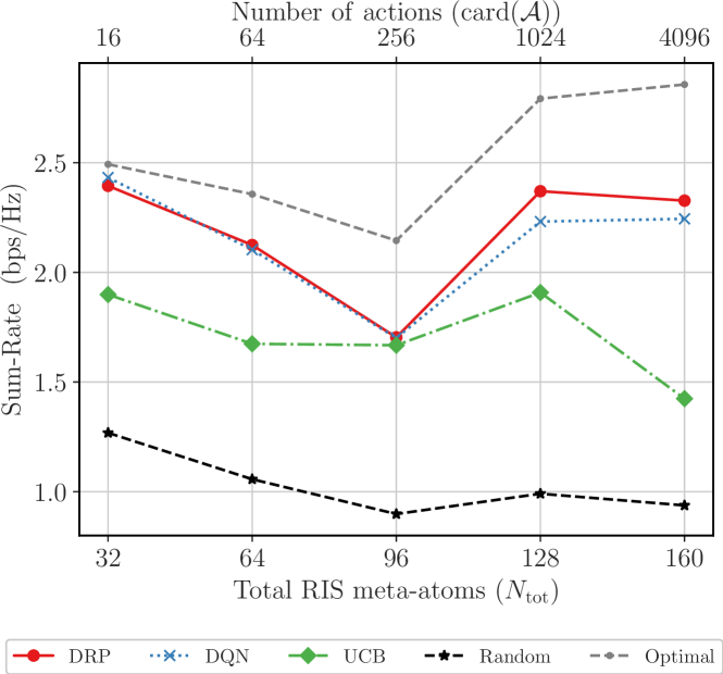
Figure 3: Sum-rate performance of the compared algorithms as the number of RIS elements and the dimension of the action space increase. The BS transmit power $P$ was set to $40~{}{\rm dBm}$.

Interestingly enough, the naive bandit approach, UCB, is also capable of sufficiently outperforming the random selection strategy, while it achieves comparable results to the DRL methods for the case of $96$ RIS elements. At the same time, Fig. 3 shows that its performance degrades at the largest trial and we expect the trend to continue in increasing RIS sizes. Nevertheless, it can be inferred that the formulation of the sum-rate maximization problem as a MAB approach allows for channel-agnostic strategies to be deployed, albeit with relatively limited capabilities.

In Fig. 4, the attained rewards during the training process of the DRL algorithms are depicted, for the setup with $128$ total RIS elements. For clarity, only the first $15000$ iterations are shown (approximately $30\%$ of the training period), in which variations during training are prominent. It can be observed that the learning curve of the DQN is steeper than that of DRP, although they both reach their common peak plateau at approximately the same time. Let it be noted that for this part of the evaluation, the actions are selected with the exploration policy (i.e. the $\epsilon$-greedy selection), which results in lower reward values, compared with the final evaluation of the learned (deterministic) policies.

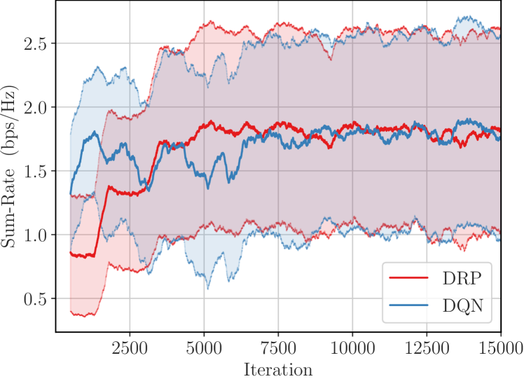
Figure 4: Training curves of the compared DRL algorithms for the first portion of the training period. The curves are smoothed by averaging within a rolling window of $300$ iterations, and the shaded areas represent the accompanying standard deviations. $P$ is set to $40~{}{\rm dBm}$ and $N_{\rm tot}$ to $96$.

To investigate the effect of the transmit power $P$ on the performance of the DRL algorithms, we repeat the evaluation process for the trial with $96$ total RIS elements, while varying $P$. The normalized average sum rates, with respect to the optimal rate given by exhaustive search, are given in Table III. The employed algorithms are mostly unaffected by the changes in $P$, performing in a similar manner (with respect to the optimal policy of exhaustive search), in all regimes.

TABLE III: Normalized Average Sum Rates for Varying Power.

$P~{}{\rm(dBm)}$	10	20	30	40	50
DRP	0.728	0.791	0.787	0.800	0.746
DQN	0.731	0.754	0.775	0.809	0.737

VI Conclusion

This paper addressed the sum-rate maximization problem in RIS-empowered multi-user MISO systems using RL techniques. Motivated by the IID assumption about the channel realizations and the immediate rate feedback, we suggested a treatment of the problem under the MAB framework, instead of the traditional MDP formalism. We proposed a DRL bandit algorithm equipped with a reward prediction network to estimate average sum rates per action (RIS configuration and precoder selection) and the $\epsilon$-greedy exploration behavior. The numerical evaluation process in a multi-RIS system established that the method compares equally with the state-of-the-art DQN algorithm, while being simpler in terms of interpretability, number of hyper-parameters, and neural network requirements. Finally, we demonstrated that our MAB-based UCB approach attains competitive performance in certain cases without the need for any channel observation.

References

- [1] W. Saad et al., “A vision of 6G wireless systems: Applications, trends, technologies, and open research problems,” IEEE Network, vol. 34, no. 3, pp. 134–142, Jun. 2020.
- [2] M. Di Renzo et al., “Smart radio environments empowered by reconfigurable AI meta-surfaces: An idea whose time has come,” EURASIP J. Wireless Commun. Netw., vol. 2019, no. 1, pp. 1–20, May 2019.
- [3] S. Lin et al., “Adaptive transmission for reconfigurable intelligent surface-assisted OFDM wireless communications,” IEEE J. Sel. Areas Commun., vol. 38, no. 11, pp. 2653–2665, Nov. 2020.
- [4] G. C. Alexandropoulos et al., “Reconfigurable intelligent surfaces for rich scattering wireless communications: Recent experiments, challenges, and opportunities,” IEEE Commun. Mag., vol. 59, no. 6, pp. 28–34, Jun. 2021.
- [5] E. Calvanese Strinati et al., “Wireless environment as a service enabled by reconfigurable intelligent surfaces: The RISE-6G perspective,” in Proc. Joint EuCNC & 6G Summit, Porto, Portugal, Jun. 2021.
- [6] C. Huang et al., “Reconfigurable intelligent surfaces for energy efficiency in wireless communication,” IEEE Trans. Wireless Commun., vol. 18, no. 8, pp. 4157–4170, Aug. 2019.
- [7] “AI and ML – Enablers for beyond 5G networks,” White Paper, 5G PPP Technology Board, May 2021.
- [8] S. Zhang et al., “AIRIS: Artificial intelligence enhanced signal processing in reconfigurable intelligent surface communications,” China Commun., vol. 18, no. 7, pp. 158–171, 2021.
- [9] C. Huang et al., “Indoor signal focusing with deep learning designed reconfigurable intelligent surfaces,” in Proc. IEEE SPAWC, Cannes, France, Jul. 2019.
- [10] A. Taha et al., “Deep reinforcement learning for intelligent reflecting surfaces: Towards standalone operation,” in Proc. IEEE SPAWC, Atlanta, USA, May 2020.
- [11] C. Huang et al., “Reconfigurable intelligent surface assisted multiuser MISO systems exploiting deep reinforcement learning,” IEEE J. Sel. Areas Commun., vol. 38, no. 8, pp. 1839–1850, Aug. 2020.
- [12] K. Feng et al., “Deep reinforcement learning based intelligent reflecting surface optimization for MISO communication systems,” IEEE Wireless Commun. Lett., vol. 9, no. 5, pp. 745–749, May 2020.
- [13] C. Huang et al., “Multi-hop RIS-empowered terahertz communications: A DRL-based hybrid beamforming design,” IEEE J. Sel. Areas Commun., vol. 39, no. 6, pp. 1663–1677, Jun. 2021.
- [14] J. Kim et al., “Multi-IRS-assisted multi-cell uplink MIMO communications under imperfect CSI: A deep reinforcement learning approach,” 2021, [Online] https://arxiv.org/pdf/2011.01141.pdf.
- [15] X. Liu et al., “RIS enhanced massive non-orthogonal multiple access networks: Deployment and passive beamforming design,” IEEE J. Sel. Areas Commun., vol. 39, no. 4, pp. 1057–1071, Apr. 2021.
- [16] M. Samir et al., “Optimizing age of information through aerial reconfigurable intelligent surfaces: A deep reinforcement learning approach,” IEEE Trans. Veh. Technol., vol. 70, no. 4, pp. 3978–3983, Apr. 2021.
- [17] H. Yang et al., “Deep reinforcement learning-based intelligent reflecting surface for secure wireless communications,” IEEE Trans. Wireless Commun., vol. 20, no. 1, pp. 375–388, Jan. 2021.
- [18] G. Lee et al., “Deep reinforcement learning for energy-efficient networking with reconfigurable intelligent surfaces,” in Proc. IEEE ICC, Dublin, Ireland, Jun. 2020.
- [19] X. Gao et al., “Machine learning empowered resource allocation in IRS aided MISO-NOMA networks,” 2021, [Online] https://arxiv.org/pdf/2103.11791.pdf.
- [20] A. Al-Hilo et al., “Reconfigurable intelligent surface enabled vehicular communication: Joint user scheduling and passive beamforming,” 2021, [Online] https://arxiv.org/pdf/2101.12247.pdf.
- [21] A. Alkhateeb et al., “Channel estimation and hybrid precoding for millimeter wave cellular systems,” IEEE J. Sel. Topics Signal Process., vol. 8, no. 5, pp. 831–846, Oct. 2014.
- [22] S. Lin et al., “Reconfigurable intelligent surfaces with reflection pattern modulation: Beamforming design, channel estimation, and achievable rate analysis,” IEEE Trans. Wireless Commun., vol. 20, no. 2, pp. 741–754, Feb. 2021.
- [23] I. Alamzadeh et al., “A reconfigurable intelligent surface with integrated sensing capability,” Scientific Reports, vol. 11, no. 1, p. 20737, 2021.
- [24] V. Mnih et al., “Human-level control through deep reinforcement learning,” Nature, vol. 518, no. 7540, pp. 529–533, 2015.
- [25] R. Agrawal, “Sample mean based index policies with regret for the multi-armed bandit problem,” Adv. Applied Probability, vol. 27, no. 4, pp. 1054–1078, 1995.