Why pseudo-complex General Relativity? and Applications

Abstract

A brief discussion on the pseudo-complex General Relativity is presented. It is shown that this theory is a viable extension of GR, with deviations centered near to the event horizon. The theory introduces a dark energy accumulation, due to the coupling to the central mass. Predictions of this theory are resumed, as for example the structure in an accretion disk, with a dark ring followed by a bright ring further in. The current Event Horizon Telescope observation of M87 is not able to discriminate between GR and pcGR, due to a low resolution. Further predictions are also discussed, as the physics of neutron stars, the redshift at the surface of the star and Quasi Periodic Object.

1 Introduction

General Relativity (GR) is one of the best tested theories in existence. Solar system experiments [1] confirm the theory, as recent observations of gravitational waves [2] and the observation of a black hole shadow by the Event Horizon Telescope (EHT) [3].

Nevertheless, one has to keep testing a theory at its extreme limits, as for very strong gravitational fields. Though, the EHT observation is consistent with GR, its resolution is not sufficient to discriminate theories which only deviate from GR near the event horizon. Further, there are conceptual problems in the case of a black hole, as the singularity in its center, the information loss and the existence of an event horizon which separates the inner region from the outer one. The existence of an event horizon is a matter of opinion. The event horizon is just a coordinate singularity and there exist others, well established ones. However, this one is the result of a strong gravitational fields and it may bother that the interior of a black hole ”in the corner of a room” cannot be accessed.

One proposal to extend GR is the pseudo-complex General Relativity (pcGR) which makes definite predictions for the region near the event horizon [4, 5, 6, 7] and also avoids the event horizon. The theory has no singularity and information can get out of the black hole, because of that rather called a black star, though, in many respects this dark star behaves like a black hole. Deviations from GR are only noticeable near the event horizon. Less massive object, as neutron stars, behave in pcGR as they do in GR.

In this contribution, I present the motivation for the pcGR and why it is a viable proposal for an extension of GR. Also, some of the predictions made by this theory will be resumed.

2 An algebraic extension of General Relativity

Earlier attempts on extending GR algebraically have been proposed by A. Einstein [8, 9] and M. Born [10, 11]. Einstein extended the metric to a complex one, where the real part is the metric used in GR and the imaginary component is associated to the electromagnetic energy-momentum tensor. The motivation was to unify GR with Electrodynamics, but unfortunately in the limit of small curvature the theory of Electrodynamics was not recovered and this approach was abandoned. This extension is equivalent to introducing complex coordinates instead of $x^{\mu}$ [7]. M. Born’s motivation was different: He noted that coordinates and momenta are not treated equivalently, as is done in Quantum Mechanics. He introduced the concept of complementary and added a metric term quadratic in the momenta. In order to observe units, the momentum term carries a dependence on a minimal length scale factor. This renders integrals over momenta finite, another reason why M. Born advocated this extension. The appearance of a minimal length scale, as a parameter, has also the advantage that Lorentz symmetry is not broken. Later, E.R. Caianiello [12] modified M. Born’s length element and the effects of the minimal length were discussed in [13].

All these extensions can be summarized under algebraic extensions. In an algebraic extension the coordinates are redefined as

$$x^{\mu} \rightarrow X^{\mu}~{}=~{}x^{\mu}+\sum_{k}a_{k}y^{\mu}_{k}$$

$$a_{k}a_{p} = \sum_{q}C_{kpq}a_{q}~{}~{}~{}.$$ (1)

The algebraic relation in the second line in (1) is the reason to call it an algebraic extension. The meaning of $y^{\mu}_{k}$ has to be deduced for each type of extension.

The simplest example is the complex extension $X^{\mu}=x^{\mu}+iy^{\mu}$, with $i^{2}=-1$, as proposed in [14]. Another, not so well known extension, is to pseudo-complex coordinates (pc) (also called hyperbolic coordinates) $X^{\mu}=x^{\mu}+Iy^{\mu}$, with $I^{2}=+1$.

There are many more possible coordinate systems, but the important point is that in [15] all possible algebraic extensions were investigated if they contain ghost and/or tachyon solutions, considered as rendering a theory inconsistent. They found that only two algebraic versions of the coordinates are allowed, namely real coordinates, leading to GR, and pseudo-complex coordinates, leading to a theory called the pseudo-complex General Relativity. The main path in [15] is to consider the weak field limit and determine the propagators of gravitational waves. In this approach and restricting here to the complex or pseudo-complex extension only, two types of propagators appear, one with a factor of 1 and another with $i^{2}$ or $I^{2}$, for the complex and pseudo-complex case respectively. In the complex case $i^{2}=-1$ and refers thus to a ghost solution. Only in the pseudo-complex case the factor $I^{2}$ is still 1, rendering this extension as the only viable one.

For this reason, the pcGR was considered as a viable extension to GR. In pcGR the infinitesimal length square element has the same form as in GR, but now in terms of the pc-variables:

$$d\omega^{2} = g_{\mu\nu}(X)dX^{\mu}dX^{\nu}$$

$$g_{\mu\nu} = g^{R}_{\mu\nu}+Ig^{I}_{\mu\nu}~{},~{}X^{\mu}~{}=~{}x^{\mu}+Iy^{\mu}~{}~{}~{}.$$ (2)

with, this the length element acquires the form

$$d\omega^{2} = \left\{g^{R}_{\mu\nu}\left[dx^{\mu}dx^{\nu}+dy^{\mu}dy^{\nu}\right]+g^{I}_{\mu\nu}\left[dx^{\mu}dy^{\nu}+dy^{\mu}dx^{\nu}\right]\right\}$$ (3)

$$+I\left\{g^{I}_{\mu\nu}\left[dx^{\mu}dx^{\nu}+dy^{\mu}dy^{\nu}\right]+g^{R}_{\mu\nu}\left[dx^{\mu}dy^{\nu}+dy^{\mu}dx^{\nu}\right]\right\}~{}~{}~{}.$$

Concerning the real part, all formerly mentioned extensions, mentioned above, can be accommodated, i.e., it also contains a minimal length. Because a particle can move only along a real path, the pseudo-imaginary component of the length element has to vanish, which leads to the constraint

$$g^{I}_{\mu\nu}\left[dx^{\mu}dx^{\nu}+dy^{\mu}dy^{\nu}\right]+g^{R}_{\mu\nu}\left[dx^{\mu}dy^{\nu}+dy^{\mu}dx^{\nu}\right] = 0~{}~{}~{}.$$ (4)

To solve (4) is particular easy in a flat space, with $g^{R}_{\mu\nu}=\eta_{\mu\nu}$ and $g^{I}_{\mu\nu}=0$. The constraint then reduces to (skipping a factor of 2)

$$\eta_{\mu\nu}dx^{\mu}dy^{\mu} = 0~{}~{}~{},$$ (5)

which is nothing but the standard dispersion relation with the solution $y^{\mu}$ $\sim$ $u^{\mu}$, i.e., $y^{\mu}$ is proportional to the 4-velocity. For dimensional reasons, a minimal length scale factor has to be introduced, and using $c=1$ the $y^{\mu}$ acquires the form

$$y^{\mu} = lu^{\mu}~{}~{}~{}.$$ (6)

Thus, the $y^{\mu}$ components are related to the minimal length scale. In this case the length element of E.R. Caianiello can be recovered. A more general, approximate solution of (4) is given in [7].

In order to obtain the extended Einstein equations, one uses the standard form of the action

$$S=\int dX^{4}\sqrt{-g}\left({\cal R}+2\alpha\right)~{}~{}~{},$$ (7)

where ${\cal R}$ is the pc-Riemann scalar and $\alpha$ is related to the dark, energy as in GR. For cosmological models, the $\alpha$ has to be a constant due to translational invariance. However, in a central problem the $\alpha$ may depend on $r$ and with rotation included also on the azimuthal angle $\theta$. In contrast to GR, all elements in (7) are pseudo-complex. For a mathematical introduction on the analysis of pc-variables and for further references, please consult [5].

The action principle $\delta S$ = 0 is applied. In former publication a modified variational principle was proposed. But as shown already on the last pages of [5], including the constraint (4) it is equivalent to use the standard variational principle. Neglecting the minimal length finally leads to the Einstein equations

$${\cal R}_{\mu\nu}-\frac{1}{2}g_{\mu\nu}{\cal R} = 8\pi T_{\mu\nu}^{\Lambda}~{}~{}~{}.$$ (8)

For more details, please consult [7]. In a current investigation [16], the influence of a minimal length within pcGR is investigated, with the result that only for masses of the order of $l$ appreciable changes occur, thus justifying to neglect $l$ for macroscopic black holes. The energy-momentum tensor depends on a couple of parameters which leaves space for further assumptions. This leads to the introduction of dark energy, with the density $\varrho_{\Lambda}$.

In addition to the pseudo-complex structure, pcGR assumes that dark energy accumulates near a black hole (or a mass in general), but only noticeable near the event horizon. This is a result of semi-classical calculations in Quantum Mechanics [17, 18], i.e., dark energy is created in a curved space-time back ground. The pcGR assumes therefore that there is a coupling between the central mass and the amount of dark energy. The ansatz for the dark energy is

$$\varrho_{\Lambda} \sim \frac{B_{n}}{r^{n+2}}~{}~{}~{},$$ (9)

with $B_{n}$ and $n$ being parameters of the theory.

This assumption implies an important principle, namely that a central mass not only curves space.time but also changes the vacuum properties of space-time near it. This coupling to the dark energy is a consequence of quantum effects and the study of pcGR therefore can help in understanding what these quantum effects might be. The other parameter is $n$, describing the fall-off of the dark energy as a function in $r$. In [4] $n=2$ was assumed, but this already violates observations in the solar system. From that, calculations were performed with $n=3$ [5], however, in [19, 20] the inspiral wave of a gravitational wave was fitted to pcGR and concluded that $n$ has to be larger than 3. From then on, the value $n=4$ is assumed, which is also in better accordance to the $r$-dependence obtained in [18]. Nevertheless, one has to keep in mind that $B_{n}$ and $n$ are parameters, converting pcGR to a phenomenological theory. There exist studied for the accumulation of dark matter in a black hole. dark matter does not interact strongly with matter, only through gravitation. In contrast, dark energy does interact with matter [18] and should play a more dominant role.

The metric in pcGR, including rotation, has the form [7] (there is an error in the $g_{11}$-component, corrected here)

$$g_{00} = -\frac{r^{2}-2m_{0}r+a^{2}\cos^{2}\vartheta+\frac{B_{n}}{(n-1)(n-2)r^{n-2}}}{r^{2}+a^{2}\cos^{2}\vartheta}~{}~{}~{},$$

$$g_{11} = \frac{r^{2}+a^{2}\cos^{2}\vartheta}{r^{2}-2m_{0}r+a^{2}+\frac{B_{n}}{(n-1)(n-2)r^{n-2}}}~{}~{}~{},$$

$$g_{22} = r^{2}+a^{2}\cos^{2}\vartheta~{}~{}~{},$$

$$g_{33} = (r^{2}+a^{2})\sin^{2}\vartheta+\frac{a^{2}\sin^{4}\vartheta\left(2m_{0}r-\frac{B_{n}}{(n-1)(n-2)r^{n-2}}\right)}{r^{2}+a^{2}\cos^{2}\vartheta}~{}~{}~{},$$

$$g_{03} = \frac{-a\sin^{2}\vartheta~{}2m_{0}r+a\frac{B_{n}}{(n-1)(n-2)r^{n-2}}\sin^{2}\vartheta}{r^{2}+a^{2}\cos^{2}\vartheta}~{}~{}~{}.$$ (10)

It is illustrative to calculate the energy-momentum tensor within the pc-Schwarzschild limit (non-rotating star). Substituting the metric (10) into the left hand side of the Einstein equations results in the $T_{\mu\nu}$ on the right hand side of these equations. Further, for the energy-momentum tensor we define the dimensionless quantities $y=\frac{r}{m_{0}}$ and $b=\frac{B}{m_{0}^{4}}$, with which this tensor acquires the form (the signature of the metric is (-+++))

$$8\pi\left(T^{\mu}_{~{}\nu}\right) = \left(\begin{array}[]{cccc}-\frac{b}{2y^{6}}&0&0&0\\ 0&-\frac{b}{2y^{6}}&0&0\\ 0&0&\frac{b}{y^{6}}&0\\ 0&0&0&\frac{b}{y^{6}}\\ \end{array}\right)~{}=~{}8\pi\left(\begin{array}[]{cccc}-\varrho^{\Lambda}&0&0&0\\ 0&p^{\Lambda}_{r}&0&0\\ 0&0&p^{\Lambda}_{\vartheta}&0\\ 0&0&0&p^{\Lambda}_{\vartheta}\\ \end{array}\right)~{}~{}~{}.$$ (19)

From (19) the Riemann scalar $R=-\frac{b}{y^{6}}$ is deduced. It is clearly seen that the energy-momentum tensor describes an anisotropic fluid with a different pressure in the radial compared to the angular directions.

From these consideration, it should be clear that the pseudo-complex extension of GR has to be considered seriously. The next question is: What kind of prediction the pcGR is making and in what they differ to GR?

3 Resumé of some predictions of pcGR

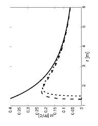
Figure 1: The orbital frequency of a point particle in a circular orbit as a function in $r$. The rotational parameter is $a=0.95m_{0}$. The upper curve is the result as obtained in GR while the two lower curves are from pc-GR, for $n=3$ (left curve) and $n=4$ (right curve).

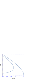
Figure 2: Limits for stable orbits ($n=4$) as a function in the rotational parameter $a$. The upper curve is the result of GR, which marks the position of the Innermost Stable Circular Orbit (ISCO). In pc-GR there are no stable orbits to the left of the lower curve.

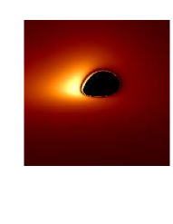
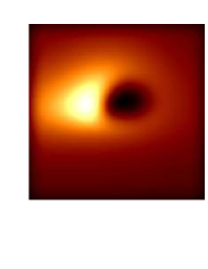
Figure 3: Simulations of the accretion disc in M87, using the model of Ref. [21] and $a=0.95m_{0}$. The left panel is for a resolution of 5$\mu$as. The right panel is for 20$\mu$ as, a little bit less than 24$\mu$as, the resolution reported by the EHT. The inclination angle of the disc with respect to the observer is 70^o.

3.1 Structure of accretion disks

In [5, 6, 22, 23] simulations of a thin, optical thick accretion disk [21] where published and compared to GR.

In order to understand the results of the simulations, we have to explain how the orbital frequency of a particle in a circular orbit changes with respect to the radial distance and where do stable orbits exist: In Fig. 1 this orbital frequency is depicted for the Kerr parameter $a=0.95m_{0}$. Clearly seen is the appearance of a maximum, at which two neighboring orbitals have the same orbital frequency, which results in less friction and less emission if light, marking the position of the dark ring. In Fig. 2 the range of stable orbits is depicted [24]. The upper line corresponds to GR, where for $a=0$ the last stable orbit is at $6m_{0}$ and it approaches $1m_{0}$ for $a=1m_{0}$. The lower curve encircles the area where no stable orbit exists in pcGR. Note that above $a=0.5m_{0}$ all orbits are stable in pcGR and they can reach the point where the orbital frequency has a maximum. Below $a=0.5m_{0}$ the pcGR follows the GR 1, i.e., similar results are expected, though, the last stable orbit is further in in more light is emitted.

In Fig. 3, on the left panel the simulation for a high resolution is given. It is clearly observed that the disk has a dark ring, followed further in by a bright one. The dark ring is the consequence of the maximum in the orbital frequency as a function on the radial distance. The right panel in Fig. 3 shows the same but with a low resolution of 20$\mu$as, a bit lower than the EHT. One can see that the ring structure is washed out. Thus, in order to see the ring structure one has to increase the resolution of the EHT significantly. It also means that the observations are consistent with GR and pcGR. Thus, this particular prediction of pcGR cannot be verified yet and one has to await a much better resolution.

3.2 Redshift

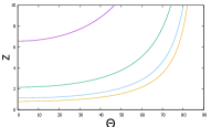
Figure 4: Redshift $z$ at $r=\frac{3}{2}m_{0}$ for different rotation parameter values $a$, as a function on the azimuth angle $\theta$. From the upper to the subsequent lower curves the $a$-value varies from 0.2$m_{0}$, 0.5$m_{0}$, 0.8$m_{0}$ to 1.0$m_{0}$.

There is hopefully a possibility to see some difference between GR and pcGR, but it depends on the non-existence of a jet. Because the jet is a consequence of the presence of an accretion disk, this is equivalent to demand that there is no accretion disk.

The only observable black hole up to now by the EHT, which may have no accretion disk, is SgrA* in the center of our Galaxy. Observational results are still pending.

In Fig. 4 the redshift at the surface of the black star is plotted as a function on the azimuthal angle $\theta$. The different curves correspond to different $a$-values. The redshift is lowered toward the poles and if $a$ is very large (above 0.5$m_{0}$), the redhift has values of 1-2. In other words, infalling matter, which collides with the surface, should emit light and its reshifted frequency has to be detected by an observer on earth. Toward the orbital plane the redshift is too large and no hope exist to detect it. I.e., there is only hope to see something near the poles, which requires that, first, the matter has to fall onto the surface near the poles and, secondly, there is no jet present (due to an accretion disk), which would over-shine the effect.

3.3 Neutron Stars

In the first decade of this century a neutron star with 2.05 solar masses was observed [25], while until then one did not expect masses larger than 2, with a ”realistic” equations of state. In [26] a theory for neutron stars was developed which finally could accommodate the mass. Recently, in observing gravitational waves [27], a further candidate with 2.5 solar masses was suggested. Since then, many contributions can be found which can explain these masses. The central point is how to change the equation of state of the matter in order to support a greater mass. This seems a bit unsatisfactory, because greater masses can obviously obtained by changing appropriately the equation of state, such that larger masses can be obtained.

Figure 5: Mass vs the radius of a black star. A linear relation between the dark energy density and mass density in the interior of the star was assumed.

In pcGR this is not a problem: The accumulation of dark energy, due to the coupling of the mass to it, accommodates well larger masses, as is shown in [5, 28]. There, the coupling of the mass density with the dark energy density was assumed to be linear

$$\varrho_{\Lambda} = \alpha\varrho_{\rm m}~{}~{}~{}.$$ (20)

The index ${\rm m}$ refers to the mass density and the index $\Lambda$ to the dark energy density. Also here the mass couples to the dark energy. In fig. 5 several curves for different $\alpha$-values are depicted. Stars up to 6 solar masses were found stable. However, if these dark stars can still be considered neutron stars is questionable. In our view, there is a continuous shift from a classical neutron star, with a particle beam, to a classical black hole, where the emitted light of a beam shifts to a large redshift or disappears due to unknown processes.

In [29] semi-classical calculations [17] were performed which resulted in a more complicated relation for the coupling of the matter density to the dark energy density. As a result, the coupling diminished toward to the surface of the black star and much higher masses were obtained.

All calculations relied on the hadronic model for the matter, published in [26]. With increasing density this model reaches its limit and due to lack of confidence no further calculations can be done. In this respect, new models for the matter at high density are required.

Therefore, we predict the existence of stellar objects which behave as a neutron star, emitting a beam whose emitted light has a large redshift, and also have too large masses to be explained by standard models.

3.4 Quasi Periodic Objects (QPO)

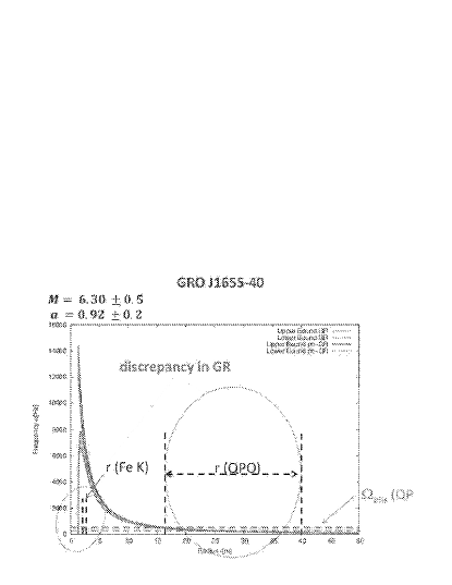
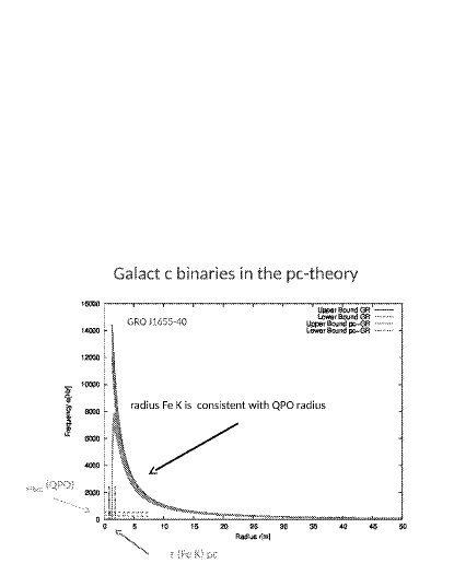
Figure 6: The orbital frequency of a particle in a circular orbit versus the radial distance. The upper curve is for GR while the lower one for pcGR and $n=3$ (for $n=4$ the result is not much different). The width of a line is a measure of the error in the $a$-parameter. The horizontal dashed line is from fitting to the orbital frequency observed, with its experimental error. The vertical dashed line is for adjusting to the redshift of the emitted line.

QPO’s are assumed to be excitations within an accretion disks (hot spots) which are circling around with the disk, They are observed in accretion disks of galactic black holes and also in the disks of stellar black holes [30, 31, 32, 33]. Knowing the frequency and the formula for the orbital frequency in a circular orbit, a distance value can be deduced. If this is the real distance has to be verified by another measurement, as the redshift of the line emitted. Unfortunately, for galactic black holes this has not been seen yet. Because galactic black holes are fairly well isolated (no large partner nearby), the interpretation of the QPO as a co-rotating hot spot in the accretion disk is quite well established. For stellar black holes one also observes QPO’s and simultaneously the rotation frequency and the redshift of the emitted line. Therefore, from the redshift one can deduce also a distance. From both observations the same distance has to result, for consistency. In Fig. 6 the orbital frequency of a particle in a circular orbit is depicted. The upper line refers to GR while the lower line to pcGR. The horizontal dashed line is from adjusting to the observed orbital frequency and the vertical line from the observed redshift of the emitted line.

The problem is now, using the formulas from GR both distances are not the same, but they are the same in pcGR. One might say that this proves pcGR, however, one has to take into account possible effects of the stellar partner onto the accretion disk around the black hole. It was shown that one can indeed explain the discrepancy in GR by this influence of the stellar partner, using models [34]. Though pcGR is easier to apply here, not involving further assumptions, the fact that one can reconcile the measurement with GR makes it inconclusive.

Conclusions

I have presented the motivation for the algebraic extension of GR to pseudo-complex coordinates. The pcGR turns out to be the only viable algebraic extension.

The structure of pcGR was explained and its differences to GR pointed out.

A theory has to be verifiable, which is exactly the case for pcGR. Several predictions were presented:

• The appearance of a dark ring followed further in by a bright ring, which is due to the dependence of the orbital frequency of a particle in a circular orbit. Unfortunately, the resolution of the EHT is not sufficient to distinguish pcGR from GR, until a much better resolution is reached.

• The redshift of light emitted from the surface of the dark star, as a function of the azimuthal angle was determined. We predict that matter falling onto the surface near the poles can emit light with a redshift between 1-2, which should be observable. However, this is linked to the condition that the massive object is not accompanied by an accretion disk, which would include a jet near the poles. This jet would over-shine the effect described. The black hole in the center of our galaxy, SgrA*, is thought not to have an accretion disk, so there is some hope.

• The theory allows a stable star for any mass value, i.e., it easily accommodates larger masses for neutron stars, without any further assumptions, using an equation of state known. Possibly, there is a smooth transition from stellar object which behave as a neutron star with a beam, to stellar objects where the beamdisappears. The uncertainty here is the structure (equation of state) within the star.

• Quasi Periodic Objects, which are observed in galactic centers and in binary systems with one black hole. Here, the simultaneous measurement of the orbital frequency and the redshift of the emitted line lead to the same distance, contrary to GR. However, investigating the effect of the stellar visible partner on the structure of the accretion disk, using models, can still accommodate GR. This is a case where pcGR leads to a simple explanation, but still the situation is not settled yet.

As can be seen, the pcGR is a realistic extension of GR, but further observations with their improvements have to be made.

References

References

- [1] C. M. Will, Living Rev. Relativ. 9 (2006), 3.
- [2] Abbott B. P. et al. (LIGO Scientific Collaboration and The Virgo Collaboration), 2016c, Phys. Rev. Lett. 116, 241103.
- [3] The Event Horizon Telescope collaboration, ApJ 875 (2019), L1.
- [4] P. O.Hess and W. Greiner, Int. J. Mod. Phys. E 18, 51 (2009).
- [5] Hess P. O., Schäfer M. and Greiner W., Pseudo-Complex General Relativity; Springer: Heidelberg, Germany, 2015.
- [6] P. O. Hess and E. López-Moreno, Universe 5 (2019), 191.
- [7] P. O. Hess, Progr. Part. Nucl. Phys. 114 (2020), 103809.
- [8] A. Einstein, Ann. Math. 46, 578 (1945).
- [9] A. Einstein, Rev. Mod. Phys. 20. 35 (1948).
- [10] M. Born, Proc. Roy. Soc. A 165, 291 (1938).
- [11] M. Born, Rev. Mod. Phys. 21, 463 (1949).
- [12] E. R. Caianiello, Nuovo Cim. Lett. 32 (1981), 65.
- [13] A. Feoli G. Lambiase, G. Papini and G. Scarpetta, Phys. Lett. A 263 (1999), 147.
- [14] C. L. M. Mantz and T. Prokopex, arXiv:gr-qc.0804.0213
- [15] P. F. Kelly and R. B. Mann, Class. and Quant. Grav. 3, 705 (1986).
- [16] L. Maghlaoui and P. O. Hess, manuscript in preparation (2022).
- [17] N. D. Birrell and P. C. W. Davies, Quantum Fields in Curved Space (Cambridge University Press, The Edinbugh Building, Cambridge, 1994).
- [18] M. Visser, Phys. Rev. D 54 (1996) 5116.
- [19] A. Nielsen and O. Birnholz, Astron. Nachr. 339 (2018), 298.
- [20] A. Nielsen and O. Birnholz, Astron. Nachr. 340 (2019), 116.
- [21] D. N. Page and K. S. Thorne, Astrophys. J. 191 (1974), 499.
- [22] T. Boller, P. O. Hess, A. Müller ands H. Stöcker, MNRAS:Letters 485 (2019), L34.
- [23] P. O. Hess, T. Boller, A. Müller and H. Stöcker, MNRAS:Letters 485 (2019), L121.
- [24] T. Schönenbach, G. Caspar, P. O. Hess, T. Boller, A. Müller and W. Greiner, Mon. Not. R. Astron. Soc. 442 (2014),121–130.
- [25] D. J. Nice, E. M. Splaver, I. H. Stairs, O. Loehmer, A. Jessner, M. Kramer and J. M. Cordes, ApJ 634 (2005), 1242.
- [26] V. Dexheimer and S. Schramm, The Astrophys. J. 683 (2008) 943.
- [27] R. Abbott, T. D. Abbott, F. Acernese, et al., arXiv:2111.03606[gr-qc]; Report No.: LIGO-P200031
- [28] I. Rodríguez, P. O. Hess, S. Schramm and W. Greiner, J. Phys. G 41, (2014), 105201.
- [29] G. Caspar, I. Rodríguez, P. O. Hess and W. Greiner, Int. J. Mod. Phys. E 25 (2016), 1650027.
- [30] T. H. Belloni, A. Sanna and M. Mendz, MNRAS 426 (2012), 1701.
- [31] R. T. Hynes, D. Steeghs, J. Casares, P. A. Charles and K. O’Brian, The Astrophys. J. 609 (2004), 317.
- [32] R. C. Reis, A. Fabian, R. R. Ross, G. Miniutti, J. M. Miller and C. Reynolds, MNRAS 387 (2008), 1489.
- [33] J. Steiner, J. McClintock, G. Jeffrey et al., 38th COSPAR Scientific Assembly, 18–15 July, Bremen, Germany, 2010).
- [34] D. Lai, W. Fu, D. Tsang, J. Horak and C. Ya, Proc. of the Intern. Astron. Union 290 (2012), 57.